Gilbert’s disc model conditioned on the square lattice
July 15, 2026
Abstract
We present a new percolation model on the two-dimensional lattice, which can be seen as a conditioned version of continuous percolation on the plane. Let us place a point uniformly at random in each cell of the grid \(\mathbb{Z}^2\). These points correspond to the vertices of our graph, and we connect two points by an edge if their distance is less than a fixed radius \(R\). We are interested in the radius from which there exists almost surely an infinite connected component. We also study two other critical radii specific to the geometry of our model: the smallest radius such that there exists a positioning of the points for which there is an infinite connected component, and the radius from which all points are connected to each other.
1 Introduction↩︎
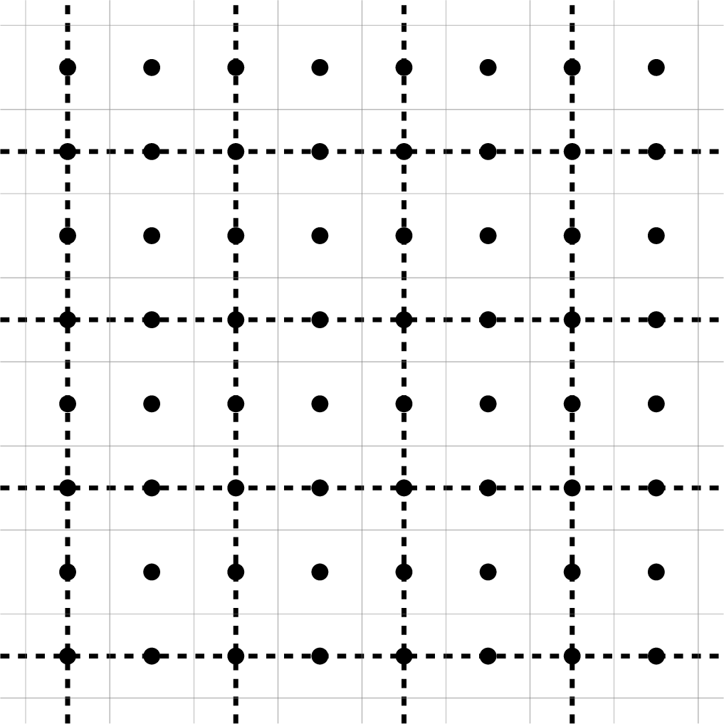
Let \(R\in \mathbb{R}_+\) be a fixed radius, and let \(d:\mathbb{R}^2\times\mathbb{R}^2\to\mathbb{R}_+\) be a distance on \(\mathbb{R}^2\). In the following of the article, we mainly focus on \(\mathcal{L}_p\) distance. We consider a collection \(P=(P_{i,j})_{(i,j)\in\mathbb{Z}^2} = (X_{i,j},Y_{i,j})_{(i,j)\in\mathbb{Z}^2}\) of points of \(\mathbb{R}^2\), such that for any \((i,j)\in\mathbb{Z}^2\), \(X_{i,j}\in [i,i+1]\) and \(Y_{i,j}\in [j,j+1]\). We denote the set of such collections by \(\mathcal{P}=\prod_{(i,j)\in\mathbb{Z}^2} [i,i+1]\times[j,j+1]\).
1.0.0.1 Complete neighbor model.
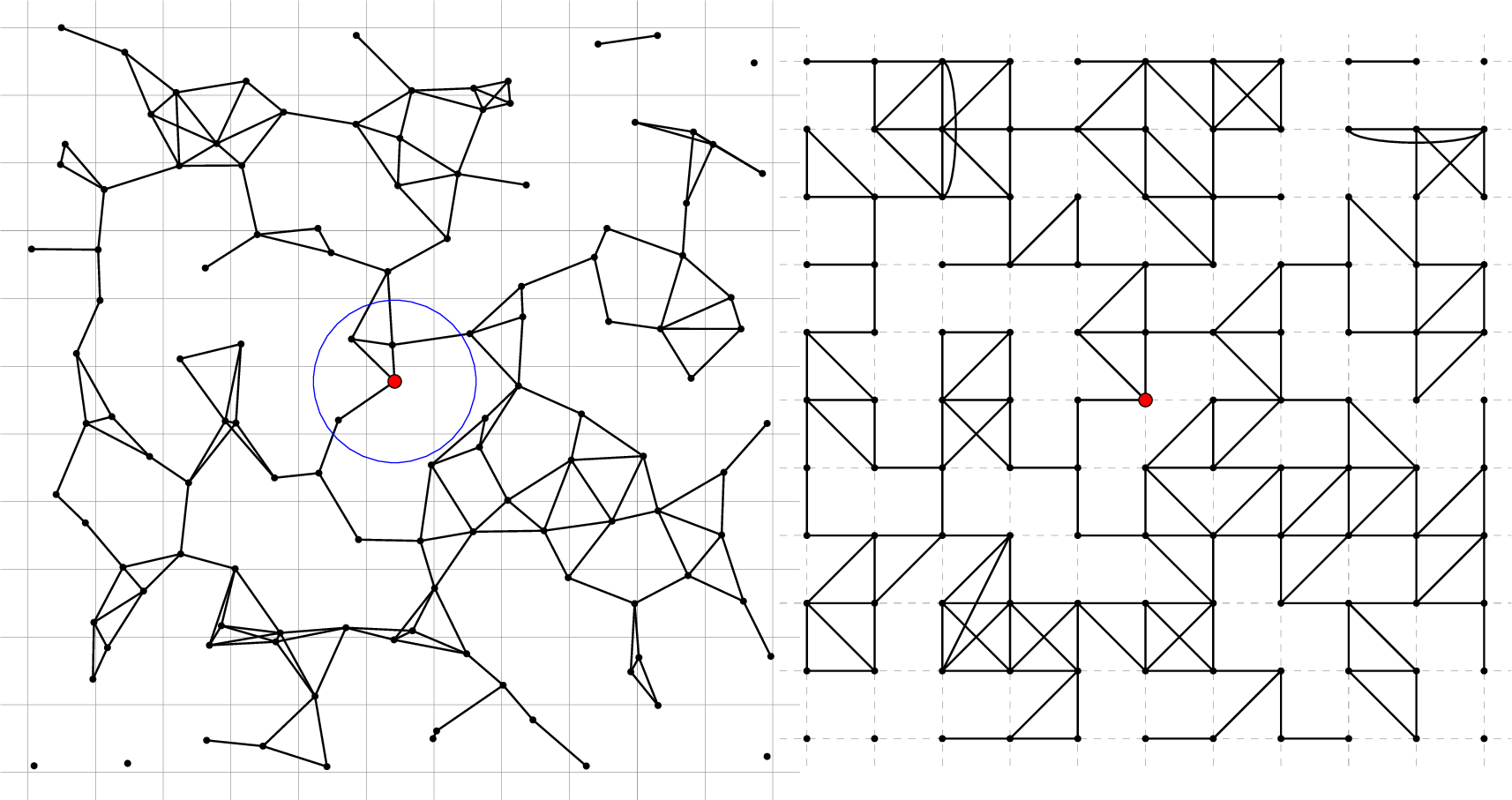
For any \(P\in\mathcal{P}\) we construct the undirected graph \(\mathcal{G}(P) = (P,E)\) where \(E = \{(P_u,P_v) : d(P_u,P_v)<R\}\), see the graph on the left of Figure 1.
We focus mainly on the projected version of \(\mathcal{G}(P)\) on the lattice \(\mathbb{Z}^2\), see the graph on the right of Figure 1, which we denote by \(\Gamma_{d,R}^{\texttt{CN}}(P)=(\mathbb{Z}^2,E_{d,R}^{\texttt{CN}}(P))\) defined by \[E_{d,R}^{\texttt{CN}}(P)=\{(u,v)\in\mathbb{Z}^2\times\mathbb{Z}^2: u \neq v \text{ and } d(P_u,P_v)\leq R\}.\] We say that such a graph \(\Gamma_{d,R}^{\texttt{CN}}(P)\) is a configuration of parameter \(R\) for the complete neighbor model. For a graph \(G=(V,E)\), we say that two vertices \(u, v\in V\) are neighbors if \((u,v)\in E\). A path between \(u\) and \(v\) is a sequence \((u_k)_{0\leq k\leq n}\) of vertices, with \(u_0=u\) and \(u_n=v\), such that \(\forall k\in\{0,...,n-1\}\), \(u_k\) and \(u_{k+1}\) are neighbors. We say that \(u\) and \(v\) are connected if there exists a path between \(u\) and \(v\). When \(V=\mathbb{Z}^2\), we denote by \(\mathcal{C}_0(G)\) the connected component of \((0,0)\), that is the set of vertices connected to \((0,0)\).
Our main focus is the typical connected components of \(\Gamma_{d,R}^{\texttt{CN}}(P)\) when the points of \(P\) are chosen independently at random, with \(P_{i,j}\) uniformly distributed in \([i,i+1]\times[j,j+1]\) for each \((i,j)\in \mathbb{Z}^2\). We denote by \(\mathbb{P}\) the corresponding point distribution on \(\mathcal{P}\), that is, the product distribution \(\mathbb{P}=\bigotimes_{(i,j)\in\mathbb{Z}^2}\mathcal{U}([i,i+1]\times [j,j+1])\), where \(\mathcal{U}(A)\) denotes the uniform distribution on \(A\). Figure 1 presents a simulation of the lattice-based Gilbert’s disc model for the Euclidean distance.
1.0.0.2 Context and connection to Gilbert’s disc model.
The complete neighbor model was first introduced in HM90?, as a new type of neighborhood for cellular automata, which allows one to observe more regular patterns than in the classical setting.
Observe that it can also be seen as a conditioned version of Gilbert’s disc model, for which points are distributed in the plane according to a Poisson process. In the most general framework of the Boolean model, also known as continuous percolation, the radii \(R\) associated with the points form a family of i.i.d. random variables Gil61?, MR96?.
On its side, the nearest neighbour model that we introduce a little later can be interpreted as a variant of independent Bernoulli percolation on the square lattice Gri99?, that presents local dependencies.
Whether for discrete or continuous percolation models, a fundamental question that has been the subject of extensive research concerns the existence or not of an infinite connected component, depending on the values of the parameters.
1.0.0.3 Percolation radii.
In our context, we define the percolation probability as the probability that the connected component \(\mathcal{C}_0(\Gamma_{d,R}^{\texttt{CN}}(P))\) is infinite, that is, \[\theta_d^{\texttt{CN}}(R) = \mathbb{P}(|\mathcal{C}_0(\Gamma_{d,R}^{\texttt{CN}}(P))|=\infty),\] and the critical radius by \[R_c^{\texttt{CN}}(d) = \sup\{R>0 : \theta_d^{\texttt{CN}}(R) = 0\}.\]
Proposition 1. Let \(d_1\) and \(d_2\) be two distances on \(\mathbb{R}^2\), and let \(R_1,R_2>0\). If for any \(z\in\mathbb{R}^2\), we have \(B_{d_1}\left(z,R_1\right)\subset B_{d_2}\left(z,R_2\right)\), then for any \(P\in\mathcal{P}\), \(E_{d_1,R_1}^{\texttt{CN}}(P)\subset E_{d_2,R_2}^{\texttt{CN}}(P)\), and as a consequence, \(\theta^{\texttt{CN}}_{d_1}(R_1)\leq\theta^{\texttt{CN}}_{d_2}(R_2).\)
The proof is straightforward. As a consequence of Proposition 1, the percolation probability \(R\mapsto\theta_d^{\texttt{CN}}(R)\) is non-decreasing. Moreover, if the model is invariant by translation (that is the case later when we consider a distance derived from a norm), there exists two distinct regimes: for \(R<R_c^{\texttt{CN}}(d)\), the graph \(\Gamma_{d,R}^{\texttt{CN}}(P)\) has almost surely no infinite connected component (sub-critical regime), while for \(R>R_c^{\texttt{CN}}(d)\), it has almost surely at least one infinite connected component (super-critical regime).
The geometry of our model also leads us to introduce two other types of critical radius, namely the total connectivity radius and the possible connectivity radius.
The total connectivity radius is the smallest radius from which all points are inside an infinite connected component. It is defined by \[R_{\max}^{\texttt{CN}}(d)=\inf\{R>0 : \forall P\in \mathcal{P}, |\mathcal{C}_0(\Gamma_{d,R}^{\texttt{CN}}(P))|=\infty\}.\] The possible connectivity radius is the smallest radius from which an infinite connected component becomes possible, in the sense that \[R_{\min}^{\texttt{CN}}(d) = \inf\{R>0 : \exists P\in\mathcal{P}, |\mathcal{C}_0(\Gamma_{d,R}^{\texttt{CN}}(P))|=\infty\}.\]
We clearly have the following inequalities \[R_{\min}^{\texttt{CN}}(d) \leq R_c^{\texttt{CN}}(d) \leq R_{\max}^{\texttt{CN}}(d).\]
1.0.0.4 Nearest neighbor model.
For a given distance \(d\), we also consider the nearest neighbor model that consists in restricting the possible connections to the four adjacent cells. Precisely, the set of edges \(E_{d,R}^{\texttt{NN}}\) of the new graph \(\Gamma_{d,R}^{\texttt{NN}}(P)\) obtained is then given by \[E_{d,R}^{\texttt{NN}}=E_{d,R}^{\texttt{CN}} \cap \{(u,v)\in\mathbb{Z}^2\times \mathbb{Z}^2 : ||u-v||_1=1\}.\]
We denote the corresponding radii with a \(\texttt{NN}\) exponent. Again, we have \[R_{\min}^{\texttt{NN}}(d) \leq R_c^{\texttt{NN}}(d) \leq R_{\max}^{\texttt{NN}}(d).\] And since \(E_{d,R}^{\texttt{NN}}\subset E_{d,R}^{\texttt{CN}}\), it follows that
\[R_{\min}^{\texttt{CN}}(d) \leq R_{\min}^{\texttt{NN}}(d)\text{, } R_{c}^{\texttt{CN}}(d) \leq R_{c}^{\texttt{NN}}(d)\text{, and } R_{\max}^{\texttt{CN}}(d) \leq R_{\max}^{\texttt{NN}}(d).\]
Proposition 2. Proposition 1 still holds for the nearest neighbor model.
1.0.0.5 \(\boldsymbol{\mathcal{L}}^p-\)norm.
Now, we consider only distances \(d\) resulting from a \(\mathcal{L}^p-\)norm on \(\mathbb{R}^2\), i.e.for any \(Q,Q' \in \mathbb{R}^2\), \(d(Q,Q')=\|Q-Q'\|_p\), where for \(Q=(x,y)\),
\[\|Q\|_p = \left \{ \begin{array}{ll} \big(|x|^p + |y|^p)^{\frac{1}{p}} & ifp\in[1,\infty);\\ \max\{|x|,|y|\} & ifp=\infty.\\ \end{array} \right.\]
From now on, when the distance considered results from the \(\mathcal{L}^p-\)norm, we put the value \(p\in[1,\infty]\) as a parameter of the graph, the set of edges and the radii instead of \(d\).
We now state the main theorems of this article, which provide exact values or boundaries of the different radii when the distance \(d\) is derived from \(\mathcal{L}^p-\)norm, for both the complete neighbor model and the nearest neighbor one.
Proposition 3. Let \(p_1,p_2\in[1,\infty]\) with \(p_1\leq p_2\). We have \[R_{\min}^{\texttt{CN}}(p_2) \leq R_{\min}^{\texttt{CN}}(p_1)\text{, } R_{c}^{\texttt{CN}}(p_2) \leq R_{c}^{\texttt{CN}}(p_1)\text{, and } R_{\max}^{\texttt{CN}}(p_2) \leq R_{\max}^{\texttt{CN}}(p_1).\] The same property holds for the nearest neighbor model.
Proof. By Proposition 1, we have for any \(P\) and \(R\), \(E_{p_1,R}^{\texttt{CN}}(P)\subset E_{p_2,R}^{\texttt{CN}}(P)\). Especially, if the connected component is infinite for the distance derived from the \(\mathcal{L}^{p_1}-\)norm, it is also infinite when the distance considered is derived from the \(\mathcal{L}^{p_2}-\)norm. This conclude the proof for the complete neighbor model. By Proposition 2, the arguments are similar for the nearest neighbor model. ◻
1.0.0.6 Main results.
For the total connectivity radius, the exact values are given in the following theorem.
Theorem 4. For \(p\in[1,\infty]\), we have \[R_{\max}^{\texttt{CN}}(p) = R_{\max}^{\texttt{NN}}(p) = \|(2,1)\|_p.\]
The proof is given in Section 2.
For the possible connectivity radius, we also give the exact values. It is totally explicit for the complete neighbor model, but "slightly less" for the nearest neighbor variation.
Theorem 5.
For \(p\in[1,\infty)\), \(R_{\min}^{\texttt{CN}}(p) = \displaystyle \min \left\{\frac{1}{2},\frac{2}{1+2^{2-\frac{1}{p}}}\right\}\) and \(R_{\min}^{\texttt{CN}}(\infty)=2/5\).
For \(p\in[1,\infty)\), we denote by \(R(p)\) the unique solution on \([0,1]\) of the equation \[\label{eqRmin4V} (2-R)^p + (3-3R)^p = (4R)^p.\qquad{(1)}\] We have \(R_{\min}^{\texttt{NN}}(p) \displaystyle = \min\left\{\frac{1}{2},R(p)\right\}\) and \(R_{\min}^{\texttt{NN}}(\infty) = 3/7\).
An important part of this article is devoted to the proof of this result, which is given in Section 3.
Finally, we improve the bounds for the critical radius.
Theorem 6. For \(p\in[1,\infty]\), we have
\(R_{\min}(p)\leq R_{c}^{\texttt{CN}}(p)\leq\displaystyle \left\|\left(1,\frac{3}{2}\right)\right\|_p\),
\(\sqrt{2-\sqrt{2}}\leq R_{c}^{\texttt{NN}}(p)\leq\displaystyle \left\|\left(1,\frac{3}{2}\right)\right\|_p\).
The proof is given in Section 4.
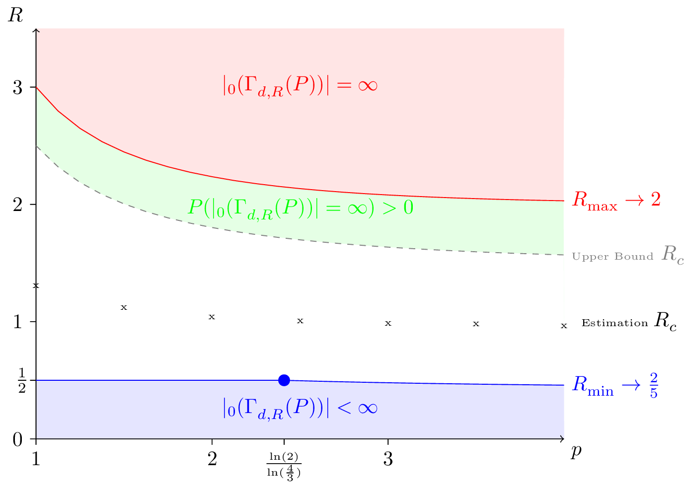
The results of those three theorems are summarized on Figure 2 for the complete neighbor model and on Figure 3 for the nearest neighbor one.

1.0.0.7 Outline of the article.
Section 2 is devoted to the proof of Theorem 4. Precisely, we show that all points are connected when \(R\geq\|(2,1)\|_p\), while if \(R<\|(2,1)\|_p\), we can construct an event of positive probability for which the origin belongs to a finite connected component. In Section 3, we prove Theorem 5, using self-avoiding paths. In order to bound \(R_{\min}^{\texttt{CN}}\) and \(R_{\min}^{\texttt{NN}}\) by above, it is sufficient to exhibit a single configuration for which there is an infinite path. For the lower bound, we provide firstly a proof quite simple for the case \(p=\infty\), then a second more general proof for any \(\mathcal{L}^p-\)norms. The strategy is to assume that there exists a configuration with an infinite self-avoiding path, and to show that a certain quantity decreases strictly along this path, which then leads to a contradiction. Section 4 is devoted to the proof of the boundaries given in Theorem 6. We define a variant of our nearest-neighbor model, and compare it with the Bernoulli percolation, with the help of a duality argument.
2 Proof of Theorem 4 (\(R_{\max}\))↩︎
Let \(p\in[1,\infty]\) be fixed. The following proof is treated for the case of the complete neighbor model. It can be adapted for the nearest neighbor model without major changes.
2.0.0.1 Upper bound.
Let \(R\geq\|(2,1)\|_p\). For any \(P_{0,0} \in [0,1]^2\) and for any \(P_{1,0} \in [1,2]\times[0,1]\), \(\|P_{1,0}-P_{0,0}\|_p\leq \|(2,1)\|_p\). It follows that the points \((0,0)\) and \((1,0)\) are neighbors in \(\Gamma_{d,R}^{\texttt{CN}}(P)\). For the same reason, the points \((-1,0)\), \((0,1)\) and \((0,-1)\) are also neighbors of \((0,0)\). By induction, all the points are connected to \((0,0)\).
2.0.0.2 Lower Bound.
Let \(\varepsilon>0\), and consider a radius \(R=\|(2,1)\|_p-\varepsilon\). We show that there exists a collection \(P\) of points such that \(|\mathcal{C}_0(\Gamma_{p,R}^{\texttt{CN}}(P))| < \infty\).
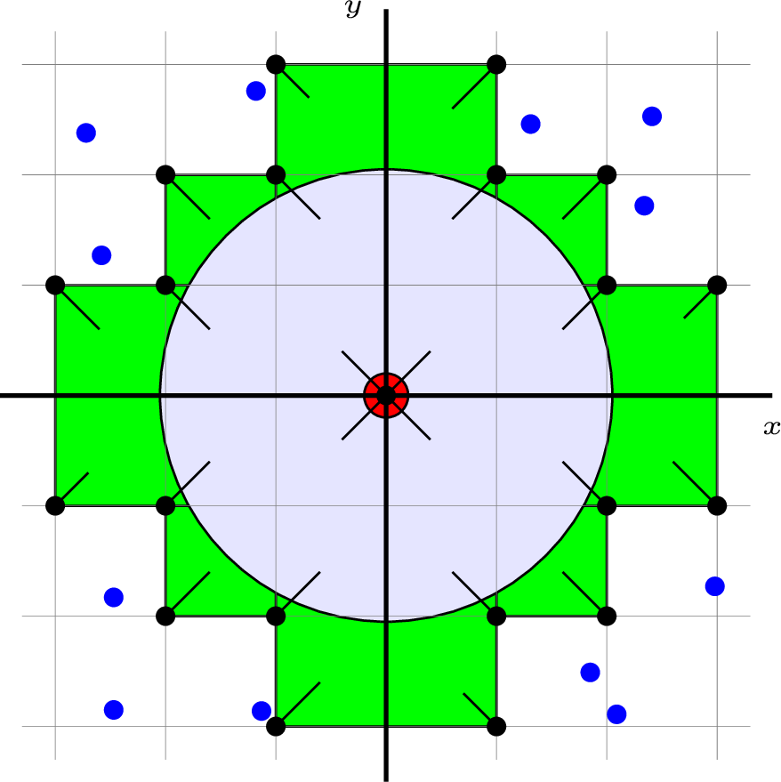
For that we set for any \((i,j)\in \{-1,0\}^2\), \(P_{i,j} =(0,0),\) and we define \(P_{0,1} = (1,2)\), \(P_{0,2} = (1,3)\), \(P_{1,0} = (2,1)\), \(P_{1,1} = (2,2)\), \(P_{2,0} = (3,1)\).
In the other three quadrants, we similarly define three sets of five points by rotation, see Figure 4.
The set \(\mathcal{C}_0(\Gamma_{d,R}^{\texttt{CN}}(P))\) is then reduced to the four points \((-1,-1)\), \((-1,0)\), \((0,-1)\) and \((0,0)\) which concludes the proof.
3 Proof of Theorem 5 (\(R_{\min}\))↩︎
In this section, we determine the values of \(R_{\min}^{\texttt{CN}}(p)\) and \(R_{\min}^{\texttt{NN}}(p)\) for all \(p\in[1,\infty]\). To do this, we use the fact that the connected component of the origin is infinite if and only if it contains an infinite self-avoiding path starting from the origin, where a self-avoiding path \((u_k)_{0\leq k < n}\), with \(n\in\mathbb{N}\cup\{\infty\}\) (where, to be precise, \(\mathbb{N}= \{0,1,\dots\}\) denotes the set of non-negative integers), is a path that does not visit a vertex more than once, i.e.for any \(k\neq l\), \(u_k \neq u_l\). For \(k\in\mathbb{N}\), we denote by \(x_k\) (resp. \(y_k\)) the horizontal (resp.vertical) coordinate of \(u_k\).
3.1 Upper bounds↩︎
Let \(p\in[1,\infty]\).
3.1.0.1 Proof of \(R_{\min}^{\texttt{CN}}(p)\) and \(R^{\texttt{NN}}_{\min}(p) \leq \displaystyle\frac{1}{2}\).
We set, for \(k\in\mathbb{N}\), \[\begin{array}{ll} P_{2k,0}=(2k+\frac{1}{2},0), & P_{2k+1,0}=(2k+1,0),\\ P_{2k+1,-1}=(2k+\frac{3}{2},0), & P_{2k+2,-1}=(2k+2,0), \end{array}\] see Figure 5. The sequence \(u = (u_k)_{k \geq 0}\) defined, for any \(k\in\mathbb{N}\), by \[\begin{array}{ll} u_{4k}=(2k,0), & u_{4k+1}=(2k+1,0),\\ u_{4k+2}=(2k+1,-1), & u_{4k+3}=(2k+2,-1) \end{array}\] is then an infinite self-avoiding path of \(\Gamma_{p,R}^{\texttt{CN}}(P)\) and of \(\Gamma_{p,R}^{\texttt{NN}}(P)\).
![Figure 5: Construction of an infinite self-avoiding path of \Gamma_{p,R}^{\texttt{CN}}(P) and of \Gamma_{p,R}^{\texttt{NN}}(P) for R\geq1/2 and for any p\in[1,\infty]. The pattern that is repeated periodically is in red and the arrows indicate to which cell the points belong.](/article/2607.14062/_pdflatex/rbgodyhq.png "fig:")
3.1.0.2 Proof of \(R_{\min}^{\texttt{CN}}(p) \leq \displaystyle \frac{2}{1+2^{2-\frac{1}{p}}}\).
We denote \[f(p)=\left\{ \begin{array}{ll} \displaystyle \frac{2}{1+2^{2-\frac{1}{p}}} & \text{if } p\in[1,\infty), \\[0.5cm] \displaystyle \frac{2}{5} & \text{if } p=\infty. \end{array} \right.\]
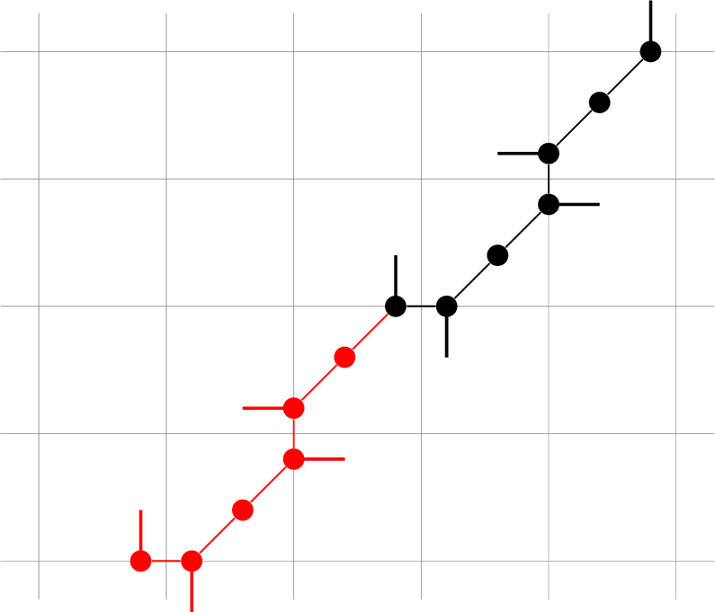
Consider the sequence \(u = (u_k)_{k \geq 0}\) defined, for any \(k\geq 0\), by \[\begin{array}{lll} u_{6k}=(2k,2k), & u_{6k+1}=(2k+1,2k-1), & u_{6k+2}=(2k+1,2k),\\ u_{6k+3}=(2k+2,2k), & u_{6k+4}=(2k+1,2k+1), & u_{6k+5}=(2k+2,2k+1). \end{array}\]
Let set the points of the concerned cells in such a way, for any \(k\geq 0\), \[\begin{array}{ll} P_{2k,2k}=\left(2k+1-\frac{f(p)}{2},2k\right), & P_{2k+1,2k-1}=\left(2k+1+\frac{f(p)}{2},2k\right), \\ P_{2k+1,2k}=\left(2k+1+\frac{2+f(p)}{4}, 2k + \frac{2-f(p)}{4}\right), &P_{2k+2,2k}=\left(2k+2,2k+1-\frac{f(p)}{2}\right), \\ P_{2k+1,2k+1}=\left(2k+2,2k+1+\frac{f(p)}{2}\right), & P_{2k+2,2k+1}=\left(2k+2 +\frac{2-f(p)}{4},2k+1+\frac{2+f(p)}{4}\right), \end{array}\] see Figure 6. Now, let us compute the distances between two consecutive points along the sequence \(u\). Using the symmetries, it is sufficient to compute only the two following distances: \[\begin{align} \|P_{0,0} - P_{1,-1}\|_p & = \|(f(p),0)\|_p \text{ and } \\ \|P_{1,0} - P_{1,-1}\|_p & = \bigg\|\bigg(\frac{2+f(p)}{4}-\frac{f(p)}{2},\frac{2-f(p)}{4}\bigg)\bigg\|_p\\ & = \bigg\|\bigg(\frac{2-f(p)}{4},\frac{2-f(p)}{4}\bigg)\bigg\|_p. \end{align}\]
For any \(p\in[1,\infty]\), those two distances are equal to \(f(p)\).
So \(u\) is an infinite self-avoiding path of \(\Gamma_{p,R}^{\texttt{CN}}(P)\) for \(R\geq f(p)\). On the other hand, it is not a path of \(\Gamma_{p,R}^{\texttt{NN}}(P)\) since the edge \((u_0,u_1) = \left((0,0),(1,-1)\right)\) is diagonal which is not an allowed edge.
3.1.0.3 Proof of the upper bound for \(R^{\texttt{NN}}_{\min}(p)\).
Unlike the two previous cases, the upper bound is a non explicit value defined as the unique solution of the equation \[\label{eq:RMINLocal} (2-R)^p + (3-3R)^p = (4R)^p\tag{1}\] for \(R\in[0,1]\).
Lemma 1.
Now, we present a self-avoiding path which gives us the lower bound for the nearest neighbor model when \(p\in \left[\ln(2)/\ln(4/3),\infty\right]\). For any \(p \in [1,\infty)\), Equation 1 has a unique solution in \([0,1]\), denoted by \(R(p)\). Furthermore, the function \(p\mapsto R(p)\) is decreasing on \([1,\infty)\); \(R(p)< 1/2\) for \(p> \ln(2)/\ln(4/3)\); and \(\lim_{p\to\infty} R(p)= 3/7\).
Proof. First, we prove that Equation 1 has a unique solution on the interval \([0,1]\). For any \(p \in [1,\infty)\), consider the function on \([0,1]\), \[g_p(R) = (4R)^p - (2-R)^p - (3-3R)^p = (4R)^p - \|2-R,3-3R\|_p^p.\]
Its derivative is \[g_p'(R) = 4^p p R^{p-1} + p (2-R)^{p-1} +3^p p(1-R)^{p-1}.\] It is positive on \([0,1]\). Hence, \(g_p\) is continuous and increasing, with \(g_p(0)= -2^p -3^p<0\) and \(g_p(1) = 4^p - 1 >0\). Hence, \(g_p(R)=0\) has a unique solution on \([0,1]\).
Now, let us prove that \(p\mapsto R(p)\) is decreasing on \([1,\infty)\). For any \(R\in[0,1]\) and \(1\leq p<q\), \(\|2-R,3-3R\|_p > \|2-R,3-3R\|_q\), by the inclusion of the ball for the \(\mathcal{L}^p-\)norm in the ball for the \(\mathcal{L}^q-\)norm. Hence, \(4R(p) = \|2-R(p),3-3R(p)\|_p > \|2-R(p),3-3R(p)\|_q\) which implies that \(g_q(R(p))>0\), and so \(R(q) < R(p)\).
Let us now prove that \(\displaystyle R \left(\frac{\ln(2)}{\ln\left(\frac{4}{3}\right)}\right)=\frac{1}{2}\). Let \(p\in[1,\infty)\) be such that \(R(p)=\frac{1}{2}\). Then, \(\left(\frac{3}{2}\right)^p + \left(\frac{3}{2}\right)^p = 2^p\), so that \(2 = \left(\frac{4}{3}\right)^p\).
Since \(p\mapsto R(p)\) is decreasing on \([1,\infty)\) with \(R(p) > 0\), the limit \(L=\lim_{p\to\infty}R(p)\) exists. It satisfies \(4L = \|2-L,3-3L\|_{\infty}\). By the above, \(L<1/2\), and if \(R<1/2\), \(2-R > 3-3R\), then \(4L = 3-3L\), which implies that \(L = 3/7\). ◻
We denote \(R(\infty)=3/7\). For any \(p \in [1,\infty]\), we set the points: \[\begin{array}{ll} P_{0,0}=\left(\frac{R(p)}{2},0\right), & P_{0,-1}=\left(\frac{1}{2}+\frac{R(p)}{4},-\frac{3}{4} + \frac{3R(p)}{4}\right),\\ P_{1,-1}=\left(1,-\frac{3}{2} + \frac{3R(p)}{2}\right), & P_{1,-2}=\left(1,-\frac{3}{2}+ \frac{R(p)}{2}\right). \end{array}\] which are represented by the red pattern in Figure 7. From these 4 points, we apply 3 transformations that are combinations of symmetries and rotations to obtain the 3 other colored patterns in Figure 7. Finally, the remaining points are obtained by applying translations of vector \((0,4k)\) for \(k\in\mathbb{N}\) to those 16 points.
Now, let us check that the distances between two consecutive points along the sequence thus obtained are less than \(R(p)\). For that, we only need to compute the two following distances \[\begin{align} \|P_{1,-1} - P_{1,-2}\|_p & = \|(0,R(p))\|_p = R(p) \text{ and } \\ \|P_{0,-1} - P_{0,0}\|_p & = \left\|\left(-\frac{1}{2}+\frac{R(p)}{4},-\frac{3}{4}+\frac{3R(p)}{4}\right)\right\|_p \\ & = \left\{ \begin{array}{ll} \displaystyle \left( \left(\frac{2-R(p)}{4}\right)^p + \left(\frac{3-3R(p)}{4}\right)^p\right)^{\frac{1}{p}} & ifp\in[1,\infty),\\[0.5cm] \displaystyle \max\left\{\frac{11}{28},\frac{12}{28}\right\} & ifp=\infty.\\ \end{array} \right. \\ & = R(p). \end{align}\]
The path \(u\) obtained from those points is thus an infinite self-avoiding path of \(\Gamma_{p,R}^{\texttt{NN}}(P)\) for \(R\geq R(p)\), see Figure 7.

3.2 Forbidden paths↩︎
We now address the lower bound. Since \(R_{\min}^{\texttt{CN}}(p)\leq 1/2\) and \(R_{\min}^{\texttt{NN}}(p)\leq 1/2\) for any \(p\geq1\), we assume that \(R<1/2\). For a path \((u_k)_{0\leq k\leq n}\), we denote by \(s_k = u_k - u_{k-1}\) the step from \(u_{k-1}\) to \(u_{k}\), for \(1\leq k\leq n\). Given that \(R<1/2\), it follows that \[\forall k\in\{1,\ldots,n\}, \quad s_{k}\in\mathcal{E}=\{\swarrow,\leftarrow,\nwarrow,\downarrow,\uparrow,\searrow,\rightarrow,\nearrow\},\] where each arrow represents the corresponding vector in \(\{-1,0,1\}^2\setminus\{(0,0)\}\) (for example \(\rightarrow= (1,0)\) and \(\swarrow=(-1,-1)\)).
The following lemma gives a necessary condition for a path to belong to \(\Gamma_{p,R}^{\texttt{CN}}(P)\) or to \(\Gamma^{\texttt{NN}}_{p,R}(P)\).
Lemma 2. Let \(a,b\in \mathbb{Z}_{>0} = \{1,2,\dots\}\), let \(R \in (0, a/b)\), and let \(u_0,\ldots,u_n\in\mathbb{Z}^2\). If there exists \(P\in\mathcal{P}\) such that \(u=(u_0,\ldots,u_n)\) is a path of \(\Gamma_{p,R}^{\texttt{CN}}(P)\) (resp.of \(\Gamma^{\texttt{NN}}_{p,R}(P)\)), then \[\forall k\in \{0,\ldots, n-b\}, \quad \|u_{k+b}-u_k\|_\infty \leq a.\]
Proof. It is enough to prove the result for \(k=0\). Assume that for all \(l\in\{0,\ldots,b-1\}\), \(\|P_{u_{l+1}}-P_{u_{l}}\|_p\leq R\). Then \(|X_{u_{l+1}}-X_{u_{l}}|\leq R\), and it follows that \(|X_{u_b} - X_{u_0}|\leq bR< a.\) Consequently, \(|x_b-x_0|<a+1\), so that \(|x_b-x_0|\leq a\). Similarly, \(|y_b - y_0|\leq a\). ◻
Lemma 2 allows us to display patterns that cannot appear in a path. In the rest of the article, we apply it in three cases.
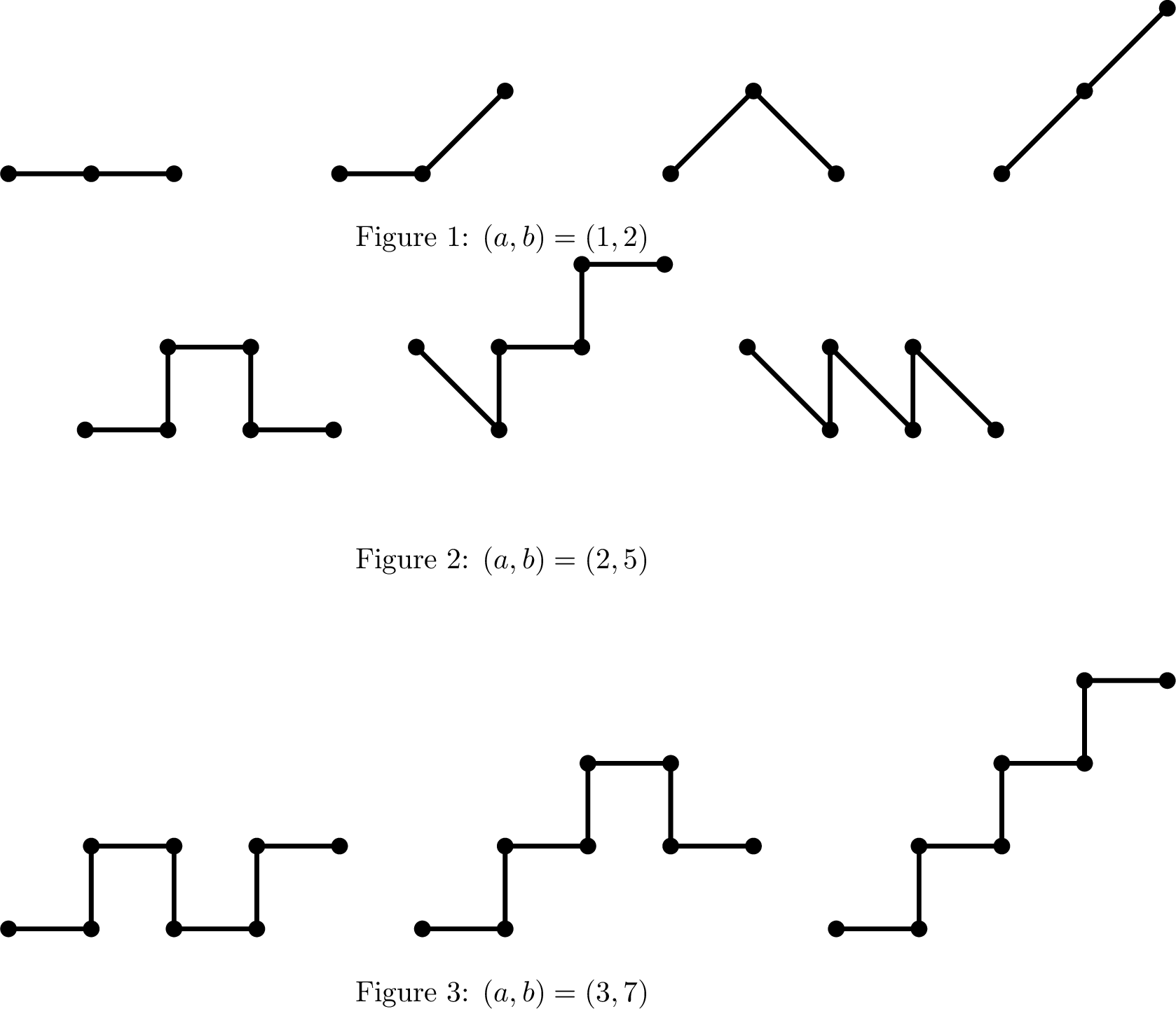
\((a,b)=(1,2)\), see Figure [fig:R601472] for a list of forbidden patterns when \(R<1/2\).
This case is used for all the lower bounds of Section 3.3.\((a,b)=(2,5)\), see Figure [fig:R602475] for some examples of forbidden patterns when \(R<2/5\).
This case is used for the lower bound of \(R_{\min}^{\texttt{CN}}(\infty)\) in Section 3.3.1.\((a,b)=(3,7)\), see Figure [fig:R603477] for some examples of forbidden patterns when \(R<3/7\).
This case is used for the lower bound of \(R_{\min}^{\texttt{NN}}(\infty)\) in Section 3.3.2.
3.3 Lower bounds↩︎
We distinguish two separate cases for each model: \(p=\infty\) and \(p\in[1,\infty)\). For \(p=\infty\), the proof consists in listing all possible beginnings of valid self-avoiding paths and showing that it is impossible to construct an infinite one, using Lemma 2. For \(p\in[1,\infty)\), we assume that there exists an infinite self-avoiding path and show that a given positive quantity decreases at least linearly along this path, which leads to an absurdity.
3.3.1 Complete neighbor model and \(p=\infty\)↩︎
Let \(u = (u_k)_{k \geq 0}\) be an infinite self-avoiding path of \(\Gamma_{\infty,R}^{\texttt{CN}}(P)\), for some \(R<2/5\). By symmetry, we assume without loss of generality that \(s_1\in\{\rightarrow, \nearrow\}\).
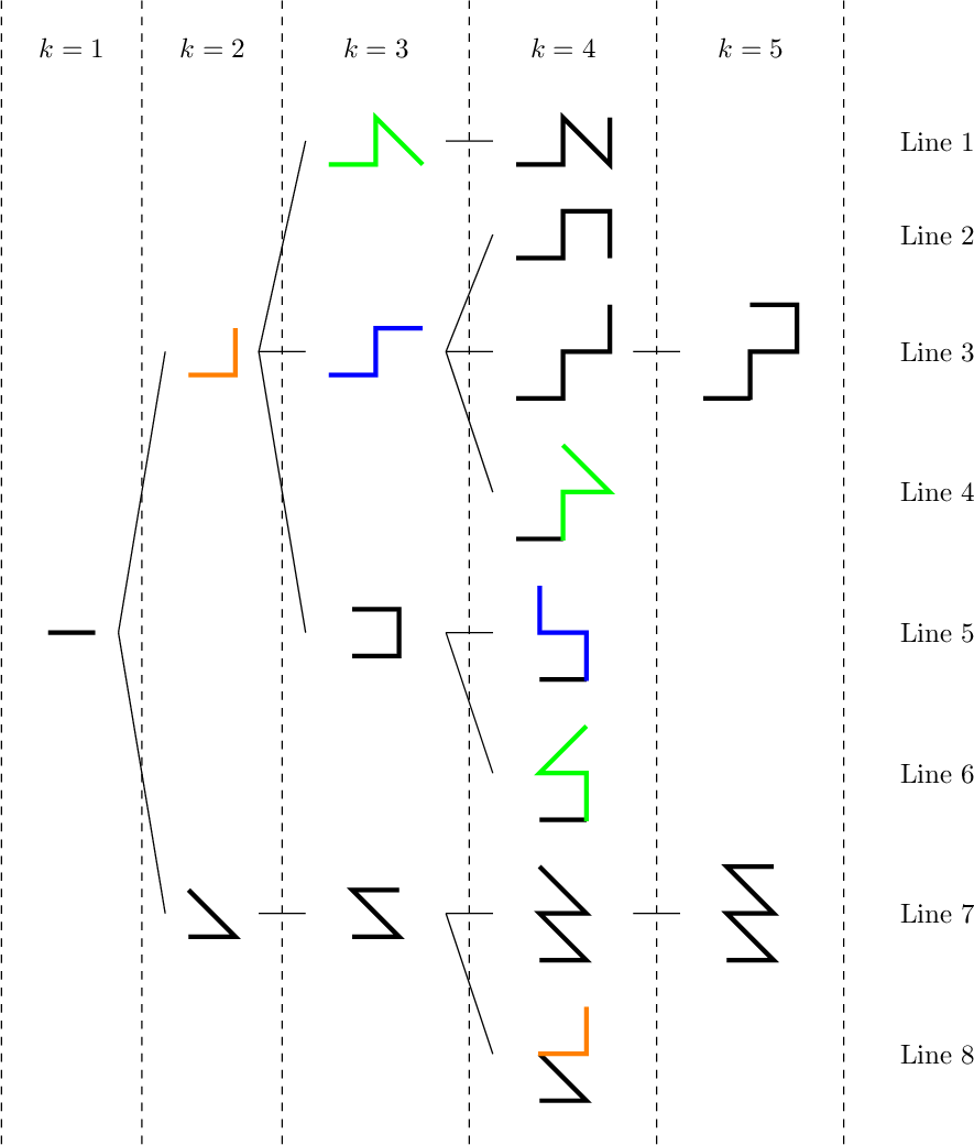
To begin with, let us examine the case \(s_1=\rightarrow\). By Lemma 2(i), \(s_2\notin\{\searrow,\rightarrow,\nearrow\}\). By symmetry, we assume that \(s_2 \in \{\nwarrow,\uparrow\}\). Figure 9 summarizes the case distinction that follows.
Case \(s_2=\uparrow\). By Lemma 2(i), \(s_3\notin\{\nwarrow,\uparrow,\nearrow\}\) and since \(u\) is self-avoiding, \(s_3\notin\{\swarrow,\downarrow\}\). So, \(s_3\in\{\searrow,\rightarrow,\leftarrow\}\).
Case \(s_3=\searrow\). By Lemma 2(i), \(s_4\notin\{\swarrow,\downarrow,\searrow,\rightarrow,\nearrow\}\) and since \(u\) is self-avoiding, \(s_4\notin\{\leftarrow,\nwarrow\}\). It follows that \(s_4=\uparrow\). Let us now examine the possible values for \(s_5\).
If \(s_5\in\{\swarrow,\leftarrow,\downarrow\}\), \(u\) is not self-avoiding.
If \(s_5\in\{\nwarrow,\uparrow,\nearrow\}\), by Lemma 2(i), \(u\) is not valid.
If \(s_5\in\{\searrow,\rightarrow\}\), by Lemma 2(ii), \(u\) is not valid.
So, there is no allowed value for \(s_5\). Consequently, the pattern \((\rightarrow,\uparrow,\searrow)\) and all the patterns derived from it by symmetry or rotation (“green” patterns, see Figure 9) are forbidden in \(u\).
For the rest of the proof, we make implicit the uses of the self-avoiding property and of Lemma 2(i).
Case \(s_3=\rightarrow\). Then, \(s_4\in\{\downarrow,\uparrow,\nwarrow\}\).
If \(s_4=\downarrow\), then by Lemma 2(ii), \(u\) cannot be extended.
If \(s_4=\uparrow\), then \(s_5=\leftarrow\), and by Lemma 2(ii), \(u\) cannot be extended.
If \(s_4=\nwarrow\), then \(u\) contains the green pattern \((\uparrow,\rightarrow,\nwarrow)\), which is forbidden, see Line 4 of Figure 9.
So, there is no allowed value for \(s_4\). Consequently, the pattern \((\rightarrow,\uparrow,\rightarrow)\) and all the patterns derived from it by symmetry or rotation (“blue” patterns, see Figure 9) are forbidden in \(u\).
Case \(s_3=\leftarrow\). Then \(s_4\in\{\uparrow,\nearrow\}\).
If \(s_4=\uparrow\), then \(u\) contains a blue pattern, which is forbidden, see Line 5 of Figure 9.
If \(s_4=\nearrow\), then \(u\) contains a green pattern, which is forbidden, see Line 6 of Figure 9.
So, there is no allowed value for \(s_4\).
Consequently, if \(s_1=\rightarrow\) and \(s_2=\uparrow\), there is no valid way to extend the path. It follows that the pattern \((\rightarrow,\uparrow)\) and all the patterns derived from it by symmetry or rotation (“orange” patterns, see Figure 9) are forbidden in \(u\).
Case \(s_2 = \nwarrow\). Then \(s_3=\rightarrow\). We have \(s_4\in\{\uparrow,\nwarrow\}\).
Finally, we obtain that \(u\) cannot begin by \(s_1=\rightarrow\), and more generally, that an infinite self-avoiding path of \(\Gamma_{\infty,R}^{\texttt{CN}}(P)\) cannot contain any horizontal or vertical edges. But, by Lemma 2(i), having two consecutive diagonal edges is forbidden. So, we conclude that \(u\) must be finite for any \(R<2/5\).
3.3.2 Nearest neighbor model and \(p=\infty\)↩︎
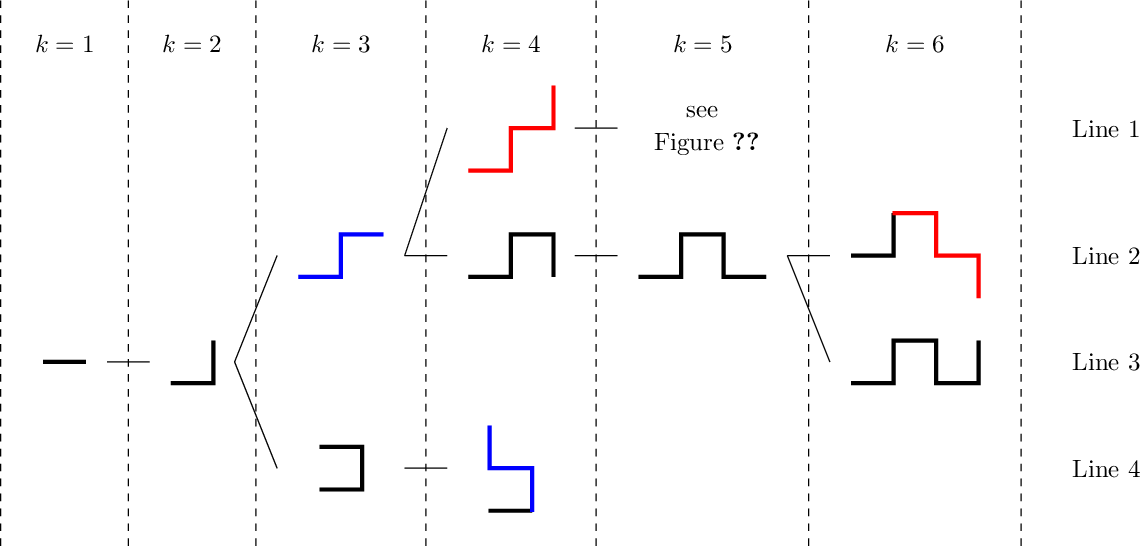
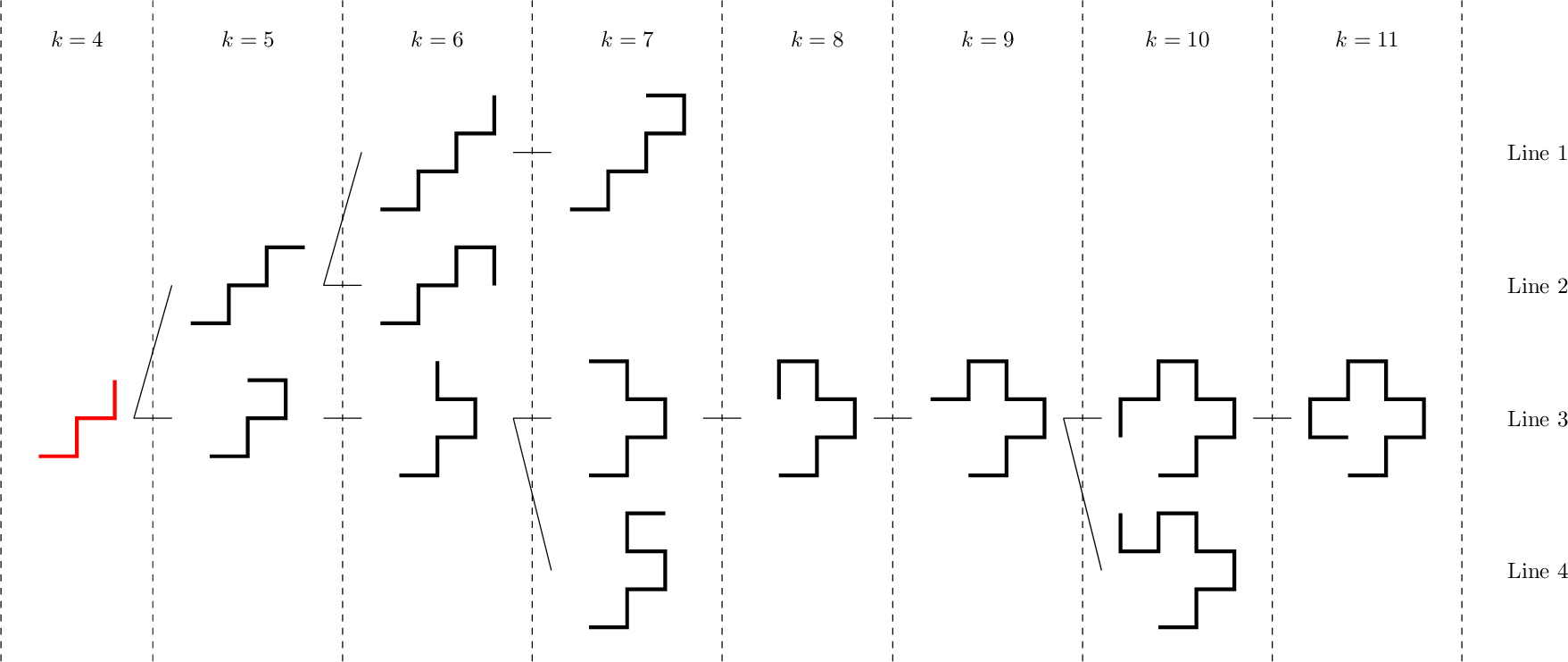
Let \(u = (u_k)_{k \geq 0}\) be an infinite self-avoiding path of \(\Gamma_{\infty,R}^{\texttt{NN}}(P)\), for some \(R<3/7\). By definition of the model, \(s_k\in\{\leftarrow,\downarrow,\uparrow,\rightarrow\}\) for all \(k\geq 0\). Furthermore, by Lemma 2(i), horizontal and vertical steps alternate in \(u\). We assume without loss of generality that \((s_1,s_2)=(\rightarrow,\uparrow)\), which implies that for all \(k\geq0\), \(s_{2k+1}\in\{\leftarrow,\rightarrow\}\) and \(s_{2k+2}\in\{\downarrow,\uparrow\}\). For the rest of the proof, we make implicit the use of the self-avoiding property and of Lemma 2(i). Figures 10 and 11 summarize the case distinction that follows.
Case \((s_3,s_4)=(\rightarrow,\uparrow)\).
Case \((s_5,s_6)=(\rightarrow,\uparrow)\). By Lemma 2(iii), we must then have \(s_7=\leftarrow\), see Line 1 of Figure 11. By applying Lemma 2(iii) once again, we obtain that \(u\) cannot be extended.
Case \((s_5,s_6)=(\rightarrow,\downarrow)\). By Lemma 2(iii), \(u\) cannot be extended, see Line 2 of Figure 11.
Case \(s_5=\leftarrow\). For the study of this case, we refer to Figure 11 (Lines 3 and 4), that examines the different ways to continue the path, and shows that they all eventually reach a stage where they can no longer be extended.
Consequently, the pattern \((\rightarrow,\uparrow,\rightarrow,\uparrow)\) and all the patterns derived from it by symmetry or rotation (“red” patterns, see Figure 10 and 11) are forbidden in \(u\).
Case \((s_3,s_4)=(\rightarrow,\downarrow)\). We have \(s_5=\rightarrow\). If \(s_6=\downarrow\), then \(u\) contains a red pattern, which is forbidden, see Line 2 of Figure 10. So, \(s_6=\uparrow\). By Lemma 2(iii), \(u\) cannot be extended, see Line 3 of Figure 10.
Consequently, the pattern \((\rightarrow,\uparrow,\rightarrow)\) and all the patterns derived from it by symmetry or rotation (“blue” patterns, see Figure 10) are forbidden in \(u\).
- Case \(s_3=\leftarrow\). Then, \(s_4=\uparrow\). But \(u\) contains a blue pattern, which is forbidden, see Line 4 of Figure 10.
We conclude that for \(R<3/7\), \(u\) must be finite which implies that \(R_{\min}\geq 3/7\).
3.3.3 Complete neighbor model and \(p\in[1,\infty)\)↩︎
For \(p\in[1,\infty)\), the proof requires more subtle arguments: let \(R < \displaystyle\min \left\{\frac{1}{2},\frac{2}{1+2^{2-\frac{1}{p}}}\right\}\) and let \(u=(u_k)_{k\geq0}\) be an infinite self-avoiding path of \(\Gamma_{p,R}^{\texttt{CN}}(P)\) for some \(P\in\mathcal{P}\). We construct a subsequence \((u_{a_k})_{k\geq1}\), and we study the distance \(A_k\) from the point \(P_{u_{a_k}}\) to a certain border of the cell to which it belongs. We prove that \((A_k)_{k\geq0}\) decreases at least linearly and becomes negative, which leads to a contradiction. This implies that the sequence \(u\) must be finite.
3.3.3.1 Notations.
Let us denote by \(\mathcal{D}=\{\swarrow,\nwarrow,\searrow,\nearrow\}\) the set of diagonal edges. We suppose that \(u\) is a self-avoiding path of \(\Gamma_{p,R}^{\texttt{CN}}(P)\), and we define the sequence \((a_k)_{k\geq1}\) by
\(a_1 = \left \{ \begin{array}{ll} 1 if s_2\notin \mathcal{D},\\ 2 otherwise. \end{array} \right.\)
for \(k\geq1\), \(a_{k+1} = \left \{ \begin{array}{ll} a_k + 2 if \|u_{a_k+5}-u_{a_k}\|_{\infty} \neq 3,\\ a_k + 3 otherwise. \end{array} \right.\)
From the sequence \((a_k)_{k \geq 1}\), we define, for any \(k \geq 1\), \[\delta_{k} = \left \{ \begin{array}{ll} s_{a_{k} +2} & ifs_{a_{k} +2}\notin \mathcal{D},\\ s_{a_{k} +1} + s_{a_{k} +2} & otherwise. \end{array} \right.\]
One can prove, using Lemma 2(i), that, for any \(k \geq 1\), \(\delta_k \in \{\leftarrow,\rightarrow,\downarrow,\uparrow\}\).
Moreover, for any \(k \geq 1\), we define \[\label{eq:Ak} A_k = \left\{ \begin{array}{ll} X_{u_{a_k}}-x_{u_{a_k}} & { if } \delta_k = \rightarrow,\\ 1+x_{u_{a_k}}-X_{u_{a_k}} & { if } \delta_k = \leftarrow,\\ Y_{u_{a_k}}-y_{u_{a_k}} & { if } \delta_k = \uparrow,\\ 1+y_{u_{a_k}}-Y_{u_{a_k}} & { if } \delta_k = \downarrow. \end{array} \right.\tag{2}\]
The quantity \(A_k\) represents the distance between \(P_{u_{a_k}}\) and the border of its cell specified by \(\delta_k\). More precisely, if \(\delta_k=\rightarrow\), \(A_k\) is the distance between \(P_{u_{a_k}}\) and the left border of its cell, while if \(\delta_k=\downarrow\), it is the distance with the top border, and similarly for the other possible directions, see Figure 12 for an illustration.
Our aim is to control the increment \(A_{k+1}-A_k\). To this end, we first look at the possible patterns we can observe between the points \(u_{a_k}\) and \(u_{a_{k+1}}\).

3.3.3.2 List of patterns between \(u_{a_k}\) and \(u_{a_{k+1}}\).
Let \(k\geq1\). We identify all the possible patterns between \(u_{a_k}\) and \(u_{a_{k+1}}\), and control the value of \(A_{k+1}-A_k\) accordingly.
In all that follows, we use implicitly the self-avoiding property and Lemma 2(i).
Without loss of generality, we only consider the two cases \(s_{a_{k}+1}=\rightarrow\) and \(s_{a_{k}+1} = \nearrow\). Let us first treat the case \(s_{a_{k}+1} = \rightarrow\). By symmetry, we can assume that \(s_{a_k}\in\{\nwarrow,\uparrow\}\). If \(s_{a_k}=\uparrow\), we have \(s_{a_k+2}\in\{\nwarrow,\downarrow,\uparrow\}\), and if \(s_{a_k}=\nwarrow\), then \(s_{a_k+2}\in\{\swarrow,\nwarrow,\uparrow\}\).
Figure 13 displays all of these possible scenarios. In the following, we use a letter together with one or several numbers to refer to the corresponding cells on Figure 13.
Le us start by examining the possibilities described on the left table of Figure 13, which correspond to the case where \(s_{a_k+2}\in\{\nwarrow,\uparrow\}\).
(A.2,3,4) Case \(s_{a_k+2} = \nwarrow\). Then \(s_{a_k+3}=\rightarrow\). Since we have \(\|u_{a_{k}+3}-u_{a_k}\|_{\infty} = 1\) and \(\|u_{l+2}-u_{l}\|_{\infty}=1\) for any \(l\geq1\), we obtain that \(\|u_{a_{k}+5}-u_{a_k}\|_{\infty}\leq 2\). So \(a_{k+1}=a_k+2\).
(B.2) Case \(s_{a_k+2} = \uparrow\). Then \(s_{a_k+3}\in\{\leftarrow,\searrow,\rightarrow\}\).
(B.3,4) If \(s_{a_k+3}=\leftarrow\), we have \(\|u_{a_{k}+3}-u_{a_k}\|_{\infty} = 1\). So \(a_{k+1}=a_k+2\).
(C.3,4,5) If \(s_{a_k+3}=\searrow\), then \(s_{a_k+4}=\uparrow\). It implies that \(s_{a_k+5}\in\{\searrow,\rightarrow\}\). So \(\|s_{a_{k}+5}-s_{a_k}\|_\infty=3\) and \(a_{k+1}=a_k+3\).
(D.3) If \(s_{a_k+3}=\rightarrow\), then \(s_{a_k+4}\in\{\nwarrow,\downarrow,\uparrow\}\).
(D.4,5) If \(s_{a_k+4} = \nwarrow\), then \(s_{a_k+5} = \rightarrow\). We have \(\|s_{a_{k}+5}-s_{a_k}\|_\infty=2\), so \(a_{k+1}=a_k+2\).
(E.4) If \(s_{a_k+4} = \uparrow\), then \(s_{a_k+5} \in\{\leftarrow,\searrow,\rightarrow\}\).
(E.5) If \(s_{a_k+5}\in\{\searrow,\rightarrow\}\), then \(\|s_{a_{k}+5}-s_{a_k}\|_{\infty}=3\), so we have \(a_{k+1}=a_k+3\).
(F.5) If \(s_{a_k+5}=\leftarrow\), then \(\|s_{a_{k}+5}-s_{a_k}\|_{\infty}=2\), so we have \(a_{k+1}=a_k+2\).
(G.4,5) If \(s_{a_k+4} = \downarrow\), then \(s_{a_k+5} \in\{\rightarrow,\nearrow\}\) and we have \(\|s_{a_{k}+5}-s_{a_k}\|_{\infty}=3\), so we have \(a_{k+1}=a_k+3\).
For the study of the case \((s_{a_k},s_{a_k+2})\in\left\{\left(\nwarrow,\swarrow\right),\left(\uparrow,\downarrow\right)\right\}\), we refer to the right table of Figure 13. Let us only mention that if \((s_{a_k},s_{a_k+1},s_{a_k+2}) = (\nwarrow,\rightarrow,\swarrow)\), which corresponds to cell (A’.2), the path cannot be extended, so that we can exclude this case.

The above analysis shows that if \(s_{a_k+1}\notin \mathcal{D}\) then \(s_{a_{k+1}+1}\notin \mathcal{D}\). Furthermore, by Lemma 2(i), if \(s_2 \in \mathcal{D}\), then \(s_3 \notin \mathcal{D}\). Therefore, in all cases, we have \(s_{{a_1}+1}\notin \mathcal{D}\). By induction, it follows that for all \(k\geq1\), \(s_{a_{k}+1}\notin \mathcal{D}\). Hence, we can exclude the case \(s_{a_{k}+1}= \nearrow\).
Furthermore, the observation of the two tables of Figure 13 shows that, whatever the pattern to which \(s_{a_k}\) belongs, the evolution from \(s_{a_{k+1}}\) is then given by the left table (see the possible steps after \(s_{a_{k+1}}\) in columns \((4)\) and \((5)\) of the two tables). By induction, this means that for \(k\geq2\), up to a rotation or symmetry, we always have \[\label{eq:uShape} (s_{a_{k+1}},s_{a_{k+1}+1},s_{a_{k+1}+2}) \in\{\nwarrow,\uparrow\}\times\{\rightarrow\}\times\{\nwarrow,\uparrow\}.\tag{3}\]
Moreover, for \(k\geq2\),
if \(a_{k+1} - a_k = 2\), then \(y_{u_{a_{k+1}}}-y_{u_{a_k}}=1\) and \(\delta_{k+1}=\delta_k=\uparrow\), see cells (A.4), (B.4), (D.5), (F.5) of Figure 13;
if \(a_{k+1} - a_k = 3\), then \(s_{a_k+2} = \uparrow\), \(s_{a_{k}+3}\in\{\nwarrow,\uparrow\}\) and \(\delta_{k+1}=\rightarrow\), see cells (C.5), (E.5), (G.5) of Figure 13.
To conclude the proof, let us now show that there exists a constant \(c>0\) such that for all \(k\geq2\), we have \[A_{k+1} - A_k\leq-\min\{1-2R,c\}<0.\]
For that, we consider separately the cases \(a_{k+1}-a_k=2\) and \(a_{k+1}-a_k=3\). As before, we assume without loss of generality that equation 3 is satisfied.
3.3.3.3 Case \(a_{k+1}-a_k=2\).
From the above, we have \(y_{u_{a_{k+1}}}-y_{u_{a_k}}=1\) and \(\delta_{k+1}=\delta_k=\uparrow\). Thus, \[A_{k+1} - A_k = (Y_{u_{a_{k+1}}}-y_{u_{a_{k+1}}}) - (Y_{u_{a_k}}-y_{u_{a_k}}) = Y_{u_{a_{k+1}}} - Y_{u_{a_k}} -1.\] Since \(a_{k+1}=a_k+2\), it follows that \(Y_{u_{a_{k+1}}}\leq Y_{u_{a_k}} + 2R\). So, \[A_{k+1} - A_k \leq -(1-2R)<0.\]
3.3.3.4 Case \(a_{k+1}-a_k = 3\).
As in Section 3.1, we set \(\displaystyle f(p) = \frac{2}{1+2^{2-\frac{1}{p}}}\).
From the above, we have \((s_{a_k},s_{a_k+1},s_{a_k+2},s_{a_k+3})\in\{\nwarrow,\uparrow\}\times\{\rightarrow\}\times\{\uparrow\}\times\{\searrow,\rightarrow\}\), see Figure 14.
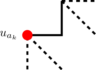
We assume without loss of generality that \(u_{a_k} = (0,0)\), which implies that \(u_{a_k+2} = (1,1)\), \(A_{k+1} = X_{u_{a_{k+1}}}-2\) and \(A_k = Y_{0,0}\). Since \(u\) is a path of \(\Gamma_{p,R}^{\texttt{CN}}(P)\), we have \[\|P_{1,1} - P_{0,0}\|_p^p = (X_{1,1}-X_{0,0})^p + (Y_{1,1}-Y_{0,0})^p \leq (2R)^p.\]
Using \(X_{0,0}\in[0,1]\) and \(Y_{1,1}\in[1,2]\), we obtain \[(X_{1,1}-1)^p + (1-Y_{0,0})^p \leq (2R)^p.\]
It follows that \[\label{eq:StairsIneq} X_{1,1} \leq 1 + \big[(2R)^p - (1-Y_{0,0})^p\big]^{\frac{1}{p}}.\tag{4}\]
Since \(X_{u_{a_{k+1}}}\leq X_{1,1} + R\), it implies that \[\begin{align} A_{k+1}-A_k & \leq X_{1,1}+R-2-Y_{0,0} \\ & \leq \big[\big(2R\big)^p - (1-Y_{0,0})^p\big]^{\frac{1}{p}} +R-1-Y_{0,0} \\ & < \big[\big(2f(p)\big)^p - (1-Y_{0,0})^p\big]^{\frac{1}{p}} +f(p)-1-Y_{0,0} \text{ (because R< f(p)).} \end{align}\]
Observe that \(Y_{0,0}\in[0,R]\) because \(s_{a_k} \in \{\nwarrow,\uparrow\}\). To conclude, we show that for all \(x\in[0,R]\), the following inequality holds: \[(2f(p))^p\leq (1+x-f(p))^p + (1-x)^p.\]
To this purpose, we introduce the function \(g(x) = (1+x-f(p))^p + (1-x)^p\), for \(x\in[0,R]\). By studying its derivative, we obtain that \(g\) admits a minimum in \(f(p)/2\). Thus, for all \(x\in[0,R]\), \[g(x)\geq g\bigg(\frac{f(p)}{2}\bigg) =2\bigg(1-\frac{f(p)}{2}\bigg)^p=(2f(p))^p.\]
As a consequence, we obtain that, for any \(Y_{0,0} \in [0,R]\), \[\big[\big(2R\big)^p - (1-Y_{0,0})^p\big]^{\frac{1}{p}} +R-1-Y_{0,0} < 0.\] Since \([0,R]\) is compact, there exists \(c>0\) such that \(A_{k+1}-A_k \leq -c.\)
3.3.3.5 Conclusion:
For any \(k\geq 2\), we have \(A_{k+1}-A_k \leq -\min\{1-2R,c\} < 0\). Since \((A_k)_{k\geq 0}\) is a sequence of positive real number, this leads to a contradiction. Consequently, for \(R<\min\left\{\frac{1}{2},\frac{2}{1+2^{2-\frac{1}{p}}}\right\}\), the graph \(\Gamma_{p,R}^{\texttt{CN}}(P)\) does not contain any infinite self-avoiding path.
3.3.4 Nearest neighbor model and \(p\in[1,\infty)\)↩︎
Let \(p\in\big[1,\infty\big)\), \(R< \min\{1/2,R(p)\}\) and let \(u=(u_k)_{k\geq0}\) be an infinite self-avoiding path of \(\Gamma_{p,R}^{\texttt{NN}}(P)\) for some \(P\in\mathcal{P}\). We now have \(s_k=u_k-u_{k-1}\in\{\leftarrow,\downarrow,\uparrow,\rightarrow\}\) for \(k\geq1\).
3.3.4.1 Staircase pattern.
We introduce the set \(\mathcal{S}=\{n\geq1 : s_n=s_{n+2} and s_{n+1} = s_{n+3}\}\), which contains positions at which the path presents a staircase pattern of length at least 4. We first prove the following.
Lemma 3. The set \(\mathcal{S}\) is infinite.
Proof. Let us assume by contradiction that \(\mathcal{S}\) is finite, and let \(M=\max\mathcal{S}\), with the convention that \(M=0\) if \(\mathcal{S}=\emptyset\). Even if it means replacing \(u\) by \((u_k)_{k\geq M}\), we can assume without loss of generality that \(\mathcal{S}=\emptyset\). Up to a rotation and a symmetry, we may also assume that \((s_1,s_2)=\left(\rightarrow,\uparrow\right)\), by Lemma 2(i). We have then \(s_3\in\{\leftarrow,\rightarrow\}\).
If \(s_3=\leftarrow\), the self-avoiding property and Lemma 2(i) imply that \(s_4=\uparrow\). Then, since \(\mathcal{S}=\emptyset\), we have \(s_5=\rightarrow\), and by induction, we obtain that \(s_{2k+2}=\uparrow\) and \((s_{4k+1},s_{4k+3})=(\rightarrow,\leftarrow)\) for all \(k\geq 0\). Let us set \(D_k = Y_{u_{2k}} - y_{u_{2k}}\), for \(k\geq 0\). This quantity represents the distance of the points \(P_{u_{2k}} = (X_{u_{2k}},Y_{u_{2k}})\) to the bottom border of their cells. We have \(Y_{u_{2k}+2}\leq Y_{u_{2k}} +2R\) and \(y_{u_{2k}+2} = y_{u_{2k}} +1\), so that \(D_{k+1}-D_k \leq -(1-2R)<0\). Since \(D_k>0\) for all \(k\geq 0\), this leads to a contradiction.
If \(s_3=\rightarrow\), we obtain analogously that \(s_{2k+1}=\rightarrow\) and \((s_{4k+2},s_{4k+4})=(\uparrow,\downarrow)\) for all \(k\geq 0\), and we conclude in the same way with \(D_k = X_{u_{2k}} - x_{u_{2k}}\).
◻
3.3.4.2 Notations.
The rest of the proof follows the same approach as in Section 3.3.3. Using the fact that \(\mathcal{S}\) is infinite, we define a sequence \((a_k)_{k\geq1}\), with the help of two additional sequences \((n_k)_{k\geq1}\) and \((b_k)_{k\geq1}\).
The sequence \((n_k)_{k\geq1}\) is defined by
\(n_1 = \min \{n\geq 1 : n\in \mathcal{S}\}\),
for \(k\geq1\), \(n_{k+1} = \min \{n\geq n_k+2 : n\in \mathcal{S}\}\),
and the sequence \((b_k)_{k\geq1}\) by
\(b_1 = 1\),
for \(k\geq1\), \[\label{eq:b95k} b_{k+1} = \left\{ \begin{array}{ll} b_k +1 & { if } n_{b_k+1} - n_{b_k} \neq 3,\\ b_k +2 & { if } n_{b_k+1} - n_{b_k} = 3andn_{b_k+2} - n_{b_k+1} \neq 3,\\ b_k +3 & { if } n_{b_k+1} - n_{b_k} = 3andn_{b_k+2} - n_{b_k+1} = 3.\\ \end{array} \right.\tag{5}\]
For \(k \geq 1\), we set \(a_k=n_{b_k}\), \(\delta_k = s_{a_k}\), and we then define \(A_k\) as in Equation 2 .
3.3.4.3 List of patterns between \(u_{n_k}\) and \(u_{n_{k+1}}\).
Like in Section 3.3.3, we first describe the patterns observed between the points \(u_{n_k}\) and \(u_{n_{k+1}}\), and then give an upper bound for \(A_{k+1}-A_{k}\) in all the possible cases.
Lemma 4. Let \(k\geq1\) be such that \(s_{n_k}= s_{n_k+2}= \rightarrow\) and \(s_{n_k+1}= s_{n_k+3} = \uparrow\). Then,
if \(n_{k+1} - n_k = 2l\) with \(l\geq1\), then between the points \(u_{n_{k}+1}\) and \(u_{n_{k+1}+1}\), the path alternates between the patterns \((\rightarrow,\uparrow)\) and \((\rightarrow,\downarrow)\), i.e., \[\forall m\in\{2,\ldots, 2l+1\}, \quad s_{n_k + m} = \begin{cases} \rightarrow& \text{if } m = 0 \mod 2,\\ \downarrow& \text{if } m = 1 \mod 4,\\ \uparrow& \text{if } m =3 \mod 4. \end{cases}\]
if \(n_{k+1} - n_k = 2l+1\) with \(l\geq1\), then between the points \(u_{n_{k}+1}\) and \(u_{n_{k+1}+2}\), the paths alternates between the patterns \((\rightarrow,\uparrow)\) and \((\leftarrow,\uparrow)\), i.e., \[\forall m\in\{2,\ldots,2l+2\}, \quad s_{n_k + m} = \begin{cases} \uparrow& \text{if } m = 1 \mod 2,\\ \leftarrow& \text{if } m = 0 \mod 4,\\ \rightarrow& \text{if } m = 2 \mod 4. \end{cases}\]
In particular, for any \(k \geq 1\), \[s_{n_{k+1}} = \left\{ \begin{array}{ll} \rightarrow& ifn_{k+1} - n_kis even,\\ \uparrow& ifn_{k+1} - n_kis odd. \end{array} \right.\]
Proof. We use the same ideas as in the proof of Lemma 3. ◻
Figure 15 represents the patterns between \(u_{n_k}\) and \(u_{n_{k+1}}\) for \(n_{k+1} - n_k\) even (green path) and odd (blue path).

3.3.4.4 Two important lemmas.
For the rest of the proof, we use the two following lemmas.
Lemma 5. Let \(p\in[1,\infty)\) and \(R< \min\{1/2,R(p)\}\). We consider the sequence \(u=(u_k)_{0\leq k\leq6}\) defined by \[\begin{array}{llll} u_0 = (0,0), & u_1 = (1,0), & u_2 = (1,1), & u_3 = (2,1),\\ u_4 = (2,2), & u_5 = (1,2), & u_6 = (1,3),& \end{array}\] see Figure 16. Then, there exists \(c_1>0\) such that for any \(P\in\mathcal{P}\) such that \(u\) is a path of \(\Gamma_{p,R}^{\texttt{NN}}(P)\), we have \[\label{eq:odd} (Y_{1,3} - 3) - (X_{1,0} - 1) \leq -c_1 <0.\tag{6}\]
See Appendix 6.1 for the proof.
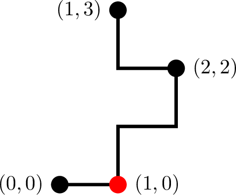
Lemma 6. Let \(p\in[1,\infty)\), \(R<\min\{1/2,R(p)\}\). We consider the sequence \(u=(u_k)_{0\leq k\leq9}\) defined by \[\begin{array}{llll} u_0 = (0,0), & u_1 = (1,0), & u_2 = (1,1), & u_3 = (2,1),\\ u_4 = (2,2), & u_5 = (1,2), & u_6 = (1,3), & u_7 = (0,3),\\ u_8 = (0,2), & u_9 = (-1,2), && \end{array}\] see Figure 17. Then, there exists \(c_2>0\) such that for any \(P\in\mathcal{P}\) such that \(u\) is a path of \(\Gamma_{p,R}^{\texttt{NN}}(P)\), we have \[\label{eqodd} (1 + (-1) - X_{-1,2}) - (X_{1,0}-1) \leq -c_2<0.\tag{7}\]
See Appendix 6.2 for the proof.
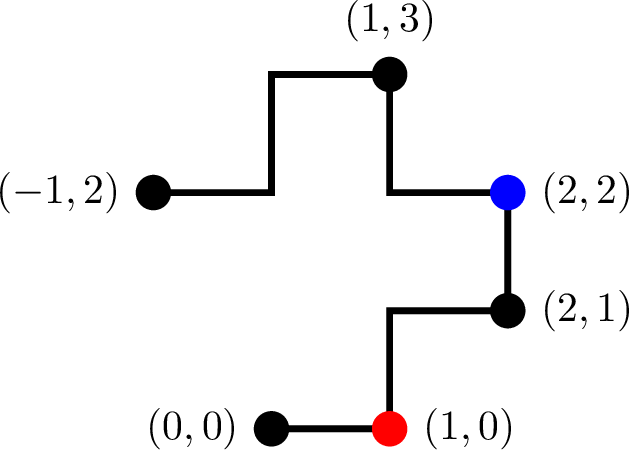
Lemmas 4, 5 and 6 are important and they permit, in the following, to upperbound \(A_{k+1}-A_k\).
Let \(k\geq1\) be fixed. We suppose without loss of generality that \(s_{a_k}=s_{a_k+2}=\rightarrow\) and \(s_{a_k+1}= s_{a_k+3} = \uparrow\).
3.3.4.5 Case \(b_{k+1}-b_k = 1\).
By Equation 5 , \(n_{b_{k}+1} - n_{b_k}\not=3\). We now distinguish the even case and the odd case.
Even case: \(n_{b_{k+1}} - n_{b_k} = 2l\) with \(l\geq1\).
Then point \(u_{a_{k+1}}\) is a green point on Figure 15. By Lemma 4, we have \(\delta_{k+1} = \delta_k = \rightarrow\) and \(x_{u_{a_{k+1}}}= x_{u_{a_{k}}} + l\). So, \(X_{u_{a_k+2l}} \leq X_{u_{a_k}} + 2lR\). We obtain then \[\begin{align} A_{k+1} - A_{k} &= (X_{u_{a_{k+1}}} - x_{u_{a_{k+1}}}) - (X_{u_{a_k}} - x_{u_{a_k}})\\ &\leq-2l\left(\frac{1}{2}-R\right) \leq -(1-2R) < 0. \end{align}\]Odd case: \(n_{b_{k+1}} - n_{b_k} = 2l+1\) with \(l\geq2\).
The point \(u_{a_{k+1}}\) is a purple point, except the first one (because \(l \geq 2\)), on Figure 15. To upperbound \(A_{k+1}-A_k\), we split this value into two terms. One is upperbound by Lemma 5 and the other one using Lemma 4. We have \[\begin{align} A_{k+1} - A_{k} &= (Y_{u_{a_{k+1}}} - y_{u_{a_{k+1}}}) - (X_{u_{a_k}} - x_{u_{a_k}})\\ &= (Y_{u_{a_{k}+2l+1}} -y_{u_{a_{k}+2l+1}}) - (Y_{u_{a_{k}+5}} - y_{u_{a_{k}+5}}) \\ & \quad + (Y_{u_{a_{k}+5}} - y_{u_{a_{k}+5}}) - (X_{u_{a_k}} - x_{u_{a_k}}).\\ \end{align}\]Up to a translation, \((u_l)_{a_k-1\leq l \leq a_{k+5}}\) satisfies the hypotheses of Lemma 5. It follows that \[(Y_{u_{a_{k}+5}} - y_{u_{a_{k}+5}}) - (X_{u_{a_k}} - x_{u_{a_k}}) \leq -c_1.\]
By applying Lemma 4 to \((u_l)_{l\geq a_{k+2}}\), we have \(y_{u_{a_{k}+2l+1}} = y_{u_{a_{k}+5}} + l-2\). Since \(u\) is a path of \(\Gamma_{p,R}^{\texttt{NN}}(P)\), it implies that \[Y_{u_{a_{k}+2l+1}} \leq Y_{u_{a_{k}+5}} + 2(l-2)R.\]
So, we obtain \[A_{k+1} - A_k \leq -2(l-2)\left(\frac{1}{2}-R\right) -c_1 \leq -c_1 < 0.\]
3.3.4.6 Case \(b_{k+1}-b_k = 2\).
By definition (see Equation 5 ), we have \(n_{b_k+1} - n_{b_k} = 3\) and either \(n_{b_k+2} - n_{b_k+1} = 2l\) with \(l\geq1\), or \(n_{b_{k}+2} - n_{b_k+1} = 2l+1\) with \(l\geq2\). Such configurations are represented on Figure 18.

Even case: \(n_{b_k+2} - n_{b_k+1} = 2l\) with \(l\geq1\).
The point \(u_{a_{k+1}}\) is a green point on Figure 18. As in the previous case (\(b_{k+1}-b_k = 1\), odd case), we obtain \[A_{k+1} - A_k \leq -2(l-1)\left(\frac{1}{2}-R\right)-c_1 \leq -c_1.\]Odd case: \(n_{b_k+2} - n_{b_k+1} = 2l+1\) with \(l\geq2\).
The point \(u_{a_{k+1}}\) is a purple point on Figure 18. By Lemma 4, we have \(A_{k+1} = 1+ x_{u_{a_{k+1}}}-X_{u_{a_{k+1}}}\). As previously, to upperbound \(A_{k+1}-A_k\), we split it into two terms. One is upperbounded by Lemma 6 and the other one using Lemma 4.\[\begin{align} A_{k+1} - A_k &= (1+x_{u_{a_{k+1}}}-X_{u_{a_{k+1}}} ) - (X_{{u_{a_k}}}-x_{{u_{a_k}}})\\ & = (1+x_{u_{a_{k+1}}}-X_{u_{a_{k+1}}}) - (1+ x_{u_{a_k+8}}-X_{u_{a_k+8}}) \\ & \quad + (1+x_{u_{a_k+8}}-X_{u_{a_k+8}}) - (X_{{u_{a_k}}}-x_{{u_{a_k}}}). \end{align}\]
Up to a translation, \((u_l)_{a_k-1\leq l \leq a_{k+8}}\) satisfies the hypotheses of Lemma 6. It follows that \[(1+ x_{u_{a_k+8}} -X_{u_{a_k+8}}) - (X_{{u_{a_k}}} - x_{{u_{a_k}}})\leq -c_2.\]
By Lemma 4, we have \(x_{u_{a_{k+1}}} = x_{u_{a_k+8}} - (l-2)\) which implies that \[(1+x_{u_{a_{k+1}}}-X_{u_{a_{k+1}}}) - (1+ x_{u_{a_k+8}}-X_{u_{a_k+8}}) \leq -2(l-2)\left(\frac{1}{2}-R\right).\]
So, we obtain \[A_{k+1} - A_k \leq -2(l-2)\left(\frac{1}{2}-R\right) - c_2 \leq - c_2.\]
3.3.4.7 Case \(b_{k+1}-b_k = 3\).
By Equation 5 , we have \(n_{b_k+1} - n_{b_k} = n_{b_k+2} - n_{b_k+1} = 3\). Such configurations are represented on Figure 19.

Even case: \(n_{b_k+3} - n_{b_k+2} = 2l\) with \(l\geq1\).
The point \(u_{a_{k+1}}\) is a green point on Figure 19. As in the previous case (\(b_{k+1}-b_k = 2\), odd case), we obtain \[A_{k+1} - A_k \leq -2(l-1)\left(\frac{1}{2}-R\right)-c_2 \leq -c_2.\]Odd case: Suppose that \(n_{b_k+3} - n_{b_k+2} = 2l+1\) with \(l\geq1\). By Lemma 4, we notice that \(u_{n_{b_k}-1} = u_{n_{b_k}+11}\), see Figure 19. So \(u\) is not a self-avoiding path and this case is excluded.
3.3.4.8 Conclusion.
For any \(k\geq 1\), we proved that \(A_{k+1} - A_k\leq -\min\{1-2R,c_1,c_2\}<0\). This concludes the proof.
4 Critical radius (\(R_c\))↩︎
4.1 Proof of Theorem 6↩︎
Let \(p\in[1,\infty]\).
4.1.0.1 Upper Bound.
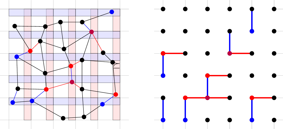
Since \(R_c^{\texttt{CN}}(p)\leq R_c^{\texttt{NN}}(p)\), we only have to prove the upper bound for \(R_{c}^{\texttt{NN}}(p)\). To this end, we use a coupling argument, and compare \(\Gamma_{p,R}^{\texttt{NN}}(P)\) with a Bernoulli percolation configuration \(G_B(P)\) associated to the same set \(P\) of points.
Let \(\varepsilon>0\), and let \(R=\|(1,1+\varepsilon)\|_p\). We define the set of edges \(E_B(P)\) of the (undirected) graph \(G_B(P) = (\mathbb{Z}^2,E_B(P))\) by, for \(i,j\in\mathbb{Z}\):
\(\big((i,j),(i+1,j)\big)\in E_B(P) \iff X_{i,j}>i+1-\varepsilon\),
\(\big((i,j),(i,j+1)\big)\in E_B(P) \iff Y_{i,j}>j+1-\varepsilon\),
see an example of construction in Figure 20.
We clearly have \(E_B(P)\subset E_{p,R}^{\texttt{NN}}(P)\). Hence, if \(G_B(P)\) percolates (i.e.has an infinite connected component), then \(\Gamma_{p,R}^{\texttt{NN}}(P)\) percolates.
Moreover, under the law \(\mathbb{P}\) on \(P\) defined in the Introduction, observe that each edge of the square lattice belongs to \(E_B(P)\) with probability \(\varepsilon\), independently of the other edges. Since the threshold for Bernoulli bond percolation on \(\mathbb{Z}^2\) is equal to \(1/2\), it follows that, for any \(R > \|(1,\frac{3}{2})\|_p\), \(\mathbb{P}(|\mathcal{C}_B(P)|=\infty)>0\).
4.1.0.2 Lower bound.
We again use a coupling argument. Let \(\Gamma_{R}^{\texttt{dec}}(P)= (\mathbb{Z}^2,E_{R}^{\texttt{dec}}(P))\) be the (undirected) subgraph of the square lattice whose set of edges \(E_{R}^{\texttt{dec}}(P)\) satisfies, for \(i,j\in\mathbb{Z}\):
\(\big((i,j),(i+1,j)\big)\in E_{R}^{\texttt{dec}}(P) \iff |X_{i,j} - X_{i+1,j}|\leq R\),
\(\big((i,j),(i,j+1)\big)\in E_{R}^{\texttt{dec}}(P) \iff |Y_{i,j} - Y_{i,j+1}|\leq R\).
We say that such a graph \(\Gamma_R^{\texttt{dec}}(P)\) is a configuration of the decorrelated model of parameter \(R\), and we denote by \(R_c^{\texttt{dec}}\) the critical radius of this new model. For any \(P\in\mathcal{P}\), we have \(E_{p,R}^{\texttt{NN}}(P)\subset E_R^{\texttt{dec}}(P)\). Thus, \(R_c^{\texttt{dec}}\leq R_c^{\texttt{NN}}(p).\) Therefore, it suffices to establish the lower bound \[\sqrt{2-\sqrt{2}}\leq R_c^{\texttt{dec}}.\]
To do that, we show that if \(R < \sqrt{2-\sqrt{2}}\), then the dual graph of \(\Gamma_R^{\texttt{dec}}(P)\) almost surely percolates. We denote this dual graph by \(\overline{\Gamma}_R^{\texttt{dec}}(P) = \left(\left(\frac{1}{2},\frac{1}{2}\right)+\mathbb{Z}^2,\overline{E}_R^{\texttt{dec}}(P)\right)\). Recall that, by definition, \(e\in E_R^{\texttt{dec}}(P) \iff \overline{e} \notin \overline{E}_R^{\texttt{dec}}(P)\), where for an edge \(e\) of the standard square lattice, we denote by \(\overline{e}\) the corresponding (orthogonal) edge in the dual lattice.
Let us consider the set \(E'\) of edges of the dual square lattice obtained by conserving only the edges of one line over two, and of one column over two, see Figure 21. Mathematically, it is defined by: \[\begin{align} E'= & \left\{\left((1/2+2i,1/2+j),(1/2+2i,3/2+j)\right) : i,j \in \mathbb{Z}\right\} \\ & \quad \cup \left\{\left((1/2+i,1/2+2j),(3/2+i,1/2+2j)\right) : i,j \in \mathbb{Z}\right\}. \end{align}\]
We claim that each edge of \(E'\) belongs to \(\overline{E}_R^{\texttt{dec}}(P)\) with probability \[1-p_R = 1-\mathbb{P}\left(\left((0,0),(1,0)\right)\in E_R^{dec}(P)\right)=1-\mathbb{P}\left(|X_{0,0} - X_{1,0}|\leq R\right),\] independently of the other edges of \(E'\).
Indeed, the horizontal edge \(((1/2+2i,1/2+j),(1/2+2i,3/2+j)) \in E'\) belongs to \(\overline{E}_R^{\texttt{dec}}(P)\) if and only if \(|Y_{2i,j} - Y_{2i,j+1}| > R\). This happens with probability \(1-p_R\), and furthermore, two distinct horizontal edges depend on different random variables. So, all horizontal edges are independent. Similarly, all vertical edges are independent. And, since horizontal edges depend on \(Y\) random variables, and vertical edges on \(X\) random variables, all edges are independent.
By grouping consecutive edges of \(E'\) in pairs, and comparing with Bernoulli bond percolation on the square lattice of parameter \((1-p_R)^2\), we obtain that if \((1-p_R)^2>1/2\), then the restriction of \(\overline{\Gamma}_R^{\texttt{dec}}(P)\) to the edges of \(E'\) has almost surely an infinite connected component, so that \(\overline{\Gamma}_R^{\texttt{dec}}(P)\) percolates almost surely. Furthermore, standard results on Bernoulli percolation imply that in this case, every vertex of \(\mathbb{Z}^2\) is almost surely surrounded by the infinite connected component, so that \(\Gamma_R^{\texttt{dec}}(P)\) has almost surely no infinite connected component. For \(R\leq1\), we have \(p_R=\frac{R^2}{2}\). As a consequence, if \(R<\sqrt{2-\sqrt{2}}\), then \(\Gamma_R^{\texttt{dec}}(P)\) has almost surely no infinite connected component. It follows that \(R_c^{\texttt{dec}}\geq \sqrt{2-\sqrt{2}}\).
4.2 Estimates↩︎
In Figure 22, we provide estimates of the critical radius for some values of the parameter \(p\), both for the complete neighbor model and for the nearest neighbor one.

To obtain these values, we estimated the probability for the origin to be connected to a border of the grid \([-N,N]^2\), for \(N=40\). Precisely, for each \(R=0.005\times n\) with \(n\geq 0\), we ran \(1000\) simulations of the models on the grid \([-40,40]^2\). The approximations of \(R_c\) given in the table then correspond to the first integers \(n\geq 0\) such that for at least one of the \(1000\) simulations, the origin was connected to a border of the grid.
In Figure 2 and 3, our estimates of the critical are represented with crosses.
5 Perspectives↩︎
5.0.0.1 Critical radius.
Theorem 6 provides lower and upper bounds of the critical radius, for both the complete neighbor and the nearest neighbor model. However, the exact values remain to be determined. In Section 4.2, we propose numerical estimations of the critical radius, obtained with the help of computer simulations. They suggest that for the nearest neighbor model with \(p=\infty\), the critical radius is equal to \(1\). For \(p=\infty\) and \(R\geq 1\), \(\Gamma_{\infty,1}^{\texttt{NN}}(P)\) coincides with the decorrelated model \(\Gamma_1^{\texttt{dec}}(P)\) introduced in Section 4. We thus state the following conjecture.
Conjecture 7. \(R_c^{\texttt{NN}}(\infty) = R_c^{\texttt{dec}} = 1\).
This conjecture is supported by the following properties.
For \(R=1\), the density of edges is equal to: \[{\mathbb{P}}(((0,0),(0,1))\in E_{\infty,1}^{\texttt{NN}}(P))={\mathbb{P}}(X_{1,0}-X_{0,0}\leq 1)=1/2,\] a value that coincides with the critical probability for Bernoulli percolation on the square lattice. Moreover, the states of any two edges are independent, unless they constitute consecutive edges on a same horizontal or vertical line. Observe also that the probability of any finite pattern has a rational value, that can be computed in terms of counting permutations.
The decorrelated model exhibits a remarkable symmetry property with respect to the value \(R=1\). Precisely, for \(R\in[0,2]\), let us denote by \(\widetilde{\Gamma}_{R}^{\texttt{dec}}(P)\) the subgraph of the lattice obtained from \(\Gamma_{R}^{dec}(P)\) by switching the open and closed edges. Then, \(\widetilde{\Gamma}_R^{\texttt{dec}}(P)\) and \(\Gamma_{2-R}^{\texttt{dec}}(P)\) have the same distribution.
5.0.0.2 Unicity of the infinite connected component.
In the super-critical regime, we conjecture that there is almost surely a unique infinite connected components, both for the complete model and for the nearest neighbor one. It seems that the proof strategy developed by Burton and Keane BK89? for Bernoulli percolation can be used to prove the uniqueness for the nearest neighbor model with \(p=\infty\) (at least), but what about the general case?
5.0.0.3 Asymptotic shape of the connected component of the origin.
For a graph \(G=(\mathbb{Z}^2, E)\), let us denote by \({\mathcal{B}}_n(G)\) the set of points of \(\mathbb{Z}^2\) that are at distance smaller than \(n\) from the origin \((0,0)\) for the graph distance in \(G\), that is: \[{\mathcal{B}}_n(G)=\{v\in \mathbb{Z}^2 : \exists u_0=(0,0),u_1,\ldots, u_{n-1},u_n=v \in \mathbb{Z}^2, \forall i\in\{0,\ldots, n-1\}, (u_i,u_{i+1})\in E\}.\]
We expect the diameter of \({\mathcal{B}}_n(\Gamma_{p,R}^{\texttt{CN}}(P))\) to grow linearly, at least for \(R\geq R^{\texttt{CN}}_{max} (p)\). What can we say about the asymptotic shape of the set \[\frac{1}{n}\Big({\mathcal{B}}_n(\Gamma_{p,R}^{\texttt{CN}}(P))+[0,1]^2\Big)\] when \(n\) tends to the infinity? When \(R\) goes to infinity, does this shape become close to the ball of the corresponding \({\mathcal{L}}_p\)-norm? And what about the counterpart of this shape for the nearest neighbor model?
5.0.0.4 Gilbert’s disc model conditioned on other lattices.
In this article, we focused on Gilbert’s disc model conditioned on the square lattice. The definitions naturally extend to other lattices (triangular or hexagonal lattice, \(d\)-dimensional lattices...). What are then the values of the possible connectivity radius, of the critical radius, and of the total connectivity radius?
6 Appendix↩︎
6.1 Proof of Lemma 5↩︎
Let \(u\) be a path of \(\Gamma_{p,R}^{\texttt{NN}}(P)\). Firstly, the pattern observed between the points \(u_0\) and \(u_4\) is one of the patterns observed for the case \(a_{k+1}-a_k=3\) at the end of section 3.3.3. So by similar arguments used for Equation 4 , we have \[\label{eq:Y9540244141} Y_{2,1} \leq 1+ \left[(2R)^p - \left(1 - (X_{1,0}-1) \right)^p\right]^{\frac{1}{p}}.\tag{8}\]
Since \(Y_{1,3}\leq Y_{2,1} + 3R\), we have \[\label{eq:R60R40p41L1461} (Y_{1,3} - 3) - (X_{1,0} - 1) \leq \big[(2R)^p - \left(1 - (X_{1,0}-1) \right)^p\big]^{\frac{1}{p}} + 3R - 2 - (X_{1,0}-1).\tag{9}\]
6.1.0.1 Case \(p\leq \displaystyle\frac{\ln(2)}{\ln(\frac{4}{3})}\).
By Lemma 1, \(\min\{1/2,R(p)\} = 1/2\). Using the inequality \(R<1/2\), we obtain \[\label{eq:R60R40p41L1462} \big[(2R)^p - \left(1 - (X_{1,0}-1) \right)^p\big]^{\frac{1}{p}} + 3R - 2 - (X_{1,0}-1) < \big[1 - \left(1 - (X_{1,0}-1) \right)^p\big]^{\frac{1}{p}} - \frac{1}{2} - (X_{1,0}-1).\tag{10}\] To conclude, we show that for all \(x\in[0,R]\), the following inequality holds: \[1 \leq (1-x)^p + \left(\frac{1}{2}+x \right)^p.\] To this purpose, we set the function \(g(x)=(1-x)^p + \left(\frac{1}{2}+x\right)^p\), for \(x\in[0,R]\).
By studying its derivative, we obtain that \(g\) admits a minimum in \(x= 1/4\). Thus, for all \(x\in[0,R]\), \[g(x)\geq g\left(\frac{1}{4}\right) = 2\left(\frac{3}{4}\right)^p\geq 2\left(\frac{3}{4}\right)^{\frac{\ln(2)}{\ln(\frac{4}{3})}}=1.\]
As a consequence, taking \(x = X_{1,0}-1\), we obtain that, for any \(x\in[0,R]\), \[\big[1 - \left(1 - (X_{1,0}-1) \right)^p\big]^{\frac{1}{p}} - \frac{1}{2} - (X_{1,0}-1) \leq 0.\] And, by Equation 10 and since \([1,1+R]\) is compact, there exists \(c_1 > 0\), \[\big[\big(2R\big)^p - (1-(X_{1,0}-1))^p\big]^{\frac{1}{p}} +3R -2 -(X_{1,0}-1) \leq -c_1<0,\] and so, by Equation 9 , \((Y_{1,3} - 3) - (X_{1,0} - 1) \leq -c_1 < 0.\)
6.1.0.2 Case \(p> \displaystyle\frac{\ln(2)}{\ln(\frac{4}{3})}\).
By Lemma 1, \(\min\{1/2,R(p)\} = R(p)\), hence \(R< R(p)\), and so \[\begin{align} & \big[(2R)^p - \left(1 - (X_{1,0}-1) \right)^p\big]^{\frac{1}{p}} + 3R - 2 - (X_{1,0}-1) \nonumber\\ &\quad < \big[(2R(p))^p - \left(1 - (X_{1,0}-1) \right)^p\big]^{\frac{1}{p}} + 3R(p) - 2 - (X_{1,0}-1) \label{eq:R60R40p41L1463} . \end{align}\tag{11}\] To conclude, we show that for all \(x\in[0,R]\), the following inequality holds: \[(2R(p))^p \leq (1-x)^p + (2+x-3R(p))^p.\] To this purpose, we set the function \(g(x)=(1-x)^p+(2+x-3R(p))^p\), for \(x\in[0,R]\).
By studying its derivative, we obtain that \(g\) admits a minimum in \((3R(p)-1)/2\). Thus, for all \(x\in[0,R]\), \[g(x)\geq g\left(\frac{3R(p)-1}{2}\right) = 2\left(\frac{3-3R(p)}{2}\right)^p.\] As \(R(p) < 1/2\) and by its definition, see Lemma 1, \[2\left(\frac{3-3R(p)}{2}\right)^p\geq \bigg(\frac{3-3R(p)}{2}\bigg)^p + \bigg(\frac{2-R(p)}{2}\bigg)^p=(2R(p))^p.\]
As a consequence, taking \(x = X_{1,0}-1\), we obtain that, for any \(x\in[0,R]\), \[\big[\big(2R(p)\big)^p - (1-(X_{1,0}-1))^p\big]^{\frac{1}{p}} +3R(p) -2 -(X_{1,0}-1) \leq0.\] And, by Equation 11 and since \([1,1+R]\) is compact, there exists \(c_1 > 0\), \[\big[\big(2R\big)^p - (1-(X_{1,0}-1))^p\big]^{\frac{1}{p}} +3R -2 -(X_{1,0}-1) \leq -c_1<0,\] and so, by Equation 9 , \((Y_{1,3} - 3) - (X_{1,0} - 1) \leq -c_1 < 0.\)
6.2 Proof of Lemma 6↩︎
Let \(u\) be a path of \(\Gamma_{p,R}^{\texttt{NN}}(P)\). Then we have \[\|P_{1,3}-P_{2,2}\|_p^p = (X_{1,3}-X_{2,2})^p + (Y_{1,3}-Y_{2,2})^p \leq (2R)^p.\]
Using \(Y_{1,3}\in[3,4]\) and \(X_{2,2}\in[2,3]\), we obtain \[(2-X_{1,3})^p +(3-Y_{2,2})^p\leq (2R)^p.\]
Since \(Y_{2,2} < Y_{2,1} + R(p)\) and by Equation 8 , it follows that \[\begin{align} X_{1,3}&\geq 2 - \big((2R)^p-(3-Y_{2,2}))^p\big)^{\frac{1}{p}}\\ &\geq 2 - \bigg[(2R)^p-\bigg(2-R-\big[(2R)^p-(1-(X_{1,0}-1))^p\big]^{\frac{1}{p}}\bigg)^p\bigg]^{\frac{1}{p}}. \end{align}\] Since \(X_{-1,2} \geq X_{1,3} - 3\), it implies that \[\begin{align} (1 + (-1) - X_{-1,2}) - (X_{1,0}-1) &\leq 3R- X_{1,3} - (X_{1,0}-1)\\ & \leq \left[(2R)^p-\left(2-R-\left[(2R)^p-(1-(X_{1,0}-1))^p\right]^{\frac{1}{p}}\right)^p\right]^{\frac{1}{p}}\nonumber \\ &+ 3R - 2 - (X_{1,0}-1)\tag{12} \\ & < \left[(2R(p))^p-\left(2-R(p)-\left[(2R(p))^p-(1-(X_{1,0}-1))^p\right]^{\frac{1}{p}}\right)^p\right]^{\frac{1}{p}} \nonumber \\ &+ 3R(p) - 2 - (X_{1,0}-1)\tag{13} \end{align}\]
To conclude, we show that for all \(x\in[0,R]\), the following inequality hold: \[[(2R(p))^p - (2+x-3R(p))^p]^{\frac{1}{p}} + [(2R(p))^p - (1-x)^p]^{\frac{1}{p}}< 2-R(p).\]
To this purpose, we set the function \[g(x) = [(2R(p))^p - (1 - x)^p]^{\frac{1}{p}} + [(2R(p))^p - (2 + x - 3R(p))^p]^{\frac{1}{p}} ,\] for \(x\in[0,R]\). By studying its derivative, we obtain that \(g\) admits a maximum in \((3R(p)-1)/2\). Thus, for all \(x\in[0,R]\), \[g(x)\leq g\left(\frac{3R(p)-1}{2}\right) = 2\left[(2R(p))^p - \left(\frac{3-3R(p)}{2}\right)^p\right]^{\frac{1}{p}}.\]
By Equation ?? , we obtain \[g\left(\frac{3R(p)-1}{2}\right) = 2-R(p).\]
As a consequence, taking \(x=X_{1,0}-1\), we obtain that, for any \(X_{1,0}\in[1,1+R]\), \[\bigg[(2R(p))^p-\bigg(2-R(p)-\big[(2R(p))^p-(1-(X_{1,0}-1))^p\big]^{\frac{1}{p}}\bigg)^p\bigg]^{\frac{1}{p}}+ 3R(p) - 2 - (X_{1,0}-1)\leq 0.\] And, by Equation 13 and since \([1,1+R]\) is compact, there exists \(c_2 > 0\) such that \[\bigg[(2R)^p-\bigg(2-R-\big[(2R)^p-(1-(X_{1,0}-1))^p\big]^{\frac{1}{p}}\bigg)^p\bigg]^{\frac{1}{p}}+ 3R - 2 - (X_{1,0}-1)\leq -c_2,\] and so, by Equation 12 , \((1 + (-1) - X_{-1,2}) - (X_{1,0} - 1) \leq -c_2\).