Transforming Rank: How Architecture Navigates the Spectral Pathologies of Depth
July 15, 2026
Abstract
We investigate how each component of the Transformer feedforward block architecture design determines how much rank survives across depth at initialization. We reinterpret skip connections and normalization, long understood as controlling magnitude, as mechanisms for preserving gradient rank across depth, since the very matrix multiplications and nonlinear activations that make the network expressive also reduce the rank. We show that skip connections trade off rank collapse against ensemble-like behavior, controlled by the relative scales of the branch and the skip: skip connections route the gradient around the residual branch, where rank is lost, rather than along the long gradient paths that encourage the layers to compose. The placement of the normalization layer controls this same tradeoff by setting the branch-to-skip ratio across depth, unifying much of the normalization placement and depth scaling literature, in particular why rank collapses for Post-Norm but plateaus for Pre-Norm. Other aspects of the architecture, like the two-matrix structure that expands and contracts the width, use additional parameters to preserve the representation or branch Jacobian rank. The second matrix decorrelates a coherent mean spike that would grow across blocks with a single matrix and uncentered activation, preventing the residual representation from collapsing. The width expansion between the two matrices keeps the branch Jacobian full rank: applying the rank-reducing activation in this expanded space leaves enough directions to span the original, at a width that follows a Marchenko–Pastur law. The initialization rank of the input–output Jacobian predicts which networks train on CIFAR-10. Taken together, we recast architecture design for deep networks as navigating an intrinsic tradeoff among rank collapse, ensemble-like behavior, and parameter count. Code is available at https://github.com/everettk/transforming-rank-paper.
1 Introduction↩︎
The modern Transformer feedforward block has a specific structure: each block normalizes the residual stream, expands the hidden dimension by a factor of roughly four through a pair of up- and down-projection matrices, applies an elementwise activation between them, and adds the result back to the residual stream, \[h_\ell = h_{\ell-1} + W_{\mathrm{down}}\,\sigma\!\left(W_{\mathrm{up}}\,\mathrm{Norm}(h_{\ell-1})\right).\]
The overall structure of this feedforward block is almost exactly what the original Transformer paper [1] proposed nearly a decade ago: what has changed in practice is the placement of the normalization layer, from Post-Norm to Pre-Norm [2], [3], and the choice of activation, from ReLU through GELU [4] to gated units [5]. Outside the feedforward block, there have been Transformer architecture innovations adopted widely in practice, including mixture-of-expert models [6], [7] and modifications of attention [8], [9]. However, the design of the feedforward block itself has been exceptionally stable over time even as frontier models have scaled up to hundreds of billions or more parameters.
Even at these scales, the depth of frontier models remains on the order of a hundred layers [10], [11]. Training deep Transformers has challenges with training stability [12], [13], diminishing returns from additional layers [14]–[16], and signal propagation across depth [17]. One form of signal degradation is rank collapse: the rank of the gradients and representations decreases through the layers, until they span only a small number of directions in a high-dimensional space [18]. In this work, we investigate how the architecture of the feedforward block determines the effective rank of the gradients and representations in deep networks.
In a plain MLP, the input–output Jacobian, the gradient of the network output with respect to its input, is a product of matrices: each layer contributes a weight matrix and a diagonal matrix of activation derivatives. Since a product of matrices can only lose rank with each additional matrix multiplication, the Jacobian rank decreases monotonically with depth. The literature on dynamical isometry shows that the only way to avoid this rank loss in a plain MLP is for every per-layer Jacobian to have all singular values near one [19], [20]: this requires that neither the weight matrices nor the activation derivatives reduce rank. In particular, the activation function trades off expressivity against rank: an activation that preserves rank must have a derivative near one in magnitude [20]; therefore, a nonlinearity that makes the network expressive also reduces the Jacobian rank [21]. Outside of dynamical isometry, where typical neural networks operate, every layer of a plain MLP is a rank-reducing operation for the Jacobian.
Skip connections [22] and normalization layers [23], [24] are usually thought of as ways to keep the gradient and representation magnitudes from vanishing or exploding with depth, whereas we reinterpret them as mechanisms for bypassing rank loss in the gradient. We show that skip connections preserve rank by routing the gradient around the residual branch, where rank is lost, then restoring the rank through the identity path around the branch that is trivially full-rank. The branch scale and initialization control how much of the gradient flows through the residual branch versus around it, which comes with a tradeoff: at the extreme, if all the gradient flowed around the branch, the network would act like an ensemble of individual layers rather than a deep network whose layers compose. We further show that the placement of the normalization layers controls this same ratio between the branch and skip, and therefore the tradeoff between rank collapse and ensemble regimes; this perspective unifies many recent results on normalization placement and depth scaling.
On the other hand, we show that the two-matrix structure in each feedforward block actually preserves the rank of the residual branch Jacobian. The branch expands the hidden dimension with its first matrix, applies the activation, and contracts back with the second matrix. Although the activation still reduces rank, applying it in this expanded space rather than the model dimension lets enough directions survive to keep the branch Jacobian full rank. In addition, the second matrix decorrelates the residual branch means, so the representation does not collapse onto a single direction.
We argue there is a logical chain of architectural choices that navigate the rank tradeoff across depth, building up from a plain MLP to the modern feedforward block. We measure the effective rank at initialization of the input–output Jacobian, the residual stream representation, and the residual branch Jacobian, and show that the rank of the input–output Jacobian predicts which networks train on CIFAR-10. Our contributions are as follows:
We show that skip connections preserve rank by routing the gradient around the rank-reducing branch through the full-rank identity path, creating a tradeoff between rank collapse and ensemble-like behavior, controlled by the relative magnitudes of the branch and skip paths (Section 3).
We show that the normalization placement determines the rank by controlling this same branch-to-skip ratio across depth: Post-Norm holds it constant and the rank collapses, while Pre-Norm lets it decay so the rank plateaus at a moderate level, at the expense of its deep layers shifting back toward the ensemble regime. The projection terms in the normalization operation contribute negligible rank loss compared to the branch-to-skip ratio. This same ratio controls a \(\sqrt{L}\) depth factor in the initialization rank and unifies a range of results on normalization placement and depth scaling (Section 4).
We show the two-matrix structure in the feedforward block preserves residual representation rank. With a single matrix and an uncentered activation, the rank of the residual representation collapses through a coherent mean spike whose cross-layer alignment equals the activation moment ratio \(c_\ell = \mathbb{E}[\sigma]^2/\mathbb{E}[\sigma^2]\). The second matrix decorrelates this alignment to zero and prevents the collapse (Section 5).
We show the width expansion between the two matrices preserves rank in the branch Jacobian. The activation function reduces the rank by masking or attenuating directions; applying this operation in the expanded space means enough directions survive to span the original space. We derive from a Marchenko–Pastur law the threshold \(m/d = 1/p(\sigma)\) at which the branch Jacobian becomes full rank, where \(p\) is the survival rate of the activation (\(1/2\) for ReLU; \(p = \mathbb{E}[\sigma'(z)^2]\) for smooth activations; Section 6).
In this work, we focus primarily on the initialization rank across depth in a network of feedforward blocks. Related work studies the rank collapse that occurs in attention layers [17], [25] and how rank evolves throughout training [26], [27]. Even at initialization, the rank behavior across depth illustrates how the components of the feedforward block, though usually understood in other terms, together navigate an intrinsic tradeoff among rank collapse, ensemble-like behavior, and parameter count: skip connections and normalization route the gradient around the rank-reducing branch, trading off rank collapse against ensemble-like behavior, while the two-matrix structure and width expansion preserve the branch and representation rank at the cost of additional parameters.
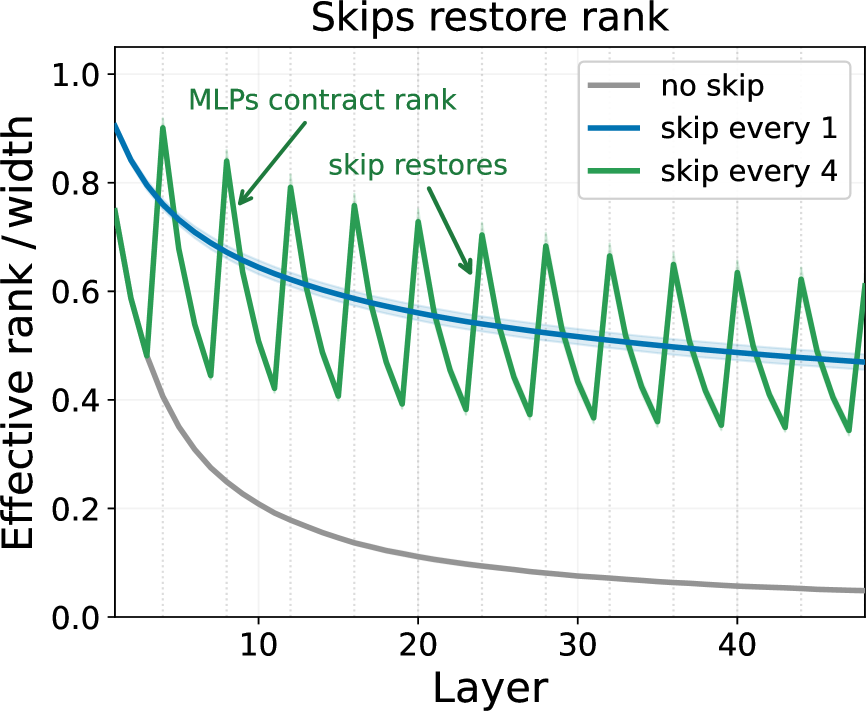
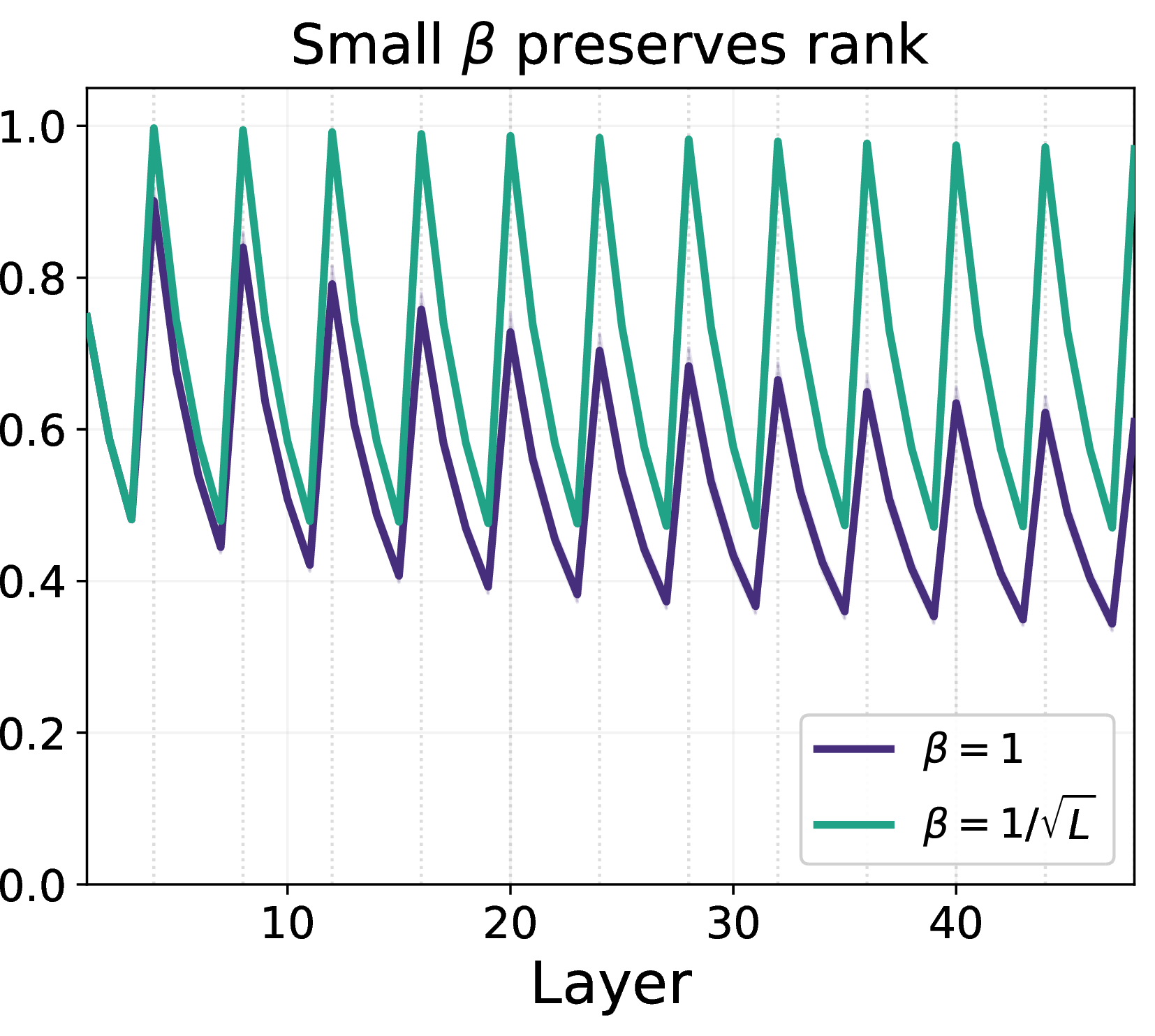
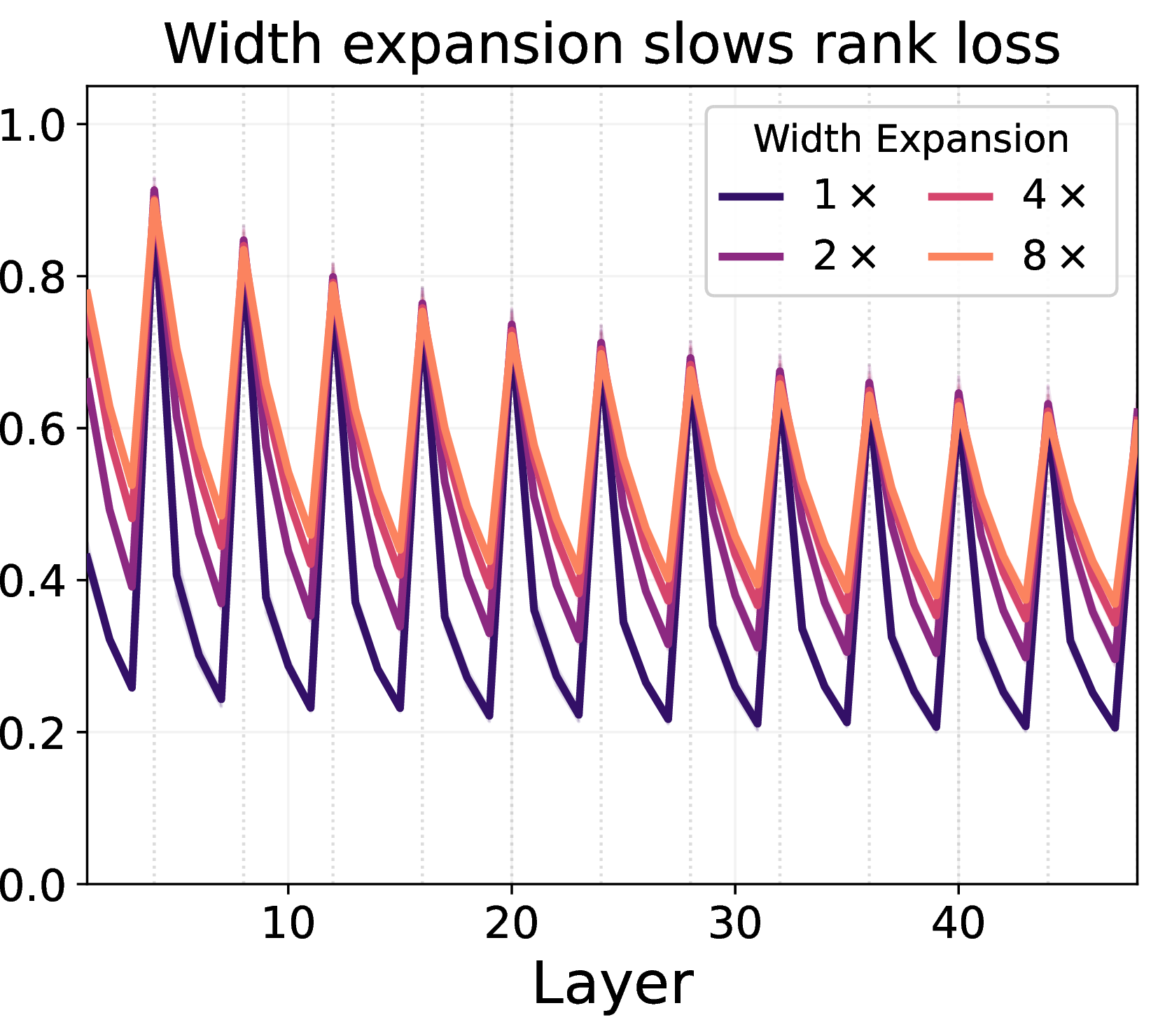
Figure 1: Skip connections restore the effective rank that each feedforward block contracts; the residual scale \(\beta\) and the width expansion control how much survives with depth. Effective rank of the Jacobian \(\partial h_\ell / \partial h_0\) up to each layer \(\ell\), normalized by the width (model dimension) \(d\), for a Pre-Norm ReLU residual MLP (\(L = 48\), \(d = 256\), \(\beta = 1\), \(\alpha = 1\), and \(4\times\) width expansion unless otherwise stated; mean over 12 seeds). Left: rank collapses without skips (gray); rank decays smoothly with a skip on every block (blue); spacing skips to every fourth block reveals the mechanism (green): rank contracts through the feedforward blocks and is restored at each skip. Center: scaling the residual branch by \(\beta = 1/\sqrt{L}\) reduces the magnitude of its contribution relative to the skip; since the skip (identity function) dominates, rank is preserved across depth, unlike at \(\beta = 1\). Right: residual branches with higher width expansion factors lose rank more slowly, raising the sawtooth troughs, a per-block conditioning effect analyzed in Section 6..
2 Setup↩︎
We consider a residual network in which an input \(h_0 \in \mathbb{R}^d\) is transformed by \(L\) residual blocks into \(h_L\). Each residual block has the form \[h_\ell = h_{\ell-1} + \beta\, f(h_{\ell-1}), \qquad \ell = 1, \dots, L, \label{eq:residual-block}\tag{1}\] with branch scale \(\beta\). The branch \(f\) may itself include a normalization, an elementwise activation \(\sigma\), and one or two weight matrices; we write \(M\) for the number of branch matrices. By default the branch is the two-matrix feedforward block, \(f(h) = W_{\mathrm{down}}\,\sigma(W_{\mathrm{up}}\,\mathrm{Norm}(h))\), with \(W_{\mathrm{up}} \in \mathbb{R}^{m \times d}\) and \(W_{\mathrm{down}} \in \mathbb{R}^{d \times m}\), where \(m/d\) is the expansion ratio. Unless stated otherwise, the activation is ReLU, the normalization is RMSNorm in the Pre-Norm placement, \(\beta{=}1\), and the weights are initialized as \(\mathcal{N}(0, \alpha^2/\text{fan-in})\) with initialization scale \(\alpha = 1\).
We track the rank, across depth, of three objects. The first is the input–output Jacobian \(\partial h_L/\partial h_0\), an ordered product over the \(L\) blocks, \[\frac{\partial h_L}{\partial h_0} = (I + \beta J_L)(I + \beta J_{L-1})\cdots(I + \beta J_1), \label{eq:io-jacobian}\tag{2}\] where \(J_\ell := \partial f(h_{\ell-1})/\partial h_{\ell-1}\) is the branch Jacobian of block \(\ell\). The other two are the forward residual representation \(Z_\ell\) (Section 5) and the branch Jacobian on its own, whose normalization-free core is written \(J_f\) (Section 6).
We report two spectral measures of a matrix \(A\) with \(N\) singular values \(\sigma_1 \ge \cdots \ge \sigma_N\). Our primary measure is the effective rank [28], the exponential of the spectral entropy, \[\operatorname{erank}(A) = \exp\!\Bigl(-\textstyle\sum_k p_k \ln p_k\Bigr), \qquad p_k = \sigma_k\big/\textstyle\sum_j \sigma_j, \label{eq:erank}\tag{3}\] which we report normalized by the model dimension \(d\) as \(\operatorname{erank}(\partial h_L/\partial h_0)/d\); it equals \(1\) when all singular values are equal and drops toward \(0\) as the spectrum collapses in a few directions. We also use the stable rank \(\operatorname{st}(A) = \lVert A\rVert_F^2/\lVert A\rVert_2^2\), primarily in Section 5. Both measures are scale-invariant and lie in \([1, N]\). For Jacobian measurements taken at initialization, we sample a random Gaussian input and evaluate each branch Jacobian at the resulting forward activations, reporting means over independent samples of the weights and the input unless stated otherwise.
3 Skip Connections and Rank Restoration↩︎
A plain MLP loses effective rank with depth due to repeated matrix multiplications and nonlinearities: its per-layer Jacobians are each mildly deficient in effective rank, and composing them compounds the loss across depth. The only exception is networks satisfying the dynamical isometry condition, which requires every singular value of the input–output Jacobian to remain close to one, so that effective rank is preserved at any depth [19]. However, dynamical isometry in neural networks is difficult to achieve in practice, requiring orthogonal initialization and precise choices of activation function and activation distribution maintained throughout training [20], [21].
Skip connections are often understood as an architectural solution to vanishing gradient magnitude across depth; we reinterpret them as a solution to vanishing gradient rank across depth. Gradients that flow through many MLP layers inevitably lose rank, because the matrix multiplications and nonlinearities that make the network expressive also reduce rank. Skip connections, in that sense, are a workaround to this intrinsic rank loss: they preserve rank because they route the gradient around the residual branch, where rank is lost, through an identity path that is trivially full rank. This creates a sawtooth pattern in the rank across depth if the skips are spaced across multiple layers, where rank decreases through the MLPs and is restored at each skip connection (Figure 1, left). In this section, we argue that the deep residual architecture navigates a fundamental tradeoff: if all of the gradient passed through the branch, the rank would collapse; if it all passed through the skips, the network would act like an ensemble of individual layers rather than a deep network whose layers compose.
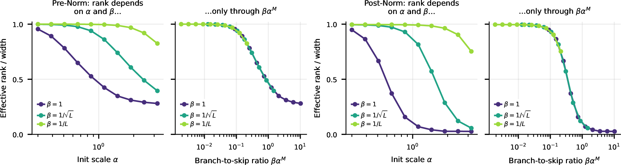
The standard residual block contains a scaled branch added to an identity skip connection, \(h_\ell = h_{\ell-1} + \beta f(h_{\ell-1})\). When the residual stream passes through each block untouched, as it does under Pre-Norm (Appendix 11), the skip term must be the identity: scaling it by \(\lambda\) multiplies its contribution by \(\lambda^{L-\ell}\), which explodes for \(\lambda > 1\) and vanishes for \(\lambda < 1\) [29]. The branch has two parameters that control its scale, the branch scale \(\beta\) and the initialization scale \(\alpha\) of its weight matrices. The Jacobian of a single block contains a skip term and a branch term; we define the branch-to-skip ratio \(r_\ell\) for each layer as the ratio of their Frobenius norms: \[\frac{\partial h_\ell}{\partial h_{\ell-1}} = \underbrace{I}_{\text{skip}} + \underbrace{\beta J_\ell}_{\text{branch}}, \qquad r_\ell \equiv \frac{\|\beta J_\ell\|_F}{\|I\|_F}. \label{eq:branch-skip}\tag{4}\] At unit residual stream scale, \(r_\ell = \sqrt{p}\,\beta\alpha^{M}\): the branch Jacobian contributes one factor of \(\alpha\) for each of the \(M\) weight matrices, and a factor \(\sqrt{p}\) from the activation derivative, where \(p = \mathbb{E}[\sigma'(z)^2]\) (\(p = 1/2\) for ReLU; for activations whose derivative is zero or \(\pm 1\), this is the survival rate in Section 6). We will analyze the depth dependence of \(r_\ell\) in Section 4. For residual networks with positively homogeneous activations, there are equivalence classes over the initialization scale \(\alpha\) and the branch scale \(\beta\) in which networks with the same value of \(\beta\alpha^{M}\) compute the same function at initialization. This equivalence persists throughout training if the optimizer hyperparameters are rescaled accordingly for each matrix (Appendix 11.4). In particular, we show that the effective rank at initialization depends on \(\beta\) and \(\alpha\) only through \(\beta\alpha^{M}\), for both Pre- and Post-Norm (Figure 2). A larger \(\beta\alpha^{M}\) sends more of the gradient through the branch rather than the skip, so the rank collapses faster with depth.
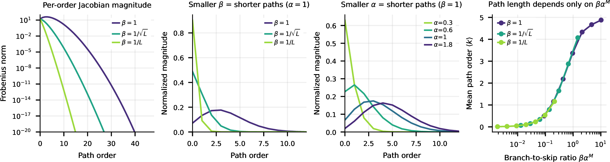
Prior work shows that deep residual networks behave like ensembles of shallow networks [15], [30]. [30] decompose a residual network forward pass into \(2^L\) paths that take either the skip or the branch at each block. We apply a similar expansion to the input–output Jacobian, where the skip contributes the identity and the branch contributes \(\beta J_\ell\) to the product. Grouping the paths by their order \(k\), the number of blocks at which a path takes the branch rather than the skip, gives \[\frac{\partial h_L}{\partial h_0} = \sum_{k=0}^{L} \beta^k S_k, \qquad S_k = \sum_{1 \le \ell_1 < \cdots < \ell_k \le L} J_{\ell_k} \cdots J_{\ell_1}, \label{eq:path-decomp}\tag{5}\] where each order-\(k\) path carries weight \((\beta\alpha^{M})^k\). We say a path is short if it passes through few feedforward blocks (small \(k\)) and runs mostly through the skip connections; a long path (large \(k\)) passes through many feedforward blocks. Because the path weight is raised to the order \(k\), small changes in \(\beta\) and \(\alpha\) are amplified in the long paths. Small changes in the ratio therefore induce significant shifts in the distribution over path orders (Figure 3): at a small ratio the short paths dominate, which encourages the network to behave like an ensemble of shallow subnetworks more than a deep network whose layers compose. This same ratio also controls whether the rank shows a flat or a decaying sawtooth pattern: at \(\beta = 1/\sqrt{L}\) each skip nearly restores the rank lost in the preceding block, whereas at \(\beta = 1\) it restores only part and rank declines with depth (Figure 1, center).
Our decomposition lets us reinterpret the downscaling of the residual branch, often recommended in the depth-scaling literature, as a way to bypass rank collapse but possibly at the expense of composition. Multiple theoretical perspectives all propose \(\beta=1/\sqrt{L}\) scaling, motivated by gradient stability and an expressive infinite-depth kernel [31], feature learning and hyperparameter transfer [32], [33], and preventing rank collapse across the sequence dimension [17]. [34] show that residual networks with any activation function achieve dynamical isometry when the branch is downscaled sufficiently. In practice, though, many frontier models keep \(\beta=1\) [10], [11], [35]–[38] or similarly rescale the skip connection [39], suggesting the stronger branch contribution may bring empirical benefits on downstream tasks that downscaling would sacrifice.
A network that does not downscale the branch needs normalization layers to control the growing magnitude of the residual stream; as the next section will show, the normalization placement also determines how the branch-to-skip ratio, and therefore the rank, evolves with depth. At \(\beta=1\) the stream grows because the branch contributions accumulate rather than cancel at initialization (Appendix 11). Some methods avoid normalization entirely by initializing the branch near zero [12], [13], [40]: a small ratio limits the magnitude growth that normalization would otherwise control, at the same possible cost in composition as downscaling the residual branch with small \(\beta\).
4 Normalization Placement and the Branch-to-Skip Ratio↩︎
A normalization layer can be placed at three locations in a residual block: the branch input (Pre-Norm), the branch output (which we call Output-Norm), or the stream after the residual addition (Post-Norm) [41]. The original Transformer used Post-Norm [1], \[h_\ell = \mathrm{Norm}\bigl(h_{\ell-1} + \beta\, f(h_{\ell-1})\bigr), \label{eq:postnorm}\tag{6}\] but the canonical architecture today uses Pre-Norm [10], [11]: \[h_\ell = h_{\ell-1} + \beta\, f(\mathrm{Norm}(h_{\ell-1})). \label{eq:prenorm}\tag{7}\] The optimal placement of normalization layers is still debated, with recent work proposing that Post-Norm can be viable in deep networks [42]–[44] or that normalization is beneficial at other locations, including several per block or different placements at different depths [35], [41], [45]–[49].
We consider normalization operations at each location that subtract the mean, rescale the root-mean-square of the input, or do both.1 This section shows that the normalization placement and operation determine the effective rank through how the branch-to-skip ratio (Eq. 4 ) changes across depth: a post-residual rescaling holds the ratio constant and the rank collapses, whereas every other choice lets the ratio decay and the rank plateaus, provided a normalization fixes the scale of the branch. The rank measurements in this section use a single sample of the weights and the input, and the operations we compare share the same sample; each cell of the CIFAR heatmaps (Figure 6) trains one network per learning rate.
We first rule out a potential explanation for why the normalization placement affects the rank: prior work observes the normalization Jacobian contains a projection term that removes directions from the gradient [51], [52]. Deep Post-Norm networks show collapsed input–output Jacobian spectra already at initialization [12]. The mean subtraction operation removes the all-ones direction \(\mathbf{1}\), and the rescaling operation removes the current stream direction \(\hat{x} = h/\|h\|\) (with the normalization gain at its standard initialization of one): \[\frac{\partial}{\partial h}\bigl(h - \mu(h)\mathbf{1}\bigr) = \underbrace{I - \tfrac{1}{d}\mathbf{1}\mathbf{1}^{\top}}_{\text{removes } \mathbf{1}}, \qquad\quad \frac{\partial}{\partial h}\,\frac{h}{\mathrm{RMS}(h)} = \frac{\sqrt{d}}{\|h\|}\, \underbrace{\bigl(I - \hat{x}\hat{x}^{\top}\bigr)}_{\text{removes } \hat{x}}. \label{eq:norm-proj}\tag{8}\] The placement changes where the projection occurs relative to the identity. In the Post-Norm block Jacobian, \(J_{\mathrm{Norm}}(I + \beta J_f)\), every gradient path passes through the projection; in the Pre-Norm block Jacobian, \(I + \beta J_f J_{\mathrm{Norm}}\), the identity carries the gradient around it [52]. If the projection removes directions from the gradient, and the identity bypass protects the rank in Pre-Norm, then the projection could explain why the rank collapses in Post-Norm, where no bypass exists.
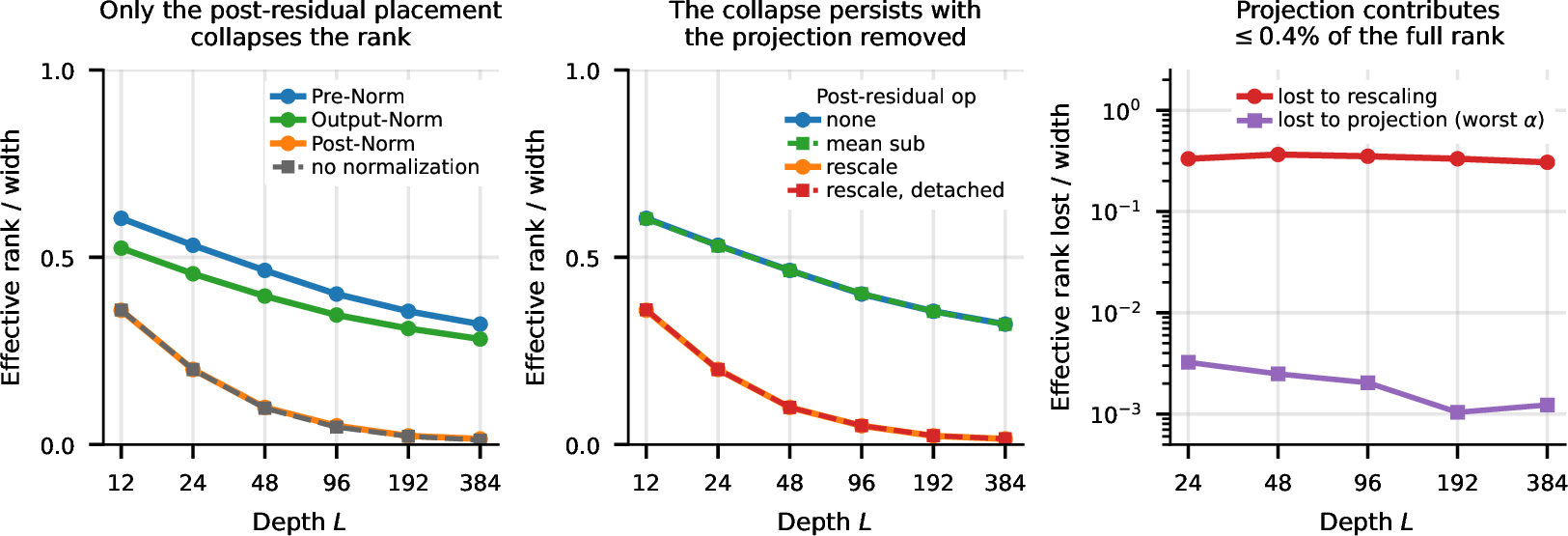
Our experiments present two pieces of evidence that rule out the projection as the cause of the rank collapse. Our first experiment is the placement comparison in Figure 4a: a normalization at the branch input or output keeps a rank floor, while Post-Norm loses rank at the same rate as a network with no normalization at all. A network with no normalization removes no directions, which indicates that the projection is not necessary to induce the collapse. Our second experiment is an ablation that removes the projection from the Jacobian while changing nothing else. The projection term in the RMSNorm Jacobian comes from differentiating through the stream scale. We stop the gradient through that scale to obtain a detached rescaling: the forward pass is unchanged, while the Jacobian becomes a multiple of the identity that removes no direction. This detached rescaling collapses the rank just like ordinary RMSNorm (Figure 4b). When we split the rank that a post-residual RMSNorm removes into a rescaling part and a projection part, the projection accounts for at most \(0.4\%\) of the full rank, across initialization scales (Figure 4c; Appendix 12.2). From this, we conclude that the post-residual normalization does not itself remove rank from the gradient; the placement simply fails to preserve it the way that Pre-Norm does.
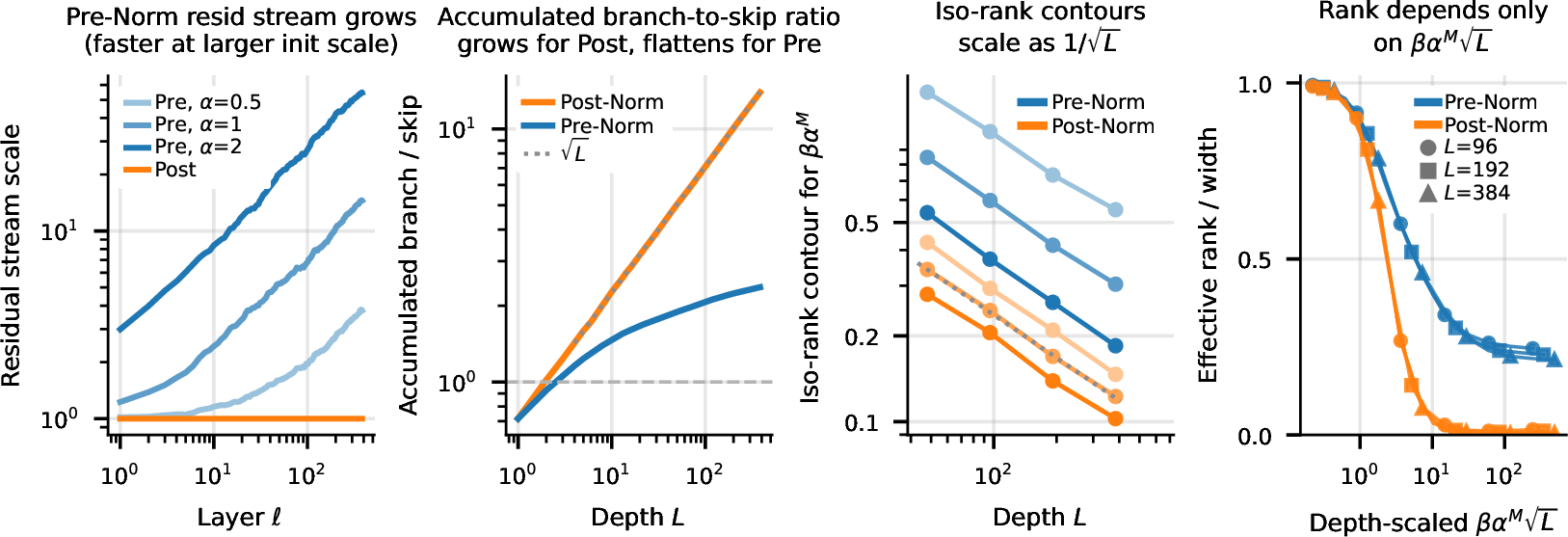
Instead, we show that the normalization placement controls how the branch-to-skip ratio changes across depth, which in turn determines the effective rank. For Pre-Norm and Post-Norm, with the branch scale \(\beta\) and initialization scale \(\alpha\) fixed across layers, the branch-to-skip ratio varies with depth only through the scale of the residual stream. Throughout this section we track its nominal form \(\tilde{r}_\ell \equiv r_\ell / \sqrt{p}\), dropping the constant activation-derivative factor that is shared by every block and both placements (Section 3). In Pre-Norm, the branch acts on a normalized input, so its Jacobian contains the factor \(\sqrt{d}/\|h_\ell\|\) from the normalization (Eq. 8 ), giving \(\tilde{r}_\ell = \beta\alpha^{M}\sqrt{d}/\|h_\ell\|\): the nominal ratio \(\beta\alpha^{M}\) divided by the stream scale \(\mathrm{rms}(h_\ell)\). The Pre-Norm stream grows with depth, since each block adds a branch output of roughly fixed magnitude that is nearly orthogonal to the stream. The scale grows as \(\|h_\ell\| \propto \sqrt{\ell}\) (Figure 5a; Appendix 12.3) and the ratio decays as \(1/\sqrt{\ell}\). In Post-Norm, the rescaling resets the stream to unit scale at every block, and the ratio stays fixed at \(\beta\alpha^{M}\). With no normalization at all, the ratio is also constant, but for a different reason: a degree-one homogeneous branch Jacobian does not depend on the scale of its input, so the growing stream leaves the ratio unchanged.
To see why the branch-to-skip ratio determines the rank, recall from Section 3 that the operations that reduce rank are in the residual branch, and that the skip connection routes the gradient around them. Since the ratio controls how much of the gradient passes through these rank-reducing operations compared to the skip, the rank lost at each layer depends on this ratio. When the ratio decreases with depth, later blocks lose less and less rank, and the rank levels off. When the ratio is constant, every block keeps losing rank, and the rank collapses. This resolves the coincidence in Figure 4a: Post-Norm and no normalization lose rank at the same rate because both hold the branch-to-skip ratio constant across depth.
We now measure how the effective rank depends on the branch-to-skip ratio and the depth together. Recall from Section 3 that networks with the same \(\beta\alpha^{M}\) compute the same function at initialization, and that the effective rank depends on \(\beta\) and \(\alpha\) only through this quantity, for both Pre-Norm and Post-Norm (Figure 2). To measure the depth dependence, we extract iso-rank contours: at each depth \(L\), the value of \(\beta\alpha^{M}\) that holds the effective rank at a fixed level. We find that the effective rank at initialization depends only on the product of the branch-to-skip ratio \(\beta\alpha^{M}\) and a \(\sqrt{L}\) depth factor: for both Pre-Norm and Post-Norm, the iso-rank contours scale as \(1/\sqrt{L}\) (Figure 5c; measured slope \(-0.50\)). Plotted against \(\beta\alpha^{M}\sqrt{L}\), the rank at every depth falls onto one curve for Pre-Norm and another for Post-Norm (Figure 5d): the Post-Norm curve collapses to zero, whereas the Pre-Norm curve approximately plateaus at a moderate level.
We next give a heuristic scaling argument for the \(\sqrt{L}\) depth factor, using the path decomposition in Section 3 (Eq. 5 ). There are \(\binom{L}{k}\) paths of order \(k\), one for each choice of the \(k\) blocks where the path passes through the branch instead of the skip. For Post-Norm, each branch visit contributes a factor of \(\beta\alpha^{M}\) to a path’s norm relative to the skip (we drop the post-residual norm Jacobians, whose projections empirically contribute at most \(0.4\%\) of the full rank). At initialization, the branch Jacobians of different blocks are nearly independent, so the paths of each order add like a random walk, to norm \(\sqrt{\binom{L}{k}}\,(\beta\alpha^{M})^{k} \approx (\beta\alpha^{M}\sqrt{L})^{k}/\sqrt{k!}\). Each additional branch visit multiplies the number of available paths by roughly \(L\), so one factor of \(\sqrt{L}\) comes with each factor of \(\beta\alpha^{M}\). Every order of the expansion then depends on \(\alpha\), \(\beta\), and \(L\) only through \(\beta\alpha^{M}\sqrt{L}\). The effective rank is scale-invariant, so it is a function of this single variable, and the iso-rank contours scale as \(1/\sqrt{L}\).
The order-one paths form the accumulated branch in Figure 5b, where \(L\) randomly oriented terms of magnitude \(\beta\alpha^{M}\) add like a random walk to \(\beta\alpha^{M}\sqrt{L}\) for Post-Norm. For Pre-Norm the growing stream shrinks the per-layer ratios as \(1/\sqrt{\ell}\), and each order of the expansion is again a function of \(\beta\alpha^{M}\sqrt{L}\); the accumulated branch flattens instead of growing (Figure 5b). The rank begins to decrease where the branch orders reach the scale of the skip, around \(\beta\alpha^{M}\sqrt{L} \sim 1\) (the order-one line in Figure 5b). For a more detailed argument, see Appendix 12.3, where we state the assumptions behind each step and validate them empirically, including on GPT-2 Small and Medium both at initialization and after training.
This argument tells us that the rank depends on \(\beta\alpha^{M}\sqrt{L}\), but not how; we measure the shape of each curve empirically (Figure 5d). For Post-Norm, the rank collapses to zero, since the accumulated branch grows as \(\sqrt{L}\) and dominates the skip. For Pre-Norm, the accumulated branch stays comparable to the skip, so the rank plateaus at a moderate level.
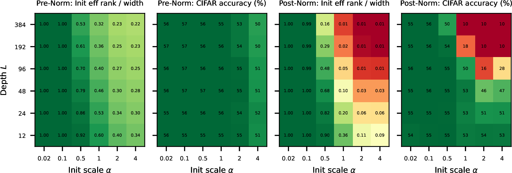
The initialization rank predicts whether these networks train. We train on CIFAR-10 across a grid of initialization scale \(\alpha\) and depth \(L\) for both placements at \(\beta{=}1\), taking the best test accuracy over an Adam learning-rate sweep (Figure 6). We note that CIFAR-10 is an easy task whose accuracy saturates even with a shallow network, so this serves as a coarse test of trainability: it tests whether a configuration trains at all, rather than how it benefits from depth. We see that the networks fail to train in the configurations where the initialization rank collapses: when the rank collapses all the way to 1–2% effective rank over width, the CIFAR accuracy drops toward chance, whereas more moderate rank collapse harms accuracy by several percentage points. Moreover, as depth increases, the learning-rate basin narrows: the maximum stable learning rate decreases with depth as rank collapse begins (Appendix 12.4), whereas the CIFAR accuracy failures occur at larger depths once the rank has fully collapsed. In this sense, the narrowing learning-rate basin acts as an early signal of a trainability problem, before any harm to the final accuracy. We include results for Output-Norm in Appendix 12.5, which are similar to Pre-Norm across the grid.
Our results unify a variety of methods in the normalization placement literature by asking how each changes the branch-to-skip ratio across depth. The Jacobian rank collapse is specific to the post-residual placement. A branch-input or branch-output placement avoids normalizing the residual stream, so the skip remains an identity, the stream grows with depth, and the branch-to-skip ratio decays. Architectures whose per-block normalizations stay off the residual stream [41], [45]–[47] avoid the problem. One line of work aims to revive Post-Norm at depth by up-scaling the skip inside the normalization and/or down-scaling the branch initialization [42], [44]; this shrinks the branch relative to the skip, which in our notation reduces \(\beta\alpha^{M}\) and means a higher initialization rank at every depth (Figure 5d). Additional work reduces how many post-residual normalizations the gradient must pass through [53], [54]. Finally, the \(1/\sqrt{L}\) branch downscaling in Section 3 coincides with our measured iso-rank contours: \(\beta{=}1/\sqrt{L}\) holds \(\beta\alpha^{M}\sqrt{L}\) constant, so it is precisely the scaling at which the initialization rank is depth-invariant, which may be part of why it works well.
This section has shown that the normalization placement and operation determine the Jacobian effective rank at initialization through a single quantity, the branch-to-skip ratio across depth; the projection term in the normalization Jacobian contributes negligible rank loss. The placement determines whether the normalization rescales the residual stream: at the branch input or output, the skip stays an identity, the stream grows, and the ratio decays with depth. Among configurations where a normalization fixes the scale of the branch, the rank collapses only under a post-residual rescaling, the one combination where the branch-to-skip ratio stays constant across depth; every other placement and operation lets the ratio decay, and the rank keeps a floor. Quantitatively, the rank depends on the ratio and the depth only through \(\beta\alpha^{M}\sqrt{L}\), and the initialization rank predicts which configurations train.
Recall from Section 3 that explicitly downscaling the branch with small values of \(\alpha\) or \(\beta\) preserves the rank at a possible cost in composition: short paths through primarily skip connections become dominant, and the network behaves more like an ensemble of shallow subnetworks. Pre-Norm applies this same downscaling implicitly: the stream grows while each branch output keeps a fixed magnitude, so the ratio decays as \(1/\sqrt{\ell}\) and the deep blocks become small perturbations of the identity. Post-Norm instead holds the ratio constant, so its blocks keep transforming the stream and keep losing rank. In Pre-Norm, the rank survives for the same reason the deep layers become ineffective: a near-identity block neither removes directions from the gradient nor adds computation beyond contributing its individual layer to the ensemble. In trained Pre-Norm language models, the deep layers indeed contribute little: they can be pruned individually with minimal performance loss, and their block Jacobians approach the identity [16]. In other words, the decaying branch-to-skip ratio suggests a mechanism for this ineffectiveness, but it also explains the benefit: the rank stays moderate, and the network still trains at depths where Post-Norm fails (Figure 6).


Figure 7: A single uncentered branch matrix grows a mean spike that collapses the forward residual stream rank; a second matrix or a centered activation prevents the collapse. We track the residual stream representation \(Z_\ell\), the matrix whose rows are the representations of \(n\) probe inputs at layer \(\ell\), in a depth-\(L\) network at initialization (Pre-RMSNorm, \(\beta{=}1\), \(d{=}256\), \(L{=}512\), 3 seeds). (a) The mean of \(Z_\ell\) over inputs is the sum \(m_1 + \cdots + m_\ell\) of the per-layer branch means; we plot the alignment \(\cos(m_\ell, m_{\ell+1})\) of consecutive terms. A single uncentered matrix aligns them at the coherence constant \(c_\ell\) (\(1/\pi\) for ReLU, dashed); a second matrix decorrelates them; tanh’s branch means are zero, so there is nothing to align. (b) The norm of that sum grows linearly when the terms align (\(\propto\ell\) guide) and as a random walk when they do not (\(\propto\sqrt{\ell}\)). tanh’s true mean is zero; its curve sits on the gray \(n\)-sample noise floor (Appendix 13). (c) The spectrum of \(Z_L\) at the final layer (top \(16\) of \(d{=}256\) singular values): the top singular value carries the mean, with energy fraction \(1.00\) for M=1 ReLU (a rank-1 spike) and \(0.70\) for M=2 ReLU (a full tail remains); tanh has no spike, and its top direction holds only \(0.08\), barely above the rest of its spectrum. (d) The effective rank of \(Z_\ell\) collapses for M=1 ReLU and stays a finite fraction of the width for M=2 ReLU and tanh..
5 The Two-Matrix Branch and the Coherent Mean Spike↩︎
Transformer feedforward blocks place two weight matrices inside every residual branch. The previous sections might suggest the opposite design: if skip connections restore the rank that branches destroy (Section 3), then perhaps having a skip connection around one matrix per branch would be preferable. In this section, we consider a form of rank collapse in the forward residual stream at initialization that the two-matrix structure prevents. The mean of the residual stream over inputs is a running sum: each layer’s branch adds one term, \(\mu_\ell = m_1 + \cdots + m_\ell\), where \(m_k\) is the mean of layer \(k\)’s branch output. When this sum grows large, it creates a rank-1 mean spike that dominates the spectrum of the representation matrix \(Z_\ell \in \mathbb{R}^{n \times d}\), whose rows are the stream \(h_\ell\) for \(n\) probe inputs, and the representations of all inputs converge to this single direction. When a single uncentered branch keeps these terms aligned across layers, the sum grows linearly with depth, and this spike collapses the rank at moderate depth (Figure 7). We show that two architectural choices prevent this collapse: a second branch matrix decorrelates the terms, or a centered activation avoids the mean spike in the first place. We measure the correlation between the branch means directly and show that it equals the activation moment ratio \(c_\ell = \mathbb{E}[\sigma]^2/\mathbb{E}[\sigma^2]\), and find that a single criterion controls whether an architecture avoids this mean spike collapse: it must remove the aligned component of the branch means.
We first consider the residual stream after a single layer, which [55] show contains a mean spike in the case of an uncentered activation function. At initialization, the branch adds a mean of predictable size to the stream: the weights are isotropic and the Pre-Norm fixes the branch input scale, so each coordinate of the post-activation \(\sigma(Wz)\) has mean \(\mathbb{E}[\sigma]\) and second moment \(\mathbb{E}[\sigma^2]\) over the Gaussian pre-activations. The mean direction therefore carries a fraction \(c_\ell = \mathbb{E}[\sigma]^2/\mathbb{E}[\sigma^2]\) of the post-activation energy, where energy is the squared Frobenius norm. [55] prove that this creates a rank-1 mean spike in the branch-output spectrum for an uncentered activation, whereas a centered activation has zero mean and therefore no spike; \(s_\sigma = 1/c_\ell\) is an upper bound for the stable rank of the branch output, the ratio of total to top-direction energy. Our first contribution in this section is to show the bound is tight at initialization across a set of common pointwise activations: Table 1 lists the constants, and the measured stable rank matches \(s_\sigma\) to within \(6\%\) in every case.
Our main contribution in this section is to show what happens to this mean spike across layers: the spikes of successive layers can align and reinforce one another, or point in unrelated directions and average out. As such, this alignment controls the rate at which the mean spike grows across depth, and therefore the rate of rank collapse: the sum of aligned means grows linearly with \(\ell\), whereas the sum of uncorrelated means is a random walk and grows only as \(\sqrt{\ell}\). Since centered activations avoid this mean spike entirely, we focus on the setting with uncentered activations and consider what happens with one matrix per branch versus two matrices per branch. We find that with one matrix per branch, the correlation between the branch means of any two layers equals the activation moment ratio \(c_\ell\); with two matrices per branch, the second matrix decorrelates the branch means and prevents the rank collapse (Figure 7a; all layer pairs in Figure 14). Across all layer pairs, the measured correlation is \(0.320\) for ReLU (\(1/\pi \approx 0.318\)) and \(0.188\) for GELU (predicted \(c_\ell = 0.187\); Table 1) with one matrix, and zero within noise with two (Appendix 13). To see why a geometric quantity relating two different layers should equal a scalar property of the activation function alone, consider where each layer’s mean comes from: with a single matrix the activation writes directly into the stream, and an uncentered activation has positive mean output in every coordinate, so every layer’s branch mean contains the same component along the all-ones direction, regardless of that layer’s weights. Each mean is this shared component, which carries a \(c_\ell\) fraction of its energy, plus a weight-dependent remainder that is independent across layers; when the means of two layers are correlated, the remainders cancel and only the shared component survives, giving exactly \(c_\ell\). A second matrix removes the shared component: each layer’s \(W_2\) rotates its all-ones part to a different random direction, so the means of different layers share nothing and their correlation is zero. When we measure the mean magnitude across depth, we see the linear mean spike growth for the single-matrix branch (fitted exponent \(0.99\)) and approximately \(\sqrt{\ell}\) growth for the two-matrix branch (fitted exponent \(0.56\)); as expected, the centered activation’s mean is within noise of zero (Figure 7b).
| Activation \(\sigma\) | Centered? | Coherence \(c_\ell=\mathbb{E}[\sigma]^2/\mathbb{E}[\sigma^2]\) | Spike bound \(s_\sigma=1/c_\ell\) | Measured stable rank |
|---|---|---|---|---|
| abs | \(2/\pi \approx 0.637\) | \(\pi/2 \approx 1.57\) | \(1.56\) | |
| ReLU | \(1/\pi \approx 0.318\) | \(\pi \approx 3.14\) | \(3.09\) | |
| GELU | \(0.187\) | \(5.35\) | \(5.16\) | |
| SiLU | \(0.120\) | \(8.33\) | \(7.86\) | |
| tanh | \(0\phantom{.000}\) | \(\infty\phantom{.00}\) | \(50.66\) |
The consequence appears in the spectrum of the representation: by the final layer, the top singular value of the single-matrix branch carries essentially all of the energy (\(1.00\)), whereas the two-matrix branch has a bounded spike (\(0.70\)) and the centered activation has no spike at all (\(0.08\); Figure 7c). What matters for the rank is the energy that remains outside the spike: the two-matrix branch’s remaining \(0.30\) spreads over hundreds of directions, and its effective rank stays near half the width, whereas the single-matrix branch retains essentially nothing and its rank collapses toward zero (Figure 7d). In Appendix 13, we show that this rank collapse is similar across model widths. In Section 3, we show that skip connections preserve the Jacobian rank through their identity terms in the backward pass; the coherent mean spike instead collapses the rank of the forward residual representation, or the skip pathway itself. This is why the feedforward block needs its second matrix: the projection after the activation function decorrelates the means before they are added to the residual stream, preventing this mean spike mechanism for rank collapse.
We note that the backward pass is also a residual stream: the gradient of the loss with respect to each layer’s representation accumulates as \(\delta_{\ell-1} = \delta_\ell + \beta\,J_\ell^\top\delta_\ell\). One might expect a similar spike in the across-input mean of these gradients, but at initialization it does not form: across one matrix, two matrices, and a centered activation, the per-layer contributions are uncorrelated between layers and the gradient stream keeps its rank (Appendix 13). The forward spike comes from the activation’s mean, a fixed direction added at every layer; the backward contribution instead applies the activation’s derivative as a mask and the transposed weights as a rotation, so no shared direction builds up. This decorrelation needs the layers’ weights to be independent, so whether it persists once training couples them is open.
We next consider how normalization layers affect this mean spike, as it would seem that a normalization operation could subtract this mean and prevent the representation collapse. We note, however, that this mean is created by the activation function, so a Pre-Norm operation that centers the branch input does not remove the mean; it would require a normalization operation in the branch after the activation function, before the branch is added to the residual stream. We do find that mean subtraction in the Pre-Norm placement slows the rank collapse, as it breaks a feedback loop in which the stream’s accumulated mean re-enters the branch and reinforces itself. But the collapse still occurs because the activation re-creates the mean at the branch output regardless of its input. A normalization placed after the activation on the branch output can subtract the mean to remove the spike and preserve the rank. It is the mean subtraction in particular that is important here; a rescaling operation like RMSNorm leaves the rank collapse unchanged (Appendix 13). Standard transformer blocks do not need this extra normalization, however, as the second matrix already removes the aligned component of the branch means.
The mean spike could impair training in two ways: through the magnitude it adds to the residual stream, or through the rank it removes from the representation. We train the networks on CIFAR without normalization, and the single-matrix architecture fails to train by about depth 50 whereas the two-matrix architecture fails by about depth 100 (Figure 16). We measure the residual magnitude at initialization and find it grows exponentially with depth, twice as fast for the single-matrix architecture, suggesting its failure at half the depth is due to the faster magnitude growth. Adding Pre-RMSNorm to control the magnitude restores training for both architectures, which reach similar best accuracy over the learning rate sweep (within a point at every depth up to 1000), even though the single-matrix representation has still collapsed to rank around two at initialization. Since CIFAR is a relatively easy task, whether the rank collapse impairs training at larger scale or on harder tasks remains open.
The quantity that determines the representation spectrum at depth is the cross-layer correlation of the branch means. This section showed it equals a scalar property of the activation, \(c_\ell = \mathbb{E}[\sigma]^2/\mathbb{E}[\sigma^2]\). The per-layer stable-rank bound in [55] predicts the conditioning of the gradient, but no per-layer quantity can predict whether the rank survives with depth: a per-layer bound sees the singular values of one layer and not their directions, and the single-matrix and two-matrix branches carry the same per-layer spike and the same per-layer stable rank, diverging only in whether those spikes align across layers. The cross-layer correlation is a single scalar, cheap to measure, and it determines whether the branch means accumulate coherently or average out across depth.
6 Width Expansion and the Full-Rank Branch Threshold↩︎
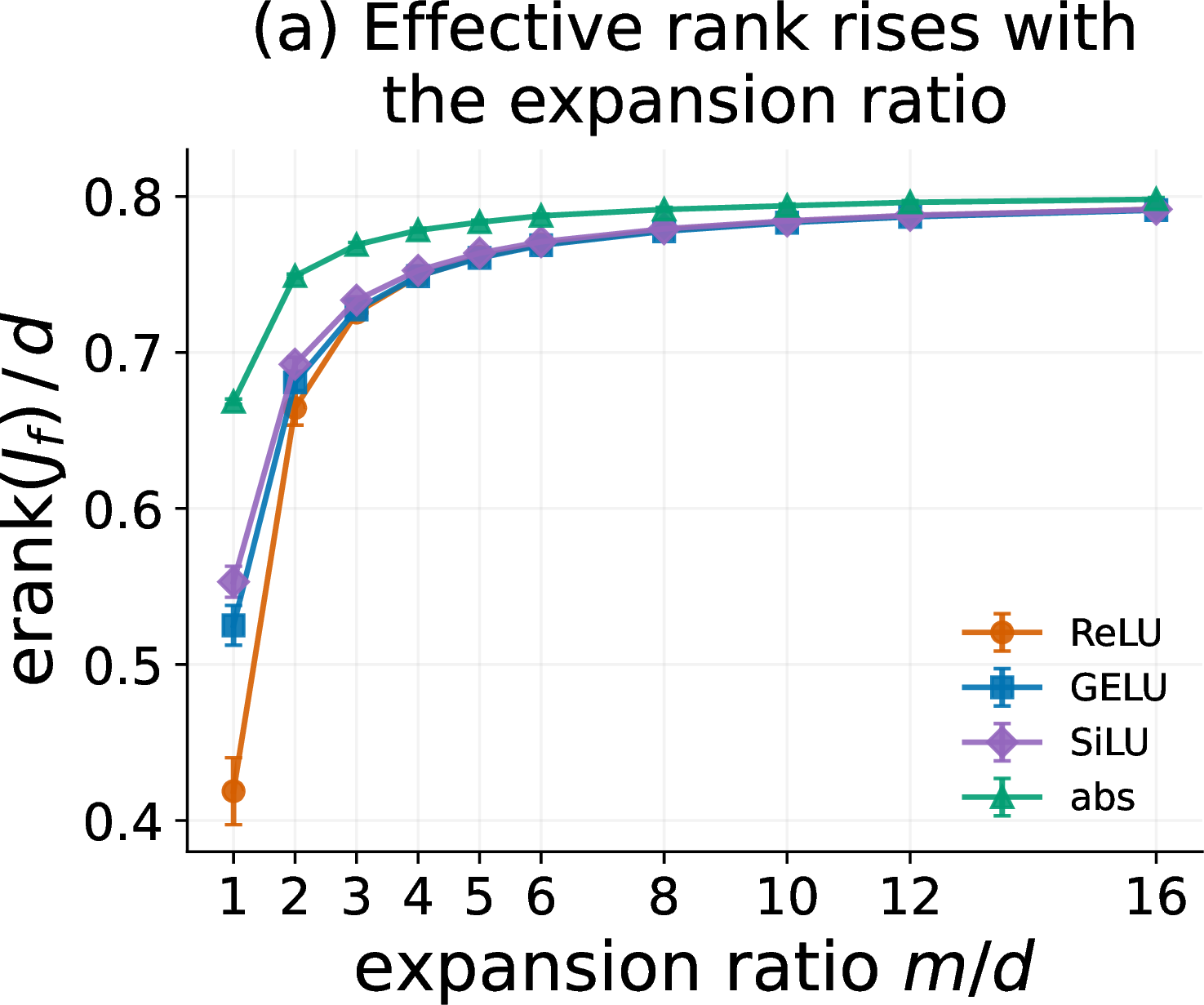
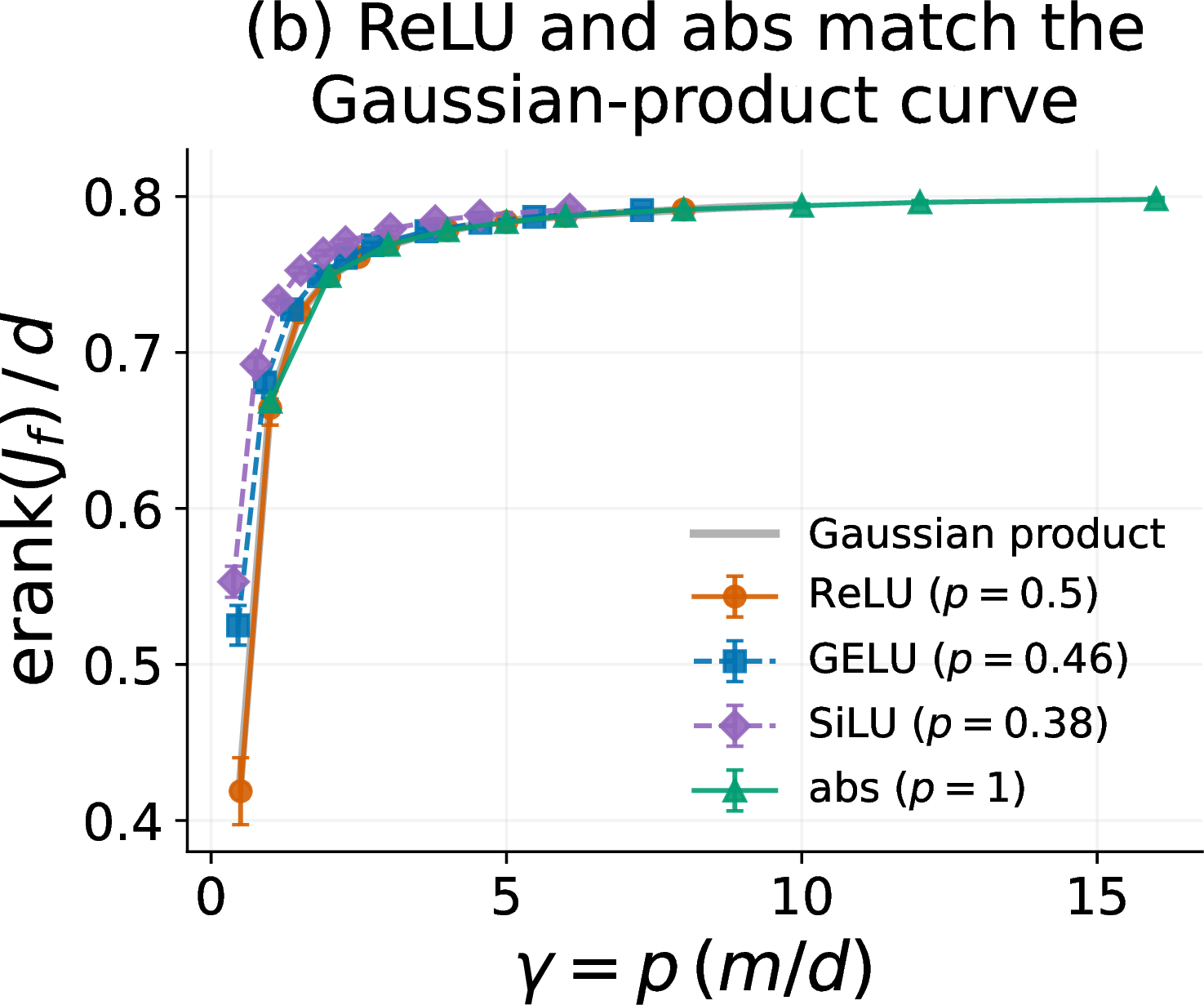
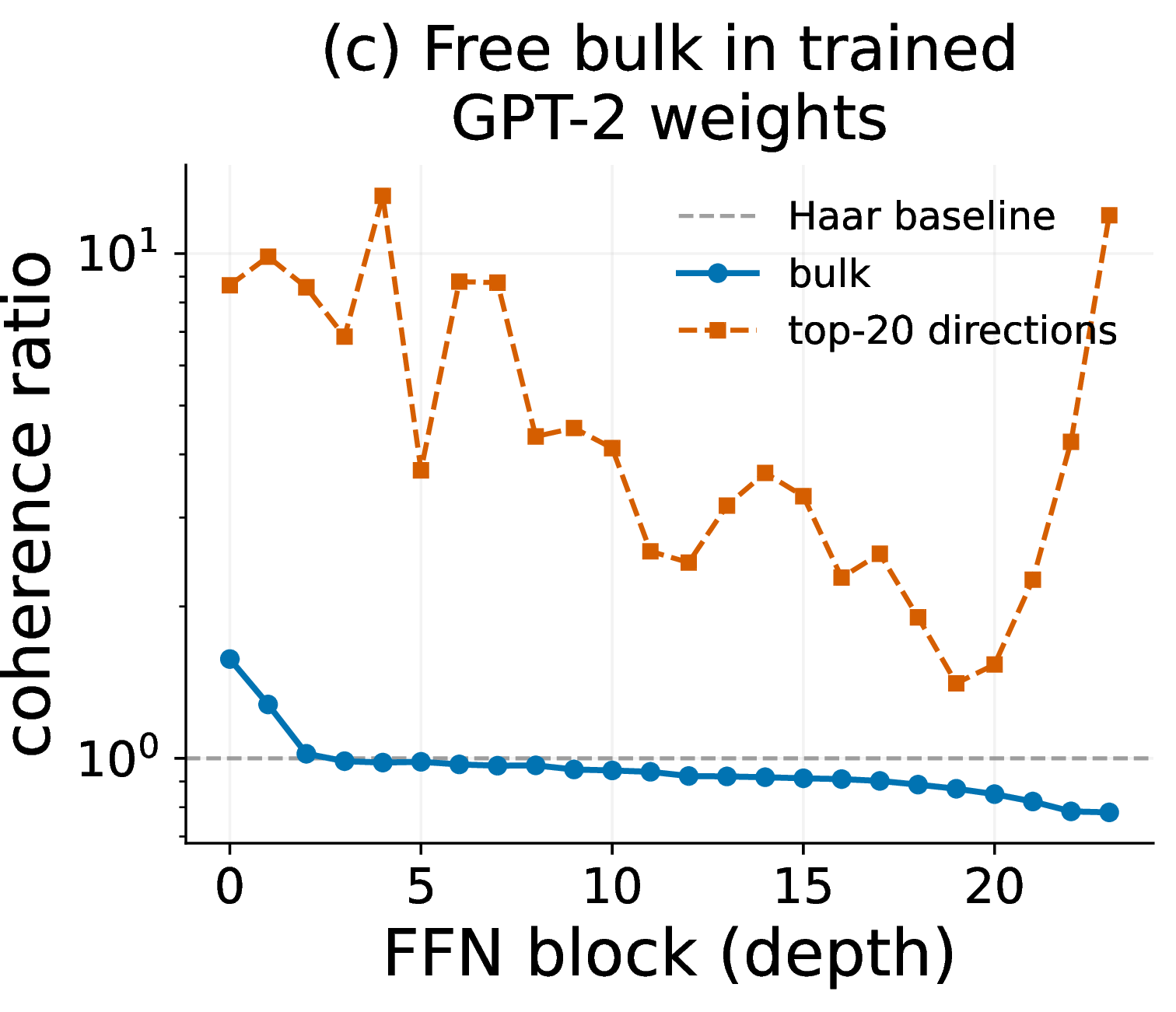
Figure 8: The branch Jacobian’s effective rank increases with the FFN expansion ratio, and a Gaussian-product law predicts it. (a) The normalized effective rank \(\mathrm{erank}(J_f)/d\) increases with the expansion ratio \(m/d\) for ReLU, GELU, SiLU, and abs, fastest for abs (\(p=1\)); GELU and SiLU reach a higher effective rank than ReLU at small expansion ratios despite their smaller \(p\). (b) Plotted against \(\gamma = p\,(m/d)\), ReLU and abs (with \(p\) the survival rate) fall on the effective-rank curve of a product of two Gaussian matrices, while GELU and SiLU (with \(p = \mathbb{E}[\sigma'^2]\)) approach it from above. (c) The prediction assumes \(W_{\mathrm{up}}\) and \(W_{\mathrm{down}}\) are asymptotically free; in pretrained GPT-2 Medium their singular-vector coherence, averaged over all directions, stays close to the Haar baseline of \(1\) across the \(24\) FFN blocks (mean \(0.96\)), so the assumption holds in a trained model. A few extreme directions (the top and bottom \(20\)) are more aligned, but lie outside the bulk that determines the effective rank. \(d = 256\), \(40\) seeds in (a,b); the Gaussian-product curve in (b) uses \(20\) seeds and spans \(\gamma \le 10\)..
![Figure 9: The masked up-projection follows the Marchenko–Pastur law, and its conditioning improves as m/d rises above 1/p. Eigenvalue histogram (filled) of the Gram matrix G = \tfrac{1}{n_{\mathrm{eff}}}(D\,W_{\mathrm{up}})^{\top}(D\,W_{\mathrm{up}}) of the masked up-projection D\,W_{\mathrm{up}} against the Marchenko–Pastur density (line), for ReLU, GELU, and abs (rows) at width expansions m/d \in \{2, 4, 8\} (columns). The mask D = \operatorname{diag}(\sigma'(W_{\mathrm{up}}x)) keeps a fraction p of the m rows, so the survivor count is n_{\mathrm{eff}} = \sum_i \sigma'(z_i)^2 and the aspect ratio is \gamma = n_{\mathrm{eff}}/d. The eigenvalues of G then lie on the support [(1-1/\sqrt\gamma)^2, (1+1/\sqrt\gamma)^2] (dotted edges). At \gamma = 1 (m/d = 1/p, or 2\times for ReLU) the lower edge of the spectrum is zero and D\,W_{\mathrm{up}} is badly conditioned; for \gamma > 1 the spectrum separates from zero. Since W_{\mathrm{down}} is full rank, this submatrix sets \operatorname{rank}J_f. Exact for ReLU and abs (solid), approximate for GELU (dashed). Random Gaussian W_{\mathrm{up}} with unit-variance entries, d = 512, 40 seeds. See Appendix 14 for SiLU.](/article/2607.14018/figures/fig_width_mp_spectrum.png "fig:")
The previous section illustrates why the Transformer feedforward block uses two weight matrices inside every residual branch. In practice, these two matrices have a particular structure: the first matrix expands the width before the activation function is applied, then the second matrix contracts back to the original width. In this section, we ask how this width expansion ratio between the feedforward dimension and model dimension affects the gradient along the residual branch. We write the branch as \(f(x) = W_{\mathrm{down}}\,\sigma(W_{\mathrm{up}} x)\), with up-projection \(W_{\mathrm{up}} \in \mathbb{R}^{m \times d}\) and down-projection \(W_{\mathrm{down}} \in \mathbb{R}^{d \times m}\). We show that the width expansion factor \(m/d\) controls the rank of the branch Jacobian \(J_f\) through the ratio \(\gamma = p(\sigma)\,(m/d)\): the activation mask keeps a fraction \(p(\sigma)\) of the rows in the up-projection matrix, and the surviving submatrix (and hence \(J_f\)) becomes full rank only once \(m/d\) reaches \(1/p(\sigma)\). At this threshold the submatrix is full rank but badly conditioned, as its smallest singular value is near zero (Figure 9). For ReLU, the full-rank threshold is a \(2\times\) expansion, but the \(4\times\) expansion used in practice [1] is much better conditioned.
We can differentiate the branch to write its Jacobian as follows, where \(D\) is a diagonal mask that keeps only the hidden units with nonzero derivative: \[J_f = W_{\mathrm{down}}\, D\, W_{\mathrm{up}}, \qquad D = \operatorname{diag}\!\big(\sigma'(W_{\mathrm{up}} x)\big). \label{eq:jac-factor}\tag{9}\] Let \(p(\sigma)\) denote the expected fraction of the \(m\) rows that survive the mask \(D\); at initialization \(p(\sigma) = \Pr[\sigma'(z)\neq 0]\) for \(z\sim\mathcal{N}(0,1)\), which is one half for ReLU and coincides with the constant \(p = \mathbb{E}[\sigma'(z)^2]\) in Section 3 for masking activations. The Gaussian submatrix formed by the \(pm\) of the \(m\) rows that survive the mask has Gram matrix \(\tfrac{1}{pm}(D\,W_{\mathrm{up}})^{\top}(D\,W_{\mathrm{up}})\), whose eigenvalues follow the Marchenko–Pastur law with aspect ratio \(\gamma = pm/d\), in the proportional limit \(d, m \to \infty\) (Appendix 14). Because \(W_{\mathrm{down}}\) is full-rank and independent of these rows at initialization, it does not reduce the rank of the submatrix, so \(\operatorname{rank}J_f = \operatorname{rank}(D\,W_{\mathrm{up}})\). The \(pm\) surviving rows span the \(d\)-dimensional input space only when \(pm \ge d\), that is \(\gamma \ge 1\). Because the mask fixes the fraction \(p\), widening the branch is the only way to push \(pm\) past \(d\) so that \(D\,W_{\mathrm{up}}\), and therefore \(J_f\), is full rank. The Marchenko–Pastur law gives the spectrum on \([(1-1/\sqrt\gamma)^2, (1+1/\sqrt\gamma)^2]\) (Figure 9), where the lower edge, the smallest eigenvalue, is zero at \(\gamma = 1\) and separates from zero as \(\gamma\) increases. The measured spectra match this prediction exactly for ReLU and abs, and approximately for GELU and SiLU. Setting \(\gamma = 1\) gives the threshold \(m/d = 1/p(\sigma)\), which corresponds to a \(2\times\) width expansion for ReLU. The threshold is correspondingly higher for the smooth activations, about \(2.2\times\) for GELU and \(2.6\times\) for SiLU, with \(p = \mathbb{E}[\sigma'^2]\) as explained below; at \(m/d = 2\) in Figure 9, their spectral lower edge has not separated from zero.
The effective rank of the branch Jacobian increases with the expansion ratio \(m/d\) for all activations (Figure 8a). For activations whose derivative takes only the values \(0\) and \(\pm1\) (ReLU and abs), the masked up-projection \(D\,W_{\mathrm{up}}\) is exactly Gaussian, so \(J_f\) is a product of two Gaussian matrices and we can compute its effective rank as a function of \(\gamma = p\,(m/d)\) (Figure 8b). For these two activations, \(p\) is the survival rate, \(\tfrac12\) and \(1\). For GELU and SiLU, \(\sigma'\) reweights each coordinate instead of masking it, so \(p\) is instead \(\mathbb{E}[\sigma'^2]\), the average squared derivative (\(0.46\) and \(0.38\)); their curves approach the Gaussian-product curve from above (Appendix 14). Because reweighting attenuates directions without removing them, the smooth activations retain more rank than masking at the same \(p\): at small expansion ratios, GELU and SiLU reach a higher effective rank than ReLU despite their smaller \(p\). The Gaussian-product law assumes \(W_{\mathrm{up}}\) and \(W_{\mathrm{down}}\) are free; we measure pretrained GPT-2 and show the bulk singular-vector coherence stays close to the Haar baseline across the 24 FFN blocks (Figure 8c). While the residual skip preserves the rank of the propagated gradient through its identity term, the feedforward width expansion is another architectural factor that controls the rank of the branch Jacobian itself.
7 Related Work↩︎
The literature on dynamical isometry, the condition where every singular value of the input–output Jacobian remains near one so that rank is preserved across depth, shows that narrow conditions on the initializations and activation functions must be satisfied. The Jacobian is a product of weight matrices and activation derivatives, and every factor must be a near-isometry, because the product compounds any spread in the singular values across depth. For the weights, this requires orthogonal initialization, since a matrix with all of its singular values equal to one is orthogonal [19]. For the activations, the derivative must be near-constant in magnitude on the bulk of the preactivation distribution [20], leaving only two categories. Nearly linear activations, with a large linear region around the origin, attain approximate isometry but lack expressivity; absolute-value-like activations achieve perfect isometry but collapse the forward-pass correlations, driving distinct inputs to the same representation [21]. In particular, ReLU has derivative zero on half of its inputs and cannot achieve dynamical isometry. [34] obtain dynamical isometry in residual networks for any activation function by downscaling the branch: this is one end of the tradeoff we study, where a skip-dominated network preserves rank but provides less gradient signal encouraging the layers to compose (Section 3).
Outside these narrow conditions, [18] prove that for layers that are smooth almost everywhere, the rank of the input–output Jacobian can only decrease with depth, and measure this decay in pretrained ResNets, MLP-mixers, and vision transformers. In their exact rank framework, skip connections are a complete fix, because a residual block with a small branch loses no rank at all. The effective rank we track instead degrades continuously through every block, and we quantify how the branch scale, initialization, normalization placement, and width determine how much survives.
Another line of work studies rank collapse along the token dimension, where self-attention drives the representations of all tokens toward a common vector. [25] prove that a network of pure self-attention layers collapses doubly exponentially toward this rank-one state, and that skip connections can counteract the collapse while MLPs only slow it. [17] show that when the token representations collapse at initialization, the gradients of the queries and keys vanish, and they prevent the collapse by scaling the branches by \(1/\sqrt{L}\). [56] attribute the collapse to the spectral gap of the softmax attention matrix, and show that token representations also collapse as the context length grows. Whether the collapse occurs depends on the surrounding components: with LayerNorm the dynamics admit stable equilibria of every rank [57], and with skip connections the outcome is determined by the spectrum of the value and projection weights [58]. Even where skip connections do preserve the token rank, small weights leave the network equivalent to a single attention layer [59]. The same phenomenon appears as over-smoothing in vision transformers and BERT [60], [61]. These results concern the token dimension of attention layers; the rank we study is along the feature dimension, in the gradients and representations of the feedforward blocks. [62] study gradient rank collapse in a third sense, the rank of the weight gradients accumulated over a batch, which is bounded by the narrowest layer width, the batch size, and the linearity of the activation.
Deep residual networks have been shown to behave like ensembles of shallow subnetworks rather than deep networks whose layers compose. [30] decompose the forward pass into \(2^L\) paths that take either the skip connection or the residual branch at each layer, and show that the gradient magnitude is carried mostly by the short paths, while deleting or reordering individual layers barely changes the output of a trained network. [63] use a Taylor series expansion of the forward pass in the residual branch scale, so that a deeper network corresponds to a larger implicit ensemble, and show that controlling the magnitude growth of this expansion by downscaling the branch enables training without normalization. [15] find that the depth scaling exponent of language model loss matches what ensemble averaging would predict, and that the middle layers of trained models make similar, weakly correlated updates. Through a similar path decomposition on the input–output Jacobian, we measure how the gradient magnitude distributes over the path orders, where higher orders pass through more rank-reducing branch operations (Section 3). Ensemble behavior and rank collapse are then the two ends of a single tradeoff, and the branch-to-skip ratio determines where a network falls between them.
The placement of normalization layers has been explored extensively as a design choice: architectures add normalizations at the branch input and output [41], [45], inside the branch [46], [47], on the branch alone [43], varying across depth [48], or in combination [64]. The difficulty of training deep Post-Norm networks has been explained through magnitudes: [65] show that Post-Norm concentrates large gradients near the output at initialization, motivating warmup, and [42] bound the update magnitude to train thousand-layer Post-Norm networks. From the parameterization perspective, [66] tune the depth scaling so that hyperparameters transfer and every layer continues to learn features. Using signal propagation analyses, [67] modify the attention to keep its covariance well-behaved at large depth, [68] train deep transformers without skip connections or normalization, and [69] remove block components without losing training speed. These approaches design for the magnitude and stability of signals and updates; we show that the normalization placement also determines the effective rank, through the branch-to-skip ratio across depth (Section 4). [70] prove that any Pre-Norm network is exactly equivalent to a network with unit-scale stream whose per-layer multipliers preserve the branch-to-skip scale ratio, and use this equivalence to hold activations at unit variance at every depth for low-precision training. We connect the same per-layer ratio, which decays as the Pre-Norm stream grows, to the Jacobian rank.
8 Discussion↩︎
Through the lens of preserving rank across depth, we have seen that the architectural components of the Transformer feedforward block act through two different mechanisms: the first routes much of the gradient around the residual branch through the skip connections, whereas the second increases the rank preserved in the residual branch itself. The two mechanisms act on three distinct rank objects: the first preserves the input–output Jacobian, whereas the second preserves the residual representation and the branch Jacobian.
The first mechanism works around a rank loss that is intrinsic to deep networks: outside the narrow conditions of dynamical isometry [19], [20], every matrix multiplication and activation reduces the rank, and the losses compound with depth. Adding skip connections to MLP layers does not avoid this intrinsic rank loss, since the branch operations remain rank-reducing; instead, the skip connections simply restore the rank periodically by carrying the loss gradient around the branch. Our analysis shows that the more of the gradient that travels through the skip rather than the branch, the more rank survives across depth. A small initialization or small branch scale both reduce the branch-to-skip ratio, routing more of the gradient around the rank-reducing operations.
Normalization layers are usually understood as a way to keep the network magnitudes stable across depth; our analysis shows they also govern rank, by the same routing mechanism as the branch scale. A normalization placed along the residual branch, at the branch input or output, never rescales the residual stream, so the stream grows with depth while each branch adds an increment of fixed scale. The branch then contributes less to the stream in deeper layers, just as a smaller branch scale would, even with residual branch scale \(\beta = 1\). A post-residual rescaling does the opposite, renormalizing the stream at every block and holding its scale fixed, so the branch-to-skip ratio stays constant and the rank collapses with depth. The rank collapse is driven by the branch-to-skip ratio, not the projection terms that appear in the normalization gradient. This perspective on the first mechanism, the routing of the gradient between the branch and the skip, unifies the remedies proposed to prevent rank collapse [17], the conditions under which residual networks achieve dynamical isometry [34], and depth-scaling prescriptions motivated by other goals [32], [33]: each relies on a small branch-to-skip ratio, whether from a small branch scale or a small initialization.
The second mechanism increases the rank the branch itself preserves, through the two-matrix structure of the feedforward block where the first matrix expands the hidden dimension, the activation is applied in the expanded space, and the second matrix contracts back to the original dimension. The two-matrix structure alone, even without the width expansion, prevents the branch means across layers from accumulating coherently: the down-projection matrix decorrelates the branch means, so the mean spike stays bounded and the representation keeps its rank. The width expansion structure plays another important role: intuitively, the up-projection mixes the input directions, so that the elementwise activation that zeros or attenuates some of these mixed directions loses part of many input directions rather than collapsing any single one entirely. This allows the down-projection to recombine, in the original dimension, the directions that survive the activation; the wider the expansion, the higher the branch Jacobian’s effective rank (Section 6).
These two mechanisms illustrate a fundamental tradeoff in architecture design for deep residual networks: even when the residual branch is designed to preserve as much rank as possible when applying matrix multiplications and activation functions, the gradient at each layer flows with some ratio through the rank-reducing operations in the residual branch compared to the rank-preserving identity in the skip connections. If the only objective were to preserve rank in the input–output Jacobian, the trivial solution would be to have all of the gradient flow through the skip connections; however, this makes the network act like an ensemble of layers rather than a deep neural network whose layers learn to compose. This tradeoff reframes the ensemble behavior that prior work observes in deep residual networks [30], [63]: the gradient magnitude concentrates on the short paths through few rank-reducing operations (Section 3), so the same routing that preserves rank is what makes the network behave like an ensemble; under this perspective, the ensemble regime is not simply a pathology but a real alternative to rank collapse. The second mechanism escapes this tradeoff, preserving rank inside the branch rather than routing the gradient around it, but pays for the rank with additional parameters. The feedforward block design then navigates a three-way tradeoff among rank collapse, ensemble-like behavior, and parameter count.
Our perspective on the path decomposition of the input–output Jacobian shows us that the branch-to-skip ratio unifies how the architectural choices, including the initialization scale, residual branch scale, and normalization layers, affect this tradeoff. The choice of the initialization scale and residual branch scale directly control this ratio, but as shown in Section 4, the normalization layers also control the branch-to-skip ratio and therefore indirectly also control this tradeoff. In practice, many frontier models keep the residual branch scale \(\beta = 1\) rather than scaling the branch down (Section 3); this suggests that shifting the gradient too much into the skip connections has empirical disadvantages, perhaps in the network’s ability to compose its layers. [15] find that language model loss improves with depth at the exponent predicted for an ensemble of shallow subnetworks, rather than the faster exponent expected when the layers compose, suggesting that trained language models operate near the ensemble regime. This is consistent with the mechanism in Section 4: even at \(\beta = 1\), Pre-Norm lets the effective branch-to-skip ratio decay with depth, so the deeper layers receive increasingly skip-dominated gradients. On synthetic tasks that require multi-step reasoning, however, deeper transformers outperform shallower but wider models with equal or larger parameter counts [71]. Where a network should sit on this tradeoff is then likely task-dependent: next-token prediction appears well served by the ensemble regime, whereas reasoning requires the layers to compose.
9 Limitations and Future Work↩︎
Our analysis of rank focuses on the feedforward block at initialization, leaving questions about how attention layers and the training process affect the gradient and representation spectra. In principle, mixing across the sequence dimension could offset rank loss by combining representations across positions; in practice, prior work shows that self-attention layers can collapse the token representations toward rank one [25]. Tracking how these spectra evolve during training, and how the optimizer affects them, is a natural extension for future work. We show that the effective rank of the input–output Jacobian predicts CIFAR-10 trainability in Section 4, but as noted there, CIFAR-10 is an easy task that provides only a coarse signal of trainability. A more challenging task, in particular one that requires high-rank representations or sequential composition between layers, could show how the effective rank in the gradient and representation spectra matters in tasks where depth is more genuinely required.
Our derivations explain how each component preserves rank, but leave several specific questions open. For normalization layers, our scaling heuristic argues that \(\beta\alpha^{M}\sqrt{L}\) controls the rank; we measure the shape of the rank curve empirically. For the width expansion, our threshold \(m/d = 1/p\) is exact only for activations whose derivative is \(0\) or \(\pm 1\); our results are approximate for other pointwise activations and we leave gated activations as an open question. Both results could also be applied directly, to predict how deep a normalization placement can scale before its rank collapses and to choose the width-expansion factor that keeps the branch Jacobian full rank for a given activation.
Any neural network architecture that scales depth faces intrinsic rank attenuation for gradients passing through long paths of rank-reducing operations; in deep residual networks, this appears as a tradeoff between rank collapse and ensemble-like behavior. This may induce fundamental limits on the depth-scaling exponents that each architecture family can attain, or possibly universal limits on scaling exponents for neural networks as a whole. At the same time, there may be advantages to mild or moderate amounts of rank loss: limitations on the rank of gradients or representations may provide implicit regularization and improve generalization [72], [73], or act as a useful form of compression [27].
Our path decomposition arguments about gradient signals give some intuition about why skip-dominated gradients may encourage ensemble behavior, but the training dynamics of layer composition are not well-understood. Intuitively, the gradient component through the residual branch tells the feedforward blocks how they should update so that they can cooperatively reduce the loss; in other words, the longer the path, the more the gradient encourages the layers to compose. At the extreme, a network that routes all of its gradient through the skip is a pure ensemble whose layers cannot learn to compose. However, even gradient signal through paths with only several MLP layers may still be sufficient for many layers to gradually learn to compose: if adjacent layers learn to cooperate and progressively pull in their neighbors, deep composition could assemble without gradients ever traversing particularly long paths. Moreover, our path decompositions consider the gradient magnitudes, but gradient signal with small magnitude need not be small in its effect on the function a network learns. Indeed, [74] find that transformers initialized below the typical scale, where the residual branches are weakest, are the ones that converge to compositional rather than memorized solutions, an effect they hypothesize stems from the low-complexity bias of small initializations. Characterizing the relationship between gradient path lengths and how networks actually learn to compose layers is a natural question for future work.
Finally, future work building on our analysis could use spectral properties of the gradient and representation not just to understand how existing architectures work, but to design new architectures and predict how they scale and contend with these fundamental tradeoffs. The tradeoffs we describe likely take different forms in other architecture families, such as recurrent networks and state-space models. Understanding how each component affects these spectra is a step toward combining them into new architectures by design rather than by trial and error.
10 Conclusion↩︎
We have analyzed the modern feedforward block component by component and shown that each one helps preserve the rank of the signals the network propagates across depth: the skip connection routes the gradient around the rank-reducing branch, the placement of normalization sets the branch-to-skip ratio across depth, and with it how much rank survives, the second matrix keeps the representation from collapsing onto a coherent spike, and the width expansion keeps the branch Jacobian full rank. Each of these components was originally motivated by a different purpose — skip connections to prevent vanishing gradients, normalization to control representation magnitudes, the second matrix and width expansion to add capacity — but seen through the lens of rank preservation, they work together to keep the gradient and representation ranks from collapsing with depth. Our analysis is a step toward architecture design that navigates the tradeoff between rank preservation and layer composition as a first principle, and toward understanding fundamental limitations in scaling neural networks.
Acknowledgements↩︎
We thank Leslie Pack Kaelbling for valuable technical discussions. We are grateful to the Google TPU Research Cloud (TRC) program, MIT CSAIL, Phillip Isola, and Kaiming He for providing the compute resources that made this work possible.
11 Skip Connections and the Path Decomposition: Derivations↩︎
This appendix collects the derivations behind Section 3: the path decomposition of the input–output Jacobian (Eq. 5 ), the per-order magnitudes in Figure 3, the recurrence and numerical check behind them, and the argument that the skip must be the identity.
11.1 The path decomposition↩︎
The chain rule turns the residual recurrence \(h_\ell = h_{\ell-1}+\beta f(h_{\ell-1})\) into an ordered product over the \(L\) blocks, \[\frac{\partial h_L}{\partial h_0} = (I+\beta J_L)(I+\beta J_{L-1})\cdots(I+\beta J_1), \qquad J_\ell := \frac{\partial f}{\partial h}\Big|_{h_{\ell-1}}. \label{eq:app-product}\tag{10}\] Each \(J_\ell\) is the branch Jacobian at the forward activation \(h_{\ell-1}\), so the product is evaluated along one forward pass and holds for any differentiable branch.
Distributing the product gives one term per subset \(A\subseteq\{1,\dots,L\}\): each factor contributes either \(I\) or \(\beta J_\ell\), and \(A\) records which blocks contribute the branch. This expands the Jacobian into \(2^L\) paths.
A subset of size \(|A|=k\) carries a factor \(\beta^k\) and a product of \(k\) branch Jacobians. Grouping the \(2^L\) paths by \(k\) defines the order-\(k\) sum \[S_k := \sum_{1 \le \ell_1 < \cdots < \ell_k \le L} J_{\ell_k} \cdots J_{\ell_1}, \qquad \frac{\partial h_L}{\partial h_0} = \sum_{k=0}^{L} \beta^k S_k, \label{eq:app-Sk}\tag{11}\] which is Eq. 5 . The order \(k\) counts the feedforward blocks a path passes through, from \(S_0=I\) (the pure skip) to \(S_L=J_L\cdots J_1\) (every branch). Each \(S_k\) multiplies \(k\) branch Jacobians, so it inherits the rank deficiency of a \(k\)-fold branch composition, weighted by \(\beta^k\).
The order-\(k\) component \(\beta^k S_k\) is the part of the Jacobian built from paths through exactly \(k\) feedforward blocks. We measure its size by the Frobenius norm \(\mu_k := \lVert\beta^k S_k\rVert_F = \sqrt{\sum_i \sigma_i^2}\). The components sum to the Jacobian, \(\sum_k \beta^k S_k = \partial h_L/\partial h_0\), but their norms do not, so each \(\mu_k\) reports one order on its own. Normalizing the \(\mu_k\) to sum to one gives the profile in Figure 3, whose peak (the order of largest magnitude) sits at order three for \(\beta=1\) and at the order-0 skip for \(\beta=1/\sqrt L\) and \(\beta=1/L\).
To efficiently compute the order-\(k\) sum with \(\binom{L}{k}\) terms, we use a dynamic programming algorithm over the blocks. Let \(S_k^{(m)}\) be the sum of order-\(k\) paths through the first \(m\) blocks, so \(S_k = S_k^{(L)}\). An order-\(k\) path through the first \(m\) blocks either takes the skip at block \(m\), leaving an order-\(k\) path through the first \(m-1\) blocks, or takes the branch, extending an order-\((k-1)\) path through the first \(m-1\) blocks by the factor \(J_m\). Block \(m\) has the highest index of the first \(m\) blocks, so the descending-order product puts \(J_m\) on the left: \[S_k^{(m)} = S_k^{(m-1)} + J_m\, S_{k-1}^{(m-1)}, \qquad S_0^{(m)} = I, \quad S_k^{(0)} = 0 \;\;(k \ge 1). \label{eq:app-recurrence}\tag{12}\] Filling the table for \(m=1,\dots,L\) and \(k=0,\dots,L\) computes every \(S_k\) in \(O(L^2)\) matrix multiplications, one per \((m,k)\) cell.
For numerical verification of the recurrence, we draw a random Gaussian input and random weights, compute the Jacobian both by the reconstruction \(\sum_k \beta^k S_k\) and by automatic differentiation of the forward pass, and confirm the two agree to a relative Frobenius error of order \(10^{-15}\). Because the masses \(\mu_k\) span many orders of magnitude, we store each \(S_k\) as a unit-Frobenius matrix and a log-norm scalar and accumulate in log-sum-exp form. Figure 3 reports the \(\mu_k\) and their normalized profile, averaged over 8 seeds, where each seed has its own weight initialization and random Gaussian input; for the initialization-scale panels, the draws are independent at every \((\beta, \alpha)\) grid point.
11.2 Why the skip must be the identity under Pre-Norm↩︎
We reproduce the argument of [29] that the skip connection should be the identity, through the path decomposition above. Consider a residual network where the skip is scaled by a constant \(\lambda\), so that each block is \(h_\ell = \lambda h_{\ell-1} + \beta f(h_{\ell-1})\) and the Jacobian factor becomes \(\lambda I + \beta J_\ell\): \[\frac{\partial h_L}{\partial h_0} = (\lambda I + \beta J_L)(\lambda I + \beta J_{L-1})\cdots(\lambda I + \beta J_1). \label{eq:app-scaled-skip}\tag{13}\] This argument needs the residual stream to pass through each block untouched, which is satisfied by Pre-Norm (but not Post-Norm). Distributing as before, each factor contributes either \(\lambda I\) or \(\beta J_\ell\), so a path of order \(k\) carries \(\lambda^{L-k}\beta^k\), and the order-0 path that stays on the skip at every block is \(\lambda^L I\). This skip path passes through no weights, so its scale \(\lambda^L\) is independent of the network’s weights, at initialization or anywhere in training. The same factor governs both passes: from block \(\ell\), the skip reaches the output through \(L-\ell\) scaled steps, contributing \(\lambda^{L-\ell} h_\ell\) to the forward signal \(h_L\) and \(\lambda^{L-\ell} I\) to the backward Jacobian \(\partial h_L/\partial h_\ell\). Because \(\lambda^{L-\ell}\) is exponential in depth, any \(\lambda \ne 1\) makes the skip path explode (\(\lambda>1\)) or vanish (\(\lambda<1\)), and \(\beta\) cannot correct it because the skip path carries no factor of \(\beta\). Only \(\lambda=1\) holds the skip contribution at \(O(1)\) across depth, which is why the standard residual block fixes the skip to the identity and leaves \(\beta\) as the only free scale.
11.3 Magnitude growth↩︎
Squaring the block \(h_\ell = h_{\ell-1} + \beta f(h_{\ell-1})\) gives the magnitude recurrence \[\lVert h_\ell\rVert^2 = \lVert h_{\ell-1}\rVert^2 + 2\beta\,\langle h_{\ell-1}, f(h_{\ell-1})\rangle + \beta^2\lVert f(h_{\ell-1})\rVert^2. \label{eq:app-magnitude}\tag{14}\] Let \(g_\ell = \lVert f(h_{\ell-1})\rVert / \lVert h_{\ell-1}\rVert\) be the branch gain and \(\rho_\ell = \langle h_{\ell-1}, f(h_{\ell-1})\rangle / (\lVert h_{\ell-1}\rVert\,\lVert f(h_{\ell-1})\rVert)\) the alignment between the branch output and the stream. Then \[\lVert h_\ell\rVert^2 = \lVert h_{\ell-1}\rVert^2\,(1 + 2\beta \rho_\ell g_\ell + \beta^2 g_\ell^2). \label{eq:app-magnitude-factored}\tag{15}\] At initialization the two-matrix branch output is roughly uncorrelated with the stream, so \(\rho_\ell \approx 0\) and the factor is \(1 + \beta^2 g_\ell^2 \ge 1\): the magnitude grows at every block, fastest at \(\beta = 1\) and not at all as \(\beta \to 0\). Whether the growth is additive or multiplicative depends on the gain. Without normalization the branch output scales with its input, \(g_\ell = O(1)\), and the factor compounds to exponential growth in depth. A normalization on the branch input fixes the branch output scale, so \(g_\ell = \lVert f\rVert/\lVert h_{\ell-1}\rVert\) shrinks as the stream grows; the increment \(\beta^2\lVert f\rVert^2\) is then roughly constant and the stream grows additively, \(\lVert h_L\rVert^2 \approx \lVert h_0\rVert^2 + \beta^2\sum_\ell \lVert f\rVert^2 = O(L)\).
11.4 The branch-scale symmetry↩︎
We show that for residual networks with positively homogeneous activations and biasless branches, networks with the same \(\beta\alpha^{M}\) compute the same function at initialization. Write the branch weights as \(W_i = \alpha\bar{W}_i\), for arbitrary matrices \(\bar{W}_i\). Positive homogeneity gives \(\sigma(\alpha z) = \alpha\,\sigma(z)\) for \(\alpha > 0\); applying this identity at each activation, together with the linearity of the matrices, factors the weight scale out of the branch, \[\beta f(x;\, \alpha\bar{W}_1, \ldots, \alpha\bar{W}_M) = \beta\alpha^{M} f(x;\, \bar{W}_1, \ldots, \bar{W}_M). \label{eq:app-symmetry}\tag{16}\] Two configurations of \((\alpha, \beta)\) with the same product \(\beta\alpha^{M}\) therefore compute the same network function, with the same input–output Jacobian and effective rank (Figure 2). In Pre-Norm the normalization acts on the branch input, before the first branch matrix, and in Post-Norm it acts on the stream after the residual addition; in both cases the branch itself is a product of matrices and activations, so the argument applies to either placement.
The equivalence persists throughout training if the optimizer hyperparameters are rescaled accordingly for each matrix. To see why, rescale \(\alpha \gets \lambda\alpha\) and \(\beta \gets \beta/\lambda^{M}\) for some \(\lambda > 0\), which preserves \(\beta\alpha^{M}\). The forward pass is unchanged, but each branch matrix is \(\lambda\) times larger and its gradient is \(\lambda\) times smaller: the gradient with respect to one matrix carries the branch scale \(\beta/\lambda^{M}\) and the other \(M{-}1\) matrices, which contribute \(\lambda^{M-1}\). For the rescaled network to follow the same trajectory, its matrices must remain \(\lambda\) times larger after every update, so the learning rate must be rescaled in accordance with how the gradient changed: \(\eta \gets \lambda^{2}\eta\) for SGD, whose update is proportional to the gradient, and \(\eta \gets \lambda\eta\) for Adam, whose update is invariant to the gradient scale. Similar symmetries were observed for MLP layers in [75], [76] and for the Pre-Norm residual stream in [70]. The rescaling must extend to other optimizer hyperparameters, including \(\epsilon\) in Adam, weight decay, and gradient clipping [76]. This equivalence holds exactly only in infinite precision and infinite dynamic range.
12 Normalization Placement: Additional Results and Derivations↩︎
12.1 Block Jacobians and the normalization projection↩︎
We consider a residual block that may contain a normalization operation in each of three locations [41]: the branch input (\(P\)), the branch output (\(B\)), and the residual stream after the addition (\(R\)). With branch \(f\), the block maps \[h_\ell = R\big(h_{\ell-1} + \beta\,B(f(P(h_{\ell-1})))\big).\] By the chain rule its Jacobian factorizes as \[\frac{\partial h_\ell}{\partial h_{\ell-1}} = J_R\,\big(I + \beta\,J_B J_f J_P\big), \label{eq:block-jac}\tag{17}\] where each \(J\) is the Jacobian of its operation at the relevant point. The placement determines where a normalization Jacobian lands: a branch operation (\(P\) or \(B\)) sits inside the \(\beta\)-scaled branch term, multiplied by the small ratio, whereas the post-residual operation \(R\) multiplies the entire sum, the skip included. This is the structural reason placement matters — only \(R\) applies its Jacobian to the identity path.
12.1.0.1 The RMSNorm Jacobian is a scaled projection.
With its gain at the standard initialization of one, RMSNorm is \(N(x) = \sqrt d\,x/\|x\|\), and \[J_N = \frac{\partial N}{\partial x} = \frac{\sqrt d}{\|x\|}\big(I - \hat{x}\hat{x}^\top\big), \qquad \hat{x} = \frac{x}{\|x\|}. \label{eq:rmsnorm-jac}\tag{18}\] The factor \(\sqrt d/\|x\|\) is the inverse stream scale (the root-mean-square of \(x\) is \(\|x\|/\sqrt d\)); the projection \(I - \hat{x}\hat{x}^\top\) removes the current stream direction \(\hat{x}\).
12.1.0.2 The detached rescaling separates the scale from the projection.
To separate the effect of the projection term from the effect of the scalar rescaling, we define a detached rescaling that divides by the stream scale exactly as RMSNorm does but stops the gradient through that scale: it computes \(x/\operatorname{sg}(\mathrm{rms}(x))\), where \(\operatorname{sg}\) is the stop-gradient. The forward pass is identical to RMSNorm, but the scale is now a constant, so the Jacobian is \[J_{\mathrm{detach}} = \frac{\sqrt d}{\|x\|}\,I, \label{eq:detach-jac}\tag{19}\] the same inverse scale with no projection. It rescales the stream but removes no direction, which is what makes it the control that isolates the rescaling from the projection (Appendix 12.2).
12.1.0.3 The four post-residual operations.
In Table 2 we summarize the four operations we use in the post-residual placement. They let us vary the two factors of a normalization Jacobian independently: the scalar rescaling \(\sqrt d/\|x\|\), which normalizes the stream to unit scale, and the projection \(I - (\cdot)(\cdot)^\top\), which removes a direction. RMSNorm does both; the detached rescaling keeps only the rescaling; mean subtraction keeps only the projection, of a fixed direction and without rescaling; LayerNorm adds mean removal to RMSNorm. Comparing them isolates the contribution of each factor (Appendix 12.2).
| operation | Jacobian | rescales? | removes |
|---|---|---|---|
| RMSNorm | \(\frac{\sqrt d}{\|x\|}\big(I - \hat x\hat x^\top\big)\) | yes | radial \(\hat x\) |
| detached rescale | \(\frac{\sqrt d}{\|x\|}\,I\) | yes | nothing |
| mean subtraction | \(I - \frac1d\mathbf 1\mathbf 1^\top\) | no | fixed \(\mathbf 1\) |
| LayerNorm | \(\frac{\sqrt d}{\|x-\mu\|}\big(I - \hat x_c\hat x_c^\top\big)\big(I - \frac1d\mathbf 1\mathbf 1^\top\big)\) | yes | radial \(+\,\mathbf 1\) |
12.2 The projection is not the primary cause of rank loss↩︎
In Section 4 we observed that the Jacobians of the normalization operations contain projection terms that remove a direction from the gradient: mean subtraction removes the all-ones direction \(\mathbf{1}\), and rescaling removes the current stream direction \(\hat{x} = h/\|h\|\), \[\frac{\partial}{\partial h}\bigl(h - \mu(h)\mathbf{1}\bigr) = I - \tfrac{1}{d}\mathbf{1}\mathbf{1}^{\top}, \qquad \frac{\partial}{\partial h}\,\frac{h}{\mathrm{RMS}(h)} = \frac{\sqrt{d}}{\|h\|}\bigl(I - \hat{x}\hat{x}^{\top}\bigr)\] (Eq. 8 ). Composed over \(L\) layers, these projections could in principle compound into a low-rank Jacobian, which makes the projection terms a natural candidate for explaining the rank collapse [52]. Here we expand on the main-text argument that the projection terms instead have a negligible effect on the rank, and that the branch-to-skip ratio is the primary factor governing the rate of rank loss: we show that the projection is neither necessary nor sufficient for the collapse.
12.2.0.1 The projection is not necessary for rank collapse.
We use the detached rescaling operation to ablate the projection term (Eq. 19 ), which lets us test whether the projection is necessary for the rank collapse to occur. Even with the projection removed, the detached rescaling collapses the rank just like ordinary RMSNorm. Across \(\alpha\in\{0.5,1,2\}\), \(L\in\{48,\dots,384\}\), and \(\beta\in\{1,\,1/\sqrt L\}\), with and without the Pre-RMSNorm, the detached and ordinary ranks differ by at most \(0.4\%\) of the full rank (largest \(0.0039\), at \(\alpha{=}0.5\) and \(\beta{=}1/\sqrt L\), where the rank is near full). Figure 4b overlays the detached and ordinary curves across depth. The projection is therefore not necessary for the collapse.
12.2.0.2 The projection is not sufficient for rank collapse.
Now, to simulate what a projection term without the rescaling would do, we form the product \(\prod_{\ell}(I - x_\ell x_\ell^\top)\) of rank-one projections, where \(x_\ell\) follows an independent random walk on the sphere with step angle \(\epsilon\), so each layer removes a different, uncorrelated direction — the worst case for compounding. The effective rank does not collapse: it stays at \(0.996\) of the width across step sizes \(\epsilon\in[0.01,0.6]\) and depths \(L\in[48,384]\), falling only to \(0.98\) at the largest step and depth (Table 3). Because each removed direction is an independent random vector, it generically does not lie in the range of the accumulated product, so it removes no new dimension and only attenuates the smallest singular values: the product keeps rank \(d-1\) at every depth instead of losing a dimension per layer. Mean subtraction is the opposite extreme, removing the same fixed direction at every layer, which can cost at most one dimension. Direction removal collapses the rank at neither extreme: not when each layer removes an independent direction, and not when every layer removes the same one.
| \(\epsilon\) | \(L{=}48\) | \(L{=}96\) | \(L{=}192\) | \(L{=}384\) |
|---|---|---|---|---|
| \(0.01\) | \(0.996\) | \(0.996\) | \(0.996\) | \(0.996\) |
| \(0.15\) | \(0.996\) | \(0.996\) | \(0.996\) | \(0.996\) |
| \(0.30\) | \(0.996\) | \(0.996\) | \(0.995\) | \(0.995\) |
| \(0.60\) | \(0.994\) | \(0.992\) | \(0.988\) | \(0.980\) |
The collapse is therefore governed by the rescaling, not the projection: keeping the rescaling without the projection still shows rank collapse, whereas applying the projection without the rescaling does not induce the rank collapse.
12.2.0.3 Isolating the post-residual operation.
Figure 4b adds a Pre-RMSNorm to every configuration so that the four post-residual operations are compared on a normalized branch input, varying only the operation. Without a Pre-RMSNorm to control the magnitude, the configurations with no post-residual operation or with mean subtraction have no normalization on the branch at all: their branch-to-skip ratio stays constant, so they collapse at nearly the rate of the rescaling operations and the four become indistinguishable (Figure 10a). To show that this Pre-RMSNorm does not confound our results, Figure 10b shows that with or without it the post-RMSNorm and post-LayerNorm curves coincide.
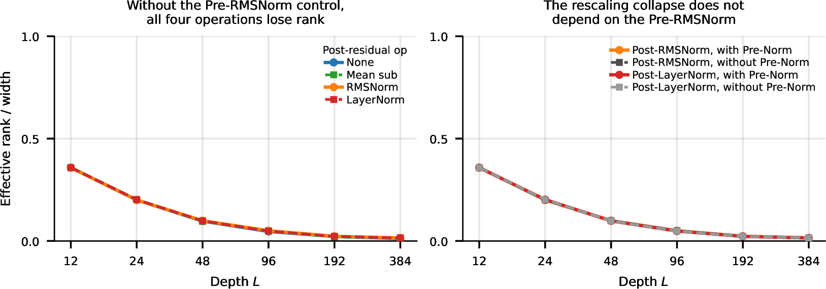
12.3 The depth law: the ratio across depth, contour extraction, and width independence↩︎
12.3.0.1 The branch-to-skip ratio.
The branch-to-skip ratio (Eq. 4 ) is the Frobenius norm of the branch term in the block Jacobian (Eq. 17 ) relative to that of the identity skip. At initialization the branch term \(\beta\,J_B J_f J_P\) collects three factors: the explicit branch scale \(\beta\); a factor \(\alpha^M\) from the \(M\) branch weight matrices, each initialized at scale \(\alpha\), so the branch Jacobian \(J_f\) scales as \(\alpha^M\); and the inverse stream scale \(\sqrt d/\|h_\ell\|\) contributed by the branch normalization (Eq. 18 ), from the branch-input normalization in Pre-Norm or, for a homogeneous branch, equivalently from the branch-output normalization. Their product is \[\tilde{r}_\ell = \frac{\beta\alpha^M\sqrt d}{\|h_\ell\|} = \frac{\beta\alpha^M}{\|h_\ell\|/\sqrt d}, \label{eq:ratio}\tag{20}\] the nominal ratio \(\beta\alpha^M\) divided by the stream scale \(\mathrm{rms}(h_\ell) = \|h_\ell\|/\sqrt d\). As in the main text, we track the nominal form \(\tilde{r}_\ell = r_\ell/\sqrt{p}\), dropping the constant activation-derivative factor \(\sqrt{p}\) (Section 3), which is shared by every block and both placements. The nominal ratio \(\beta\alpha^M\) is \(\tilde{r}_\ell\) at unit stream scale (\(\|h_\ell\| = \sqrt d\)); the per-layer ratio scales inversely with how far the stream has grown. All of the depth dependence enters through \(\|h_\ell\|\): a post-residual rescaling resets it to \(\sqrt d\) at every block, whereas the branch normalizations leave the stream to grow with depth.
12.3.0.2 Residual stream growth.
When the skip connection is an identity (which occurs whenever there is no post-residual normalization), the residual stream is a running sum \(h_\ell = h_{\ell-1} + \beta u_\ell\) of branch outputs \(u_\ell\). The branch input is normalized, so each \(u_\ell\) has roughly fixed magnitude and, at initialization, is nearly orthogonal to the accumulated stream (two generic vectors in \(d\) dimensions have normalized inner product \(O(1/\sqrt d)\)). Expanding, \[\|h_\ell\|^2 = \|h_{\ell-1}\|^2 + 2\beta\langle h_{\ell-1}, u_\ell\rangle + \beta^2\|u_\ell\|^2,\] the cross term vanishes exactly in expectation, since \(W_{\mathrm{down}}\) is zero-mean and independent of the rest of the branch, and the increment \(\beta^2\|u_\ell\|^2\) is constant in expectation. The squared length therefore grows linearly (the magnitude recurrence in Appendix 11): \(\|h_\ell\|^2 = d\,(1+\kappa(\beta\alpha^M)^2\ell)\). The coefficient is \(\kappa = \mathbb{E}[\sigma(z)^2]\), the second moment of the activation values on a unit-variance input, equal to \(\tfrac{1}{2}\) exactly for ReLU. Block \(\ell\)’s branch sees the stream \(h_{\ell-1}\), so the branch-to-skip ratio is \[\tilde{r}_\ell = \frac{\beta\alpha^{M}}{\sqrt{1+\kappa(\beta\alpha^{M})^{2}(\ell-1)}}, \label{eq:ratio-decay}\tag{21}\] which starts near \(\beta\alpha^M\) and decays as \(1/\sqrt\ell\) as the stream grows, whereas a post-residual rescaling resets \(\|h_\ell\| = \sqrt d\) every block and holds the ratio constant at \(\beta\alpha^M\). The measured value, \(\kappa\approx0.51\) for a ReLU branch, matches the derivation: \(\mathrm{rms}(h_\ell)^2-1\) collapses onto a single line in \((\beta\alpha^M)^2\ell\) (Figure 11). \(\kappa\) is a moment of the activation values \(\sigma(z)\), which determine the branch outputs accumulating on the stream. The branch Jacobians are controlled by the derivatives moment \(p = \mathbb{E}[\sigma'(z)^2]\) (Section 3). For ReLU both moments equal \(\tfrac{1}{2}\), by the Gaussian identity \(\mathbb{E}[z^2\mathbf{1}(z>0)] = P(z>0)\). At \(L{=}384\), \(\alpha{=}\beta{=}1\), the stream reaches \(\mathrm{rms}(h_L)\approx 14.5\) for the Pre-Norm input and \(\approx 19.7\) for a unit-increment branch-output normalization, versus \(1.00\) for the post-residual placement.
![Figure 11: At initialization, \mathrm{rms}(h_\ell)^2 grows like 1+\kappa(\beta\alpha^M)^2\ell with \kappa = \mathbb{E}[\sigma^2] = \tfrac{1}{2} for ReLU; the measured \kappa\approx0.51 agrees at every initialization scale. (a) \mathrm{rms}(h_\ell)^2 versus depth for a Pre-Norm two-matrix ReLU branch (both matrices d\times d, d{=}256; \beta{=}1), shown as the measured stream (solid) against the fit (dashed); the stream grows faster at larger \alpha. (b) Plotted against (\beta\alpha^M)^2\ell, \mathrm{rms}(h_\ell)^2-1 collapses onto a single line of slope \kappa\approx0.51 for all \alpha, confirming \|h_\ell\|^2 = d(1+\kappa(\beta\alpha^M)^2\ell).](/article/2607.14018/figures/norm_stream_growth.png "fig:")
12.3.0.3 Networks with post-residual rescaling behave like networks with no normalization.
For a degree-1 positively-homogeneous activation such as ReLU, \(f(ch)=cf(h)\) for \(c>0\), so the branch Jacobian is scale-invariant: \(J_f(ch)=J_f(h)\). This has two consequences. First, a network with no normalization keeps the same stream direction as Post-Norm: by induction, if \(h^{\mathrm{none}}_{\ell-1} = s_{\ell-1}\,\hat{h}^{\mathrm{post}}_{\ell-1}\) for a positive scalar \(s_{\ell-1}\), homogeneity makes the branch outputs match up to \(s_{\ell-1}\), so \(h^{\mathrm{none}}_\ell\) is again a scalar multiple of the Post-Norm sum. The two placements feed their branches the same direction, hence the same \(J_f\). Second, the detached rescaling is the no-norm Jacobian up to a per-layer scalar: its block Jacobian is \(\frac{\sqrt d}{\|\cdot\|}(I + \beta J_f)\) (Eq. 19 ), a scalar times the no-norm block Jacobian \(I + \beta J_f\). The scalars factor out of the product and do not affect the rank, so the detached rescaling and no normalization have identical Jacobian effective rank.
Ordinary Post-Norm adds the projection \(I - \hat{x}\hat{x}^\top\) to each block (Eq. 18 ), the only difference from the detached and no-norm cases. Removing that projection (the detached rescaling, Appendix 12.2) changes the effective rank by at most \(0.4\%\) of the width, so the no-norm, detached, and Post-Norm ranks all coincide to within that margin, and the branch-to-skip ratio is constant \(\beta\alpha^M\) for all three. The degree-1 homogeneity is essential: a degree-2 activation would make \(J_f\) scale as \(\|h\|\), so the no-norm ratio would grow with depth instead of staying constant.
12.3.0.4 The \(\sqrt{L}\) depth factor from path counting.
The path decomposition in Section 3 (Eq. 5 ) writes the input–output Jacobian as a sum over path orders, where the order-\(k\) paths pass through the branch at \(k\) blocks and through the skip everywhere else. For Pre-Norm the decomposition applies directly; for Post-Norm we first drop the post-residual norm Jacobians, whose scalar factors do not change the effective rank and whose projections empirically contribute at most \(0.4\%\) of the width (Appendix 12.2). Relative to the Frobenius norm \(\sqrt{d}\) of the identity skip, a path that visits the branch at blocks \(\ell_1 < \cdots < \ell_k\) has Frobenius norm \(r_{\ell_1}\cdots\, r_{\ell_k}\), the product of the branch-to-skip ratios at the visited blocks, up to an order-one constant per factor that is the same for every \(\alpha\), \(\beta\), and \(L\).
At initialization, the branch Jacobians at different blocks are independent, so distinct paths point in nearly uncorrelated directions and their squared norms add. The order-\(k\) path sum then has relative Frobenius norm \[\Big(\sum_{\ell_1<\cdots<\ell_k} r_{\ell_1}^{2}\cdots\, r_{\ell_k}^{2}\Big)^{1/2} \;\approx\; \frac{\big(\sum_\ell \tilde{r}_\ell^2\big)^{k/2}}{\sqrt{k!}}, \label{eq:orderk-norm}\tag{22}\] where the approximation holds when the individual \(\tilde{r}_\ell^2\) are small. For Post-Norm, \(\tilde{r}_\ell = \beta\alpha^{M}\) at every block, so \(\sum_\ell \tilde{r}_\ell^2 = (\beta\alpha^{M})^2 L\) and the order-\(k\) sum has norm \((\beta\alpha^{M}\sqrt{L})^{k}/\sqrt{k!}\). Each branch visit multiplies a path’s norm by \(\beta\alpha^{M}\) and multiplies the number of available paths by roughly \(L\); a sum of \(N\) randomly oriented terms of equal norm grows as \(\sqrt{N}\) times that norm, so each visit contributes one factor of \(\beta\alpha^{M}\sqrt{L}\). For Pre-Norm, the ratios decay following Eq. 21 , so \[\sum_{\ell=1}^{L} \tilde{r}_\ell^{2} \;\approx\; \int_{0}^{L} \frac{(\beta\alpha^{M})^{2}}{1+\kappa(\beta\alpha^{M})^{2}\ell}\,d\ell \;=\; \frac{1}{\kappa}\,\log\!\big(1+\kappa(\beta\alpha^{M})^{2}L\big), \label{eq:pre-sumr2}\tag{23}\] again a function of \(\beta\alpha^{M}\sqrt{L}\) alone, since \((\beta\alpha^{M})^{2}L = (\beta\alpha^{M}\sqrt{L})^{2}\). In the Frobenius ratio \(r_\ell = \sqrt{p}\,\tilde{r}_\ell\), each order carries an additional factor \((\sqrt{p})^{k}\) and Eq. 23 a prefactor \(p/\kappa\); these shift the collapse onset by the constant \(1/\sqrt{p}\), identically for both placements.
Under three assumptions, which we state below along with measurements that validate them, every order of the expansion depends on \((\alpha,\beta,L)\) only through \(\beta\alpha^{M}\sqrt{L}\); since the effective rank is scale-invariant, it is then a function of this single variable for each placement, and the iso-rank contours scale as \(\beta\alpha^{M} \propto 1/\sqrt{L}\). First, the count \(\binom{L}{k}\approx L^{k}/k!\) requires \(k \ll L\); near the transition at \(\beta\alpha^{M}\sqrt{L} \sim 1\) the contributing orders are small, so this condition is mild. Second, distinct paths are treated as uncorrelated. Each branch Jacobian ends in a zero-mean output matrix, which suppresses correlations between paths, but the activation masks depend on the shared stream, so weak correlations remain; the measured exponents test the net effect, since coherently adding paths would grow the order-\(k\) sum as \((\beta\alpha^{M}L)^{k}/k!\) and give iso-rank contours scaling as \(1/L\), whereas the measured contour slope is \(-0.50\) (Figure 5c) and the order-one sum grows with log–log slope \(0.50\) (Figure 5b), matching the uncorrelated prediction. Third, the Frobenius norms of the path sums do not by themselves determine the rank: we additionally assume that the path sums, normalized by their Frobenius norms, have distributions that do not otherwise depend on \(\alpha\), \(\beta\), or \(L\) (their spectra and their alignments with one another and with the identity). For homogeneous activations like ReLU, \(\alpha\) and \(\beta\) enter each path exactly as the overall factor \((\beta\alpha^{M})^{k}\), so this assumption concerns the depth dependence alone for Post-Norm, and the profile of the decaying ratios for Pre-Norm; the collapse of the measured rank curves onto a single function of \(\beta\alpha^{M}\sqrt{L}\) (Figure 5d) empirically validates that no further dependence on \(\alpha\), \(\beta\), or \(L\) remains. We do not attempt a closed form for the shape of the rank curve: a simple independent-increment model of the spectrum does not match the measurements, with the log-singular-value spread growing faster with depth than the leading order predicts.
12.3.0.5 The assumptions on a real transformer, before and after training.
We test these assumptions on GPT-2 Small and GPT-2 Medium, computing the FFN branch Jacobians analytically along the residual stream of a fixed prompt, both at random initialization and with the pretrained weights (Figure 12). At initialization, every assumption holds exactly: the pairwise cosine similarities between blocks sit at the random-direction baseline of \({\approx}1/d\), and the accumulated branch norm equals the uncorrelated prediction (\(1.00\times\) at \(k{=}L\) for both models). Training induces weak, uniformly positive correlations between blocks (off-diagonal mean \(0.18\) for GPT-2 Small and \(0.15\) for GPT-2 Medium). The accumulated branch reaches \(1.78\times\) and \(2.23\times\) the uncorrelated prediction, against \(3.26\times\) and \(4.59\times\) for fully coherent addition: roughly half of the fully coherent value in both models. The stream growth and the ratio decay persist in direction after training, but the trained stream grows faster, with the growth concentrated in the final blocks. [16] measure the same concentration during pretraining of a 12-layer model, and bound the Pre-LN stream variance between \(\Theta(L)\) and \(\Theta(\exp L)\) under Gaussian independence assumptions; our initialization-versus-trained comparison locates the two ends of this range empirically, with the initialized stream at the linear lower bound, which under their assumptions corresponds to an uncorrelated branch and stream. A faster growing stream suppresses the branch-to-skip ratio further, pushing the deep layers toward the skip-dominated regime rather than toward rank collapse. Two caveats: GPT-2 uses GELU and its stream includes the attention sublayers, so these are measurements of the assumptions rather than of our exact ReLU setting; and the trained per-block profiles vary with the probe token position, whereas the correlation and accumulation measurements do not.
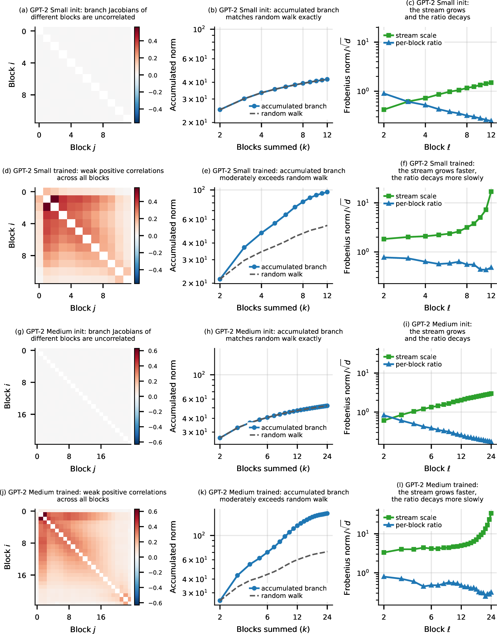
We measure the depth law in Figure 5 as follows. The branch-scale symmetry (Figure 2) lets us vary a single quantity: we fix \(\beta = 1\) and sweep the initialization scale \(\alpha\), so that \(\beta\alpha^M = \alpha^M\). At each depth \(L\) and each rank level \(r^\star\), we extract the iso-rank contour — the value of \(\beta\alpha^M\) at which the effective rank equals \(r^\star\) — by interpolating \(\log\beta\alpha^M\) against the measured rank. Fitting \(\log\beta\alpha^M\) against \(\log L\) then gives the contour’s power-law exponent.
The exponent is close to \(-\tfrac12\) across rank levels and both placements (Table 4), the \(1/\sqrt L\) scaling reported in the main text. The Post-Norm contours are the cleanest, with slopes between \(-0.49\) and \(-0.52\); the Pre-Norm contours are noisier because the rank plateaus near its floor, which flattens the rank–\(\alpha\) curve and makes the crossing harder to locate, but they remain near \(-0.5\).
A wider branch does not change the exponent. Repeating the fit with a \(4\times\) width expansion (a hidden dimension four times the model dimension, both branches having \(M=2\) matrices) leaves the slopes near \(-0.5\) (Table 4, \(4\times\)). The width raises the rank floor at every depth — the per-block conditioning effect in Section 6 — but the depth scaling is unchanged, so the \(\sqrt L\) factor is a property of depth rather than of the per-block branch.
| placement | width | \(r^\star{=}0.4\) | \(r^\star{=}0.5\) | \(r^\star{=}0.6\) |
|---|---|---|---|---|
| Pre-Norm | \(1\times\) | \(-0.46\) | \(-0.50\) | \(-0.52\) |
| Pre-Norm | \(4\times\) | \(-0.57\) | \(-0.47\) | \(-0.48\) |
| Post-Norm | \(1\times\) | \(-0.51\) | \(-0.50\) | \(-0.49\) |
| Post-Norm | \(4\times\) | \(-0.52\) | \(-0.50\) | \(-0.50\) |
12.4 Trainability: the learning-rate basin↩︎
The trainability grid in Figure 6 reports the best CIFAR-10 test accuracy over an Adam learning-rate sweep (\(\eta\) from \(3\times10^{-5}\) to \(10^{-2}\)) at each initialization scale \(\alpha\) and depth \(L\). We also define the maximum stable learning rate as the largest \(\eta\) at which the network still trains, which we take to be a test accuracy of at least \(0.4\) against a chance level of \(0.1\). Table 5 reports the maximum stable learning rate across depth.
Pre-Norm is able to train with all learning rate values in our sweep (up to \(\eta = 10^{-2}\)) at every depth and every \(\alpha\), consistent with its rank floor. The stable learning rate range for Post-Norm instead narrows with depth, and faster at larger \(\alpha\) (Table 5).
The narrowing basin is an early signal of the trainability failure. At \(\alpha = 0.5\) the maximum stable learning rate falls by more than two orders of magnitude across depth (from \(10^{-2}\) to \(3\times10^{-5}\)), yet the best accuracy over the sweep stays at \(0.50\) or above at every depth: the network still trains at a small enough learning rate. At \(\alpha = 1\) the maximum stable learning rate falls thirtyfold by depth 96, and the best accuracy first drops at depth 192 (\(0.18\)), reaching chance at depth 384. The learning-rate basin therefore narrows at a smaller depth than the depth where a loss of accuracy on CIFAR first appears.
| placement | \(\alpha\) | \(L{=}12\) | \(24\) | \(48\) | \(96\) | \(192\) | \(384\) |
|---|---|---|---|---|---|---|---|
| Pre-Norm | all | \(-2\) | \(-2\) | \(-2\) | \(-2\) | \(-2\) | \(-2\) |
| Post-Norm | \(0.5\) | \(-2\) | \(-2\) | \(-2.5\) | \(-3\) | \(-3.5\) | \(-4.5\) |
| Post-Norm | \(1\) | \(-2.5\) | \(-3\) | \(-3.5\) | \(-4\) | — | — |
| Post-Norm | \(2\) | \(-2.5\) | \(-3.5\) | \(-4\) | — | — | — |
| Post-Norm | \(4\) | \(-2\) | \(-3\) | \(-4\) | — | — | — |
12.5 Trainability of Output-Norm↩︎
Figure 4a shows that both branch placements — a normalization at the branch input (Pre-Norm) or the branch output — keep a rank floor, while only the post-residual placement collapses. Output-Norm sits at a marginally lower floor than Pre-Norm, visible in Figure 4a where its curve runs just below Pre-Norm’s: a branch-output normalization fixes every branch increment to unit scale, whereas Pre-Norm’s branch-input normalization feeds the branch a unit input and the ReLU branch contracts it slightly, to a root-mean-square of about \(0.74\). Output-Norm therefore adds a slightly larger increment at each block and runs at a marginally larger branch-to-skip ratio, which lowers its floor. Output-Norm still maintains rank above the threshold where it would harm CIFAR accuracy: across the same grid of initialization scale and depth, its CIFAR-10 accuracy stays near \(55\%\) everywhere, similar to Pre-Norm (Figure 13), unlike Post-Norm, which fails at large \(\alpha\) and depth (Figure 6). A branch-output normalization can still destabilize the residual-stream magnitude at large depth [41], but that is a magnitude effect, separate from the rank-driven failure studied here.
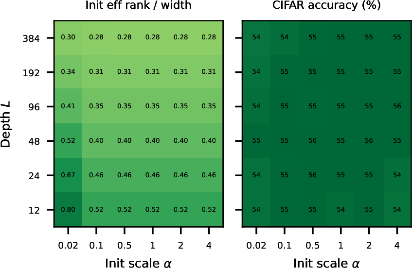
13 Branch Coherence: Derivations and Measurements↩︎
13.0.0.1 The cross-layer correlation equals \(c_\ell\) (spiked regime).
We derive the main-text identity \(\cos(m_\ell, m_{\ell'}) = c_\ell\) for a deep network at initialization, in the regime where the mean spike dominates the residual stream. The branch mean at layer \(\ell\) is \(m_\ell = \mathbb{E}_x[\sigma(W_\ell z)]\), the average of the branch output over inputs, with \(z\) the Pre-Normed branch input and \(W_\ell\) isotropic. Once the spike dominates, the representations of all inputs have collapsed onto its direction, which is the all-ones direction \(\mathbf{1}\): an uncentered activation gives every coordinate of the branch output the same positive mean, so each branch mean carries a \(\mathbf{1}\)-component, and these accumulate until \(\cos(\mu_\ell, \mathbf{1})\to 1\) (verified below). After the Pre-Norm every input then has \(z \approx \mathbf{1}\), independent of \(x\), so the pre-activation of coordinate \(i\) is \[(W_\ell z)_i \;\approx\; (W_\ell \mathbf{1})_i \;=:\; g_i^{(\ell)} .\] The rows of \(W_\ell\) are independent and the Pre-Norm fixes the scale, so the \(g_i^{(\ell)}\) are i.i.d.standard Gaussian and independent across layers. The average over inputs has collapsed — the pre-activation no longer depends on \(x\) – so each branch mean is a deterministic function of that layer’s weights, \(m_\ell[i] \approx \sigma(g_i^{(\ell)})\). The dot product and the norms then concentrate over the \(d\) coordinates, and because \(g^{(\ell)}\) and \(g^{(\ell')}\) are independent for \(\ell\neq\ell'\), \[m_\ell \cdot m_{\ell'} = \sum_i \sigma(g_i^{(\ell)})\,\sigma(g_i^{(\ell')}) \;\to\; d\,\mathbb{E}[\sigma]^2, \qquad \|m_\ell\|^2 = \sum_i \sigma(g_i^{(\ell)})^2 \;\to\; d\,\mathbb{E}[\sigma^2],\] with \(\mathbb{E}[\sigma]\), \(\mathbb{E}[\sigma^2]\) the moments of \(\sigma\) under a standard Gaussian. Hence \[\cos(m_\ell, m_{\ell'}) \;\to\; \frac{\mathbb{E}[\sigma]^2}{\mathbb{E}[\sigma^2]} \;=\; c_\ell .\] The cross term factors into \(\mathbb{E}[\sigma]^2\) because the two layers’ pre-activations are independent: only the part common to every weight draw — the all-ones component, with per-coordinate value \(\mathbb{E}[\sigma]\) — survives the product, and it carries a fraction \(c_\ell\) of the energy \(\mathbb{E}[\sigma^2]\). This is the same \(c_\ell\) that bounds the per-layer stable rank, \(s_\sigma = 1/c_\ell\) (Table 1): the per-layer spike and the cross-layer alignment are one quantity. The collapse \(z \approx \mathbf{1}\) and the concentration of the sums are leading-order statements, exact as the spike grows and \(d \to \infty\).
13.0.0.2 Anchor checks.
The decomposition \(m_\ell = \mathbb{E}[\sigma]\,\mathbf{1} + \varepsilon_\ell\), with \(\varepsilon_\ell\) a zero-mean remainder independent across layers, makes two predictions we confirm at initialization (\(d{=}256\), \(L{=}512\), \(n{=}4096\), 3 seeds). Each branch mean aligns with the all-ones direction at \(\cos(m_\ell, \mathbf{1}) \to \sqrt{c_\ell}\) as depth grows, measured \(0.565\) for ReLU and \(0.433\) for GELU against \(\sqrt{1/\pi} = 0.564\) and \(\sqrt{0.187} = 0.432\); the \(\mathbf{1}\)-component therefore carries a \(\cos^2 = c_\ell\) fraction of the energy. The accumulated mean then aligns fully, \(\cos(\mu_\ell, \mathbf{1})\to 1\), as its \(\mathbf{1}\)-part grows \(\propto\ell\) while the remainder grows only \(\propto\sqrt\ell\). The cross-layer cosine matches \(c_\ell\) directly in Figure 14.
13.0.0.3 No backward analogue.
The forward spike grows because each branch mean contains the weight-independent component \(\mathbb{E}[\sigma]\,\mathbf{1}\), the same direction at every layer. The backward injection has no such component. For a single matrix the branch Jacobian is \(J = \mathrm{diag}(\sigma'(W\hat{z}))\,W\,J_{\mathrm{norm}}\), so the per-layer backward contribution is \[n_\ell = \mathbb{E}_x\!\big[J^\top \delta_\ell\big] = J_{\mathrm{norm}}^\top\, W_\ell^\top\, \mathbb{E}_x\!\big[\sigma'(W_\ell\hat{z})\odot \delta_\ell\big].\] Every term passes through \(W_\ell^\top\), the layer’s own weight matrix, so for two layers \(n_\ell\) and \(n_{\ell'}\) carry \(W_\ell^\top\) and \(W_{\ell'}^\top\) from independent weights: \(\mathbb{E}[n_\ell^\top n_{\ell'}] = 0\) and \(\cos(n_\ell, n_{\ell'}) = O(1/\sqrt d)\to 0\). With no weight-independent shared component, the injections of different layers are mutually random. (Two matrices add a further rotation \(W_2^\top\); a centered activation has no mean to rotate.) The asymmetry is between the mean of \(\sigma\), a fixed direction that is added, and the gain \(\sigma'\), a mask that only scales.
We confirm this at initialization (\(d{=}256\), \(L{=}512\), \(n{=}512\), 3 seeds). We start the backward recursion from two choices of \(\delta_L\), the gradient of the loss with respect to the final representation: a random Gaussian vector per input, in place of any particular loss, and the exact gradient of a softmax cross-entropy loss with a random ten-class head and random labels. In the three branch configurations (one matrix, two matrices, and a centered activation), the cosine similarity \(\cos(n_\ell, n_{\ell'})\) between the backward contributions of two layers averages \(0.00\) over the layer pairs, and its root-mean-square is \(0.063\), which matches the random baseline \(1/\sqrt d = 0.0625\); the forward branch means \(m_\ell\) of the one-matrix ReLU branch align at \(c_\ell = 0.32\). Under the random \(\delta_L\), the \(n \times d\) matrix of gradients \(\delta_\ell\) preserves its rank (\(\mathrm{erank}/d \ge 0.72\), \(\approx 0.9\) for one-matrix ReLU) and grows no mean spike (mean fraction \(\approx 0.002\); the forward mean fraction reaches \(1.0\)). Under the cross-entropy loss, \(\delta_L\) lies in the row space of the ten-class head, so the gradient matrix is effectively rank ten before any layer acts on it. This independence of the per-layer weights is a property of initialization; we do not analyze the trained network.
13.0.0.4 Pairwise alignment across all layer pairs (Figure 14).
The headline result reports the correlation between the branch means of any two layers, while the consecutive-layer panel of Figure 7a shows only neighbors. Figure 14 plots the full matrix \(\cos(m_\ell, m_{\ell'})\), which is flat: for a single uncentered matrix every pair correlates at \(c_\ell\) (off-diagonal mean \(0.320\) for ReLU against \(1/\pi = 0.318\)), and for two matrices or a centered activation every pair sits at zero (off-diagonal mean \(0.002\) and \(-0.000\) respectively). The correlation does not fall off with the layer separation \(|\ell - \ell'|\) because it is carried by one shared direction common to every layer rather than by a chain of layer-to-layer dependences: the all-ones component sits in each branch mean regardless of that layer’s weights, so the alignment is the same at every separation. The main text therefore treats the cross-layer correlation as a single constant \(c_\ell\).

13.0.0.5 Mean-growth exponents and the probe-size control (Figure 7b).
The dashed guides are power laws \(\|\mu_\ell\| \propto \ell^{q}\) anchored at the \(\ell{=}1\) value of each curve, with \(q{=}1\) for the coherent single uncentered branch and \(q{=}\tfrac{1}{2}\) otherwise. A finite probe of \(n\) inputs estimates a zero mean only up to sampling noise: for a zero-mean process the expected measured value is \(\sqrt{\mathbb{E}\|z_\ell\|^2/n}\) (the gray noise floor in the figure), which random-walks across layers at any \(n\) and shrinks only as \(1/\sqrt n\); we therefore vary \(n\) to separate real means from noise. Fitted over \(\ell\in[50,512]\), M=1 ReLU (\(q{=}0.99\), \(\propto\ell\)) and M=2 ReLU (\(q{=}0.56\), \(\propto\sqrt\ell\)) are \(n\)-independent, hence real. SwiGLU likewise has a small but \(n\)-independent mean (\(q{\approx}0.5\)): a gate decorrelates the mean into a random walk rather than removing it. tanh’s apparent \(\sqrt\ell\) instead scales as \(1/\sqrt n\) and vanishes as \(n{\to}\infty\), confirming that a truly centered activation has zero mean; in the figure its curve coincides with the floor. Probe sizes in Figure 7: the mean-magnitude panel uses \(n{=}32768\) so the small real means sit well above the floor; the alignment panel uses \(n{=}4096\); the rank and spectrum panels are \(n\)-independent for \(n{>}d\) and use \(n{=}512\).
13.0.0.6 Width independence (Table 6).
We confirm the collapse is not specific to narrow networks. Table 6 reports the effective rank \(\mathrm{erank}(Z_\ell)/d\) for M=1 ReLU at four widths from \(128\) to \(1024\): the trajectory is nearly width-independent, falling to a few percent of the width by depth \(128\) at every width, and the mean fraction reaches \(1.00\) by the same depth.
| Layer \(\ell\) | |||||
|---|---|---|---|---|---|
| 2-6 Width \(d\) | \(32\) | \(64\) | \(128\) | \(256\) | \(512\) |
| \(128\) | \(0.216\) | \(0.097\) | \(0.044\) | \(0.023\) | \(0.015\) |
| \(256\) | \(0.229\) | \(0.100\) | \(0.040\) | \(0.018\) | \(0.010\) |
| \(512\) | \(0.250\) | \(0.109\) | \(0.040\) | \(0.015\) | \(0.007\) |
| \(1024\) | \(0.296\) | \(0.136\) | \(0.047\) | \(0.015\) | \(0.006\) |
13.0.0.7 Normalization placement (Figure 15).
To understand how normalization placement interacts with this mean spike, we measure the effective rank of the representation under a Pre-Norm and under a branch-output normalization, and find that only a branch-output normalization that subtracts the mean prevents the collapse (Figure 15). In the Pre-Norm placement the rank collapses regardless of the normalizer (panel a): centering the branch input with LayerNorm slows the collapse relative to RMSNorm, because it breaks the feedback loop by which the stream’s accumulated mean re-enters the branch, but the rank still collapses because the activation re-creates the mean at its output. At the branch output, after the activation, the rank is preserved only if the normalization subtracts the mean (panel b): mean subtraction and LayerNorm hold it high, while RMSNorm, which only rescales, collapses identically to no normalization.
Peri-LN [41] proposes a normalization at the branch-output placement in addition to the Pre-Norm. Their experiments use two matrices per branch, so they do not encounter this single-matrix spike.

13.0.0.8 Training scope: the magnitude and rank channels (Figure 16).
We train single-matrix (\(M{=}1\)) and two-matrix (\(M{=}2\)) ReLU networks on CIFAR-10 with Adam for \(5000\) steps (width \(256\), batch \(256\), \(\beta{=}1\)), sweeping the learning rate over six values from \(3{\times}10^{-5}\) to \(10^{-2}\) (the two largest omitted at depths \(500\) and \(1000\), where the optimal rate is smaller) and reporting the best test accuracy over the sweep. The one systematic difference is at the smallest learning rate tested (\(3{\times}10^{-5}\), well below the optimum of \(10^{-3}\)), where the single-matrix architecture trains 4–5 points higher at depths \({\geq}100\); this is consistent with an artifact of the fixed step budget, since the single-matrix network has half as many weight matrices to train at a learning rate this small. The initialization magnitude in panel (b) is the accumulated \(\log_{10}\) of the residual RMS; the per-layer renormalization that keeps it finite at large depth is exact for ReLU, so the two slopes are measured rather than fit.

14 Width Expansion: Full Marchenko–Pastur Derivation↩︎
This appendix derives the results used in Section 6. Sections 14.1–14.3 treat the exact case: we factorize the branch Jacobian, reduce the surviving submatrix to a Marchenko–Pastur ensemble for ReLU and absolute value, and read off the rank threshold \(m/d = 1/p(\sigma)\) and its conditioning. The later subsections cover smooth activations, the freeness assumption and its validation in trained models, the measured spectra of all four activations, the branch Jacobian’s own conditioning, and the Gaussian-product reference curve of Figure 8.
14.1 Jacobian factorization and the survival rate↩︎
The feedforward branch \(f(x) = W_{\mathrm{down}}\,\sigma(W_{\mathrm{up}} x)\), with \(W_{\mathrm{up}} \in \mathbb{R}^{m\times d}\) and \(W_{\mathrm{down}} \in \mathbb{R}^{d\times m}\), has Jacobian \[J_f(x) = W_{\mathrm{down}}\, D(x)\, W_{\mathrm{up}}, \qquad D(x) = \operatorname{diag}\!\big(\sigma'(W_{\mathrm{up}} x)\big). \label{eq:mp-jac}\tag{24}\] The mask \(D(x)\) is diagonal, so it can only lower rank: \(\operatorname{rank}J_f \le \#\{i : \sigma'((W_{\mathrm{up}} x)_i) \neq 0\}\). We call the expected fraction of units with nonzero derivative the survival rate, \(p(\sigma) = \Pr_{z\sim\mathcal{N}(0,1)}[\sigma'(z)\neq 0]\). ReLU has \(\sigma'=\mathbf{1}[z>0]\) and \(p=\tfrac12\); absolute value has \(\sigma'=\mathrm{sign}(z)\) and \(p=1\). At initialization the pre-activations are i.i.d.and mean-zero, so \(D\) keeps \(pm\) rows of \(W_{\mathrm{up}}\) in expectation.
14.2 The surviving submatrix↩︎
For ReLU and absolute value the derivative takes only the values \(0\) and \(\pm1\), so \(D\) either drops a row of \(W_{\mathrm{up}}\) or keeps it at unit magnitude; it never rescales the surviving rows, which is what makes these two activations exact.
For absolute value, \(D = \operatorname{diag}(\mathrm{sign}(W_{\mathrm{up}} x))\) flips the signs of some rows, and the signs cancel in the Gram, \((D\,W_{\mathrm{up}})^{\top}(D\,W_{\mathrm{up}}) = W_{\mathrm{up}}^{\top}W_{\mathrm{up}}\). The surviving submatrix has exactly the spectrum of the full Gaussian \(W_{\mathrm{up}}\), with aspect ratio \(\gamma = m/d\).
For ReLU the surviving rows \(\{w_i : w_i^{\top} x > 0\}\) are Gaussian rows restricted to a half-space. The conditioning gives each a mean \(\sqrt{2/\pi}\,\hat{x}\) along \(\hat{x}=x/\|x\|\) and shrinks its variance there from \(1\) to \(1-\tfrac{2}{\pi}\), while the other \(d-1\) directions stay standard Gaussian. What Marchenko–Pastur needs is only the matrix the Gram converges to, the second moment \(\mathbb{E}[w_i w_i^{\top}\mid w_i^{\top}x>0]\), and there the reduced variance and the squared mean cancel along \(\hat{x}\): \[\mathbb{E}\!\big[w_i w_i^{\top}\mid w_i^{\top}x>0\big] = \underbrace{\big(I - \tfrac{2}{\pi}\hat{x}\hat{x}^{\top}\big)}_{\text{covariance}} + \underbrace{\tfrac{2}{\pi}\hat{x}\hat{x}^{\top}}_{(\text{mean})(\text{mean})^{\top}} = I. \label{eq:mp-second-moment}\tag{25}\] The Gram therefore converges to the identity, and the surviving submatrix is an i.i.d.ensemble with second moment \(I\) and aspect ratio \(\gamma = pm/d = \tfrac12\,(m/d)\).
14.3 Marchenko–Pastur law and the full-rank threshold↩︎
In the proportional limit \(d, pm \to \infty\) with \(\gamma = pm/d\) fixed, the eigenvalues of \(\tfrac{1}{pm}(D\,W_{\mathrm{up}})^{\top}(D\,W_{\mathrm{up}})\) converge to the Marchenko–Pastur law [77] on \([\lambda_-,\lambda_+]\) with \(\lambda_{\pm} = (1 \pm 1/\sqrt{\gamma})^2\). The lower edge \(\lambda_-\) is zero at \(\gamma=1\) and positive for \(\gamma>1\), so the submatrix is full rank if and only if \(\gamma \ge 1\), i.e.\(m/d \ge 1/p(\sigma)\). This threshold \(m/d = 1/p\) equals \(2\) for ReLU and \(1\) for absolute value. At the threshold the submatrix is full rank but its smallest eigenvalue reaches zero, so it is badly conditioned; for \(\gamma>1\) the spectrum separates from zero and the condition number \(\sigma_{\max}/\sigma_{\min} = (1+1/\sqrt\gamma)/(1-1/\sqrt\gamma)\) is finite, falling from \(\infty\) at \(\gamma=1\) to \(5.8\) at \(\gamma=2\) and \(3.0\) at \(\gamma=4\) (the ReLU row of Figure 9, at \(m/d = 2,4,8\)).
The branch Jacobian inherits this rank. Because \(W_{\mathrm{down}}\in\mathbb{R}^{d\times m}\) with \(m \ge d\) is full rank and independent of \(D\,W_{\mathrm{up}}\) at initialization, the column space of \(D\,W_{\mathrm{up}}\) (of dimension \(\operatorname{rank}(D\,W_{\mathrm{up}}) \le d\)) meets the \((m-d)\)-dimensional null space of \(W_{\mathrm{down}}\) only at the origin, so \(\operatorname{rank}J_f = \operatorname{rank}(D\,W_{\mathrm{up}})\). The width threshold for the branch Jacobian is the same as for the surviving submatrix.
14.4 Smooth activations↩︎
For GELU and SiLU the derivative is never exactly zero, so \(D=\operatorname{diag}(\sigma'(W_{\mathrm{up}}x))\) rescales every row rather than dropping any. The Gram becomes \(\tfrac{1}{n_{\mathrm{eff}}}W_{\mathrm{up}}^{\top}\Lambda\,W_{\mathrm{up}}\) with \(\Lambda=\operatorname{diag}(\sigma'(W_{\mathrm{up}}x)^2)\) and \(n_{\mathrm{eff}}=\sum_i\sigma'(z_i)^2\): a Gaussian matrix with a per-row variance profile, not the masked submatrix in Section 14.2.
This \(n_{\mathrm{eff}}\) is the effective number of surviving rows, equal to the count \(pm\) when \(\sigma'^2\in\{0,1\}\). The aspect ratio is then \(\gamma = n_{\mathrm{eff}}/d \to \mathbb{E}[\sigma'^2]\,(m/d)\), so the effective survival rate is the mean squared derivative \(\mathbb{E}[\sigma'^2]\): \(p\) for ReLU and absolute value, \(0.46\) and \(0.38\) for GELU and SiLU.
The spectrum is no longer exactly Marchenko–Pastur: a variance profile deforms the law by the whole distribution of \(\sigma'^2\), not its mean alone [78]. Standard Marchenko–Pastur at \(\gamma=\mathbb{E}[\sigma'^2]\,(m/d)\) matches the scale but not the deformation, a close but inexact fit, and no single scalar survival rate reproduces the spectrum exactly. We use \(\mathbb{E}[\sigma'^2]\), the mean of the weight distribution and the one available in closed form.
14.5 Free-bulk assumption and trained weights↩︎
The effective-rank prediction in Figure 8 composes the spectrum of \(D\,W_{\mathrm{up}}\) with \(W_{\mathrm{down}}\), which requires the two matrices to be asymptotically free: their singular bases in the shared \(m\)-dimensional hidden space should show no systematic alignment. This holds exactly at initialization, where the two are independent Gaussians.
In pretrained GPT-2 Medium we measure the coherence between these bases, normalized so that free bases give \(1\) (Figure 8c). Averaged over all directions it stays close to free across the 24 FFN blocks, with a mean of \(0.96\); the first two blocks are higher (\(1.6\) and \(1.3\)) and the rest fall between \(0.78\) and \(1.02\). The most- and least-aligned twenty directions deviate more (a low-rank trained signal, with coherence near \(5\) at the top and \(3\) at the bottom), but they are a small fraction of the \(1024\) directions and leave the bulk that determines the effective rank approximately free. [79] prove an analogous orthogonalization for BatchNorm; whether it extends to LayerNorm is open, and these measurements are direct evidence that the bulk is close to free in a trained transformer.
14.6 Spectra for all four activations↩︎
Figure 17 overlays the measured Gram eigenvalues on the Marchenko–Pastur density for all four activations at \(m/d\in\{2,4,8\}\). The fit is exact for ReLU and absolute value (solid) and approximate for GELU and SiLU (dashed), as Sections 14.2–14.4 predict. SiLU, deferred from Figure 9, follows the GELU pattern. The smooth-activation deformation in Section 14.4 is visible at small \(m/d\), largest for SiLU at \(m/d = 2\), and shrinks as \(m/d\) grows. At \(m/d = 2\) the smooth activations sit below the full-rank threshold (\(\gamma = p\,(m/d) < 1\)), so the Gram spectrum carries a point mass at zero of weight \({\approx}\,1 - \gamma\), visible as the spike in the first histogram bins, which the continuous Marchenko–Pastur overlay does not include.
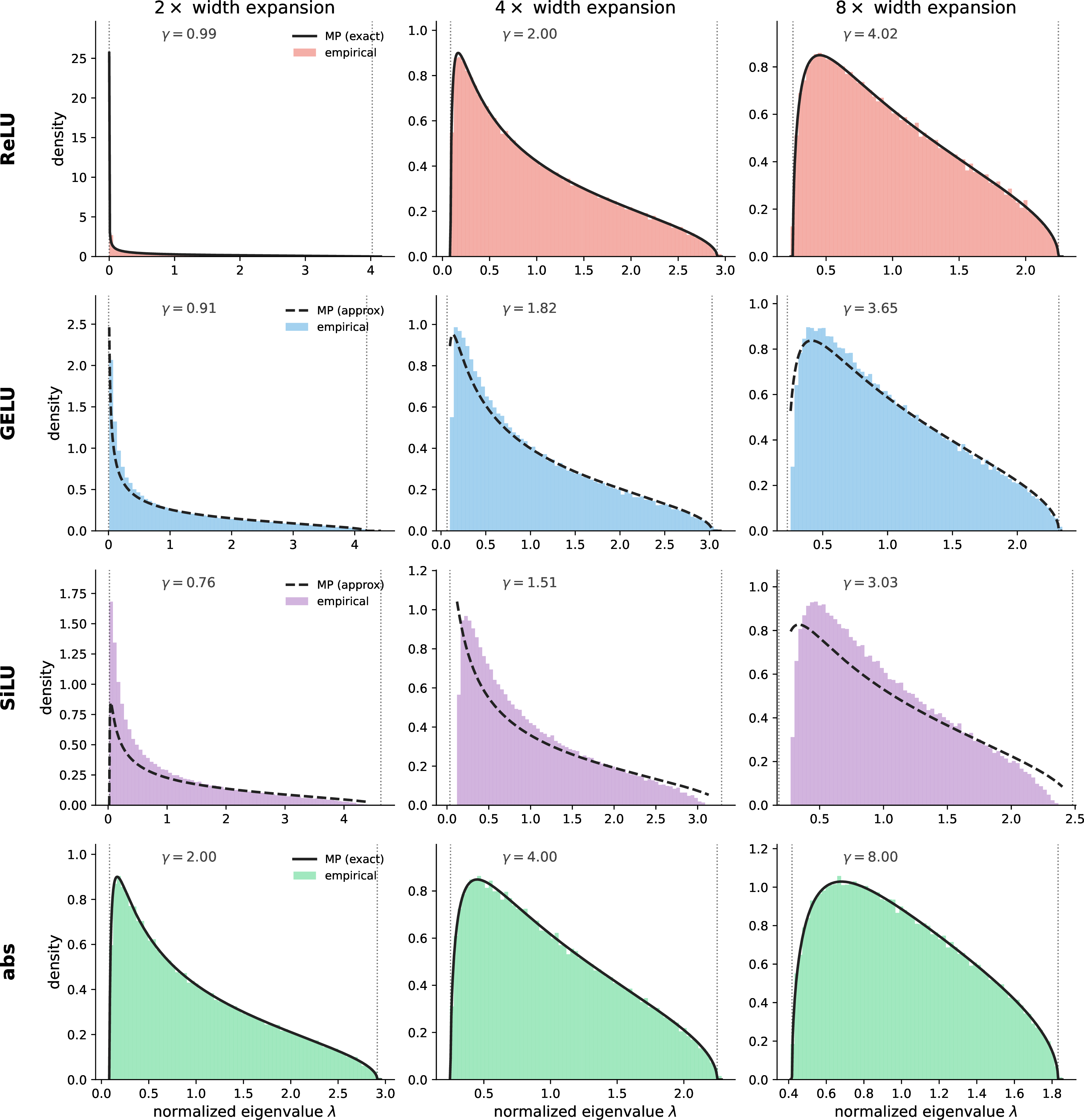
14.7 Conditioning of the branch Jacobian itself↩︎
Above the threshold the submatrix is well-conditioned, but the branch Jacobian \(J_f = W_{\mathrm{down}}(D\,W_{\mathrm{up}})\) is not. Restricted to the \(d\)-dimensional column space of \(D\,W_{\mathrm{up}}\), \(W_{\mathrm{down}}\) acts as a square \(d\times d\) Gaussian, which is poorly conditioned; widening the branch enlarges \(m\) but leaves this \(d\times d\) map unchanged.
The submatrix conditioning improves with width (Figure 9) but the conditioning of the Jacobian \(J_f\) does not: for ReLU at \(d=512\) (weights at the default \(1/\text{fan-in}\) variance), as \(\gamma\) grows from \(2\) to \(16\) the submatrix’s smallest Gram eigenvalue rises from \(0.09\) to \(0.57\), while \(J_f\)’s stays near \(10^{-6}\) even where \(J_f\) is full rank. The effective rank of \(J_f\), however, does improve with width, and the residual skip connection keeps the propagated gradient full rank.
14.8 The Gaussian-product reference curve↩︎
The reference curve in Figure 8b is the effective rank per dimension, \(\mathrm{erank}(J_f)/d\), of a product of two Gaussian matrices (\(W_{\mathrm{up}}\) and \(W_{\mathrm{down}}\) both Gaussian, with no activation) as a function of \(\gamma\). We compute it numerically: at each \(\gamma\) we draw the two factors, form the product, and average \(\mathrm{erank}(J_f)/d\) over seeds (\(d=256\)). The curve rises with \(\gamma\) and reaches \(\approx 0.80\) over the plotted range.
It sits below the surviving submatrix’s effective rank at every \(\gamma\) because the product spreads the spectrum (the same structure behind \(J_f\)’s poor conditioning in Section 14.7), so the branch Jacobian never reaches the effective rank of a single Gaussian matrix, even where it is full rank.