1 Introduction↩︎

1.1 Fixed-rank external fields and covariance Laplacians↩︎

For every positive integer \(r\), write \([r]\mathrel{\vcenter{:}}=\{1,\ldots,r\}\) and let \(\mathbf{1}_r\in\mathbb{R}^r\) denote the all-ones vector. For \(S\subseteq[r]\), write \(\mathbb{I}_S\mathrel{\vcenter{:}}=(\mathbb{I}\{i\in S\})_{i=1}^r\) for its indicator vector, where \(\mathbb{I}\{A\}\) denotes the indicator of a proposition \(A\).

Let \(d\ge2\) be an integer and let \(m\in [d-1]\). Fix \(w=(w_1,\ldots,w_d)\in(0,+\infty)^d\), and let \(\mathsf S\) be an \(m\)-element random subset of \([d]\) distributed according to the rank-\(m\) external-field measure with weights \(w\), i.e., \[\mathbb{P}(\mathsf S=S) = \frac{\prod_{i\in S}w_i}{e_m(w)}, \qquad S\subseteq[d], \quad |S|=m. \label{eq:intro-law}\tag{1}\] Here \[e_m(w) \mathrel{\vcenter{:}}= \sum_{\substack{T\subseteq[d]\\ |T|=m}}\prod_{\ell\in T}w_\ell\] is the \(m\)th elementary symmetric polynomial in \(w_1,\ldots,w_d\). Set \(X\mathrel{\vcenter{:}}=\mathbb{I}_{\mathsf S}\in\{0,1\}^d\). The law 1 is the conditional Bernoulli law, also known as rejective sampling [1]. More explicitly, if \(B_1,\ldots,B_d\) are independent Bernoulli variables with \(\mathbb{P}(B_i=1)=w_i/(1+w_i)\), then \(X\) has the law of \((B_1,\ldots,B_d)^\top\) conditional on \(\sum_iB_i=m\). Equivalently, it is the unique maximum-entropy law among all \(m\)-subset distributions with the same inclusion marginals [2].

Let \[\mu \mathrel{\vcenter{:}}= \mathbb{E}[X], \qquad \Sigma \mathrel{\vcenter{:}}= \operatorname{Cov}(X), \qquad v_i \mathrel{\vcenter{:}}= \Sigma_{ii} = \mu_i(1-\mu_i).\] The fixed-rank identity \(\mathbf{1}_d^\top X=m\) gives \(\Sigma\mathbf{1}_d=0\), so every row of \(\Sigma\) sums to zero. Moreover, Appendix 6 proves that \(\Sigma_{ij}<0\) whenever \(i\ne j\). Define \[c_{ij} \mathrel{\vcenter{:}}= -\Sigma_{ij} > 0 \qquad (i\ne j).\] The zero-row-sum identity gives \[\sum_{j\ne i}c_{ij} = v_i.\] Recall that the weighted Laplacian \(L\) of a graph with edge weights \(c_{ij}\) is defined by \(L_{ij}=-c_{ij}\) for \(i\ne j\) and \(L_{ii}=\sum_{j\ne i}c_{ij}\). Hence \(\Sigma=L\) is the Laplacian of the complete graph with edge weights \(c_{ij}\), and \(v_i\) is the weighted degree of vertex \(i\). Since all edge weights are positive, the graph is connected. Moreover, for every \(x\in\mathbb{R}^d\), \[x^\top\Sigma x = \sum_{i<j}c_{ij}(x_i-x_j)^2.\] We already know that \(\Sigma\mathbf{1}_d=0\). Conversely, if \(x\in\ker\Sigma\), then the displayed sum is zero, so \(x_i=x_j\) along every edge, and connectivity implies that \(x\) is constant. Hence, \(\ker\Sigma=\operatorname{span}\{\mathbf{1}_d\}\).

Let \(\mathbf{e}_1,\ldots,\mathbf{e}_d\) denote the standard basis of \(\mathbb{R}^d\). The Moore-Penrose pseudoinverse \(\Sigma^\dagger\) inverts \(\Sigma\) on \((\ker\Sigma)^\perp\) and vanishes on \(\ker\Sigma\). Equivalently, if \(u\) is an eigenvector of \(\Sigma\) with eigenvalue \(\lambda\ge0\), then \[\Sigma^\dagger u = \begin{cases} \lambda^{-1}u, & \lambda>0,\\ 0, & \lambda=0. \end{cases}\] For \(i\ne j\), the vector \(\mathbf{e}_i-\mathbf{e}_j\) belongs to \(\mathbf{1}_d^\perp\). Since \(\Sigma\) is symmetric and \(\ker\Sigma=\operatorname{span}\{\mathbf{1}_d\}\), we have \(\operatorname{im}\Sigma=\mathbf{1}_d^\perp\). Hence the equation \[\Sigma h = \mathbf{e}_i-\mathbf{e}_j\] has a unique solution \(h\in\mathbf{1}_d^\perp\), namely \(h=\Sigma^\dagger(\mathbf{e}_i-\mathbf{e}_j)\). The standard graph-theoretic quantity effective resistance¹ between \(i\) and \(j\) is defined by \[R_{ij} \mathrel{\vcenter{:}}= (\mathbf{e}_i-\mathbf{e}_j)^\top\Sigma^\dagger(\mathbf{e}_i-\mathbf{e}_j).\] Equivalently, \(R_{ij}=(\mathbf{e}_i-\mathbf{e}_j)^\top h=h_i-h_j\).

Thus the global quantity \(R_{ij}\) is determined by the entire weighted graph. Our main result nevertheless bounds it using only the weighted degrees \(v_i\) and \(v_j\) of the two endpoints.

The statement is uniform in the dimension, the rank, and the external field. Its proof is the main technical contribution of this manuscript.

1.1.0.1 Graph-theoretic interpretation and scope of the bound.

The scale \(1/v_i\) already appears in the simplest graph reductions. If all vertices other than \(i\) are identified, the resulting two-vertex graph has a single edge of total weight \(\sum_{j\ne i}c_{ij}=v_i\). Evaluating the definition of effective resistance on this graph gives \[\left(\sum_{j\ne i}c_{ij}\right)^{-1}=\frac{1}{v_i}.\] For the two-edge path \(i-k-j\) with edge weights \(a\) and \(b\), a direct calculation from the Laplacian gives \[R_{ij} = \frac{1}{a}+\frac{1}{b} = \frac{1}{v_i}+\frac{1}{v_j}.\] Thus, Theorem 1 is a one-sided extension of this exact identity. The resulting upper bound is nevertheless false for general weighted graphs. For example, fix \(d\ge4\), put edge weight \(1\) on the edges of the path \(1-2-\cdots-d\), and put edge weight \(\varepsilon\) on every remaining edge. As \(\varepsilon\downarrow0\), the effective resistance between vertices \(1\) and \(d\) converges to \(d-1\), whereas \[v_1 = v_d = 1+(d-2)\varepsilon, \qquad v_1^{-1}+v_d^{-1} \to 2.\] Therefore, to prove the result we must leverage special characteristics of the fixed-rank covariance Laplacians, and not just the completeness of the given weighted graph. This extra structure appears for example looking at the relative probability of exchanging \(j\) for \(i\), which turns out to be independent of the other selected elements: for every \(T\subseteq[d]\setminus\{i,j\}\) with \(|T|=m-1\), \[\frac{\mathbb{P}(\mathsf S=T\cup\{i\})}{\mathbb{P}(\mathsf S=T\cup\{j\})} = \frac{w_i}{w_j}.\] This identity shows that, after fixing a background set \(T\), the relative likelihood of selecting \(i\) rather than \(j\) is always \(w_i/w_j\). Thus the choice between \(i\) and \(j\) can be analyzed separately from the randomness of the considered background set. For comparison, [3] prove that, for several classes of large random neighborhood graphs, effective resistance is asymptotic to the sum of the inverse endpoint degrees. We remark that their results require specific quantitative connectivity conditions. On the other hand, our Theorem 1 gives instead an exact bound for every dimension, rank, and positive external field. To the best of our knowledge, no previous work gives such a nonasymptotic pairwise effective-resistance bound for rejective sampling.

1.2 A factor-two normalized covariance theorem↩︎

Write \[v = (v_1,\ldots,v_d)^\top, \qquad D = \operatorname{diag}(v_1,\ldots,v_d), \qquad V = \mathbf{1}_d^\top v.\] For symmetric matrices \(A\) and \(B\), write \(A\succeq B\) if \(A-B\) is positive semidefinite. Our Proposition 3 gives the following consequence of Theorem 1.

Anari, Haqi, and Ma conjectured the same normalized spectral statement with lower endpoint \(1\) instead of \(1/2\) [4]. Their first arXiv version stated that stronger assertion as a theorem; the revised version explains that the proposed Hodge-Riemann argument does not establish the normalized eigenvalue bound, and hence they state that correlated-rounding result holds conditionally to the validity of this conjecture [4], [5]. We remark that Corollary 1 is a factor-two relaxation of their Conjecture 3. We remark also that the pairwise resistance bound in Theorem 1 is stronger than this relaxation: it implies the spectral corollary, but the spectral corollary alone would yield only \[R_{ij} \le 2\left(\frac{1}{v_i}+\frac{1}{v_j}\right).\] The sharper resistance bound in Theorem 1 is also the tool used to obtain the static estimate used in the application below.

1.3 Application: correlated sampling on the hypersimplex↩︎

For any two integers \(n\ge1\) and \(k \in \{0, \dots, n \}\), introduce the two pieces of notation \[\Delta^{=}_{n,k} \mathrel{\vcenter{:}}= \left\{x\in[0,1]^n:\sum_{i=1}^n x_i=k\right\} \qquad \text{and} \qquad \Delta^{\le}_{n,k} \mathrel{\vcenter{:}}= \left\{x\in[0,1]^n:\sum_{i=1}^n x_i\le k\right\}.\] The first set is the hypersimplex, and the second is its “at most \(k\)” version. Also write \[\mathcal{S}_{n,k} \mathrel{\vcenter{:}}= \{S\subseteq[n]:|S|=k\}.\] A correlated sampler assigns to each input \(x\in\Delta^{=}_{n,k}\) a random set \(A(x)\in\mathcal{S}_{n,k}\). The sets \(A(x)\) for different inputs are generated using the same random seed, and each coordinate is included with probability given by the corresponding entry of \(x\): \[\mathbb{P}(i\in A(x)) = x_i \qquad \text{for every }x\in\Delta^{=}_{n,k} \text{ and every }i\in[n].\] Its stretch is defined as the smallest constant \(\alpha\) such that \[\mathbb{E}[|A(x)\triangle A(y)|] \le \alpha\|x-y\|_1,\] where \(\triangle\) is the symmetric difference operator, the two outputs \(A(x)\) and \(A(y)\) are generated using the same realization of the sampler’s random seed, and the expectation is taken over this shared randomness. For inputs \(x\in\Delta^{\le}_{n,k}\), the formulation of [6] additionally requires the output cardinality to satisfy \[|A(x)| \in \left\{\left\lfloor\sum_{i=1}^n x_i\right\rfloor,\left\lceil\sum_{i=1}^n x_i\right\rceil\right\}\] for every realization of the common random seed. After an \(O(\log n)\) result of [7], [6] obtained \(O(\log k)\) stretch, independent of the ambient dimension, and asked whether the logarithmic dependence is inherent.

[4] proposed the following canonical scheme. For \(x\in\Delta^{=}_{n,k}\), take the maximum-entropy law \(\mu_x\) on \(k\)-subsets with inclusion marginals \(x\). Draw a uniformly random ordering \((i_1,\ldots,i_n)\) of \([n]\) and, independently, draw mutually independent random variables \(U_1,\ldots,U_n\), each uniformly distributed on \([0,1]\). Process the coordinates in this order. When coordinate \(i_t\) is processed, compute its inclusion probability under \(\mu_x\), conditional on all preceding inclusion and exclusion decisions, and include \(i_t\) if and only if \(U_{i_t}\) does not exceed that probability. The same ordering and the same random variables are reused for every input \(x\). Their analysis provides a constant-stretch guarantee conditional on the validity of two uniform estimates for the covariance Laplacians: a lower bound on the nonzero eigenvalues of the normalized Laplacian and a weighted edge-variation bound for the solutions of the corresponding Laplacian systems with right-hand side \(\mathbf{e}_a-\mathbf{e}_b\). In their work, these estimates were obtained only conditionally to the fact that the normalized covariance conjecture discussed above [4] holds. We do not prove their conjecture. Instead, Corollary 1 establishes the first estimate, while Theorem 1, together with Proposition 4, establishes the second. Therefore, by combining our estimates with their analysis, we obtain a constant-stretch guarantee, without making the assumption of Conjecture 3.

For \(N\ge1\), let \[\Omega_N \mathrel{\vcenter{:}}= \mathfrak S_N\times[0,1]^N,\] where \(\mathfrak S_N\) denotes the set of permutations of \([N]\). We equip \(\Omega_N\) with the product probability measure under which the permutation is uniform on \(\mathfrak S_N\) and the \(N\) coordinates in \([0,1]^N\) are independent and uniformly distributed.

For every \(x\in\Delta^{=}_{n,k}\), we denote by \(\mu_x\) the maximum-entropy law on \(k\)-element subsets with marginals \(x\).

Thus, the constant-versus-\(O(\log k)\) question of [6] has a positive answer.

1.4 Manuscript organization↩︎

The rest of this manuscript is organized as follows. Section 2 first proves Theorem 1. Section 3 then develops two generic consequences of Theorem 1: the half-normalized covariance bound and a weighted edge-variation estimate. Section 4 applies these results to correlated sampling.

2 The proof of our main result↩︎

This section proves Theorem 1 through three main lemmas. First, Lemma 1 controls how the inclusion marginals of an external-field measure vary across three consecutive ranks. Second, Lemma 2 decomposes the inverse effective resistance into an explicit pairwise contribution and a residual regression error. Third, Lemma 3 bounds this regression error by conditioning on two distinct coordinates and applying the adjacent-rank estimate to the remaining coordinates. Finally, we combine these three ingredients to prove Theorem 1.

Fix \(d\ge2\), \(1\le m\le d-1\), and \(w\in(0,+\infty)^d\). Let \(X\) have the law \[\mathbb{P}(X=\mathbb{I}_S)=\frac{\prod_{i\in S}w_i}{e_m(w)}, \qquad |S|=m. \label{eq:fixed-rank-law}\tag{7}\] Write \[\mu = \mathbb{E}[X], \qquad \Sigma = \operatorname{Cov}(X), \qquad v_i = \Sigma_{ii} = \mu_i(1-\mu_i).\] The law has full support, \(\ker\Sigma=\operatorname{span}\{\mathbf{1}_d\}\), and \(\Sigma\) is the Laplacian of a complete positively weighted graph (again, see Appendix 6 for a proof of this fact).

2.1 Adjacent-rank curvature↩︎

Let \(n\ge1\) and let \[z = (z_1,\ldots,z_n)\in(0,+\infty)^n.\] For each \(r\in\{0,\ldots,n\}\), let \(p_r\) be the rank-\(r\) external-field law with weights \(z\). If \(\mathsf S_r\sim p_r\) and \(Y_r=\mathbb{I}_{\mathsf S_r}\), write \[E_r = e_r(z), \qquad \eta_r = \mathbb{E}[Y_r], \qquad \Gamma_r = \operatorname{Cov}(Y_r).\]

2.2 The pair exchange decomposition and the three-slice regression bound↩︎

Assume for now that \(2\le m\le d-2\) and fix \(i\ne j\). For \(u,v\in\{0,1\}\), put \[\pi_{uv} \coloneq \mathbb{P}(X_i=u,X_j=v), \qquad s \coloneq \pi_{10}+\pi_{01},\] and \[\delta \coloneq \pi_{10}-\pi_{01} = \mu_i-\mu_j, \qquad R_{ij} = (\mathbf{e}_i-\mathbf{e}_j)^\top\Sigma^\dagger(\mathbf{e}_i-\mathbf{e}_j),\] and let \(Y=X_{[d]\setminus\{i,j\}}\).

To describe the conditional laws of the background vector \(Y\), we use the notation introduced at the beginning of Subsection 2.1 to the external-field measures on the remaining \(d-2\) coordinates, taking \(n=d-2\) and \(z=w_{[d]\setminus\{i,j\}}\). Conditional on the pair states \(11\), \(10\) or \(01\), and \(00\), the background vector \(Y\) has ranks \(m-2\), \(m-1\), and \(m\), respectively. The states \(10\) and \(01\) induce the same rank-\((m-1)\) law, because their additional weight factors \(w_i\) and \(w_j\) do not depend on the background set. Denote the corresponding means and covariances by \(\eta_{m-2},\eta_{m-1},\eta_m\) and \(\Gamma_{m-2},\Gamma_{m-1},\Gamma_m\). Set \[B \coloneq \pi_{11}\Gamma_{m-2}+s\Gamma_{m-1}+\pi_{00}\Gamma_m, \qquad \kappa \coloneq \eta_{m-2}-2\eta_{m-1}+\eta_m,\] \[\chi \coloneq \kappa^\top B^\dagger\kappa, \qquad \mathcal{D} \coloneq \pi_{11}^{-1}+4s^{-1}+\pi_{00}^{-1}.\]

2.3 The completion of the proof↩︎

3 Implications of the resistance bound↩︎

Let \(C\) be a connected graph Laplacian on \([d]\). Write \[C_{ij} = -c_{ij} \quad (i\ne j), \qquad v_i = C_{ii} = \sum_{j\ne i}c_{ij},\] and put \[v = (v_1,\ldots,v_d)^\top, \qquad D = \operatorname{diag}(v), \qquad V = \mathbf{1}_d^\top v.\] Let \(K=C^\dagger\) and \[R_{ij} = (\mathbf{e}_i-\mathbf{e}_j)^\top K(\mathbf{e}_i-\mathbf{e}_j).\] Throughout this section, assume that the following inequality holds: \[R_{ij} \le \frac{1}{v_i}+\frac{1}{v_j} \qquad \text{for every } 1\le i<j\le d. \label{eq:ER}\tag{12}\]

3.1 Resistance defects and the normalized spectral gap↩︎

Define the resistance defect \[\Delta_{ij} \coloneq \frac{1}{v_i}+\frac{1}{v_j}-R_{ij} \qquad (i\ne j).\]

3.2 Bounds on weighted edge differences↩︎

For any graph Laplacian \(C\), we define the weighted edge-variation seminorm of \(h\in\mathbb{R}^d\) by \[\Phi_C(h) \coloneq \sum_{i<j}c_{ij}|h_i-h_j|.\]

4 Constant-stretch correlated sampling↩︎

In this section, we leverage our results to establish constant-stretch guarantees for the common-seed sampler of [4]. Our main contribution in this part is to make their constant-stretch conclusion unconditional, rather than to prove Conjecture 3: we retain their sampling analysis, but replace the two conjecture-dependent estimates with the bounds proved in this manuscript. More precisely, Proposition 5 makes the dependence of their analysis explicit: a spectral bound with constant \(\rho\) and an edge-variation bound with constant \(\beta\) together imply a stretch bound of \(2\beta/\rho\). The key point is that Propositions 3 and 4 establish these two estimates unconditionally, with \(\rho=1/2\) and \(\beta=4\), respectively. Plugging these values into the Anari-Haqi-Ma analysis gives a constant-stretch guarantee without the need to assume Conjecture 3.

We first define the sampler for inputs \(x\in\Delta^{=}_{n,k}\) satisfying \(0<x_i<1\) for every \(i\in[n]\), i.e., for inputs in the relative interior of the hypersimplex. Appendix 9 defines the sampler on boundary inputs by taking limits of its values at nearby interior points. It then shows that the extended sampler has the same stretch bound and is jointly Borel measurable in the input and the random seed.

4.1 The maximum-entropy sampler↩︎

Recall that \[\mathcal{S}_{n,k} \mathrel{\vcenter{:}}= \{S\subseteq[n]:|S|=k\}.\] For every \(x\in\Delta^{=}_{n,k}\), the entropy-maximization problem over probability laws on \(\mathcal{S}_{n,k}\) with inclusion marginals \(x\) has a unique solution, which we denote by \(\mu_x\).

Suppose that \(0<k<n\) and \(x\in\operatorname{relint}(\Delta^{=}_{n,k})\). For \(\theta\in\mathbb{R}^n\), write \[e^\theta \mathrel{\vcenter{:}}= (e^{\theta_1},\ldots,e^{\theta_n}).\] Define the normalized maximum-entropy parameter by \[\theta(x) \mathrel{\vcenter{:}}= \operatorname*{argmin}_{\theta\in\mathbf{1}_n^\perp}\left\{\log e_k(e^\theta)-x^\top\theta\right\}. \label{eq:maxent-dual-parameter}\tag{14}\] The minimizer in 14 exists and is unique. The corresponding maximum-entropy law is \[\mu_x(S) = \frac{\exp\bigl(\sum_{i\in S}\theta_i(x)\bigr)}{e_k(e^{\theta(x)})}, \qquad S\in\mathcal{S}_{n,k}. \label{eq:external-field-maxent}\tag{15}\] The normalization \(\theta(x)\in\mathbf{1}_n^\perp\) is equivalent to \[\mathbf{1}_n^\top\theta(x) = 0.\]

Define \[\lambda_i(x) \mathrel{\vcenter{:}}= \exp(\theta_i(x)), \qquad i\in[n].\] The first-order optimality condition for 14 states that \[x_i = \frac{\lambda_i(x)e_{k-1}(\lambda_{[n]\setminus\{i\}}(x))}{e_k(\lambda(x))}, \qquad i\in[n]. \label{eq:maxent-marginal-equations}\tag{16}\] Thus 14 , or equivalently 16 together with \(\prod_{i=1}^n\lambda_i(x)=1\), determines the weights used by the sampler.

Under this normalization, \(\theta(x)\) depends smoothly on \(x\). If \(x(t)\) is differentiable with \(x(0)=x\), set \[h \mathrel{\vcenter{:}}= \left.\frac{\mathrm d}{\mathrm dt}\theta(x(t))\right|_{t=0},\] and, further, let \(C_x\) denote the covariance matrix under \(\mu_x\). Since \(x(t) = \mathbb{E}_{\mu_{x(t)}}[X],\) differentiating with respect to \(t\) at \(t=0\) gives the identities \[\dot{x}(0) = C_x\dot{\theta}(0)=C_xh. \label{eq:mean-map-derivative}\tag{17}\] The preceding existence, uniqueness, and smoothness statements are proved in Appendix 8.

We now describe the common-seed sampler of [4]. Fix \(x\in\operatorname{relint}(\Delta^{=}_{n,k})\) and abbreviate \[\lambda_i \mathrel{\vcenter{:}}= \lambda_i(x), \qquad i\in[n].\] The common random seed consists of a uniformly random ordering \((i_1,\ldots,i_n)\) of \([n]\) and independent random variables \(U_1,\ldots,U_n\), each uniformly distributed on \([0,1]\). The same ordering and uniform random variables are reused for every input \(x\).

At each step, the sampler keeps track of three objects: the set \(A\) of coordinates already selected, the set \(R\) of coordinates not yet processed, and the integer \(r\), which indicates how many more coordinates must be selected from \(R\). Conditional on the decisions made so far, the remaining set has the rank-\(r\) external-field law on \(R\) with weights \(\lambda_R\). Consequently, at every nonterminal state \(0<r<|R|\), the conditional inclusion probability of \(i\in R\) is \[p_i(R,r) = \frac{\lambda_i \cdot e_{r-1}(\lambda_{R\setminus\{i\}})}{e_r(\lambda_R)}, \qquad i\in R, \label{eq:conditional-threshold}\tag{18}\] where \(\lambda_R=(\lambda_i)_{i\in R}\).

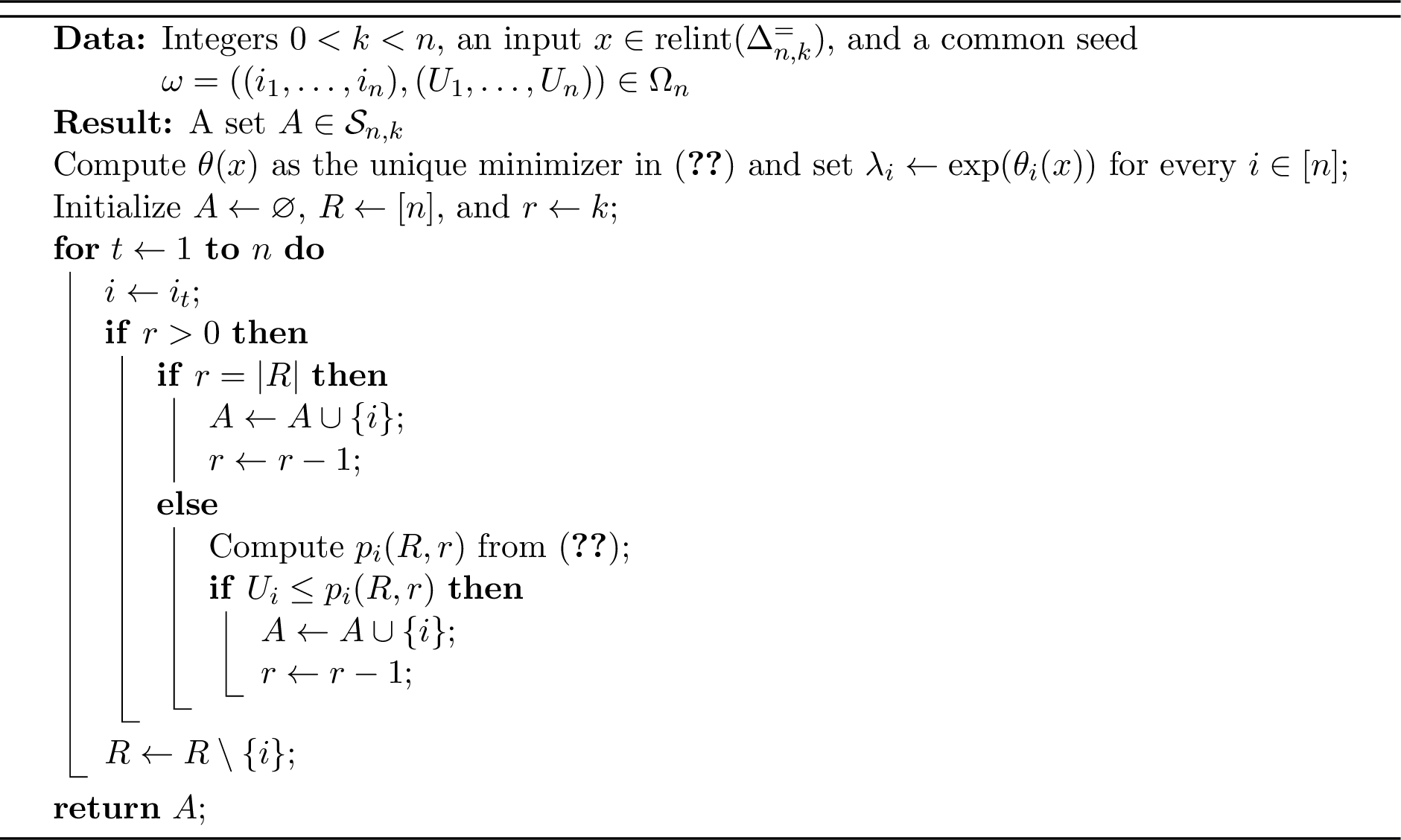
For \(0<k<n\), Algorithm 1 defines the sampler \[A^\circ_{n,k}:\operatorname{relint}(\Delta^{=}_{n,k})\times\Omega_n \to \mathcal{S}_{n,k}.\] By [4], \[A^\circ_{n,k}(x,\cdot)\sim\mu_x\] for every \(x\in\operatorname{relint}(\Delta^{=}_{n,k})\). Quota monotonicity is established in their Lemma 5, while their Lemma 6 shows that, after the first opposite decision, the two fixed-field continuations differ in exactly two final coordinates.

Algorithm 1 does not directly apply to boundary inputs, because the finite parameter \(\theta(x)\) in 14 need not exist there. To extend the sampler, let \[u = \frac{k}{n}\mathbf{1}_n, \qquad x^\varepsilon = (1-\varepsilon)x+\varepsilon u.\] For every \(x\in\Delta^{=}_{n,k}\), \[\mu_{x^\varepsilon} \to \mu_x \quad \text{in total variation as }\varepsilon\downarrow0. \label{eq:radial-law-continuity}\tag{19}\] This continuity statement is proved in Appendix 8.

The sampler \(A_{n,k}\) in Corollary 2 is the boundary completion of \(A^\circ_{n,k}\) constructed in Appendix 9. Specifically, for \(q\ge1\), the appendix defines \[x^{(q)} = (1-2^{-q})x+2^{-q}u, \qquad A_q(x,\omega) = A^\circ_{n,k}(x^{(q)},\omega).\] For every fixed \(x\), the sequence \((A_q(x,\omega))_{q\ge1}\) is eventually constant almost surely. The completed sampler is defined to be its eventual value whenever that value exists and a fixed default \(k\)-element set otherwise. It follows from the proof in Appendix 9 that the map \(A_{n,k}\) so defined is jointly Borel measurable, exactly samples from \(\mu_x\), and preserves the stretch bound.

4.2 From covariance estimates to a stretch bound↩︎

For each nonterminal conditional law of the sampler, let \(q\) be the number of remaining coordinates. After relabeling these coordinates by \([q]\), let \(C\in\mathbb{R}^{q\times q}\) denote its covariance matrix, and put \[D \mathrel{\vcenter{:}}= \operatorname{diag}(C_{11},\ldots,C_{qq}).\] For every \(h\in\mathbb{R}^q\), define \[\Phi_C(h) \mathrel{\vcenter{:}}= \sum_{1\le i<j\le q}(-C_{ij})|h_i-h_j|.\] Now fix an interior input \(x\), set \(C=C_x\), and take expectation over the random seed used by the sampler. For the run starting from \(x\), write \((R_\ell,r_\ell)\) for the residual coordinate set and residual quota before the \(\ell\)th coordinate is processed. Let \(C_{R,r}\) denote the covariance matrix of the conditional rank-\(r\) external-field law on the coordinates in \(R\), and let \(h_R\) denote the restriction of \(h\in\mathbb{R}^n\) to those coordinates. Define the infinitesimal disagreement functional \[\mathsf V_C(h) \coloneq \mathbb{E}\left[\sum_\ell\frac{\|C_{R_\ell,r_\ell}h_{R_\ell}\|_1}{|R_\ell|}\right]. \label{eq:V-functional}\tag{20}\]

We now state the following result, which highlights the specific element of the Anari-Haqi-Ma argument we use and makes its dependence on the two structural constants precise.

4.3 Proof of the sampling corollaries↩︎

Acknowledgments↩︎

TC gratefully acknowledges the support of the Natural Sciences and Engineering Research Council of Canada (NSERC) through grant RGPIN-2023-03688 (Discovery Grants Program).

5 Regression identities for the resistance theorem↩︎

We present the two linear-algebra calculations used in Section 2.

5.1 Resistance as a regression residual↩︎

Fix distinct \(i,j\), put \(Q=[d]\setminus\{i,j\}\), choose an ordering of \(Q\), and let \(Y=X_Q\) in that order. Set \[Z = (X_i,Y^\top)^\top\in\mathbb{R}^{d-1}.\] When \(d=2\), all \((d-2)\)-dimensional vectors and blocks below are understood as empty, and all expressions involving them are interpreted in the corresponding vacuous sense. In particular, \(\mathbf{1}_{d-2}=\mathbf{1}_0\) is the empty vector.

Let \(L\in\mathbb{R}^{d\times(d-1)}\) have columns \(\mathbf{e}_\ell-\mathbf{e}_j\), \(\ell\ne j\), with \(\mathbf{e}_i-\mathbf{e}_j\) first and the remaining columns arranged according to the chosen ordering of \(Q\). Since \(\mathbf{1}_d^\top X=m\) almost surely, \[X-\mu = L(Z-\mathbb{E}[Z]).\] Consequently, \[\Sigma = L\Omega L^\top, \qquad \Omega \mathrel{\vcenter{:}}= \operatorname{Cov}(Z).\] Equivalently, \(\Omega\) is the principal submatrix of \(\Sigma\) obtained by deleting row and column \(j\), with its coordinates ordered as above.

We first observe that \(\Omega\) is positive definite. For \(a\in\mathbb{R}^{d-1}\), let \(\widetilde{a}\in\mathbb{R}^d\) be its embedding into the coordinates \([d]\setminus\{j\}\) in the same order, with \((\widetilde{a})_j=0\). Then \[a^\top\Omega a = \widetilde{a}^\top\Sigma\widetilde{a}.\] If this quantity is zero, positive semidefiniteness of \(\Sigma\) implies that \[\widetilde{a} \in \ker\Sigma = \operatorname{span}\{\mathbf{1}_d\}.\] Since the \(j\)th coordinate of \(\widetilde{a}\) is zero, this is possible only if \(\widetilde{a}=0\), and hence only if \(a=0\). Therefore \(\Omega\succ0\).

Set \[M = L\Omega^{1/2}.\] The columns of \(L\) are linearly independent, so \(M\) has full column rank, and \[MM^\top = \Sigma.\] A thin singular-value decomposition of \(M\) gives \[M^\top(MM^\top)^\dagger M = I_{d-1}.\] Substituting \(M=L\Omega^{1/2}\) and \(MM^\top=\Sigma\) yields \[L^\top\Sigma^\dagger L = \Omega^{-1}.\] Let \(\mathbf{f}_1\) denote the first standard basis vector of \(\mathbb{R}^{d-1}\). Since \[L\mathbf{f}_1 = \mathbf{e}_i-\mathbf{e}_j,\] we obtain \[R_{ij} = (\mathbf{e}_i-\mathbf{e}_j)^\top\Sigma^\dagger(\mathbf{e}_i-\mathbf{e}_j) = \mathbf{f}_1^\top\Omega^{-1}\mathbf{f}_1.\]

Partition \(\Omega\) according to \(Z=(X_i,Y^\top)^\top\): \[\Omega = \begin{pmatrix} v_i & \gamma^\top\\ \gamma & \Gamma \end{pmatrix}, \qquad \gamma \mathrel{\vcenter{:}}= \operatorname{Cov}(Y,X_i), \qquad \Gamma \mathrel{\vcenter{:}}= \operatorname{Cov}(Y).\] Since \(\Omega\succ0\), its principal block \(\Gamma\) is positive definite and hence invertible. The Schur complement of \(\Gamma\) in \(\Omega\) is \[v_i-\gamma^\top\Gamma^{-1}\gamma.\] The block-inverse formula and the preceding expression for \(R_{ij}\) give \[R_{ij} = \frac{1}{v_i-\gamma^\top\Gamma^{-1}\gamma},\] or equivalently, \[\frac{1}{R_{ij}} = v_i-\gamma^\top\Gamma^{-1}\gamma.\]

This Schur complement also has a regression interpretation. Indeed, for every \(\beta\in\mathbb{R}^{d-2}\), \[\begin{align} \mathbb{E}\left[\bigl(X_i-\mu_i-\beta^\top(Y-\mathbb{E}[Y])\bigr)^2\right] &= v_i-2\beta^\top\gamma+\beta^\top\Gamma\beta. \end{align}\] Since \(\Gamma\succ0\), the right-hand side is minimized at \(\beta=\Gamma^{-1}\gamma\). Therefore, \[\frac{1}{R_{ij}} = \min_{\beta\in\mathbb{R}^{d-2}}\mathbb{E}\left[\bigl(X_i-\mu_i-\beta^\top(Y-\mathbb{E}[Y])\bigr)^2\right].\]

Finally, the fixed-rank identity gives \[X_i+X_j+\mathbf{1}_{d-2}^\top Y = m \qquad \text{almost surely}.\] Subtracting expectations and rearranging, we obtain \[X_i-\mu_i = \frac{1}{2}\bigl((X_i-X_j)-(\mu_i-\mu_j)\bigr)-\frac{1}{2}\mathbf{1}_{d-2}^\top(Y-\mathbb{E}[Y]).\] Substituting this identity into the regression formula and making the change of variables \[\lambda = \mathbf{1}_{d-2}+2\beta\] gives \[\frac{1}{R_{ij}} = \frac{1}{4}\min_{\lambda\in\mathbb{R}^{d-2}}\mathbb{E}\left[\bigl((X_i-X_j)-(\mu_i-\mu_j)-\lambda^\top(Y-\mathbb{E}[Y])\bigr)^2\right].\]

5.2 The weighted three-slice formula↩︎

Use the notation preceding Lemma 3. The centered regression defining \(\varepsilon_{ij}\) equals \[\min_{\alpha,\lambda}\mathbb{E}[(C_0-\alpha-\lambda^\top Y)^2],\] because for each \(\lambda\) the minimizing intercept is \(\alpha=s-\lambda^\top\mathbb{E}[Y]\), which recovers \(C_0-s-\lambda^\top(Y-\mathbb{E}[Y])\).

Conditioning on the three possible ranks of \(Y\) and separating conditional means from covariances therefore gives \[\begin{align} \varepsilon_{ij} = \min_{\alpha,\lambda}\bigl\{\lambda^\top B\lambda+\pi_{11}(\alpha+\lambda^\top\eta_{m-2})^2+s(1-\alpha-\lambda^\top\eta_{m-1})^2+\pi_{00}(\alpha+\lambda^\top\eta_m)^2\bigr\}. \end{align}\] Decompose \(\lambda=\lambda_\perp+\tau\mathbf{1}_{d-2}\) with \(\lambda_\perp\perp\mathbf{1}_{d-2}\). Since \(B\mathbf{1}_{d-2}=0\), substituting \(\lambda=\lambda_\perp+\tau\mathbf{1}_{d-2}\) gives \[\lambda^\top B\lambda = \lambda_\perp^\top B\lambda_\perp;\] all terms involving \(\tau\) vanish. The identity \(\mathbf{1}_{d-2}^\top\eta_t=t\) will be used next to simplify the remaining conditional-mean terms.

For fixed \(\lambda_\perp\), put \(\beta=\alpha+\tau(m-1)\) and \[u_- = -\lambda_\perp^\top\eta_{m-2}, \qquad u_0 = 1-\lambda_\perp^\top\eta_{m-1}, \qquad u_+ = -\lambda_\perp^\top\eta_m.\] The remaining scalar minimization is \[\min_{\beta,\tau}\{\pi_{11}(u_- -\beta+\tau)^2+s(u_0-\beta)^2+\pi_{00}(u_+-\beta-\tau)^2\}.\] Let \[u \mathrel{\vcenter{:}}= (u_-,u_0,u_+).\] For vectors \[x = (x_-,x_0,x_+) \qquad \text{and} \qquad y = (y_-,y_0,y_+),\] define the weighted inner product \[\langle x,y\rangle \mathrel{\vcenter{:}}= \pi_{11}x_-y_-+s x_0y_0+\pi_{00}x_+y_+.\] The expression being minimized is the squared norm of \[u-\beta(1,1,1)-\tau(-1,0,1)\] with respect to this inner product. Thus, minimizing over \(\beta\) and \(\tau\) amounts to projecting \(u\) onto the subspace \[\operatorname{span}\{(1,1,1),(-1,0,1)\}.\] The weighted orthogonal complement of this subspace is spanned by \[\zeta \mathrel{\vcenter{:}}= (\pi_{11}^{-1},-2s^{-1},\pi_{00}^{-1}).\] Its squared weighted norm is \[\langle\zeta,\zeta\rangle = \pi_{11}^{-1}+4s^{-1}+\pi_{00}^{-1} = \mathcal{D}.\] Moreover, \[\zeta_- -2\zeta_0+\zeta_+ = \mathcal{D}.\] Therefore, the component of \(u\) orthogonal to the displayed subspace is \[\frac{u_- -2u_0+u_+}{\mathcal{D}}\zeta,\] and its squared weighted norm is \[\frac{(u_- -2u_0+u_+)^2}{\mathcal{D}}.\] Here \(u_- -2u_0+u_+=-(2+\lambda_\perp^\top\kappa)\), so \[\varepsilon_{ij} = \min_{\lambda_\perp\perp\mathbf{1}_{d-2}}\left\{\lambda_\perp^\top B\lambda_\perp+\frac{(2+\lambda_\perp^\top\kappa)^2}{\mathcal{D}}\right\}. \label{eq:three-slice-quadratic}\tag{23}\] Since \(\mathcal{D}>0\), \(\kappa\perp\mathbf{1}_{d-2}\), and \(B|_{\mathbf{1}_{d-2}^\perp}\succ0\), this quadratic is strictly convex on \(\mathbf{1}_{d-2}^\perp\). Writing \(q=B^\dagger\kappa\) and \(\chi=\kappa^\top q\), its gradient equation is \[B\lambda_\perp+\frac{2+\kappa^\top\lambda_\perp}{\mathcal{D}}\kappa = 0.\] The vector \(\lambda_\perp^*=-2q/(\mathcal{D}+\chi)\) lies in \(\mathbf{1}_{d-2}^\perp\) and solves this equation, because \(Bq=\kappa\) and \(2+\kappa^\top\lambda_\perp^*=2\mathcal{D}/(\mathcal{D}+\chi)\). The denominator is positive because \(\mathcal{D}>0\) and \(\chi\ge0\). Strict convexity implies that it is the unique minimizer. Substituting into 23 gives \[\varepsilon_{ij} = \frac{4\chi}{(\mathcal{D}+\chi)^2}+\frac{4\mathcal{D}}{(\mathcal{D}+\chi)^2} = \frac{4}{\mathcal{D}+\chi}.\]

6 Elementary fixed-rank facts↩︎

6.1 Newton’s inequality↩︎

For positive \(z_1,\ldots,z_N\), write \(E_q=e_q(z)\) and \(F(t)=\prod_i(1+z_it)\). Notice that its roots are \(-1/z_i\), and hence are real and negative. Fix \(1\le q\le N-1\) and put \(G=F^{(q-1)}\). Repeated Rolle interlacing, including the inherited multiplicities of repeated roots, shows that the \(M=N-q+1\) roots \(\rho_1,\ldots,\rho_M\) of \(G\), listed with multiplicity, are real and negative. In particular, notice that zero is not a root. For every \(t\) such that \(G(t)\ne0\), \[\frac{G'}{G} = \sum_{r=1}^M\frac{1}{t-\rho_r}, \qquad \frac{G''}{G} = \left(\sum_{r=1}^M\frac{1}{t-\rho_r}\right)^2 - \sum_{r=1}^M\frac{1}{(t-\rho_r)^2}.\] Cauchy-Schwarz gives \(\bigl(\sum_r(t-\rho_r)^{-1}\bigr)^2 \le M\sum_r(t-\rho_r)^{-2}\), and substitution in the preceding identities therefore gives \((M-1)G'(t)^2\ge M G(t)G''(t)\). Evaluating at zero, using \(G(0)=(q-1)!E_{q-1}\), \(G'(0)=q!E_q\), and \(G''(0)=(q+1)!E_{q+1}\), yields \[E_q^2 \ge \frac{(q+1)(N-q+1)}{q(N-q)}E_{q-1}E_{q+1} > E_{q-1}E_{q+1}. \label{eq:newton-appendix-v8}\tag{24}\] Here the strict inequality follows because the displayed prefactor equals \(1+(N+1)/(q(N-q))>1\) and \(E_{q-1}E_{q+1}>0\).

6.2 The covariance matrix as a graph Laplacian↩︎

Every rank-\(m\) set has strictly positive probability in 7 , because all weights and the normalizing constant \(e_m(w)\) are positive. It follows that the law has full support. Since \(\mathbf{1}_d^\top X=m\) almost surely, \(\Sigma\mathbf{1}_d=\operatorname{Cov}(X,\mathbf{1}_d^\top X)=0\). Moreover, \(a^\top\Sigma a=\operatorname{Var}(a^\top X)\), so positive semidefiniteness implies that \(a\in\ker\Sigma\) exactly when \(a^\top X\) is almost surely constant. Full support then makes \(a^\top\mathbb{I}_S\) constant over all rank-\(m\) sets \(S\). For any distinct \(i,j\), choose \(T\subseteq[d]\setminus\{i,j\}\) with \(|T|=m-1\), which is possible because \(1\le m\le d-1\). Comparing \(T\cup\{i\}\) and \(T\cup\{j\}\) gives \(a_i=a_j\). Hence \(a\) is constant, and \(\ker\Sigma=\operatorname{span}\{\mathbf{1}_d\}\).

Fix \(i\ne j\), write \(\pi_{uv}=\mathbb{P}(X_i=u,X_j=v)\), put \(L=d-2\), and let \(E_q=e_q(w_{[d]\setminus\{i,j\}})\), with \(E_0=1\) and \(E_q=0\) outside \(0\le q\le L\). Also put \(Z=e_m(w)>0\). Partitioning the rank-\(m\) sets by the pair \((X_i,X_j)\) gives \[\pi_{11} = \frac{w_iw_jE_{m-2}}{Z}, \quad \pi_{10} = \frac{w_iE_{m-1}}{Z}, \quad \pi_{01} = \frac{w_jE_{m-1}}{Z}, \quad \pi_{00} = \frac{E_m}{Z}.\] Since \(\mu_i=\pi_{11}+\pi_{10}\), \(\mu_j=\pi_{11}+\pi_{01}\), and \(\pi_{11}+\pi_{10}+\pi_{01}+\pi_{00}=1\), we have \[-\Sigma_{ij} = (\pi_{11}+\pi_{10})(\pi_{11}+\pi_{01})-\pi_{11} = \pi_{10}\pi_{01}-\pi_{11}\pi_{00} = \frac{w_iw_j}{Z^2}\bigl(E_{m-1}^2-E_{m-2}E_m\bigr).\] It remains to show that \[E_{m-1}^2-E_{m-2}E_m > 0.\] If \(2\le m\le d-2\), then \(1\le m-1\le L-1\), so this is exactly 24 with \(N=L\) and \(q=m-1\). If \(m=1\), then \[E_{m-1}^2-E_{m-2}E_m = E_0^2-E_{-1}E_1 = 1.\] If \(m=d-1\), then \[E_{m-1}^2-E_{m-2}E_m = E_L^2-E_{L-1}E_{L+1} = E_L^2>0.\] When \(d=2\), the two endpoint cases coincide. Thus \(c_{ij}\coloneq -\Sigma_{ij}>0\) for every pair. To conclude, note that \(\Sigma\mathbf{1}_d=0\) gives \(\Sigma_{ii}=-\sum_{j\ne i}\Sigma_{ij}=\sum_{j\ne i}c_{ij}\), so \(\Sigma\) is the Laplacian of the complete graph with positive edge weights \(c_{ij}\).

7 Pair-table algebra and endpoint ranks↩︎

7.1 The pair-table identity↩︎

7.2 Endpoint ranks↩︎

8 Maximum entropy, smooth parametrization, and exact sampling↩︎

Let \(\mathcal{P}(\mathcal{S}_{n,k})\) denote the probability simplex on \(\mathcal{S}_{n,k}\). For \(x\in\Delta^{=}_{n,k}\), let \[\mathcal{F}(x) \coloneq \left\{p\in\mathcal{P}(\mathcal{S}_{n,k}):\sum_{S\ni i}p(S)=x_i\;\text{for all }i\right\}.\] Write \[H(p) \coloneq -\sum_{S\in\mathcal{S}_{n,k}}p(S)\log p(S), \qquad 0\log0 \coloneq 0.\] We first verify feasibility directly. If \(x\) is not integral, the integrality of \(\sum_i x_i\) implies that two coordinates \(x_i,x_j\) are fractional. Put \[a = \min\{1-x_i,x_j\}, \qquad b = \min\{x_i,1-x_j\},\] and \[x^+ = x+a(\mathbf{e}_i-\mathbf{e}_j), \qquad x^- = x-b(\mathbf{e}_i-\mathbf{e}_j).\] Both \(x^+\) and \(x^-\) lie in \(\Delta^{=}_{n,k}\) and have fewer fractional coordinates than \(x\), and \[x = \frac{b}{a+b}x^+ + \frac{a}{a+b}x^-.\] Induction on the number of fractional coordinates therefore writes every \(x\in\Delta^{=}_{n,k}\) as a convex combination of the vectors \(\mathbb{I}_S\). Thus \(\mathcal{F}(x)\) is nonempty. It is a closed subset of the finite-dimensional probability simplex, hence compact. Since \(H\) is continuous and strictly concave on that simplex, it has a unique maximizer \(\mu_x\) on the convex set \(\mathcal{F}(x)\).

Now suppose \(0<k<n\) and \(x\in\operatorname{relint}(\Delta^{=}_{n,k})\); equivalently, \(0<x_i<1\) for every \(i\). For each \(S\in\mathcal{S}_{n,k}\) choose \[0 < \varepsilon_S < \min\left\{\min_{i\in S}x_i,\min_{j\notin S}(1-x_j)\right\}\] and set \(y^S=(x-\varepsilon_S\mathbb{I}_S)/(1-\varepsilon_S)\). The displayed bound puts every coordinate of \(y^S\) in \([0,1]\), and \(\mathbf{1}_n^\top y^S=k\), so \(y^S\in\Delta^{=}_{n,k}\). Choose \(q^S\in\mathcal{F}(y^S)\) and put \[p^S = (1-\varepsilon_S)q^S+\varepsilon_S\delta_S.\] Each \(p^S\) belongs to \(\mathcal{F}(x)\), so \(q=|\mathcal{S}_{n,k}|^{-1}\sum_Sp^S\) is feasible at \(x\) and satisfies \(q(S)\ge\varepsilon_S/|\mathcal{S}_{n,k}|>0\) for every \(S\).

The entropy maximizer is therefore also fully supported. Indeed, if \(\mu_x(S_0)=0\), then for \(p_t=(1-t)\mu_x+tq\) the \(S_0\) contribution to \([H(p_t)-H(\mu_x)]/t\) is \(-q(S_0)\log(tq(S_0))\), while the contributions from positive atoms have finite one-sided limits and every other zero atom contributes another nonnegative logarithmic divergence. Hence \[\lim_{t\downarrow0}\frac{H(p_t)-H(\mu_x)}{t} = +\infty,\] contradicting maximality.

For completeness, the exponential form follows from first-order stationarity without any independence assumption on the equality constraints. Let \[\mathcal{T} = \left\{z\in\mathbb{R}^{\mathcal{S}_{n,k}}: \sum_Sz_S=0,\quad \sum_{S\ni i}z_S=0\;\text{for every }i\right\}.\] Full support makes \(\mu_x\pm tz\) feasible for all sufficiently small \(t\) and every \(z\in\mathcal{T}\). Thus \[\sum_Sz_S[-1-\log\mu_x(S)] = 0\qquad(z\in\mathcal{T}).\] The orthogonal complement of \(\mathcal{T}\) is the row span of the normalization and marginal constraints. Consequently there are \(\alpha,\beta_1,\ldots,\beta_n\) such that \[-1-\log\mu_x(S) = \alpha+\sum_{i\in S}\beta_i \qquad (S\in\mathcal{S}_{n,k}).\] Setting \(\theta_i=-\beta_i\) and normalizing gives 15 .

Let \[\Psi(\theta) = \log\sum_{S\in\mathcal{S}_{n,k}} \exp\left(\sum_{i\in S}\theta_i\right).\] Let \(p_\theta\) denote the corresponding external-field law and put \(M(\theta)=\nabla\Psi(\theta)\). Direct differentiation gives \[\partial_i\Psi(\theta)=\mathbb{E}_\theta[X_i], \qquad \partial_i\partial_j\Psi(\theta) = \operatorname{Cov}_\theta(X_i,X_j) \eqcolon (C_\theta)_{ij}.\] Every \(p_\theta\) has full support. Also \(C_\theta\mathbf{1}_n=0\), while \[a^\top C_\theta a = \operatorname{Var}_\theta(a^\top X).\] If the latter variance is zero, full support makes \(a^\top\mathbb{I}_S\) constant over all \(k\)-sets. For distinct \(i,j\), choose \(T\subseteq[n]\setminus\{i,j\}\) with \(|T|=k-1\) and compare \(T\cup\{i\}\) with \(T\cup\{j\}\); this is possible because \(1\le k\le n-1\) and gives \(a_i=a_j\). Hence \[\ker C_\theta = \operatorname{span}\{\mathbf{1}_n\}.\]

It remains to separate global uniqueness from local inversion. A finite field has full support, and every coordinate occurs in some but not all \(k\)-sets, so \(M(\theta)\in\operatorname{relint}(\Delta^{=}_{n,k})\). Conversely, the stationarity argument above puts every point of that relative interior in the image of \(M\). Moreover, \(M(\theta+c\mathbf{1}_n)=M(\theta)\), so restrict to the space \(V=\mathbf{1}_n^\perp\). If \(\theta,\phi\in V\) and \(h=\theta-\phi\ne0\), then \[h^\top\bigl(M(\theta)-M(\phi)\bigr) = \int_0^1h^\top C_{\phi+th}h\,\mathrm{d}t>0.\] Thus \(M:V\to\operatorname{relint}(\Delta^{=}_{n,k})\) is globally bijective.

For a fixed \(x\in\operatorname{relint}(\Delta^{=}_{n,k})\), define \[F_x(\theta) \mathrel{\vcenter{:}}= \Psi(\theta)-x^\top\theta, \qquad \theta\in V.\] Its gradient on \(V\) is \[\nabla F_x(\theta) = M(\theta)-x,\] and its Hessian is \(C_\theta|_V\), which is positive definite. Consequently, \(F_x\) is strictly convex on \(V\). The unique \(\theta\in V\) satisfying \(M(\theta)=x\) is therefore the unique minimizer of \(F_x\). This proves the existence and uniqueness asserted in 14 .

The derivative \(C_\theta|_V:V\to V\) is invertible, so the inverse function theorem gives a smooth local inverse at every point. Global injectivity makes these local inverses agree, proving that \(\theta(x)\) is globally smooth. Arbitrary representing fields differ only by constants. Along a differentiable interior path, differentiating \(x(t)=M(\theta(x(t)))\) gives 17 .

Exactness of the Anari-Haqi-Ma sampler is [4]. For completeness, condition on any positive-probability history. If its remaining set and quota are \((R,r)\), the conditional law of the subset still to be selected from \(R\) is the rank-\(r\) external-field law on \(R\) with weights \((\lambda_i)_{i\in R}\): the coordinates already processed contribute a common factor to every compatible external-field weight. At a nonterminal state, the variable \(U_i\) associated with the next coordinate has not previously been used and is uniform on \([0,1]\) independently of the history. The decision rule therefore includes \(i\) with the conditional probability in 18 . Induction over the finitely many processing steps proves that the output law is \(\mu_x\). Histories of probability zero do not affect this law, while the forced rules define the output there as well.

The recursion is also jointly Borel measurable on \(\operatorname{relint}(\Delta^{=}_{n,k})\times\Omega_n\). Under the normalization \(\mathbf{1}_n^\top\theta(x)=0\), the map \(x\mapsto\theta(x)\) is smooth, so each of the finitely many threshold functions associated with a nonterminal state is continuous in \(x\). The permutation component takes values in a finite set equipped with the discrete \(\sigma\)-algebra. Proceeding inductively, the state \((A,R,r)\) at every step is therefore a Borel function of \((x,\omega)\). Each subsequent decision is either forced or determined by the Borel condition \(U_i\le p_i(R,r)\). Hence every output fiber is Borel, and the sampler is jointly Borel measurable.

We finally prove 19 . The cases \(k=0,n\) are immediate because the hypersimplex is a singleton, so assume \(0<k<n\). Then \(u=(k/n)\mathbf{1}_n\) is interior and every \(x^\varepsilon=(1-\varepsilon)x+\varepsilon u\), \(\varepsilon\in(0,1]\), is interior; feasibility also forces coordinates of marginal zero or one to be almost surely excluded or included. Fix any sequence \(\varepsilon_j\downarrow0\). Compactness of the finite probability simplex gives a subsequence with \(\mu_{x^{\varepsilon_j}}\to\bar\mu\); linearity of the marginal maps makes \(\bar\mu\) feasible at \(x\). For any \(\nu\in\mathcal{F}(x)\), the competitor \(\nu^\varepsilon=(1-\varepsilon)\nu+\varepsilon\mu_u\) lies in \(\mathcal{F}(x^\varepsilon)\) and converges to \(\nu\). Optimality and entropy continuity give \[H(\bar\mu) = \lim_jH(\mu_{x^{\varepsilon_j}}) \ge \lim_jH(\nu^{\varepsilon_j}) = H(\nu).\] Thus uniqueness gives \(\bar\mu=\mu_x\). If the whole family failed to converge, a sequence staying a fixed distance away would have a convergent subsequence, a contradiction. Hence \(\mu_{x^\varepsilon}\to\mu_x\) in \(\ell^1\), and total variation on this finite space is one half of that distance.

9 Jointly measurable boundary completion↩︎

9.1 Radial completion and joint Borel measurability↩︎

This joint product-space completion supplements the pointwise boundary discussion in [4] and is used to obtain one Borel map on all boundary inputs, rather than only a pointwise limiting statement.

Assume \(0<k<n\) and put \(u=(k/n)\mathbf{1}_n\). For every input \(x\), define \[x^{(q)} = (1-2^{-q})x+2^{-q}u, \qquad A_q(x,\omega) = A^\circ_{n,k}(x^{(q)},\omega).\] Each \(A_q\) is jointly Borel. Moreover, \[\lVert x^{(q+1)}-x^{(q)}\rVert_1 = 2^{-(q+1)}\lVert x-u\rVert_1,\] so the interior bound gives \[\sum_q\mathbb{E}[|A_{q+1}(x)\triangle A_q(x)|] < \infty.\] Since distinct \(k\)-sets have symmetric difference at least two, Borel-Cantelli makes \((A_q(x,\omega))_q\) eventually constant almost surely for each fixed \(x\).

On the product space let \[E = \bigcup_{q_0\ge1}\bigcap_{q\ge q_0}\{(x,\omega):A_q(x,\omega)=A_{q_0}(x,\omega)\}.\] This set is Borel. For every fixed \(x\), its section \(E_x\) has probability one; this is sectionwise and is not a uniform exceptional-set assertion over all inputs. Choose \(S_0\in\mathcal{S}_{n,k}\) and define \(A_{n,k}\) to be the eventual value on \(E\) and \(S_0\) on \(E^c\). If \(S\ne S_0\), then \[\{A_{n,k}=S\} = \bigcup_{q_0\ge1}\bigcap_{q\ge q_0}\{A_q=S\}.\] For the default value \(S_0\), the full fiber is \[\{A_{n,k}=S_0\} = E^c\cup\left(\bigcup_{q_0\ge1}\bigcap_{q\ge q_0}\{A_q=S_0\}\right).\] Thus every fiber of \(A_{n,k}\) is Borel. Since the codomain \(\mathcal{S}_{n,k}\) is finite, \(A_{n,k}\) is jointly Borel measurable.

Fix \(x\). On \(E_x\), \(A_q(x,\omega)\to A_{n,k}(x,\omega)\). Bounded convergence for each atom, together with 19 , gives \[\mathbb{P}(A_{n,k}(x)=S) = \lim_q\mathbb{P}(A_q(x)=S) = \lim_q\mu_{x^{(q)}}(S) = \mu_x(S).\] Thus \(A_{n,k}(x,\cdot)\sim\mu_x\). For each fixed pair \(x,y\), the event \(E_x\cap E_y\) has probability one, and bounded convergence gives the global stretch estimate from the interior estimates. Again, no single probability-one convergence event over the uncountable input space is used.

References↩︎

---

1. This quantity coincides with the usual effective resistance of the corresponding electrical network. Interpret \(c_{ab}\) as the conductance of the edge \(\{a,b\}\), so that the resistance of this edge is \(1/c_{ab}\). For a potential vector \(h\), the \(k\)th coordinate of \(\Sigma h\) is \((\Sigma h)_k = \sum_{\ell\ne k} c_{k\ell}(h_k-h_\ell),\) which is the net current injected at vertex \(k\). Therefore, the equation \(\Sigma h=\mathbf{e}_i-\mathbf{e}_j\) means that one unit of current is injected at vertex \(i\), one unit is extracted at vertex \(j\), and the net current at every other vertex is zero. Since adding the same constant to all coordinates of \(h\) does not change any voltage difference, this equation determines \(h\) only up to an additive constant. Requiring \(h\in\mathbf{1}_d^\perp\), or equivalently \(\mathbf{1}_d^\top h=0\), selects the unique solution whose coordinates have mean zero. The voltage difference between vertices \(i\) and \(j\) is \(h_i-h_j.\) By definition, the effective resistance between two terminals is the voltage difference required to send one unit of current from one terminal to the other. Since the equation \(\Sigma h=\mathbf{e}_i-\mathbf{e}_j\) describes one unit of current injected at \(i\) and extracted at \(j\), we have \(R_{ij}=h_i-h_j.\)↩︎