Peak-End-Net: A Peak-End Rule Inspired Framework for Generalizable Video Aesthetic Assessment
July 15, 2026
Abstract
Video aesthetic assessment (VAA) aims to predict how aesthetically pleasing a video is, yet remains far less explored than other visual assessment tasks. Its progress is hindered not only by the scarcity of large-scale benchmarks, but also by the intrinsic subjectivity of aesthetic judgment, which is shaped by human perception. In this paper, we revisit VAA from a psychological perspective and propose Peak-End-Net, a lightweight and interpretable framework inspired by the peak-end rule, which suggests that people tend to judge a temporal experience mainly according to its salient moments and the ending. Building on this intuition, we first transfer knowledge from image aesthetic assessment (IAA) to VAA by introducing a pretrained IAA head to produce frame-wise aesthetic priors, which serve as surrogate signals for identifying aesthetically salient moments and guiding peak-end rule-based temporal aggregation. To further capture how a video evolves aesthetically over time, we design an aesthetic rhythm encoder that models temporal progression beyond isolated moments. Additionally, we refine the overall assessment through a dynamic gated fusion mechanism to improve robustness under distribution shift. Our method is built on a frozen vision transformer (ViT) and requires only a small number of trainable parameters, making it scalable and parameter-efficient. Extensive experiments on two existing VAA benchmarks, including in-domain evaluation on VADB and cross-domain testing on DIVIDE-3K, demonstrate that our approach achieves state-of-the-art performance, affirming the value of psychologically grounded modeling for VAA. Our code and models are available at https://github.com/AMAP-ML/Peak-End-Net.
1 Introduction↩︎
The explosive growth of online video platforms and AI-generated media has made video a ubiquitous form of visual communication. Beyond semantic content and technical fidelity, viewers increasingly care about whether a video is aesthetically pleasing, that is, whether its composition, lighting, color, motion, and overall visual flow evoke a favorable impression. This demand has rendered video aesthetic assessment (VAA) [1], [2] an important yet still underexplored problem in multimedia research.
![Figure 1: Illustration of our motivation. VAA is inherently subjective and susceptible to cross-dataset distribution shift. We draw inspiration from the psychologically grounded peak-end rule [3], leverage frame-wise IAA priors to identify aesthetically salient moments and encode aesthetic rhythm patterns to capture temporal evolution for generalizability.](/article/2607.13941/files/intro.png "fig:")
Despite its practical relevance, progress in VAA remains hindered by two long-standing bottlenecks. The first is data scarcity. Compared with benchmarks for mature video understanding tasks [4]–[7], VAA benchmarks are still limited in both scale and annotation richness. Earlier datasets, such as the Telefonica dataset [8], VAQ700 [9], and AVAQ6000 [10], are limited in scale or annotation richness and were developed in VQA-related settings; thus, they are not tailored to VAA. DIVIDE-3K [2] is a more recent benchmark, yet aesthetics is only one dimension of its evaluation. To date, VADB [1] is the only large-scale benchmark specifically dedicated to VAA, offering 10,490 videos annotated by professionals with overall scores, attribute scores, comments, and tags. The second bottleneck is methodological limitations. Few VAA methods [1], [2], [11], [12] have been proposed, and many of them largely inherit designs from related video assessment tasks rather than being tailored to the distinctive nature of aesthetic judgment.
A key reason why VAA is intrinsically challenging is that it is highly subjective. Unlike scores in more objective visual assessment problems, aesthetic scores are ultimately assigned by humans and are therefore shaped not only by visual content itself, but also by how people summarize and remember their viewing experience. This suggests that psychological principles may offer a more pertinent lens. However, current methods typically formulate VAA as a generic video-level regression problem, without explicitly accounting for the cognitive mechanisms that may underlie human aesthetic judgment. As a result, they often fall short of interpretability and may generalize poorly under distribution shift.
Motivated by this observation, we revisit VAA through the lens of the peak-end rule [3], a classic theory in psychology stating that people tend to judge an experience primarily by its most intense moments and its ending, rather than by uniformly averaging every moment. This principle is especially plausible for video aesthetics, where a few striking moments and the final impression may disproportionately shape the overall score. Accordingly, we propose to explicitly harness the peak-end rule for the temporal aggregation of frame-level visual features, so as to form a holistic video-level representation that better aligns with human aesthetic judgment, as illustrated in Fig. 1. Instead of treating all frames equally, our model emphasizes aesthetically salient moments and the ending segment during aggregation, yielding a more psychologically grounded and interpretable representation for VAA. To make this idea feasible, we further introduce frame-wise aesthetic priors, with image aesthetic assessment (IAA) [13], [14] serving as a natural precursor. While VAA lacks dense frame-level annotations, IAA has benefited from large-scale datasets such as AVA [15] and has developed transferable aesthetic knowledge. Building on this, we employ an IAA head pretrained on AVA to infer frame-wise aesthetic scores, which serve as surrogate signals for identifying salient moments and guiding peak-end-based aggregation. In this way, image-level aesthetic knowledge is transferred to video-level assessment without requiring manual frame-level annotation.
Beyond isolated peaks and ends, we argue that video aesthetics also depends on how the aesthetic experience evolves over time. Two videos may share similar salient moments yet evoke different impressions because their aesthetic progression follows divergent trajectories. To this end, we introduce aesthetic rhythm pattern encoding, which models the temporal variation structure of frame-wise aesthetic cues, including trends, fluctuations, and overall progression. This component complements peak-end aggregation by preserving the rhythm with which the aesthetic experience unfolds throughout the video.
Moreover, to improve generalization, especially under cross-dataset distribution shift, we refine the predicted overall score via a dynamic gated fusion mechanism. Specifically, it adaptively integrates the holistic judgment from the VAA branch with the transferable insight from the IAA branch. This refinement is advantageous because the VAA prediction may inherit dataset-specific bias, whereas the IAA prior is learned from large-scale image aesthetics data and thus offers stronger transferability. Their interplay leads to a more robust assessment.
Our framework is lightweight by design. It builds on a frozen ViT backbone [16]–[18] and incorporates only a small number of learnable modules. At the same time, it is psychologically grounded: rather than fabricating an opaque temporal aggregation strategy, it adopts an explicit cognitive prior that affords a compelling degree of interpretability. In summary, our contributions are fourfold:
We present a psychologically grounded framework for VAA, which explicitly incorporates the peak-end rule into temporal aggregation for interpretable video aesthetic modeling.
We bridge IAA and VAA through frame-wise aesthetic priors, using a pretrained IAA head to guide peak-end aggregation without requiring frame-level video annotations.
We introduce aesthetic rhythm pattern encoding and dynamic gated fusion, which capture temporal aesthetic progression and refine overall assessment for better robustness.
Extensive experiments on two existing VAA benchmarks demonstrate the effectiveness of our method in both in-domain evaluation and cross-dataset generalization.
2 Related Work↩︎
Video Aesthetic Assessment (VAA). Image aesthetic assessment (IAA) [13]–[15], [19] provides the foundation for VAA, but directly transferring image-based methods to videos is nontrivial because video aesthetics depends not only on frame-level appearance, such as composition, lighting, and color, but also on temporal cues like motion and rhythm. Early VAA studies [11], [12], [20] mainly relied on handcrafted spatial and motion features, while later works [2], [10] gradually shifted to deep models, often borrowing architectures from video quality assessment (VQA) [21]–[24]. Progress in this area has been constrained by the scarcity of large-scale and richly annotated datasets. Early datasets, such as the Telefonica dataset [8], VAQ700 [9], and AVAQ6000 [10], were relatively limited in scale or annotation granularity and were not specifically tailored to VAA, while DIVIDE-3K [2] later provided more diverse ratings, including an aesthetic dimension. More recently, VADB [1] advanced the field by introducing the largest video aesthetic dataset to date, with professional and multi-dimensional annotations including overall scores, attribute scores, comments, and tags. Correspondingly, VADB-Net [1] showed that multimodal pretraining with language comments and technical tags can effectively improve VAA.
Vision-Language Models (VLMs) have become a powerful paradigm for transferable multimodal representation learning. Early VLMs are typically based on dual encoders, such as CLIP [17], ALIGN [25], BLIP [26], and SigLIP [27], [28], which learn aligned visual and textual embeddings through large-scale contrastive training [29], [30]. Building on these models, prior work explored prompt learning and adapter-based tuning, and extended image-level VLMs to video tasks through models such as X-CLIP [31], CLIP4Clip [32], ActionCLIP [33], and VideoCLIP [34]. More recently, VLMs have also been introduced into perceptual assessment, where methods such as PTM-VQA [35], CLIPVQA [36], and Q-CLIP [37] affirm the value of language-guided representations for quality-related prediction. Beyond dual-encoder contrastive models, the field has increasingly shifted toward multimodal large language models (MLLMs) [38]–[40], which pair visual encoders with large language models to enable open-ended reasoning [41]–[44] and natural-language explanations for visual scoring [45]–[48].
![Figure 2: Overview of our method. Given sampled video frames, the system transfers frame-wise aesthetic priors from an IAA head pretrained on AVA [15], performs peak-end rule-based temporal aggregation and aesthetic rhythm encoding for psychologically grounded VAA modeling, and further refines the overall score via dynamic gated fusion for improved generalization.](/article/2607.13941/files/pipeline.png "fig:")
3 Methodology↩︎
An overview of the entire framework is visualized in Fig. 2. We first introduce the preliminaries in Sec. 3.1. Then, Secs. 3.2 and 3.3 detail the two stages, including their forward procedures and loss functions, respectively. Finally, Sec. 3.4 presents the inference process.
3.1 Preliminary↩︎
Image Aesthetic Assessment. IAA aims to predict the aesthetic quality of an image, typically as a score distribution or a mean score. In AVA [15], each image is annotated with votes over 10 discrete aesthetic levels, forming a ground-truth distribution over scores from 1 to 10. Accordingly, an IAA model outputs 10-dimensional logits, which are normalized into a probability distribution, and the final score is computed as the expectation over the 10 levels.
Video Aesthetic Assessment. Given a video, VAA aims to predict its overall aesthetic quality and, when available, multiple attribute-specific scores. In VADB [1], each video is annotated with up to 11 dimensions, including 1 overall score, 6 general scores, and 4 character-specific scores defined only for videos containing human subjects. Thus, non-character videos contain only 7 valid dimensions. All scores range from 0 to 10 and are normalized to \([0,1]\) during training. A VAA model predicts an 11-dimensional output vector followed by a sigmoid function.
\(\star\) The key difference is that IAA provides frame-independent aesthetic assessment but lacks temporal modeling, whereas VAA targets holistic video aesthetics but usually has no frame-wise annotations. This motivates leveraging image-level aesthetic priors for video-level aesthetic modeling.
3.2 General Video Aesthetic Modeling↩︎
Frame-Level Visual Feature Extraction. Given an input video \(\mathbf{V} \in \mathbb{R}^{T \times 3 \times H \times W}\), where \(T\) denotes the number of sampled frames, we employ a frozen vision transformer (ViT) [16], [17] to encode each frame independently. Specifically, each frame is first partitioned into non-overlapping patches and linearly projected into patch embeddings. A learnable \([CLS]\) token is then prepended to the patch sequence, yielding \(L\) tokens of dimension \(d\) for each frame. The tokenized video is thus represented as \(\mathbf{V}\in\mathbb{R}^{T \times L \times d}\) and fed into the transformer encoder [49]. For each frame, we take the \([CLS]\) token from the last hidden states as its visual representation, producing the frame-level feature sequence: \[\mathbf{F}_v = \{\mathbf{f}_t\}_{t=1}^{T} \in \mathbb{R}^{T \times d}.\]
\(\star\) This design offers two advantages: the frozen ViT backbone provides strong visual priors for capturing fine-grained appearance details and aesthetics-related cues; it is parameter-efficient, while the frozen ViT is readily reusable, offering strong scalability for extension to subsequent modules and related tasks.
Frame Aesthetic Perceiver. Since a video is composed of a sequence of frames, the aesthetic quality of individual frames naturally contributes to the overall video aesthetic judgment. Motivated by this, we introduce the Frame Aesthetic Perceiver (FAP) that interfaces with \(\mathbf{F}_v\) and predicts an aesthetic score for each frame. We refer to this score as the IAA score, which serves as a frame-wise aesthetic prior for subsequent video-level modeling.
Concretely, we employ an IAA head \(\Phi_{\text{IAA}}(\cdot)\), a multi-layer perceptron (MLP), to map each frame feature to \(K\)-dimensional logits1, corresponding to discrete aesthetic levels from 1 to \(K\): \[\mathbf{z}=\Phi_{\text{IAA}}(\mathbf{F}_v)\in\mathbb{R}^{T\times K}.\] We then apply softmax to obtain the score distribution and compute the frame-wise IAA score as the expectation over the K levels: \[s_t=\frac{1}{K-1}\sum_{k=1}^{K} k\cdot p_{t,k}, \quad p_{t,k}=\frac{\exp(z_{t,k})}{\sum_{j=1}^{K}\exp(z_{t,j})},\] where \(p_{t,k}\) denotes the predicted probability of the \(k\)-th aesthetic level for frame \(t\), and \(s_t\) is the resulting IAA score.
As existing VAA datasets do not provide frame-level aesthetic annotations, we pretrain \(\Phi_{\text{IAA}}\) on the AVA [15] dataset and use it as a fixed perceptual prior in our framework. This enables frame-wise aesthetic knowledge learned from images to be transferred to VAA modeling without requiring additional annotations.
\(\star\) FAP provides an explicit estimate of per-frame aesthetic quality, offering a basis for capturing the subtle interplay between individual frame quality and overall video aesthetics.
Peak-End Rule-Based Temporal Aggregation. Given frame-level visual features \(\mathbf{F}_v=\{\mathbf{f}_t\}_{t=1}^{T}\), where \(\mathbf{f}_t\in\mathbb{R}^{d}\), we aim to aggregate them into a holistic video representation. Rather than applying uniform temporal averaging, we perform non-uniform pooling inspired by the peak-end rule [3], which states that human judgments of a temporal experience are dominated by a few salient moments, especially peaks and the ending.
We use the normalized frame-wise IAA scores \(\{s_t\}_{t=1}^{T}\), predicted by FAP, as a surrogate signal for temporal saliency. Since the video is represented by sampled frames, neighboring indices \(t\) and \(t+1\) represent two temporal regions separated by several intermediate raw frames, rather than two consecutive frames. This makes comparisons between adjacent sampled indices a plausible way to identify aesthetically salient moments.
\(\triangleright\) Peak and Valley Discovery. We first define peak and valley:
Definition 1 (Peak and Valley). For a sequence of sampled frame-level aesthetic scores \(\{s_t\}_{t=1}^{T}\), frame \(t\) is a peak if \(s_t > s_{t-1}\) and \(s_t > s_{t+1}\), and a valley if \(s_t < s_{t-1}\) and \(s_t < s_{t+1}\).
To characterize such local extrema, we compute the temporal differences between each sampled frame and its neighbors as follows: \[\begin{align} & \Delta_t^{L+}=s_t-s_{t-1}, \quad \Delta_t^{R+}=s_t-s_{t+1},\\ & \Delta_t^{L-}=s_{t-1}-s_t, \quad \Delta_t^{R-}=s_{t+1}-s_t, \end{align}\] where boundary values are set to zero when neighboring sampled frames are unavailable. Accordingly, the peak and valley responses at frame \(t\) are defined as: \[\begin{align} & r_t^{\text{peak}}=\mathrm{ReLU}(\Delta_t^{L+}) \cdot \mathrm{ReLU}(\Delta_t^{R+}) \cdot s_t,\\ & r_t^{\text{valley}}=\mathrm{ReLU}(\Delta_t^{L-}) \cdot \mathrm{ReLU}(\Delta_t^{R-}) \cdot (1-s_t). \end{align} \label{peakvalley}\tag{1}\] By construction, peak and valley are mutually exclusive. The product of the left and right difference terms amplifies local trends, thereby suppressing trivial fluctuations and highlighting clear local extrema. In addition, as valley frames usually correspond to low \(s_t\), the factor \(1-s_t\) is used to emphasize valley responses. These two terms form the basis for the computation of frame weights.
\(\triangleright\) End Effect. To account for the end effect of the peak-end rule, we assign larger weights to frames closer to the end of the sequence. Specifically, we adopt an exponentially decaying function: \[r^\text{end}_t=\exp(-\lambda d_t)\cdot s_t\] where \(d_t=\frac{T-t}{T}\) is the relative distance from frame \(t\) to the end, and \(\lambda=\frac{T}{K}\) controls the effective end span, with \(K\) being a hyperparameter specifying the number of emphasized ending frames.
\(\triangleright\) Attention Weight Computation. We then combine the three cues into an attention logit \(r_t\): \[r_t=\sigma(r^{\text{base}})+\alpha\cdot r^\text{peak}_t+\beta\cdot r^\text{valley}_t+\gamma\cdot r^\text{end}_t,\] where \(r^{\text{base}} \in \mathbb{R}\) is a learnable base response applied to all frames, and \(\alpha, \beta, \gamma \in \mathbb{R}\) are also learnable coefficients that balance the contributions of different terms. The final video-level representation is computed as follows: \[\mathbf{f}_{\text{video}}=\sum_{t=1}^{T} w_t \mathbf{f}_t\in\mathbb{R}^{d}, \quad w_t=\frac{\exp(r_t)}{\sum_{j=1}^{T}\exp(r_j)}.\]
\(\star\) Compared with uniform averaging, this module explicitly highlights salient moments and emphasizes the ending, thereby providing an interpretable and psychologically grounded temporal inductive bias for video aesthetic assessment.
Aesthetic Rhythm Pattern Encoding. While peak-end aggregation captures the pivotal moments, it does not explicitly preserve the global evolution pattern. Yet videos with similar aggregated scores may still induce different impressions if their aesthetic trajectories evolve differently. We therefore first formalize the notion of aesthetic rhythm pattern as shown below:
Definition 2 (Aesthetic Rhythm Pattern). For the frame-wise aesthetic score sequence, the aesthetic rhythm pattern refers to its temporal variation structure, including rising or falling tendency, local fluctuations, and overall progression over time. It characterizes how aesthetic quality evolves throughout the video, rather than merely its average level.
To capture such patterns, we introduce a lightweight rhythm encoder, denoted by \(\Phi_{\text{RE}}(\cdot)\). It treats the sequence \(\mathbf{s}=[s_1,\ldots,s_T]\) as a one-dimensional aesthetic signal and extracts its rhythm patterns, thereby modeling how aesthetic quality evolves throughout the video: \[\mathbf{f}_{\text{rhythm}}=\Phi_{\text{RE}}(\mathbf{s})\in\mathbb{R}^{d'}.\]
\(\star\) The representation encodes overall progression trends, thereby preserving the temporal ordering of aesthetic changes. It provides a complementary cue to peak-end aggregation.
Training Objective. The model is trained with a video-level regression loss. Specifically, we concatenate \(\mathbf{f}_{\text{video}}\) and \(\mathbf{f}_{\text{rhythm}}\), and feed the fused representation into a learnable VAA head \(\Phi_{\text{VAA}}(\cdot)\) to predict the multi-dimensional aesthetic scores: \[\hat{\mathbf{y}}=\sigma\!\left(\Phi_{\text{VAA}}\!\left(\mathbf{f}_{\text{video}}\oplus\mathbf{f}_{\text{rhythm}}\right)\right)\in\mathbb{R}^{11},\] where \(\oplus\) denotes feature concatenation, and \(\sigma(\cdot)\) is the sigmoid function. Following VADB [1], the target vector \(\mathbf{y}\in\mathbb{R}^{11}\) includes 1 overall score, 6 general scores, and 4 character-specific scores. Since the character-specific dimensions are only valid for videos containing human subjects, we introduce a binary mask \(\mathbf{m}\in\{0,1\}^{11}\) to ignore unavailable annotations. The final loss is defined as: \[\mathcal{L}_\text{VAA} =\mathbb{E}_{(\mathbf{V},\mathbf{y})\in\mathcal{sec:D}_{\text{VADB}}} \left[ \frac{1}{\sum_{i=1}^{11} m_i} \sum_{i=1}^{11} m_i\,(\hat{y}_i-y_i)^2 \right].\]
3.3 Adaptive Overall Enhancement↩︎
Although the previous stage is supervised with fine-grained annotations, the overall-score prediction produced by the VAA head may still be unreliable in certain cases, and it may generalize poorly when encountering diverse video content.
\(\triangleright\) Dynamic Gated Fusion. To address the above limitations, we introduce a gated fusion module that adaptively integrates an image-aesthetic term into the final overall-score prediction. Specifically, given the frame-wise IAA scores \(\{s_t\}_{t=1}^{T}\), we obtain a global IAA score by \(\hat{y}_{\text{IAA}}=\frac{1}{T}\sum_{t=1}^{T} s_t\). Meanwhile, the VAA head outputs an 11-dimensional score vector \(\hat{\mathbf{y}}=[\hat{y}_1,\ldots,\hat{y}_{11}]\), in which \(\hat{y}_1\) corresponds to the overall score, referred to as \(\hat{y}_\text{overall}\). We employ a gated fusion module \(\Phi_{\text{GF}}(\cdot)\) to adaptively balance these two estimates: \[\begin{align} & \lambda=\Phi_{\text{GF}}(\mathbf{f}_{\text{video}} \oplus \mathbf{f}_{\text{rhythm}})\in[0,1], \\ & \hat{y}^{\,\text{fusion}}_{\text{overall}} = \lambda\,\hat{y}_{\text{overall}} + (1-\lambda)\,\hat{y}_{\text{IAA}}, \end{align} \label{gate}\tag{2}\] where \(\lambda\) controls the relative contribution of the VAA prediction and the global IAA score for each video.
To train the gate, we define a soft target according to the relative errors of the two estimates with respect to the ground truth: \[\lambda^{*} =\frac{|\hat{y}_{\text{IAA}}-y_{\text{overall}}|}{|\hat{y}_{\text{IAA}}-y_{\text{overall}}|+|\hat{y}_{\text{overall}}-y_{\text{overall}}|+\epsilon},\] where \(\epsilon\) is a small constant for numerical stability. The training objective is then formalized as: \[\begin{align} \mathcal{L}_{GF}=\mathbb{E}_{(\mathbf{V},\mathbf{y})\in\mathcal{sec:D}_{\text{VADB}}} \left[ (\hat{y}^{\,\text{fusion}}_{\text{overall}}-y_{\text{overall}})^2 + \mathrm{BCE}(\lambda,\lambda^{*})\right]. \end{align}\]
\(\star\) By adaptively integrating the image-aesthetic term into overall-score prediction, this stage improves the robustness and generalizability of the overall video aesthetic assessment, especially when the direct prediction of the VAA head is less reliable.
3.4 Inference Workflow↩︎
Given an input video, we uniformly sample \(T\) frames and extract frame-level visual features using the frozen ViT encoder. These features are fed into FAP to obtain frame-wise IAA scores \(\{s_t\}_{t=1}^T\), which serve as aesthetic priors for the peak-end rule-based temporal aggregation to compute a holistic video representation \(\mathbf{f}_{\text{video}}\), while the score sequence is simultaneously encoded by the rhythm encoder to produce \(\mathbf{f}_{\text{rhythm}}\). The concatenated representation \(\mathbf{f}_{\text{video}} \oplus \mathbf{f}_{\text{rhythm}}\) is passed through the VAA head to predict an 11-dimensional score vector, including one overall score and ten attribute scores. For the final prediction, the overall score is refined via gated fusion (Eq. 2 ), which adaptively combines the VAA-predicted overall score with the global IAA score. The remaining attribute scores are directly taken from the VAA head output.
Note: the model components, including \(\Phi_{\text{IAA}}\), \(\Phi_{\text{VAA}}\), \(\Phi_{\text{RE}}\), and \(\Phi_{\text{GF}}\), are implemented using lightweight modules such as linear layers and 1D convolutions, with far fewer parameters than the backbone. Detailed architectural designs are in the Appendix.
4 Experiments↩︎
4.1 Experimental Settings↩︎
Evaluation Benchmarks. We evaluate our method on VADB [1] and DIVIDE-3K [2]. VADB is used for training and in-domain evaluation. It contains short videos from social media platforms, professional cinematography, and movie clips, providing one overall score, six general-dimension scores, and four character-specific-dimension scores, all annotated by professionals from the Beijing Film Academy. Due to copyright restrictions, only 7,881 videos are publicly available. Therefore, all experiments on VADB are conducted on this subset, which we randomly split into training and test sets with a ratio of 8:2. Results are reported on the test split for both the overall score and other annotated dimensions. We further conduct cross-dataset testing on DIVIDE-3K, a benchmark containing 3,590 in-the-wild videos with disentangled overall, aesthetic, and technical annotations. Models trained on VADB are directly applied to DIVIDE-3K without fine-tuning. Since DIVIDE-3K provides only one aesthetic-related annotation per video in our setting, we report zero-shot performance on this target dataset.
Evaluation Metrics. Following prior works [1], [2], [22], [23], [36], we adopt four standard evaluation metrics: Root Mean Square Error (RMSE), Spearman Rank Correlation Coefficient (SRCC), Pearson Linear Correlation Coefficient (PLCC), and Kendall Rank Correlation Coefficient (KRCC). RMSE measures absolute prediction error, where lower values are better. SRCC and KRCC assess ranking consistency, while PLCC measures linear correlation; for these three metrics, higher values indicate better performance. On VADB [1], we report all four metrics for the overall score and each annotated attribute. On DIVIDE-3K [2], we report the same metrics on its aesthetic dimension under the zero-shot evaluation protocol.
Implementation Details. All experiments are conducted on 8 NVIDIA A6000 GPUs to accelerate training, although our method can also be trained on a single GPU with just 16 GB GPU memory. We adopt ViT-L/14 [16], initialized with OpenAI CLIP [17] pretrained weights, as the frozen visual backbone to extract frame-level representations. Unless otherwise specified, 12 frames are uniformly sampled from each video by default during both training and evaluation, and all input frames are resized to \(224\times224\). The training procedure consists of two stages. In both stages, we use AdamW [50] as the optimizer, with a batch size of 128 and a learning rate of \(1\times10^{-3}\). Stage 1 is trained for 10 epochs with 3 warm-up epochs, while Stage 2 is trained for 15 epochs with 2 warm-up epochs. For modeling the end effect, we set the hyperparameter \(K=4\), which means that the last one-third of the sampled frames are emphasized.
4.2 Quantitative Results↩︎
| Metric | Method | Evaluation on VADB [1] Across Different Evaluation Dimensions | ||||||||||
| Overall | Com | SS | Lig | V&T | Col | D&F | Exp | Mov | Cos | Mak | ||
| RMSE\(\downarrow\) | FastVQA [22] | 0.6920 | 0.5929 | 0.6261 | 0.6710 | 0.7194 | 0.8220 | 0.7727 | 0.9948 | 0.9153 | 0.8459 | 1.1922 |
| SimpleVQA [23] | 0.7538 | 0.6460 | 0.6811 | 0.7276 | 0.7723 | 0.8972 | 0.8457 | 1.0707 | 0.9936 | 0.9089 | 1.2639 | |
| ModularBVQA [24] | 0.6999 | 0.6147 | 0.6498 | 0.6875 | 0.7479 | 0.8702 | 0.8239 | 0.9488 | 0.9163 | 0.8181 | 1.1685 | |
| CLIPVQA [36] | 0.6909 | 0.6140 | 0.6244 | 0.6669 | 0.7101 | 0.8328 | 0.7634 | 1.0316 | 0.9275 | 0.8646 | 1.2309 | |
| Q-Align [45] | 0.6649 | 0.5616 | 0.5831 | 0.6320 | 0.6907 | 0.8173 | 0.7537 | 1.0070 | 0.9289 | 0.8500 | 1.2318 | |
| DOVER [2] | 0.7252 | 0.6282 | 0.6647 | 0.7101 | 0.7592 | 0.8917 | 0.8061 | 1.0295 | 0.9726 | 0.8870 | 1.2536 | |
| VADB-Net [1] | 0.4998 | 0.4067 | 0.4421 | 0.4877 | 0.5589 | 0.7614 | 0.6266 | 0.8402 | 0.6786 | 0.6738 | 1.3751 | |
| Peak-End-Net (Ours) | 0.4344/0.4548 | 0.3180 | 0.3636 | 0.4172 | 0.4944 | 0.7657 | 0.5776 | 0.6990 | 0.5417 | 0.5022 | 1.2075 | |
| SRCC\(\uparrow\) | FastVQA [22] | 0.8613 | 0.8737 | 0.8680 | 0.8536 | 0.8428 | 0.7873 | 0.8150 | 0.8273 | 0.8262 | 0.8298 | 0.7938 |
| SimpleVQA [23] | 0.8309 | 0.8565 | 0.8435 | 0.8207 | 0.8144 | 0.7469 | 0.7705 | 0.7921 | 0.7800 | 0.8023 | 0.7664 | |
| ModularBVQA [24] | 0.8549 | 0.8727 | 0.8573 | 0.8420 | 0.8268 | 0.7580 | 0.7842 | 0.8259 | 0.8098 | 0.8358 | 0.7809 | |
| CLIPVQA [36] | 0.8543 | 0.8650 | 0.8656 | 0.8512 | 0.8456 | 0.7869 | 0.8137 | 0.8292 | 0.8395 | 0.8334 | 0.7984 | |
| Q-Align [45] | 0.8789 | 0.8940 | 0.8928 | 0.8757 | 0.8609 | 0.8004 | 0.8297 | 0.8438 | 0.8340 | 0.8445 | 0.7925 | |
| DOVER [2] | 0.8606 | 0.8774 | 0.8684 | 0.8516 | 0.8423 | 0.7766 | 0.8155 | 0.8393 | 0.8369 | 0.8389 | 0.8089 | |
| VADB-Net [1] | 0.8576 | 0.8726 | 0.8652 | 0.8525 | 0.8398 | 0.7729 | 0.8020 | 0.8428 | 0.8502 | 0.8443 | 0.7961 | |
| Peak-End-Net (Ours) | 0.8875/0.8784 | 0.8970 | 0.8976 | 0.8755 | 0.8615 | 0.8038 | 0.8346 | 0.8646 | 0.8728 | 0.8726 | 0.8242 | |
| PLCC\(\uparrow\) | FastVQA [22] | 0.8577 | 0.9016 | 0.8897 | 0.8507 | 0.8450 | 0.7866 | 0.8063 | 0.8082 | 0.7939 | 0.8193 | 0.7551 |
| SimpleVQA [23] | 0.8285 | 0.8820 | 0.8680 | 0.8216 | 0.8187 | 0.7387 | 0.7622 | 0.7734 | 0.7513 | 0.7877 | 0.7190 | |
| ModularBVQA [24] | 0.8542 | 0.8938 | 0.8806 | 0.8425 | 0.8312 | 0.7567 | 0.7761 | 0.8273 | 0.7935 | 0.8322 | 0.7663 | |
| CLIPVQA [36] | 0.8582 | 0.8941 | 0.8903 | 0.8526 | 0.8493 | 0.7801 | 0.8115 | 0.7918 | 0.7877 | 0.8103 | 0.7362 | |
| Q-Align [45] | 0.8694 | 0.9122 | 0.9050 | 0.8688 | 0.8580 | 0.7892 | 0.8167 | 0.8024 | 0.7869 | 0.8174 | 0.7359 | |
| DOVER [2] | 0.8549 | 0.8950 | 0.8825 | 0.8453 | 0.8407 | 0.7756 | 0.8097 | 0.8143 | 0.7913 | 0.8193 | 0.7624 | |
| VADB-Net [1] | 0.8546 | 0.8871 | 0.8778 | 0.8479 | 0.8384 | 0.7700 | 0.7989 | 0.8316 | 0.8274 | 0.8307 | 0.7631 | |
| Peak-End-Net (Ours) | 0.8853/0.8765 | 0.9128 | 0.9013 | 0.8717 | 0.8636 | 0.7915 | 0.8272 | 0.8664 | 0.8718 | 0.8735 | 0.7983 | |
| KRCC\(\uparrow\) | FastVQA [22] | 0.6647 | 0.6756 | 0.6697 | 0.6569 | 0.6401 | 0.5847 | 0.6169 | 0.6385 | 0.6359 | 0.6378 | 0.5986 |
| SimpleVQA [23] | 0.6316 | 0.6535 | 0.6389 | 0.6181 | 0.6103 | 0.5478 | 0.5703 | 0.5982 | 0.5846 | 0.6074 | 0.5705 | |
| ModularBVQA [24] | 0.6604 | 0.6751 | 0.6572 | 0.6415 | 0.6266 | 0.5576 | 0.5861 | 0.6383 | 0.6173 | 0.6447 | 0.5888 | |
| CLIPVQA [36] | 0.6515 | 0.6630 | 0.6678 | 0.6496 | 0.6418 | 0.5783 | 0.6074 | 0.6406 | 0.6493 | 0.6395 | 0.5992 | |
| Q-Align [45] | 0.6903 | 0.7037 | 0.7054 | 0.6853 | 0.6669 | 0.6022 | 0.6392 | 0.6624 | 0.6489 | 0.6607 | 0.6078 | |
| DOVER [2] | 0.6636 | 0.6802 | 0.6705 | 0.6523 | 0.6408 | 0.5756 | 0.6174 | 0.6516 | 0.6460 | 0.6479 | 0.6168 | |
| VADB-Net [1] | 0.6587 | 0.6725 | 0.6638 | 0.6549 | 0.6421 | 0.5747 | 0.6050 | 0.6504 | 0.6520 | 0.6522 | 0.6022 | |
| Peak-End-Net (Ours) | 0.7014/0.6925 | 0.7113 | 0.7062 | 0.6833 | 0.6751 | 0.6083 | 0.6447 | 0.6811 | 0.6878 | 0.6919 | 0.6373 | |
In-Domain Evaluation on VADB. Table 1 presents the in-domain results on VADB. Our Peak-End-Net achieves the best overall performance, ranking first on the overall score under all four metrics, with 0.4344 on RMSE, 0.8875 on SRCC, 0.8853 on PLCC, and 0.7014 on KRCC. It also performs consistently well across fine-grained attributes, achieving the best results on most dimensions under SRCC, PLCC, and KRCC, as well as the lowest RMSE. Notably, Peak-End-Net outperforms Q-Align, a 7B-parameter LLM-based model, while relying only on a much smaller frozen ViT backbone, demonstrating the effectiveness and efficiency of our approach.
| Method | DIVIDE-3K [2] Aesthetic Dimension | |||
| RMSE\(\downarrow\) | SRCC\(\uparrow\) | PLCC\(\uparrow\) | KRCC\(\uparrow\) | |
| FastVQA [22] | 0.5826 | 0.1054 | 0.1442 | 0.0713 |
| SimpleVQA [23] | 0.5515 | 0.3279 | 0.3502 | 0.2252 |
| ModularBVQA [24] | 0.5686 | 0.2437 | 0.2597 | 0.1642 |
| DOVER [2] | 0.6282 | 0.3998 | 0.4308 | 0.2747 |
| CLIPVQA [36] | 0.5581 | 0.3035 | 0.3184 | 0.2027 |
| Q-Align [45] | 0.5151 | 0.4695 | 0.4842 | 0.3266 |
| VADB-Net [1] | 0.5772 | 0.1799 | 0.1968 | 0.1228 |
| Peak-End-Net (Stage 1) | 0.5155 | 0.4600 | 0.4832 | 0.3009 |
| Peak-End-Net (Stage 2) | 0.4905 | 0.5427 | 0.5773 | 0.3745 |
We observe that Stage 2 leads to a slight drop in in-domain performance on VADB. This is an intentional trade-off, as Stage 2 is designed to improve cross-dataset transferability and zero-shot generalization, while mitigating overfitting to the training data, rather than to further improve in-domain performance. Despite this small decrease, the resulting performance is highly competitive and remains the state-of-the-art.
Overall, these results validate the effectiveness of our design for multi-dimensional video aesthetic assessment. In particular, the peak-end rule-based aggregation introduces an explicit temporal inductive bias that emphasizes aesthetically salient moments and the ending segment of a video, while the transferred image aesthetic prior provides useful frame-level guidance in the absence of dense frame-wise annotations.
Cross-Domain Transferability on DIVIDE-3K. Table 2 reports the zero-shot transfer results from VADB to DIVIDE-3K. Under this challenging setting, Peak-End-Net (Stage 2) achieves the best performance on all four metrics, with 0.4905 on RMSE, 0.5427 on SRCC, 0.5773 on PLCC, and 0.3745 on KRCC, consistently outperforming all competing methods. More importantly, the comparison between Stage 1 and Stage 2 directly validates the effectiveness of the proposed Dynamic Gated Fusion. Although Stage 1 is already competitive, Stage 2 brings consistent improvements across all four metrics, indicating that the second stage is effective in enhancing transferability. This gain can be attributed to the design of Stage 2. Specifically, the overall prediction from the VAA head is learned on VADB and may overfit to the training data or inherit source-domain bias, whereas the IAA prior provides a lower-level and more transferable aesthetic signal derived from large-scale image-level supervision. By fusing these two sources through a gating mechanism, Stage 2 produces more robust overall predictions.
Overall, the zero-shot results demonstrate that the proposed second stage is crucial for generalization. They confirm that image-aesthetic priors are valuable not only for frame-level guidance, but also for improving the robustness of overall aesthetic assessment in cross-dataset evaluation.
l|cccc &
& RMSE\(\downarrow\) & SRCC\(\uparrow\) & PLCC\(\uparrow\) & KRCC\(\uparrow\)
Mean Pooling & 0.4771 & 0.8680 & 0.8666 & 0.6715
Max Pooling & 0.4768 & 0.8711 & 0.8690 & 0.6747
Temporal Transformer & 0.4654 & 0.8683 & 0.8710 & 0.6742
Peak-End + \(\Phi_\text{random}\) & 0.4548 & 0.8804 & 0.8785 & 0.6925
Peak-End + \(\Phi_\text{IAA}\) & 0.4355 & 0.8857 & 0.8832 & 0.6939
Peak-End + \(\Phi_\text{IAA}\) + \(\Phi_\text{RE}\) & 0.4344 & 0.8875 & 0.8853 & 0.7014
| Peak | End | Valley | VADB [1] Overall Dimension | |||
| RMSE\(\downarrow\) | SRCC\(\uparrow\) | PLCC\(\uparrow\) | KRCC\(\uparrow\) | |||
| 0.4802 | 0.8688 | 0.8677 | 0.6805 | |||
| 0.4885 | 0.8693 | 0.8683 | 0.6743 | |||
| 0.4954 | 0.8684 | 0.8677 | 0.6732 | |||
| 0.4842 | 0.8739 | 0.8726 | 0.6803 | |||
| 0.4957 | 0.8737 | 0.8727 | 0.6798 | |||
| 0.4802 | 0.8741 | 0.8727 | 0.6805 | |||
| 0.4548 | 0.8804 | 0.8785 | 0.6925 | |||
4.3 Qualitative Results↩︎
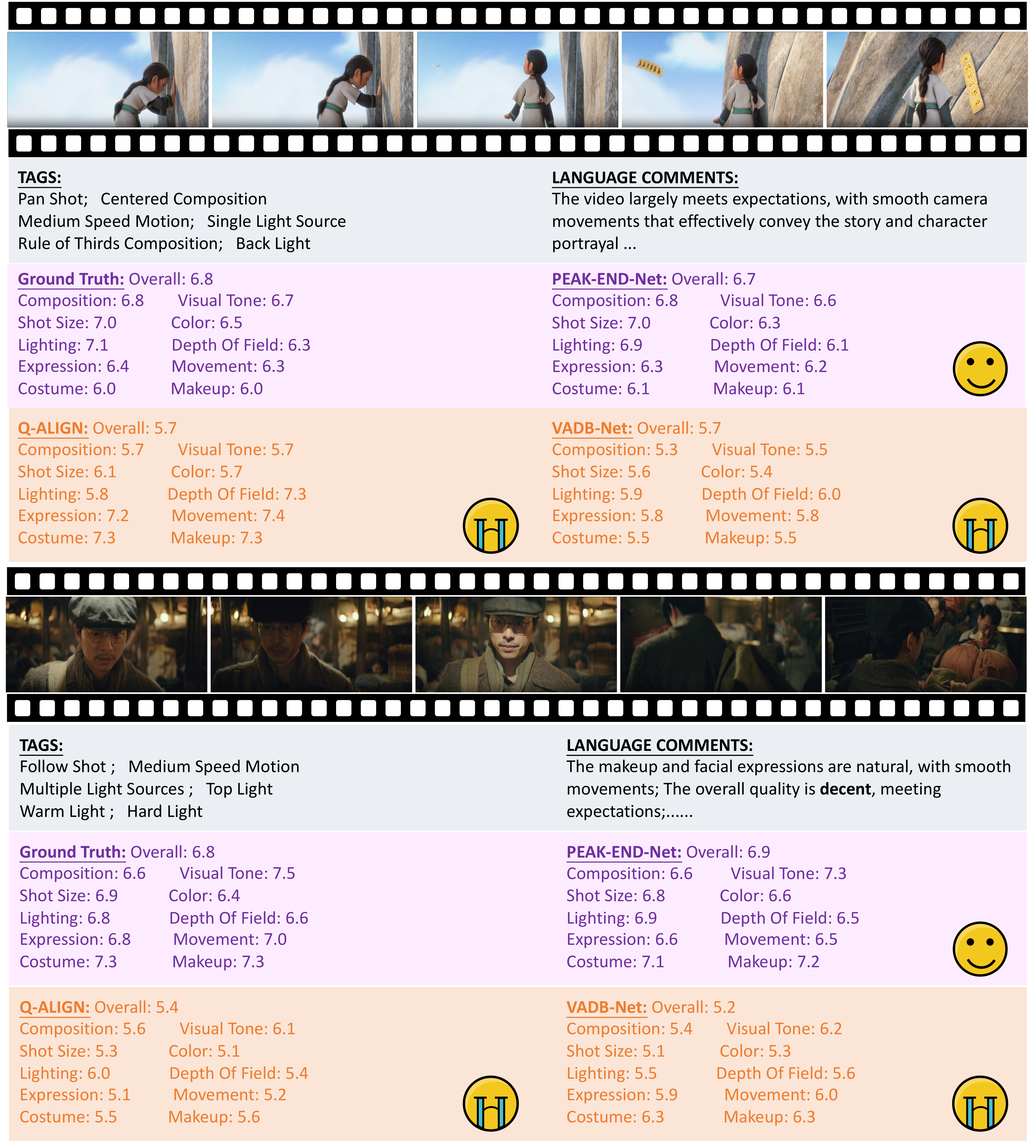
Figure 3 presents two representative examples from VADB. In both cases, Peak-End-Net produces predictions that are much closer to the ground truth than Q-Align and VADB-Net, not only on the overall score but also across fine-grained attribute dimensions. In the first example, Peak-End-Net accurately captures the balanced aesthetic quality reflected in composition, shot size, and lighting, while the other two methods exhibit obvious deviations. In the second example, Peak-End-Net again better matches the ground-truth annotations, especially on visual tone, movement, costume, and makeup. These cases suggest that Peak-End-Net is able to provide more reliable and consistent multi-dimensional aesthetic predictions.
4.4 Ablation Study↩︎
Effectiveness of Peak-End Aggregation. Table ¿tbl:tab:method95comparison? reports the ablation results on the Overall dimension of VADB. Comparison with alternative temporal aggregation strategies. We compare the proposed peak-end aggregation with mean pooling, max pooling, and a temporal transformer, where the latter introduces a learnable temporal module for feature aggregation (details in the Appendix). Peak-end aggregation outperforms all alternatives, improving RMSE from 0.4654 to 0.4548 and SRCC from 0.8683 to 0.8804 over the temporal transformer baseline. This shows that explicitly textitasizing salient moments and the ending segment is more effective than generic temporal aggregation for video aesthetic assessment. Effectiveness of the pretrained IAA head and rhythm encoder. Replacing the randomly initialized IAA head \(\Phi_\text{IAA}^{\text{random}}\) with the AVA-pretrained \(\Phi_\text{IAA}\) consistently improves all four metrics, verifying the benefit of transferring image-aesthetic priors. Adding the rhythm encoder \(\Phi_\text{RE}\) brings additional gains, leading to the best overall performance. This suggests that, in addition to emphasizing salient moments and the ending effect, modeling aesthetic progression is also beneficial for VAA.
Components in Peak-End Aggregation. Table 3 presents the ablation study of different components in the proposed peak-end rule-based aggregation. To reduce the interference of other modules, we conduct the ablation study based on Peak-End + \(\Phi_\text{random}\) in Table ¿tbl:tab:method95comparison?. Single-component variants. Using only one component, i.e., Peak, End, or Valley, yields limited performance, indicating that no single temporal cue is sufficient to capture holistic video aesthetics. Among them, the End-only variant shows slightly better overall behavior, suggesting that recency information is an important factor in aesthetic judgment. Two-component variants. Combining any two components generally leads to better results than using a single one, which suggests that these temporal cues are complementary and exhibit a certain degree of collaboration. This confirms that VAA benefits from integrating multiple temporal factors rather than relying on an isolated cue. Full peak-end aggregation. The full model that jointly incorporates Peak, End, and Valley achieves the best performance among all variants. This verifies that a more complete temporal representation, covering salient moments, ending effects, and unfavorable valleys, is most effective for VAA.
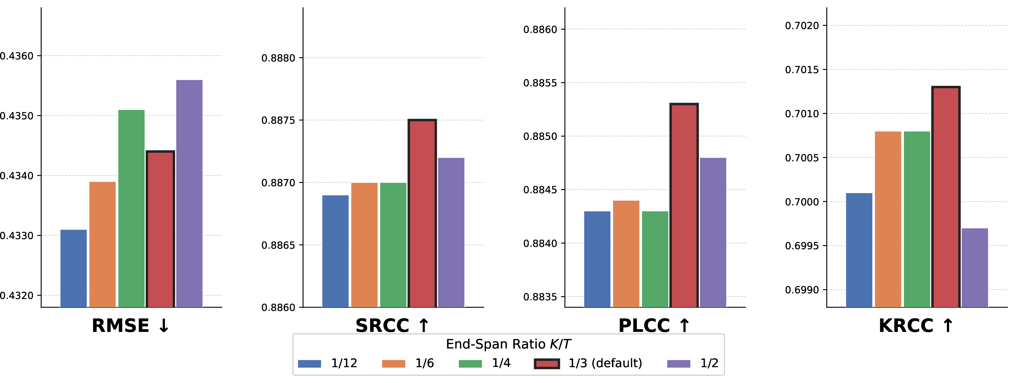
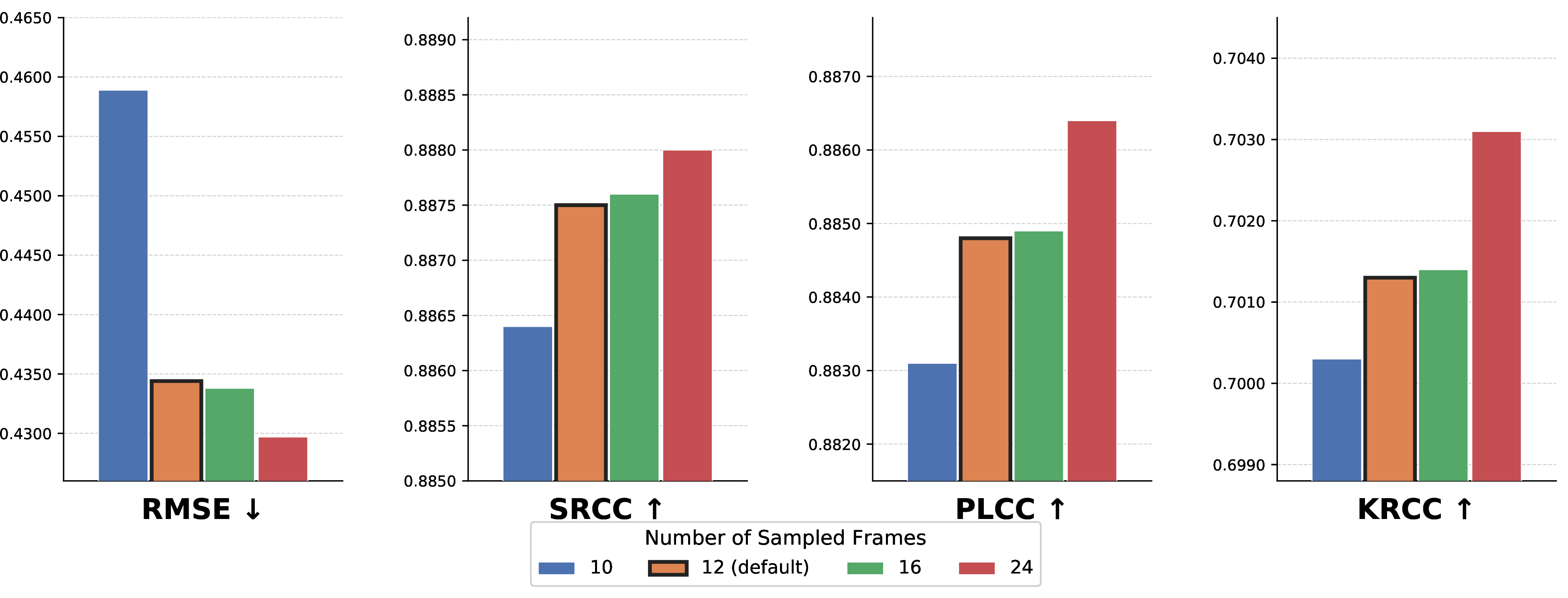
Figure 4: Sensitivity analysis of key hyperparameters..
Sensitivity Analysis of Key Hyperparameters. Figure 4 analyzes two key hyperparameters. Effect of the end-span ratio \(K/T\). With 12 sampled frames, using the last one-third of the video (\(K=4\)) gives the best performance, showing the importance of properly modeling the ending segment. Effect of the number of sampled frames. Performance generally improves with more sampled frames, suggesting that denser temporal observation is beneficial. To balance accuracy and efficiency, we adopt 12 frames by default.
| Dataset | Variant | SRCC\(\uparrow\) | PLCC\(\uparrow\) | KRCC\(\uparrow\) |
|---|---|---|---|---|
| Peak-End-Net (Stage 1) | 0.4600 | 0.4832 | 0.3009 | |
| + Static Average Fusion | 0.5285 (+0.0685) | 0.5746 (+0.0914) | 0.3860 (+0.0851) | |
| + Learnable Scalar Fusion | 0.5248 (+0.0648) | 0.5588 (+0.0756) | 0.3701 (+0.0692) | |
| + Dynamic Gated Fusion (Ours) | 0.5427 (+0.0827) | 0.5773 (+0.0941) | 0.3745 (+0.0736) | |
| Peak-End-Net (Stage 1) | 0.8875 | 0.8853 | 0.7014 | |
| + Static Average Fusion | 0.8353 (-0.0522) | 0.8391 (-0.0462) | 0.6334 (-0.0679) | |
| + Learnable Scalar Fusion | 0.8691 (-0.0184) | 0.8690 (-0.0163) | 0.6780 (-0.0233) | |
| + Dynamic Gated Fusion (Ours) | 0.8784 (-0.0091) | 0.8765 (-0.0088) | 0.6925 (-0.0089) |
Effectiveness of Dynamic Gated Fusion. Table 4 reports the comparison of different Stage 2 fusion strategies on both VADB and DIVIDE-3K. In this part, we further compare our method with two fusion baselines. Static Average Fusion directly averages the Stage 1 overall prediction and the global IAA score with equal weights. Learnable Scalar Fusion replaces the fixed averaging weight with a single learnable scalar shared by all samples. All fusion variants improve the cross-dataset performance on DIVIDE-3K over Stage 1, indicating that the global IAA estimate provides meaningful transferable information. Static Average Fusion achieves the largest gain in KRCC, while the proposed Dynamic Gated Fusion achieves the largest gains in SRCC and PLCC.
The key difference lies in their impact on the source-domain VADB test set. Static Average Fusion obtains cross-dataset gains at the cost of a substantial degradation on VADB, with clear drops in all three metrics. This suggests that its improvement mainly comes from sacrificing source-domain performance. Learnable Scalar Fusion alleviates this issue to some extent, but still causes noticeable performance loss. In contrast, our dynamic gated fusion improves the cross-dataset performance while introducing only very small decreases on VADB. Therefore, our proposed method achieves a much more favorable trade-off between cross-dataset robustness and in-domain prediction quality.
5 Discussion↩︎
We provide a brief discussion: Beyond benchmark evaluation, our model can be used for large-scale video aesthetic filtering and as a reward model for RL-based video generation or editing. Compared with LLM-based approaches, our method is more efficient and can be naturally scaled to arbitrary aesthetic dimensions by adjusting the prediction heads. In contrast, although LLM-based methods offer better verbal interpretability, they show no clear performance advantage in our experiments and are less suitable for multi-dimensional scoring due to higher inference costs. Our method is built on the peak-end rule with a relatively minimal design. While the current architecture may not be optimal, it demonstrates that psychologically grounded temporal aggregation is highly valuable for VAA. Our key contribution lies in the underlying idea.
6 Conclusion↩︎
In this paper, we presented Peak-End-Net, a psychologically grounded framework for video aesthetic assessment inspired by the peak-end rule. By leveraging frame-wise aesthetic priors from a pretrained IAA head, our method transfers image-level aesthetic knowledge to video-level modeling without requiring frame-level video annotations. Complemented by an aesthetic rhythm encoder that captures temporal progression and a dynamic gated fusion mechanism that adaptively integrates image-aesthetic priors for robust overall-score prediction, Peak-End-Net achieves state-of-the-art performance on both settings: in-domain evaluation on VADB and zero-shot transfer to DIVIDE-3K. Extensive ablation studies further validate the contribution of each component and confirm the robustness of the proposed design. We hope this work encourages future research to explore psychologically grounded modeling principles for perceptual video understanding.
This appendix mainly includes a detailed introduction to the benchmarks involved in the main paper (Sec. 7), the specific implementations of the proposed modules (Sec. 8), computational efficiency analysis (Sec. 9), and additional visualizations (Sec. 10).
7 Benchmark Details↩︎
Video Aesthetic Database (VADB) [1] is a large-scale dataset for video aesthetic assessment (VAA). It was proposed to address the lack of standardized and richly annotated benchmarks in this area. The dataset contains 10,490 videos collected from diverse sources, including films, TV dramas, documentaries, news, user-generated content, and AI-generated videos. A small portion of the videos has not yet been publicly released due to copyright restrictions. Each clip is 5–20 seconds long and belongs to one of four categories: character, natural scenery, architecture, and food.
A major feature of VADB is its professional and multi-dimensional annotation scheme. The dataset was annotated by 37 trained professionals with backgrounds in film, television, and media studies, under a carefully designed aesthetic framework developed by experts from the Beijing Film Academy. Each video has annotations from at least 13 annotators, including aesthetic scores, language comments, and technical tags. VADB provides an overall aesthetic score as well as attribute-level scores. The annotated attributes include composition, shot size, lighting, visual tone, color, depth of field, expression, movement, costume, and makeup. It also includes objective tags related to camera movement, composition, and lighting. Representative samples are shown in Figure 5 (Top).
Compared with previous video aesthetic datasets, VADB is larger and more comprehensive in both scale and annotation richness. By combining numerical scores, textual comments, and technical tags, it offers a valuable benchmark for research on fine-grained video aesthetic assessment.
Disentangled Video Quality Database (DIVIDE-3K) [2] is a large-scale user-generated content video quality assessment (UGC-VQA) database proposed to study video quality from both technical and aesthetic perspectives. Unlike previous UGC-VQA datasets that usually provide only one overall quality score, DIVIDE-3K explicitly disentangles how people judge videos in terms of visual distortions and content preference. The dataset contains 3,590 real-world videos collected mainly from YFCC-100M [51] and Kinetics-400 [52], covering diverse scenes, content, and quality levels. To ensure reliable annotations, the authors conducted an in-lab subjective study with 35 trained annotators, rather than relying on crowdsourcing. In total, the dataset includes about 450,000 human opinions, including overall quality scores, aesthetic scores, technical scores, and additional subjective reasoning labels that indicate how much each perspective influences the final overall judgment.
A key finding enabled by DIVIDE-3K is that human perception of UGC video quality is almost always shaped by both perspectives: a technically clean video may still be rated poorly if its content is unappealing, while an aesthetically attractive video may receive favorable scores despite distortions. Therefore, DIVIDE-3K provides a more comprehensive benchmark for understanding human quality perception and for developing explainable VQA models, such as DOVER, that can predict both overall quality and perspective-specific quality. Two samples are shown in Figure 5.
![Figure 5: Some representative samples: the two above are from VADB [1], and in our experiments we only used the scores; the two below are from DIVIDE-3K [2], and we only evaluated the aesthetic dimension, i.e., the Aesthetic Score.](/article/2607.13941/files/vadb_divide.png "fig:")
8 Detailed Architectures↩︎
The visual backbone we use is ViT-L/14 [16], initialized with CLIP [17] pretrained weights, whose output frame-level visual features are denoted as \(\mathbf{F}_v=\{\mathbf{f}_t \in \mathbb{R}^d\}_{t=1}^T\), where \(T=12\) by default and \(d=768\).
8.1 IAA Head \(\Phi_{\text{IAA}}\)↩︎
The IAA head \(\Phi_{\text{IAA}}\) is pretrained on the AVA [15] dataset and then kept frozen and applied to the frame-level
visual features. Given \(\mathbf{f}_t\in\mathbb{R}^{768}\), the head predicts a 10-dimensional logit vector: \[\mathbf{z}_t=\Phi_{\text{IAA}}(\mathbf{f}_t)\in\mathbb{R}^{10}.\] \(\Phi_{\text{IAA}}\) is implemented as an MLP with dimensions 768 \(\rightarrow\) 512 \(\rightarrow\) 10, where the first
hidden layer is followed by LayerNorm, ReLU, and Dropout, and the second hidden layer is followed by ReLU and Dropout. The dropout ratio is \(0.3\). The
logits are normalized by softmax to obtain a 10-way aesthetic distribution, which is used to compute a weighted aesthetic score \(s_t\) for each sampled frame.
8.2 Rhythm Encoder \(\Phi_{\text{RE}}\)↩︎
The rhythm encoder \(\Phi_{\text{RE}}\) models temporal variation patterns in the frame-wise aesthetic score sequence \(\mathbf{s}=[s_1,\dots,s_T]\in\mathbb{R}^{1\times T}\). It treats
\(\mathbf{s}\) as a 1D temporal signal and applies three parallel 1D convolution branches with kernel sizes 3, 5, and 7, respectively. Each branch has channel dimensions \(\texttt{1} \rightarrow
\texttt{16} \rightarrow \texttt{32}\) with GELU activations. The three outputs are concatenated into a \(96\times T\) feature map and fused by a \(1\times1\) convolution
into a \(64\times T\) representation. After Mean-pooling over time, a linear Projection and LayerNorm are applied to obtain the final rhythm feature (\(d'=64\)): \[\mathbf{f}_{\text{rhythm}}=\Phi_{\text{RE}}(\mathbf{s})\in\mathbb{R}^{d'}.\]

8.3 VAA Head \(\Phi_{\text{VAA}}\)↩︎
The VAA head \(\Phi_{\text{VAA}}\) predicts the overall and attribute-level scores from the concatenated representation: \[\mathbf{f}_{\text{concat}}=\mathbf{f}_{\text{video}}\oplus\mathbf{f}_{\text{rhythm}}.\] It consists of a shared MLP backbone with dimensions \((\texttt{768+64}) \rightarrow \texttt{512} \rightarrow
\texttt{256}\), followed by LayerNorm, where GELU activations are used after each layer and dropout with ratio \(0.1\) is applied after the first layer. Based on the shared
feature, we use \(11\) attribute-specific regression heads, each implemented as \(\texttt{256} \rightarrow \texttt{128} \rightarrow \texttt{1}\). The outputs of all heads are concatenated
into an 11-dimensional vector, followed by a sigmoid function to obtain normalized scores, which are used to compute \(\mathcal{L}_\text{VAA}\).
8.4 Gate Fusion Module \(\Phi_{\text{GF}}\)↩︎
The gate fusion module \(\Phi_{\text{GF}}\) predicts a sample-wise scalar gate \(\lambda\) for combining the predicted VAA overall score and the global IAA score. It takes \(\mathbf{f}_{\text{video}}\oplus\mathbf{f}_{\text{rhythm}}\) as input and is implemented as a two-layer MLP with dimensions \((\texttt{768+64}) \rightarrow \texttt{128} \rightarrow \texttt{1}\),
followed by GELU, Dropout (\(p=0.1\)), and a final sigmoid activation. The fused overall score is computed as: \[\hat{y}^{\,\text{fusion}}_{\text{overall}}
=
\lambda\,\hat{y}_{\text{overall}}
+
(1-\lambda)\,\hat{y}_{\text{IAA}},\] where \(\lambda\in[0,1]\) is the predicted gate value.
8.5 Temporal Transformer Baseline↩︎
For the temporal transformer baseline in Table 4 of the main paper, we replace the proposed peak-end aggregation with a standard transformer-based temporal encoder over frame-level features. A learnable token is prepended to the frame sequence,
and learnable temporal positional embeddings are added before the tokens are fed into the encoder. The model uses \(4\) transformer encoder layers, \(8\) attention heads, hidden dimension
\(768\), and a feed-forward dimension \(2048\), with LayerNorm and Dropout (\(p=0.1\)). The video representation is taken as the
output of the token.
9 Computational Efficiency↩︎
Another advantage of our framework is its parameter-efficient training scheme. Compared with VADB-Net [1], which involves training the visual and textual backbones, and Q-Align [45], which adapts a much larger multimodal large language model [53], our method keeps the ViT backbone frozen and uses a frozen AVA-pretrained IAA head. Only lightweight modules, including \(\Phi_{\text{VAA}}\), \(\Phi_{\text{RE}}\), and \(\Phi_{\text{GF}}\) are optimized during training.
Specifically, the total number of trainable parameters in our method is only 1.05M, accounting for less than 1% of the total parameter count. The number of trainable parameters is much smaller than that of VADB-Net and Q-Align, leading to lower training cost and memory demand while achieving stronger performance.
10 Additional Qualitative Results↩︎
Figure 6 presents additional qualitative examples on VADB. Advantage of Peak-End-Net. In most cases, Peak-End-Net produces predictions that are noticeably closer to the ground truth than Q-Align [45] and VADB-Net [1], especially for videos with large frame-wise variation. When the visual quality changes significantly across time, our method can better capture the contribution of salient moments and the ending segment, leading to more accurate overall and attribute-level assessment. This suggests that explicitly modeling temporal aesthetic dynamics is important for video aesthetic assessment. Failure cases and possible reasons. We also observe several failure cases where Peak-End-Net loses its advantage or produces less accurate predictions. A possible reason is that some videos contain subtle aesthetic cues that are difficult to infer from sparsely sampled frames alone, such as fine-grained semantic intent, narrative coherence, or subjective preference. In addition, when the visual quality is relatively uniform, the benefit of our temporal modeling may become less evident.