Partially Correlated Verifier Cascades in LLM Harnesses:
Concave Log-Odds, Polynomial Reliability, and Blind-Spot Ceilings
July 15, 2026
Abstract
Serial verification gates are a core reliability primitive in LLM harnesses: a candidate answer is returned only if \(k\) verifier calls all accept it. Under conditionally independent gates, the recent Odds Law [1] shows that posterior log-odds grow linearly in \(k\), so failure decays exponentially; the same work states that “a tight theory of partially correlated verifier cascades remains open.” This note gives a minimal such theory. It carries the latent-variable/moment machinery developed for correlated voting [2], [3] over to the structurally different conjunctive verification primitive, where a survivorship effect with no one-shot-voting analogue — errors that survive \(j\) gates are exactly the high-\(\alpha\) ones — is the mechanism behind the concavity, the ceiling, and the trichotomy below. Modeling the per-instance false-accept rate of the verifier on the generator’s own errors as a latent variable \(\alpha\sim G\) (de Finetti), the exact cascade posterior is \(\ell_k=\ell_0-\ln m_k\), with \(m_k\) the \(k\)-th moment of \(G\), and: (i) \(\ell_k\) is concave in \(k\) for every non-degenerate \(G\) — the Odds Law is its tangent at the first gate and an upper bound; (ii) for \(\mathrm{Beta}(a,b)\) latents, failure decays polynomially, \(1-r_k\asymp k^{-b}\), not exponentially, with all formulas governed by a single correlation parameter \(\rho_v=1/(a+b+1)\); (iii) a blind-spot atom of mass \(1-\pi\) at \(\alpha=1\) caps the total evidence extractable from any number of gates at \(-\ln(1-\pi)\) nats, so reliability saturates strictly below \(1\); (iv) letting the true-accept rate also vary across instances (\(\beta\sim H\)) yields a trichotomy — gates eventually always help, plateau, or actively harm — decided by the upper-tail exponents \(b_\alpha\) vs.\(b_\beta\) of \(G\) and \(H\), with closed-form crossover \(k^\dagger=\frac{a_\alpha b_\beta-a_\beta b_\alpha}{b_\alpha-b_\beta}\); mean gate quality \(\bar\Lambda>1\) no longer guarantees that gating helps. Because everything is a functional of \(G\), the theory is measurable: \(R\) repeated verdicts per instance identify the first \(R\) moments of \(G\), so two verdicts identify \(\rho_v\); beta-binomial likelihood and NPMLE recover the full reliability curve and the (tail-dominated, ill-posed) ceiling. Synthetic-recovery experiments validate the estimators and the falsification loop: independence-based extrapolation underestimates the failure rate by \(20\times\) at \(k=5\) and \(\approx3000\times\) at \(k=10\) in a realistic regime, while the correlated theory fitted at order \(R=8\) tracks held-out depths. The practical lever the theory isolates is decorrelation — changing model family, modality, or evidence source — rather than adding gates.
1 Introduction↩︎
An LLM harness improves the reliability of an unreliable base model by composing calls: decompose, ensemble, verify, recurse. The lineage of this program is von Neumann’s synthesis of reliable organisms from unreliable components [4], and its most recent and most explicit algebraic form is the Odds Law of [1], with a companion orchestration harness [5]. For the verification primitive — pass a candidate answer through \(k\) accept/reject gates and return it only if all accept — the Odds Law is sharp and simple: writing \(\ell=\ln\frac{P(\text{correct})}{P(\text{wrong})}\) for log-odds and \(\Lambda=\beta/\alpha\) for a gate’s likelihood ratio (true-accept over false-accept rate), conditionally independent gates each add a fixed evidence increment, \[\label{eq:oddslaw} \ell_k=\ell_0+k\ln\Lambda ,\tag{1}\] so reliability \(r_k=\sigma(\ell_k)\) (\(\sigma\) the logistic function) approaches \(1\) exponentially fast, and \(k=O\!\big(\tfrac{\log(1/\delta)}{\log\Lambda}\big)\) gates suffice for reliability \(1-\delta\) [1]. The same framework contains a threshold dichotomy at \(\Lambda^\star=1\) [1] and a correlation-aware theory of the voting primitive via a latent-factor model [1].
The assumption doing the work in 1 is conditional independence of gate errors. It fails in the situation harnesses actually face: verifiers built from the same model family, prompt style, or training distribution as the generator share blind spots with it — error types the generator likes to produce and the verifier reliably fails to catch. Empirically such blind spots are large: across 14 open models, an average \(64.5\%\) of self-generated errors survive self-checking even though the same errors are caught when presented externally [6]. The broader self-correction literature reaches the same verdict: prompted-LLM self-feedback rarely repairs reasoning errors and can even degrade accuracy, and reliable improvement generally requires external feedback rather than more of the same model [7], [8]. [1] are explicit that this is the open boundary of their algebra: “a tight theory of partially correlated verifier cascades remains open.”
This note supplies a minimal such theory, together with a protocol for measuring the correlation it introduces. Methodologically, the latent-variable/moment identification we use is the verification-side counterpart of the two-call framework recently developed for correlated voting [2], [3]; what is specific to conjunctive verification — the survivorship tilt, and the phenomena it produces (concave depth-scaling, blind-spot ceiling, two-sided trichotomy, a zero-cost internal optimum) — has no one-shot-voting analogue and is the new content here. Our contributions:
Exact cascade posterior and concavification (§3). Treating the per-instance false-accept rate as a latent variable \(\alpha\sim G\) — exchangeability across gates plus de Finetti — gives the exact posterior \(\ell_k=\ell_0-\ln m_k\) with \(m_k=\mathbb{E}[\alpha^k]\). Since \(\ln m_k\) is a cumulant generating function, \(\ell_k\) is concave in \(k\) for every non-degenerate \(G\): the Odds Law is the degenerate (\(\rho_v\to0\)) case, coincides with the true curve only at the first gate, and upper-bounds it everywhere else. The mechanism is a survivorship effect specific to verification: errors that survive \(j\) gates are exactly the high-\(\alpha\) ones, so late gates face selected survivors.
Polynomial reliability and a one-parameter family (§3). For \(G=\mathrm{Beta}(a,b)\), \(1-r_k\sim\kappa\,k^{-b}\): correlation degrades the exponential convergence of 1 to polynomial. The single parameter \(\rho_v=\mathop{\mathrm{Var}}(\alpha)/(\bar\alpha(1-\bar\alpha))=1/(a+b+1)\) — the within-instance correlation of two verdicts — interpolates continuously from the Odds Law (\(\rho_v\to0\)) to a pure blind-spot model (\(\rho_v\to1\)). The cost-optimal gate count becomes a power of the value/cost ratio instead of its logarithm.
Blind-spot ceiling (§3). An atom of mass \(1-\pi\) at \(\alpha=1\) (errors the verifier never catches) caps the total extractable evidence of the entire cascade at \(-\ln(1-\pi)\) nats: \(r_\infty=p_0/(p_0+(1-p_0)(1-\pi))<1\) no matter how many gates. This is the verification-side dual of the correlated-voting floor ([1] Thm. 7.2; [9]).
Two-sided trichotomy with closed-form crossover (§4). If the true-accept rate also varies across instances (\(\beta\sim H\)), then \(\ell_k=\ell_0+\ln m_k^{(\beta)}-\ln m_k^{(\alpha)}\) and asymptotically \(\ell_k\approx\mathrm{const}+(b_\alpha-b_\beta)\ln k\): gates eventually always help, plateau, or actively harm according to whether the upper-tail exponent of \(G\) exceeds, equals, or falls below that of \(H\). In the harmful regime the reliability peaks at a closed-form crossover \(k^\dagger=\frac{a_\alpha b_\beta-a_\beta b_\alpha}{b_\alpha-b_\beta}\) and then decays to zero — even when the mean likelihood ratio satisfies \(\bar\Lambda>1\), so the independence-based dichotomy at \(\Lambda^\star=1\) is no longer the right criterion under correlation.
Identification and inversion of \(\rho_v\) (§5–6). All of the above are functionals of \(G\), and \(G\) is estimable from accept/reject logs alone: with \(R\) repeated verdicts per instance on the generator’s own errors, \(X_i\sim\mathrm{Bin}(R,\alpha_i)\), unbiased U-statistics identify moments up to order \(R\) — so \(R=2\) already identifies \(\rho_v\). Beta-binomial likelihood recovers the reliability curve; nonparametric MLE recovers atoms. We quantify the intrinsic ill-posedness of the ceiling (an upper-tail functional, boundary resolution \(\sim1/R\)) and validate the full pipeline in synthetic-recovery experiments, including the falsification loop: fit at low order, predict held-out gate depths.
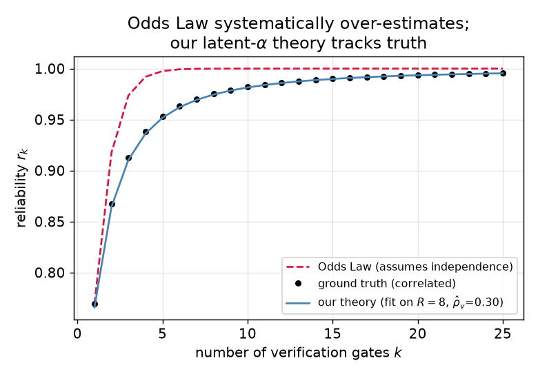
In one sentence, the correction this note makes to the Odds Law: correlation does not tax the first gate; it taxes the extrapolation. And the practical lever it isolates: once \(\rho_v\) is large, adding gates buys almost nothing — reliability is bought by decorrelating the verifier from the generator (different model family, different modality, external oracles, tool-based checks), which raises \(b\), shrinks the blind-spot mass, and lifts the ceiling.
2 Setup↩︎
2.0.0.1 Gates and survivor reliability.
A candidate answer has truth label \(C\in\{1,0\}\) with prior \(p_0=\mathbb{P}(C{=}1)\), prior odds \(o_0=p_0/(1-p_0)\), \(\ell_0=\ln o_0\). It is passed through \(k\) verification gates under all-accept (conjunctive) gating: the answer is returned only if all \(k\) gates accept. A gate has true-accept rate \(\beta=\mathbb{P}(\text{accept}\mid C{=}1)\) and false-accept rate \(\alpha=\mathbb{P}(\text{accept}\mid C{=}0,\text{instance})\). We study the survivor reliability \[r_k \;=\; \mathbb{P}\big(C{=}1 \,\big|\, \text{all }k\text{ gates accept}\big),\] the precision of what the cascade returns. In the generate–verify–retry loop that real harnesses run (regenerate until some candidate passes), the returned answer is by construction a survivor, so \(r_k\) is the end-to-end correctness of what the harness emits; rejected correct answers cost throughput, not precision. Section 3 sets \(\beta\equiv1\) (no false rejections) as an explicit idealization; §4 removes it.
2.0.0.2 Latent false-accept rate and the generator–verifier bridge.
The central modeling step: \(\alpha\) is not a constant of the verifier but a property of the instance, distributed across instances as \[\alpha\sim G \quad\text{supported on }[0,1],\] where the instance population is the generator’s own erroneous outputs. This bridge matters. \(G\)’s upper tail — mass near \(\alpha=1\) — is precisely the set of errors the generator likes to make and the verifier fails to catch: the generator–verifier blind-spot alignment. A verifier can be excellent on random errors and still have a heavy \(G\)-tail on its own generator’s errors [6]; empirically this tail thickens as the generator strengthens — stronger generators produce errors that are systematically harder to detect [10]. Consequently (§5) any measurement of \(G\) must use the generator’s own errors as the test population, not synthetic or third-party errors.
Assumption 1 (de Finetti idealization). Given the instance (i.e., given \(\alpha\)), the \(k\) gate verdicts are i.i.d.\(\mathrm{Bernoulli}(\alpha)\) on an erroneous answer (resp.\(\mathrm{Bernoulli}(\beta)\) on a correct one).
This is exact for exchangeable verdicts by de Finetti’s theorem, and covers the two operational readings of “\(k\) gates”: \(k\) samples of the same verifier at temperature \(>0\) (then \(\alpha\) is that verifier’s per-instance acceptance propensity), or \(k\) verifiers from a family sharing blind spots (then \(\alpha\) is the family-level propensity). It is a mean-field idealization in the same spirit as von Neumann’s constant component-failure probability [4]: all shared structure between gates is compressed into a scalar latent, residual gate-specific correlations are ignored. Everything below is a first-order theory in this sense, and we flag it as the main relaxable assumption.
3 One-sided theory: concavity, polynomial decay, ceiling↩︎
Throughout this section \(\beta\equiv1\). Write \(m_k=\mathbb{E}_{\alpha\sim G}[\alpha^k]\) for the \(k\)-th moment of \(G\), and \(\bar\alpha=m_1\).
Proposition 1 (Exact cascade posterior). Under Assumption 1, \[\label{eq:exact} \ell_k=\ell_0-\ln m_k, \qquad r_k=\frac{p_0}{p_0+(1-p_0)\,m_k},\qquad{(1)}\] and \(r_k\) is nondecreasing in \(k\).
Proof. Given \(C{=}1\), all gates accept with probability \(1\). Given \(C{=}0\), the instance carries \(\alpha\sim G\) and, conditionally, all \(k\) accept with probability \(\alpha^k\); marginally \(\mathbb{P}(\text{all accept}\mid C{=}0)=\mathbb{E}[\alpha^k]=m_k\). Bayes in odds form gives \(o_k=o_0/m_k\); take logs and invert. Monotonicity: \(m_k\) is nonincreasing since \(\alpha\le1\). ◻
Corollary 1 (Odds Law as the degenerate case). If \(G=\delta_{\bar\alpha}\) (no correlation), \(m_k=\bar\alpha^{\,k}\) and ?? reduces to \(\ell_k=\ell_0+k\ln\Lambda\) with \(\Lambda=1/\bar\alpha\): exactly 1 .
Theorem 2 (Concavification). For any \(G\), \(k\mapsto\ell_k\) is concave on \(k\ge0\); strictly concave unless \(G\) is degenerate. Moreover the per-gate evidence increments \[\Delta_{j+1}:=\ell_{j+1}-\ell_j=\ln\frac{m_j}{m_{j+1}}=-\ln \mathbb{E}_{(j)}[\alpha], \qquad d G_{(j)}\propto \alpha^{j}\,dG,\] are strictly decreasing, with \(\mathbb{E}_{(j)}[\alpha]\uparrow\mathop{\mathrm{ess\,sup}}\alpha\). Consequently the Odds Law line through the first gate, \(\ell_0+k\Delta_1\), upper-bounds \(\ell_k\) for all \(k\ge1\), with equality only at \(k\in\{0,1\}\).
Proof. \(\ln m_k=\ln\mathbb{E}[e^{k\ln\alpha}]\) is the cumulant generating function of \(\ln\alpha\) evaluated at \(k\), hence convex (strictly, unless \(\ln\alpha\) is a.s.constant); \(\ell_k=\ell_0-\ln m_k\) is concave. The increment identity is algebra; \(G_{(j)}\) is the \(\alpha^j\)-tilted (size-biased) distribution, which concentrates on the essential supremum as \(j\to\infty\), so \(\Delta_{j+1}\downarrow -\ln\mathop{\mathrm{ess\,sup}}\alpha\) (zero when \(\mathop{\mathrm{ess\,sup}}\alpha=1\)). The tangent bound is concavity. ◻
Remark 3 (Survivorship mechanism). The tilt \(dG_{(j)}\propto\alpha^j dG\) is the population of errors still alive after \(j\) gates: surviving errors are precisely the ones selected for fooling the verifier. Late gates face survivors, not fresh errors — which is why their evidence decays to zero. This selection effect is specific to conjunctive verification; it has no analogue in one-shot voting, where all votes face the same instance.
Theorem 4 (Exponential \(\to\) polynomial). Suppose \(G\) has no atom at \(1\) and density \(g(\alpha)\sim c\,(1-\alpha)^{b-1}\) as \(\alpha\uparrow1\) for some \(b,c>0\). Then \[m_k\;\sim\; c\,\Gamma(b)\,k^{-b}, \qquad 1-r_k\;\sim\;\kappa\,k^{-b}, \qquad \kappa=\tfrac{1-p_0}{p_0}\,c\,\Gamma(b).\] In particular for \(G=\mathrm{Beta}(a,b)\): \(m_k=\frac{(a)_k}{(a+b)_k}=\prod_{j=0}^{k-1}\frac{a+j}{a+b+j}\) exactly, and \(c\,\Gamma(b)=\frac{\Gamma(a+b)}{\Gamma(a)}\).
Proof in Appendix 9.1. The contrast with 1 is the headline: under independence \(1-r_k\sim\frac{1-p_0}{p_0}\bar\alpha^{\,k}\) decays exponentially; any latent heterogeneity with a regularly-varying upper tail degrades this to polynomial \(k^{-b}\), where \(b\) measures how thin the blind-spot tail is. Only the tail exponent matters asymptotically; the Beta family adds exact finite-\(k\) formulas.
Theorem 5 (Blind-spot ceiling). Let \(G=\pi\,\mathrm{Beta}(a,b)+(1-\pi)\,\delta_1\) with blind-spot mass \(1-\pi\in(0,1)\). Then \(m_k\downarrow 1-\pi\) and \[\sup_k\,(\ell_k-\ell_0)=-\ln(1-\pi), \qquad r_\infty=\frac{p_0}{p_0+(1-p_0)(1-\pi)}<1 .\]
Proof. \(m_k=\pi\,m_k^{\mathrm{Beta}}+(1-\pi)\to1-\pi\) by Theorem 4; plug into ?? . ◻
The entire cascade — any number of gates from the same correlated family — carries a finite evidence budget of \(-\ln(1-\pi)\) nats, set by the blind-spot mass alone, not by \(\Lambda\) or \(k\). This is the verification-side dual of the correlated-voting floor (\(n_{\mathrm{eff}}=1/\gamma\), majority-error floor \(\mathbb{P}[p(S)<1/2]\)) of [1] and, classically, of correlated-jury theorems [9]. On the voting side this ceiling is by now also an empirical fact: a panel of nine frontier judges from seven model families supplies only about two independent votes’ worth of information, and neither more judges nor smarter aggregation closes the gap [11].
Proposition 6 (One correlation parameter). For two gate verdicts \(\mathbf{1}_1,\mathbf{1}_2\) on an erroneous instance, \[\rho_v:=\mathrm{Corr}(\mathbf{1}_1,\mathbf{1}_2)=\frac{\mathop{\mathrm{Var}}(\alpha)}{\bar\alpha(1-\bar\alpha)} \;\overset{\mathrm{Beta}(a,b)}{=}\;\frac{1}{a+b+1}.\] \(\rho_v\to0\) (with \(\bar\alpha\) fixed) recovers the Odds Law; \(\rho_v\to1\) recovers a two-point blind-spot model (\(\alpha\in\{0,1\}\)), where gates either succeed immediately or never.
Proof. \(\mathbb{E}[\mathbf{1}_1\mathbf{1}_2]=\mathbb{E}[\alpha^2]=m_2\), \(\mathbb{E}[\mathbf{1}_i]=\bar\alpha\), so \(\mathop{\mathrm{Cov}}=m_2-\bar\alpha^2=\mathop{\mathrm{Var}}(\alpha)\) and \(\mathop{\mathrm{Var}}(\mathbf{1}_i)=\bar\alpha(1-\bar\alpha)\). For Beta, \(\mathop{\mathrm{Var}}(\alpha)=\frac{ab}{(a+b)^2(a+b+1)}\). ◻
\(\rho_v\) is the same intraclass-correlation functional that governs the voting side [1], [9], now appearing on the verification side, and — unlike a modeling parameter — it is directly measurable (§5).
Corollary 2 (Cost-optimal gate count). With per-gate cost \(c\), success value \(U\), and objective \(J(k)=U r_k-ck\), the optimum under Theorem 4 scales as \[k^{*}\approx\Big(\frac{U\kappa b}{c}\Big)^{\!1/(b+1)} \quad\text{(power law)}, \qquad\text{vs.}\qquad k^{*}_{\mathrm{indep}}\sim\frac{\ln(U/c)}{\ln(1/\bar\alpha)} \quad\text{(logarithmic)}.\]
Proof in Appendix 9.2. Correlation is a double penalty: each gate buys less, and reaching a target reliability requires polynomially rather than logarithmically many gates — until the ceiling makes the target unreachable altogether.
3.0.0.1 How large is the error of assuming independence?
Table 1 evaluates ?? in a moderate regime: \(p_0=0.5\), \(\bar\alpha=0.3\) (a decent verifier: catches \(70\%\) of errors per gate), \(\rho_v=0.3\) (\(a=0.7\), \(b\approx1.63\)), against the Odds Law with the same \(\bar\alpha\). The curves agree at \(k=1\) by construction and then split: by \(k=5\) the Odds Law claims near-perfection (\(99.8\%\)) while the truth is \(95.3\%\) — a \(20\times\) underestimate of the failure rate; by \(k=10\), \(3000\times\). An operator budgeting gates by the independence formula believes they bought five nines; they bought \(98\%\).
| \(k\) | \(r_k\) (indep.) | \(r_k\) (true) | \(1-r_k\) (indep.) | \(1-r_k\) (true) | failure underest. |
|---|---|---|---|---|---|
| 1 | 0.769 | 0.769 | 0.231 | 0.231 | \(1\times\) |
| 2 | 0.917 | 0.867 | 0.083 | 0.133 | \(1.6\times\) |
| 3 | 0.974 | 0.913 | 0.026 | 0.087 | \(3.3\times\) |
| 5 | 0.998 | 0.953 | \(2.4\!\times\!10^{-3}\) | 0.047 | \(20\times\) |
| 10 | 0.999994 | 0.982 | \(5.9\!\times\!10^{-6}\) | 0.018 | \(\approx3000\times\) |
4 Two-sided theory: when gates help, plateau, or harm↩︎
Real verifiers also falsely reject: some correct answers — valid but unidiomatic code, unusual phrasings — are systematically refused. Let the per-instance true-accept rate be latent too, \(\beta\sim H\) on the population of the generator’s correct outputs, with moments \(m_k^{(\beta)}=\mathbb{E}[\beta^k]\) (and, for symmetry, write \(m_k^{(\alpha)}\equiv m_k\) for the \(\alpha\)-side moments of §3); keep Assumption 1 on both sides. The same Bayes computation gives \[\label{eq:twosided} \ell_k=\ell_0+\ln m_k^{(\beta)}-\ln m_k^{(\alpha)} :\tag{2}\] a race between the (concave, saturating) benefit of filtering errors and the accumulating cost of killing correct answers. Section 3 is the special case \(H=\delta_1\).
Theorem 7 (Trichotomy). Let \(G\) and \(H\) have no atoms at \(1\) and regularly-varying upper tails with exponents \(b_\alpha\) and \(b_\beta\) respectively (densities \(\sim c_\alpha(1-x)^{b_\alpha-1}\), \(c_\beta(1-x)^{b_\beta-1}\) at \(x\uparrow1\)). Then \[\ell_k=\ell_0+\ln\frac{c_\beta\,\Gamma(b_\beta)}{c_\alpha\,\Gamma(b_\alpha)}+(b_\alpha-b_\beta)\ln k+o(1), \qquad k\to\infty,\] so exactly one of three regimes obtains:
| (i) gates eventually always help: | \(b_\alpha>b_\beta\) | \(\ell_k\to+\infty\), \(1-r_k\asymp k^{-(b_\alpha-b_\beta)}\); |
| (ii) plateau: | \(b_\alpha=b_\beta\) | \(r_k\to\sigma\big(\ell_0+\ln\tfrac{c_\beta}{c_\alpha}\big)<1\); |
| (iii) gates eventually harm: | \(b_\alpha<b_\beta\) | \(\ell_k\to-\infty\), \(r_k\to0\). |
Proof in Appendix 9.3. The criterion is a tail comparison, with a plain-language reading: whichever side runs out of near-unanimous instances first, loses. \(b_\alpha\) large means errors that “almost always fool the verifier” are rare (good); \(b_\beta\) large means correct answers that “almost always pass” are rare — the verifier keeps finding reasons to reject good answers — and then deep cascades kill the correct population faster than the erroneous one.
Corollary 3 (The independence threshold is not the right criterion under correlation). Under conditional independence, gating helps iff the mean likelihood ratio exceeds one (\(\Lambda^\star=1\) dichotomy, [1] Thm. 5.2). Under correlation, \(\bar\Lambda=\bar\beta/\bar\alpha>1\) guarantees only that the first gate helps (\(\delta_1=\ln\bar\Lambda>0\)); the eventual direction is decided by the tail exponents \(b_\alpha\) vs.\(b_\beta\), which are logically independent of \(\bar\Lambda\). Table 2 exhibits \(\bar\Lambda=2.2\) with \(r_k\to0\).
Proposition 8 (Closed-form crossover for Beta tails). For \(\alpha\sim\mathrm{Beta}(a_\alpha,b_\alpha)\), \(\beta\sim\mathrm{Beta}(a_\beta,b_\beta)\), the net evidence of gate \(j{+}1\) is \[\delta_{j+1}=\ln\frac{\mathbb{E}^{H}_{(j)}[\beta]}{\mathbb{E}^{G}_{(j)}[\alpha]} =\ln\frac{(a_\beta+j)/(a_\beta+b_\beta+j)}{(a_\alpha+j)/(a_\alpha+b_\alpha+j)} ,\] i.e., gate \(j{+}1\) helps iff, among survivors of the first \(j\) gates, correct answers are still accepted more often than surviving errors. The sign of \(\delta_{j+1}\) changes at most once in \(j\), at \[k^\dagger=\frac{a_\alpha b_\beta-a_\beta b_\alpha}{b_\alpha-b_\beta} ,\] so in regime (iii) with \(\delta_1>0\) the reliability is unimodal in \(k\) with discrete optimum \(k_{\mathrm{opt}}=\lceil k^\dagger\rceil\).
Proof in Appendix 9.4. Note \(k^\dagger\) exists at zero gate cost: this internal optimum is driven purely by the two selection effects, and is distinct from the cost-driven \(k^*\) of Corollary 2.
4.0.0.1 Numerical example.
Take a verifier that is decent on both sides on average: \(\bar\alpha=0.3\) (\(\alpha\sim\mathrm{Beta}(0.7,1.63)\), as in Table 1) and \(\bar\beta=0.67\) (\(\beta\sim\mathrm{Beta}(8,4)\)). Mean gate quality is healthy: \(\bar\Lambda=2.2\), first-gate evidence \(\delta_1=0.80>0\). But \(b_\alpha=1.63<b_\beta=4\): near-unanimously-accepted correct answers are scarcer than near-undetectable errors, so this is regime (iii), with \(k^\dagger=\frac{0.7\cdot4-8\cdot1.63}{1.63-4}\approx4.3\). Table 2: reliability peaks at \(k=5\) (\(78.7\%\)), then declines — back to \(62\%\) by \(k=20\) and heading to zero as \(\ell_k\sim-2.37\ln k\) — while the independence extrapolation reports five nines and rising. Neither the Odds Law nor the one-sided model can represent this reversal; it is a joint effect of the two selection pressures. The reversal is not merely theoretical: without external feedback, LLM self-correction can lower reasoning accuracy rather than raise it [7] — the empirical signature of a same-family gate that harms.
| \(k\) | \(r_k\) (indep.) | \(r_k\) (true) | |
|---|---|---|---|
| 1 | 0.690 | 0.690 | |
| 2 | 0.832 | 0.751 | |
| 3 | 0.917 | 0.776 | |
| 5 | 0.982 | 0.787 | peak (\(\approx k^\dagger\)) |
| 8 | 0.998 | 0.771 | declining |
| 10 | 0.99966 | 0.751 | |
| 15 | 0.999994 | 0.691 | |
| 20 | \(\approx1\) | 0.623 | still declining |
Remark 9 (A spectrum of earlier models). \(\beta\equiv1\) is \(b_\beta=0\): regime (i), gates monotonically help (§3). A constant \(\beta_0<1\) is an infinitely thin tail (\(m_k^{(\beta)}=\beta_0^k\), “\(b_\beta=\infty\)”): always regime (iii), with the harsher linear decay \(\ell_k\sim k\ln\beta_0\). The two-sided Beta model interpolates between these extremes and shows the boundary is a tail comparison, not a side condition. With atoms on both sides (\(1-\pi_\alpha\) at \(\alpha{=}1\), \(1-\pi_\beta\) at \(\beta{=}1\)) the ceiling generalizes to \(r_\infty=\frac{p_0(1-\pi_\beta)}{p_0(1-\pi_\beta)+(1-p_0)(1-\pi_\alpha)}\): what survives at depth is the ratio of the two blind-spot masses.
5 Measuring \(\rho_v\): an inversion protocol↩︎
Everything above is a functional of \(G\) (and \(H\)); none of it is hypothetical, because \(G\) is estimable from accept/reject logs alone. Prior correlation-aware analyses [1], [5] treat the correlation as given and validate by Monte Carlo; to our knowledge no one has measured a verifier-cascade correlation on a real generator–verifier pair. The forward model is standard empirical Bayes [12]:
On a calibration set with ground truth, collect the generator’s own erroneous outputs (§2; using third-party errors measures the wrong \(G\)).
For each erroneous instance \(i\), sample the verifier \(R\) times (temperature \(>0\)); record accept counts \[X_i\mid\alpha_i\sim\mathrm{Bin}(R,\alpha_i),\qquad \alpha_i\sim G .\]
Recover \(G\) (binomial deconvolution), or directly its low-order functionals.
Proposition 10 (Moment identification; two verdicts suffice for \(\rho_v\)). For \(k\le R\), \(\;\widehat{m_k}=\frac{1}{N}\sum_i\binom{X_i}{k}\big/\binom{R}{k}\) is unbiased for \(m_k\); hence \(\{X_i\}\) identifies \(m_1,\dots,m_R\), and \[\widehat{\rho_v}=\frac{\widehat{m_2}-\widehat{m_1}^2}{\widehat{m_1}(1-\widehat{m_1})}\] is consistent already at \(R=2\).
Proof. \(\mathbb{E}\big[\binom{X}{k}\mid\alpha\big]=\binom{R}{k}\alpha^k\) (binomial factorial moments); integrate over \(G\) and apply Proposition 6. ◻
Two further estimators of increasing resolution: (M2) beta-binomial maximum likelihood for \((\hat{a},\hat{b})\), giving the full predicted curve \(r_k\) and ceiling; (M3) nonparametric MLE over mixing distributions [13], [14], which does not assume Beta and is the only one able to expose an atom at \(\alpha=1\) (true blind spots) or multimodality.
5.0.0.1 Ill-posedness of the ceiling.
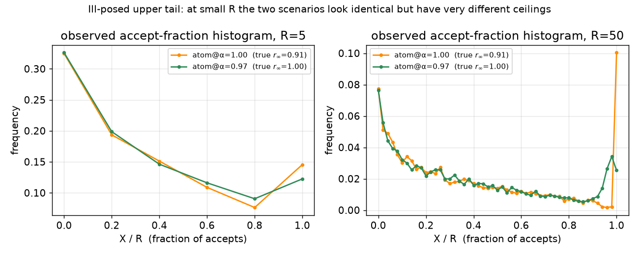
The inversion is a textbook ill-posed inverse problem, and honesty about resolution is part of the protocol: (P1) the ceiling is an upper-tail functional, and \(R\) verdicts cannot distinguish \(\alpha=1\) from \(\alpha=1-\epsilon\) below boundary resolution \(\epsilon\sim1/R\): two worlds with ceilings \(0.91\) and \(1.00\) produce nearly identical data at small \(R\) (Fig. 2), so ceiling estimates carry an \(R\)-dependent identifiability floor and require regularization — the exact structure (resolution kernels, damped inversion) long formalized for gross Earth data [15]; (P2) \(R\) verdicts identify only the first \(R\) moments: cheap protocols pin \(\rho_v\) but not the deep-\(k\) behavior; (P3) with a labeling budget \(B=NR\) there is an accuracy trade between instances and depth; low-order functionals favor large \(N\), tail functionals demand large \(R\).
5.0.0.2 Falsification loop.
The theory earns its keep by out-of-sample prediction: fit \(G\) at low order (small \(R\)), extrapolate the entire curve \(r_k\) to held-out gate depths, and compare. Exponential (\(\rho_v=0\)) and polynomial (\(\rho_v>0\)) predictions separate fast (Table 1), so modest data decide. A practical decision rule falls out: measure \(\widehat{\rho_v}\) with \(R=2\); if small, gates are cheap reliability (independence regime); if large, stop buying gates and spend on decorrelation — a different model family or modality, external oracles, tool-based verification. Even trivial perturbations that break the shared-blind-spot channel are known to help disproportionately [6].
5.0.0.3 Decorrelation vs.the exchangeability assumption.
One tension deserves to be stated head-on rather than left to the caveats. The lever the theory recommends — decorrelate the verifier from the generator by changing model family, modality, or evidence source — deliberately makes the gates heterogeneous, whereas Assumption 1 treats them as exchangeable under a single scalar \(\alpha\). The two are reconciled by reading “\(k\) gates” at the right granularity. (A) When the \(k\) gates are repeated draws of one verifier, or members of one blind-spot-sharing family, the scalar model is exact and the message is the pessimistic one: the extra gates inherit the same tail, so reliability saturates at the ceiling. (B) When the gates come from genuinely different families they are no longer exchangeable; the faithful object is a vector latent \(\boldsymbol{\alpha}=(\alpha_1,\dots,\alpha_k)\) (or a hierarchical \(G\)), and the present scalar theory is its first-order projection. That projection already points the right way: within the scalar model, splicing in a less-correlated gate is exactly what thins the effective upper tail of \(G\) — raising the exponent \(b\), shrinking the blind-spot mass \(1-\pi\), and lifting the ceiling \(-\ln(1-\pi)\). Decorrelation is thus not outside the theory’s logic but the operation that moves \(G\) in the one direction the scalar theory says matters; the faithful heterogeneous treatment — e.g.a rank-one shared-plus-family latent \(\alpha_i=\sigma(u+v_i)\), under which partial decorrelation registers as a measurable rise in \(b\) — is the natural sequel (§8).
6 Synthetic-recovery validation↩︎
Before touching real logs, we validate that the pipeline recovers known ground truth — the synthetic-recovery discipline standard in geophysical inversion. All experiments: \(N=4000\) instances, fixed seeds; code to reproduce all tables and figures is available at https://github.com/jianganghan/harness-verifier-cascades.
Data generated with \(\rho_v\in\{0.05,\dots,0.50\}\), \(\bar\alpha=0.3\), \(R=10\): the moment estimator recovers \(0.050/0.291/0.502\) at true \(0.05/0.30/0.50\); M2 agrees.
True \(\rho_v=0.30\): \(R=2\) yields \(\widehat{\rho_v}=0.274\); \(R\ge3\) is essentially exact — Proposition 10 in action.
Two worlds with \(10\%\) atom mass at \(\alpha=1.00\) vs.at \(\alpha=0.97\) (true ceilings \(r_\infty=0.91\) vs.\(1.00\)): at \(R=5\) their accept-count histograms are nearly indistinguishable (Fig. 2, left); at \(R=50\) the atom emerges and NPMLE assigns it mass \(0.100\) vs.\(0.000\) (right). \(\rho_v\) is cheap; the ceiling is expensive — exactly (P1)/(P2).
Fit beta-binomial on accept counts of order \(R=8\) only (\(\widehat{\rho_v}=0.30\)), extrapolate \(r_k\) to \(k\le25\): at \(k=5\) the correlated theory predicts \(0.954\) against truth \(0.953\), while the independence extrapolation from the same first-gate data gives \(0.998\) (Fig. 1).
The immediate next step is the same estimators on real accept/reject logs: tasks with programmatic ground truth (unit-tested code, exact-match extraction, numerically checkable math), the generator’s own wrong answers as the instance population, \(R\) verifier samples per instance — the protocol and code require only the data source to change.
7 Related work↩︎
7.0.0.1 Reliability algebra for harnesses.
The direct target is the Odds Law / Maestro Order pair [1], [5]: four primitives with composition laws, the \(\Lambda^\star=1\) threshold dichotomy, a water-filling controller, and — on the voting side — a latent-factor correlation theory with an effective-sample floor (Thm. 7.2 there). We modify exactly one assumption (conditional independence of verification gates) and answer the open problem stated there; our Corollary 1 recovers their Lemma 4.3/Thm. 5.1 as the \(\rho_v\to0\) boundary. The von Neumann lineage [4] is shared.
7.0.0.2 Correlated voting and ensembling.
Exchangeable-vote Condorcet theory dates to [9]; recent LLM-side treatments include non-monotone vote-scaling from difficulty heterogeneity [16], general de Finetti characterizations of when voting helps or hurts [3], and two-call moment identification of vote correlation [2] — the voting-side analogue of our Proposition 10. At the system level, hierarchical majority trees with a shared-error correlation exhibit a Kesten–Stigum-style amplification–collapse phase transition [17], and for answer-selection policies over a model pool (routing, voting, model cascades), [18] prove an accuracy ceiling of \(1-\beta\) — the pool’s simultaneous-failure rate — together with a negative identification result: pairwise error correlation cannot determine \(\beta\). Both concern correlated generators; our ceiling concerns correlated checking — the blind-spot atom of a generator–verifier family under conjunctive gating. The non-identifiability of [18] does not apply to Proposition 10, whose observable is repeated verdicts on the same instance rather than cross-model pairwise statistics; it is, however, consonant with our diagnosis that the tail quantity setting the ceiling is exactly the ill-posed direction of the inversion (§5). Verification is not voting: conjunctive gating induces the survivorship tilt of Remark 3, which has no one-shot-voting analogue, and yields phenomena absent there (per-gate evidence decay, the two-sided trichotomy, an internal \(k^\dagger\) at zero cost).
7.0.0.3 Self-verification blind spots.
That models systematically miss their own errors is documented empirically [6] and argued information-theoretically via a shared latent failure cause capping what self-evaluation can add [19]. We contribute the gating-algebra form of this idea: explicit finite-\(k\) posteriors, the concavity/polynomial/ceiling structure, closed forms in a one-parameter family — and a measurement protocol, which the information-theoretic treatment explicitly lacks.
7.0.0.4 Verifier/judge scaling and the exponential–polynomial dichotomy.
[20] obtain a finite optimal amount of judge-guided sampling when the reward model is misspecified; our regime (iii) is a distinct mechanism (correlation, not bias) for the same phenomenology, and the two are separable in data because \(\rho_v\) is directly measurable. That test-time reliability can decay polynomially rather than exponentially is by now a recurring finding: a knockout tournament’s failure probability decays exponentially or as a power law depending on how one scales [21], best-of-\(k\) under a misspecified reward yields polynomially diminishing returns [20], and attack-success curves show an explicit polynomial–exponential crossover set by the underlying generative mechanism [22]. We therefore do not claim the dichotomy itself as new; our contribution is to fix it to a specific mechanism — conjunctive survivorship against a blind-spot tail — for which the failure exponent is the closed form \(k^{-b}\) in \(G\)’s upper-tail index \(b\), controlled by the single measurable parameter \(\rho_v\). Empirical verification studies independently report that error-detectability falls with generator strength and that verifier scaling alone cannot overcome these correlation-driven limits [10].
8 Limitations and outlook↩︎
The theory is deliberately minimal. (1) Assumption 1 compresses all inter-gate structure into a scalar exchangeable latent — a mean-field idealization; gate-specific systematic differences (heterogeneous verifier families) call for a vector latent. (2) All-accept semantics: under generate–verify–retry, false rejections cost throughput rather than precision, which restores the one-sided picture for precision while making §4 the right model when regeneration is impossible or gates are terminal. (3) Beta is a convenience for closed forms; the asymptotics need only regularly-varying tails, and M3 removes the parametric assumption in estimation. (4) The validation here is synthetic recovery; the measurement on real generator–verifier pairs — the quantitative bridge both [1] and we regard as the natural sequel — is in progress, and the protocol of §5 is designed so that only the data source changes.
9 Deferred proofs↩︎
9.1 Theorem 4 (polynomial decay)↩︎
Proof. Substitute \(\alpha=1-s\): \(m_k=\int_0^1(1-s)^k g(1-s)\,ds\). The integrand is dominated by \(s=O(1/k)\); with \(g(1-s)\sim c\,s^{b-1}\) and \((1-s)^k=e^{k\ln(1-s)}\sim e^{-ks}\) on that scale, Watson’s lemma gives \(m_k\sim c\int_0^\infty e^{-ks}s^{b-1}ds=c\,\Gamma(b)\,k^{-b}\). For \(G=\mathrm{Beta}(a,b)\), \(m_k=\frac{B(a+k,b)}{B(a,b)}=\frac{\Gamma(a+b)}{\Gamma(a)}\cdot\frac{\Gamma(a+k)}{\Gamma(a+b+k)}\sim\frac{\Gamma(a+b)}{\Gamma(a)}k^{-b}\) by Stirling. Finally \(1-r_k=\frac{(1-p_0)m_k}{p_0+(1-p_0)m_k}\sim\frac{1-p_0}{p_0}m_k\). ◻
9.2 Corollary 2 (cost-optimal gates)↩︎
Proof. With \(1-r_k\approx\kappa k^{-b}\), marginal value \(U\frac{d r_k}{dk}\approx U\kappa b\,k^{-(b+1)}\); setting it equal to \(c\) gives \(k^{*}=(U\kappa b/c)^{1/(b+1)}\). Under independence \(1-r_k\approx\frac{1-p_0}{p_0}\bar\alpha^k\), and equating \(U\) times its derivative to \(c\) gives \(k^{*}=\Theta(\ln(U/c)/\ln(1/\bar\alpha))\). ◻
9.3 Theorem 7 (trichotomy)↩︎
Proof. Apply Appendix 9.1 to both moment sequences: \(m_k^{(\alpha)}\sim c_\alpha\Gamma(b_\alpha)k^{-b_\alpha}\), \(m_k^{(\beta)}\sim c_\beta\Gamma(b_\beta)k^{-b_\beta}\). Then 2 gives \(\ell_k=\ell_0+\ln\frac{c_\beta\Gamma(b_\beta)}{c_\alpha\Gamma(b_\alpha)}+(b_\alpha-b_\beta)\ln k+o(1)\). The three regimes read off the sign of \(b_\alpha-b_\beta\); in regime (i), \(1-r_k\sim\frac{1-p_0}{p_0}\frac{m_k^{(\alpha)}}{m_k^{(\beta)}}\asymp k^{-(b_\alpha-b_\beta)}\). ◻
9.4 Proposition 8 (crossover)↩︎
Proof. For Beta, the \(x^j\)-tilted distribution of \(\mathrm{Beta}(a,b)\) is \(\mathrm{Beta}(a+j,b)\) with mean \(\frac{a+j}{a+b+j}\), and \(\delta_{j+1}=\ln\frac{m^{(\beta)}_{j+1}/m^{(\beta)}_j}{m^{(\alpha)}_{j+1}/m^{(\alpha)}_j}\) is the stated ratio of tilted means. Setting \(\frac{a_\beta+j}{a_\beta+b_\beta+j}=\frac{a_\alpha+j}{a_\alpha+b_\alpha+j}\) and cross-multiplying, the \(j^2\) terms cancel, leaving the linear equation \(j(b_\alpha-b_\beta)=a_\alpha b_\beta-a_\beta b_\alpha\), whence \(k^\dagger\); linearity implies at most one sign change. If \(b_\alpha<b_\beta\) and \(\delta_1>0\), increments are positive for \(j<k^\dagger\) and negative after, so \(\ell_k\) (hence \(r_k\)) is unimodal with integer maximizer \(\lceil k^\dagger\rceil\). ◻
References↩︎
Independent researcher.
jiangangh@gmail.com.↩︎