Experience Memory Graph: One-Shot Error Correction for Agents
July 15, 2026
Abstract
Large Language Model (LLM) agents have shown remarkable capabilities in autonomous decision-making by generating sequential trajectories of states, actions, and observations. However, in complex, long-horizon tasks, these agents frequently suffer from compounding errors and struggle to recover from failures. Existing self-correction mechanisms rely on prompt-based reflection, which is inherently brittle, incurs heavy time and API costs due to iterative trial-and-error loops, and produces task-specific memory that may be hard to generalize to new scenarios. To address this, we propose Experience Memory Graph (EMG), a framework that reformulates agent failure recovery as a graph matching problem. At training time, we convert both failed exploration trajectories and successful expert trajectories into directed action decision graphs. By matching these graphs, we extract common subgraphs (successful workflows) and graph edit paths that explicitly indicate how to correct failures (e.g., which actions to add, delete, or relabel under a given observation), and store them in a memory graph with intra-task nodes and cross-task edges. At test time, EMG retrieves relevant insights and guides the agent in a single, loop-free execution. Experiments on ALFWorld and ScienceWorld show that EMG consistently outperforms state-of-the-art reflection baselines in success rate and average reward, while requiring no test-time trial-and-error.
<ccs2012> <concept> <concept_id>10010147.10010178</concept_id> <concept_desc>Computing methodologies Artificial intelligence</concept_desc> <concept_significance>500</concept_significance> </concept>
1 Introduction↩︎
Large Language Models (LLMs) have evolved from passive text assistants into autonomous agents with planning, memory, and tool-use capabilities, enabling closed-loop interaction with environments [1], [2]. This architecture has demonstrated strong zero‑shot and few‑shot performance across complex domains such as web navigation, multi‑step mathematical reasoning, and automated software engineering [3]–[5]. As agents act iteratively, they generate long‑horizon trajectories—sequential structures of states, actions, and observations. Rather than being mere logs, these trajectories contain rich, reusable experience. By systematically extracting successful workflows and failure patterns from past trajectories, agents can build experience memory that helps avoid repeated mistakes and improve task success rates on subsequent attempts [6], [7].
To construct experience memory from interaction trajectories, early approaches relied exclusively on extracting workflows from successful executions [8], [9]. Subsequent methods have increasingly leveraged failed trajectories to enhance learning. While some studies focus on isolating decisive erroneous actions or performing failure credit assignment [10]–[12], others extend this paradigm by actively rectifying failed trajectories to achieve task success [13]–[25]. Typically, these approaches prompt LLMs to reflect on the root causes of failure—specifically, identifying the erroneous action and hypothesizing a corrective counterpart. The model then replays the task grounded in this refined memory, thereby constituting an iterative reflect-and-replay mechanism, as illustrated in Fig. 1(a). While previous methods successfully construct memory by rectifying failed trajectories and achieve impressive performance, they suffer from three primary limitations.
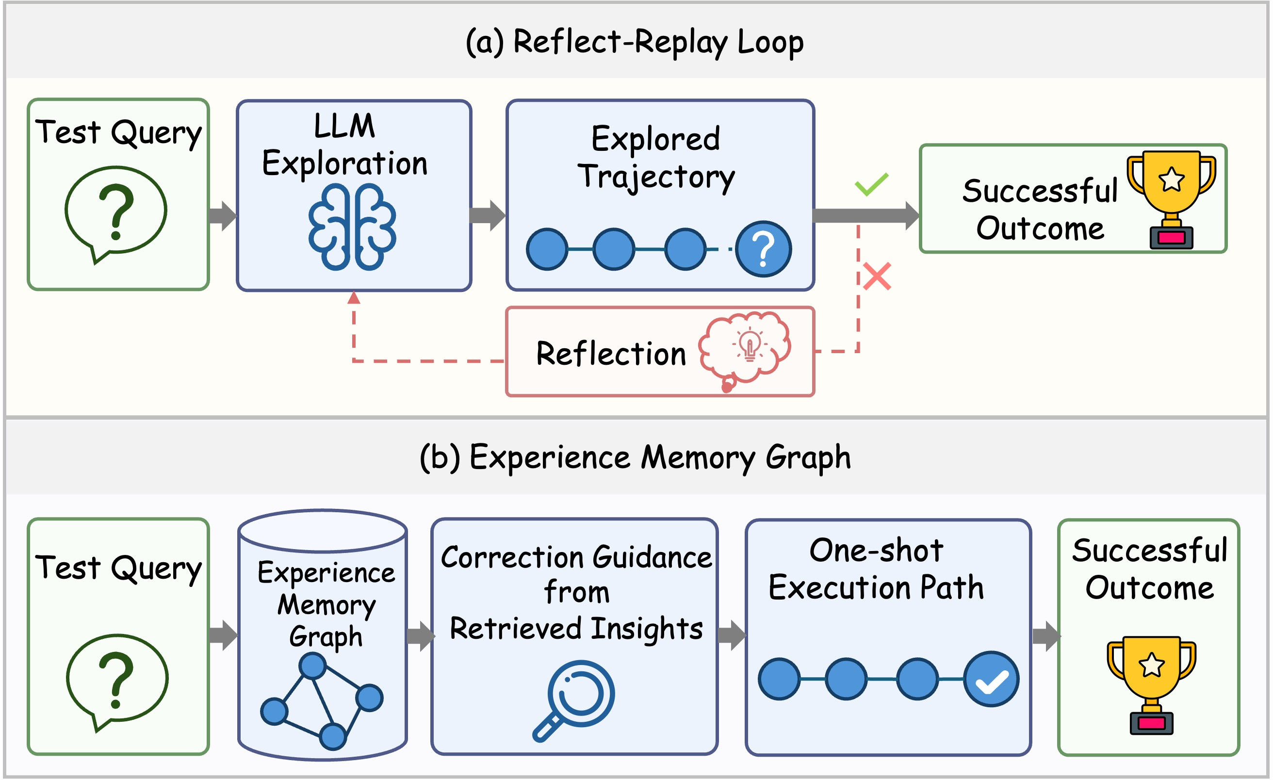
Limitation 1: Dependence on LLM Capabilities. This prompt-based reflection paradigm can be sensitive to prompt design, and its effectiveness is often constrained by the model’s inherent capabilities.For instance, smaller LLMs usually struggle to break out of repetitive error cycles, which can hinder their ability to perform effective self-reflection and correction. Moreover, in long-horizon trajectories, accurately identifying the root cause of a failure — which may be deeply buried in a long sequence of states and actions — can be challenging for such models.
Limitation 2: Inference Cost. After each failure, the model needs to reflect, adjust, and re-execute the trajectory. This iterative looping process multiplies both latency and API costs. In commercial or real-time scenarios, such back-and-forth loops may become less efficient, potentially limiting their practicality for time-sensitive applications.
Limitation 3: Limited Cross-Task Generalization. Most existing approaches perform reflection and re-execution directly on the test set for individual failed tasks, rather than extracting reusable memory from training failures. Consequently, the synthesized memory is task-specific, resulting in limited transferability to unseen scenarios.
To address these issues, we propose Experience Memory Graph (EMG), a novel framework that shifts the paradigm from online LLM reflection to offline, deterministic graph computation. EMG structures memory as a comprehensive network where nodes store localized task knowledge (successful workflows or corrective paths for individual tasks) and edges capture generalized action patterns across similar tasks. To construct each node in the experience memory graph, we convert both the failed exploration trajectory and the successful expert trajectory of the same training task into action decision graphs. By performing graph matching between them, we extract the common subgraph (representing correctly executed workflows) and compute the shortest graph edit path. This path serves as a deterministic, one-shot error correction plan—dictating exactly which actions to retain, delete, or replace under specific observations. By relying on algorithmic exactness rather than prompt-based guessing, this mechanism robustly localizes root errors and fully resolves the over-reliance on LLM capabilities (Limitation 1). To construct each edge in the experience memory graph, we further connect semantically similar task queries (via top-\(k\) nearest neighbors) and perform graph matching between their respective expert trajectories. This process extracts cross-task insights stored on the edges, capturing reusable, high-level action patterns that transfer across different scenarios. Crucially, the entire memory construction is performed offline on the training set. Once built, this memory graph can be applied to any test set, directly addressing the limited generalizability of task-specific memory (Limitation 3). During test-time inference, the agent simply retrieves the pre-computed correction paths and cross-task insights without any iterative trial-and-error, thereby circumventing the prohibitive inference overhead and API costs (Limitation 2). This makes EMG a highly efficient and accurate solution for real-time applications. In summary, our contributions are three-fold:
We propose Experience Memory Graph (EMG), a novel framework that structures experience for LLM agents as a relational graph. By organizing memory into nodes for localized task knowledge and edges for generalized action patterns, EMG enables robust cross-task generalization that surpasses traditional task-specific memory banks.
We introduce a deterministic memory acquisition mechanism based on graph matching to populate EMG. By extracting the common subgraph to preserve successful workflows and computing the shortest graph edit path for one-shot error correction, our approach replaces brittle, iterative LLM reflection loops with algorithmic exactness, significantly reducing API costs and latency.
Extensive experiments on challenging benchmarks demonstrate that EMG significantly outperforms state-of-the-art self-reflection baselines. Notably, EMG exhibits superior performance and computational efficiency in long-horizon tasks requiring complex reasoning.
2 Related Work↩︎
2.1 Experience Memory↩︎
Experience memory aims at extracting the reusable workflow and insight from history trajectories. Early studies on experience memory construction mainly extract reusable workflows from successful trajectories [8], [9], assuming that successful executions directly encode high-quality procedural knowledge. However, such approaches ignore informative signals from failed trajectories.
To leverage failures, some works focus on failure diagnosis. AgenTracer [10] leverages counterfactual replay and fault injection to perturb trajectories and trace back the root cause of failures, enabling fine-grained attribution to specific actions or modules. Trajectory graph copilot [11] models trajectories as a graph structure and applies graph neural networks to capture temporal dependencies and detect error-prone action patterns, allowing pre-action diagnosis. AgentDebug [12] further conducts a large-scale empirical study of LLM agent failures, categorizing error types and revealing common failure modes.
Another line of work focuses on correcting failed trajectories via reflection [26], [27]. R2D2 [14] performs step-level reflection to locate the first erroneous action, truncates the trajectory from that point, and stores corrected sub-trajectories along with reflections for future reuse. ReasoningBank [13] goes beyond trajectory replay by abstracting experiences into reusable high-level reasoning strategies, improving generalization across tasks. Building on this paradigm, principles [15] learns synthetic strategy memory for proactive decision-making, Memp [16] introduces procedural memory that captures action-level execution knowledge, and some works [17], [18], [28] organize experiences into structured or graph-based skill representations to enhance compositionality. Moreover, CDMem [19] additionally improves context-aware memory retrieval, and [20] explicitly trains agents to learn sequential decision policies from failed attempts.
These methods typically follow a reflect–replay paradigm, where the agent first analyzes failure causes (e.g., identifying erroneous actions and suggesting corrections), then re-executes the task using refined memory. Despite their effectiveness, they often rely heavily on the quality of reflection and may suffer from inefficient iterative correction or error propagation.
2.2 Graph for Agent Memory↩︎
Recent studies have explored graph memory mechanisms to enhance long-term reasoning and experience reuse in LLM agents [29]. AriGraph [30] constructs a unified graph that integrates semantic and episodic memories for planning and reasoning in interactive environments. A-Mem [1] further enables autonomous memory evolution by dynamically linking and restructuring memories into an interconnected knowledge network. G-Memory [31] extends graph-based memory to multi-agent settings through hierarchical interaction and insight graphs, facilitating cross-trial knowledge transfer. Recent efforts such as SGMem [32], GAM [33], and H-Mem [34] further investigate sentence graphs, hierarchical graph memories, and hybrid graph-based memory evolution mechanisms to enhance long-horizon retrieval and adaptive reasoning capabilities.
Despite encouraging progress, existing methods mainly focus on memory storage and retrieval, while the extraction of reusable high-level insights and the modeling of transferable experience relationships remain underexplored. Our EMG fills this gap by using graph matching to derive common subgraphs and edit paths, transforming raw trajectories into transferable correction workflows.
3 Preliminary↩︎
We consider LLM-based agents that interact with environments to solve long-horizon tasks. Following prior work, we formulate such agentic tasks as a partially observable Markov decision process (POMDP) without explicitly modeling the latent state. The process is defined by the tuple \((\mathcal{Q}, \mathcal{A}, \mathcal{O}, T, R)\), where \(\mathcal{Q}\) is the query (instruction) space, \(\mathcal{A}\) the action space, \(\mathcal{O}\) the observation space, \(T: \mathcal{A} \times \mathcal{O} \rightarrow \mathcal{A}\) a transition function that determines the next action given the current action and observation, and \(R: \mathcal{A} \times \mathcal{O} \rightarrow [0,1]\) the reward function. Since our focus is on the task planning capability of LLM agents, \(\mathcal{Q}\), \(\mathcal{A}\), and \(\mathcal{O}\) are subsets of the natural language space.
Given a task query \(q \in \mathcal{Q}\), the LLM agent \(\pi_\theta\) interacts with the environment as follows. At each time step \(t\), the agent samples an action \(a_t \sim \pi_\theta(\cdot \mid q, \tau_{t-1})\) based on the query and the history of previous interactions. It then receives environmental feedback as an observation \(o_t \in \mathcal{O}\). The historical interaction trajectory up to step \(t-1\) is denoted by \(\tau_{t-1} = (o_0, a_1, o_1, a_2, o_2, \ldots, a_{t-1}, o_{t-1})\), where \(o_0\) is the initial observation of the environment before any action is taken. The interaction loop continues until the agent either completes the task or reaches the maximum allowed number of steps. The complete trajectory is written as \(\tau = (q,\, o_0,\, a_1,\, o_1,\, a_2,\, o_2,\, \ldots,\, a_m,\, o_m)\), where \(o_0\) is the initial observation of the environment, and \(m\) denotes the trajectory length. Finally, a reward \(r (q, \tau) \in [0,1]\) is assigned to indicate whether the task is successfully completed or has failed.
4 Method↩︎
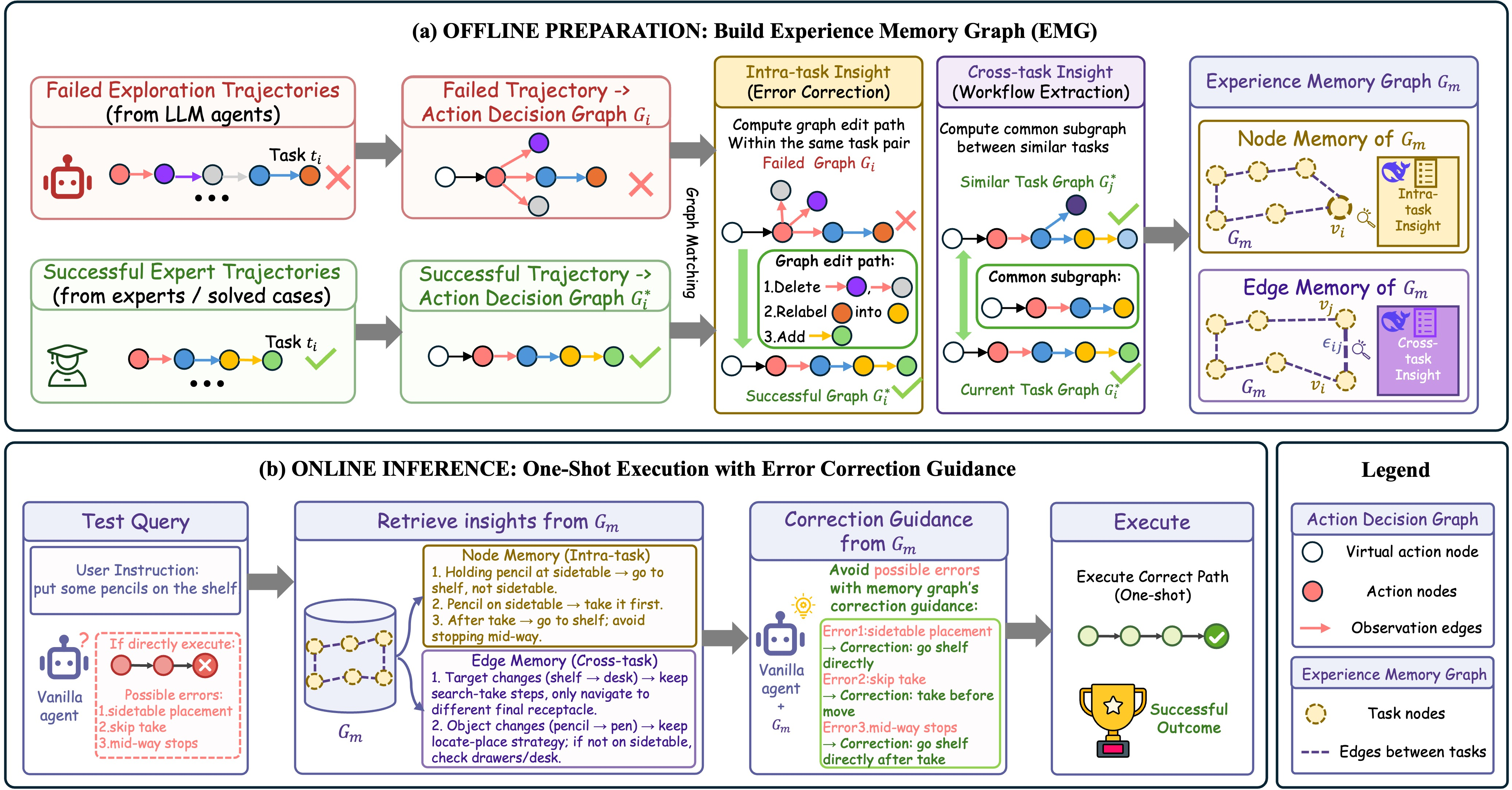
In this section, we present Experience Memory Graph (EMG), a framework that constructs structured experience memory from training tasks and applies it to new tasks, which is shown in fig. 2. The overall pipeline consists of three stages: (1) preparing training trajectories and converting them into action decision graphs; (2) constructing a memory graph where nodes store intra-task insights and edges store cross-task insights; and (3) retrieving relevant memory at test time to guide the agent without additional loops. We detail each stage below.
4.1 Preparation↩︎
Before constructing the experience memory graph, we first collect trajectories on the training tasks and convert them into action decision graphs.
4.1.1 Collecting Exploration Trajectories↩︎
For each training task query \(q\) in the training set \(\mathcal{Q}_{\text{train}}\), we let an LLM agent interact with the environment to produce a single exploration trajectory \(e_m\) (which may either succeed or fail). For the same task \(t_i\), we assume access to a successful expert trajectory \(\tau_i^*\), provided by datasets such as ETO [35]. Thus, for each training task, we obtain a pair \((\tau_i, \tau_i^*)\). Failed exploration trajectories are particularly valuable, as they contain mistakes that can be corrected; successful ones can be used as positive examples directly. We collect such pairs over all training tasks.
4.1.2 Transforming Trajectories into Action Decision Graphs↩︎
To explicitly model the decision process — which action should be taken under a given observation — we convert each raw trajectory into a directed action decision graph. A successful trajectory and a failed one often differ precisely in this decision mapping. By constructing a graph where nodes are actions and edges carry the preceding observation, we make explicit the rule: for a given state, which action is chosen. This decision‑centric representation enables the graph edit path to learn meaningful correction insights — e.g., under a specific observation, which wrong action should be replaced by which correct action. Compared to raw sequential sequences, where the same action may appear in different contexts without a clear link to the triggering observation, our graph formulation yields far more actionable and transferable correction knowledge.
Graph representation. We denote the action decision graph as \(G = (V, E, q, r)\), where \(q\) is the task query and \(r\) is the final reward. Nodes represent actions, edges represent the observations preceding those actions. To obtain compact yet discriminative representations for labeling, we normalize each action into a tuple \(k = (\text{type}, \text{object}, \text{receptacle})\) (e.g., \((\text{take}, \text{apple}, \text{table})\)), capturing the action type and the objects it operates on; the raw action text \(a_v^{\text{raw}}\) (e.g., "take apple from table") is also kept. Each node is represented as \(v_i = (k_i, a_i^{\text{raw}}, \ell_n(v))\) with node label \(\ell_n(v_i)\in\mathbb{N}\). A virtual INIT node \(v_{\text{init}}\) (\(\ell_n(v_{\text{init}})=0\)) provides an incoming edge for the first action, carrying the initial observation \(o_0\).
Each directed edge is denoted as \(e_i = ((v_i, v_{i+1}), s_i, \ell_e(e_i)) \in E\). \((v_i, v_{i+1})\) represents the connection from action node \(v_i\) to \(v_{i+1}\). So \(e_i\) is both the observations resulting from the action \(v_i\) and the preceding observation of the next action \(v_{i+1}\). \(e_i\) also carries a normalized observation text \(s_i\) derived from the raw observation \(o_i\) (e.g., “kitchen: apple, potato”) and its edge label \(\ell_e(e_i) \in \mathbb{N}\).
Construction design. Two design choices ensure the action decision graph captures decision-level information. 1. node reuse: if the same normalized action tuple appears multiple times in the trajectory, we do not create a new node; instead, we reuse the existing node. This gives the node multiple incoming edges, each associated with a different preceding observation, thus capturing the decision pattern that the same action may be taken under various observed states. 2. parallelizing consecutive invalid actions: when an action leads to an uninformative observation (e.g., “nothing happens”), the environment state does not change. We keep the current valid state unchanged and connect all such invalid actions from the same previous valid node, treating them as parallel attempts from the same decision point rather than a spurious chain.
To implement these ideas, we scan the trajectory once, maintaining the current valid state \(s\) (initialized as normalized \(o_0\)) and the node \(last\) (initially \(v_{\text{init}}\)) that produced it. A dictionary \(\Phi\) maps each normalized action tuple to its node, enabling node reuse. The detailed Algorithm 7 and a concrete example is available in Appendix A. After building the structure, we assign labels: each distinct action tuple \(k\) receives a unique positive integer as node label \(\ell_n(v)\) (0 for \(v_{\text{init}}\)), and each distinct normalized observation text \(s\) receives a unique positive integer as edge label \(\ell_e(e)\). Thus, identical contents yield identical labels, allowing graph matching to compare semantics by simple label equality.
The resulting action decision graph abstracts raw action and observation texts into discrete labels (node labels for action tuples, edge labels for observation texts), enabling efficient structure comparison via label equality in the subsequent graph matching stage. At the same time, each node and edge preserves the original raw texts, which are later used to convert extracted common subgraphs and graph edit paths into natural‑language insights.
4.2 Construction of Experience Memory Graph↩︎
To move beyond test‑time self‑reflection, we build an offline experience memory graph that stores structured, reusable experience. This memory graph provides two key benefits: (1) it captures precise error corrections and successful workflows for individual tasks, and (2) it generalizes across similar tasks by extracting shared decision patterns. To construct such a memory graph, we leverage graph matching on the action decision graphs obtained from Section 4.1. By matching failed exploration graphs with their corresponding expert graphs, we extract intra‑task common subgraphs and graph edit paths; by matching expert graphs of semantically similar tasks, we obtain cross‑task insights. These structured pieces of knowledge are organized into the experience memory graph \(\mathcal{G}_m=(\mathcal{V},\mathcal{E})\), where each node \(\nu \in\mathcal{V}\) stores intra‑task insights and each edge \(\epsilon \in\mathcal{E}\) stores cross‑task reusable insights. We first define the experience memory graph formally.
Let \(\mathcal{V} = \{\nu_1,\dots,\nu_N\}\) where each node \(\nu_i\) is a tuple: \[\nu_i = \bigl(q_i,\; {embed}_i,\; I_i^{\text{intra}},\; G_i,\; G_i^*,\;r_i\; \bigr), \label{eq:memory95node}\tag{1}\] where \(q_i\) is the task query, \({embed}_i\) the query embedding, \(I_i^{\text{intra}}\) is the intra‑task insight, and \(G_i, G_i^*\) are the action decision graphs of the exploration trajectory and the expert trajectory, respectively (built via Algorithm 7). \(r_i\in\{0,1\}\) is the reward (success/failure) of exploration trajectory \(G_i\), and the reward of expert trajectory is always 1 and we omit it here.
Each edge \(\epsilon_{ij}\in\mathcal{E}\) connects \(\nu_i\) and \(\nu_j\) and is defined as: \[\epsilon_{ij} = \bigl(s_{ij},\; I_{ij}^{\text{cross}}\bigr), \label{eq:memory95edge}\tag{2}\] where \(s_{ij} = \cos({embed}_i,{embed}_j)\) is the cosine similarity between query embeddings, and \(I_{ij}^{\text{cross}}\) is the cross‑task insight text.
4.2.1 Constructing Node Insights↩︎
Recall that \(G_i\) and \(G_i^*\) are the action decision graphs built from the raw exploration and expert trajectories using the method in Section 4.1. This graph representation allows us to compare them structurally via graph matching. Given a pair of exploration graph \(G_i\) and expert graph \(G_i^*\), we can extract two kinds of structured knowledge: the common subgraph \(G_i^c\) (the correct actions in the failed trajectory that should be maintained, revealing the successful workflow) and the graph edit path \(G_i^e\) (a sequence of edit operations that transforms failed exploration \(G_i\) into successful expert \(G_i^*\)), from \(G_i^e\) we directly obtain: (a) which actions to add or avoid under specific observations (from node deletions/insertions), and (b) which action to replace with another under a given observation (from relabeled actions). To compute \(G_i^c\) and \(G_i^e\), we first find a node matching between the two graphs via graph matching, then we compare the two graphs: the parts that are identical in both structure and labels form the common subgraph; the differences (mismatched nodes and edges) directly yield the graph edit path. Thus, instead of test‑time trial‑and‑error, we directly obtain correction instructions and successful workflows.
Concretely, we first obtain the node matching between \(G_i\) and \(G_i^*\) via graph matching. Since supervised matching heavily relies on ground‑truth node correspondences, we adopt an unsupervised approach based on optimal transport (OT). Most OT‑based methods adopt the Fused Gromov‑Wasserstein (FGW) distance [36], [37], which jointly considers node labels and edge structures. For two graphs \(G\) and \(G'\) with soft assignment \(\pi \in \mathbb{R}^{|V| \times |V'|}\), our FGW objective is: \[\mathrm{FGW} = \min_{\pi} \sum_{i,j} C_{ij}\pi_{ij} + \sum_{i,j,k,l} |A_{ij}^g - A_{kl}^{g'}|^2 \pi_{ik}\pi_{jl}, \label{eq:fgw}\tag{3}\] where \(\pi_{ij}\) indicates the matching strength between node \(i\) in \(G\) and node \(j\) in \(G'\), \(C_{ij}\) is the cost of relabeling node \(i\) to \(j\), and \(A^g, A^{g'}\) are adjacency matrices. Unlike the standard FGW formulation which includes a factor \(\frac{1}{2}\) for undirected graphs where each edge is counted twice) [36], [37], our directed graphs require no such factor, and we drop it. We adopt the FGWAlign solver [36] to optimize this objective, which supports edge-labeled graphs. The time complexity of the solver is \(O(|\mathcal{V}|^3 \cdot |\mathcal{L}|)\), where \(|\mathcal{L}|\) is the number of edge label types. Since our trajectory graphs typically contain at most a few dozen nodes, the solver is highly efficient.
After obtaining the optimal soft plan \(\pi^*\), we discretize it into a hard node matching matrix \(P \in \{0,1\}^{|V| \times |V'|}\) via linear assignment: \[P = \arg\max_{P \in \mathbb{P}_n} \langle \pi^*, P \rangle, \label{eq:linear95assignment}\tag{4}\] where \(\mathbb{P}_n\) denotes the set of permutation (or partial permutation) matrices. Each entry \(P_{ij}=1\) indicates that node \(i\) in \(G\) is matched to node \(j\) in \(G'\).
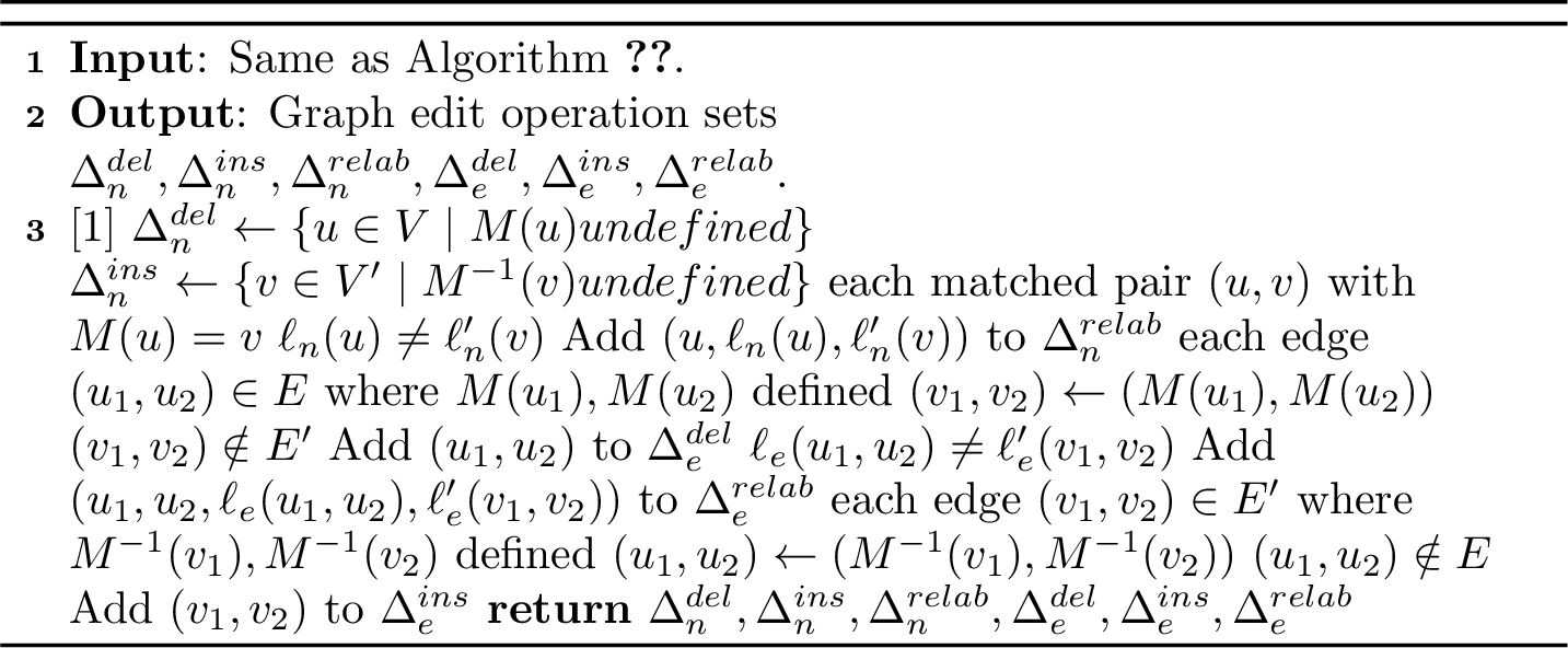
Given the node matching matrix \(P\), we define a node matching \(M: V \mapsto V'\) where \(M(u)=v\) if \(P_{uv}=1\) (and \(u\) is unmatched if no such \(v\) exists), then we derive the graph edit path and the common subgraph by comparing the two graphs. Classical methods for extracting edit paths and common subgraphs are designed for undirected graphs with only node labels; they cannot handle edge labels and do not respect edge directions. Directly applying them to our directed edge‑labeled action decision graphs would discard the semantic information carried by edge observations (the preconditions of actions). Therefore, we adapt these methods to our setting. Specifically, Algorithm 8 retains edges that exist in both graphs with identical labels under the matching (the correct workflow); Algorithm 9 collects unmatched or mismatched nodes and edges to form edit operations (deletions, insertions, relabelings), directly indicating the necessary corrections. The detailed algorithm is available in Appendix B.
Finally, we generate the intra‑task insight. If the exploration succeeded (\(r_i=1\)), we retain the common subgraph \(G_i^c\) (extracted via Algorithm 8) as the correct workflow. If it failed (\(r_i=0\)), we use the graph edit path \(G_i^e\) (via Algorithm 9) as the correction instructions. For environments with continuous reward (e.g., ScienceWorld), a partially successful trajectory (\(0<r_i<1\)) contains both correct and incorrect actions; we therefore feed both \(G_i^c\) (to preserve the correct actions) and \(G_i^e\) (to correct the errors) to the LLM. In all cases, the LLM takes the task query \(q_i\) as input, the original exploration graph \(G_i\), the expert graph \(G_i^*\), and the extracted structure(s) \(X_i\) (where \(X_i\) is \(G_i^c\) (\(r_i=1\)), or \(G_i^e\) (\(r_i=0\)), or both (\(0<r_i<1\))), and summarizes them into intra-task insight: \[I_i^{\text{intra}} = \mathrm{LLM}\bigl( \text{intra-prompt}(q_i, G_i, G_i^*, X_i) \bigr). \label{eq:intra95insight}\tag{5}\]
In summary, \(I_i^{\text{intra}}\) supplies either the correct workflow or explicit corrections, enabling test‑time guidance without trial‑and‑error.
4.2.2 Constructing Edge Insights↩︎
Using the action decision graph representation for all expert trajectories, we can compare the successful decision patterns of different tasks. We further aim to extract generalizable knowledge that transfers across similar tasks (e.g., different environments with analogous goals). For two task nodes \(\nu_i\) and \(\nu_j\) with similar queries in the memory graph, comparing their expert graphs \(G_i^*\) and \(G_j^*\) via graph matching reveals a common subgraph — actions that are correct under similar observations in different environments which should be learned and maintained. This provides cross‑task insights that are robust to environmental variations.
To realize this, after building all nodes we compute pairwise query embedding similarities \(s_{ij} = \cos({embed}_i, {embed}_j)\), where \({embed}_i\) is the embedding of node \(\nu_i\)’s query. An edge \(\epsilon_{ij}\) is added if \(s_{ij} \ge \tau\), and we only connect each node to its top-\(k\) most similar neighbors. For each edge \(\epsilon_{ij}\) connecting node task \(\nu_i\) and \(\nu_j\), we perform graph matching between the expert graphs \(G_i^*\) and \(G_j^*\) of \(\nu_i\) and \(\nu_j\), and use the same adapted FGW solver and Algorithm 8 to obtain the common subgraph \(G_{ij}^c\). We then prompt an LLM to summarize \(G_{ij}^c\) into the cross‑task insight: \[I_{ij}^{\text{cross}} = \mathrm{LLM}\bigl( \text{cross\_prompt}(q_i, q_j, G_i^*, G_j^*, G_{ij}^c) \bigr). \label{eq:cross95insight}\tag{6}\] This insight is stored on the edge \(\epsilon_{ij}\), which can guide the agent when facing new tasks similar to either endpoint.
4.3 Retrieval of Experience Memory Graph↩︎
During test time, given a new task query \(q_{\text{test}}\), we first embed it using the same embedding model to obtain \({embed}_{\text{test}}\). The similarity to each memory node \(\nu_i\) is computed as \(s_i = \cos({embed}_{\text{test}}, {embed}_i)\). We retrieve the top-\(K\) nodes with the highest \(s_i\). For each such node \(\nu_i\), we also retrieve the most relevant cross‑task insights: we look at all edges incident to \(\nu_i\), and for each neighbor \(\nu_j\) we compute its similarity to \(q_{\text{test}}\) as above. The edges with the top-\(T\) neighbor similarities are selected, and their stored cross‑task insights are collected. Formally, the retrieval result for \(q_{\text{test}}\) is: \[\mathcal{R}(q_{\text{test}}) = \bigcup_{\nu_i \in \text{TopK}} \left\{ \bigl( I_i^{\text{intra}},\; \{ I_{ij}^{\text{cross}} \mid \nu_j \in \text{TopT}(\nu_i) \} \bigr) \right\}, \label{eq:retrieval}\tag{7}\] where \(\text{TopT}(\nu_i)\) are the neighbors of \(\nu_i\) with the highest query similarities. The retrieved insights, derived from structured graph comparisons, provide concrete decision rules, making them directly usable for the agent. For instance, when faced with a task such as “put some pencil on shelf,” the retrieved node insight may specify that once the agent is holding the pencil at the sidetable, the correct next action is to go directly to the shelf rather than placing it elsewhere, and that the action of taking the pencil must precede any movement toward the target. The retrieved edge insights further provide cross‑task guidance, such as adapting the final navigation step when the target changes from shelf to desk, or expanding the search strategy when the object changes from pencil to pen. These insights are then passed to the agent’s prompt as guidance, eliminating any need for test‑time reflection or trial‑and‑error loops.
The complete Experience Memory Graph \(\mathcal{G}_m\) is built offline on the training set. Its construction cost is amortized over many test tasks, and the retrieval is fast (embedding similarity + neighbor lookup). This makes EMGboth efficient and scalable.
5 Experiments↩︎
5.1 Experimental Settings↩︎
| Dataset | #Train | #Test-Seen | #Test-Unseen | |
|---|---|---|---|---|
| ALFWorld | 3321 | 140 | 134 | |
| ScienceWorld | 1483 | 194 | 211 |
5.1.1 Datasets↩︎
We conduct experiments across two mainstream datasets: ALFWorld and ScienceWorld. The detailed statistics are summarized in Table 1. ALFWorld provides embodied household tasks to assess the agent’s capacity for spatial memory and sequential execution in everyday scenarios. ScienceWorld simulates interactive science experiments and features the longest trajectories, serving as a rigorous benchmark for evaluating long-term memory retention, multi-step planning, and complex scientific reasoning. To measure both in-distribution learning and out-of-distribution generalization capabilities, we evaluate agent performance on both seen and unseen test splits for ALFWorld and ScienceWorld with the same split of ETO [35]. The reward of ALFWorld is either 0 or 1, and the reward of ScienceWorld is from 0 to 1.
5.1.2 Baselines↩︎
In this paper, we benchmark our EMG against a spectrum of representative frameworks, containing both methods with reflect-replay loop and memory construction. We first consider ReAct [38], a widely adopted prompting strategy that interleaves reasoning traces with task-specific actions, serving as our fundamental memory-less baseline. Reflexion [39] enables the agent to leverage short-term episodic memory of past mistakes to iteratively refine its behavior within a single environment. Extending beyond transient self-reflection, we evaluate ExpeL [40], which accumulates rules from historical trajectories, acting as an experiential learning baseline. Furthermore, we compare against recent CDMem [19], which constructs both short-term memory and long-term memory based on reflection, and MemP [16], which explicitly constructs procedural memory to reuse complex execution routines. Our EMG adopts ReAct as the base model and retrieves insights in the constructed memory graph when testing. Each baseline is equipped with few-shot examples. For baselines with reflect-replay loop (Reflexion, Expel and CDMem), we run for 5 iterations.
5.1.3 Evaluation Metrics and Settings↩︎
We employ two commonly used metrics: Success Rate (SR) and Average Reward (AR). While SR acts as the primary indicator of ultimate task completion, AR provides a granular assessment of partial progress and intermediate sub-goal achievement, reflecting the agent’s step-by-step reasoning and memory utilization throughout long-horizon interactions. We apply DeepSeek V3.2 (chat mode) to collect exploration trajectories, and construct the experience memory graph with DeepSeek V3.2 (chat mode) for Scienceworld, and Deepseek V4-flash (chat mode) for ALFWorld. For testing tasks, we use both the open-source small model Qwen3:4B-instruct-2507-q8 and the large model DeepSeek-V4 flash (chat mode) to compare the performance of baselines.
| Method | ALFWorld | ScienceWorld | Avg. | |||||
|---|---|---|---|---|---|---|---|---|
| 3-4 (lr)5-8 | S-SR | U-SR | S-AR | S-SR | U-AR | U-SR | ||
| ReAct | 29.29 | 21.64 | 33.19 | 11.86 | 30.57 | 8.53 | 22.51 | |
| Reflexion | 34.29 | 39.55 | 39.25 | 30.06 | 8.06 | 27.69 | ||
| ExpeL | 39.55 | 13.40 | ||||||
| CDMem | 27.14 | 32.84 | 29.99 | 13.92 | 23.13 | 8.53 | 22.59 | |
| MemP | 37.86 | 26.83 | 9.28 | 25.20 | 8.53 | 25.04 | ||
| EMG | ||||||||
| ReAct | 86.43 | 88.06 | 17.53 | 13.74 | ||||
| Reflexion | 82.86 | 47.12 | 12.89 | 43.92 | 8.06 | 47.53 | ||
| ExpeL | 81.43 | 83.58 | 46.56 | 44.90 | 48.45 | |||
| CDMem | 31.91 | 15.46 | 35.38 | 8.53 | 46.22 | |||
| MemP | 85.71 | 85.82 | 44.73 | 10.31 | 44.78 | 11.37 | 47.12 | |
| EMG | ||||||||
5.2 Main Results↩︎
The main results are presented in Table 2. An analysis of these results reveals three key insights as follows.
Consistent Superiority over Iterative Paradigms. Across both datasets and all evaluation splits, EMG consistently outperforms all baseline methods in terms of SR and AR with both small and large models. Notably, our method demonstrates a clear advantage over frameworks based on reflect-replay loop such as Reflexion, ExpeL, and CDMem. Those baselines rely on reasoning about erroneous actions and re-executing attempts to self-correct. While our EMG directly uncovers the correct correction paths from the training set and constructs memory, thereby guiding test-time decisions more reliably and achieving higher success rates.
Overcoming the Reasoning Bottleneck of Compact LLMs. The performance gap between EMG and the baselines is more evident for the smaller Qwen3-4B than for the larger DeepSeek-V4-Flash, specially for ALFWorld. Iterative frameworks like expel require strong intrinsic reasoning to analyze past mistakes and derive alternative actions, the capacity that smaller LLMs often lack. By providing insights from error correction and workflow, EMG helps smaller models overcome this limitation, leading to substantially larger relative gains compared to large models.
Moreover, when adopting DeepSeek for testing, although iterative baselines are equipped with DeepSeek model for better reflection, they still underperform EMG, suggesting that the structured extraction of corrections and workflows provides additional benefits that scaling alone and iterative reflection do not fully capture.
Bridging the Scale Gap in Complex Tasks. The efficacy of EMG is highlighted in the highly demanding ScienceWorld environment, which necessitates intricate multi-step scientific reasoning. Remarkably, the 4B-parameter Qwen3 model equipped with EMG achieves performance comparable to—and in some metrics exceeding—the significantly larger DeepSeek model running standard baselines. This suggests that our EMG can effectively polish the capacity of small models when tackling complex, long-horizon decision-making problems.
| Method | ALFWorld | ScienceWorld | |||||
|---|---|---|---|---|---|---|---|
| 3-4 (lr)5-8 | S-SR | U-SR | S-AR | S-SR | U-AR | U-SR | |
| w/o NE | 29.29 | 21.64 | 33.19 | 11.86 | 30.57 | 8.53 | |
| w/o E | 48.57 | 52.99 | 34.84 | 12.37 | 35.77 | 9.48 | |
| 53.57 | 60.45 | 49.74 | 17.53 | 46.76 | 16.11 | ||
| w/o NE | 86.43 | 88.06 | 51.77 | 17.53 | 52.69 | 13.74 | |
| w/o E | 91.43 | 95.52 | 60.54 | 29.38 | 58.87 | 23.22 | |
| 96.43 | 97.76 | 62.37 | 28.87 | 61.94 | 24.17 | ||
5.3 Ablation Study↩︎
To isolate the contributions of each component, we evaluate two ablated variants: EMG w/o NE: removing both node’s intra-task insights and edge’s cross-task insights, and it is actually ReAct without memory; EMG w/o E: removing only the edge’s cross-task insights and retaining node’s intra-task insights. The results are detailed in Table 3, from which we draw three principal conclusions.
Crucial Role of Intra‑Task Node Memory. Comparing EMG w/o NE (no memory) with EMG w/o E (node only) shows that node memory alone brings substantial gains in most cases. For instance, DeepSeek’s Unseen SR in ScienceWorld jumps from 13.74% to 23.22%, and Qwen’s Unseen SR in ALFWorld from 21.64% to 52.99%. However, on ScienceWorld with the small Qwen model, the improvement is modest (Seen SR: 11.86% → 12.37%; Unseen SR: 8.53% → 9.48%), suggesting that extremely complex reasoning may still require additional cross‑task support. Overall, node memory serves as a solid foundation, effectively preventing repeated failures where the task is within the model’s basic reasoning capacity.
Differential Sensitivity to Cross‑Task Insights. Adding edges (comparing EMG w/o E to full EMG) yields asymmetric gains. The small Qwen3-4B benefits noticeably from cross‑task insights, e.g., ScienceWorld Unseen SR rises from 9.48% to 16.11%. In contrast, the large DeepSeek gains marginally (e.g., Unseen SR 23.22% → 24.17%), indicating that large models already possess strong generalization ability, while small models rely on explicit cross‑task knowledge to compensate for limited parameters.
Synergistic Superiority of Dual Memory. The full EMG (nodes + edges) achieves the best performance across all metrics. For Qwen in ALFWorld, Average Reward climbs steadily from baseline (w/o NE) to node only (w/o E) to full model, and the same trend holds for other settings. This demonstrates that local error correction (node) and global knowledge transfer (edge) work synergistically, leading to both high success rates and robust intermediate reasoning.
5.4 One‑Shot Memory vs. Iterative Correction↩︎
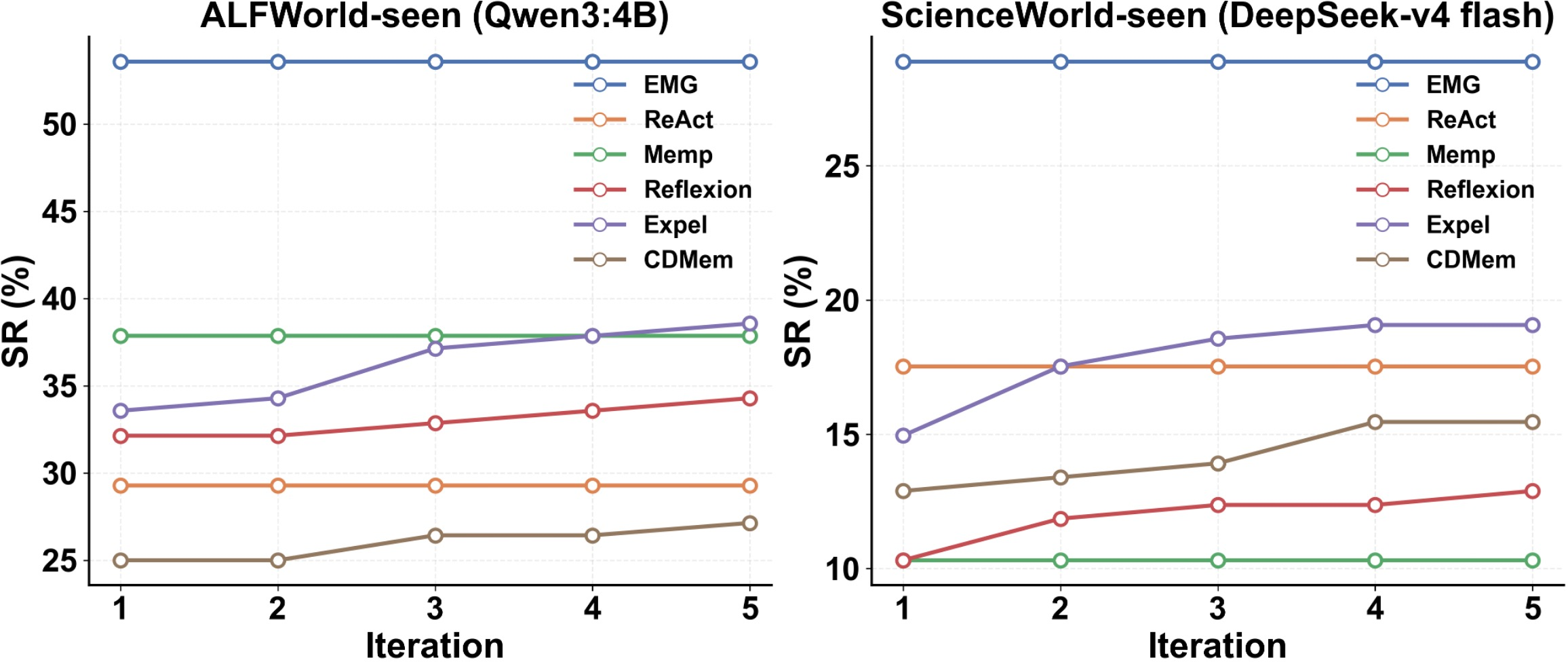
We evaluate all methods on the seen splits of ALFWorld (with Qwen3-4B) and ScienceWorld (with DeepSeek-V4-Flash). For iterative baselines (Reflexion, ExpeL, CDMem), we allow up to five test-time iterations and report their final success rate. For one-shot memory, they perform a single execution per test task without online trial-and-error. The results are shown in figure 3.
The results show that while some iterative baselines (e.g., Reflexion, ExpeL) can surpass simple one‑shot methods like ReAct or MemP after several rounds of reflection, our one‑shot EMG consistently achieves the highest success rate among all methods on both benchmarks. For instance, on ALFWorld with Qwen3-4B, the iterative success rates range from 27.14% to 38.57%, whereas EMG reaches 53.57% with a single execution. Similarly, on ScienceWorld with DeepSeek-V4-Flash, the iterative results vary between 12.89% and 19.07%, while EMG attains 28.87%. This demonstrates that our offline‑structured memory not only provides more effective correction than online trial‑and‑error loops, but also eliminates the need for multiple test‑time attempts, thereby significantly reducing both time and API costs.
5.5 Time Cost Comparison↩︎
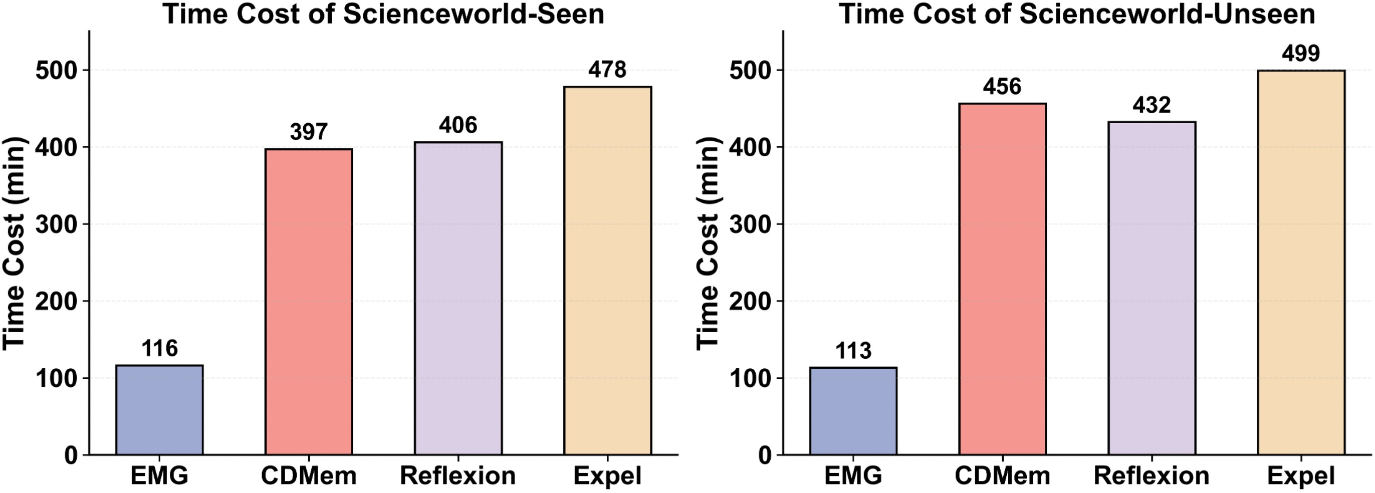
We evaluate the inference time efficiency of our EMG against iterative baselines (CDMem, Reflexion, ExpeL) on ScienceWorld using the Qwen3-4B model, as shown in figure 4. While iterative methods require up to five test‑time attempts to self‑correct, EMG performs only a single execution per task, leveraging offline‑constructed memory. As a result, EMG incurs substantially lower total inference time than all baselines, while simultaneously achieving higher success rates (see main results). The time advantage of EMG is consistent across both seen and unseen splits. Notably, when deployed with larger closed‑source models (e.g., DeepSeek-V4-Flash), the inference cost per attempt is considerably higher; EMG’s one‑shot nature therefore multiplies the savings in both time and API expenses, further underscoring its practical efficiency.
5.6 Hyperparameter Sensitivity Analysis↩︎
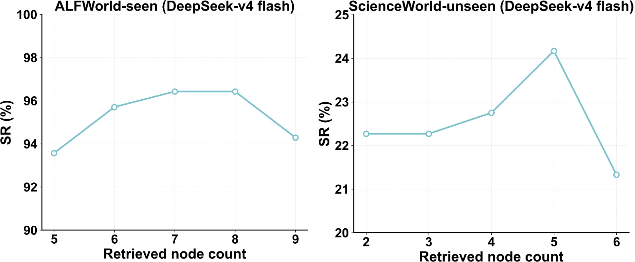
We analyze the sensitivity of EMG to the number of retrieved nodes (top‑\(k\)) on two benchmarks: ALFWorld seen and ScienceWorld unseen, both using DeepSeek-V4-Flash. On ALFWorld, we vary top‑\(k\) from 5 to 9; on ScienceWorld, we vary it from 2 to 6. Each node includes all of its connected edge insights for the retrieved memory, and we report the success rate as shown in figure 5.
Overall, EMG exhibits strong robustness across the tested range of \(k\). Performance remains consistently high with only minor fluctuations, and even the smallest retrieval sets achieve competitive results, indicating that the stored insights are highly informative and do not require many examples to be effective. A slight decline is observed when \(k\) becomes too large, which may be due to the inclusion of too many examples that occasionally distract the model in selecting the most appropriate correction. Nevertheless, the variation is modest, confirming that EMG is not sensitive to the exact choice of \(k\) and performs reliably without extensive tuning.
6 Conclusion↩︎
We propose Experience Memory Graph (EMG), a framework that constructs structured experience memory from training trajectories via graph matching. Unlike iterative self‑reflection methods that rely on costly test‑time trial‑and‑error, EMG formulates error correction as finding the shortest graph edit path between a failed exploration trajectory and a successful expert trajectory. By converting trajectories into directed action decision graphs and applying graph matching offline, we extract common subgraphs (successful workflows) and graph edit paths (correction instructions). These insights are organized into a memory graph where nodes store intra‑task knowledge and edges store cross‑task generalizable patterns, enabling one‑shot test‑time guidance without repeated loops. Experiments on extensive datasets demonstrate that EMG consistently outperforms strong iterative baselines in success rate and average reward, while requiring only a single test‑time attempt. Ablation and sensitivity studies confirm the effectiveness and robustness of the proposed model. For future work, we plan to extend EMG to environments without expert trajectories.
7 Details for constructing action decision graph↩︎
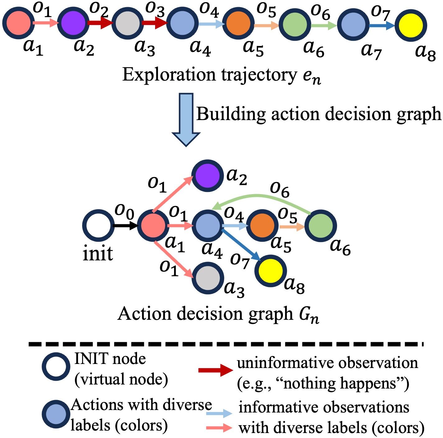

Algorithm 7 details the procedure of constructing the directed action decision graph. Figure 6 demonstrates a concrete example of how to transform the sequential raw exploration trajectory \(e_n\) into directed action decision graph \(G_n\), where \(o_i\) represents observations and \(a_i\) represents actions.
In the raw trajectory \(e_n\), observations \(o_2\) and \(o_3\) are uninformative (e.g., “nothing happened” in ALFWorld), indicating that actions \(a_2\) and \(a_3\) are both invalid attempts under the same valid observation \(o_1\). The subsequent action \(a_4\) is a valid action also taken under \(o_1\). If we directly applied graph edit distance to the raw sequential trajectory, we would delete \(o_2, o_3, a_2, a_3\); however, as \(o_2\) and \(o_3\) carry no meaningful information, the resulting edit path would produce an insight such as “under observation \(o_2\) do not take \(a_3\)”, which is meaningless. The correct insight should be “under observation \(o_1\), avoid \(a_2\) and \(a_3\)”. To capture this, we introduce parallelizing consecutive invalid actions: all actions that follow the same valid state \(o_1\) without changing the environment are connected in parallel from the same previous valid node. Hence \(a_2\), \(a_3\), and \(a_4\) all receive edges from \(a_1\) with the same edge label \(o_1\). This makes the graph edit path directly indicate which actions are invalid under \(o_1\).
Additionally, we observe that the same core action may be taken under different observations. To better model this, we propose node reuse: if a normalized action appears later in the trajectory (e.g., \(a_7\) is the same action as \(a_4\)), we do not create a new node; instead, we connect the incoming edge (carrying \(o_6\)) directly to the existing node of that action (\(a_4\)). This allows a single node to collect multiple incoming edges with different observation labels, revealing under which conditions that action is appropriate.
8 Algorithm of extracting common subgraph and graph edit path↩︎
Given a node matching \(M\) between two directed labeled graphs \(G\) and \(G'\) (obtained via the FGW solver), the following two algorithms extract structured knowledge from the matched graphs.
Algorithm 8 constructs the common subgraph by retaining only those edges in \(G\) whose both endpoints are matched and whose corresponding edge exists in \(G'\) with an identical edge label. This yields the set of actions that are already correct under the same observation, i.e., the successful workflow.
Algorithm 9 derives a complete graph edit path from \(M\). It collects unmatched nodes (deletions from \(G\) and insertions from \(G'\)), node label mismatches (relabelings), and edge mismatches (missing edges, extra edges, or label differences) to produce edge deletions, insertions, and relabelings. All collected operations together form a legal edit path that transforms \(G\) into \(G'\). Unlike classical methods designed for undirected graphs without edge labels, our algorithms explicitly handle directed edges and edge labels, preserving the semantic information carried by observations.

9 Discussion about the robustness of graph edit path↩︎
We further analyze the robustness of our graph edit path extraction (Algorithm 9). The overall graph matching procedure relies on the FGWAlign solver [36], which may not always produce the globally optimal node correspondence. According to the original FGWAlign evaluation, for graph pairs with tens of nodes, the recall of the predicted edit path against the ground‑truth shortest path is around 90%. It is important to clarify that a recall below 100% does not imply an invalid edit path. Given any node matching \(M\) (optimal or suboptimal), Algorithm 9 always generates a legal edit path: applying the returned insertions, deletions, and relabelings to the source graph \(G\) exactly yields the target graph \(G'\). The only difference is that a suboptimal matching may lead to a longer path (i.e., more edit operations) than the shortest possible one. Recall measures how many of the operations in the shortest path are preserved in our derived path; the remaining operations are legitimate but redundant alternatives.
Consequently, our method is highly robust to matching inaccuracies. Even when the node matching is not optimal, the extracted correction instructions remain valid and can successfully repair the failed trajectory. In the extreme (and practically improbable) case where the node matching is completely wrong — for instance, every node in \(G\) is matched to an unrelated node in \(G'\) — Algorithm 9 will produce an edit path that essentially deletes all actions of the failed trajectory and inserts (or relabels) all actions of the expert trajectory. The resulting insight reduces to “follow the successful trajectory entirely”, which, although not leveraging partial correctness, still provides a correct and executable plan. Hence, even under the worst possible matching, our framework offers a safe fallback. This robustness, together with the high empirical recall of the matching solver, guarantees that EMG reliably produces useful correction knowledge across a wide range of scenarios.
10 Notations↩︎
| Symbol | Meaning |
|---|---|
| \(\tau\) | Complete trajectory \((q, o_0, a_1, o_1, \dots, a_m, o_m)\) |
| \(q\) | Task query / instruction |
| \(a_t\) | Action at step \(t\) |
| \(o_t\) | Observation at step \(t\) |
| \(r\) | Reward (success/failure) |
| \(G = (V, E, q, r)\) | Action decision graph |
| \(v_i\) | Node in action decision graph (represents an action) |
| \(e_i\) | Edge in action decision graph, connecting \((v_i, v_{i+1})\) |
| \(\ell_n(v_i)\) | Node label (integer) |
| \(\ell_e(e_i)\) | Edge label (integer) |
| \(v_{\text{init}}\) | Virtual INIT node (\(\ell_n=0\)) |
| \(\mathcal{G}_m = (\mathcal{V}, \mathcal{E})\) | Experience Memory Graph |
| \(\nu_i\) | Node in experience memory graph (one training task) |
| \(\epsilon_{ij}\) | Edge in experience memory graph, connecting \(\nu_i\) and \(\nu_j\) |
| \(I_i^{\text{intra}}\) | Intra-task insight on node \(\nu_i\) |
| \(I_{ij}^{\text{cross}}\) | Cross-task insight on edge \(\epsilon_{ij}\) |
| \(G_i\) | Exploration graph for task \(i\) |
| \(G_i^*\) | Expert graph for task \(i\) |
| \(G_i^c\) | Common subgraph (successful workflow) |
| \(G_i^e\) | Graph edit path (correction instructions) |
| \(G_{ij}^c\) | Cross-task common subgraph |
| \(P\) | Node matching matrix |
| \(\pi\) | Soft assignment matrix (optimal transport) |