Online Random Sampling with Real Probabilities
July 15, 2026
Abstract
We develop an efficient online algorithm to sample a sequence of discrete random variables using an entropy source of i.i.d. fair coin flips, in a standard model of real computation where real-valued probabilities are represented by rational approximations. For any sequence \(F_1, F_2, \dots\) of probability distributions, our algorithm generates \(n\) outputs \(X_1 \sim F_1, \dots, X_n \sim F_n\) using at most \(\expect{H(F_1) +\dots + H(F_n)} + O(\log n)\) coin flips in expectation while carrying \(O(\log n)\) bits of persistent space, where \(H\) is the Shannon entropy. Under standard assumptions, we prove that our algorithm achieves this information-theoretically optimal entropy rate using asymptotically optimal space.
The key idea is to replace the global arithmetic-decoding sampling scheme of [1] ([1]) with a local discrete uniform state, yielding an exponential reduction in space for a given entropy loss. Our approach applies to distributions with irrational probabilities and countably infinite supports, generalizing recent randomness-recycling methods beyond finite rational distributions with bounded denominator.
1 Introduction↩︎
A fundamental problem in theoretical and applied computer science is to convert a sequence of random symbols drawn from an “input” stream into a sequence of random symbols that form the “output” stream. In random sampling, the input stream is a sequence \(B_1, B_2, \dots\) of i.i.d. fair coin flips and the output stream is a sequence \(X_1, X_2, \dots\) of random variables [2]. This operation is used in almost all computer simulations, such as algorithms for stochastic optimization or numerical integration that demand many random variables drawn from a dynamic sequence of target distributions.
The most flexible workflow for applications is online random sampling, where each target distribution \(F_i\) for \(X_i\) is revealed at stage \(i\) of a sampling loop, as shown in the following high-level pseudocode.
Input: Sequence \(B_1, B_2, \dots\) of i.i.d. coin flips Receive target distribution \(F\) Emit random variable \(X \sim F\)
At iteration \(i\) of the sampling loop, the algorithm must produce exact samples \(X_i \sim F_i\), even if conditioned on previous outputs \(X_1,\ldots,X_{i-1}\). The total number of requests may not be known in advance and may be unbounded. The algorithm may maintain some private internal state from round-to-round, and the rule for selecting each \(F_i\) must be independent of this private state conditioned on \(X_1, \ldots, X_{i-1}\).
Any algorithm that converts input coin tosses to other output variables typically incurs a loss of information, which is a direct consequence of the data processing inequality. More specifically, the Shannon entropy contained in the output variables is at most that of the consumed input coin flips. For example, consider rolling a fair six-sided die by first flipping three fair coins and then applying the mapping \[\set*{000 \mapsto 1, \quad 001 \mapsto 2, \quad 010 \mapsto 3, \quad 011 \mapsto 4, \quad 100 \mapsto 5, \quad 101 \mapsto 6, \quad 110 \mapsto R, \quad 111 \mapsto R},\] where 110 and 111 invoke a “reject and repeat” loop. It takes 4/3 trials to halt on average and each trial uses 3 bits of entropy, for a total of 4 input bits. The output roll carries \(\lg 6\) bits of entropy, so the expected entropy loss is \(4 - \lg 6 \approx 1.4150\) bits. A more efficient algorithm is to recycle an unused bit when rejecting: \[\set*{000 \mapsto 1, \quad 001 \mapsto 2, \quad 010 \mapsto 3, \quad 011 \mapsto 4, \quad 100 \mapsto 5, \quad 101 \mapsto 6, \quad 110 \mapsto R0, \quad 111 \mapsto R1}.\]
After rejecting with \(110\) or \(111\), the final bit can be reused, so that the next loop iteration only needs to draw two fresh bits. Now only \(11/3\) input flips are used on average, which saves 1/3 bit. As millions or even billions of outputs are generated, small differences in entropy consumption can accumulate into large differences in runtime. This overhead is most prominent in applications where the entropy source is expensive, such as cryptographic protocols requiring high-quality random bits [3]. We thus view the entropy loss as a fundamental quantity to be minimized, along with space and runtime.
1.0.0.1 Entropy Cost.
Formally, the \(n\)-step entropy loss of an online random sampling algorithm is the difference between the expected Shannon entropy of the input coin flips and the output symbols: \[\begin{align} L_n \coloneq\expect{ T_n - \sum_{i=1}^n H(F_i) } \ge 0 && (n \ge 1), \label{eq:entropy-loss} \end{align}\tag{1}\] where \(T_n\) is the random number of coin flips (each carrying 1 bit of information) used to produce the \(n\) outputs and \(H(F) \coloneq-\sum_{i} f(i) \lg f(i)\) is the Shannon entropy of a discrete cumulative distribution function (CDF) \(F\) with probability mass function (PMF) \(f(i) \coloneq F(i) - F(i-1)\). We aim to minimize \(\expect{T_n}\), and thus \(L_n\), while retaining efficient space and runtime.
1.0.0.2 Real-Valued Probabilities.
Many random sampling algorithms assume the Real RAM model. For example, the standard treatment in the statistical literature—where random sampling is often called “random variate generation”—assumes that arithmetic operations on real numbers take \(O(1)\) time [4]. In this setting, it is trivial to achieve \(L_n < 3\) via arithmetic decoding of the input bit stream [1], nearly matching the optimal entropy loss \(L_n < 2\) given in [2].
We aim to develop algorithms that handle distributions with arbitrary (irrational) probabilities in a more realistic model of computation than Real RAM. Following the standard model [5], we access each target distribution \(F\) via an approximation oracle \(\phi\) for its CDF, such that \(\abs{F(x) - \phi(x,k)} < 2^{-k}\) for any \(x,k \in \mathbb{N}\coloneq\set{0, 1, \dots }\). This assumption captures the usual situation for many practical distributions, where probabilities are not necessarily rational but can be computed to any prescribed precision.
In our setting, efficient sampling becomes significantly more challenging than “dice rolling” (i.e., sampling a finite-support distribution with rational probabilities), because there are now two sources of uncertainty
the infinitely precise uniform random real \(U \in [0,1]\), whose bits \(B_1, B_2, \dots\) are presented as the i.i.d. coin flips from the entropy source; and
the cumulative probabilities \(F(x)\) in the target distribution, which are real numbers known up to finite precision after a finite number of oracle queries.
An efficient sampling algorithm must carefully balance the cost of drawing fresh coin flips from the entropy source with the cost of invoking the oracle at higher and higher precision to control the space, time, and entropy costs.
1.0.0.3 Space Cost.
We distinguish persistent space, which is the number of bits used for the state persisting between the iterations of online sampling, and temporary space, which is used only within a single sampling iteration. The overall space is the maximum of these two quantities across all iterations of online sampling. If the distributions have irrational probabilities, then the temporary space must be unbounded to guarantee exact outputs, although the expected temporary space may remain bounded. On the other hand, there is no restriction on the persistent space: it is zero for algorithms that waste entropy by maintaining no state, and it grows unbounded as \(n \to \infty\) for classical algorithms achieving (near) optimal entropy loss [1], [2].
1.0.0.4 Global State for Online Random Sampling.
The dice-rolling example illustrates a general phenomenon: reducing entropy loss requires preserving randomness that was not fully used by the sampler. More generally, if a sampler for a CDF \(F\) outputs \(X=x\) using \(U \sim \mathrm{Unif}[0,1]\), then the conditional position of \(U\) inside the interval \([F(x-1),F(x)]\) remains uniform. This information constitutes “unused” randomness that can be used in future sampling rounds to reduce the number of fresh bits drawn from the entropy source.
A key obstacle to efficient online sampling is that existing methods reduce entropy cost by storing reusable randomness from the entire output history. In online sampling with arithmetic decoding [1], the reusable randomness is maintained globally, by carrying a high-precision interval containing \(U\) after producing \(n\) outputs \(X_1, \dots, X_n\). For example, if all the probabilities are rationals with denominator \(d\), then endpoints have a denominator growing as \(d^n\), and the expected space is \(O(n)\).
1.0.0.5 Key Idea: Local Randomness Recycling.
Instead of storing a large global interval as in arithmetic coding, we maintain a local discrete state which is a lossy, compressed form of the unused randomness from the previous samples. Specifically, after each step \(i\), our sampler’s state is a pair of integers \((Z_{i}, M_{i})\) with \(Z_{i} \mid M_{i} \sim \mathrm{Unif}\set{0,\dots,M_{i}-1}\). We sample \(X_{i+1}\) using a uniform variate \(Q_{i+1}\) constructed from \((Z_{i}, M_{i})\) and fresh coin flips from the source as needed. Then, a new uniform state \((Z_{i+1}, M_{i+1})\) is obtained by compactly encoding the relative position of \(Q_{i+1}\) within the interval \([F_{i+1}(x_{i+1}-1),F_{i+1}(x_{i+1})]\).
The state is not obtained by simply truncating high-precision interval endpoints, which introduces bias. Instead, we use a discrete re-encoding that preserves exactness while bounding the state size. To control the space, we set an upper bound \(M_i \leq \Delta_i\) that evolves with the iteration count \(i\). Choosing the sequence \(\Delta_i\) is a delicate balance: larger values give a lower asymptotic entropy loss but increase the runtime. Large values also create leftover randomness that is discarded at the (unknown) end of the online sampling procedure.
In our algorithm, we choose \(\Delta_i\) to scale as \(i \log i\) up to some optional specified maximum value, after which it stabilizes. Over \(n\) rounds, the entropy loss is \(L_n \leq \epsilon n + O(\log n)\) and the persistent space is \(O(\log \min\set{1/\epsilon, n})\), which is an exponential improvement over the global-state approach. Here \(\epsilon\) can be any desired user-specified parameter, including \(\epsilon = 0\) to obtain a purely logarithmic entropy loss.
1.0.0.6 Overview of the Algorithm.
1 gives an overview of the randomness-recycling procedure.
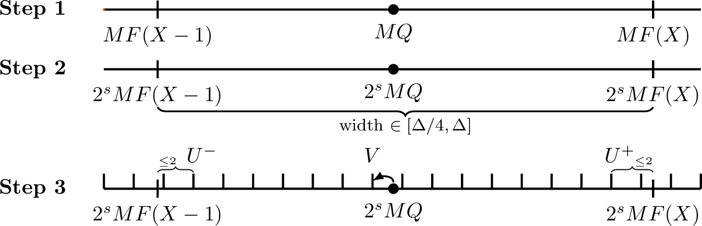
Conditioned on generating \(X \sim F\) at a given round, the conditional distribution of the uniform variate \(Q \sim \mathrm{Unif}[0,1]\) becomes \(Q \mid X \sim \mathrm{Unif}[F(X-1), F(X)]\). We will extract a new state \((Z', M')\) that captures unused randomness from the most recent sampling round.
We first scale the interval \([F(X-1), F(X)]\) by \(M 2^s\), where \(s\) is chosen to give an interval width \(2^sM ( F(X) - F(X-1) ) \in [\Delta/4, \Delta]\) (1, Step 2), which implies that \[(2^sMQ \mid X, M) \sim \mathrm{Unif}[2^sMF(X-1), 2^sMF(X)]. \label{eq:rhinoscopy}\tag{2}\]
We next compute integer points \(U^-\) and \(U^+\) such that the interval \(\set{ U^-, U^- + 1, \dots, U^+ -1}\) is strictly contained in the real interval \([2^s MF(X-1), 2^sMF(X)]\), with a small gap at the endpoints. 2 implies that the floor \(V \coloneq\floor{2^sMQ}\) is uniformly distributed over \(\set{U^-, \dots, U^+-1}\) conditioned on falling in this set (1, Step 3, blue region). In this case, we extract \(Z' \coloneq V - U^-\) and \(M' \coloneq U^+-U^-\) as a new discrete state \((Z',M')\), with \(Z' \mid M' \sim \mathrm{Unif}\set{0,\dots,M'-1}\) and \(M' \leq \Delta\) as desired. The factor \(2^s M\) is key to efficiently performing these computations given rational-approximation access to \(F\) and bit access to \(Q\).
1.1 Main Results↩︎
Equipped with this background, a high-level summary of our main result is as follows.
Theorem 1 (Informal). For every online sequence of discrete distributions with computable-real CDF access, exact online sampling can be performed with \(O(\log n)\) total entropy loss after \(n\) samples while storing only \(O(\log n)\) bits of persistent state. Under standard assumptions, the sampler has polynomial expected running time per sample and \(O(\log n)\) expected overall space over \(n\) samples. The logarithmic overall-space bound is optimal up to constant factors in the CDF-oracle model.
A more formal description of the results is as follows.
Theorem 2 (Simplified). There is an online random sampling algorithm that, given CDF oracles for target distributions \(F_1, \dots, F_n\), outputs \(X_1 \sim F_1, X_2 \sim F_2, \dots\) with entropy loss \(L_n \leq O(\log n)\), such that when sampling \(X_i\) at iteration \(i\),
The persistent space is \(O(\log i)\) bits;
The expected temporary space is \(O(\log i + \expect{\log X_i})\) bits;
The expected number of calls to the CDF oracle is \(O(\expect{\log X_i})\);
The expected number of arithmetic operations is \(O(\expect{\log X_i})\), and the expected bit lengths of the relevant operands are \(O(\log i +\expect{\log X_i})\);
For efficient CDF oracles (according to the standard notions in 4 5 ), the expected running time is within a constant factor of the expected cost of \(\log X_i\) invocations of the oracle at \(X_i\) with \(\lg X_i\) bits of precision, plus one invocation of the oracle at \(X_i\) with \(\lg i\) bits of precision.
Our method can also interpolate between entropy loss \(L_n \leq O(\log n)\)—with space and runtime per sample scaling as \(\log{n}\), as stated in 2—and entropy loss \(L_n \leq \epsilon n + o_\epsilon(n)\)—with space and runtime per sample scaling as \(\log(1/\epsilon)\)—yielding a spectrum of trade-offs between entropy loss and space. In the latter configuration, the \(\log(1/\epsilon)\) persistent space is asymptotically optimal, matching the lower bound shown in [6]. We further show in 7 that the expected overall space is essentially optimal, up to constant factors. The proposed method improves on existing algorithms as follows.
The interval algorithm of [1] uses exponentially more persistent and temporary space than our algorithm to achieve a given entropy loss, as made precise in ¿tbl:table:compare-interval?. Their algorithm also requires querying the previous CDFs with increasing precision, while our algorithm does not.
The algorithm in [7] (for i.i.d. outputs) generates batched samples, with entropy loss \(L_n \leq \epsilon n + o_\epsilon(n)\) using \(O(1/\epsilon)\) persistent space. Our algorithm uses \(O(\log(1/\epsilon))\) space and can support full online random sampling with non-i.i.d. outputs. The algorithms are compared in ¿tbl:table:compare-kozen?.
The algorithms in [8] assume distributions with rational probabilities having denominator bounded by \(d\), while our algorithm supports countably many symbols and arbitrary real probabilities. Further, [8] achieve \(L_n \leq \epsilon n + o_\epsilon(n)\) using \(O(\log(d/\epsilon))\) space while our algorithm uses \(O(\log(1/\epsilon))\), removing the dependence on the denominator size.
2 Related Work↩︎
As a starting point, [2] first described entropy-optimal online sampling, with entropy loss satisfying \(L_n < 2\) for every \(n\). This method presupposes effective access to the bits in the binary expansions of the output probabilities (and the joint probabilities via cumulative products), which is possible in the Real RAM model but incompatible with the standard model of computable reals. In particular, access to binary expansions is not computably admissible [5] because carries may propagate indefinitely, so basic arithmetic operations such as addition cannot be implemented bitwise.
2.0.0.1 [9]
study online generation of discrete random variates from a finite set of \(N\) dynamically changing rational weights, with total weight \(S\). The data structures support sampling and weight updates in a transdichotomous RAM model with constant-time arithmetic on \(O(\log S)\)-bit quantities. In their model, the entropy source emits a uniform integer in \(\set{0,\ldots,S-1}\) in \(O(1)\) time; they do not track entropy cost in terms of individual coin flips. This setting is similar to ours in its dynamic nature but is otherwise orthogonal in its model and objectives: [9] target dynamically changing fixed-precision distributions over finite support without regard to entropy loss, while we study entropy-efficient sampling from infinite-support distributions with CDFs accessed through rational approximation oracles.
2.0.0.2 [1]
describe a method of arithmetic coding called the interval algorithm for online random sampling. It also handles uniform and nonuniform input and output streams, subject to an arbitrary dependence structure. As with our method, it also supports various configurations of the space–entropy tradeoff. ¿tbl:table:compare-interval? compares the two methods under different choices of parameters.
max width=
Our method requires exponentially less space to achieve entropy loss \(L_n \leq \epsilon n + o_\epsilon(n)\), as \(\epsilon\) decreases. Furthermore, our algorithm can achieve logarithmic space and logarithmic entropy loss, compared to the linear space and constant entropy loss with the default iterative approach from [1]. Note that the persistent space bound of 4 is deterministic while the bound [1] holds only in expectation.
2.0.0.3 [8]
describe a general online random sampling technique for reducing entropy loss when the output distributions are over a finite domain and have rational probabilities with denominator bounded by \(d\). It achieves entropy loss \(L_n \leq \epsilon n + O(\log(d/\epsilon))\) for any \(\epsilon > 0\) using \(O(\log(d/\epsilon))\) persistent and temporary space. Randomness recycling is shown to accelerate [10]’s alias method [10], inversion and lookup-table sampling [4], DDG tree sampling [2], [11]–[13], and batched uniform sampling [14], [15]. Applying this method to arbitrary discrete distributions requires each target distribution to be decomposed as a series of bounded rational distributions, as in [7]. However, this decomposition is inefficient in general, requiring a linear scan over the probabilities, with expected time at least linear in the mean of the distribution. Our algorithm instead manipulates the CDF oracles directly, allowing logarithmic dependence on the mean via binary search, while maintaining the same entropy efficiency via a carefully optimized randomness-recycling procedure. Thus, we generalize and improve on [8], eliminating the dependence on \(d\) and efficiently handling arbitrary distributions.
2.0.0.4 [7]
discuss an algorithm to produce i.i.d. outputs in batches, trading off persistent space (i.e., the batch size) with entropy loss. We improve on [7] in two ways. First, our method handles a dynamic sequence of non-i.i.d. target distributions, while the batching method used by [7] only works for an i.i.d.output sequence from a fixed distribution. Second, even for i.i.d. outputs, our sampling algorithm achieves an exponential improvement in space. ¿tbl:table:compare-kozen? gives the full comparison, showing how the \(1/\epsilon\) overall expected space required by batching in [7] is reduced to \(\log(1/\epsilon)\) space using the randomness-recycling method in this work.
max width=
2.0.0.5 Other Algorithms.
Several exact sampling algorithms for specific distributions have been developed, e.g. for the geometric [16], the Laplace and Gaussian [17], [18], the Bernoulli [19], and exponential [20]. These methods are tailored to particular distributions and do not aim to conserve entropy or support online random sampling from dynamic sequences of distributions.
[21] present arbitrary-precision algorithms for discrete and continuous distributions. To reduce entropy cost of sampling, they leverage the interval method [1] to recycle coin flips, although it is applied in a way that does not guarantee correct outputs [8].
Another direction is exact sampling given a floating-point approximation to a CDF [22]–[24]. Algorithms to minimize the statistical distance between a finite discrete distribution with irrational probabilities and a finite rational approximation are given in [25] using the \(\ell_1\) distance and KL divergence, and in [26] more generally using any \(f\)-divergence.
2.0.0.6 Complexity Theory.
[27] develop a probabilistic Turing machine model for random sampling with bounded (as opposed to expected) polynomial time, and study the problem of efficiently simulating output dice with as few different types of biased input coins as possible. [28] studies the relationship between computable distributions and polynomial-time approximate samplability up to a small error. Our oracle model is similar in that the real-valued target probabilities are accessed via rational approximations. However, we take computable-real access as the input representation and ask for exact online sampling with near-optimal entropy consumption, explicit oracle-cost bounds, and small space.
[29] present various time and space complexity bounds in the Real RAM for sampling a finite discrete distribution given unnormalized probabilities \((p_1, \dots, p_n) \in \mathbb{R}^n_{\ge 0}\). In this setting, entropy cost is not a traceable aspect of the complexity analysis, because a uniform real in \([0,1]\)—which has infinitely many random bits—can also be obtained and manipulated in \(O(1)\) time.
3 Computational Model↩︎
3.0.0.1 Notation.
We write \(\ln x\) and \(\lg x\) for the usual natural logarithm and base-two logarithm respectively. Further, we define \(\log x \coloneq\ln \max\set{ x, e} \geq 1\) for \(x \geq 0\).
3.0.0.2 Word RAM Arithmetic.
Throughout this paper, we assume a word size of \(w \ge 1\) bits and define \(W \coloneq 2^w\). Basic word operations (e.g., addition, subtraction, division, multiplication) take \(O(1)\) time. A big integer \(z\) is stored as a sequence \((z_{k-1}, \dots, z_0)\) of \(w\)-bit limbs representing \(z = z_{k-1}W^{k-1} + \dots + z_1 W^1 + z_0\). From \(z\) we can form a new integer \(z' \coloneq z_{k-1}W^{k'-1} + \dots + z_{k-k'}\) by copying the top \(k' \le k\) limbs in \(O(k')\) time. A rational number is stored as a pair \((z,y)\) of integers representing \(z/y\). Addition and subtraction on big integers take \(k = O(\log_W N)\) word operations. Other operations are more expensive. For instance, multiplication and division take \(O(k \log k)\) time using the method of [30], or \(\Theta(k^2)\) using the schoolbook method (see [31] for a comprehensive overview).
From a practical standpoint, this model aligns with existing CPU designs with registers of size \(w = 64\). From a theoretical standpoint, it avoids tracking the bit complexity of low-level operations. One important consequence of our representation for big integers is that it allows sublinear-time operations. The following result will be useful for our algorithm.
There is an algorithm \(\Call{ApproxDivision}{q,k}\) that takes as input a rational number \(q = a/b \in [0,1]\) and integer \(k \ge 1\), and returns in \(O(k)\) time a rational number \(q' = a'/b'\) such that \(\abs{q - q'} < 2^{-k}\), where \(0 \le a' \le b' < 2^{k+1}\) (i.e., \(a'\) and \(b'\) each have bit length at most \(k+1\)).
Proof. See 8. ◻
3.0.0.3 Representing Probability Distributions.
We consider probability distributions with support \(\mathbb{N}\). A CDF \(F: \mathbb{N}\to \mathbb{R}\) is a nondecreasing function with \(F(0) \geq 0\) and \(\lim_{i \to \infty} F(i)=1\). The corresponding PMF is given by \(f(i) \coloneq F(i) - F(i-1)\) for \(i \geq 0\), where by convention we write \(F(-1) \coloneq 0\).
An oracle for \(F\) is a function \(\phi: \mathbb{N}\times \mathbb{N}\to \mathbb{Q}\) such that \(\abs{F(i) - \phi(i,k)} < 2^{-k}\), and \(\phi(i,k)\) has denominator \(2^{k}\) for every \(i,k\). We also define \(\phi(-1,k) \coloneq 0\) for all \(k\).
We define the bound oracles \[\begin{align} \Fl{i}{k} \coloneq\phi(i,k+1) - 2^{-(k+1)} \qquad \text{and} \qquad \Fu{i}{k} \coloneq\phi(i,k+1) + 2^{-(k+1)}, \end{align}\] which satisfy \[\begin{align} \Fl{i}{k} < F(i) < \Fu{i}{k} \qquad \text{and} \qquad \Fu{i}{k} - \Fl{i}{k} \leq 2^{-k}. \label{hrup5} \end{align}\tag{3}\]
To account for the cost of evaluating the oracle, we define \(\CF{x}{\nu}\): \(x \geq 0, \nu \geq 1\) to be an upper bound on the number of word-level operations needed to evaluate the oracle \(\phi(i',k')\) over all \(i' \leq \ceil{x}\), \(k' \leq \ceil{\lg \nu} + 1\), and we suppose that \(\mathcal{C}_F\) is nondecreasing in \(x\) and \(\nu\). We say the oracle is accuracy efficient /index efficient if there is a polynomial \(g\) with \[\begin{align} &\bfseries \underline{accuracy efficient} & \frac{\CF{x}{\nu'}}{\CF{x}{\nu}} &\le g\!\left( \frac{\log \nu'}{\log \nu} \right) & (x \geq 0; 1 \leq \nu < \nu'), \tag{4} \\ &\bfseries \underline{index efficient} & \frac{\CF{x'}{\nu}}{\CF{x}{\nu}} &\le g\!\left( \frac{\log x' }{\log x} \right) & (\nu \geq 1; 0 \leq x < x'). \tag{5} \end{align}\] An oracle for \(F\) is efficient if it is both accuracy-efficient and index-efficient. Many distributions have efficient oracles; for instance, the Poisson distribution (via algorithms to estimate the incomplete Gamma functions [32]) or the discretized Gaussian distribution (via algorithms to estimate the error function [33]).
When dealing with efficient oracles, all the asymptotic notations may have a hidden dependence on the polynomial \(g\) in 4 5 . The intent is that, for a certain genre of oracle (e.g. oracles for Gaussians), the terms in \(g\) would be small fixed constants. To avoid edge cases in the analysis, we set \(\CF{x}{\nu} \coloneq\CF{x}{1}\) for \(\nu < 1\), and we assume that \(\CF{x}{\nu}\) is at least as large as the cost of basic arithmetic operations on quantities of magnitude \(\ceil{x}\) and \(\nu\). This convention ensures that the cost of computing \(F^{\pm}(i,k)\) is \(O\!\left(\CF{i}{2^k}\right)\) for \(k \geq 0\).
The next result establishes the cost of estimating the PMF given a CDF oracle.
There is an algorithm \(\Call{EstimatePMF}{F, x, \nu}\) that takes a CDF \(F\), an integer \(x \geq 0\), and an integer \(\nu \geq 1\), and returns an estimate \(\hat{p}\) of the probability mass \(p \coloneq f(x)\) such that \(\hat{p} \le p \le (1+1/\nu) \hat{p}\), with runtime \(O\!\left( \log(\nu/p)\thinspace \CF{x}{8 \nu/p} \right).\) (If \(p = 0\), the algorithm runs forever without returning any output).
Proof. See 9. ◻
4 Online Random Sampling: Overview↩︎
As a starting point, 2 shows a simple, stateless procedure for random sampling. It is based on the [1] interval method adapted to the case that the target CDF is given via an oracle.
![Figure 2: Online random sampling using the (stateless) [1] interval method.](/article/2607.13828/_pdflatex/ylhqopwz.png "fig:")
This sampling algorithm performs a dichotomous search over \(\mathbb{N}\) to find the value \(X\) with \(Q \in [F(X-1), F(X)]\) where \(Q \sim \mathrm{Unif}[0,1]\) is an infinitely precise real that is known to lie in the interval \([\hat{Q}, \hat{Q} + 2^{-r}]\). The oracle for \(F\) is queried at the current midpoint \(X^{\text{mid}}\) with \(r\) bits of precision. If \(\hat{Q}\) is to the right of the upper bound, we recurse right. If \(\hat{Q} + 2^{-r}\) is to the left of the lower bound, we recurse left. If neither condition holds, then a fresh bit is sampled to narrow the interval containing \(Q\).
2 returns a sample from distribution \(F\), and it uses \(H(F) + O(1)\) random bits in expectation. Moreover, if \(F\) is efficient, then the expected runtime is \[O\!\left(\expect{ \log(X) \thinspace \CF{X}{X} } \right).\]
Proof. This is a direct corollary of the analysis in 5 for the special case \(\Delta=M=1\), where 2 and 4 are essentially equivalent. ◻
While 2 is efficient in runtime, it wastes significant entropy. In the remainder of this paper, we present our novel online random sampling method. The basic plan, given in 3, is to repeatedly call a method (4). The method generates a single variable \(X\) given a CDF \(F\) using i.i.d. coin flips; it additionally consumes and produces a discrete uniform random state \((Z,M)\) of recycled randomness, where \(Z \mid M \sim \mathrm{Unif}\set{0,\dots,M-1}\) and \(M \leq \Delta\).
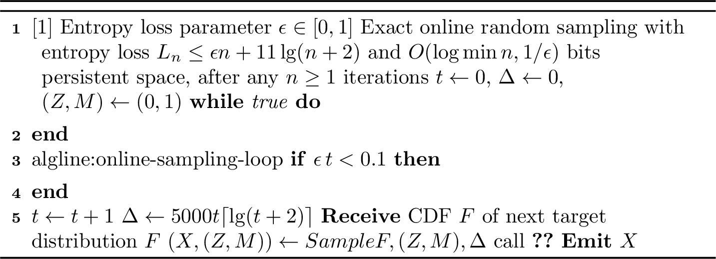
With this parametrization, the values after each iteration \(k\) satisfy \[0 \le Z < M \leq \Delta \leq \mathop{\mathrm{poly}}(t) \leq \mathop{\mathrm{poly}}( \min\set{1/\epsilon, k} ).\]
The total persistent space to store the global state of 3 is therefore \(O\!\left(\log \min\set{1/\epsilon, k} \right)\). We will establish the following main result.
Theorem 3 (store=entropy-bound-overall,restate-keys=note=Restated). The entropy loss \(L_n\) after \(n\) iterations of the sampling loop in 3 satisfies \[L_n \leq \epsilon n + 11 \lg(n+2).\]
4 provides the main individual sampling procedure . This procedure – in particular, the subroutine – implements the rule described previously in 1. We describe in 5, and analyze the sampling loop from 3 in 6.

5 Single Variable Sampling with Uniform Random States↩︎
Here \(\Delta \ge M\) is an integer parameter dictating the size of the output state. We will analyze the call \[(X, (Z', M')) \leftarrow \Call{Sample}{F,(Z,M),\Delta}.\]
Fix \(M\), and suppose that \(Z \sim\mathrm{Unif}\set{0, \dots, M-1}\) and \(B \coloneq(B_1, B_2, \dots)\) is an infinite sequence of random bits from the entropy source. Then the following quantity is uniformly distributed over \([0,1]\): \[Q = \frac{Z + \sum_{i=1}^{\infty} B_i 2^{-i}}{M}. \label{eq:q-uniform}\tag{6}\]
begins by calling \(\Call{IntervalSample}{F,(Z,M)}\), which uses the randomness in \(Z\) to extend the baseline method \(\Call{IntervalSampleStateless}{F}\). The call to returns a sample \(X \sim F\) as well as the random bits \((B_1, \dots, B_r)\) used to generate the outcome. The interval \([\hat{Q}, \hat{Q} + 2^{-t+1}]\) approximates the real quantity \(Q\). Next, the call to attempts to recycle the used random bits into a new random state \((Z', M')\), which may require fresh random bits to obtain a wide enough discrete interval around \(Q\).
The following invariants hold in each iteration of : \[\begin{align} r=\max &\set{0,t-\floor{\lg M}}, \tag{7} \\ \hat{Q} \leq{} & Q \leq \hat{Q}+2^{-t+1}, \tag{8} \\ F(X^--1) \leq{} & Q \leq F(X^+). \tag{9} \end{align}\]
Proof. We show 7 by induction on \(t\). The base case holds since \(t = r = 0\) and \(M \geq 1\). For the induction step, if the new value has \(t < 1 + \lfloor \lg M \rfloor\), then \(t - \lfloor \lg M \rfloor \leq 0\) and \(r\) remains zero. If the new value has \(t \geq 1 + \lfloor \lg M \rfloor\), then both \(t\) and \(r\) increment, while \(t - \lfloor \lg M \rfloor\) also increments and is strictly positive.
For 8 , there are two cases. Suppose \(r > 0\) and \(\hat{Q}\) is derived at [qform1]. So \(\hat{Q} \leq Q \leq \hat{Q} + 2^{-r}/M\), as the missing bits \(B_{r+1}, \dots\) can contribute at most \(2^{-r}\) in total. By 7 , we have \(2^{-r}/M = 2^{-t + \lfloor \lg M \rfloor} / M \leq 2^{-t} \leq 2^{-t+1}\). Otherwise, suppose \(r = 0\) and \(\hat{Q}\) is derived at [qform2]. Then we have \(Z/M \leq Q \leq (Z+1)/M\). By the specification of , we have \(Z/M - 2^{-t} \leq \hat{Q} \leq Z/M\) and \(Q - \hat{Q} \leq (Z+1)/M - (Z/M - 2^{-t}) \leq 1/M + 2^{-t}\). Since \(r = 0\), we have \(t \leq \lfloor \lg M \rfloor\) and so \(1/M \leq 2^{-t}\).
For 9 , first note that \(F(-1) = 0 \leq Q \leq 1 = F(\infty)\) initially. Next, observe that if \(X^-\) updates to \(X^{\text{mid}}+1\), then by 8 we have \(F(X^{\text{mid}}) \leq \Fu{X^{\text{mid}}}{t} \leq \hat{Q} \leq Q\). So \(F(X^-- 1) \leq Q\). Similarly, if \(X^+\) updates to \(X^{\text{mid}}\), then by 8 we have \(Q \leq \hat{Q} + 2^{-t+1} \leq \Fl{X^{\text{mid}}}{t} \leq F(X^{\text{mid}})\). ◻
The following invariants hold for \(\Call{Recycle}{F, (Z,M), \Delta, X, (B_1, \dots, B_r)}\): \[\begin{align} \Delta/4 \leq & 2^s M f(X) & \leq \Delta \tag{10} \\ 2^s M F(X) - 2 \leq & U^+ & \leq 2^s M F(X) \tag{11} \\ 2^s M F(X-1) \leq & U^- & \leq 2^s M F(X-1) + 2 \tag{12} \\ V \leq & 2^s M Q & \leq V + 1. \tag{13} \end{align}\]
Proof. By specification of , we have \(\hat{p} \leq f(X) \leq 2 \hat{p}\).
The bounds 10 hold from the specification of \(\hat{p}\), the definition of \(s\), and our hypothesis that \(M \leq \Delta\).
The bounds 11 hold because \[\frac{U^+}{2^s M} \leq \Fl{X}{s + \ceil{\lg M}} \leq F(X) \leq \Fl{X}{s + \ceil{\lg M}} + \frac{1}{2^s M} \leq \frac{U^+ + 2}{2^s M}.\] The bounds 12 are completely analogous.
The bounds 13 hold since \(2^s M Q - V = 2^s \sum_{i=s+1}^{\infty}B_i 2^{-i}\) and \(0 \leq 2^s \sum_{i=s+1}^{\infty}B_i 2^{-i} \leq 1\). ◻
The sampled value \(X\) is the unique index with \(Q \in [F(X-1),F(X)]\) (aside from the probability-zero event that \(Q\) equals a CDF boundary), and \(X\) is \(F\)-distributed. Moreover, if we condition on the event \(\set{X = x}\) for any \(x\) with \(f(x) > 0\), then \(Q\) is uniformly drawn from the range \([F(x-1), F(x)]\).
Proof. Because \(X^-= X^+= X\) at termination, we have \(Q \in [F(X-1), F(X)]\) by [obs:interval-sample-invariants]. Because \(Q\) is uniformly distributed in \([0,1]\), \(\Pr(X = x) = \Pr(Q \in [F(x-1), F(x)]) = f(x)\), and \(Q\) is uniform in \([F(x-1), F(x)]\) conditioned on \(X = x\). ◻
The recycled values \((Z', M')\) satisfy \(0 \leq Z' < M' \leq \Delta\) always. Furthermore, conditioned on the values of \(X\), \(M\), and \(M'\), the output \(Z'\) is uniformly distributed over \(\set{0, \dots, M' - 1}\).
Proof. When we condition on \(M\) and \(X = x\), the values \(s\), \(U^-\), and \(U^+\) are completely determined, because \(F\) is a deterministic oracle.
The results are trivial if \(M' = 1\), so consider the case with \(U^- \leq V < U^+\) and \(M'=U^+-U^-\). Here, from [prop:recycling-integer-bounds], we have \(U^+ - U^- \leq 2^s M F(X) - 2^s M F(X-1) = 2^s M f(X) \leq \Delta\). Furthermore, for any choice of variables \((Z, B_1, \dots, B_s)\) which satisfy \(U^- \leq V < U^+\), we have \(Q \in [F(x-1), F(x)]\) and thus \(X = x\). Therefore, all such values of \((Z, B_1, \dots, B_s)\) will still have a uniform distribution conditioned on \(X = x\); in particular, \(V - U^-\) is uniform in the range \(\set{0, \dots, U^+ - U^- - 1}\). ◻
Let \(k \geq 0\). The final value of the variable \(t\) in \(\Call{IntervalSample}{F, (Z,M)}\) satisfies \[\Pr\left( t > k \mid X, M\right) \leq \frac{6}{2^k f(X)}.\]
Proof. Consider the iteration \(t=k\) just before \(t\) increments to \(k+1\). As neither of the conditions modifying \(X^-\) or \(X^+\) held then, we have \[\Fl{X^{\text{mid}}}{t} - 2^{-t+1} \leq \hat{Q} \leq \Fu{X^{\text{mid}}}{t}\]
As \(\Fu{X^{\text{mid}}}{t} \leq F(X^{\text{mid}}) + 2^{-t}\) and \(\Fl{X^{\text{mid}}}{t} \geq F(X^{\text{mid}}) - 2^{-t}\), we have \[\label{eq:fa1} \hat{Q} - 2^{-t} \leq F(X^{\text{mid}}) \leq \hat{Q} + 3 \cdot 2^{-t}.\tag{14}\]
Putting together 14 8 gives \[\label{eq:q1r} Q - a \leq F(X^{\text{mid}}) \leq Q + a \qquad \text{where a = 3 \cdot 2^{-k}}\tag{15}\]
Now suppose we condition on \(X = x\). If \(X^{\text{mid}}\geq x\), then 15 implies that \(Q \geq F(X^{\text{mid}}) - a \geq F(x) - a\); likewise if \(X^{\text{mid}}< x\) then 15 implies that \(Q \leq F(X^{\text{mid}}) + a \leq F(x-1) + a\). Putting the two cases together, we conclude that \[\label{eq:q2r} Q \in \left[ F(x-1), F(x-1) + a \right] \cup \left[F(x) - a, F(x) \right].\tag{16}\]
By , the probability that 16 holds conditional on \(X = x\) is at most \(\frac{2 a}{f(x)}\). ◻
5.1 Analysis of Entropy Loss↩︎
Theorem 4. If \(\Delta \geq 1000\), then the total number of sampled bits \(T \coloneq\max\set{r, s}\) in [algline:online-sampling-bit1] [algline:online-sampling-bit2] of 4 satisfies \[\expect{T - \lg M' \mid M, X} \leq \lg(1/f(X)) - \lg M + \frac{48 \lg \Delta}{\Delta}.\]
Proof. Conditioned on \(X = x\), the value \(s\) is a constant while \(r\) remains a random variable. We have \[\expect{T- \lg M' \mid M, X } = \left( s + \sum_{k=s}^{\infty} \Pr( r > k) \right) - \left( \Pr\left( U^- \leq V < U^+\right) \lg\left(U^+ - U^-\right) \right).\]
Let \(\theta \coloneq 2^s M f(x)\). By 7 and [prop:precision-geometric-tail], we have \[\begin{align} \sum_{k=s}^{\infty} \Pr( r > k ) = \sum_{k=s}^{\infty} \Pr( t > k + \lfloor \lg M \rfloor) \leq \sum_{k = s}^{\infty} \frac{6}{2^{k + \lfloor \lg M \rfloor} f(x)} = \frac{12}{2^{s + \floor{\lg M}} f(x)} \leq \frac{24}{\theta}. \end{align}\]
Next, the bound 13 implies that \[\begin{align} \Pr ( U^- \leq V < U^+ \mid X ) = \frac{U^+ - U^-}{2^s M f(x)} = \frac{U^+ - U^-}{\theta}. \end{align}\]
By 11 and 12 we have \(U^+ - U^- \geq \theta - 4\), so overall \[\begin{align} \expect{T - \lg M' \mid M, X} &\leq s + \frac{24}{\theta} - \left( 1 - \frac{4}{\theta} \right) \lg( \theta - 4) = s - \lg \theta + \frac{24}{\theta} - \lg (1 - 4/\theta) + \frac{4}{\theta} \lg (\theta-4) \end{align}\]
Here, \(s - \lg \theta = \lg(1/f(x)) - \lg M\). Note that \(\theta\ge \Delta/4\ge 250\). Using this fact and straightforward calculations, we get \[\label{eq:xccs1} \frac{24}{\theta} - \lg \left(1 - \frac{4}{\theta}\right) + \frac{4}{\theta} \lg (\theta - 4) \leq \frac{12 \lg \theta}{\theta} \le \frac{48\lg\Delta}{\Delta}. \qedhere\tag{17}\] ◻
5.2 Analysis of Complexity↩︎
Conditioned on \(X = x\), the expected runtime of is \[O\!\left(\CF{x}{\Delta/p} + \log( x+1/p) \sum_{i=0}^{\infty} 2^{-i} \CF{2x}{2^i/p} \right) \qquad \text{for p = f(x)}.\]
Proof. In the phases of where \(X^+= \infty\), we always have \(X^-\leq x\); in each such iteration, we set \(X^{\text{mid}}= 2 X^-\leq 2 x\). We can only modify \(X^-\) this way \(O(\log x)\) times. Then, after \(X^+< \infty\), each iteration that modified \(X^+\) or \(X^-\) will reduce \(X^+-X^-\) by a constant factor. Again, such iterations can occur only \(O(\log x)\) times. Overall, \(X^{\text{mid}}\) takes \(O(\log x)\) different values, all of which are at most \(2 x\).
We claim that each iteration of has cost \(O(\CF{2x}{2^{t}})\). Indeed, if \(r = 0\), then the numerator and denominator of \(\hat{Q}\) are \(\mathop{\mathrm{poly}}(2^t)\), and we query \(F^{\pm}(X^{\text{mid}}, t)\), so the arithmetic is performed on values of magnitude polynomial in \(2^t\). Even though \((Z, M)\) may have bit length \(O(\log \Delta)\), we avoid any dependence on \(\Delta\) via [prop:approx-div]. If \(r > 0\), then \(M < 2^t\) and again the arithmetic is performed on values of size \(2^t M \leq \mathop{\mathrm{poly}}(2^t)\).
Let \(t_0 = \lfloor \lg 1/p \rfloor\). There are at most \(O( t_0 + \log x) = O(\log(x + 1/p))\) iterations with \(t \leq t_0\), since in each iteration either \(X^{\text{mid}}\) or \(t\) is updated; each such iteration has cost \(O(\CF{2x}{2^t}) \leq O(\CF{2x}{1/p})\). So the total cost of all such iterations is at most \[\label{bar1} O\!\left( \log(x+1/p) \thinspace \CF{2x}{1/p}\right).\tag{18}\]
Likewise, for \(i > 0\), there are at most \(O(\log x)\) iterations with \(t = t_0 + i\), and the cost of each such iteration is \(O(\CF{2x}{2^i/p})\). By [prop:precision-geometric-tail], the probability of reaching such value \(t\) is at most \(1/(2^t p) \leq O( 2^{-i} )\). So the total contribution from these iterations is at most \[\label{bar2} O\left( \log(x) \thinspace 2^{-i} \CF{2x}{2^i/p} \right)\tag{19}\]
The contributions from 18 and 19 , summed over all \(i > 0\), together can be bounded as \[\label{bar3} O \Bigl( \log(x+1/p) \thinspace \sum_{i=0}^{\infty} 2^{-i} \CF{2 x}{2^i/p} \Bigr).\tag{20}\]
In , the call has cost \(O(\log (1/p) \thinspace \CF{x}{8/p})\), which is within a constant factor of 20 . The arithmetic for \(U^-\) and \(U^+\) and oracle queries for \(F(x-1)\) and \(F(x)\) have cost \(O(\CF{x}{\Delta/p})\). ◻
Theorem 5. Suppose the oracle is accuracy efficient. Conditioned on \(X = x\), the expected runtime of \(\Call{Sample}{F, (Z,M), \Delta}\) is \[O \left(\CF{x}{\Delta} + \log( x+1/p) \thinspace \CF{2x}{1/p} \right) \qquad \text{for p = f(x)}.\]
Proof. By [prop:runtime-conditional-general], the expected runtime, ignoring constant factors, is given by \[\CF{x}{\Delta/p } + \log( x+1/p) \sum_{i=0}^{\infty} 2^{-i} \thinspace \CF{2x}{2^i/ p}.\]
Using our assumption on \(\cal C_F\), we can bound the sum \(\sum_{i=0}^{\infty} 2^{-i} \thinspace \CF{2x}{2^i/ p}\) by \[\begin{align} O(\CF{2x}{1/p}) \sum_{i=0}^{\infty} 2^{-i} g\!\left(\frac{\log(2^i/p)}{\log(1/p)}\right) \leq O(\CF{2x}{1/p}) \sum_{i=0}^{\infty} 2^{-i} g(i+1) \leq O(\CF{2x}{1/p}) \end{align}\] using the polynomial \(g\) from 4 . We can also bound \[\begin{align} \CF{x}{\Delta/p} &\leq \CF{x}{1/p^2} + \CF{x}{\Delta^2} \leq \CF{x}{1/p} g\!\left(\frac{\log(1/p^2)}{\log(1/p)}\right) + \CF{x}{\Delta} g\!\left(\frac{\log(\Delta^2)}{\log(\Delta)}\right) \\ &\leq O(\CF{x}{1/p} + \CF{x}{\Delta}). \end{align}\]
The term \(\CF{x}{1/p}\) is dominated by the other term \(\CF{2x}{1/p}\) appearing in the stated bound. ◻
Theorem 6. If the oracle is efficient, then the expected runtime of \(\Call{Sample}{F, (Z,M), \Delta}\) is \[O \Bigl( \expect[X \sim F]{ \CF{X}{\Delta} + \log (X) \thinspace \CF{X}{X} } \Bigr).\]
Proof. By 5, the expected runtime is, up to constant factors, given by \[\begin{align} \expect{\CF{X}{\Delta}} + \expect{\log(X+1/f(X)) \thinspace \CF{2 X}{1/f(X)}}, \end{align}\] where \(X\) follows the distribution \(F\). Consider the function \[h(x,y) = \CF{x}{\Delta} + \log(x+y)\thinspace \CF{2 x}{y}.\] It can be seen that this function satisfies the condition \[\begin{align} \frac{h(x,y)}{h(x',y')} \leq C\!\left( \frac{\log x \log y}{\log x' \log y'} \right)^k && (0 \leq x' \leq x, 0 \le y' \leq y) \end{align}\] for some constants \(C, k\). As we show in 3 from 10, such a function satisfies \[\expect{h(X, 1/f(X))} \leq O(\expect{h(X, X)})\] Here \(h(X, X) \leq O( \CF{X}{\Delta} + \log(X) \thinspace \CF{X}{X})\). ◻
Corollary 1. Let \(\mu = \expect{X}\). If the oracle is efficient, then \(\Call{Sample}{F, (Z,M), \Delta}\) has expected runtime \[O \Bigl( \CF{\mu}{\Delta} + \log(\mu) \thinspace \CF{\mu}{\mu} \Bigr).\]
Proof. By monotonicity and efficiency, for every \(x \in \mathbb{N}\) we have \[\log(x) \thinspace \CF{x}{x} \le \log(\mu) \thinspace \CF{\mu}{\mu} \thinspace g(x), \qquad g(x) \coloneq C\!\left(1+\left(\frac{\log x}{\log\mu}\right)^k \right).\]
It remains to show that \(\expect{g(X)}=O(1)\). By our definition of the \(\log\) function and Jensen’s inequality, \[\log^k x \leq \log^k\left(x + e^k\right) \implies \expect{\log^k X} \le \expect{\log^k\left(X + e^k\right)} \le \log^k\left(\mu + e^k\right) = O\!\left(\log^k \mu\right).\] Therefore \(\expect{g(X)}=O(1)\). The same argument, without the leading factor \(\log x\), applies to \(\CF{x}{\Delta}\). The claim follows from 6. ◻
Let \(S\) denote the temporary space of \(\Call{Sample}{F, (Z,M), \Delta}\). Conditioned on \(X\), there is some constant \(c\) with \[\Pr( S \geq c \log (X + \Delta/f(X)) + \lambda \mid X) \leq O( 2^{-\lambda})\] for all \(\lambda \geq 1\). In particular, \[\expect{S \mid X} \leq O( \log(X + \Delta/f(X)) ).\]
Proof. The space of is \(O(t + \log (X + \Delta))\), and the space of is \(O(\log(\Delta / f(X)))\). By [prop:precision-geometric-tail], conditioned on \(X\), the final value of \(t\) has mean at most \(O(\log(1/f(X)))\), with the tail bounded by a geometric distribution. ◻
6 Online Random Sampling Analysis↩︎
We are now prepared to analyze the main sampling loop of 3. We index iterations of the loop in 3 starting from \(i=1\); each iteration \(i\) receives \(F_i\), starts from state \((Z_{i-1},M_{i-1})\), calls with parameter \(\Delta_i\), and returns \(X_i\) together with the new state \((Z_i,M_i)\). We set \((Z_0,M_0) \coloneq(0,1)\).
For every \(n\), the entropy loss after the first \(n\) iterations of 3 satisfies \[L_n \le \lg\Delta_n + 48\sum_{i=1}^n \frac{\lg\Delta_i}{\Delta_i}.\]
Proof. Let \(T_i\) denote the number of sampled bits in iteration \(i\). Suppose we condition on all random variables \(X_1, \dots, X_{i-1}, M_1, \dots, M_{i-1}\), as well as any external randomness determining the distributions \(F_1, \dots, F_i\). Then \(Z_{i-1} \sim \mathrm{Unif}\set{0,\dots, M_{i-1}-1}\). By 4 there holds \[\expect{T_i - H(F_i) + \lg(M_{i-1}/M_i)} \leq \frac{48 \lg \Delta_i}{\Delta_i}.\]
Summing over \(i = 1, \dots, n\) and using iterated expectations, the unconditioned expectation satisfies \[\begin{align} L_n + \expect{\lg(M_0/M_n)} = \expect{\sum_{i=1}^n \left( T_i - H(F_i) + \lg(M_{i-1}/M_i) \right) } \leq 48 \sum_{i=1}^n \frac{\lg \Delta_i}{\Delta_i}. \end{align}\]
Since \(M_0 = 1\), we have \(\mathbb{E}[\lg(M_0/M_n)] = -\mathbb{E}[\lg M_n]\), so \[L_n \le \expect{\lg M_n} + 48\sum_{i=1}^n \frac{\lg\Delta_i}{\Delta_i} \le \lg\Delta_n + 48\sum_{i=1}^n \frac{\lg\Delta_i}{\Delta_i},\] where the last inequality uses \(M_n \le \Delta_n\). ◻
Proof. Let \(m \coloneq\ceil{0.1/\epsilon}\) (infinite if \(\epsilon = 0\)). Thus the value of \(\Delta\) used in iteration \(i\) is \[\Delta_i = D_{\min\{i,m\}}, \qquad \text{ for } D_j \coloneq 5000j\lceil \lg(j+2)\rceil \quad (j\ge 1).\] It is readily verified that \[\lg D_j \le 10\lg(j+2) \quadand\quad 48\thinspace \frac{\lg D_j}{D_j} \le \frac{0.1}{j}. \label{eq:mnestic}\tag{21}\]
By [prop:entropy-loss], we have \[L_n \le \lg\Delta_n + 48\left[ \sum_{i=1}^{\min \{ n,m \}} \frac{\lg\Delta_i}{\Delta_i} + \sum_{i=m+1}^n \frac{\lg\Delta_m}{\Delta_m} \right].\] Since \(\Delta_n=D_{\min\set{n,m}}\), the first bound in 21 gives \[\lg\Delta_n \le 10\lg(n+2).\] For the summation, applying the second bound in 21 to the increasing part of the summation gives \[48 \thinspace \sum_{i=1}^{\min\set{n,m}} \frac{\lg\Delta_i}{\Delta_i} < 0.1\sum_{i=1}^{\min\{n,m\}}\frac{1}{i} \le 0.1(1+\ln n) \le \lg(n+2).\] Finally, if \(n>m\), applying the second bound in 21 with \(j = m\) and \(0.1/m \le \epsilon\) gives \[48\sum_{i=m+1}^n \frac{\lg\Delta_m}{\Delta_m} \le (n-m)\thinspace 48 \thinspace \frac{\lg\Delta_m}{\Delta_m} \le (n-m)\thinspace \frac{0.1}{m} \le (n-m) \epsilon \le \epsilon n.\] Combining the three bounds indeed gives \[L_n \le 10\lg(n+2)+\lg(n+2)+\epsilon n \le \epsilon n+11\lg(n+2). \qedhere\] ◻
Corollary 2.
Suppose that the oracle family is uniformly efficient, i.e., that all the oracles \(F_i\) use a single upper-bound cost function \(\CF[F]{\cdot}{\cdot}\) which satisfies 5 4 . If there exists a finite deterministic value \(\mu_n\) such that \(\expect{X_i \mid F_i} \le \mu_n\) \((1\le i\le n)\) a.s., then the expected runtime over \(n\) iterations of the sampling loop in 3 is \[O\!\left( n \thinspace \CF{\mu_n}{\min\set{n, 1/\epsilon}} + (n \log \mu_n) \thinspace \CF{\mu_n}{\mu_n} \right).\]
Proof. Sum the bounds from 1 over all iterations \(i = 1, \dots, n\), using the fact that \(\Delta_i\) is nondecreasing. Since the oracles are efficient, we have \(\CF{\mu_n}{\Delta_i} \leq O( \CF{\mu_n}{\min\set{i,1/\epsilon}} )\). ◻
If there exists a finite deterministic value \(\mu_n\) such that \(\expect{X_i \mid F_i} \le \mu_n\) \((1\le i\le n)\) a.s., then the expected overall space usage over \(n\) iterations of the sampling loop in 3 is \(O(\log n+\log\mu_n)\).
Proof. Let \(p_i = f_i(X_i)\) where \(f_i\) is the PMF of \(F_i\). Let \(S_i\) represent the space usage of iteration \(i\) of the sampling loop, and let \(S_{1:n} \coloneq\max_{1 \le i \le n} S_i\). If we condition on \(F_i\) and \(X_i\), then [prop:sgeomtail] gives \[\Pr \left( S_i \geq \lambda + c \log(X_i + \Delta_i/p_i) \mid F_i, X_i \right) \leq O( 2^{-\lambda} ).\]
By a union bound over the indices \(i = 1, \dots, n\), and the fact that \(\log \Delta_i \leq O( \log n)\) for each \(i\), we have \[\expect{S_{1:n}} \leq O\!\left( \log n + \expect{\max_{1 \le i \le n} \log X_i} + \expect{\max_{1 \le i \le n} \log(1/p_i)} \right).\]
Now consider an iteration \(i\), and suppose we condition on the distribution \(F_i\). By Markov’s inequality, \[\Pr\left( \ln X_i \geq t + \ln \mu_n \mid F_i \right) = \Pr\left( X_i \geq e^{t} \mu_n \mid F_i \right) \leq e^{-t}.\] By a union bound, we have \(\Pr(\max_i \ln X_i \geq t+\ln \mu_n) \leq n e^{-t}\), and hence again \[\expect{\max_{1 \le i \le n} \log X_i} \leq O(\log n + \log \mu_n).\]
Similarly, as we show in 4, we have \(\Pr \left( \log(1/p_i) \geq t + 3 \log (\mu_n + 3) \mid F_i \right) \leq e^{-t/3}\), and hence by completely analogous arguments \[\expect{ \max_{1 \le i \le n} \log(1/p_i) } \leq O(\log n + \log \mu_n). \qedhere\] ◻
7 Space Lower Bound↩︎
Here, we show that the overall space usage of any online sampler accessing target distributions via CDF oracles must grow as \(\Omega(\log n + \expect{\max_{1 \le i \le n} \log X_i})\). By [prop:space-bound-overall], our algorithm matches this lower bound provided that \(\mu_n \le \mathop{\mathrm{poly}}(n)\), in which case it is optimal up to constant factors.
To establish the result, we first prove a useful lemma which states that determining \(F(0)\) up to \(k\) bits of precision requires oracle calls \(\phi(i,j)\) with \(j \geq k - 1\).
Lemma 1. Let \(F\) be any distribution with a CDF oracle \(\phi\), and let \(k\in\mathbb{N}\). There exist rational numbers \(a, b\) with \(b-a\ge 2^{-k}\) such that, for each \(c\in(a,b)\), there is a distribution \(G\) with \(G(0)=c\) and a CDF oracle \(\psi\) agreeing with \(\phi\) on all queries with precision parameter at most \(k\).
Proof. Define \[a \coloneq\max\bigl(\set{0} \cup \set{\phi(0,j)-2^{-j}:0\le j\le k}\bigr), \qquad b\coloneq\min\bigl(\set{1} \cup \set{\phi(i,j)+2^{-j}:i\in\mathbb{N},\;0\le j\le k}\bigr).\] These extrema are well defined: for \(0\le j\le k\), the oracle values \(\phi(i,j)\) have denominator \(2^j\) and lie in a bounded interval, so only finitely many values can appear in the displayed sets. Moreover, all values appearing in the definitions of \(a\) and \(b\) are integer multiples of \(2^{-k}\).
The oracle guarantees give \(\phi(0,j)-2^{-j} < F(0) \leq F(i) < \phi(i,j)+2^{-j}\) for \(i \geq 0\). Thus, if \(F(0)\in(0,1)\), then \(a<F(0)<b\). If \(F(0)=0\), then \(a=0<b\), while if \(F(0)=1\), then \(a<1=b\). In all cases, \(a<b\). Since \(a\) and \(b\) are integer multiples of \(2^{-k}\), it follows that \(b-a\ge 2^{-k}\).
Now fix any \(c\in(a,b)\). Define a CDF \(G\) by \(G(0)\coloneq c\), and \(G(i)\coloneq\max\set{c,F(i)}\) for \(i\ge1\). This function is nondecreasing, satisfies \(G(-1)=0\), and has \(\lim_{i\to\infty}G(i)=1\), so it is a valid CDF on \(\mathbb{N}\). We define the oracle \(\psi\) for \(G\) as follows: for \(j \leq k\), we set \(\psi(i,j) = \phi(i,j)\) and for \(j > k\) we set \(\psi(i,j)\) to be a nearest dyadic rational with denominator \(2^j\). The oracle is clearly valid for \(j > k\). So consider a query \(\psi(i,j)\) with \(j \leq k\). For \(i=0\), since \(c\in(a,b)\), the definitions of \(a\) and \(b\) give \[\begin{align} \phi(0,j)-2^{-j}<c<\phi(0,j)+2^{-j} && (0\le j\le k), \end{align}\] and hence \(|\phi(0,j)-G(0)|<2^{-j}\). For \(i\ge1\), if \(G(i)=F(i)\), then validity follows from the oracle guarantee for \(F\). Otherwise \(G(i)=c>F(i)\), and for \(0\le j\le k\) we have \[\begin{align} \phi(i,j)-2^{-j}<F(i)<c<b\le \phi(i,j)+2^{-j}. \end{align}\] Thus \(\abs{\phi(i,j)-G(i)}<2^{-j}\) in this case as well. ◻
Lemma 2. Let \(\mathcal{S}\) be an exact online random sampling algorithm that accesses target distributions via CDF oracles. Let \(F_1,\ldots,F_n\) be arbitrary distributions on \(\mathbb{N}\), each equipped with a CDF oracle. For any \(k\in\mathbb{N}\), let \(E\) denote the event that \(\mathcal{S}\) makes no oracle queries with precision parameter above \(k\) during the first \(n\) sampling steps when run on \((F_1,\ldots,F_n)\). Then \(\Pr(E)\le (1-2^{-k})^n\).
Proof. For each \(i\), let \(a_i,b_i\) be the values from 1 applied to \(F_i\). Let \(X\coloneq(X_1,\ldots,X_n)\) be the outputs of \(\mathcal{S}\) when run on \((F_1,\ldots,F_n)\), and define the associated Bernoulli variables \(\widetilde{X}_i \coloneq\mathbf{1}_{\set{X_i>0}}\).
Fix any binary sequence \(z\coloneq(z_1,\ldots,z_n)\in\set{0,1}^n\). Let \(\delta\in(0,2^{-k-1})\), and define \[c_i \coloneq \begin{cases} a_i+\delta, & z_i=0,\\ b_i-\delta, & z_i=1. \end{cases}\] Here each \(c_i\in(a_i,b_i)\). Therefore, by 1, there is a distribution \(G_i\) with \(G_i(0)=c_i\) whose CDF oracle agrees with that of \(F_i\) on all queries with precision parameter at most \(k\).
Now consider coupled executions of \(\mathcal{S}\) on the oracles \((F_1,\ldots,F_n)\) and \((G_1,\ldots,G_n)\); let \(Y\coloneq(Y_1, \dots, Y_n)\) be the outputs in the run on \((G_1,\ldots,G_n)\), and set \(\widetilde{Y}_i \coloneq\mathbf{1}_{\set{Y_i>0}}\). On the event \(E\), the oracles for \(F_i\) and \(G_i\) agree on all queries made by \(\mathcal{S}\). So the two coupled executions have identical transcripts; in particular, \(E \implies X=Y \implies \widetilde{X} = \widetilde{Y}\). Therefore, \[\Pr\left(E \wedge \left(\widetilde{X}=z\right)\right) \le \Pr\left(\widetilde{Y}=z\right) = \prod_{i:z_i=0} c_i \prod_{i:z_i=1} (1-c_i) = \prod_{i:z_i=0} (a_i+\delta) \prod_{i:z_i=1} (1-b_i+\delta).\] Since this inequality holds for every \(\delta\in(0,2^{-k-1})\), letting \(\delta \rightarrow 0\) gives \[\Pr\left(E \wedge \left(\widetilde{X} = z\right)\right) \le \prod_{i:z_i=0} a_i \prod_{i:z_i=1} (1-b_i).\] Summing over \(z\in\set{0,1}^n\), we obtain \[\begin{align} \Pr(E) = \sum_{z\in\set{0,1}^n} \Pr\left(E\wedge\left(\widetilde{X} = z\right)\right) \le \sum_{z\in\set{0,1}^n} \prod_{i:z_i=0} a_i \prod_{i:z_i=1} (1-b_i) = \prod_{i=1}^n \bigl(a_i+1-b_i\bigr) \leq \left(1-2^{-k}\right)^n, \end{align}\] where the final inequality uses \(b_i-a_i\ge 2^{-k}\) for every \(i\). ◻
We state our main lower bound result:
Theorem 7. The expected overall space usage of any online sampling algorithm accessing the target distributions via CDF oracles grows over \(n\) iterations as \[\Omega\left(\log n + \expect{\max_{1 \leq i \leq n} \log X_i} \right).\]
Proof. For the dependence on \(X_i\), note that the (random) bit length of the output \(X_i\) is \(\Theta(\log X_i)\), and so the space usage over \(n\) iterations is at least \(\Omega(\expect{\max_{1 \leq i \leq n} \log X_i})\).
For the dependence on \(n\), note that by 2, any such sampling algorithm must make an oracle call with precision above \(k\) bits with probability at least \(1 - (1-2^{-k})^n\). In our model, such a query requires at least \(k\) bits of space to represent the answer. So the maximum space usage \(S\) over the \(n\) iterations satisfies \[\Pr(S \geq k) \geq 1 - \left(1-2^{-k}\right)^n\] for each \(k \in \mathbb{N}\), and \[\expect{S} \geq \sum_{k=1}^{\infty} \left( 1 - \left(1-2^{-k}\right)^n \right) \geq \Omega(\log n). \qedhere\] ◻
8 Algorithm ApproxDivision: Proof of↩︎
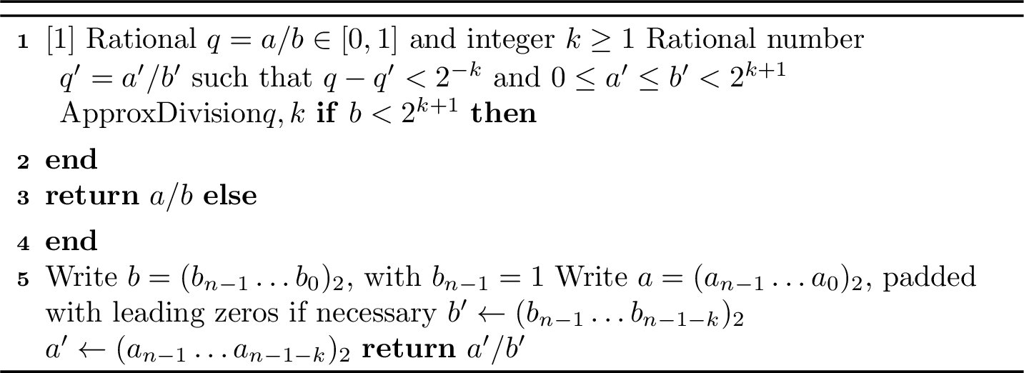
The case \(b < 2^{k+1}\) is clear. So suppose \(b \geq 2^{k+1}\) and let \(s \coloneq n-(k+1)\). Observe that \(b' = \floor{b/2^s} \ge 2^k\) and \(a' = \floor{a/2^s}\). Now write \[\begin{align} a = 2^s(a' + \alpha), \quad b = 2^s(b' + \beta), \end{align}\] for some \(0 \le \alpha, \beta < 1\). The bound \(\abs{a/b-a'/b'} < 2^{-k}\) follows immediately: \[\abs*{\frac{a}{b} - \frac{a'}{b'}} = \abs*{\frac{a' + \alpha}{b' + \beta} - \frac{a'}{b'}} = \frac{\abs*{b'\alpha - a'\beta}}{b'(b'+\beta)} < \frac{b'}{b'(b'+\beta)} < \frac{1}{b'+\beta} < \frac{1}{b'} \le \frac{1}{2^k},\] where the first inequality follows from the fact that \(0 \le a' \le b'\) and \(0 \le \alpha, \beta < 1\), so that \(\abs*{b'\alpha - a'\beta} < b'\).
By our assumption, the leading \(k+1\) bits of \(b\) and \(a\) lie in a consecutive block of at most \(\ceil{(k+1)/w}+1\) limbs, so the algorithm’s computational cost is \(O(\ceil{(k+1)/w}+1) = O(k)\).
9 Algorithm EstimatePMF: Proof of↩︎
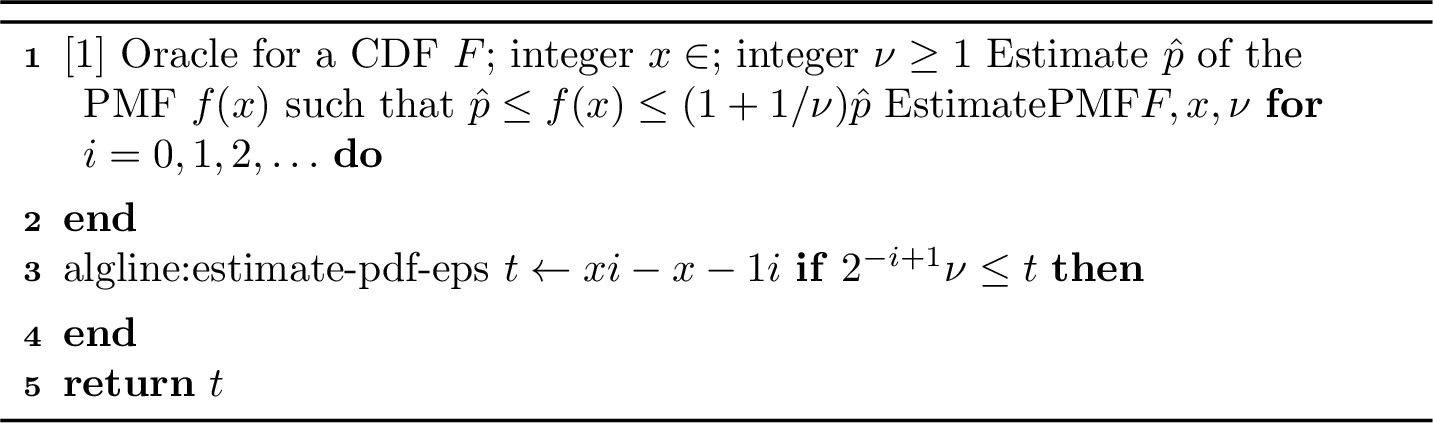
Let \(\hat{p} = t\) be the return value ([algline:estimate-pdf-retval]) at the final iteration \(i\). We first show that \(\hat{p} \le p \le (1+1/\nu) \hat{p}\). From the oracle bound, each iteration \(i\) satisfies \[\begin{align} p = F(x) - F(x-1) \ge \Fl{x}{i} - \Fu{x-1}{i} = t = \hat{p}, \end{align}\] which confirms the lower bound. Also, at the final iteration we have \[\begin{align} p & \le \Fu{x}{i} - \Fl{x-1}{i} = t + 2^{-i+1} \label{eq:ti-eq} \le (1 + 1/\nu) t, \end{align}\tag{22}\] where the last inequality follows from the halting condition \(t \geq 2^{-i+1} \nu\).
We next establish the runtime. At iteration \(i = i_{*} \coloneq\ceil{2 + \lg(\nu/p)}\), we have \[\begin{align} t \cdot 2^{i} &= 2^{i} \left( \Fl{x}{i} - \Fu{x-1}{i} \right) \geq 2^{i} (p - 2^{-i+1})= 2^{i} p - 2 \ge 4 \nu - 2 \geq 2 \nu \end{align}\] and so the algorithm terminates at this iteration or earlier. In each iteration, the oracle is invoked with inputs \((x, i+1)\) and \((x-1, i+1)\), where \(i \leq i_* \leq \lg(8 \nu/p)\). These use oracle inputs \(k \leq \lceil \lg(8 \nu/p) \rceil + 1\), as required by the definition of \(\CF{x}{8 \nu/p}\). The arithmetic costs are also less than a constant multiple of \(\mathcal{C}_F\).
10 Technical Lemmas↩︎
Lemma 3. Let \(h: \mathbb{R}_{\geq 0}^2 \rightarrow \mathbb{R}_{\geq 0}\) be any function which is nondecreasing in both arguments and for which there exist values \(C, k \geq 1\) with \[\begin{align} \label{eq:ff33} \frac{h(x,y)}{h(x',y')} \leq C \left( \frac{\log x \log y}{\log x' \log y'} \right)^k && (0 \leq x' \leq x, 0 \le y' \leq y) \end{align}\qquad{(1)}\]
Let \(a_0, a_1, \dots\) be nonnegative real numbers with \(\sum_i a_i = 1\). Then \[\sum_{i=0}^{\infty} a_i h ( i, 1/a_i ) \leq c \sum_{i=0}^{\infty} a_i h( i, i)\] for some factor \(c\) that depends on \(k\) and \(C\).
Proof. Throughout this proof, we regard \(C\) and \(k\) as constants; all asymptotic notations may depend on these parameters. Thus, applying ?? with \(x' = y' = 0\) and any values \(x, y \geq 0\) gives \[\label{eq:ff34} h(x,y) \leq O\!\left(h(0,0)\log^k x \log^k y\right).\tag{23}\]
Partition \(\mathbb{N}= A_1 \cup A_2 \cup A_3\), where \[\begin{align} A_1 = \set*{ i : i \leq e^{k} }, \qquad A_2 = \set*{i: i > e^{k}, a_i \geq (i+2)^{-2} }, \qquad A_3 = \set*{ i: i > e^{k}, a_i < (i+2)^{-2} }. \end{align}\]
Clearly, \(\abs{A_1} \leq \ceil{e^{k}} = O(1)\) and \(i \leq e^k \leq O(1)\) for \(i \in A_1\). Using 23 , the contribution of \(A_1\) is \[\begin{align} \label{eq:A1-bound} \sum_{i \in A_1} a_i h(i, 1/a_i) \leq O \Bigl( h(0,0)\sum_{i \in A_1} a_i \log^k i \log^{k}(1/a_i) \Bigr) \leq O \Bigl( h(0,0)\sum_{i \in A_1} a_i \log^{k}(1/a_i) \Bigr). \end{align}\tag{24}\]
The function \(x \mapsto x \log^k(1/x)\) is bounded above by \(\max\set{1,(k/e)^k}=O(1)\) on \([0,1]\). Hence, 24 is at most \[O(h(0,0)) \sum_{i \in A_1}1 = O( h(0,0)) |A_1| =O\!\left(h(0,0)\right).\]
Next consider the contribution of \(A_2\). Here, since \(h\) is nondecreasing in its second argument, we calculate \[\begin{align} \label{eq:nom1} \sum_{i \in A_2} a_i h(i, 1/a_i) \leq \sum_{i \in A_2} a_i h\left(i, (i+2)^2\right) \end{align}\tag{25}\]
Applying ?? with \(x = x' = i\), \(y = (i+2)^2\), and \(y' = i-2\), the right-hand side of 25 is at most \[O \Bigl( \sum_{i \in A_2} a_i h(i, i) \Bigr) \leq O \Bigl( \sum_{i=0}^{\infty} a_i h(i, i) \Bigr).\] Note here that \(i - 2> e^k - 2 > 0\) since \(i \in A_2\).
Finally, for the contribution to \(A_3\), we calculate \[\begin{align} \sum_{i \in A_3} a_i h(i, 1/a_i) \leq O \Bigl( h(0,0)\sum_{i \in A_3} a_i \log^k i\log^{k}(1/a_i) \Bigr). \end{align}\]
Consider again the function \(x \mapsto x \log^k(1/x)\). For \(x < e^{-k}\), it is increasing in \(x\). Here, \(a_i < e^{-k}\) and \(a_i < (i+2)^{-2} \leq (e^k + 2)^{-2}\) by definition of \(A_3\), so \[a_i \log^k(1/a_i) \leq (i+2)^{-2} \log^k\left((i+2)^2\right),\] and hence \[\begin{align} \sum_{i \in A_3} a_i h(i, 1/a_i) \leq O \Bigl( h(0,0)\sum_{i \in A_3} (i+2)^{-2}\log^{2k}(i+2) \Bigr) =O\!\left(h(0,0)\right). \end{align}\]
Because \(h\) is nondecreasing and \(\sum_i a_i=1\), we have \(h(0,0) \leq \sum_{i=0}^{\infty}a_i h(i,i)\). So putting the three cases together, we have \[\sum_{i=0}^{\infty} a_i h(i, 1/a_i) \leq O \Bigl( \sum_{i=0}^{\infty}a_i h(i,i) \Bigr). \qedhere\] ◻
Corollary 3. For any random variable \(X\) over \(\mathbb{N}\) with PMF \(f\), the Shannon entropy satisfies \[H(X) \coloneq\expect{\lg(1/f(X))} \leq O(\expect{\log X}). \qedhere\]
Proof. Apply 3 with function \(h(x,y) = \log y\) and \(k = 1\); here \(\expect{\log(1/f(X))} = \sum_i a_i h(i, 1/a_i)\) for \(a_i = f(i)\). So \(\expect{\log(1/f(X))} \leq O( \expect{ h(X, X) }) = O(\expect{\log X})\). ◻
Lemma 4. For any random variable \(X\) supported over \(\mathbb{N}\) with PMF \(f\) and mean \(\mu = \expect{X}\), there holds \[\Pr \left( \ln(1/f(X)) \geq t + 3 \ln (\mu + 3) \right) \leq e^{-t/3}.\]
Proof. Let \(Y \coloneq 1/f(X)\). Exponentiating and applying Markov’s inequality gives \[\Pr \bigl( \ln Y \geq t + 3 \ln (\mu + 3) \bigr) = \Pr \bigl( Y^{1/3} \geq e^{t/3} (\mu + 3) \bigr) \leq e^{-t/3} (\mu+3)^{-1} \expect{Y^{1/3}}.\]
Let \(a_i \coloneq f(i)\). We bound the expectation of \(Y^{1/3}\) as \[\begin{align} \expect{Y^{1/3}} &= \sum_{i=0}^{\infty} a_i \cdot a_i^{-1/3} = \sum_{i: a_i < (i+1)^{-3}} a_i \cdot a_i^{-1/3} + \sum_{i: a_i \geq (i+1)^{-3}} a_i \cdot a_i^{-1/3} \\ &\leq \sum_{i=0}^{\infty} (i+1)^{-2} + \sum_{i=1}^{\infty} a_i \cdot (i+1) \\ &\leq \pi^2/6 + 1 + \mu. \end{align}\]
Plugging in the estimate gives \[\Pr\left( \ln Y \geq t + 3 \ln (\mu + 3) \right) \leq e^{-t/3} (\mu+3)^{-1} (\pi^2/6 + 1 + \mu) \leq e^{-t/3}. \qedhere\] ◻
Acknowledgments↩︎
This material is based upon work supported by the National Science Foundation under Award No. 2311983. Any opinions, findings and conclusions or recommendations expressed in this material are those of the authors and do not necessarily reflect the views of the National Science Foundation.