Bake It Till You Make It: Ultrafast Spatial Texture-Atlas Splatting
July 15, 2026
Abstract
Recent extensions of 3D Gaussian Splatting (3DGS) capture fine color details using hash‑grid–based appearance parameterization but incur high computational cost during fragment rendering. We introduce a decoupled radiance representation that models low-frequency geometry and view dependent appearance features with 2D surfels while representing high-frequency textures via a view-independent spatial hash grid that is baked into a compact texture atlas. By including sparsity-enhancing optimizations that penalize semi-transparency and per-primitive falloff, our method aggressively prunes insignificant surfels and achieves significantly faster and sparser reconstructions than prior work. Exploiting geometric sparsity and efficient GPU texture mapping, our approach achieves up to a fivefold speedup over 3DGS while preserving state-of-the-art visual fidelity, enabling real-time 4K rendering at 60 FPS on consumer hardware.
<ccs2012> <concept> <concept_id>10010147.10010371.10010372.10010373</concept_id> <concept_desc>Computing methodologies Computer Graphics</concept_desc> <concept_significance>500</concept_significance> </concept> <concept> <concept_id>10010147.10010371.10010396.10010397</concept_id> <concept_desc>Computing methodologies Machine Learning</concept_desc> <concept_significance>500</concept_significance> </concept> </ccs2012>
1 Introduction↩︎
Radiance field reconstruction for novel view synthesis (NVS) has moved toward explicit scene representations to achieve fast, high-quality rendering. These approaches generally fall into two categories. Grid-based methods, such as NeRF [1] and Instant NGP [2], model scenes using voxel and multiresolution hash grids to represent a continuous feature field that is sampled via ray-marching. Primitive-based methods, particularly 3D Gaussian Splatting (3DGS) [3], model scenes using a sparse set of volumetric Gaussian splats, which can be efficiently rasterized on the GPU.
Recent advances in world models can now generate 3DGS scenes directly from sparse image inputs, unlocking real-time, photorealistic 3D reconstruction for autonomous systems and AR/VR. However, without an efficient renderer, these generated models remain impractical for deployment on edge devices or in latency-sensitive applications due to high memory and compute demands.
Techniques like EAGLES [4] and Compressed 3DGS [5] address this demand by applying post-training quantization on a given model to reduce the memory footprint. Others have proposed variations of 3DGS to improve reconstruction efficiency, leading to fewer primitives, faster rendering, and reduced storage requirements. Sparsification methods (FastGS [6], Taming3DGS [7], MiniSplatting [8]) optimize toward a minimal set of primitives to represent a scene. Flexible kernel methods (Beta-Splatting [9], GES [10]) improve efficiency by using adaptive kernels (e.g., Beta distributions instead of standard Gaussians) that can fit local geometry more accurately with fewer primitives.
However, despite these improvements, a persistent limitation of 3DGS remains: its inability to model high-frequency texture variations without a prohibitive number of primitives. NeST Splatting [11] addresses this by treating surfels as sampling planes, decoupling geometry from appearance via spatial hash grids. Nexels [12] and Hybrid Latents [13] extend this by combining per-primitive base features with hash grid queries, pushing toward a more effective disentanglement of geometry and appearance features. However, while effectively reducing the primitive count, both approaches suffer from slow inference speeds due to the computational overhead of expensive neural field queries.
In contrast, BBSplat [14] represents the scene using planar billboard primitives that store explicit, learnable RGB textures and alpha maps per primitive. This design excels in low-primitive regimes where 3DGS and 2DGS require many primitives to represent high-frequency textures, but at the cost of increased texture memory—partially offset by BBSplat’s dictionary-based compression, achieving up to 17× reduction vs. 3DGS. Directly learning an atlas also struggles to learn less-represented parts of scene such as backgrounds as opposed to grid-based textures.
In this work, we propose a novel approach for novel view synthesis that uses a single explicit, learnable RGB texture atlas, achieving up to 6× faster performance than 3DGS and up to 24× faster than BBSplat in low-primitive regimes. Our method combines per-primitive view-dependent colors with a view-independent spatial hash grid that serves as a texture residual, disentangling geometry from appearance and reducing primitive count. Due to its view-independence, the hash grid can be baked into a lightweight RGB texture atlas without perceptible loss in real-world scenarios.
Reading from a precomputed texture atlas eliminates neural representation query overhead, resulting in a pipeline that relies solely on fast 2D texture lookups while retaining high texture capacity. Leveraging the geometric sparsity of texture representations, we obtain a compact, high-quality textured surfel representation that renders significantly faster than unsparsified methods. For geometry, we employ 2D Beta surfels [9], which adapt to both sharp opaque surfaces and fuzzy volumetric content. We introduce a regularizer that flattens the per-primitive appearance falloff during optimization. As a side effect this reduces fragment overdraw during rasterization and further improves framerate.
In summary, our contributions are:
A view-independent neural field with sparsity optimization that produces a compact set of surfels with per-primitive appearance variations.
A baking procedure that converts the optimized hash grid into an RGB texture atlas, leveraging native GPU texture sampling for high inference speeds.
A falloff-reduction regularizer that flattens the per-primitive kernel for sparser geometry and lower fragment overdraw.
An efficient, high quality novel view synthesis method achieving real-time 4K rendering at 60 FPS on a MacBook M3 Pro and 720p on a Samsung Galaxy S24 Ultra.
2 Related Work↩︎
Novel view synthesis aims to generate unseen camera perspectives from a sparse set of input images by jointly modeling scene geometry and appearance. Early approaches, such as NeRF [1], parameterize scenes implicitly as continuous volumetric radiance fields using multilayer perceptrons (MLPs), which require dense sampling along each ray to render high-quality views. While effective, this paradigm incurs significant computational and memory costs. To accelerate rendering, Instant NGP [2] introduces a multiresolution spatial hash grid that stores trainable feature vectors, drastically reducing sampling overhead through efficient on-the-fly interpolation. More recently, 3D Gaussian Splatting (3DGS) [3] shifts the paradigm toward an explicit, rasterization-based representation, modeling scenes as unstructured sets of volumetric ellipsoids (Gaussians) that enable real-time rendering via differentiable tile-based splatting. Building on these foundational advances, subsequent research has aimed to improve geometric accuracy, reduce memory overhead, and capture high-frequency texture variations.
2.0.0.1 Primitive kernels
Standard 3DGS represents geometry using soft, unbounded 3D Gaussians, which often produces foggy, bloated primitives that expand unnecessarily beyond the actual surface boundaries. To accurately reconstruct surfaces, several methods restrict or alter the primitive shape. 2D Gaussian Splatting (2DGS) [15] flattens the ellipsoids into oriented planar disks, aligning them tightly with the scene geometry. Other approaches introduce rigid geometric bounds; Triangle Splatting [16] and 3D Convex Splatting [17] replace Gaussians with explicit polygonal or convex shapes to strictly constrain the rendering footprint. Deformable Beta kernels [9] adaptively morph between soft volumetric blobs and hard-edged planar disks, providing the flexibility to model both sharp surfaces and fuzzy structures.
2.0.0.2 Spherical Feature Types
Standard 3DGS models view-dependent appearance using Spherical Harmonics (SH). While SH is mathematically stable and well-suited for low-frequency diffuse colors, it is band-limited and struggles to represent sharp specular highlights without introducing ringing artifacts. To capture high-frequency reflections, several alternative bases have been proposed. Spherical Gaussians (SG) [18] employ localized lobes to fit specularities but often suffer from unstable optimization. Spherical Betas (SB) [9] extend this concept with bounded, asymmetric lobes, though they remain prone to ill-conditioned gradients. More recently, soft Spherical Voronoi (SV) [19] representations partition the directional domain into learnable regions with smooth boundaries. This provides an explicit, stable parameterization that effectively captures both broad diffuse shifts and sharp specular reflections.
2.0.0.3 Sparsity Optimizations
The default adaptive density control in 3DGS relies on positional gradients and opacity thresholds, routinely generating millions of redundant primitives. Sparsification methods aim to represent the scene using a minimal primitive count. MiniSplatting [8] introduces intersection-preserving simplification to cull redundant elements. GaussianSpa [20] and similar methods apply regularization or post-processing to consolidate primitives. FastGS [6] replaces gradient-based heuristics with a multi-view consistency score, densifying and pruning Gaussians based on their direct contribution to photometric accuracy across training views. While these methods reduce the number of primitives, applying them to standard 3DGS forces the remaining primitives to fit high-frequency texture details, limiting the achievable sparsity and affecting texture reconstruction.
2.0.0.4 Texture-based and Hybrid Methods
To prevent geometry from bloating to fit appearance, texture-based methods decouple color from the geometric primitive representation. Instead of using Gaussians or surfels with a single view-dependent feature per primitive, BBSplat [14] represents the scene with planar billboard primitives that have explicit, learnable RGB textures and alpha maps stored directly on each primitive. This allows a single large primitive to represent complex high-frequency patterns, lowering the total primitive count. While this enables fast texture lookups for every ray-primitive intersection, the memory footprint of such textures grows with model resolution. Thus, the method excels in particular when using very few primitives, while both ray-primitive intersections and per-primitive textures scale poorly with scene resolution.
Hybrid representations resolve the memory limitations of per-primitive textures by offloading appearance to a continuous global neural field. In NeST [11] Splatting, sparsity is achieved by regularizing the opacity of flattened 2D Gaussians so that only the most informative Gaussians remain active, while low-frequency geometry and coarse appearance are preserved via per-Gaussian features, and high-frequency details are captured by a multi-resolution hash-grid, maintaining reconstruction quality. Nexels [12] prioritizes rendering performance by limiting neural texture lookups to the visible surface (the top K surfel primitives), achieving over twice the rendering speed of NeST-Splatting at lower primitive count. Hybrid Latents [13] pairs the global hash grid with per-surfel base features, enforcing a separation between low-frequency geometry and high-frequency texture. By delegating texture to the spatial grid, these methods effectively disentangle geometry and appearance features and, thus, achieve extreme geometric sparsity.
Despite the low primitive counts, hybrid methods suffer from heavy inference bottlenecks. Querying the neural field and MLP for every fragment during rendering is computationally expensive, reducing framerates well below standard 3DGS. Our method addresses this exact limitation. By restricting the texture residual to be view-independent, we can bake the hash grid output into a compressed texture atlas. This maintains the high sparsity of hybrid approaches while enabling fast rendering through hardware-accelerated 2D texture lookups.
Baking a view-independent component for fast inference is also central to a line of real-time neural radiance field methods. SNeRG [21] precomputes a sparse voxel grid that stores diffuse color and a small view-dependent feature, deferring a compact MLP to a single evaluation per pixel. MERF [22] reduces the memory footprint of this representation by combining a low-resolution 3D grid with high-resolution 2D feature planes for unbounded scenes, and SMERF [23] partitions large scenes into a set of such representations for streamable exploration. These methods share our idea of separating and baking the view-independent appearance, but they store it in a global volumetric grid rather than on geometric primitives. Without a primitive representation, they cannot bake the view-independent color into per-primitive textures, and instead sample the grid through ray-marching or rasterized proxy geometry.
3 Method Overview↩︎
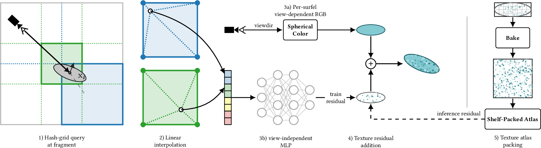
Our method separates scene appearance into a view-independent high-frequency texture residual per-fragment and a per-primitive view-dependent color. During training, we represent the geometry with 2D Beta surfels, and model the texture residual with a spatial multi-resolution hash-grid and a world-space multilayer perceptron (MLP) decoder.
For inference, we sample the hash-grid across the surface of each primitive and bake the output into a compressed RGB texture atlas. This enables fast, per-fragment queries during rendering.
3.1 Differentiable Surfel Splatting↩︎
3DGS [3] maps volumetric ellipsoids to the 2D image plane using EWA splatting [24]. 2DGS [15] flattens these volumetric ellipsoids into oriented planar disks called surfels. We build upon this differentiable 2D surfel representation to model scene geometry accurately while maintaining rendering performance.
Each surfel \(i\) is parameterized by a position \(\mu_i\), rotation \(q_i\), two-dimensional scale \(s_i\), and opacity \(o_i\). The color \(C\) of a pixel is computed by alpha-blending a depth-sorted sequence of N surfels overlapping that screen coordinate. For a given kernel \(G\), the contribution of the \(i-th\) surfel is determined by its opacity \(\alpha_i\) and its spatial influence \(G(x)\), yielding the composition formula: \[C = \sum_{i=1}^{N} c_i(x) \sigma_i \prod_{j=1}^{i-1} (1 - \sigma_j),\] where \(\sigma_i = \alpha_i G(x)\) is the effective transparency at the point \(x\). The color \(c_i(x)\) can be a constant per-surfel value or vary across the position \(x\) for textured surfels. Since the formulation is fully differentiable, it can be optimized against reference images to obtain the 3D model representation.
3.2 Deformable Beta Kernels↩︎
Deformable Beta kernels [9] replace the standard Gaussian kernel with a Beta function using a learnable parameter \(b\) to morph between a Gaussian distribution and an opaque, flat disk. We replace the Gaussian kernel used in 2DGS with this Beta kernel: \[\mathcal{B}(x;b) = (1-x)^{\beta(b)},\quad \beta(b)=4\sigma(b),\quad x \in [0,1], b \in \mathbb{R}, \label{eq:beta-kernel}\tag{1}\] where \(\sigma(\cdot)\) is the sigmoid function and \(x\) is the normalized radial distance from the kernel center. This allows surfels to act as soft elements for large \(b\) values or flat, hard-edged disks for small \(b\) values, reducing overdraw and increasing rendering speed. We restrict the parameter range to keep the kernels between flat uniform distributions and soft Gaussians.
4 Spatial Texture-Atlas Splatting↩︎
We decompose the appearance of each surfel into two learnable components: a per-primitive view-dependent color \(f_{SV}(\mathbf{d})\), and a global view-independent residual \(\boldsymbol{\rho}(\mathbf{x}) = f_\phi(E_\theta(\mathbf{x}))\) produced by a multiresolution hash grid \(E_\theta\) and an MLP decoder \(f_\phi\). A fixed scalar offset \(b_{SV} = 0.5\) inside the inner activation shifts the view-dependent term away from zero, providing a neutral gray baseline on which the residual can build even before \(f_{SV}\) is trained. The total fragment color is evaluated as
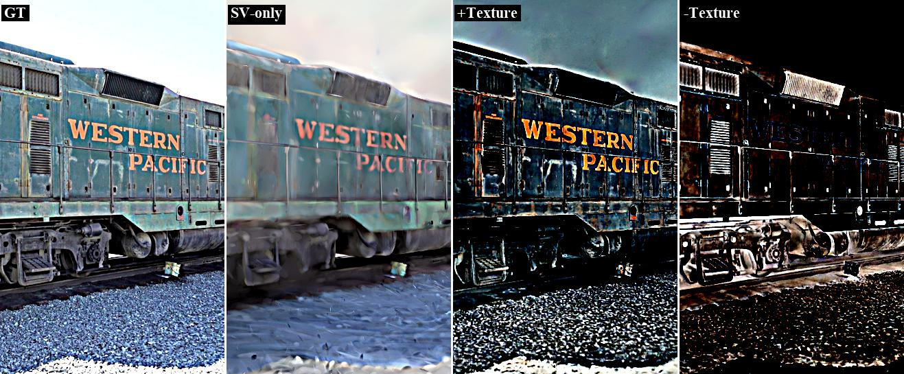
\[\mathbf{c}(\mathbf{x}, \mathbf{d}) = \mathrm{ReLU}\Big( \mathrm{ReLU}\big( f_{SV}(\mathbf{d}) + b_{SV} \big) + f_\phi\!\big(E_\theta(\mathbf{x})\big) \Big). \label{eq:color}\tag{2}\] Since the color texture produces spatially varying outputs for each fragment location \(\mathbf{x}\), low-frequency details and view-dependent reflections are pushed into the per-surfel attributes, while high-frequency, view-independent details are absorbed by the texture, as demonstrated in Fig. 2.
4.1 View-independent Surfel Texture↩︎
The texture mapped to a surfel contributes a color residual that is added to the surfel’s base and view-dependent color. In the training pass, we represent this color residual with a multiresolution hash grid \(E_\theta\) with a fixed-size feature table and a compact view-independent MLP decoder \(f_\phi\). At each fragment location \(\mathbf{x}\), we trilinearly interpolate features from each level of the hash grid, concatenate them, and pass them through the view-independent MLP. These residual values are unbounded, allowing negative and positive offsets. This increases representational capacity and reduces the burden on the surfels to fit base color variations, directly encouraging a sparser primitive count. The hash grid uses four levels with a \(4\)D feature per level and log\(_2\) resolutions ranging from \(8\) to \(11\), and the decoder \(f_\phi\) is an MLP with two hidden layers of width \(16\).
4.2 Texture Baking↩︎
Evaluating the spatial hash grid and MLP during rendering introduces a computational bottleneck. Therefore, after training the view-independent hash grid output is evaluated across each surfel and baked into a global RGB texture atlas for fast inference.
To capture the spatial frequency of the underlying hash grid without wasting memory, we assign an anisotropic UV-grid resolution \(\mathbf{r}_g = (r_x, r_y)\) to each surfel. The residual \(\boldsymbol{\rho}(\mathbf{x}_g)\) is band-limited by the finest hash voxel of \(E_\theta\). We use this limit to match the Nyquist rate of the hash grid along each tangent axis. For an axis \(a \in \{u, v\}\), the resolution is computed as: \[r_{g,a} = \mathrm{clamp}\left(2^{\lceil \log_2(4 e s_{g,a}/\delta) \rceil}, r_{\min}, r_{\max}\right), \label{eq:nyquist}\tag{3}\] where \(s_{g,a}\) is the surfel scale on tangent axis \(a\), \(e=4\sigma\) is the surfel UV extent, and \(\delta\) is the finest hash voxel size. The factor of \(4\) inside the logarithm combines the \(2e\) UV span with the multiplier required for Nyquist sampling. We bound the resolution between \(r_{\min}=4\) and \(r_{\max}=64\). Allowing anisotropic dimensions saves approximately 30% of the atlas area on long, thin surfels. We optionally cap \(r_{g,a}\) by each surfel’s maximum projected pixel extent across training views to avoid over-allocating memory for physically large but distant primitives.
Once the resolutions are determined, the per-surfel grids are stored in an atlas of dimensions \(W \times H\) using a Shelf-First-Fit-Decreasing algorithm. Surfels are sorted descending by \(r_y\), then \(r_x\), and placed into the first available shelf. We fix \(W=4096\) and grow \(H\) greedily, rounding to a
multiple of 64 and automatically increase \(W\) if \(H\) approaches the 65,536-row cudaArray limit.
At the center of each texel, the hash grid and MLP are evaluated. For a texel \((i,j)\) assigned to surfel \(g\), local coordinates are computed using the texel-center convention: \[u = \frac{i + 0.5}{r_x} 2e - e, \quad v = \frac{j + 0.5}{r_y} 2e - e.\] This mapping prevents boundary seams by aligning the baked evaluation with the hardware bilinear sampler. The local coordinates are lifted to world space via the surfel tangent frame \(\mathbf{R}\): \[\mathbf{x} = \mathbf{p}_g + u s_{g,u} \mathbf{R}_{:,0} + v s_{g,v} \mathbf{R}_{:,1}.\] The evaluated RGB vector \(\boldsymbol{\rho}(\mathbf{x})\) is finally written to the atlas using a fused kernel that allocates one warp per texel row.
4.2.0.1 Quantization
Instead of storing a dense FP16 RGB atlas, we apply Block Compression (BC7) to reduce the memory footprint. We compute a scalar range \([\mu - 6\sigma, \mu + 6\sigma]\) via bootstrap sampling and uniformly quantize the atlas with a single global \((\mathrm{offset}, \mathrm{scale})\) pair, written to the bake metadata and applied as a multiply-add per read operation by the rasterizer at inference. The data is padded to RGBA to match the \(4 \times 4\) block layout of BC7. This format stores each block in 16 bytes, reducing the memory requirement to 1 byte per texel. As indicated by Table 1, no perceivable quality loss is introduced by quantization, yet a significant memory reduction is achieved.
| Format | Bytes / texel | Mean atlas size | \(\Delta\)PSNR vs.neural |
|---|---|---|---|
| FP16 RGB (ref.) | 6 | \(\sim\)3.8 GB | — |
| uint8 RGBA | 4 | \(\sim\)2.6 GB | \(\pm\)0.01 dB |
| BC7 RGBA (ours) | 1 | \(\sim\)638 MB | \(\pm\)0.01 dB |
4.3 View-dependent Surfel Color↩︎
To capture view-dependent effects, each primitive utilizes a soft spherical Voronoi representation [19]. This representation partitions the sphere among a set of generator points called sites. Instead of using hard Voronoi cells with sharp boundaries, it defines smooth, differentiable transitions between regions with a continuous weighting function—often obtained via a softmax, radial basis functions, or differentiable distance weighting—so that every surface point has fractional membership in multiple generators. The learnable regions with smooth boundaries provide an explicit and stable parameterization for reflections.
Given a viewing direction \(\mathbf{d}\), the view-dependent color proportion is evaluated as a weighted combination of per-site values: \[f_{SV}(\mathbf{d}) = \sum_{k=1}^{K} w_k(\mathbf{d})\, c_k, \quad w_k(\mathbf{d}) = \frac{\exp(\tau_k\, s_k \cdot \mathbf{d})}{\sum_{k'=1}^{K} \exp(\tau_{k'}\, s_{k'} \cdot \mathbf{d})}.\] Here, \(K\) directional sites \(s_k\) on the unit sphere store learnable color values \(c_k\). The temperature parameters \(\tau_k\) control the angular sharpness of the partition, allowing the model to fit both broad diffuse shifts and sharp specular highlights for each geometric element. The mixture is offset by the fixed constant \(b_{SV}=0.5\) and gated by the inner \(\mathrm{ReLU}\) of Eq. 2 .
4.4 Rendering↩︎
During inference we replace the neural renderer used during training to generate the hash grid with a forward-only 2D splatting rasterizer. For each fragment within a surfel’s footprint, the hardware texture unit samples the BC7 block at the fragment’s UV with bilinear filtering. The dequantized residual \(\hat{\boldsymbol{\rho}}\) is added to the per-primitive view-dependent feature inside the outer \(\mathrm{ReLU}\) of Eq. 2 , before \(\alpha\)-compositing.
5 Optimization↩︎
The typical ADC optimization of 3DGS already converges to a comparatively low primitive count with our hybrid texture-based representation. To further enhance sparsity, we adopt the multi-view error-based optimization of FastGS [6]. An even more aggressive primitive reduction is achieved by incorporating a falloff regularizer on the Beta kernels. Finally, we add a hybrid training strategy to mitigate the training-time bottlenecks of back-propagating into a multi-resolution hash-grid.
5.1 Multi-view Error Optimization↩︎
Standard ADC relies on positional gradients and opacity, which can produce redundant primitives. We replace this with the multi-view consistent densification and pruning strategies from FastGS. It computes an importance score \(s_d^i\) for each primitive \(i\) based on its contribution to the multi-view reconstruction quality. The average number of high-error pixels within the primitive’s two-dimensional footprint \(\Omega_i\) across a sampled set of \(K\) training views is counted as \[s_d^i = \frac{1}{K} \sum_{j=1}^K \sum_{p \in \Omega_i} \mathbb{I}\big(\mathcal{M}^j_{\text{mask}}(p) = 1\big),\] where \(\mathcal{M}^j_{\text{mask}}\) is a binary mask indicating pixels with high photometric error in view \(j\). We use this score to strictly gate densification and pruning. Surfels are densified only if their score exceeds a set threshold, and they are pruned if they provide a negligible contribution to the overall photometric accuracy.

5.2 Falloff Reduction↩︎
While the multi-view error optimization already prunes redundant primitives, each surviving Beta surfel can still spread photometric influence well beyond its geometric core through the soft tail of its kernel. We add a regularizer that gradually tightens this tail by pushing the per-primitive Beta parameter \(\beta_i\) toward smaller, flatter values. To prevent the regularizer from disrupting the early training of soft Gaussian-like kernels, we gate it by the local photometric error: the term self-activates only where the reconstruction is already accurate, so flexible regions stay flexible while already-converged regions are pulled toward hard-edged disks.
| Tanks and Temples | Mip-NeRF 360 | |||||||||
| Method | PSNR\(\uparrow\) | SSIM\(\uparrow\) | LPIPS\(\downarrow\) | Points\(\downarrow\) | FPS\(\uparrow\) | PSNR\(\uparrow\) | SSIM\(\uparrow\) | LPIPS\(\downarrow\) | Points\(\downarrow\) | FPS\(\uparrow\) |
| 3DGS | 23.80 | 0.169 | 1.5M | 154 | 27.21 | 0.214 | 2.7M | 134 | ||
| 2DGS | 23.15 | 0.831 | 0.212 | 0.8M | 122 | 27.04 | 0.252 | 2.0M | 64 | |
| Beta-Splatting (DBS) | 2.0M | 150 | 3.1M | 123 | ||||||
| NeST-Splatting | 23.02 | 0.824 | 0.181 | 0.5M | 30 | 26.68 | 0.795 | 1.0M | 23 | |
| Hybrid Latents | 22.81 | 0.826 | 0.187 | 50 | 26.85 | 0.794 | 0.218 | 36 | ||
| BBSplat | 23.83 | 0.4M | 66 | 26.98 | 0.783 | 0.231 | 0.4M | 25 | ||
| Nexels | 23.55 | 0.841 | 0.4M | 70 | 0.802 | 0.4M | 50 | |||
| FastGS* | 0.839 | 0.210 | 0.797 | 0.261 | 0.40M | |||||
| Ours* | 0.852 | 0.157 | 0.15M | 27.18 | 0.783 | 0.244 | ||||
| Ours (falloff)* | 23.86 | 0.844 | 0.164 | 26.75 | 0.770 | 0.253 | ||||
Given the rendered colour \(\mathbf{C}(p)\) and the ground-truth \(\hat{\mathbf{C}}(p)\) at pixel \(p\), we define an adaptive weight \[\omega(p) = \exp\!\big(-\gamma\, \|\mathbf{C}(p) - \hat{\mathbf{C}}(p)\|_1\big),\] following the HiNeuS error-weighting scheme [25], where \(\gamma\) controls how sharply the weight decays with photometric error. \(\omega(p) \to 0\) on poorly reconstructed pixels and \(\omega(p) \to 1\) where the surfels already fit the ground truth. For each pixel we form an alpha-blended Beta value \(\bar{\beta}(p) = \sum_{i \in \mathcal{N}_p} w_i(p)\, \beta_i\) from the standard \(\alpha\)-blending weights \(w_i(p)\) of the overlapping surfels; the falloff loss is the error-weighted mean across all pixels \(P\): \[\mathcal{L}_{\beta} = \frac{1}{|P|} \sum_{p \in P} \omega(p)\, \bar{\beta}(p).\] This term is added to the photometric objective with weight \(\lambda\), i.e. \(\mathcal{L} = \mathcal{L}_{\text{photo}} + \lambda\,\mathcal{L}_{\beta}\), so that \(\lambda\) sets the overall strength of the falloff reduction.
Because \(\omega\) scales with reconstruction quality, \(\mathcal{L}_\beta\) exerts negligible pressure during the volatile early-training stage, when the photometric loss dominates and \(\omega \approx 0\) across most pixels, and ramps up automatically as the reconstruction converges and \(\omega\) saturates. This avoids any hand-tuned warm-up schedule. Once active, the loss pulls the kernel of each accurate surfel from a soft Gaussian-like tail toward a hard-edged uniform disk, bounding its spatial influence to its geometric extent. As a side benefit, the tightened kernels also reduce fragment overdraw during rasterization, which we exploit at inference time.
5.3 Training Time↩︎
Because the falloff regularizer self-activates only after the photometric reconstruction converges, the rasterizer processes a high volume of fragments during the early training stages. Backpropagating through a multi-resolution hash grid and MLP at each fragment creates a heavy computational bottleneck during this period. We mitigate this overhead by implementing a periodic freezing schedule. After 5000 training iterations, we freeze the MLP and hash grid for nine out of every ten iterations. The spatial texture representation converges rapidly during the early stages of optimization. Freezing these parameters allows the geometric surfels to adjust their positions and fit the stable texture output at a much lower computational cost. We average 45 minutes on training Mip-NeRF 360 scenes.
6 Experiments↩︎
We evaluate our method on all scenes from the Mip-NeRF 360 [26] dataset, along with two scenes from the Tanks and Temples [27] dataset. The comparison is against standard methods using only per-primitive appearance attributes, baselines using per-primitive textures, and FastGS as the sparsification optimization we used. We report PSNR, SSIM, LPIPS, primitive counts (N), and framerate(FPS). We benchmark all timings on an NVIDIA RTX 4090.
6.1 Novel View Synthesis↩︎
We evaluate the photometric quality and representational efficiency of our reconstructions using the standard 3D Gaussian Splatting evaluation pipeline. For the Mip-NeRF 360 dataset, we evaluate on the downsampled images as specified by the dataset guidelines.
Table 2 reports the quantitative comparison. Our method provides a high quality-to-point ratio compared to non-textured methods. The texture residual specifically improves the LPIPS metric by capturing high-frequency details that coarse geometric primitives miss. Compared to existing methods using per-primitive textures, we achieve similar sparsity and quality, but our baked representation enables significantly higher inference speed.
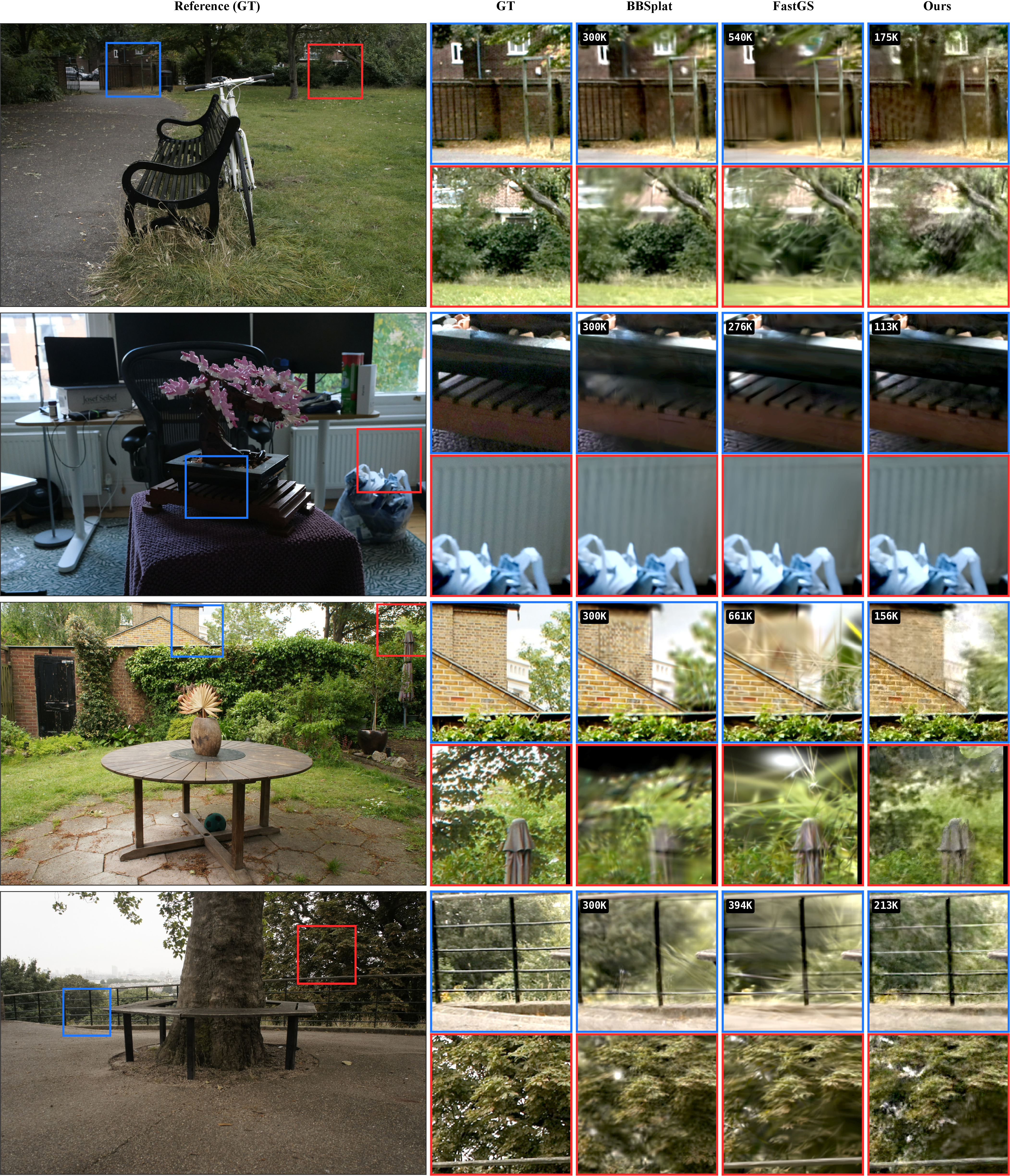
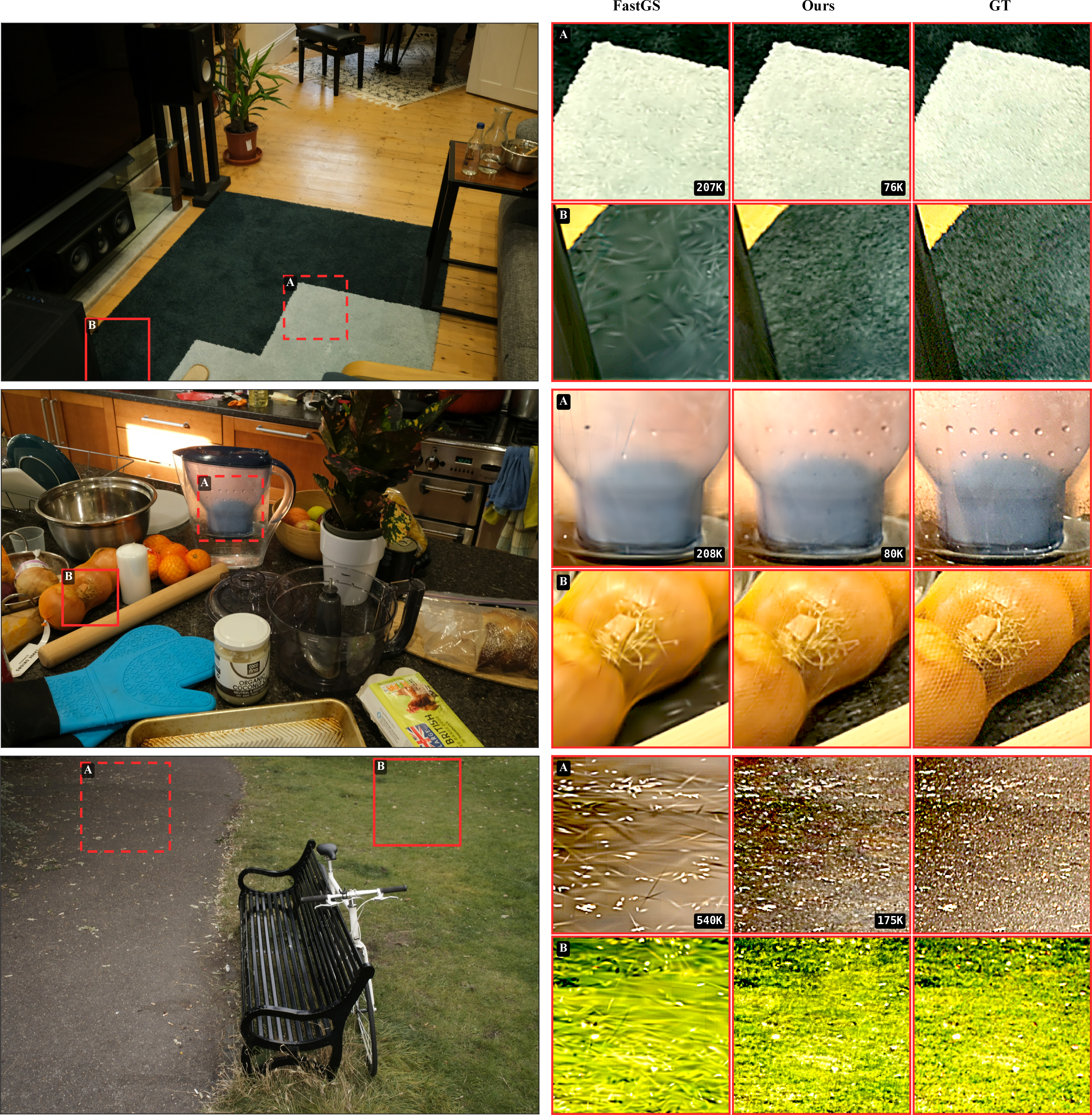
Our method reduces primitive count by roughly 2× relative to FastGS at the cost of slightly lower fidelity in PSNR and slower rendering due to texture coordinate computation overhead. Nevertheless, despite its higher primitive count, FastGS frequently fails to reconstruct textures accurately on both foreground and background objects, as shown in the teaser and Figs. 5 and 4.
6.2 Ablation: Falloff Reduction↩︎
We evaluate the impact of our falloff regularization on the Beta surfels. We compare our unregularized method against two values of the falloff penalty. As a direct consequence of the regularizer, the soft tails of the Beta kernels tighten and fragment overdraw drops; Figure 3 shows the resulting per-pixel intersection count as the falloff weight \(\lambda\) increases, and Table 3 reports the corresponding quality/speed trade-off.
Forcing the Beta kernels to adopt flatter profiles directly reduces the spatial volume of each primitive. This structural change strictly bounds the alpha-blending footprint, which in turn lowers fragment overdraw during rasterization. We make the regularization loss-informed as more Gaussian-like kernels are better for convergence, so the regularizer activates only after the model has trained a little.
| Variant | \(N\) | PSNR\(\uparrow\) | SSIM\(\uparrow\) | LPIPS\(\downarrow\) | FPS\(\uparrow\) |
|---|---|---|---|---|---|
| None (\(\lambda=0\)) | 259,561 | 317 | |||
| \(\lambda=0.001,\, \gamma=25\) | 227,590 | 24.04 | 0.687 | 0.284 | 448 |
| \(\lambda=0.005,\, \gamma=25\) (default) | 23.84 | 0.668 | 0.301 |
6.3 Ablation: Per-primitive Features↩︎
We assess the effect of different view-dependent feature representations on the final primitive count. We replace the standard spherical harmonics with spherical Gaussians, spherical Betas, and spherical Voronoi partitions, as reported in Table 4.
Improving the representational capacity of the per-primitive view-dependent features allows the optimization to fit the scene at a higher-quality with fewer total primitives. Because the hash grid handles the high-frequency spatial texture, the choice of spherical feature primarily affects the sparsity of the geometric base rather than the final LPIPS score.
| Variant | \(N\) | PSNR\(\uparrow\) | Params\(\downarrow\) | FPS\(\uparrow\) |
|---|---|---|---|---|
| SH (deg 3) | 117,082 | 30.88 | 6.91M | 401.5 |
| SV (K=7 sites) (ours) | 112,748 | 6.7M | 576.4 | |
| SB (K=2 lobes) | 31.09 |
7 Limitations and Future Work↩︎
While our periodic hashMLP training strategy accelerates training, significant room remains for convergence analysis and performance optimization. The per-fragment hash-grid forward and backward passes—particularly under high overdraw—become a bottleneck that must be minimized to achieve competitive training times.
The compressed texture atlas still demands substantial memory. In future work, we will explore generating a smaller atlas by leveraging the trained hash grid positional encoding, for instance via a learned mapping to a fixed-size atlas. Furthermore, we will investigate a more efficient way to compute texture coordinates during inference, to further speed up our approach.
Finally, an explicit overdraw reduction loss informed by the per-pixel loss would be a useful direction to further optimize this method.
8 Conclusion↩︎
We introduce a texture-based method for novel view synthesis using 2D surfel splatting. During training, a neural hash grid captures view-independent appearance, which is then baked into a 2D color texture atlas for inference. Extensive experiments show that our approach achieves high inference speed and high-quality reconstruction with a low number of surfels. We demonstrate a superior quality-to-primitive ratio and rendering performance on par with the fastest existing methods, but with significantly higher fidelity.
9 Rasterization Optimizations↩︎
We incorporate architectural improvements from FastGS [6] to maximize rendering speed. We use SnugBox, a tight screen-space bounding box derived directly from the conic equation, which provides numerical stability under edge-on tilts. We also implement AccuTile, an analytic per-row ellipse intersection during the duplicate-keys phase that emits keys only for tiles the ellipse strictly overlaps.
10 Rendering Performance on Consumer Devices↩︎
To further evaluate rendering performance under strict hardware constraints, we also measure novel view synthesis on an Apple MacBook Pro M3 and a Samsung Galaxy S24 Ultra smartphone (see Tab. 5).
| Scene | Res. | \(N\) | RTX 4090 | MBP M3 (18GB) | S24 Ultra |
|---|---|---|---|---|---|
| counter | 1558\(\times\)1038 | 80,135 | 804.0 | 178.2 | 91.4 |
| garden | 1297\(\times\)840 | 156,216 | 951.8 | 254.3 | 117.2 |
Exploiting texture mapping hardware and a minimal set of surfels allows our pipeline to operate at higher framerates than alternative approaches using textures or hash grids, at high rendering quality.
11 Videos and Demos↩︎
We provide decomposition videos of our method on the bicycle and garden scenes from Mip-NeRF 360 and the truck scene from Tanks and Temples. An interactive visualizer, demos, and videos are available on our project page: https://nilkel.github.io/bitymi/.
12 Per-scene results↩︎
| w/ falloff | w/o falloff | |||||||||
| Scene | PSNR | SSIM | LPIPS | \(N\) | FPS | PSNR | SSIM | LPIPS | \(N\) | FPS |
| Pre-baking (neural renderer) | ||||||||||
| bicycle | 23.87 | 0.678 | 0.321 | 174,573 | 97.3 | 24.23 | 0.703 | 0.294 | 259,561 | 61.3 |
| bonsai | 32.11 | 0.930 | 0.222 | 112,748 | 93.5 | 33.00 | 0.941 | 0.215 | 170,137 | 62.4 |
| counter | 29.00 | 0.889 | 0.251 | 80,248 | 93.0 | 29.45 | 0.901 | 0.237 | 121,681 | 65.0 |
| flowers | 20.39 | 0.529 | 0.373 | 213,015 | 83.0 | 20.50 | 0.545 | 0.365 | 300,071 | 52.9 |
| garden | 26.60 | 0.824 | 0.177 | 156,358 | 103.1 | 26.97 | 0.839 | 0.157 | 242,490 | 66.4 |
| kitchen | 30.65 | 0.906 | 0.168 | 147,553 | 76.3 | 31.62 | 0.920 | 0.154 | 237,707 | 52.0 |
| room | 30.31 | 0.904 | 0.282 | 75,598 | 112.7 | 31.00 | 0.913 | 0.269 | 118,038 | 78.0 |
| stump | 25.59 | 0.715 | 0.313 | 102,286 | 107.9 | 25.85 | 0.733 | 0.294 | 151,131 | 69.5 |
| treehill | 22.28 | 0.589 | 0.376 | 212,583 | 76.8 | 22.30 | 0.600 | 0.367 | 317,360 | 45.7 |
| mip-360 mean | 26.76 | 0.774 | 0.276 | 141,662 | 93.7 | 27.21 | 0.788 | 0.262 | 235,356 | 61.5 |
| train | 22.35 | 0.811 | 0.234 | 121,010 | 124.8 | 22.58 | 0.820 | 0.226 | 159,072 | 99.1 |
| truck | 25.37 | 0.877 | 0.154 | 102,085 | 127.8 | 25.70 | 0.884 | 0.145 | 144,649 | 94.4 |
| T&T mean | 23.86 | 0.844 | 0.194 | 111,548 | 126.3 | 24.14 | 0.852 | 0.186 | 151,861 | 96.8 |
| Post-baking (BC7 atlas) | ||||||||||
| bicycle | 23.83 | 0.666 | 0.301 | 173,755 | 621.9 | 24.13 | 0.688 | 0.282 | 259,334 | 280.9 |
| bonsai | 31.91 | 0.929 | 0.206 | 112,481 | 483.4 | 32.80 | 0.939 | 0.205 | 170,063 | 224.9 |
| counter | 28.96 | 0.887 | 0.221 | 80,135 | 804.0 | 29.40 | 0.899 | 0.214 | 121,670 | 438.8 |
| flowers | 20.56 | 0.534 | 0.352 | 212,272 | 460.1 | 20.68 | 0.548 | 0.346 | 299,906 | 205.2 |
| garden | 26.65 | 0.813 | 0.173 | 156,216 | 951.8 | 26.98 | 0.823 | 0.163 | 242,462 | 427.8 |
| kitchen | 30.59 | 0.904 | 0.156 | 147,442 | 609.0 | 31.52 | 0.917 | 0.144 | 237,683 | 357.1 |
| room | 30.36 | 0.902 | 0.240 | 75,207 | 992.2 | 31.03 | 0.910 | 0.235 | 117,936 | 482.8 |
| stump | 25.54 | 0.716 | 0.276 | 102,131 | 585.0 | 25.76 | 0.730 | 0.264 | 151,076 | 257.4 |
| treehill | 22.33 | 0.583 | 0.349 | 211,700 | 470.9 | 22.36 | 0.594 | 0.346 | 317,142 | 197.6 |
| mip-360 mean | 26.75 | 0.770 | 0.253 | 141,260 | 664.3 | 27.18 | 0.783 | 0.244 | 213,030 | 319.2 |
| train | 22.35 | 0.804 | 0.215 | 120,097 | 1038.7 | 22.57 | 0.811 | 0.211 | 158,858 | 659.4 |
| truck | 25.44 | 0.874 | 0.153 | 101,636 | 1149.9 | 25.75 | 0.880 | 0.152 | 144,553 | 637.6 |
| T&T mean | 23.89 | 0.839 | 0.184 | 110,867 | 1094.3 | 24.16 | 0.846 | 0.181 | 151,706 | 648.5 |