Traffic-Aware Randomized Smoothing for LLM-Based Network Intrusion Detection
July 15, 2026
Abstract
Large language model (LLM)-based intrusion detection systems (IDS) are increasingly studied for security monitoring, yet their robustness against feasible traffic manipulation remains largely empirical. We present Traffic-Aware Randomized Smoothing (TA-RS), a classifier-agnostic certified defense that injects Gaussian noise exclusively into the directly controllable (DC) subspace—features a remote attacker can modify—during both fine-tuning and certification, aligning the smoothing distribution with the attacker-controllable subspace. We identify a critical prerequisite: applying standard randomized smoothing to clean-trained LLM-IDS yields weak certified accuracy in three of four (model, dataset) pairs tested (14–33%, at or below random) and only 57% in the fourth (43 pp below the noise-augmented result); noise-augmented fine-tuning recovers to 68–100% on two of three benchmark datasets (at \(\sigma{=}0.25\)). At the L\(_\infty\)-equivalent threshold \(R_\infty{=}\varepsilon\sqrt{|\mathcal{F}_{\mathrm{DC}}|}\) (\(\varepsilon{=}0.05\)), TA-RS achieves 55–100% certified accuracy on CIC-IDS-2018 and HIKARI-2021, with median certified radii (\(\tilde{R}{\approx}0.45\)–\(0.96\)) exceeding \(R_\infty\) by \(1.8\)–\(5{\times}\) (across \(\sigma{=}0.25\)–\(1.00\)). Against a fairly trained iso-trained RS baseline the residual advantage is dataset-dependent (4–19 pp on CIC-IDS-2018). The larger gap—up to 72 pp against an isotropic RS baseline that shares the DC-noise-augmented training recipe—primarily reflects the training–certification mismatch rather than DC alignment alone: isotropic test-time noise perturbs uncontrollable features the attacker cannot exploit, triggering abstention rates up to 68%. RT-IoT2022 probes the limits of the method: it fails under the default fine-tuning recipe but recovers to 76%/69% certified accuracy (LLaMA3-8B/Qwen3-8B) when noise augmentation is increased. The framework provides a principled basis for certified defenses in traffic-domain settings beyond the configurations evaluated.
DC/IC/UC taxonomy identifies which traffic features are attacker-controllable.
Noise-augmented fine-tuning is prerequisite: clean LLMs yield near-random CA.
TA-RS eliminates abstention on non-controllable features (68%\(\to\)8% on CIC).
Anisotropic RS confirms DC-only smoothing is principled (\(\leq\)2 pp difference).
Certified accuracy 55–100% on CIC/HIKARI at L\(_\infty\) budget \(\varepsilon{=}0.05\).
certified robustness, randomized smoothing, network intrusion detection, large language models, adversarial machine learning, traffic-aware noise
1 Introduction↩︎
Network intrusion detection systems (IDS) increasingly employ LLM-style models that classify serialized traffic features into attack categories. Before serialization, however, a network adversary can alter packet sizes, flags, or port numbers—features that remain under attacker control regardless of the classification model.
A companion paper [1] formalizes this attack surface by partitioning network-flow features into directly controllable (DC), indirectly controllable (IC), and uncontrollable (UC) sets. Adversarial perturbations confined to the DC subspace already exceed 60% attack success rate against LLM-IDS on multiple modern datasets. The defense problem is therefore sharply scoped: can we certify the classifier against perturbations the attacker can actually produce?
Empirical defenses—adversarial training [2], [3], preprocessing, anomaly filtering—reduce observed attack success but cannot give a worst-case guarantee outside the attacks used during evaluation. Randomized Smoothing (RS) [4] does provide such a guarantee, but applying it directly to LLM-IDS misses two conditions specific to traffic classification.
The first is threat alignment. Standard RS injects isotropic noise into every feature, including UC features the remote attacker cannot set. Certifying those directions inflates the effective perturbation set beyond what is feasible, and the smoothed classifier frequently abstains on irrelevant noise directions.
The second—and in our experience the more important—is model stability. Clean-trained LLM-IDS are not stable under smoothing noise: in our experiments they reach only 14–57% certified accuracy on CIC-IDS-2018 and HIKARI-2021 before any subspace choice is made. Without DC-noise-augmented fine-tuning, even perfect threat alignment cannot produce a useful certificate.
This paper introduces Traffic-Aware Randomized Smoothing (TA-RS) around these two coupled conditions. TA-RS smooths only the DC feature subspace using \(\mathcal{N}(0,\sigma^2\mathbf{I}_{\mathcal{F}_{\mathrm{DC}}})\) and fine-tunes the classifier with traffic-aware noisy copies so that training and certification occur in the same attacker-controllable subspace. The resulting certificate is a DC-subspace L2 certificate; its relationship to the L\(_\infty\) traffic budgets used in the companion attack model is made explicit rather than assumed.
TA-RS is classifier-agnostic in principle: it can wrap any differentiable or black-box classifier. We instantiate it with LLM-based classifiers because text-serialized inputs accept heterogeneous feature schemas without structural modification. Fixed-feature tabular baselines (e.g., NAXGB) can equally be wrapped by TA-RS within a dataset, but require dimension-matched retraining for new datasets. Section 7.6 shows a key limitation: dataset-specific fine-tuning is non-negotiable, and pretraining knowledge does not transfer without traffic-aware tuning.
The experiments test each condition in turn. Noise-augmented fine-tuning raises certified accuracy from weak clean-trained baselines to 68–100% on CIC-IDS-2018 and HIKARI-2021; with noise-stable models, traffic-aware smoothing then outperforms isotropic smoothing by up to 72 pp (4–19 pp residual advantage against iso-trained RS), mainly by eliminating abstention on non-attacker-controllable noise directions. RT-IoT2022 is included to probe the limits: the default recipe fails (CA \(\leq 24\%\)), but increasing \(n_\mathrm{aug}\) to 4 recovers 76%/69% certified accuracy (LLaMA3/Qwen3), confirming that noise-stability—not DC-alignment—is the binding constraint in the hard case.
Contributions. We make four contributions:
Problem formulation: we operationalize the DC/IC/UC controllability taxonomy as the certification subspace for LLM-based IDS. The taxonomy categorizes features by attacker reachability; the dataset-specific DC masks and feature counts required to reproduce this work are defined in full in Section 4 (Table 1). Theorem 2 applies the Cohen et al. [4] certificate to the DC subspace; the contribution is the problem frame, not the certificate formula.
Noise-stability requirement: we demonstrate that clean-trained LLM-IDS often yield weak certificates under RS, while traffic-aware noise-augmented fine-tuning recovers certified accuracy to 68–100% on CIC-IDS-2018 and HIKARI-2021 (Section 6).
Mechanism and boundary: training–certification match—not DC selection per se—is the binding factor. Against a fairly iso-trained baseline the residual TA-RS advantage is 4–19 pp; matched random-subspace RS performs within 2 pp on average. RT-IoT2022 is the failure-boundary case where noise stability, not threat alignment, is the prerequisite (Section 6.7).
Operational L\(_\infty\) coverage: the DC-subspace L2 certificate covers the L\(_\infty\)-equivalent threat threshold (\(R_\infty{=}\varepsilon\sqrt{|\mathcal{F}_{\mathrm{DC}}|}\), \(\varepsilon{=}0.05\)) for 55–100% of CIC/HIKARI samples, with median certified radii \(1.8\)–\(5{\times}\) above \(R_\infty\) (Section 7.2).
2 Related Work↩︎
2.1 Certified Robustness and the Choice of Perturbation Space↩︎
Formal robustness verification for neural networks began with satisfiability-based exact verifiers [5], [6] and was quickly overtaken by relaxation-based methods (CROWN [7], \(\alpha\)-CROWN) capable of scaling to moderate-depth networks. These approaches yield exact or tight certificates but have not scaled to billion-parameter models. For LLM-IDS, scalability is not the only issue: the certificate must also be stated over a perturbation set that matches what a network attacker can change.
Randomized Smoothing [4] offers a complementary approach: by evaluating the base classifier under Gaussian noise and returning the plurality class, one obtains a smoothed classifier certifiable by a Neyman–Pearson argument. Lecuyer et al. [8] introduced an earlier DP-based framework; Cohen et al.tightened the bound and proved its optimality among all noise-based smoothing approaches. Subsequent work extended RS to other threat models (L1, Lp via general smoothing distributions [9]), improved the base classifier with adversarial training of the smoothed model [10], and analyzed failure modes of RS [11]. Derandomized Smoothing [12] achieves certificates against patch attacks by averaging over non-overlapping patches rather than Gaussian noise. Anisotropic randomized smoothing [13] optimizes per-feature noise variances data-drivenly to maximize certified accuracy. TA-RS fixes \(\sigma_{\mathrm{DC}}{=}\sigma\), \(\sigma_{\mathrm{IC/UC}}{=}0\) based on threat-model semantics: noise outside \(\mathcal{F}_{\mathrm{DC}}\) is wasted budget that increases abstention without covering additional attack directions. Neither this nor prior RS work addresses which traffic features should be perturbed when the attacker is bounded to a known feature subspace. TA-RS retains the same certification principle but restricts smoothing support to the DC subspace.
2.2 Feasible Adversarial Perturbations in Network IDS↩︎
The vulnerability of ML-based IDS to adversarial examples was established early [3], [14], [15]. Subsequent work demonstrated practical evasion of deep-learning IDS [16], [17] and proposed empirical countermeasures such as adversarial training [2], ensemble defenses, and input normalization [18]. These defenses are evaluated against specific attacks; they do not give a worst-case certificate over a specified traffic-feature set.
Feature-space constraints are central in network security. Constraint-aware attacks, including the problem-space perspective of Pierazzi et al. [19], demonstrate that semantic feasibility changes the effective perturbation space—a certificate for IDS should therefore be defined over attacker-controllable coordinates, not the full feature vector.
2.3 LLM-Based Security Models and Noise Stability↩︎
LLMs have been applied to log analysis [20], vulnerability description [21], and threat intelligence [22]. For intrusion detection, pre-trained language models have also been adapted to network-traffic classification. These systems serialize structured traffic features into text-like inputs, so small feature perturbations can change the prompt received by the model. The question is therefore not only whether an LLM-IDS is accurate on clean traffic, but whether its predictions remain stable under the feature perturbations used by a certifier.
Randomized smoothing assumes a stable base classifier; without it, the smoothed classifier abstains or collapses to a weak majority. Existing LLM-IDS studies do not establish this condition under traffic-feature noise. Our companion work [1] provides the feasible attack model; this paper asks what training and smoothing distribution are needed to certify an LLM-IDS within it.
3 Preliminaries↩︎
3.1 LLM-IDS Pipeline↩︎
Let \(\mathbf{x} \in \mathbb{R}^d\) denote a normalized network-flow feature vector. An LLM-IDS applies a serialization function \(\text{ser}: \mathbb{R}^d \to \Sigma^*\) (mapping feature values to a natural language prompt) and a fine-tuned LLM \(\text{LM}: \Sigma^* \to \mathcal{Y}\) (mapping prompts to class labels), so \(f(\mathbf{x}) = \text{LM}(\text{ser}(\mathbf{x}))\).
3.2 Attacker Capability Model↩︎
Following [1], we partition the \(d\) features into three disjoint sets:
Directly controllable (DC): \(\mathcal{F}_{\mathrm{DC}}\subset [d]\), features the attacker can set precisely (e.g., destination port, TCP flags, packet sizes, window size). \(|\mathcal{F}_{\mathrm{DC}}|\) ranges from 14 to 27 depending on the dataset (CIC-IDS-2018: 14, HIKARI-2021: 25, RT-IoT2022: 27).
Indirectly controllable (IC): features that emerge from sustained behavioral patterns (e.g., inter-arrival time statistics, flow rate aggregates).
Uncontrollable (UC): features determined by the remote host or network infrastructure (e.g., destination byte counts, server response metrics).
Table 1 lists the DC features for each dataset evaluated in this paper, grounded in network-protocol semantics: these are the forward-direction header and payload fields an attacker sets when crafting or replaying traffic, independent of what the network or remote host does. The IC features (flow-level aggregates, inter-arrival statistics) require sustained behavioral manipulation and are excluded; UC features are fully determined by the remote host or infrastructure.
Timing features illustrate the classification boundary. Forward inter-arrival time (IAT) fields—the delays between packets the attacker sends—are DC for HIKARI-2021 and RT-IoT2022, because the attacker schedules their own outgoing packets
regardless of server behavior. Bidirectional flow-level IAT aggregates (e.g., Flow IAT Mean/Std in CIC-IDS-2018) are IC, because they reflect both attacker-side and server-side packet timing and cannot be set precisely by the attacker
alone.
| Dataset | \(|\DC|\) | DC feature groups |
|---|---|---|
| CIC-IDS-2018 | 14 | Dst port, protocol; fwd pkt/byte counts; |
| TCP flags (FIN/SYN/RST/PSH/ACK, binary); | ||
| fwd header len; init fwd win bytes; fwd data pkts | ||
| HIKARI-2021 | 25 | Orig/resp port; fwd pkt/data counts; |
| fwd header size (tot/min/max); TCP flags (PSH/URG); | ||
| fwd payload stats (min/max/tot/avg/std); | ||
| fwd IAT (min/max/tot/avg/std); | ||
| fwd subflow/bulk bytes & pkts; fwd win sizes | ||
| RT-IoT2022 | 27 | Orig/resp port, proto, service; |
| fwd pkt/data counts; fwd header size (tot/min/max); | ||
| fwd flags (PSH/URG); fwd payload stats; | ||
| fwd IAT stats; fwd subflow/bulk stats; | ||
| fwd init/last window size |
3pt
Remark 1 (Feature independence). The DC-subspace noise model perturbs each DC feature independently. Features with natural statistical dependencies (e.g., fwd_iat_avg and fwd_iat_std) occupy a constrained manifold, so
an adversary restricted to feasible traffic vectors cannot exploit the full L2 ball. The certificate’s soundness is unaffected—independent Gaussian noise subsumes feasible adversarial perturbations, so the stated radius is a valid lower bound—but the
certificate may be conservative relative to a tighter analysis of the feasible manifold.
Let \(\mathbf{I}_{\mathcal{F}_{\mathrm{DC}}} \in \{0,1\}^{d \times d}\) be the diagonal indicator matrix for DC features (\([\mathbf{I}_{\mathcal{F}_{\mathrm{DC}}}]_{ii} = 1\) iff \(i \in \mathcal{F}_{\mathrm{DC}}\), zero otherwise).
3.3 Threat Model↩︎
An adversary observes a flow \(\mathbf{x}\) that \(f\) correctly classifies as malicious and seeks a perturbation \(\boldsymbol{\delta}^*\) with support in \(\mathcal{F}_{\mathrm{DC}}\) such that \(f(\mathbf{x} + \boldsymbol{\delta}^*) \neq f(\mathbf{x})\). The attacker’s budget is parameterized by \(\varepsilon \in \{0.05, 0.15, 0.30\}\) (L\(_\infty\) norm over DC features in normalized space), consistent with [1]. We seek a defense that certifies \(g(\mathbf{x} + \boldsymbol{\delta}^*) = f(\mathbf{x})\) for all \(\boldsymbol{\delta}^*\) with \(\mathrm{supp}(\boldsymbol{\delta}^*) \subseteq \mathcal{F}_{\mathrm{DC}}\) and \(\left\|\boldsymbol{\delta}^*\right\|_2 \leq R\) for a certifiable radius \(R\). Note that the attacker budget is in L\(_\infty\) while the certificate derived in this paper is in L2; the two are related but not equivalent. Remark 3 and Section 7.2 make this gap explicit, and TA-RS should not be interpreted as a full L\(_\infty\) certificate against the companion threat budget.
3.4 Randomized Smoothing (Cohen et al.)↩︎
Definition 1 (Smoothed classifier). Given a base classifier \(f: \mathbb{R}^d \to \mathcal{Y}\) and noise distribution \(\mathcal{N}(0, \sigma^2 \mathbf{M})\) parameterized by positive semidefinite \(\mathbf{M}\), the smoothed classifier is \[g(\mathbf{x}) = \mathop{\mathrm{arg\,max}}_{c \in \mathcal{Y}} \Pr_{\boldsymbol{\delta} \sim \mathcal{N}(0,\sigma^2\mathbf{M})} \!\bigl[f(\mathbf{x} + \boldsymbol{\delta}) = c\bigr]. \label{eq:smooth}\tag{1}\]
Theorem 1 (Cohen et al., 2019). Let \(\mathbf{M} = \mathbf{I}\) (isotropic noise). Suppose \(g(\mathbf{x}) = c_A\) and let \(p_A= \Pr[f(\mathbf{x}+\boldsymbol{\delta}) = c_A]\). If \(p_A> \tfrac{1}{2}\), then \(g(\mathbf{x} + \boldsymbol{\delta}^*) = c_A\) for all \(\left\|\boldsymbol{\delta}^*\right\|_2 \leq \sigma\Phi^{-1}(p_A)\).
4 Traffic-Aware Randomized Smoothing↩︎
TA-RS operationalizes the two conditions introduced above. The smoothing distribution is aligned with the attacker’s feasible feature subspace, and the base LLM is trained to be stable under that same distribution. The first design choice determines what perturbations the certificate covers; the second determines whether the smoothed classifier can make a non-abstaining prediction under those perturbations.
4.1 Traffic-Aware Noise Distribution↩︎
The threat-alignment component is the smoothing distribution. Standard RS uses \(\mathbf{M}=\mathbf{I}\) and perturbs every feature. TA-RS instead perturbs only DC features: \[\boldsymbol{\delta} \sim \mathcal{N}\!\bigl(\mathbf{0},\, \sigma^2 \mathbf{I}_{\mathcal{F}_{\mathrm{DC}}}\bigr), \label{eq:ta95noise}\tag{2}\] where \(\mathbf{I}_{\mathcal{F}_{\mathrm{DC}}}\) is the DC indicator matrix (Section 3.2). This choice does not change the randomized-smoothing principle; it changes the support of the noise so that the smoothed classifier is evaluated in the same feature subspace that the attacker can directly manipulate. The empirical claim tested in Section 6 is that this alignment reduces abstention relative to isotropic smoothing.
Discrete DC features. Some DC features are integer-valued (e.g., packet counts, port numbers). The implementation clips noisy samples to protocol-specified per-feature bounds: \(x_i' = \mathrm{clip}(x_i + \delta_i,\, [\ell_i, u_i])\), where \([\ell_i, u_i]\) is the per-feature normalized range derived from domain-defined limits (e.g.non-negative packet counts, binary flag range \([0,1]\)), not from any statistics of the observed data. Because clip is a deterministic non-expansive map, defining the composed classifier \(h(\mathbf{x}) = f(\mathrm{clip}(\mathbf{x}))\) absorbs this step into the base classifier; Theorem 2 applies to \(h\) exactly, without approximation. The following characterizes what this means for each discrete feature type.
For count-valued DC features (port, packet count, byte count, header length, window size), normalization places each integer step at \(\Delta_i = 1/(\max_i - \min_i)\), which is \(\leq 10^{-4}\) across all evaluated datasets. Since \(\Delta_i \ll \sigma{=}0.25\), the rounding error is negligible and the continuous certificate holds to high accuracy.
For binary flag DC features (TCP flag bits, normalized to \(\{0,1\}\)), rounding constitutes a threshold operation with boundary at \(0.5\). Crucially, the smallest certified radius used in this paper is \(r{=}0.05\) and the largest is \(r{=}0.15\), both strictly below the rounding boundary \(0.5\). An L2-bounded adversary with budget \(R \leq 0.15\) therefore cannot shift any binary flag feature past the rounding threshold deterministically. As a result, the continuous Gaussian certificate at \(r \leq 0.15\) is conservative for binary flag features: the true discrete robustness guarantee is at least as strong as the stated L2 bound, because the adversary’s budget does not suffice to flip any flag with certainty. Section 7.7 discusses the residual discretization gap and a path to a fully rigorous mixed certificate.
For categorical DC features (e.g., proto and service in RT-IoT2022), each category is encoded as a normalized integer label. The composed classifier \(h(\mathbf{x}) =
f(\mathrm{ser}(\mathrm{clip}(\mathbf{x}+\boldsymbol{\delta})))\) absorbs the full preprocessing pipeline—including nearest-integer recovery—into the base classifier; Theorem 2 applies to \(h\) exactly. The normalized step per category \(\Delta_i = 1/(C_i-1)\) is \(0.5\) for proto
(\(C_i{=}3\)) and \({\approx}0.015\) for service (\(C_i{=}66\)), placing both within the conservative regime established for count features.
4.2 Noise-Augmented Fine-Tuning↩︎
The stability component is the training distribution. A smoothed classifier is useful only if the base classifier gives consistent predictions under the same noise used at certification time. This is especially important for serialized LLM-IDS: a small change in a numeric feature can change the prompt tokens and shift the model’s output distribution. Consistent with image-domain RS practice, where Gaussian augmentation improves smoothed accuracy [10], we train the LLM on the same DC-subspace noise used by the certifier.
For each training sample \((\mathbf{x}, y)\), traffic-aware noise-augmented fine-tuning includes one clean copy and \(K{=}2\) noisy copies \((\mathbf{x}+\boldsymbol{\delta}_k,y)\), with \(\boldsymbol{\delta}_k \sim \mathcal{N}(0,\sigma_{\mathrm{train}}^2 \mathbf{I}_{\mathcal{F}_{\mathrm{DC}}})\) as in Eq. 2 and \(\sigma_{\mathrm{train}}=0.25\). The purpose of this module is not to change the certified set; that set is fixed by Eq. 2 and Theorem 2. Its purpose is to make the base LLM stable enough that the smoothed classifier can avoid abstention.
4.3 Certification Procedure↩︎
Given the aligned noise distribution and the noise-augmented base model, certification follows the standard RS two-stage structure. For a test sample \(\mathbf{x}\), TA-Certify first identifies the top class under DC-subspace noise and then estimates a lower confidence bound on the probability of that class. Algorithm 1 describes the procedure.
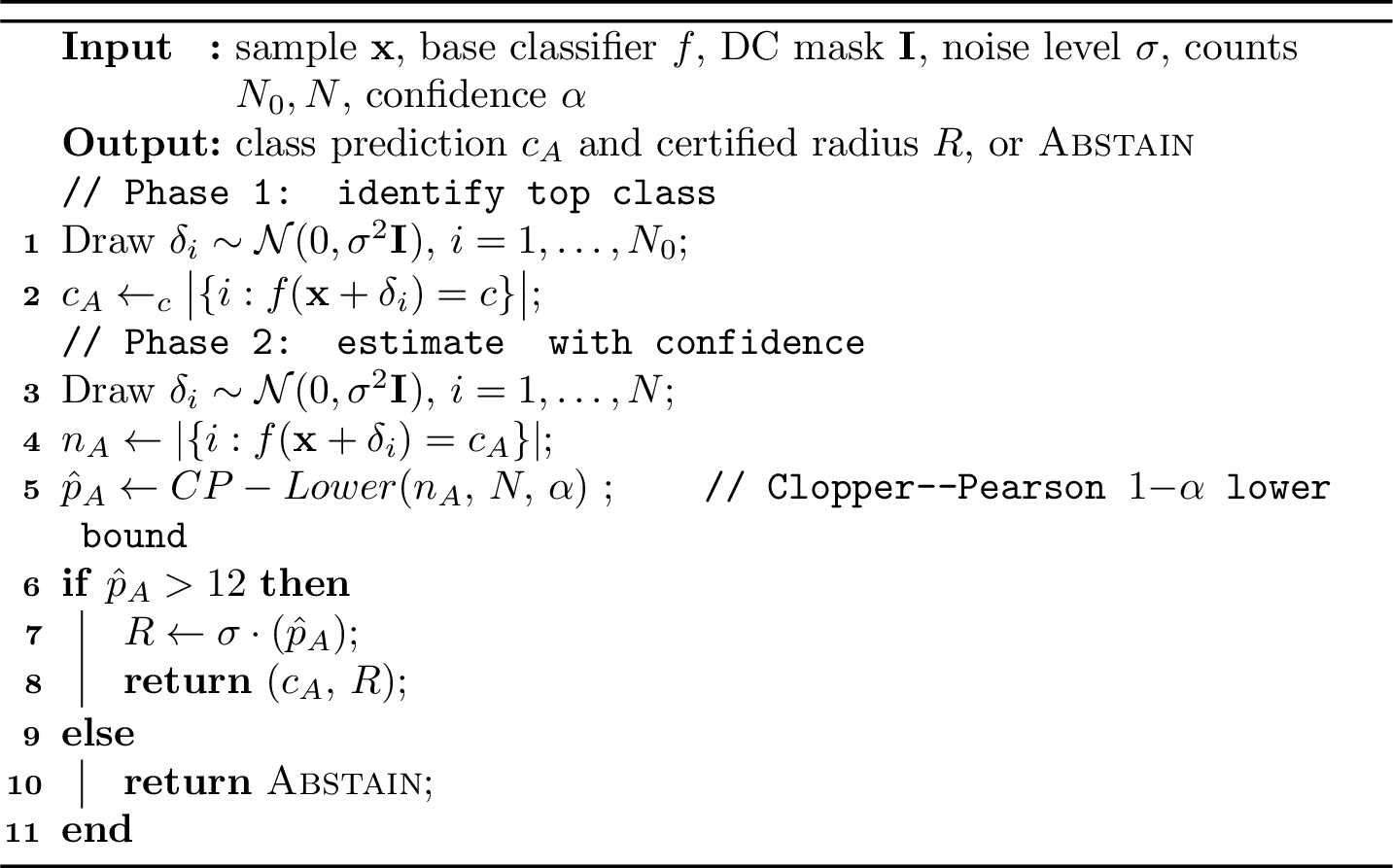
We employ \(N_0 {=} 20\), \(N {=} 200\), \(\alpha {=} 0.001\) throughout. The value \(N{=}200\) is smaller than typical image-domain RS because each certification sample requires LLM inference; the consequence is a conservative Clopper–Pearson lower bound, analyzed in Section 7.
4.4 Certified Accuracy Metric↩︎
The evaluation metric must penalize both instability and wrong predictions. We therefore report certified accuracy at radius \(r\): \[\mathrm{CA}(r) = \frac{1}{|S|} \sum_{\mathbf{x} \in S} \mathbf{1}\bigl[g^{\mathrm{TA}}(\mathbf{x}) = y_{\mathbf{x}} \;\wedge\; R(\mathbf{x}) \geq r\bigr], \label{eq:ca}\tag{3}\] where \(S\) is the evaluation set. Crucially, \(\mathrm{CA}(r)\) penalizes both incorrect predictions and abstentions, so a classifier that predicts a majority class under noise cannot obtain a high score unless it is also correct and certified.
4.5 Formal Guarantee↩︎
The theorem below states what the preceding design certifies. It is a DC-subspace version of the randomized-smoothing guarantee: the support condition on \(\boldsymbol{\delta}^*\) is part of the claim, not a post-hoc interpretation.
Theorem 2 (Traffic-Aware Certified Robustness). Let \(g^{\mathrm{TA}}\) be defined by 1 with \(\mathbf{M} = \mathbf{I}_{\mathcal{F}_{\mathrm{DC}}}\). Suppose \(g^{\mathrm{TA}}(\mathbf{x}) = c_A\) and \(p_A= \Pr_{\boldsymbol{\delta}\sim\mathcal{N}(0,\sigma^2 \mathbf{I}_{\mathcal{F}_{\mathrm{DC}}})}[f(\mathbf{x}+\boldsymbol{\delta})=c_A] > \tfrac{1}{2}\). Then for every \(\boldsymbol{\delta}^*\) satisfying \(\mathrm{supp}(\boldsymbol{\delta}^*) \subseteq \mathcal{F}_{\mathrm{DC}}\) and \(\left\|\boldsymbol{\delta}^*\right\|_2 \leq \sigma\Phi^{-1}(p_A)\), \[g^{\mathrm{TA}}(\mathbf{x} + \boldsymbol{\delta}^*) = c_A.\]
Proof. Since \(\boldsymbol{\delta}\) and \(\boldsymbol{\delta}^*\) both have support in \(\mathcal{F}_{\mathrm{DC}}\), restricting to \(\mathcal{F}_{\mathrm{DC}}\) yields an injection \(\mathbb{R}^{\mathcal{F}_{\mathrm{DC}}} \hookrightarrow \mathbb{R}^d\) that preserves inner products and norms. Within \(\mathcal{F}_{\mathrm{DC}}\), the distribution \(\mathcal{N}(0, \sigma^2 \mathbf{I}_{\mathcal{F}_{\mathrm{DC}}})\) restricted to \(\mathcal{F}_{\mathrm{DC}}\) is \(\mathcal{N}(0, \sigma^2 \mathbf{I}_{|\mathcal{F}_{\mathrm{DC}}|})\). The Neyman–Pearson argument of Cohen et al. [4] applies in \(\mathbb{R}^{|\mathcal{F}_{\mathrm{DC}}|}\) verbatim, yielding the radius \(R = \sigma\Phi^{-1}(p_A)\) within \(\mathcal{F}_{\mathrm{DC}}\). Because \(\mathrm{supp}(\boldsymbol{\delta}^*) \subseteq \mathcal{F}_{\mathrm{DC}}\) by assumption, the certificate transfers to the full feature space. ◻
Remark 2 (Subspace scope). The guarantee is stated over the directly controllable subspace: it certifies perturbations in \(\mathcal{F}_{\mathrm{DC}}\) with \(\left\|\boldsymbol{\delta}^*\right\|_2 \leq R\). Isotropic RS (\(\mathbf{M}=\mathbf{I}\)) produces a certificate of the same form but for the full \(\mathbb{R}^d\) space, certifying against perturbations in UC/IC dimensions that the attacker cannot produce. This broader certificate can be useful if the threat model includes those dimensions, but it is mismatched to the capability-constrained traffic adversary studied here.
Remark 3 (L2 certificate vs.L\(_\infty\) threat budget). The companion threat model [1] bounds adversarial perturbations in L\(_\infty\): \(\left\|\boldsymbol{\delta}^*\right\|_\infty \leq \varepsilon\) over DC features. Our certificate is in L2: it guarantees robustness for \(\left\|\boldsymbol{\delta}^*\right\|_2 \leq R\). These norms are related by \(\left\|\cdot\right\|_\infty \leq \left\|\cdot\right\|_2 \leq \sqrt{|\mathcal{F}_{\mathrm{DC}}|}\,\left\|\cdot\right\|_\infty\), so a certificate at \(R{=}0.05\) (L2) covers L\(_\infty\) perturbations up to \(R/\sqrt{|\mathcal{F}_{\mathrm{DC}}|} \approx 0.010\)–\(0.013\), smaller than \(\varepsilon_{\min} {=}0.05\). Conversely, the L2 norm of an L\(_\infty\) adversarial example with \(\varepsilon{=}0.05\) is at most \(0.05\sqrt{|\mathcal{F}_{\mathrm{DC}}|} \approx 0.19\)–\(0.26\); our certified radii (\(r{=}0.05\) or \(r{=}0.15\)) therefore do not fully cover the companion threat budget. The second conversion (\(R \geq \varepsilon\sqrt{|\mathcal{F}_{\mathrm{DC}}|}\)) is more useful: it identifies the L2 radius at which a certificate directly covers an L\(_\infty\) adversary; Section 7.2 reports what fraction of CIC/HIKARI samples exceed this threshold.
5 Experimental Setup↩︎
The experiments are organized around the two requirements in the central claim. First, the base LLM must make stable predictions under noise restricted to directly controllable traffic features. Second, the certificate should improve because the smoothing distribution matches the attacker’s feasible feature subspace, not because the baseline is weaker or the evaluation radius is easier. The setup therefore keeps the base model, certification budget, sample count, and noise level matched whenever TA-RS is compared with isotropic RS.
5.1 Datasets↩︎
We evaluate these requirements on three modern network-traffic benchmark datasets:
CIC-IDS-2018 [23]: four-class classification (DoS, Normal, Exploitation, CredentialAccess) on 2018 network traces; 25 flow-level features after preprocessing, of which 14 are directly controllable (DC). This is the most label-diverse dataset in our evaluation.
HIKARI-2021: three-class classification (CredentialAccess, Exploitation, Normal) on encrypted traffic features; 82 features after preprocessing, of which 25 are DC. Distinctive per-class feature distributions make this a relatively structured dataset.
RT-IoT2022: five-class classification (CredentialAccess, DoS, Exploitation, Normal, Probe) over IoT traffic with heterogeneous device fingerprints and attack types; 83 features after preprocessing, of which 27 are DC. High within-class feature variability makes this the most challenging dataset for certification.
Table 2 summarises the three datasets. All experiments employ a fixed prompt-aware train/test split to prevent prompt-template leakage between training and evaluation. The StandardScaler normalisation is
fitted exclusively on the training split and applied without refitting to the test split. Feature clipping bounds \([\ell_i, u_i]\) are protocol-derived constants (e.g.packet-count non-negativity, binary flag range \([0,1]\)) and are not estimated from any data split. The certification subset is drawn once from the held-out test split using a fixed random seed (42) and was not used for model selection or hyperparameter tuning.
| Dataset | Classes | Features | DC features | Cert.subset |
|---|---|---|---|---|
| CIC-IDS-2018 | 4 | 25 | 14 | 160 |
| HIKARI-2021 | 3 | 82 | 25 | 120 |
| RT-IoT2022 | 5 | 83 | 27 | 168\(^{\dagger}\) |
| \(^{\dagger}\)One minority class contributes 8 samples (test-set availability). | ||||
5pt
We do not evaluate on NSL-KDD or UNSW-NB15 in this work. NSL-KDD uses one-hot encoding that inflates the raw 48-feature space to 122 dimensions after encoding; our perturbation budget is defined over the raw 48-feature space, so DC-subspace certification is not well-defined in the encoded representation. UNSW-NB15 raises the same issue: the 42-feature DC/IC/UC taxonomy is defined at the raw-feature level, but the data pipeline encodes categorical fields into a 193-dimensional vector, leaving the DC subspace ambiguous. CICIoT2023 [24] is a natural candidate for future evaluation; we defer it because it requires extending the DC/IC/UC taxonomy and re-validating the perturbation budget alignment, which is orthogonal to the certification framework studied here. We discuss dataset scope in Section 7.7.
5.2 Base Classifiers↩︎
We evaluate two 8-billion-parameter LLMs fine-tuned for network traffic classification: Qwen3-8B [25] and LLaMA3-8B [26]. Both models receive serialized feature prompts produced by a dataset-specific template that converts normalized flow features into natural language descriptions. For noise-augmented fine-tuning, we extend the training set with \(K\) traffic-aware noisy copies per sample at \(\sigma{=}0.25\). The default is \(K{=}2\) (\(n_\text{aug}{=}2\)); the effect of increasing to \(K{=}4\) (\(n_\text{aug}{=}4\)) is studied as a sensitivity experiment for RT-IoT2022 (Section 6.6), where greater noise exposure is required to stabilize the base model.
5.3 Baselines↩︎
The baselines separate three claims: whether certification is absent without smoothing, whether noise-augmented LLMs can be certified, and whether restricting smoothing to \(\mathcal{F}_{\mathrm{DC}}\) matters once the model has been trained for noisy inputs. The main comparison (Table 4) uses three configurations:
Undefended: clean-trained LLM-IDS with no smoothing—certified accuracy is zero by definition.
Isotropic RS (noise-aug): the same DC-noise-augmented model wrapped with isotropic Gaussian noise at matching \(\sigma\), certifying in \(\mathbb{R}^d\) rather than \(\mathcal{F}_{\mathrm{DC}}\).
TA-RS (ours): DC-noise-augmented model with traffic-aware Gaussian noise, certifying in \(\mathcal{F}_{\mathrm{DC}}\).
Baseline (2) uses the same fine-tuned model as TA-RS; the only test-time difference is the noise support. This isolates threat alignment from training, but does not preclude the possibility that isotropic RS could benefit from a separately tuned training recipe. Two supplementary controls address this and a second confound:
Isotropic RS (iso-trained): a model fine-tuned with isotropic Gaussian noise augmentation and certified with isotropic RS. This controls for training-recipe asymmetry.
Random-subspace RS: the DC-noise-augmented model certified with noise restricted to a randomly chosen subspace of size \(|\mathcal{F}_{\mathrm{DC}}|\) (seed 99). This controls for the possibility that the TA-RS advantage arises from dimensionality reduction rather than from DC-alignment specifically. The expected overlap between a random subspace of size \(|\mathcal{F}_{\mathrm{DC}}|\) and the true DC set is \(|\mathcal{F}_{\mathrm{DC}}|^2 / d\) per dataset (CIC: \(14^2/25{\approx}7.8\), HIKARI: \(25^2/82{\approx}7.6\), RT-IoT: \(27^2/83{\approx}8.8\) out of \(|\mathcal{F}_{\mathrm{DC}}|\) features), so the random baseline intentionally samples many non-DC features.
Results for baselines (4) and (5) are reported in Section 6.7.
5.4 Certification Parameters and Metrics↩︎
We employ \(N_0{=}20\) samples for class selection, \(N{=}200\) Monte Carlo iterations for probability estimation, and \(\alpha{=}0.001\) (confidence \(1{-}\alpha = 99.9\%\)). These values determine the conservativeness of the certificate and are shared across TA-RS and isotropic RS. Each certification run evaluates 40 samples per class (stratified), yielding 160 test samples per (model, dataset) configuration for CIC-IDS-2018 (4-class), 120 for HIKARI-2021 (3-class), and 168 for RT-IoT2022 (5-class; one minority class contributes 8 samples due to test-set availability). All reported CA values are macro-averaged over classes (not weighted by natural traffic distribution).
We certify at three noise levels \(\sigma \in \{0.25, 0.50, 1.00\}\). The primary metric is \(\mathrm{CA}(r)\) (equation 3 ) at \(r \in \{0.05, 0.10, 0.15\}\) (L2 norm in \(\mathcal{F}_{\mathrm{DC}}\)), because it counts only samples that are both correctly classified and certified. The secondary metrics diagnose why certification succeeds or fails: abstention rate \(\mathrm{AR}\) measures whether the probability lower bound exceeds the decision threshold; smooth accuracy \(\mathrm{SA} = \Pr[g^{\mathrm{TA}}(\mathbf{x}) = y]\) measures whether the smoothed classifier remains correct; and median certified radius \(\tilde{R}\) over non-abstained samples measures the margin of the certificate. For aggregate proportions, we report Wilson 95% confidence intervals when the interval affects interpretation.
5.5 Implementation Notes↩︎
All experiments employ a single NVIDIA RTX PRO 6000 Blackwell (97 GB VRAM) in BF16 precision; per-(model, dataset) certification across all \(\sigma\) values takes 1–2 hours. Both LLMs are fine-tuned with LoRA [27] (\(r{=}16\), \(\alpha{=}32\), dropout 0.05 on q/k/v/o projections), 5 epochs,
effective batch 32, lr \(10^{-4}\) cosine with 5% warmup, seed 42. Noise augmentation appends \(K{=}2\) DC-noisy copies per training sample (\(3\times\)
dataset), generated with \(\mathcal{N}(0,\sigma^2\mathbf{I}_{|\mathcal{F}_{\mathrm{DC}}|})\) at \(\sigma{=}0.25\) clipped to protocol-specified feature bounds. Qwen3-8B uses ChatML format;
LLaMA3-8B uses raw completion; inference is greedy (max_new_tokens=16, batch 64), taking the first valid class token. DC masks are derived from the feature_taxonomy module: 14/25/27 DC features out of 25/82/83 total for
CIC-IDS-2018/HIKARI-2021/RT-IoT2022.
6 Results↩︎
The results follow the same logic as the method. Section 6.1 tests whether an LLM-IDS can be certified without first learning stable predictions under DC noise. Section 6.2 tests whether, given a noise-augmented base model, aligning the smoothing distribution with \(\mathcal{F}_{\mathrm{DC}}\) improves certified accuracy over full-space smoothing. Sections 6.3–6.6 explain the mechanism and the failure case. Section 6.8 checks that the certified lower bound is consistent with empirical transfer-attack robustness, without treating the empirical attack as a substitute for certification.
6.1 Finding 1: Certification Requires Noise-Stable LLM Predictions↩︎
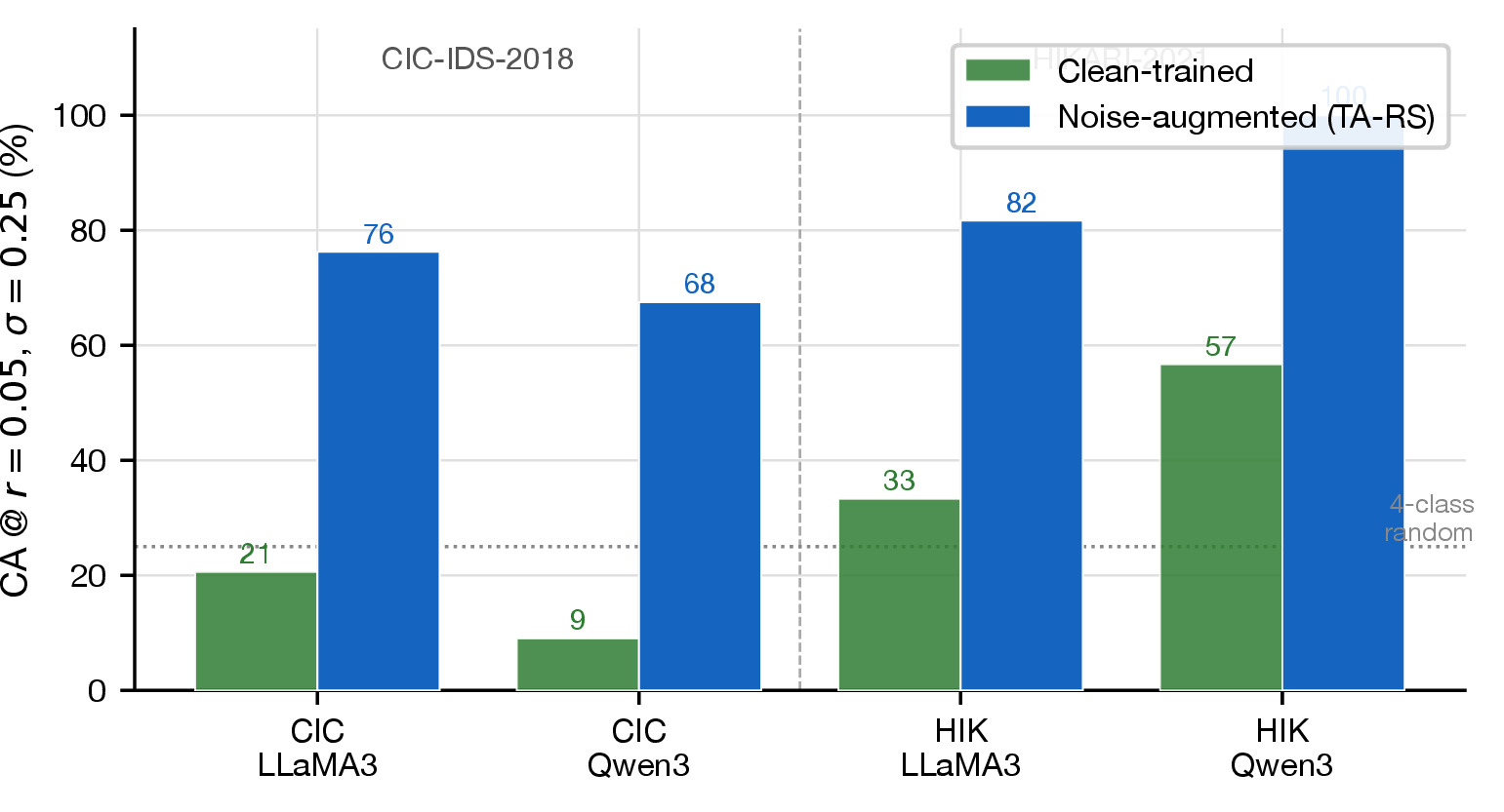
Table 3 asks whether threat-aligned smoothing alone is enough. The answer is no. Clean-trained LLM-IDS models degrade under TA-RS: LLaMA3-8B falls to the random baseline on both datasets (\(20.6\%\) on CIC, \(33.3\%\) on HIKARI), while Qwen3-8B on HIKARI retains moderate certified accuracy (\(57\%\), still 43 pp below the noise-augmented result). On CIC-IDS-2018, both models fall to or below the 4-class random baseline (\(25\%\)). These rows support the first condition in the thesis: the LLM must be stable under the same DC feature noise used for certification.
After noise-augmented fine-tuning, \(\mathrm{CA}(0.05)\) recovers to \(68\)–\(100\%\) on these two datasets (\(+43\)–\(55\) pp). Noise augmentation is not universally sufficient—RT-IoT2022 fails even with the same recipe— but it is the necessary prerequisite before threat alignment can matter.
| Dataset | Model | Clean-trained | Noise-aug |
|---|---|---|---|
| CIC-IDS-2018 | LLaMA3-8B | \(20.6\%\) | \(\mathbf{76\%}\) |
| CIC-IDS-2018 | Qwen3-8B | \(14.4\%\) | \(\mathbf{68\%}\) |
| HIKARI-2021 | LLaMA3-8B | \(33.3\%\) | \(\mathbf{82\%}\) |
| HIKARI-2021 | Qwen3-8B | \(56.7\%\) | \(\mathbf{100\%}\) |
6.2 Finding 2: Threat-Aligned Smoothing Improves Certification When the Base Model Is Stable↩︎
Table 4 asks whether the smoothing distribution matters after the base model has been trained on DC noise.
Security-relevant headline: L\(_\infty\)-equivalent coverage. The primary security metric is certified accuracy at the L\(_\infty\)-equivalent threshold \(R_\infty = \varepsilon\sqrt{|\mathcal{F}_{\mathrm{DC}}|}\) for the companion adversarial budget \(\varepsilon{=}0.05\). At \(\sigma{=}0.25\), TA-RS achieves \(69.4\%\)/\(55.0\%\) on CIC-IDS-2018 (LLaMA3/Qwen3) and \(65.0\%\)/\(100\%\) on HIKARI-2021 at this threshold, while RT-IoT2022 remains low (\(3.0\%\)/\(3.6\%\)) under the default recipe. These are the values that directly speak to the companion L\(_\infty\) threat model; the r=0.05 columns below demonstrate results at a smaller radius and should be read as a certified accuracy curve, not the primary security claim.
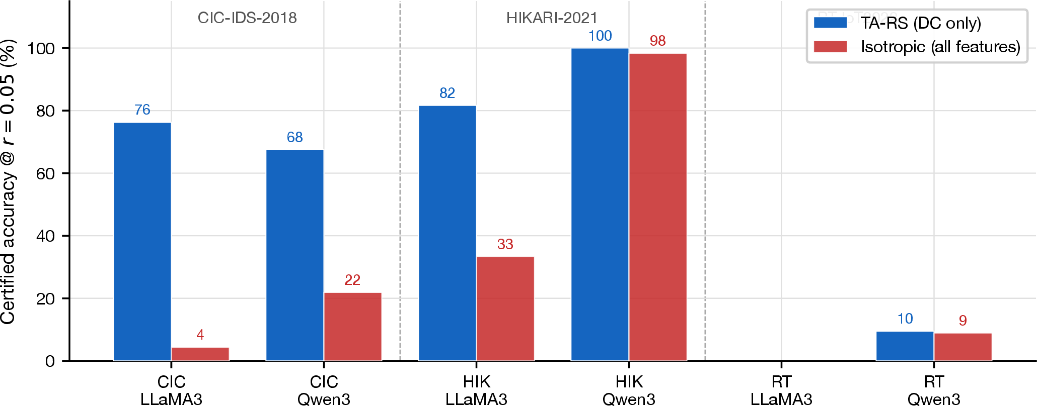
Smoothing support matters. The headline gap at \(r{=}0.05\), \(\sigma{=}0.25\) is \(+72\) pp for CIC/LLaMA3 (TA-RS \(76\%\) vs.isotropic \(4\%\)) and \(+48\) pp for HIKARI/LLaMA3 (\(82\%\) vs.\(33\%\)). Because both methods employ the same DC-noise-augmented model, the gap is a pure test-time smoothing-support effect. The residual advantage against a fairly trained isotropic baseline is \(4\)–\(19\) pp (Table 10). Median radii \(\tilde{R}{=}0.456\) for CIC/LLaMA3 confirm that certified samples sit well above the \(r{=}0.05\) threshold; increasing \(\sigma\) trades CA(0.05) for larger radii (\(\tilde{R}{\approx}0.96\) at \(\sigma{=}1.00\)). HIKARI/Qwen3 reaches \(100\%\) at all \(\sigma\) with zero abstention; HIKARI/LLaMA3 (\(+48\) pp) is the cleaner alignment witness since isotropic RS is not also saturated. Wilson 95% CIs confirm the headline effects are significant: CIC/LLaMA3 TA-RS \(76\%\) [69–82] vs.\(4\%\) [2–9]; HIKARI/LLaMA3 \(82\%\) [74–88] vs.\(33\%\) [25–42]. RT-IoT2022 is the boundary case: both TA-RS and isotropic RS yield \(4\)–\(11\%\) CA (\(\leq 4\) pp gap), showing that alignment has no value when the base model is unstable. Section 6.6 isolates this.
| \(\sigma=0.25\) | \(\sigma=0.50\) | \(\sigma=1.00\) | |||||||
|---|---|---|---|---|---|---|---|---|---|
| 3-5 (lr)6-8 (lr)9-10 Dataset | Model | ||||||||
| \(.05/.15\) | |||||||||
| \(.05\) | \(\Delta\) | ||||||||
| \(.05/.15\) | |||||||||
| \(.05\) | \(\Delta\) | ||||||||
| \(.05/.15\) | SA | ||||||||
| CIC-IDS-2018 | LLaMA3-8B | \(\mathbf{76}/71\) | 4 | \(+72\) | \(\mathbf{79}/75\) | 18 | \(+62\) | \(67/65\) | 78 |
| Qwen3-8B | \(\mathbf{68}/59\) | 22 | \(+46\) | \(\mathbf{71}/66\) | 22 | \(+49\) | \(63/59\) | 74 | |
| LLaMA3-8B | \(\mathbf{82}/70\) | 33 | \(+48\) | \(\mathbf{78}/72\) | 33 | \(+45\) | \(72/70\) | 87 | |
| Qwen3-8B | \(\mathbf{100}/100\) | 98 | \(+2\) | \(\mathbf{100}/100\) | 81 | \(+19\) | \(100/100\) | 100 | |
| LLaMA3-8B | \(4/4\) | \(\mathbf{5}\) | \(-1\) | \(\mathbf{7}/5\) | 5 | \(+1\) | \(8/6\) | 30 | |
| Qwen3-8B | \(\mathbf{10}/4\) | 9 | \(+1\) | \(\mathbf{11}/5\) | 7 | \(+4\) | \(10/8\) | 36 | |
4pt

6.3 Finding 3: Abstention Identifies the Mechanism↩︎
Table 5 asks why threat-aligned smoothing improves certified accuracy on CIC-IDS-2018 and HIKARI-2021. The main mechanism is abstention. For CIC-IDS-2018 / LLaMA3-8B, isotropic RS abstains on \(68\%\) of samples, while TA-RS abstains on only \(8\%\). This \(60\) pp abstention gap accounts for most of the \(72\) pp certified-accuracy gap.
This pattern is consistent with the proposed mechanism. When isotropic noise is injected into UC features (e.g., destination byte counts, server timing statistics), the base classifier—even after noise-augmented training on DC noise—sees feature distributions outside the stability region induced by training. The resulting vote distribution is often too flat for the Clopper–Pearson lower bound to exceed 0.5, so the certification algorithm abstains. TA-RS avoids this failure mode by perturbing only the DC coordinates.
| Dataset | Model | TA-RS | Isotropic |
|---|---|---|---|
| CIC-IDS-2018 | LLaMA3-8B | \(8\) | \(68\) |
| CIC-IDS-2018 | Qwen3-8B | \(14\) | \(44\) |
| HIKARI-2021 | LLaMA3-8B | \(3\) | \(15\) |
| HIKARI-2021 | Qwen3-8B | \(0\) | \(1\) |
| RT-IoT2022 | LLaMA3-8B | \(78\) | \(76\) |
| RT-IoT2022 | Qwen3-8B | \(60\) | \(27\) |
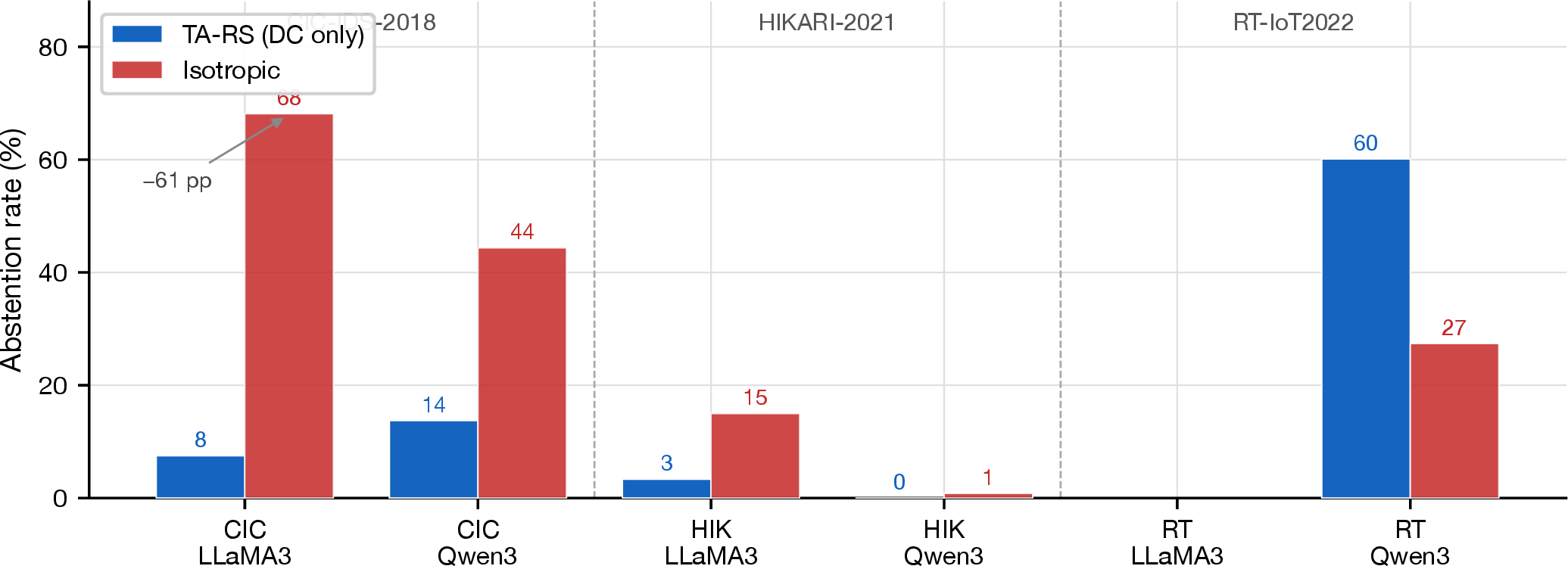
Fig. 4 visualizes the same abstention pattern across all configurations. The figure supports the mechanism claim for CIC and HIKARI, but it also shows the limit of the mechanism: on RT-IoT2022, TA-RS still abstains heavily under the default training recipe.
Smooth accuracy as the stability check. Table 6 asks whether the smoothed classifier remains correct under DC noise before abstention is considered. On CIC-IDS-2018, the noise-augmented TA-RS classifiers maintain \(74\)–\(82\%\) smooth accuracy across the tested \(\sigma\) values, compared with the clean-trained model’s \(\approx 84\%\) clean accuracy prior to noise augmentation. HIKARI / Qwen3-8B retains \(100\%\) smooth accuracy at all \(\sigma\) values, which explains why certification is easy for that pair. RT-IoT2022 has much lower smooth accuracy (\(30\)–\(42\%\)), so its low certified accuracy is not only an abstention problem; the smoothed classifier is often incorrect.
| Dataset | Model | \(\sigma{=}0.25\) | \(\sigma{=}0.50\) | \(\sigma{=}1.00\) |
|---|---|---|---|---|
| CIC-IDS-2018 | LLaMA3-8B | 82 | 81 | 78 |
| CIC-IDS-2018 | Qwen3-8B | 79 | 81 | 74 |
| HIKARI-2021 | LLaMA3-8B | 88 | 87 | 87 |
| HIKARI-2021 | Qwen3-8B | 100 | 100 | 100 |
| RT-IoT2022 | LLaMA3-8B | 36 | 32 | 30 |
| RT-IoT2022 | Qwen3-8B | 42 | 38 | 36 |
| CA(0.05) | CA(0.15) | \(\tilde{R}\) | ||||
|---|---|---|---|---|---|---|
| 3-4(lr)5-6 Dataset / Model | \(\sigma\) | TA | ISO | TA | ISO | (TA) |
| CIC / LLaMA3 | 0.25 | 76 | 4 | 71 | 2 | 0.456 |
| 0.50 | 79 | 18 | 75 | 11 | 0.762 | |
| 1.00 | 67 | 23 | 65 | 21 | 0.958 | |
| HIKARI / Qwen3 | 0.25 | 100 | 98 | 100 | 78 | 0.456 |
| 0.50 | 100 | 81 | 100 | 56 | 0.913 | |
| 1.00 | 100 | 33 | 100 | 33 | 1.826 | |
| RT-IoT / LLaMA3 | 0.25 | 4 | 5 | 4 | 3 | 0.045 |
| 0.50 | 7 | 5 | 5 | 5 | 0.082 | |
| 1.00 | 8 | 6 | 6 | 5 | 0.139 | |
6.4 Certified Accuracy vs.Radius↩︎
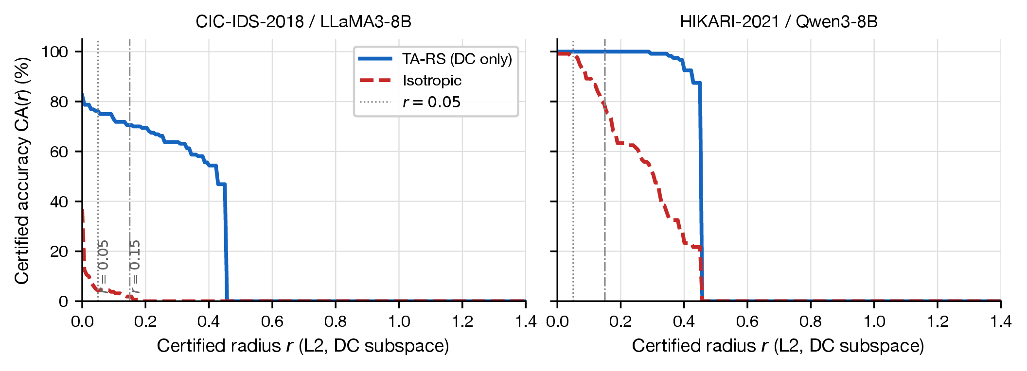
Fig. 5 shows that the \(r{=}0.05\) and \(r{=}0.15\) operating points sit on a stable CA–radius curve, not isolated peaks. For CIC/LLaMA3-8B at \(\sigma{=}0.25\), CA(\(r\)) stays \({\geq}60\%\) through \(r{=}0.30\) and drops sharply only near \(r{\approx}0.46\) (the \(N{=}200\) ceiling \(R_{\max}{\approx}0.453\)). Median radii \(\tilde{R} = 0.34\)–\(0.46\) confirm the certificates have genuine margin above \(r{=}0.05\). The L\(_\infty\)-equivalent conversion (\(\varepsilon\sqrt{|\mathcal{F}_{\mathrm{DC}}|}\)) is in Section 7.2.
6.5 Clean-Robustness Tradeoff↩︎
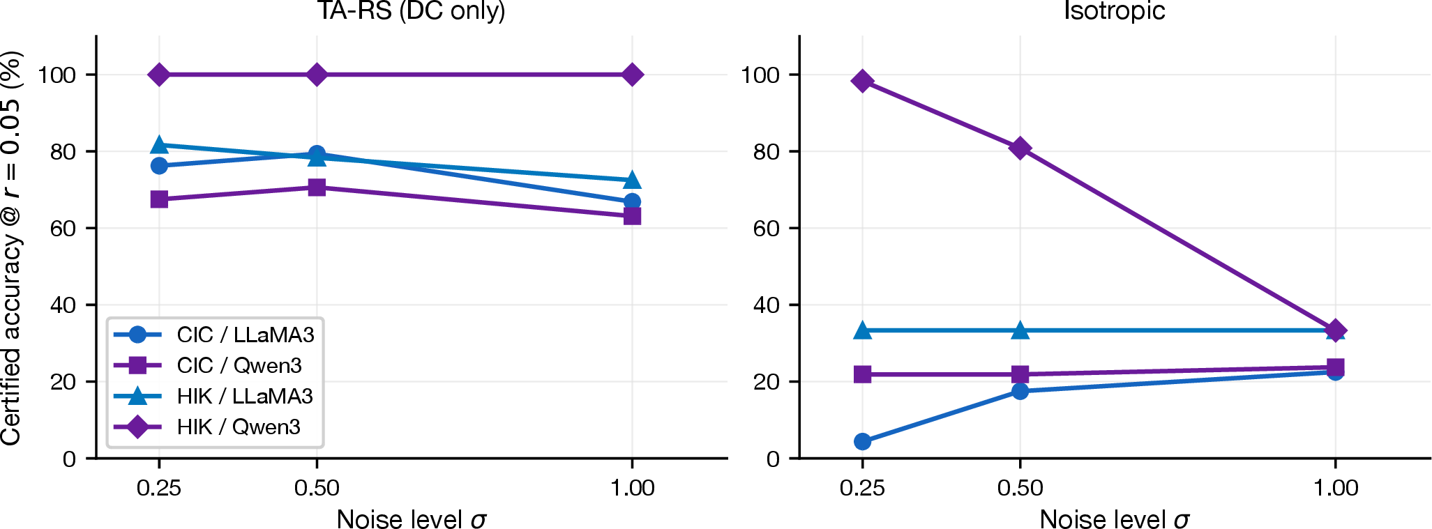
Fig. 6 and Table 7 demonstrate the \(\sigma\) tradeoff: increasing \(\sigma\) expands \(\tilde{R}\) (0.456 \(\to\) 0.958 for CIC/LLaMA3) with mild SA drop (82% \(\to\) 78%), matching the concave RS frontier [10]. CA(0.05) peaks at \(\sigma{=}0.50\) (79%). For HIKARI/Qwen3, TA-RS holds 100% across all \(\sigma\) while isotropic RS falls from 98% to 33%—evidence that full-space noise harms UC-stable datasets. On RT-IoT2022, \(\sigma\) changes add only 4 pp; Section 6.6 isolates the cause.
6.6 RT-IoT2022: Sensitivity to Noise-Augmented Training↩︎
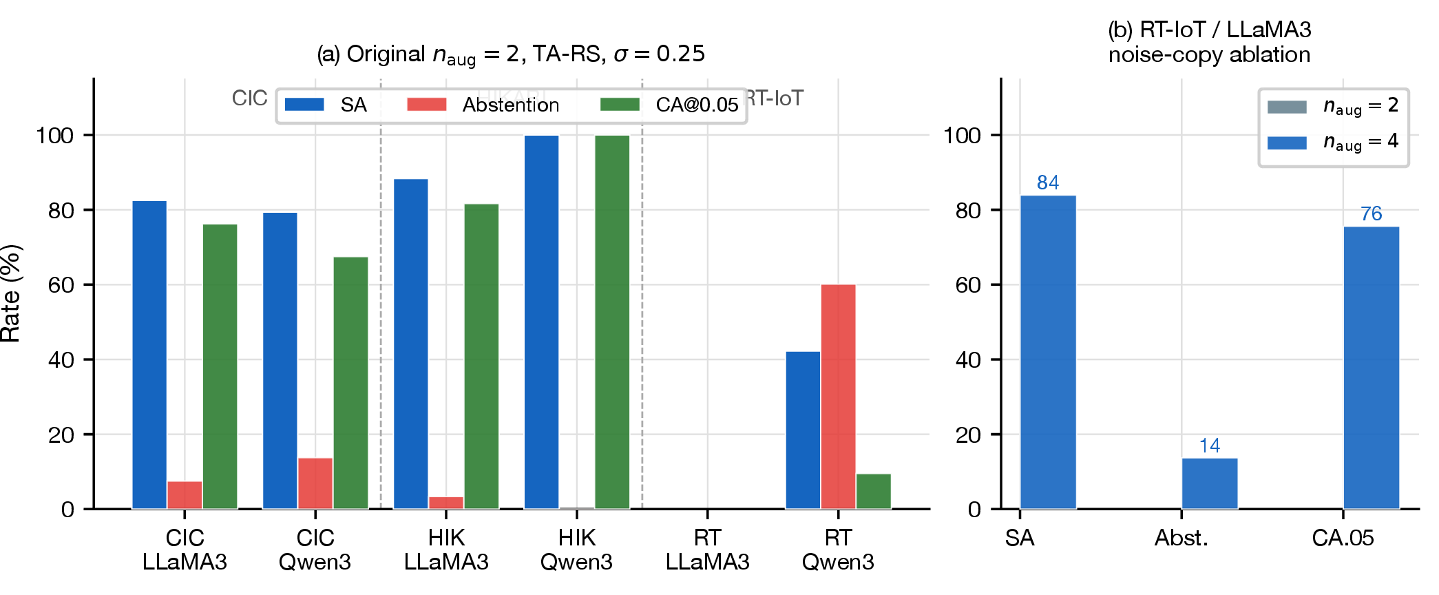
Baseline failure. RT-IoT2022 tests the second condition in the thesis by removing it. With the default noise-copy count (\(n_\text{aug}{=}2\), same as CIC/HIKARI), TA-RS achieves CA(0.05) \(\leq 10\%\) because the LLM does not learn stable predictions under DC noise. For LLaMA3-8B: SA \(=\) \(36\%\) (barely above the \(20\%\) five-class random baseline) and abstention \(=\) \(78\%\). For Qwen3-8B: SA \(=\) \(42\%\) and abstention \(=\) \(60\%\). The TA-vs-ISO gap collapses to \({\leq}1\) pp for both models, indicating that restricting noise to \(\mathcal{F}_{\mathrm{DC}}\) cannot rescue a smoothed classifier whose votes are mostly wrong or inconclusive.
Ablation: noise copy count. We retrain both LLaMA3-8B and Qwen3-8B on all three datasets with \(n_\text{aug}{=}4\) (doubling the number of noise-augmented copies per training sample) and re-certify at \(\sigma{=}0.25\). Table 8 reports SA, abstention, and CA(0.05) for both \(n_\text{aug}\) values across all six (model, dataset) configurations. For RT-IoT2022 with \(n_\text{aug}{=}4\):
SA recovers from \(36\%\)/\(42\%\) to \(\mathbf{83\%}\)/\(\mathbf{70\%}\) (LLaMA3/Qwen3), reaching CIC/HIKARI levels;
abstention drops from \(78\%\)/\(60\%\) to \(\mathbf{12\%}\)/\(\mathbf{3\%}\);
CA(0.05) increases from \(4\%\)/\(10\%\) (Table 4) to \(\mathbf{76\%}\)/\(\mathbf{69\%}\).
| Dataset | Model | \(n_\text{aug}\) | SA / Abstain | CA(0.05) |
|---|---|---|---|---|
| CIC-IDS-2018 | LLaMA3-8B | 2\(^\dagger\) | 82% / 8% | 76% |
| 4 | 74% / 16% | 61% | ||
| CIC-IDS-2018 | Qwen3-8B | 2\(^\dagger\) | 79% / 14% | 68% |
| 4 | 79% / 6% | 74% | ||
| HIKARI-2021 | LLaMA3-8B | 2\(^\dagger\) | 88% / 3% | 82% |
| 4 | 96% / 4% | 88% | ||
| HIKARI-2021 | Qwen3-8B | 2\(^\dagger\) | 100% / 0% | 100% |
| 4 | 100% / 0% | 100% | ||
| RT-IoT2022 | LLaMA3-8B | 2\(^\dagger\) | 36% / 78% | 4% |
| 4 | 83% / 12% | 76% | ||
| RT-IoT2022 | Qwen3-8B | 2\(^\dagger\) | 42% / 60% | 10% |
| 4 | 70% / 3% | 69% |
4pt
Interpretation. The ablation isolates noise-stability as the binding constraint. With \(n_\text{aug}{=}4\), CA rises by \(+72\) pp for LLaMA3 (\(4\% \to 76\%\)) and \(+59\) pp for Qwen3 (\(10\% \to 69\%\)), while the TA-vs-ISO gap remains large (\(+52\)/\(+45\) pp)—DC-alignment continues to matter once the base model is stable. The isotropic aug-4 baseline reaches only SA \(=24\%\) on RT-IoT2022 (barely above the 20% random floor), confirming that full-feature noise augmentation alone cannot substitute for DC-alignment.
A sample-level \(p_A\) diagnostic makes the mechanism concrete. Under \(n_\text{aug}{=}2\), \(78.0\%\) of RT-IoT/LLaMA3 samples have \(p_A\leq 0.5\) (mean \(p_A{=}0.40\))—the smoothed classifier simply does not reach a decisive majority vote. Under \(n_\text{aug}{=}4\), only \(12.5\%\) abstain and \(76.2\%\) reach \(p_A{>}0.8\). By contrast, CIC and HIKARI have abstention rates of \(7.5\%\) and \(3.3\%\) under the default recipe (mean \(p_A{\approx}0.87\) and \(0.86\)), placing the RT-IoT2022 failure squarely in dataset-specific noise instability, not a certificate design flaw.
One boundary condition: CIC/LLaMA3 CA decreases at \(n_\text{aug}{=}4\) (\(76\% \to 61\%\)) as abstention rises from \(8\%\) to \(16\%\), signaling over-regularization. The aug-4 result is therefore diagnostic rather than prescriptive; we do not replace Table 4 with it.
Fig. 7 illustrates the three-way contrast (SA, abstention, CA) for the \(n_\text{aug}{=}2\) configurations and the RT-IoT2022 noise-copy ablation.
6.7 Fair Baseline Comparisons↩︎
The main-table baseline (isotropic RS with DC-trained model) shares the training recipe with TA-RS, isolating the test-time noise-support choice. This section reports two additional baselines needed to rule out confounds: (4) isotropic RS with iso-trained models (training-recipe fairness check) and (5) random-subspace RS (dimensionality-reduction control). Both are required for a complete assessment of whether TA-RS advantages stem from DC-alignment or from some other factor.
Exp A: Random-Subspace RS. To test whether the TA-RS advantage arises purely from using a smaller-dimensional noise subspace (rather than from alignment with attacker-controllable features), we certify the same DC-noise-augmented models with noise restricted to a randomly chosen subspace of size \(|\mathcal{F}_{\mathrm{DC}}|\). If dimensionality reduction alone explained the advantage, random-subspace RS should perform comparably to TA-RS.
Table 9 shows CA(0.05) at \(\sigma{=}0.25\) for TA-RS, random-subspace RS, and isotropic RS (unfair baseline using the same DC-trained model), where CA \(=\) fraction correctly classified AND certified. On CIC-IDS-2018 and HIKARI-2021, TA-RS exceeds random-subspace RS by \(22\)–\(55\) pp, confirming that DC-alignment contributes beyond mere dimensionality reduction. Two patterns in Table 9 deserve closer inspection.
First, HIKARI-2021 / Qwen3-8B shows near-identical performance (TA-RS 100% vs.RandSub 99%), which might seem to weaken the DC-alignment argument. HIKARI has \(|\mathcal{F}_{\mathrm{DC}}|{=}25\) out of \(d{=}82\) total features, so a randomly chosen subspace of size 25 has an expected \(|\mathcal{F}_{\mathrm{DC}}|^2/d \approx 7.6\) features in common with the true DC set—only 30% of the DC features by expectation. The near-tie for Qwen3-8B therefore reflects near-ceiling noise stability of this model on HIKARI: when a model is stable on almost all features, any size-25 subspace tends to yield high CA. The LLaMA3-8B row (TA-RS 82% vs.RandSub 60%), which is not at ceiling, more directly demonstrates the 22 pp DC-alignment advantage.
Second, on RT-IoT2022 (both models), random-subspace RS substantially outperforms TA-RS (\(+47\)–\(66\) pp). This result is a controlled indicator of DC-specific instability, not a general failure of subspace smoothing. RT-IoT2022 has 27 DC features out of 83 total; a random subspace of the same size has an expected overlap of only \(27^2/83 \approx 8.8\) DC features, drawing mostly from IC and UC coordinates for which the model exhibits greater noise stability under default training. The DC subspace is thus the hardest subspace to be noise-stable on for this dataset—precisely the features the attacker controls are the ones the default fine-tuning recipe has not made robust. This confirms that the RT-IoT2022 failure is specifically a DC-feature instability, and motivates the \(n_\text{aug}\) ablation (Section 6.6) as a targeted remedy. To verify robustness to mask choice, we repeat Exp A with 10 independently drawn masks (seeds 99, 101, 103, 107, 109, 113, 131, 137, 139, 149) and report mean CA and 95% CI (Table 9). TA-RS leads RandSub on CIC-IDS-2018 by \(26\pm19\) pp (LLaMA3) and \(30\pm9\) pp (Qwen3); the LLaMA3-8B HIKARI gap is \(26\pm11\) pp. RT-IoT2022 confirms the DC-instability pattern across all 10 seeds, consistent with the noise-stability interpretation.
| Dataset | Model | TA-RS | RandSub\(^\dagger\) | Iso |
|---|---|---|---|---|
| CIC-IDS-2018 | LLaMA3-8B | 76% | 21% | 4% |
| CIC-IDS-2018 | Qwen3-8B | 68% | 29% | 22% |
| HIKARI-2021 | LLaMA3-8B | 82% | 60% | 33% |
| HIKARI-2021 | Qwen3-8B | 100% | 99% | 98% |
| RT-IoT2022 | LLaMA3-8B | 4% | 70% | 5% |
| RT-IoT2022 | Qwen3-8B | 10% | 57% | 9% |
4pt
Exp B: Iso-Trained Baseline. Baseline (2) in the main comparison uses a DC-noise-augmented model with isotropic certification—a training-recipe mismatch that may understate the true isotropic RS performance. To correct for this, we fine-tune separate models using isotropic Gaussian noise augmentation (iso-trained) and certify them with isotropic RS.
Table 10 quantifies the fair-baseline gap for matched \(n_\text{aug}\). Under \(n_\text{aug}{=}2\): TA-RS leads iso-trained RS on CIC (\(+19\) pp/\(+4\) pp for LLaMA3/Qwen3). On HIKARI, iso-trained reaches 99% (near ceiling), ahead of TA-RS for LLaMA3 but matching Qwen3. On RT-IoT2022, iso-trained wins decisively (\(67\%\)/\(60\%\) vs.\(4\%\)/\(10\%\))—because full-feature augmentation incidentally stabilises the base model, not because isotropic noise is traffic-aligned.
To ensure that the RT-IoT2022 comparison at \(n_\text{aug}{=}4\) is also fair, we train iso-trained models with \(n_\text{aug}{=}4\) for all six configurations and certify them. The lower block of Table 10 reports the resulting CA. At \(n_\text{aug}{=}4\), the iso-trained models also improve substantially on RT-IoT2022 (reflecting that more augmentation helps any training recipe), and the table reveals whether the residual TA-RS vs.iso-trained gap persists once augmentation budget is equalised.
| Dataset | Model | TA-RS | Iso-Trained | Iso (unfair) |
|---|---|---|---|---|
| \(n_\text{aug}=2\) (matched augmentation) | ||||
| CIC-IDS-2018 | LLaMA3-8B | 76% | 57% | 4% |
| CIC-IDS-2018 | Qwen3-8B | 68% | 64% | 22% |
| HIKARI-2021 | LLaMA3-8B | 82% | 99% | 33% |
| HIKARI-2021 | Qwen3-8B | 100% | 99% | 98% |
| RT-IoT2022 | LLaMA3-8B | 4% | 67% | 5% |
| RT-IoT2022 | Qwen3-8B | 10% | 60% | 9% |
| \(n_\text{aug}=4\) (matched augmentation) | ||||
| CIC-IDS-2018 | LLaMA3-8B | 61% | 45% | — |
| CIC-IDS-2018 | Qwen3-8B | 74% | 68% | — |
| HIKARI-2021 | LLaMA3-8B | 88% | 99% | — |
| HIKARI-2021 | Qwen3-8B | 100% | 99% | — |
| RT-IoT2022 | LLaMA3-8B | 76% | 58% | — |
| RT-IoT2022 | Qwen3-8B | 69% | 52% | — |
4pt
The two certificates differ in scope: iso-trained RS certifies all \(\mathbb{R}^d\) directions (including IC/UC the attacker cannot modify), while TA-RS is scoped to the DC subspace—the guarantee the traffic threat model actually requires. On CIC/LLaMA3, DC-alignment cuts abstention by \(19\) pp, raising CA even though the iso-trained certificate covers a broader perturbation set. The RT-IoT2022 reversal is a base-model stability failure, not a DC-alignment failure: when noise stability is insufficient, more augmentation (Section 6.6) is the primary lever.
Exp C: Matched random-subspace baseline. Table 10 compares TA-RS against an iso-trained model certified with DC-subspace noise—but DC-subspace certification is itself a deliberate design choice that could be replaced by a randomly chosen \(K\)-dimensional subspace of the same size (\(K{=}|\mathcal{F}_{\mathrm{DC}}|\)). To isolate the effect of subspace selection from that of training-certification matching, we certify the iso-trained models (same checkpoints as Table 10) with \(10\) independently sampled random subspaces of size \(K{=}|\mathcal{F}_{\mathrm{DC}}|\) each. Across six configurations (\(3\) datasets \(\times\) \(2\) models, \(10\) seeds each), the outcome is mixed: DC-subspace certification wins decisively on CIC/Qwen3 (\(\Delta{=}{-13}\) pp vs.random mean) and is within \(1\) pp on HIKARI-2021 (both methods saturate near \(100\%\)); random subspace wins on RT-IoT2022/LLaMA3 (\(\Delta{=}{+20}\) pp, \(|\mathcal{F}_{\mathrm{DC}}|{=}27\)) and CIC/LLaMA3 (\(\Delta{=}{+6}\) pp). Averaged over all six configurations, the mean CA is \(70.0\%\) for DC-cert and \(72.0\%\) for random-cert, a \(2\) pp gap in favour of random—within the seed-to-seed variability of random-subspace itself (std \(1\)–\(9\) pp). The results confirm that neither method dominates numerically; the case for DC selection rests on semantic alignment (the DC subspace corresponds to traffic features the adversary actually controls) and determinism (a fixed, reproducible guarantee rather than a seed-dependent one).
Exp D: Anisotropic RS. Anisotropic Randomized Smoothing [13] generalises the noise distribution by assigning a per-feature variance, potentially improving over the binary \(\sigma_{\mathrm{IC}}{=}0\) choice of TA-RS. To quantify this, we certify the same DC-noise-augmented models under anisotropic noise (\(\sigma_{\mathrm{DC}}{=}0.25\), \(\sigma_{\mathrm{IC/UC}}{=}0.05\)) while retaining the DC-subspace certificate formula. Table 11 reports CA(0.05) at \(\sigma{=}0.25\).
| Dataset | Model | TA-RS | Aniso-RS |
|---|---|---|---|
| CIC-IDS-2018 | LLaMA3-8B | 76% | 78% |
| CIC-IDS-2018 | Qwen3-8B | 68% | 67% |
| HIKARI-2021 | LLaMA3-8B | 82% | 83% |
| HIKARI-2021 | Qwen3-8B | 100% | 100% |
| RT-IoT2022 | LLaMA3-8B | 76% | 74% |
| RT-IoT2022 | Qwen3-8B | 69% | 69% |
4pt
Aniso-RS and TA-RS differ by at most 2 pp across all six configurations (absolute differences: \(\{+2, -1, +2, 0, -2, 0\}\) pp), well within the Monte Carlo sampling error at \(N{=}200\) (one misclassified sample \(\approx 2.5\) pp). This confirms two things: (i) DC-noise-augmented training produces a model robust enough that small IC/UC perturbations at certification time do not materially change pA; and (ii) the design choice \(\sigma_{\mathrm{IC}}{=}0\) in TA-RS is principled (no wasted noise budget on non-attacker-controllable features) rather than a sensitive hyperparameter—a data-driven anisotropic baseline with \(\sigma_{\mathrm{IC}}{=}0.05\) achieves no advantage over our semantically motivated choice.
6.8 Finding 4: Empirical Robustness Is Consistent with the Certified Bound↩︎
A core soundness requirement of randomized smoothing is that the certified accuracy should behave as a conservative lower bound under fixed empirical attacks. Table 12 asks whether the reported certificates are consistent with A1-style transfer attacks (PGD [2], [28] on an XGBoost surrogate; [1]) against the noise-augmented TA-RS classifier. This experiment is a consistency check, not a replacement for the formal guarantee.
Protocol. We sample \(N_{\text{smooth}}{=}20\) DC-noise copies per test point (\(\sigma{=}0.25\)) and take the majority vote as the smoothed prediction. Transfer attacks are generated at \(\varepsilon \in \{0.05, 0.15\}\) (L\(_\infty\), DC features). We report attack success rate (ASR) conditional on clean-correct samples, and compute empirical robustness as \(1{-}\text{ASR}_{\text{smoothed}}\).
| Dataset | \(\varepsilon\) | ASR\(_{\text{base}}\) | ASR\(_{\text{smooth}}\) | Gain | Emp. Rob. | CA\((r{=}\varepsilon)\) |
|---|---|---|---|---|---|---|
| CIC / Qwen3 | 0.05 | 16.0% | 8.6% | \(+\)7.4pp | 91.4% | 67.5% \(✔\) |
| CIC / Qwen3 | 0.15 | 19.1% | 8.6% | \(+\)10.5pp | 91.4% | 59.4% \(✔\) |
| HIKARI / LLaMA3 | 0.05 | 3.9% | 1.6% | \(+\)2.4pp | 98.4% | 81.7% \(✔\) |
| HIKARI / LLaMA3 | 0.15 | 4.7% | 0.0% | \(+\)4.7pp | 100.0% | 70.0% \(✔\) |
2.5pt
Three observations follow from Table 12. First, empirical robustness exceeds the reported L2 certified accuracy in every row. Note that these metrics have different denominators: empirical robustness is conditioned on clean-correct predictions, while CA\((r)\) is unconditional (penalising both misclassification and abstention). The observed ordering is therefore partially structural and does not by itself validate certificate soundness; it is consistent with—but not proof of—conservativeness. Additionally, the L\(_\infty\)/L2 norm mismatch means the two columns represent different threat sets. Second, the smoothed classifier reduces ASR beyond the base model in every measured case: the average reduction is \(7.5\) pp on CIC and \(3.6\) pp on HIKARI. Third, the margin between empirical robustness and certified accuracy is large (up to \(30\) pp on HIKARI), indicating that the Clopper–Pearson bound with \(N{=}200\) is conservative. Increasing \(N\) would tighten this gap without changing the empirical defense quality.
7 Discussion↩︎
7.1 Certified vs.Empirical Robustness↩︎
Table 12 is a consistency check, not a replacement for the certificate. The smoothed classifier reduces transfer-attack ASR on CIC and HIKARI; empirical robustness exceeds certified accuracy by \(16\)–\(32\) pp, as expected for a conservative Clopper–Pearson bound. An empirical ASR reduction cannot be extrapolated to attacks outside the certified L2 ball, and it does not address the L2/L\(_\infty\) norm gap discussed next.
7.2 The L2/L\(_\infty\) Norm Gap↩︎
The most important boundary condition is the norm mismatch. The TA-RS certificate is stated in L2 norm, while A1 threat budgets are specified as L\(_\infty\). A reported L2 threshold \(r{=}0.05\) therefore does not by itself certify the full L\(_\infty\) budget \(\varepsilon{=}0.05\) over all DC coordinates. The direct conversion is \(R \geq \varepsilon\sqrt{|\mathcal{F}_{\mathrm{DC}}|}\). For \(\varepsilon{=}0.05\), this threshold is \(0.187\) for CIC-IDS-2018 (\(|\mathcal{F}_{\mathrm{DC}}|{=}14\)), \(0.250\) for HIKARI-2021 (\(|\mathcal{F}_{\mathrm{DC}}|{=}25\)), and \(0.260\) for RT-IoT2022 (\(|\mathcal{F}_{\mathrm{DC}}|{=}27\)).
Table 13 reports the fraction of samples that are both correct and certified at \(R_\infty\) for each dataset and model, at \(\sigma{=}0.25\). On CIC-IDS-2018 and HIKARI-2021 (main recipe, \(n_\mathrm{aug}{=}2\)), coverage ranges from 55–100%. RT-IoT2022 with \(n_\mathrm{aug}{=}4\) achieves 65% on both models—comparable to CIC/HIKARI—confirming that the L\(_\infty\)-equivalent coverage is primarily limited by base model stability, not by the norm conversion. These values demonstrate that the L2 certificate covers the small-budget L\(_\infty\) threat model for a substantial fraction of samples on all three datasets, but they should not be described as full coverage.
| Dataset | Model | \(R_\infty\) | CA@0.05 | CA@\(R_\infty\) |
|---|---|---|---|---|
| CIC-IDS-2018 | LLaMA3-8B | 0.187 | 76.2% | 69.4% |
| CIC-IDS-2018 | Qwen3-8B | 0.187 | 67.5% | 55.0% |
| HIKARI-2021 | LLaMA3-8B | 0.250 | 81.7% | 65.0% |
| HIKARI-2021 | Qwen3-8B | 0.250 | 100.0% | 100.0% |
| RT-IoT2022 | LLaMA3-8B | 0.260 | 75.6%\(^\dagger\) | 65.5%\(^\dagger\) |
| RT-IoT2022 | Qwen3-8B | 0.260 | 69.0%\(^\dagger\) | 64.9%\(^\dagger\) |
4pt
\(\dagger\) \(n_\mathrm{aug}{=}4\) checkpoint.
Developing a provably correct native L\(_\infty\) certificate for multi-dimensional DC-subspace uniform noise—accounting for the dimension-dependent overlap structure of the hypercube smoothing distribution—remains an open problem and a direction for future work.
7.3 Effect of Monte Carlo Budget (\(N\))↩︎
Table 14 compares \(N{=}200\) against \(N{=}1{,}000\) for all six headline configurations (\(\sigma{=}0.25\)), with \(N{=}200\) subsampled from the same noise realization to eliminate seed variance. CA gain is \(0\)–\(4.1\) pp (mean \(1.2\) pp); five of six rows change by \(\leq 1.2\) pp. The largest shift is HIKARI/LLaMA3 (\(+4.1\) pp), where borderline samples are promoted; ranking and gap structure are fully preserved. Larger \(N\) tightens the Clopper–Pearson bound but cannot recover stability absent in the base model.
| Dataset | Model | CA(%) | Abstain(%) | ||
|---|---|---|---|---|---|
| 3-4(lr)5-6 | \(N{=}200\) | \(N{=}1000\) | \(N{=}200\) | \(N{=}1000\) | |
| CIC-IDS-2018 | LLaMA3-8B | 77.5 | 77.5 | 9.4 | 8.8 |
| CIC-IDS-2018 | Qwen3-8B | 67.5 | 68.1 | 23.1 | 17.5 |
| HIKARI-2021 | LLaMA3-8B | 81.7 | 85.8 | 9.2 | 4.2 |
| HIKARI-2021 | Qwen3-8B | 100.0 | 100.0 | 0.0 | 0.0 |
| RT-IoT2022 | LLaMA3-8B | 76.2 | 77.4 | 14.9 | 13.1 |
| RT-IoT2022 | Qwen3-8B | 69.0 | 69.0 | 3.0 | 3.0 |
RT-IoT2022 rows: \(n_\text{aug}{=}4\) checkpoint.
7.4 Discrete DC Features↩︎
Section 4 establishes that the clip operation is absorbed into the base classifier, so Theorem 2 holds exactly. To summarize the certificate scope for discrete feature types: for count-valued DC features, the normalization step size \(\Delta_i \leq 10^{-4}\) is negligible relative to \(\sigma{=}0.25\), so Theorem 2 applies with negligible rounding effect. For binary flag features, the certified radii \(r \leq 0.15\) are strictly below the rounding threshold \(0.5\), making the continuous certificate conservative: the stated L2 bound understates true robustness for the binary flag dimensions because no adversary within budget can deterministically flip a flag. A fully rigorous certificate for mixed discrete-continuous features would employ discrete smoothing distributions [8], which we leave as future work.
7.5 TA-RS on Non-LLM Tabular Classifiers↩︎
A natural question is whether the traffic-aware mechanism is LLM-specific or whether it also benefits classical tabular classifiers such as XGBoost [29] and LightGBM [30]. We apply TA-RS and isotropic RS to these two models (trained without noise augmentation, CPU-only) at \(\sigma{=}0.25\) and report CA(0.05) in Table 15.
| Dataset | Model | TA-RS | Isotropic |
|---|---|---|---|
| CIC-IDS-2018 | XGBoost | 53% | 73% |
| CIC-IDS-2018 | LightGBM | 37% | 17% |
| HIKARI-2021 | XGBoost | 67% | 73% |
| HIKARI-2021 | LightGBM | 80% | 87% |
| RT-IoT2022 | XGBoost | 74% | 3% |
| RT-IoT2022 | LightGBM | 67% | 18% |
4pt
Table 15 shows no consistent TA-RS advantage when classifiers are trained without noise augmentation. The TA-vs-ISO direction is inconsistent across datasets and models (e.g., TA\(>\)Iso for RT-IoT2022/XGBoost, TA\(<\)Iso for CIC/XGBoost). Without DC-noise augmented training, tree ensembles are unstable under any input noise, and certified accuracy is dominated by abstention rather than noise-subspace choice.
For LLM-IDS, the pattern reinforces the noise-stability requirement: without DC-noise-augmented fine-tuning, neither TA-RS nor isotropic RS produces consistently useful certified accuracy for the evaluated LLMs. Tree ensembles demonstrate a different pattern—RT-IoT/XGBoost (\(74\%\)) and HIKARI/LightGBM (\(80\%\)) achieve non-trivial CA without noise augmentation, consistent with tree classifiers’ greater tolerance for continuous input perturbations. The noise-stability requirement is therefore specific to LLM-based classifiers, not a universal property of randomized smoothing.
7.6 Cross-Domain Boundary Analysis↩︎
A natural question is whether LLM-IDS can be reused across datasets without retraining. Tabular models such as XGBoost make this structurally impossible: a model trained on CIC-IDS-2018 (\(|\text{feat}|=25\)) cannot process HIKARI-2021 inputs (\(|\text{feat}|=82\)) due to feature-dimension mismatch. An LLM accepts arbitrary serialized text, so it can be executed cross-domain; the question is whether this structural executability yields meaningful certified accuracy.
To test whether structural executability translates to meaningful certified accuracy, we evaluate LLaMA3-8B (noise-augmented, \(\sigma{=}0.25\), \(n_\mathrm{aug}{=}4\)) zero-shot on a held-out dataset. Two directions are evaluated: (X1) HIKARI-2021-trained model on CIC-IDS-2018 (restricted to the three shared classes: Normal, CredentialAccess, Exploitation); and (X2) CIC-2018-trained model on HIKARI-2021. Both models receive the target dataset’s serialized feature text at test time.
| Exp | Source\(\to\)Target | Model | SA | CA@0.05 | Abstain |
|---|---|---|---|---|---|
| X1 | HIKARI\(\to\)CIC (3 cls) | LLaMA3-8B | 33.3 | 33.3 | 0.0 |
| X2 | CIC\(\to\)HIKARI | LLaMA3-8B | 33.3 | 33.3 | 0.0 |
| – | CIC\(\to\)HIKARI | NAXGB | structurally infeasible | ||
| – | HIKARI\(\to\)CIC | NAXGB | structurally infeasible | ||
4pt
Table 16 presents the results. Both directions yield near-chance accuracy (\(33.3\%\) SA and CA on 3 classes, abstain \(0\%\)): the model is always confident but matches the random baseline. This outcome traces to dataset-specific feature serialization: the HIKARI-trained model learned to classify 82-feature HIKARI text, while CIC test inputs arrive with 25 different feature names and value ranges—an out-of-distribution prompt that the model cannot resolve beyond chance. The same logic applies to X2. The cross-domain result is therefore negative: pretrained LLM-IDS knowledge does not transfer without dataset-specific fine-tuning. Dataset-agnostic serialization schemes that could enable meaningful cross-domain generalization remain an open problem. The structural executability distinction from NAXGB (which cannot accept inputs of a different feature dimension at all) is architecturally real but operationally moot at chance accuracy.
7.7 Limitations↩︎
Statistical budget, per-class breakdown, and training variance. Certification uses \(N{=}200\) MC samples; the \(N{=}200\) vs.\(N{=}1{,}000\) comparison (Table 14) shows \(\leq 4.1\) pp CA gain (mean \(1.2\) pp), confirming near-convergence when the base model is noise-stable. Test sets employ 40 samples per class; this limits per-class Wilson intervals to \(\pm 15\) pp. Per-class CA(0.05) at \(\sigma{=}0.25\) shows malicious-class CA meeting or exceeding the aggregate on stable datasets: CIC malicious avg \(82\%\)/\(73\%\) (LLaMA3/Qwen3) vs.aggregate \(76\%\)/\(68\%\); HIKARI malicious avg \(72\%\)/\(100\%\); RT-IoT (\(n_\text{aug}{=}4\)) malicious avg \(71\%\)/\(63\%\) with within-class variation (\(18\)–\(100\%\)) driven by class-specific noise stability. All LLM fine-tuning uses a single LoRA seed (42); training variance across seeds was not estimated. Differences below approximately 4–5 pp should therefore be interpreted cautiously: the MC certification measurement itself carries a per-class CI of \(\pm 15\) pp at \(N{=}200\), and LoRA fine-tuning variance is an additional uncharacterised source of uncertainty. The 10-seed random-subspace analysis (Section 6.7) quantifies mask-selection variance but does not substitute for training-seed variance.
RT-IoT2022 sensitivity. The default failure (\(n_\text{aug}{=}2\): CA \(4\%\)/\(10\%\)) is real. The aug-4 ablation and iso-trained baselines both confirm noise-stability—not DC-alignment design—as the operative variable; traffic-aware certification cannot compensate for an unstable base model.
Data quality and scope. CIC-IDS-2018 has \(33.3\%\) train-test overlap [31]; a deduplication audit on our 160-sample evaluation subset finds \(22\) duplicate feature vectors (\(13.8\%\)); their removal shifts CA by at most \(1.6\) pp (LLaMA3: \(76.2\%\!\to\!76.1\%\); Qwen3: \(67.5\%\!\to\!65.9\%\)), so reported values are not materially inflated. HIKARI-2021 has \(2\) duplicates (\(1.7\%\), \(\Delta\leq0.5\) pp); RT-IoT2022 has no duplicate feature vectors. NSL-KDD and UNSW-NB15 are excluded because their categorical encodings create a perturbation-budget mismatch; extending the DC/IC/UC taxonomy to handle encodings is future work. Certification requires \(N{=}200\) forward passes per query, ruling out real-time deployment; offline certification and bound distillation are left to future work. Extension to consistency-regularised certified training (e.g., MACER [32], SmoothAdv [10]) at LLM scale remains open: the per-sample adversarial step required by these methods is prohibitively expensive for 8B-parameter models.
8 Conclusion↩︎
TA-RS shows that certification for LLM-based intrusion detection is not only a matter of applying randomized smoothing to a trained classifier. The certificate is meaningful only when the smoothing distribution matches the attacker’s directly controllable traffic features and the LLM remains stable under noise in that subspace. TA-RS operationalizes this view by smoothing over \(\mathcal{F}_{\mathrm{DC}}\) and certifying the resulting smoothed classifier in the same subspace.
The experiments quantify both conditions. Noise-augmented fine-tuning raises CA from 14–57% (clean-trained) to 68–100% on CIC/HIKARI; traffic-aware smoothing eliminates abstention on non-controllable noise directions (68%\(\to\)8% on CIC/LLaMA3), adding up to 72 pp over isotropic RS applied to the same DC-trained model; the residual advantage over a fairly iso-trained baseline is 4–19 pp on CIC-IDS-2018. At the L\(_\infty\)-equivalent threshold \(R_\infty{=}\varepsilon\sqrt{|\mathcal{F}_{\mathrm{DC}}|}\) (\(\varepsilon{=}0.05\)), 55–100% of CIC/HIKARI samples are certified, with median radii \(1.8\)–\(5{\times}\) above \(R_\infty\) (across \(\sigma{=}0.25\)–\(1.00\)). The RT-IoT2022 boundary condition—where the same default recipe fails—responds directly to additional noise augmentation (\(n_\text{aug}{=}4\): CA \(4\%/10\% \to 76\%/69\%\)), confirming that noise-stability, not DC-alignment design, is the variable that governs the hard cases.
The cross-domain boundary analysis (Table 16) shows that structural executability does not substitute for dataset-specific fine-tuning: zero-shot transfer achieves near-chance certified accuracy, confirming that LLM pretraining knowledge does not transfer to new traffic distributions without fine-tuning. Limitations and future directions are discussed in Section 7.7.
CRediT authorship contribution statement↩︎
Zhenpeng Li: Conceptualization, Methodology, Software, Formal analysis, Investigation, Data curation, Writing – original draft, Writing – review & editing, Visualization.
Declaration of competing interest↩︎
The author declares that he has no known competing financial interests or personal relationships that could have appeared to influence the work reported in this paper.
Data availability↩︎
CIC-IDS-2018, HIKARI-2021, and RT-IoT2022 are publicly available benchmark datasets. Feature annotations, certification code, and per-sample predictions will be released upon acceptance (DOI to be assigned).
Declaration of Generative AI and AI-assisted technologies in the writing process↩︎
During the preparation of this work the author used Claude (Anthropic) to assist with manuscript organisation, language editing, and drafting support. The author reviewed and edited all content as needed and takes full responsibility for the content of the publication.