Independent Sets in Multiset Profile Graphs via Weighted Local Covers
July 15, 2026
1 Introduction↩︎
The spreading number \(\alpha_q(d)\) is the largest size of a family of size-\(d\) multiset profiles over \(q\) symbols in which no two profiles differ by replacing one occurrence of one symbol by another. Equivalently, it is the independence number of the unit-transfer graph on weak compositions of \(d\). The natural cyclic coloring gives, for prime \(q\), an independent checksum fiber of size \[\left\lceil\frac{1}{q}\binom{d+q-1}{q-1}\right\rceil.\] The prime-checksum conjecture asserts that this construction is optimal for all sufficiently large \(d\) and is the central problem of the paper.
Conjecture 1 (Prime-alphabet checksum optimality). For every prime \(q\), there is an integer \(d_0(q)\) such that \[\alpha_q(d)= \left\lceil\frac{1}{q}\binom{d+q-1}{q-1}\right\rceil \qquad(d\geqslant d_0(q)).\]
Under the correspondence \(a\leftrightarrow x_1^{a_1}\cdots x_q^{a_q}\), the same graph is the graph on degree-\(d\) monomials studied by Geramita, Gregory, and Roberts, who determined the classical cases \(q=3\) and \(q=4\) [1]. Subsequent work developed the spreading and covering parameters further [2], [3]. Machacek later studied uniqueness and rigidity of maximum independent sets [4]. These cases have special low-dimensional structure. In three variables the simplex is planar and its boundary consists of one-dimensional paths; in four variables a parity decomposition remains available. The known arguments exploit precisely these features.
The cases \(q=5\) and \(q=7\) are harder because their profile simplices have dimensions four and six. The recurrences used in dimensions two and three no longer control the boundary. Our method covers the graph by translated smaller graphs with known independence numbers. The weight of a translate depends only on a capped version of its anchor profile. This leaves a finite system of linear inequalities, even though the result applies to every large \(d\).
Our principal results prove the prime-checksum conjecture for the next two prime alphabets. For both \(q=5\) and \(q=7\) we obtain \[\alpha_q(d)=\left\lceil\frac{1}{q}\binom{d+q-1}{q-1}\right\rceil \label{eq:intro-q5-q7-main}\tag{1}\] apart from a few low degrees, whose exact values are determined in the corresponding sections. Thus both spreading numbers are completely determined, and the first unresolved odd-prime case is \(q=11\). The same method also gives new unified graph-theoretic proofs of the known three- and four-variable results.
| \(q\) | degrees in which the checksum formula holds | exceptions |
|---|---|---|
| 3 | all \(d\notin\{2,4\}\) | \(\alpha_3(2)=3\), \(\alpha_3(4)=6\) |
| 5 | all \(d\notin\{2,4\}\) | \(\alpha_5(2)=5\), \(\alpha_5(4)=16\) |
| 7 | all \(d\notin\{2,3,4,6\}\) | \(\alpha_7(2)=7\), \(\alpha_7(3)=14\), \(\alpha_7(4)=35\), \(\alpha_7(6)=133\) |
Through the multiplicity-vector correspondence, these independent-set theorems also determine optimal one-deletion-correcting multiset codes for alphabet sizes five and seven, while recovering the known sizes for three and four symbols; see [5] for the broader coding framework. When \(d\) is fixed and \(q\) grows, profiles fall into finitely many partition types. Working with these types solves the degree-five problem for all \(q\geqslant 7\), gives exact infinite families for power-of-two values of \(q\) when \(d\in\{6,8,10\}\), and gives an asymptotically sharp upper bound with three explicit terms for every fixed \(d\geqslant 7\).
1.0.0.1 Organization of the paper.
Section 2 defines the discrete simplex, the unit-transfer graph, the additive colorings that provide independent sets, and the translated local tiles used for upper bounds. Section 3 proves the weighted local-cover inequality and the finite-state reduction: for a fixed tile family, infinitely many vertex-covering conditions are reduced to one finite rational linear system using capped anchor profiles. Sections 4 and 5 apply the method to the known three- and four-variable cases. The first uses translated triangular templates and a planar boundary correction; the second separates odd and even degrees and combines parity with exact-density tiles. These sections provide new proofs of the earlier formulas and illustrate the two basic forms of the method. Section 6 treats five variables using only translated full simplices. It constructs one finite-state certificate for all sufficiently large degrees, checks the remaining finite range, and obtains the exact value for every degree. Section 7 first explains why the simpler tile family handles only an infinite subfamily, then introduces the additional boundary tiles needed for all large degrees and completes the exact seven-variable result with finite checks for the remaining degrees. Section 8 determines the sizes of the additive color classes for cyclic and more general finite abelian label groups. It also states the proposed extension of the finite-tile method to further fixed alphabets. Section 9 turns to the opposite regime, in which \(d\) is fixed and \(q\) grows. It derives the partition-orbit linear program, solves degree five, proves the power-of-two families in degrees six, eight, and ten, records the point at which the simpler clique family stops working, and proves the improved three-term asymptotic upper bound for every fixed \(d\geqslant 7\). Finally, Section 10 gives the multiset-deletion interpretation, summarizes the main results, and lists the remaining open problems.
2 Multiset profile graphs, additive colorings, and local templates↩︎
Throughout, \(q\geqslant 2\) is the number of symbols and \(d\geqslant 0\) is the multiset size. We write \([q]=\{1,\ldots,q\}\), and let \(e_1,\ldots,e_q\) be the standard unit vectors of \(\mathbb{Z}^q\).
Definition 1 (Profile graph). A size-\(d\) multiset profile over \(q\) symbols is a vector in \[\Delta_q(d)=\left\{a\in\mathbb{Z}_{\geqslant 0}^q:\sum_{i=1}^q a_i=d\right\}, \qquad |\Delta_q(d)|=\binom{d+q-1}{q-1}.\] The profile graph \(G_q(d)\) has vertex set \(\Delta_q(d)\); distinct profiles \(a,b\) are adjacent exactly when \(a-b=e_i-e_j\) for some \(i\ne j\), equivalently when \(\lVert a-b\rVert_1=2\). We write \[\alpha_q(d)=\alpha(G_q(d)).\]
The map \(a\mapsto x_1^{a_1}\cdots x_q^{a_q}\) identifies \(G_q(d)\) with the degree-\(d\) monomial graph from the algebraic literature. We use this interpretation only when comparing with earlier work; all arguments below are stated in terms of profiles.
Figure 1 shows this correspondence in the smallest triangular example. The three corners are the pure powers, and moving along an edge transfers one unit of exponent from one variable to another.
![Figure 1: The profile simplex G_3(3) with vertices written as degree-threemonomials; compare [4].](/article/2607.13733/_pdflatex/zaqreydu.png "fig:")
For the basic lower bound, let \(A\) be an abelian group of order \(q\) and label the coordinates by its distinct elements \(g_1,\ldots,g_q\). Color a profile by \[\chi(a)=\sum_{i=1}^q a_i g_i, \qquad a\in\Delta_q(d). \label{eq:additive-coloring}\tag{2}\] For \(s\in A\), let \[I_s(d)=\{a\in\Delta_q(d):\chi(a)=s\}.\] The cyclic specialization takes \(A=\mathbb{Z}_q\) and \(g_i=i-1\). We write \[\sigma_q(a)=\sum_{i=1}^q(i-1)a_i\pmod q \label{eq:cyclic-checksum}\tag{3}\] and denote its fibers by \[\mathcal{C}_{q,d}(r)=\{a\in\Delta_q(d):\sigma_q(a)=r\}, \qquad N_r^{(q)}(d)=|\mathcal{C}_{q,d}(r)|. \label{eq:checksum-classes}\tag{4}\]
If \(a-b=e_i-e_j\) with \(i\ne j\), then \(\chi(a)-\chi(b)=g_i-g_j\ne0\). Thus \(\chi\) is a proper \(q\)-coloring and each fiber is independent. Since the fibers partition \(\Delta_q(d)\), \[\alpha_q(d)\geqslant \left\lceil\frac{1}{q}\binom{d+q-1}{q-1}\right\rceil. \label{eq:additive-lower-bound}\tag{5}\]
For three variables these fibers give the familiar periodic pattern in the triangular grid. The classical proofs for three and four variables and the uniqueness results of Machacek show that the decisive issue is how this interior pattern meets the boundary [1], [4]. Translated induced subgraphs are particularly well suited to that boundary problem. Their local independence numbers are unchanged, while their incidences are governed by exponent arithmetic. These translations take place in the semigroup \(\mathbb{Z}_{\geqslant 0}^q\), not in a quotient group. Let \(H=G_q(r)[U]\) be an induced subgraph of \(G_q(r)\), with \(U\subseteq\Delta_q(r)\), and let \(b\in\Delta_q(d-r)\). The translate of \(H\) by \(b\) is \[b+H:=G_q(d)[b+U], \qquad b+U=\{b+h:h\in U\}.\] When used in a covering argument, this translated copy is a local tile. The purpose of these tiles is to turn a known small independence number into a local upper bound inside the large graph. The map \(h\mapsto b+h\) is a graph isomorphism because translation preserves differences of exponent vectors. Hence \[\alpha(b+H)=\alpha(H). \label{eq:translate-preserves-alpha}\tag{6}\] For every independent set \(I\subseteq G_q(d)\), \[|I\cap V(b+H)|\leqslant\alpha(H). \label{eq:local-tile-bound}\tag{7}\] The next section combines many inequalities of this form. If their weighted sum counts every ambient vertex at least once, it gives an upper bound on the size of every independent set and hence on \(\alpha_q(d)\).
Three templates recur below. The upward simplex \(b+\Delta_q(1)=\{b+e_i:i\in[q]\}\) is a \(K_q\); a translated full simplex \(b+\Delta_q(r)\) is a copy of \(G_q(r)\); and reflected sets of the form \(b+\{\mathbf{1}-e_i:i\in[q]\}\) are again \(q\)-cliques. Theorem 4 applies to every finite family of such shapes. The next sections use full simplices, the two clique orientations, and a small number of boundary-correcting templates.
3 Finite-state weighted local decompositions↩︎
The small graph and its position in the ambient simplex play different roles. A base tile is a fixed finite graph \(H=G_q(r)[U]\) inside the small simplex \(\Delta_q(r)\). For every anchor \(a\in\Delta_q(d-r)\), the translate \(a+H=G_q(d)[a+U]\) places the same shape at a new position in the larger simplex. Thus a finite tile is moved throughout the ambient space by varying \(a\); a weighted tiling assigns weights to these translated copies, which may overlap and need not form a partition. Choosing the base tiles is not automatic. Full simplices suffice in the three- and five-variable arguments, the four-variable argument also needs the two clique orientations, and the seven-variable argument requires mixed profile layers near the boundary. The finite-state theorem does not discover these shapes: once they are chosen, it reduces the search for weights to a finite system, and the later sections show that the stated choices give the required bounds. To separate this universal covering argument from the particular geometry, let \(G=(V,E)\) be a finite graph and let \(\mathcal{T}\) be a finite indexed family of induced subgraphs of \(G\). Its members are the placed tiles; they may overlap, need not be cliques, and need not be mutually isomorphic. No algebraic condition is imposed: for every subset \(W\subseteq V\), the induced graph \(G[W]\) is an admissible tile. In particular, a tile need not be a coset, a simplex, an orbit, or a member of a partition. In the profile-graph applications we choose translates of algebraically structured subsets because their independence numbers and incidences can be controlled; this is a feature of our constructions, not a hypothesis of the local-cover bound. Assign a nonnegative weight \(w_T\) to every \(T\in\mathcal{T}\). The coverage of a vertex and the independence cost are \[F(x)=\sum_{T\in\mathcal{T}}w_T\mathbf{1}_{V(T)}(x), \qquad \mathop{\mathrm{cost}}(\mathcal{T},w)=\sum_{T\in\mathcal{T}}w_T\alpha(T).\] Here \(F(x)\) is simply the total weight of the placed tiles that contain \(x\). It is the bookkeeping tool that turns the local inequalities into the desired global upper bound: the condition \(F(x)\geqslant 1\) ensures that every vertex of an independent set is counted with total weight at least one, while \(\mathop{\mathrm{cost}}(\mathcal{T},w)\) is the resulting upper-bound cost. The weighted family is a fractional local cover when \(F(x)\geqslant 1\) for all \(x\in V\). Thus a correct choice of tile shapes and weights that gives \(F\geqslant 1\) at the target cost is exactly a solution of the upper-bound problem; the fixed-alphabet sections construct such choices.
Theorem 2 (Weighted local-cover bound). Every fractional local cover of \(G\) satisfies \[\alpha(G)\leqslant\sum_{T\in\mathcal{T}}w_T\alpha(T).\] For a fixed template family, the best bound of this form is the value of \[\begin{align} \text{minimize}\quad&\sum_{T\in\mathcal{T}}\alpha(T)w_T,\\ \text{subject to}\quad& \sum_{\substack{T\in\mathcal{T}\\x\in V(T)}}w_T\geqslant 1 &&(x\in V),\\ &w_T\geqslant 0&&(T\in\mathcal{T}). \end{align} \label{eq:abstract-tile-lp}\qquad{(1)}\]
Proof. For every independent set \(I\), \[|I|\leqslant\sum_{x\in I}F(x) =\sum_{T\in\mathcal{T}}w_T|I\cap V(T)| \leqslant\sum_{T\in\mathcal{T}}w_T\alpha(T).\] Maximizing over \(I\) proves the assertion. ◻
Remark 3. The translated or coset-like tiles used later are a feature of our constructions, not a requirement of the covering argument. The proof above uses only that each tile is an induced subgraph, and therefore applies verbatim to an arbitrary family of vertex subsets. Consequently, the two elementary examples below may legitimately use cliques and a singleton that do not arise as cosets or as translates of a base tile.
As a concrete first example, let \(G_0=K_3^{(1)}\sqcup K_3^{(2)}\sqcup K_3^{(3)}\). Use the three components as tiles and give each weight one. Then \(F\equiv1\), the cost is three, and choosing one vertex from each component gives \[\alpha(G_0)=3=\mathop{\mathrm{cost}}(\mathcal{T},w).\] The same argument shows that for \(K_{n_1}\sqcup\cdots\sqcup K_{n_m}\) the component cliques with unit weights give the optimal cost \(m\) immediately.
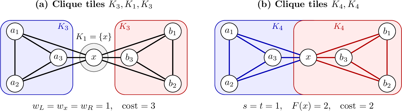
Figure 2 shows why both the tile family and its weights matter once the tiles interact. Let \(L=\{a_1,a_2,a_3\}\) and \(R=\{b_1,b_2,b_3\}\) be disjoint triangles, and let \(x\) be adjacent to all six side vertices, with no edges between \(L\) and \(R\). Then \(\alpha(G)=2\): one may choose one vertex from each side, whereas choosing \(x\) excludes every other vertex. In panel (a), assign weights \(w_L,w_x,w_R\) to the disjoint tiles \(L,\{x\},R\). The coverage constraints force \(w_L\geqslant 1\), \(w_x\geqslant 1\), and \(w_R\geqslant 1\), so every feasible choice has cost at least three. Unit weights attain this minimum and give \(F\equiv1\), but the resulting bound is not sharp. No different choice of weights can repair this tile family.
In panel (b), take instead the two overlapping tiles \(T_L=G[L\cup\{x\}]\) and \(T_R=G[R\cup\{x\}]\), both isomorphic to \(K_4\), with weights \(s\) and \(t\). Their coverages and cost are \[F(a_i)=s,\qquad F(b_j)=t,\qquad F(x)=s+t, \qquad \mathop{\mathrm{cost}}=s+t.\] Indeed, each \(a_i\) lies only in \(T_L\), each \(b_j\) lies only in \(T_R\), and \(x\) lies in both tiles. Covering the left and right side vertices therefore forces \(s\geqslant 1\) and \(t\geqslant 1\); covering \(x\) imposes only the weaker condition \(s+t\geqslant 1\). The minimum is attained at \(s=t=1\). At these weights every side vertex has coverage one and \(x\) has coverage two. Since each tile is a \(K_4\), it has independence number one, and the weighted local-cover bound gives \[\alpha(G)\leqslant 1\cdot\alpha(T_L)+1\cdot\alpha(T_R)=2.\] Conversely, any pair consisting of one vertex of \(L\) and one vertex of \(R\) is independent, because there are no edges between the two sides. Hence \(\alpha(G)=2\), and the bound from panel (b) is sharp. By contrast, \(s=t=1/2\) covers the central vertex exactly but leaves every side vertex with coverage \(1/2\), so it is not feasible. A successful certificate therefore requires both suitable tile shapes and suitable weights.
The disjoint situation in panel (a) is a useful baseline, but it is less representative of our applications. There the tiles are algebraically structured translates, often of coset-like sets, and different translates typically overlap; the relevant difficulty is therefore closer to panel (b). The algebraic structure lets us control the independence number of each tile and the pattern of its incidences, but it does not by itself make the resulting bound sharp. The main work of the paper is to choose structured tile families and weights for which these overlapping local bounds combine to give the desired exact global bound.
The dual of ?? is the fractional packing program \[\begin{align} \text{maximize}\quad&\sum_{x\in V}y_x,\\ \text{subject to}\quad&\sum_{x\in V(T)}y_x\leqslant\alpha(T) &&(T\in\mathcal{T}),\\ &y_x\geqslant 0&&(x\in V). \end{align} \label{eq:abstract-tile-dual}\tag{8}\] If all templates are cliques, this is the usual fractional clique-cover bound; see [6]. The applications here use translated non-clique templates with known independence numbers. This is distinct from the Delsarte linear program, whose variables are distance distributions in an association scheme [7].
A fractional local cover is exact if \(F(x)=1\) for every vertex. If all positive-weight templates have common density \[\mathop{\mathrm{dens}}(T)=\frac{\alpha(T)}{|V(T)|}=\rho,\] define the total overcoverage by \[E(F)=\sum_{x\in V}(F(x)-1).\] Double counting gives the defect identity \[\mathop{\mathrm{cost}}(\mathcal{T},w)=\rho\bigl(|V|+E(F)\bigr). \label{eq:abstract-defect}\tag{9}\] In particular, an exact cover has cost \(\rho|V|\). If \(G\) has a proper \(q\)-coloring, every induced subgraph has independence density at least \(1/q\). We call a template exact-density when \[\alpha(T)=\frac{|V(T)|}{q}. \label{eq:exact-density-general}\tag{10}\] Together with Theorem 2, a cover by exact-density templates therefore gives \[\alpha(G)\leqslant\frac{|V|+E(F)}{q}. \label{eq:exact-density-bound}\tag{11}\] Thus \(E(F)<q\) implies \(\alpha(G)\leqslant\lceil |V|/q\rceil\). More generally, if \(B\) is an integer lower target, a cover of cost strictly smaller than \(B+1\) proves \(\alpha(G)\leqslant B\).
We now isolate the finite-state step. Fix a finite family \[\mathcal{H}=\{U_j\subseteq\Delta_q(r_j):1\leqslant j\leqslant s\}.\] The translate with anchor \(a\in\Delta_q(d-r_j)\) has vertex set \(a+U_j\). Only translation invariance and the independence number of each tile are used. For a cap \(C\geqslant 0\), write \[\tau_C(a)=(\min(a_1,C),\ldots,\min(a_q,C)).\] We assign the translate \(a+U_j\) the weight \(z_{j,\tau_C(a)}\). The state is initially ordered; coordinate symmetry will later permit sorting. Fix also a starting degree \(d_0\), a modulus \(L\), a residue class \(\ell\pmod L\), a polynomial function \(P_\ell(d)\) of degree at most \(q-1\), and a constant \(\delta\). We seek nonnegative rational weights and one constant \(\delta'\leqslant\delta\) such that, for every \(d\geqslant d_0\) with \(d\equiv\ell\pmod L\), \[F_d(x)\geqslant 1\quad(x\in\Delta_q(d)), \qquad \mathop{\mathrm{cost}}(F_d)=P_\ell(d)+\delta'. \label{eq:finite-state-goal}\tag{12}\]
Theorem 4 (Finite-state reduction). For the data fixed above, the requirements in 12 are equivalent to the feasibility of a finite rational linear system.
Proof. For \(x\in\Delta_q(d)\), the coverage is \[F_d(x)=\sum_{j=1}^s\; \sum_{\substack{u\in U_j\\u\leqslant x}} z_{j,\tau_C(x-u)}, \label{eq:state-coverage-formula}\tag{13}\] where \(u\leqslant x\) is coordinatewise. Put \(R=\max_j r_j\), \(D=C+R\), and \[\sigma_D(x)=(\min(x_1,D),\ldots,\min(x_q,D)).\] Suppose that \(x_i\geqslant D\). Since \(0\leqslant u_i\leqslant r_j\leqslant R\), we have \(x_i-u_i\geqslant C\), and therefore the \(i\)th coordinate of \(\tau_C(x-u)\) is \(C\), independently of the actual value of \(x_i\). If \(x_i<D\), the state \(\sigma_D(x)\) records \(x_i\) exactly and hence also records whether \(u_i\leqslant x_i\) and the value of \(\min(x_i-u_i,C)\). Thus every summand and every eligibility condition in 13 is determined by \(j\), \(u\), and \(\sigma_D(x)\). There are only \((D+1)^q-D^q\) saturated ordered states, so all saturated coverage inequalities form a finite system. If \(x\) is unsaturated, then \(x_i\leqslant D-1\) for every \(i\), so \(d=|x|\leqslant q(D-1)\). Hence only finitely many unsaturated profiles remain.
For the cost, fix a state \(t\) with capped coordinate set \(K\), \(|K|=k\). The coordinates outside \(K\) are fixed by \(t\). For \(i\in K\), write \(a_i=C+y_i\) with \(y_i\geqslant 0\). The anchor equation \(|a|=d-r_j\) becomes \[\sum_{i\in K}y_i=d-r_j-|t|.\] For \(k\geqslant 1\), stars and bars gives \[m_{j,t}(d)= \binom{d-r_j-|t|+k-1}{k-1}, \label{eq:general-state-multiplicity}\tag{14}\] whenever the state is feasible; for \(k=0\), every coordinate is fixed. Multiplying these multiplicities by the fixed local costs \(\alpha(G_q(r_j)[U_j])\) and the weights \(z_{j,t}\) shows that the total cost is a polynomial in \(d\) of degree at most \(q-1\), with coefficients that are rational linear forms in the variables \(z_{j,t}\).
All coverage coefficients are integers, and the coefficients of the multiplicity polynomials are rational. Choose a threshold \(d_1\geqslant d_0\) after which every capped anchor state having a capped coordinate is feasible. For a fixed residue class, impose the finite saturated inequalities, the finitely many unsaturated inequalities, and nonnegativity. For \(d\geqslant d_1\), matching the coefficients of \(d^m\), \(m\geqslant 1\), between the cost and \(P_\ell(d)\) gives finitely many rational linear equations, and the constant coefficient is written as the additional variable \(\delta'\) with \(\delta'\leqslant\delta\). For each of the finitely many transition degrees \[d_0\leqslant d<d_1,\qquad d\equiv\ell\pmod L,\] include the directly evaluated coverage inequalities and the linear identity \(\mathop{\mathrm{cost}}(F_d)=P_\ell(d)+\delta'\). These finitely many constraints are exactly the finite rational system asserted in the statement. ◻
All families used below are invariant under permuting the \(q\) coordinates. Averaging the weights over these permutations preserves both coverage and cost. We may therefore assume that a weight depends only on the sorted capped anchor profile, and it is enough to impose one coverage inequality for each sorted capped vertex profile.
4 Three variables: planar local covers↩︎
The ternary case is the first exact application of Theorem 4. It gives a new proof of the Geramita–Gregory–Roberts formula and displays, in two dimensions, the same boundary-state mechanism used in the subsequent cases. Specializing the additive coloring above to \(A=\mathbb{Z}_3\) gives \[\alpha_3(d)\geqslant \left\lceil\frac{(d+1)(d+2)}{6}\right\rceil. \label{eq:q3-lower-frac}\tag{15}\] The degrees two and four are exceptional: their independence numbers are three and six, respectively.
For degrees divisible by three the extremal set has a particularly attractive geometric form. Figure 3 shows the degree-twelve example displayed by Machacek: the red vertices form the unique maximum independent set. Machacek’s argument proves uniqueness by forcing the boundary pattern and then moving inward [4]. We use the picture only as geometric motivation. The proof below is different: it bounds the size by a weighted cover of translated smaller simplices and does not use uniqueness.
![Figure 3: The unique maximum independent set of G_3(12), shown in red.It has 31 vertices and is the zero class ofa_2+2a_3\pmod 3; compare [4].](/article/2607.13733/_pdflatex/iyvczjum.png "fig:")
The residual degrees used in the eventual cover are \[\mathcal{R}_3=\{1,5,7,8\}. \label{eq:q3-residual-set}\tag{16}\] Exact finite computations give \[\begin{array}{c|rrrr} r&1&5&7&8\\ \hline |\Delta_3(r)|&3&21&36&45\\ \alpha_3(r)&1&7&12&15 \end{array}\] and hence \[\alpha_3(r)=\frac{|\Delta_3(r)|}{3} \qquad(r\in\mathcal{R}_3). \label{eq:q3-exact-density}\tag{17}\] Equation 17 is the reason for choosing these tiles. The additive coloring forces every tile to have independence density at least \(1/3\), and the weighted local-cover bound charges a tile of weight \(w\) the cost \(w\alpha(H)=w|V(H)|/3\). Hence an exact cover has total cost \(|\Delta_3(d)|/3\), while a cover whose total overcoverage is below three still gives the required integer upper bound through 18 . A tile of density greater than \(1/3\) would introduce a loss before the boundary is considered. Among the full simplices of residual degree at most eight, the four displayed degrees are exactly those of density \(1/3\); degrees two and four are genuine exceptions, and the remaining degrees fail the necessary divisibility condition. The finite-state system then shows that translates of these four shapes provide enough freedom near the boundary to keep the defect below three. The exact rational vector below certifies their sufficiency; no uniqueness or minimality is claimed.
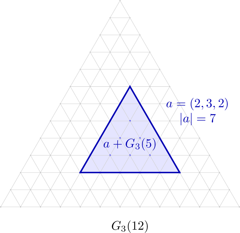
For \(a\in\Delta_3(d-r)\), the translate \[a+\Delta_3(r)\] induces a copy of \(G_3(r)\) inside \(G_3(d)\). Figure 4 shows a copy of \(G_3(5)\) inside \(G_3(12)\). The anchor fixes a common background exponent vector, while the residual degree-five mass moves inside the smaller triangle.
Assign weights \(w_{r,a}\geqslant 0\), and let \(\mathbf{1}_{r,a}(x)\) denote the indicator of the fixed-vertex statement \(x\in a+\Delta_3(r)\). Define \[F(x)=\sum_{r\in\mathcal{R}_3} \sum_{a\in\Delta_3(d-r)}w_{r,a}\mathbf{1}_{r,a}(x).\] If \(F(x)\geqslant 1\) for every vertex, then every independent set \(I\) satisfies \[|I|\leqslant\sum_{r,a}w_{r,a}\alpha_3(r).\] Using 17 and changing the order of summation gives \[\operatorname{cost}(F)-\frac{|\Delta_3(d)|}{3} =\frac{1}{3}\sum_{x\in\Delta_3(d)}(F(x)-1). \label{eq:q3-defect}\tag{18}\] Thus total overcoverage below three proves the sharp checksum upper bound.
Set the anchor cap to five and let \[\tau(a)=\operatorname{sort}(\min(a_1,5),\min(a_2,5),\min(a_3,5)).\] For \(d\geqslant 21\), every anchor associated with a residual degree at most eight has at least one capped coordinate. There are twenty-one anchor states and therefore \[4\cdot21=84\] variables \(z_{r,\tau}\). Capping vertex coordinates at \(5+8=13\) produces 105 saturated vertex states. The unsaturated profiles have all coordinates at most twelve; among them, only 167 have total degree at least twenty-one. The cost is a quadratic polynomial in \(d\), so the coefficients of \(d^2\) and \(d\) are matched exactly and the constant excess is minimized.
Proposition 5 (Ternary eventual certificate). There is a nonnegative rational state vector with forty-two positive coordinates such that all 105 saturated-state inequalities and all 167 relevant unsaturated inequalities hold, the two nonconstant cost coefficients match exactly, and \[\operatorname{cost}(F)-\frac{|\Delta_3(d)|}{3} =\delta_3=\frac{5}{7}<1 \qquad(d\geqslant 21).\] Consequently the total coverage defect is \(3\delta_3<3\).
The state vector, every state inequality, and every coefficient identity were verified by exact computer arithmetic. The finitely many degrees below twenty-one were checked in the same way by exact rational local covers; degrees two and four are the two direct exceptions. This proves the following formula by the same mechanism that will be used in five variables.
Theorem 6 (Exact ternary spreading number). For every \(d\geqslant 1\), \[\alpha_3(d)= \begin{cases} 3,&d=2,\\ 6,&d=4,\\ \displaystyle\left\lceil\frac{(d+1)(d+2)}{6}\right\rceil, &d\notin\{2,4\}. \end{cases}\]
Proof. The additive coloring gives the lower bound outside degrees two and four. Proposition 5 gives the matching upper bound for \(d\geqslant 21\), and the finite covers described above handle the remaining degrees. The two exceptional values follow from their direct constructions. ◻
5 Four variables: parity and boundary corrections↩︎
We next apply the local-tile viewpoint to four variables. This case has a feature that does not occur for \(q=3\) or \(q=5\): the exact answer depends on the parity of the degree. Odd degrees admit an integral tiling by \(K_4\)’s, while even degrees are handled by a finite-state fractional cover using only the two full simplices \(G_4(1)\) and \(G_4(3)\). These are not two unrelated techniques: the odd construction is precisely the exact \(F\equiv1\) specialization of the same LP framework, whereas the even case requires nontrivial state-dependent weights. For \(k\geqslant 0\), write \[M_4(2k+1)=\frac{(k+1)(k+2)(2k+3)}{6}\] and \[M_4(2k)=\binom{k+3}{3}+\binom{k+1}{3} =\frac{(k+1)^3+2(k+1)}{3}.\] Equivalently, for even \(d\), \[M_4(d)=\frac{d^3}{24}+\frac{d^2}{4}+\frac{5d}{6}+1. \label{eq:q4-even-polynomial}\tag{19}\]
Label the four coordinates by the elements of \(H=\mathbb{F}_2^2\), and define \[\chi_4(a)=\sum_{h\in H}a_h\,h, \qquad a=(a_h)_{h\in H}\in\Delta_4(d).\] A unit transfer changes the color by a nonzero element of \(H\), so every fiber of \(\chi_4\) is independent.
If \(d=2k\), the zero fiber consists precisely of the vectors whose four coordinates are all even or all odd. Hence \[|\chi_4^{-1}(0)| =\binom{k+3}{3}+\binom{k+1}{3} =M_4(2k). \label{eq:q4-even-lower}\tag{20}\] For odd degree the four fibers have equal size, and therefore each has size \[\frac{1}{4}|\Delta_4(d)|=M_4(d).\]
5.1 Odd degree: an integral local tiling↩︎
Let \(d\) be odd and let \(C_0=\chi_4^{-1}(0)\). The parity pattern of a vertex in \(C_0\) is either \[(1,0,0,0) \qquad\text{or}\qquad (0,1,1,1),\] where the first coordinate is indexed by \(0\in H\).
For a center \(c\in C_0\) of the first type, define \[Q(c)=\{c-e_0+e_h:h\in H\}.\] For a center of the second type, define \[Q(c)=\{c+e_0-e_h:h\in H\}.\] The two orientations are dictated by parity rather than selected by a linear program. In the first parity orbit the distinguished \(0\)-coordinate is the unique odd coordinate, so one moves a unit out of that coordinate; in the second it is the unique even coordinate, so the move is reversed. Every vector of odd coordinate sum has either one or three odd coordinates. Its parity pattern therefore determines the orientation and the transferred coordinate, after which the vector itself determines the unique zero-color center. Thus the two parity orbits force exactly the two orientations needed for the partition. Each \(Q(c)\) is a \(K_4\), and the resulting vertex sets form the disjoint union \[\Delta_4(d)=\bigsqcup_{c\in C_0}Q(c). \label{eq:q4-odd-tiling}\tag{21}\] Every independent set meets each tile in at most one vertex, whereas \(C_0\) meets every tile exactly once. Therefore \[\alpha_4(d)=\frac{1}{4}\binom{d+3}{3}=M_4(d) \qquad(d\text{ odd}). \label{eq:q4-odd-value}\tag{22}\] This is an integral local-tile certificate. It uses the two orientations of a degree-one simplex: the first family consists of ordinary translates of \(G_4(1)\), while the second is the reflected orientation. In the language of the preceding terminology, all selected weights are one and \(F\equiv1\). Thus the associated linear program is solved by inspection: it is the zero-defect case of the general framework.
5.2 Even degree: exact-density templates↩︎
For even degree we use ordinary translated full simplices only. Set \[\mathcal{R}_4=\{1,3\}. \label{eq:q4-residual-set}\tag{23}\] The two local capacities are \[\begin{array}{c|cc} r&1&3\\ \hline |\Delta_4(r)|&4&20\\ \alpha_4(r)&1&5 \end{array}\] and hence \[\alpha_4(r)=\frac{|\Delta_4(r)|}{4} \qquad(r\in\mathcal{R}_4). \label{eq:q4-exact-density}\tag{24}\]
Here again the density condition is the first filter. The degree-one tile is the smallest local \(K_4\), while degree three is the smallest thicker full simplex with the same optimal density. Together, these two scales give the state weights enough freedom near faces and lower-dimensional strata to reproduce the unavoidable linear boundary excess in 26 . The rational certificate below proves that they suffice. Their sufficiency was found by the finite-state search; no uniqueness or minimality of \(\{1,3\}\) is asserted.
Assign a nonnegative weight \(w_{r,a}\) to every translate \(a+\Delta_4(r)\), and let \(\mathbf{1}_{r,a}(x)\) be the indicator of \(x\in a+\Delta_4(r)\). Then \[F(x)= \sum_{r\in\mathcal{R}_4} \sum_{a\in\Delta_4(d-r)}w_{r,a}\mathbf{1}_{r,a}(x).\] If \(F(x)\geqslant 1\) for every vertex, then every independent set satisfies \[|I|\leqslant\operatorname{cost}(F) :=\sum_{r,a}w_{r,a}\alpha_4(r).\] As before, exact local density gives the defect identity \[\operatorname{cost}(F)-\frac{1}{4}|\Delta_4(d)| =\frac{1}{4}\sum_{x\in\Delta_4(d)}(F(x)-1). \label{eq:q4-defect}\tag{25}\] Unlike the odd case, the optimal even value is larger than the average by a linear boundary term: \[M_4(d)-\frac{1}{4}|\Delta_4(d)| =\frac{3d}{8}+\frac{3}{4} \qquad(d\text{ even}). \label{eq:q4-boundary-excess}\tag{26}\] Thus the purpose of the linear program is not to make the defect bounded, but to reproduce this exact boundary slack.
Set the anchor cap to \(C=3\) and define \[\tau(a)=\operatorname{sort} \bigl(\min(a_1,3),\ldots,\min(a_4,3)\bigr).\] There are \[\binom{6}{3}=20\] anchor states, and hence \(2\cdot20=40\) variables \(z_{r,\tau}\). Capping vertex coordinates at \(C+\max\mathcal{R}_4=6\) gives \(84\) saturated states. The certificate also checks the \(18\) unsaturated sorted profiles with entries at most five and total at least fifteen. The anchor-state multiplicities are polynomials of degree at most three in \(d\). We match the coefficients of \(d^3,d^2,d\) to those in 19 and minimize the constant coefficient.
Proposition 7 (Exact quaternary even-degree certificate). There is a nonnegative rational state vector with twenty-nine positive coordinates such that all \(84+18\) state inequalities hold and \[\operatorname{cost}(F) =\frac{d^3}{24}+\frac{d^2}{4}+\frac{5d}{6}+1 \label{eq:q4-even-exact-cost}\qquad{(2)}\] for every \(d\geqslant 15\). For every even \(d\geqslant 16\), this polynomial is exactly \(M_4(d)\), and hence gives the sharp upper bound.
The vector uses only the residual degrees \(1\) and \(3\), anchor cap three, forty state variables, and twenty-nine positive coordinates. Its minimum state coverage is exactly one. All state inequalities, coefficient identities, and direct reconstructions of the relevant tetrahedra were verified by exact computer arithmetic. For the remaining even degrees \[d=2,4,6,8,10,12,14,\] exact rational local-cover certificates using the same two residual degrees have costs \[4,11,24,45,76,119,176,\] respectively. These are exactly the values \(M_4(d)\). The covers and their costs were verified by exact computer arithmetic.
Theorem 8 (Exact quaternary spreading number). For every \(k\geqslant 0\), \[\alpha_4(2k+1) =\frac{(k+1)(k+2)(2k+3)}{6},\] and \[\alpha_4(2k) =\binom{k+3}{3}+\binom{k+1}{3}.\]
Proof. The additive coloring gives the lower bounds. For odd degree, the integral \(K_4\)-tiling 21 gives the matching upper bound. For even \(d\geqslant 16\), Proposition 7 gives \(|I|\leqslant M_4(d)\). The seven exact finite covers give the same bound for the remaining positive even degrees. For \(d=0\), the graph has one vertex, in agreement with the displayed formula. Hence the additive constructions are optimal in every degree. ◻
Remark 9. The parity split is intrinsic. In odd degree the optimum equals the average color-class size and is witnessed by an exact integral tiling using both orientations of \(G_4(1)\). In even degree the optimum exceeds the average by \(3d/8+3/4\); the fractional \(\{1,3\}\)-tile cover reproduces precisely this boundary contribution.
6 The case \(q=5\): exact local tiles↩︎
The cyclic coloring gives \[\alpha_5(d)\geqslant \left\lceil\frac{1}{5}\binom{d+4}{4}\right\rceil. \label{eq:q5-lower}\tag{27}\] There are two exceptions to equality. The sets \[\{2e_i:i\in[5]\}\] and \[\{4e_i:i\in[5]\} \;\cup\;\{2e_i+2e_j:1\leqslant i<j\leqslant 5\} \;\cup\;\{(0,1,1,1,1)\} \label{eq:q5-d4-exception}\tag{28}\] are independent and have sizes \(5\) and \(16\), respectively. We prove that these are the only exceptions.
The eventual argument uses only translated smaller copies of the same graph. Set \[\mathcal{R}_5=\{1,3,6,7,8,9\}. \label{eq:q5-residual-set}\tag{29}\] For these residual degrees the exact finite values are \[\begin{array}{c|rrrrrr} r&1&3&6&7&8&9\\ \hline |\Delta_5(r)|&5&35&210&330&495&715\\ \alpha_5(r)&1&7&42&66&99&143. \end{array}\] Thus \[\alpha_5(r)=\frac{|\Delta_5(r)|}{5} \qquad(r\in\mathcal{R}_5). \label{eq:q5-exact-density}\tag{30}\] These are precisely the exact-density full simplices of residual degree at most nine. The choice is therefore intrinsic: every tile is a genuine smaller discrete simplex, it retains full coordinate symmetry, and it pays no local density penalty.
For \(a\in\Delta_5(d-r)\), the translate \[a+\Delta_5(r)\] induces a copy of \(G_5(r)\) inside \(G_5(d)\). Hence every independent set \(I\) satisfies \[|I\cap(a+\Delta_5(r))|\leqslant\alpha_5(r).\] By 30 and the defect identity 9 , any fractional cover by these tiles with total overcoverage below five proves the upper bound in 27 .
We now construct one finite-state cover valid for every \(d\geqslant 35\). Give the translate \(a+\Delta_5(r)\) a weight depending only on \(r\) and on \[\tau(a)=\operatorname{sort}\bigl(\min(a_1,6),\ldots,\min(a_5,6)\bigr).\] There are \(210\) sorted anchor states and six residual degrees, hence \(1260\) variables. Since the largest residual degree is nine, coverage is determined by the finitely many sorted vertex profiles obtained by capping coordinates at fifteen, together with the unsaturated profiles of total degree at least thirty-five. If an anchor state \(\tau\) has \(k\) capped entries and the residual degree is \(r\), and \(\operatorname{Orb}(\tau)\) denotes its set of distinct coordinate permutations, its multiplicity in degree \(d\) is \[m_{r,\tau}(d)=|\operatorname{Orb}(\tau)| \binom{d-r-|\tau|+k-1}{k-1}, \label{eq:q5-state-multiplicity}\tag{31}\] with the usual value zero when infeasible. Consequently the cost of a fixed state vector is a polynomial function of \(d\) of degree at most four.
Proposition 10 (Exact eventual certificate). There is a nonnegative rational state vector with \(933\) positive coordinates among the \(1260\) variables which covers every vertex for every \(d\geqslant 35\) and satisfies \[\mathop{\mathrm{cost}}(F_d)-\frac{1}{5}\binom{d+4}{4}=\delta_5<1.\] Consequently \[\alpha_5(d)=\left\lceil\frac{1}{5}\binom{d+4}{4}\right\rceil \qquad(d\geqslant 35).\]
This is a finite rational system: its \(1260\) variables, all capped and uncapped coverage inequalities, and the four coefficient identities for the cost function were checked by exact computer arithmetic. It remains to treat the finite range \(1\leqslant d\leqslant 34\).
Proposition 11 (Finite computation). The exact values for \(1\leqslant d\leqslant 34\) are those asserted in Theorem 12 below.
For \(d\leqslant 9\) this is a finite maximum-independent-set calculation; degree five also has the direct proof in Proposition 23. For \(10\leqslant d\leqslant 34\) the result follows from exact rational local covers of cost below the claimed integer bound plus one. These are finite systems, and all coverage inequalities and objective values were checked exactly by computer.
Theorem 12 (Exact five-variable spreading number). For every \(d\geqslant 1\), \[\alpha_5(d)= \begin{cases} 5,&d=2,\\ 16,&d=4,\\ \displaystyle\left\lceil\frac{1}{5}\binom{d+4}{4}\right\rceil, &d\notin\{2,4\}. \end{cases}\]
Proof. The additive coloring and the two displayed exceptional sets give the lower bounds. Proposition 11 covers \(1\leqslant d\leqslant 34\), and Proposition 10 covers every \(d\geqslant 35\). ◻
7 The case \(q=7\): the complete solution↩︎
The cyclic checksum fibers give the lower bound \[L_7(d):=\left\lceil\frac{1}{7}\binom{d+6}{6}\right\rceil.\] Every vector used in this section still has seven coordinates. Let \(e_1,\ldots,e_7\) be the standard unit vectors of \(\mathbb{Z}^7\). If \(\lambda=(\lambda_1,\ldots,\lambda_k)\) is a partition of \(r\) with \(k\leqslant 7\), set \[\mathcal{O}_7(\lambda) =\{\text{coordinate permutations of } (\lambda_1,\ldots,\lambda_k,0,\ldots,0)\}.\] Equivalently, deleting the zero coordinates of \(u\in\mathcal{O}_7(\lambda)\) and arranging the remaining values in decreasing order gives \(\lambda\). This ordering records the values only; it imposes no order on their coordinate indices. For example, \[\mathcal{O}_7(2,1)=\{2e_i+e_j:i,j\in[7],\;i\ne j\}, \qquad \mathcal{O}_7(2,2)=\{2e_i+2e_j:i<j\}.\] The first set has \(7\cdot6=42\) elements: exchanging \(i\) and \(j\) moves the entries \(2\) and \(1\) and therefore gives a different vector. The abbreviation \((1^k)\) means \(k\) parts equal to one.
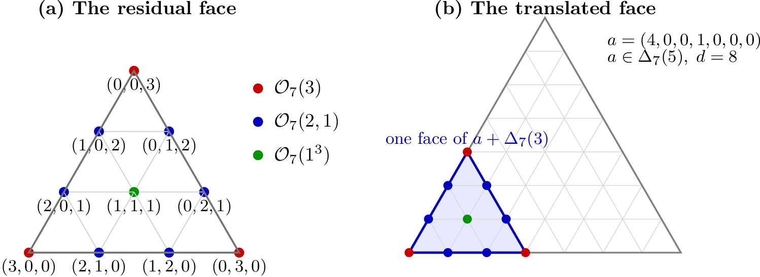
In the three- and five-variable proofs, translated full residual simplices provided enough local information. For seven variables they do not distinguish the boundary layers finely enough to obtain the sharp bound in all degrees. We therefore decompose each small simplex \(\Delta_7(r)\) into its coordinate-permutation orbits \(\mathcal{O}_7(\lambda)\) and build a tile by taking a union of selected orbits. This preserves the full symmetry among the seven coordinates while allowing different boundary profiles to be covered separately. Figure 5 shows the three orbits that occur in residual degree three and then shows how the same local pattern is moved by an anchor. In general, for a fixed anchor \(a\) and an orbit union \(U\subseteq\Delta_7(r)\), the whole placement satisfies \(a+U\subseteq a+\Delta_7(r)\subseteq\Delta_7(d)\); varying \(a\) moves this small copy through the ambient simplex. The orbit unions defined immediately afterward are the extra flexibility that makes the complete seven-variable cover possible.
We now define the tiles before summarizing them. Let \[\begin{align} U_1&=\mathcal{O}_7(1),& U_2&=\mathcal{O}_7(1^2),& U_3&=\mathcal{O}_7(1^3),\\ U_4&=\mathcal{O}_7(2,1)\cup\mathcal{O}_7(1^3),& U_5&=\mathcal{O}_7(1^4),& U_6&=\mathcal{O}_7(3,1)\cup\mathcal{O}_7(2,1,1) \cup\mathcal{O}_7(1^4),\\ U_7&=\mathcal{O}_7(1^5),& U_8&=\mathcal{O}_7(1^6),& U_9&=\mathcal{O}_7(3)\cup\mathcal{O}_7(2,1),\\ U_{10}&=\mathcal{O}_7(4)\cup\mathcal{O}_7(3,1),& U_{11}&=\mathcal{O}_7(3,1)\cup\mathcal{O}_7(2,1,1),& U_{12}&=\mathcal{O}_7(3,1)\cup\mathcal{O}_7(2,2) \cup\mathcal{O}_7(2,1,1),\\ U_{13}&=\Delta_7(5).&&& \end{align}\] Their residual degrees are \[(r_1,\ldots,r_{13})=(1,2,3,3,4,4,5,6,3,4,4,4,5),\] and the corresponding base tiles are \[H_t=G_7(r_t)[U_t], \qquad \mathcal{H}_7=\{H_1,\ldots,H_{13}\}.\] This is the same construction used in the preceding sections. For each \(t\) and each anchor \(a\in\Delta_7(d-r_t)\), the placed tile has vertex set \(a+U_t\), and the full family of placements is \[\mathcal{T}_7(d)= \{a+H_t:1\leqslant t\leqslant 13,\;a\in\Delta_7(d-r_t)\}. \label{eq:q7-placed-family}\tag{32}\] Both \(a\) and every \(u\in U_t\) have length seven; only their total masses are \(d-r_t\) and \(r_t\). Orbit notation records the pattern of the residual vector \(u\) and does not shorten the anchor or change the ambient dimension. The symbol \(a\) is local to a placement: different tile degrees have their own anchor sets, and every admissible anchor is used. We later assign a weight \(w_{t,a}\) to each placement and group equal weights only after capping and sorting the seven coordinates of \(a\).
For a concrete example, \(U_4\) is the union of the \(42\) vectors of type \((2,1)\) and the \(\binom73=35\) vectors of type \((1^3)\), so \(H_4\) has \(77\) vertices. The more elaborate degree-four set is \[\begin{align} U_{12} ={}&\{3e_i+e_j:i\ne j\} \cup\{2e_i+2e_j:i<j\}\\ &\cup\{2e_i+e_j+e_k:i,j,k\text{ distinct},\;j<k\}. \end{align}\] Its three parts have \(42\), \(21\), and \(105\) vertices. A placement of this tile is \(a+U_{12}\) with \(a\in\Delta_7(d-4)\): the same seven-coordinate background vector \(a\) is added to every residual vector displayed above.
The first natural choice consists of \(H_1,\ldots,H_8\). These tiles already give an exact finite-state cover for every \(d\geqslant 30\), but its cost is \[\frac{1}{7}\binom{d+6}{6}+\frac{43}{42}. \label{eq:q7-simple-cost}\tag{33}\] Here the anchor cap is four: the finite system has \(1680\) variables and \(1716\) saturated profile inequalities, together with the finite unsaturated range \(30\leqslant d\leqslant 42\). When \(7\mid d\), integrality turns this into the desired bound; thus these tiles alone prove the formula for all multiples of seven from \(d=35\) onward (and for even multiples from \(d=42\) onward). If \(7\nmid d\), however, the excess \(43/42>1\) leaves an entire integer unaccounted for. The simple family therefore captures a genuine infinite subfamily, but not the full theorem. To correct the remaining boundary profiles we add \(H_9,\ldots,H_{13}\). They were chosen for two simultaneous reasons: each has independence density \(1/7\), so it introduces no bulk loss, and together they meet the profile layers that are under-covered in 33 . The following table merely collects the definitions and the local independence numbers.
| tile | degree \(r\) | profile types in \(U\) | \(|U|\) | \(\alpha(G_7(r)[U])\) |
|---|---|---|---|---|
| \(H_1\) | 1 | \((1)\) | 7 | 1 |
| \(H_2\) | 2 | \((1^2)\) | 21 | 3 |
| \(H_3\) | 3 | \((1^3)\) | 35 | 7 |
| \(H_4\) | 3 | \((2,1)\cup(1^3)\) | 77 | 11 |
| \(H_5\) | 4 | \((1^4)\) | 35 | 7 |
| \(H_6\) | 4 | \((3,1)\cup(2,1,1)\cup(1^4)\) | 182 | 26 |
| \(H_7\) | 5 | \((1^5)\) | 21 | 3 |
| \(H_8\) | 6 | \((1^6)\) | 7 | 1 |
| \(H_9\) | 3 | \((3)\cup(2,1)\) | 49 | 7 |
| \(H_{10}\) | 4 | \((4)\cup(3,1)\) | 49 | 7 |
| \(H_{11}\) | 4 | \((3,1)\cup(2,1,1)\) | 147 | 21 |
| \(H_{12}\) | 4 | \((3,1)\cup(2,2)\cup(2,1,1)\) | 168 | 24 |
| \(H_{13}\) | 5 | all profiles in \(\Delta_7(5)\) | 462 | 66 |
The five corrections also have a direct geometric meaning. The tile \(H_9\) joins the corner layer \((3)\) to its first inward layer \((2,1)\) and is the disjoint union of seven upward \(K_7\)’s; \(H_{10}\) is the analogous correction in residual degree four. The tiles \(H_{11}\) and \(H_{12}\) join the degree-four layers concentrated on two or three coordinates, while \(H_{13}=G_7(5)\) is a full residual simplex and supplies a thicker interior scale. Thus the larger family adds exact-density shapes at precisely the corner, edge, and interior boundary scales missed by \(H_1,\ldots,H_8\). The eventual construction is one weighted cover formed from all placements in 32 , not thirteen separate decompositions of \(G_7(d)\).
This example also shows why the method does not immediately settle every prime \(q\). As \(q\) grows, more boundary profile types appear and the tiles needed to cover them become less simple. The finite system also grows quickly: with \(s\) tile types and anchor cap \(C\), the saturated anchor states alone give \[s\binom{C+q-1}{q-1}\] weight variables. Thus the reduction remains finite, but finding a useful family and solving the resulting system become harder. We nevertheless expect Conjecture 1 to hold for every prime \(q\): the checksum formula should be correct for all sufficiently large \(d\), while finitely many small degrees may remain exceptional, as they do for \(q=3,5,7\).
Lemma 1 (Local capacities). The thirteen independence numbers in Table 2 are exact.
Proof. The squarefree layers \(H_1,H_2,H_3,H_5,H_7,H_8\) give the clique, matching, pair-packing, and complementary pair-packing bounds; the Fano lines attain the values for \(H_3\) and \(H_5\). For \(H_4\), if an independent collection contains \(s\) triples, their \(3s\) pairs are unavailable to the directed type-\((2,1)\) vertices. The two ranges \(s\leqslant 4\) and \(s\geqslant 5\) both give a total at most \(11\). In \(H_6\), the type-\((2,1,1)\) vertices with a fixed doubled coordinate form a matching of size at most three, reduced to two when a type-\((3,1)\) vertex is present; the type-\((1^4)\) layer then gives the bound \(26\).
The tiles \(H_9\) and \(H_{10}\) split into seven heavy-coordinate cliques, and the same matching argument gives \(\alpha(H_{11})=21\). For \(H_{12}\), regard the selected type-\((2,2)\) vertices as the edges of a graph \(K\) on seven coordinates, with degrees \(d_i\). The remaining contribution at coordinate \(i\) is at most \(3-\lfloor d_i/2\rfloor\), whence \[|I|\leqslant|E(K)|+21-\sum_i\left\lfloor\frac{d_i}{2}\right\rfloor =21+\frac{\#\{i:d_i\text{ odd}\}}{2}\leqslant 24.\] Cyclic fibers attain these bounds. Finally, \(H_{13}=G_7(5)\) has independence number \(66\), as determined by a finite exhaustive calculation. ◻
Cap every anchor coordinate at three and let a tile weight depend only on its type and its sorted capped anchor profile. There are \(84\) anchor profiles and hence \(13\cdot84=1092\) variables. Vertex coordinates may be capped at eight, leaving \(3003\) saturated vertex states.
Proposition 13 (Exact eventual certificate). There is a nonnegative rational state vector, supported on \(435\) variables, which covers \(G_7(d)\) for every \(d\geqslant 26\) and has cost \[\frac{1}{7}\binom{d+6}{6}+\delta_7, \qquad 0<\delta_7<1. \label{eq:q7-eventual-cost}\qquad{(3)}\]
The state vector, its cost identity, all \(3003\) saturated inequalities, and the \(1547\) unsaturated profiles needed for \(26\leqslant d\leqslant 49\) were verified by exact computer arithmetic. From degree \(50\) onward a coordinate is at least eight, so the saturated verification applies.
Proposition 14 (Exact transition range). The equality \(\alpha_7(d)=L_7(d)\) holds for every \(7\leqslant d\leqslant 25\).
For each \(7\leqslant d\leqslant 25\), a finite rational system gives a local cover of cost strictly below \(L_7(d)+1\). All inequalities and costs were checked exactly by computer, and integrality completes the argument. The one degree not covered by the eventual formula requires a separate finite calculation.
Proposition 15 (The exceptional degree). \[\alpha_7(6)=133. \label{eq:q7-d6}\qquad{(4)}\]
Proof. Label the coordinates by the seven nonzero vectors of \(\mathbb{F}_2^3\) and take the zero-syndrome fiber. A unit transfer changes its syndrome by the sum of two distinct labels, so the fiber is independent. Character averaging gives its size as \[\frac{1}{8}\left[\binom{12}{6}+7\binom63\right]=133.\]
For the upper bound, exact local inequalities first reduce a hypothetical independent set of size \(134\) to fifteen finite symmetry classes. Each class is a system on at most \(185\) binary profile variables, consisting only of adjacency and local-capacity constraints. Exact computer calculation shows that all fifteen systems are infeasible. Hence no \(134\)-set exists. ◻
Theorem 16 (Seven-variable spreading numbers). For every \(d\geqslant 1\), \[\alpha_7(d)= \begin{cases} 7,&d=2,\\ 14,&d=3,\\ 35,&d=4,\\ 133,&d=6,\\ \displaystyle\left\lceil\frac{1}{7}\binom{d+6}{6}\right\rceil, &d\notin\{2,3,4,6\}. \end{cases} \label{eq:q7-main}\qquad{(5)}\] In particular, the prime-checksum formula holds for every \(d\geqslant 7\), and the threshold seven is sharp.
Proof. Theorem 20 gives \(d\leqslant 4\), and Lemma 1 gives the finite base case \(d=5\). Proposition 15 handles degree six, while Proposition 14 handles \(7\leqslant d\leqslant 25\). For \(d\geqslant 26\), Proposition 13 gives the upper cover and the cyclic fiber gives the lower bound. If \(7\nmid d\), then \(\binom{d+6}{6}\) is divisible by seven and ?? has the same integer part as \(L_7(d)\). If \(7\mid d\), write \(\binom{d+6}{6}=7m+1\); the cover cost is strictly below \(m+2\). Integrality gives \(\alpha_7(d)\leqslant L_7(d)\) in both cases. ◻
Remark 17 (The nonuniform small-degree regime). The eventual checksum phenomenon should not be expected to be uniform in the alphabet size. When \(d<q\), a large proportion of the simplex lies near its boundary, and constructions arising from label groups other than \(\mathbb{Z}_q\) can outperform the cyclic checksum fiber. This already occurs at the exceptional degrees \(2\) and \(4\) for \(q=5\). For \(q=7\), the exact small-degree values at \(d=2,3,4\) also exceed the checksum value, and the nonzero \(\mathbb{F}_2^3\) labeling gives an independent set of size \(133\) at \(d=6\), whereas the cyclic checksum fiber has size \(132\). These examples suggest that further sporadic gaps may occur in the regime \(d<q\), even when the prime-checksum conjecture is eventually true for each fixed prime \(q\). The fixed-degree orbit reduction in Section 9 is designed to study precisely this complementary regime.
8 Additive targets and the scope of the method↩︎
The finite-state theorem is independent of the lower construction, but a sharp application needs a target polynomial or quasi-polynomial. Additive colorings provide such targets and explain the residue classes that appear in the local programs. We record two forms that will also be used in the fixed-degree comparison.
8.1 Balance of the cyclic checksum↩︎
The construction \(\mathcal{C}_{q,d}(r)\) from 4 provides an explicit independent set. Its exact class sizes are given in [5]. Put \[B_q(d)=\frac{1}{q}\binom{d+q-1}{q-1} =\frac{1}{q}|\Delta_q(d)|. \label{eq:checksum-average}\tag{34}\] For \(m\geqslant 1\), let \[c_m(r)=\sum_{\substack{1\leqslant k\leqslant m\\(k,m)=1}} \exp\!\left(\frac{2\pi\mathrm i kr}{m}\right)\] be the Ramanujan sum. Then \[N_r^{(q)}(d) =\frac{1}{q}\sum_{m\mid\gcd(q,d)} c_m(r)\binom{d/m+q/m-1}{q/m-1}. \label{eq:exact-checksum-balance}\tag{35}\] In particular, if \(q\) is prime, \[N_r^{(q)}(d)= \begin{cases} \displaystyle\frac{1}{q}\binom{d+q-1}{q-1}, &q\nmid d,\\[7pt] \displaystyle\frac{1}{q}\left[\binom{d+q-1}{q-1}+q-1\right], &q\mid d,\;r=0,\\[7pt] \displaystyle\frac{1}{q}\left[\binom{d+q-1}{q-1}-1\right], &q\mid d,\;r\ne0. \end{cases} \label{eq:prime-checksum-balance}\tag{36}\] Consequently, \[\max_{r\in\mathbb{Z}_q}N_r^{(q)}(d)=\left\lceil B_q(d)\right\rceil \qquad(q\text{ prime}). \label{eq:prime-checksum-maximum}\tag{37}\] If \(p_0\) is the smallest prime divisor of \(q\), then \[N_r^{(q)}(d)=B_q(d)+O_q\!\left(d^{q/p_0-1}\right) \qquad(d\to\infty). \label{eq:checksum-asymptotic-balance}\tag{38}\] The checksum construction and the one-deletion upper bound of Kovačević and Tan [8] give \[\max_{r\in\mathbb{Z}_q}N_r^{(q)}(d) \leqslant\alpha_q(d) \leqslant\frac{1}{q}\binom{d+q}{q-1} =B_q(d)+\frac{1}{q}\binom{d+q-1}{q-2}. \label{eq:checksum-KT-sandwich}\tag{39}\] The left side describes a concrete independent set; the right side bounds all independent sets.
8.2 Other additive label groups↩︎
The label group changes the lower-order terms of the target when \(q\) is composite. Write \[q=\prod_{p\mid q}q_p,\qquad q_p=p^{e_p}, \qquad A_q=\bigoplus_{p\mid q}\mathbb{F}_p^{e_p}.\] For \(S\subseteq\{p:p\mid q\}\), put \[m_S=\prod_{p\in S}p, \qquad \gamma_S=\prod_{p\in S}(q_p-1),\] with \(m_\varnothing=\gamma_\varnothing=1\).
Proposition 18 (Largest additive fiber). For the coloring of \(\Delta_q(d)\) by \(A_q\), the zero fiber has cardinality \[M_q(d)=\frac{1}{q} \sum_{\substack{S\subseteq\{p:p\mid q\}\\m_S\mid d}} \gamma_S \binom{d/m_S+q/m_S-1}{q/m_S-1}. \label{eq:general-zero-fiber}\qquad{(6)}\] It is a largest color class. In particular, \(\alpha_q(d)\geqslant M_q(d)\).
Proof. Apply the character filter to the generating function of nonnegative multiplicity vectors. A character whose nontrivial Sylow components are indexed by \(S\) has order \(m_S\), and \[\prod_{a\in A_q}(1-z\psi(a))^{-1} =(1-z^{m_S})^{-q/m_S}.\] There are \(\gamma_S\) such characters. Extracting the coefficient of \(z^d\) gives ?? . In the zero fiber all character contributions have positive sign, and the triangle inequality shows that no other fiber is larger. ◻
Proposition 18 has only two regimes when \(q=p^m\) is a prime power: \[M_q(d)= \begin{cases} \displaystyle\frac{1}{q}\binom{d+q-1}{q-1},&p\nmid d,\\[8pt] \displaystyle\frac{1}{q}\left[ \binom{d+q-1}{q-1}+(q-1) \binom{d/p+q/p-1}{q/p-1}\right],&p\mid d. \end{cases} \label{eq:prime-power-target}\tag{40}\] For \(q=4\), these are exactly the odd- and even-degree targets in Section 5. In general, \[M_q(d)=\frac{1}{q}\binom{d+q-1}{q-1} +O_q\bigl(d^{q/p_0-1}\bigr). \label{eq:general-target-asymptotic}\tag{41}\]
Four exact-density tile families occur in the fixed-alphabet applications. The ternary proof uses full simplices of residual degrees \(1,5,7,8\); the quaternary proof uses two oriented cliques in odd degree and full simplices of degrees \(1,3\) in even degree; the five-variable proof uses the full simplices of residual degrees in 29 ; and the seven-variable proof uses the mixed orbit-union templates in Section 7. The examples suggest that the main remaining difficulty is not state finiteness, which follows from Theorem 4, but template selection.
Conjecture 19 (Finite exact-density tile families). For every fixed \(q\), there is a finite coordinate-symmetric family of induced templates of independence density \(1/q\) such that, in every divisibility regime of ?? , the associated finite-state program certifies \[\alpha_q(d)=M_q(d)\] for all sufficiently large \(d\), apart from finitely many exceptional degrees.
The conjecture permits shapes other than full simplices. The four-variable odd-degree proof needs a reflected orientation, while the seven-variable proof uses the mixed orbit-union templates \(H_4\) and \(H_6\). Thus mixed tile families are not merely experimental: they are already essential in a sharp higher-dimensional application.
9 Orbit reductions at fixed degree↩︎
The previous section keeps \(q\) fixed and lets the ambient degree grow. A second reduction is available in the opposite direction: fix the degree \(d\) and exploit the full permutation symmetry of the \(q\) coordinates. In coding language, independent sets in \(G_q(d)\) are constant \(\ell_1\)-weight \(d\) codes of minimum \(\ell_1\)-distance four. The exact values for weights at most four were determined by Chen, Ma, and Zhang [9]. We first recover those values as explicit weighted-tiling certificates, then solve the degree-five orbit program and obtain exact power-of-two families in degrees six, eight, and ten. We finally derive a three-term fixed-degree asymptotic expansion, together with a conjectural hierarchy extending it. Thus the numerical results in Theorem 20 are known; the exact power-of-two families and the subsequent symbolic LP consequences are new applications of the weighted-tiling formalism.
The two tile families used in this section arise naturally from the deletion geometry. An anchor \(a\in\Delta_q(d-1)\) is a possible one-deletion output, and \(a+\Delta_q(1)\) is the set of all \(q\) words obtained by reinserting one symbol. These words are pairwise confusable, so they form a \(K_q\) and give the canonical inequality \(|I\cap(a+\Delta_q(1))|\leqslant 1\). Each such clique has density \(1/q\), matching the additive lower construction. Moreover, a vertex \(x\) lies precisely in the cliques anchored at \(x-e_i\) for its positive coordinates, so the coverage equations are predecessor equations and coordinate symmetry groups them by integer partitions. On the squarefree layer, supports are \(k\)-subsets and a unit transfer is a one-element exchange; the induced graph is therefore the Johnson graph \(J(q,k)\), whose independence number is the corresponding packing number.
For integers \(v\geqslant k\geqslant t\), let \(D(v,k,t)\) be the maximum number of \(k\)-subsets of a \(v\)-set such that no \(t\)-subset is contained in more than one block, and set \(D(v,k,t)=0\) when \(v<k\). Equivalently, with the empty Johnson layer understood when \(v<k\), \[D(v,k,k-1)=\alpha(J(v,k)),\] where \(J(v,k)\) is the Johnson graph in which two \(k\)-subsets are adjacent when they meet in \(k-1\) points.
Theorem 20 (The exact values in degrees two, three, and four). For every \(q\geqslant 2\), \[\begin{align} \alpha_q(2)&=q,\label{eq:fixed-d2}\\ \alpha_q(3)&=q+D(q,3,2),\label{eq:fixed-d3}\\ \alpha_q(4)&=q+\binom q2+D(q,4,3).\label{eq:fixed-d4} \end{align}\] {#eq: sublabel=eq:eq:fixed-d2,eq:eq:fixed-d3,eq:eq:fixed-d4}
Proof. For degree two, use the \(q\) upward cliques \[T_i=e_i+\Delta_q(1),\qquad i\in[q],\] with unit weights. A corner \(2e_i\) has coverage one and a mixed vertex \(e_i+e_j\) has coverage two. Since every tile is a \(K_q\), the cost is \(q\). The \(q\) corners form an independent lower construction.
For degree three, the \(q\) disjoint cliques \[C_i=2e_i+\Delta_q(1)\] cover all vertices of types \((3)\) and \((2,1)\). The remaining squarefree vertices form a single tile isomorphic to \(J(q,3)\). This is an integral zero-defect tiling of total cost \(q+D(q,3,2)\). Equality is achieved by the \(q\) corners together with the incidence vectors of an optimal \(2\)-\((q,3,1)\) packing.
For degree four, give weight one to each clique \[3e_i+\Delta_q(1),\] weight \(1/2\) to each clique \[2e_i+e_j+\Delta_q(1),\qquad i\ne j,\] and weight one to the squarefree layer, which is isomorphic to \(J(q,4)\). The coverage by vertex type is \[\begin{array}{c|ccccc} \text{type}&(4)&(3,1)&(2,2)&(2,1,1)&(1^4)\\ \hline F&1&3/2&1&1&1. \end{array}\] Thus the cost is \[q+\frac{1}{2}q(q-1)+D(q,4,3) =q+\binom q2+D(q,4,3).\] The matching construction consists of all corners \(4e_i\), all vectors \(2e_i+2e_j\), and the squarefree vectors associated with an optimal \(3\)-\((q,4,1)\) packing. ◻
The preceding proofs combine upward cliques, a Johnson layer, and fractionally weighted overlaps. The same symmetry gives a finite linear program in every fixed degree. Let \(\mathcal{P}_n\) be the set of integer partitions of \(n\). If \(\lambda\in\mathcal{P}_n\), write \(\ell(\lambda)\) for its number of parts and \(m_s(\lambda)\) for the multiplicity of the part \(s\). For \(q\geqslant\ell(\lambda)\), the number of exponent vectors having positive-part multiset \(\lambda\) is \[N_q(\lambda) =\frac{(q)_{\ell(\lambda)}}{\prod_{s\geqslant 1}m_s(\lambda)!}, \label{eq:orbit-size-partition}\tag{42}\] where \((q)_j=q(q-1)\cdots(q-j+1)\). For \(\mu\in\mathcal{P}_d\) and a part value \(s\) occurring in \(\mu\), let \(\operatorname{pred}_s(\mu)\in\mathcal{P}_{d-1}\) be the predecessor partition obtained by replacing one part \(s\) by \(s-1\), and deleting that part when it becomes zero.
Proposition 21 (The fixed-degree orbit LP). Assign the same weight \(w_\lambda\) to every upward clique \(a+\Delta_q(1)\) whose anchor \(a\) has type \(\lambda\in\mathcal{P}_{d-1}\). Then the best bound obtainable from these cliques is \[\begin{align} \text{minimize}\quad& \sum_{\lambda\in\mathcal{P}_{d-1}}N_q(\lambda)w_\lambda,\\ \text{subject to}\quad& \sum_{s\geqslant 1}m_s(\mu)w_{\operatorname{pred}_s(\mu)}\geqslant 1 &&(\mu\in\mathcal{P}_d),\\ &w_\lambda\geqslant 0&&(\lambda\in\mathcal{P}_{d-1}). \end{align} \label{eq:fixed-degree-orbit-lp}\qquad{(7)}\] For \(q\geqslant d\), this LP has \(p(d-1)\) variables and \(p(d)\) coverage constraints, independent of \(q\); only its polynomial objective depends on \(q\).
Proof. A vertex of type \(\mu\) has one predecessor for every positive coordinate. Reducing a coordinate whose value is \(s\) produces an anchor of type \(\operatorname{pred}_s(\mu)\), and there are \(m_s(\mu)\) such coordinates. This gives the coverage constraints. Formula 42 counts the anchors in each orbit and hence gives the objective. ◻
The first degree not covered by the exact small-weight theory is five. The linear program in Proposition 21 can nevertheless be solved in closed form.
Proposition 22 (The degree-five orbit LP). For every \(q\geqslant 7\), the optimum of ?? with \(d=5\) is \[C_{q,5}^{\mathrm{orb}} =\frac{q(q^3+10q^2+45q+64)}{120}. \label{eq:d5-orbit-cost}\qquad{(8)}\] It is attained by the anchor-type weights \[(w_4,w_{31},w_{22},w_{211},w_{1^4}) =\left(1,\frac{11}{30},\frac{19}{30},\frac{4}{15},\frac{1}{5}\right). \label{eq:d5-orbit-weights}\qquad{(9)}\] Consequently, \[\alpha_q(5)\leqslant\left\lfloor C_{q,5}^{\mathrm{orb}}\right\rfloor \qquad(q\geqslant 7).\]
Proof. The seven coverage values correspond, in order, to the vertex types \[(5),\;(4,1),\;(3,2),\;(3,1,1),\;(2,2,1),\;(2,1,1,1),\;(1^5),\] and are \[1,\quad \frac{41}{30},\quad1,\quad1,\quad\frac{7}{6},\quad1,\quad1.\] Thus ?? is feasible, and substitution in the orbit counts gives ?? .
For optimality, use the dual variables \[\begin{align} y_{(5)}&=q,& y_{(3,2)}&=\binom q2,& y_{(3,1,1)}&=\frac{1}{2}\binom q2,\\ y_{(2,1,1,1)}&=\frac{q(q-1)(2q-5)}{12},&& y_{(1^5)}&=\frac{q(q-1)(q^2-9q+16)}{120}, \end{align}\] with the other two dual variables equal to zero. These numbers are nonnegative for \(q\geqslant 7\). Direct substitution shows that all five dual constraints are met with equality and that the dual objective is ?? . Strong duality completes the proof. ◻
The value in Proposition 22 is not always sharp as a bound for the full problem. For \(q=5\) it gives \(27\). Adding five translated Johnson tiles produces the exact value without exhaustive search. With the cheaper upward-clique weights used below, the types \((3,1,1)\) and \((2,1,1,1)\) each have coverage \(1/2\). Every vertex of either type lies in exactly one tile \(Q_i\), so assigning each \(Q_i\) weight \(1/2\) fills precisely these two deficits. Since \(Q_i\cong J(5,3)\) has ten vertices and independence number two, this repair has density \(1/5\).
Proposition 23 (A degree-five certificate for five variables). \[\alpha_5(5)=26.\]
Proof. Give the upward cliques the anchor-type weights \[(w_4,w_{31},w_{22},w_{211},w_{1^4}) =\left(1,\frac{1}{5},\frac{4}{5},\frac{1}{10},\frac{1}{5}\right).\] For each \(i\in[5]\), add the tile \[Q_i=2e_i+ \left\{e_j+e_k+e_\ell:\{j,k,\ell\}\in\binom{[5]}3\right\} \cong J(5,3)\] with weight \(1/2\). Since \(\alpha(J(5,3))=2\), the five Johnson tiles have total cost five. The upward-clique cost is twenty-one. Their combined coverage, again ordered by the seven partitions of five, is \[1,\quad\frac{6}{5},\quad1,\quad1,\quad1,\quad1,\quad1.\] Hence \(\alpha_5(5)\leqslant 26\). The additive coloring supplies an independent set of size \(26\). ◻
9.1 Exact power-of-two families in even degrees↩︎
The orbit program also gives exact values in larger degrees for infinitely many alphabet sizes. Let \(q=2^m\), label the coordinates by \(A=\mathbb{F}_2^m\), and use the zero fiber of the additive coloring. By 40 , for even \(d\) this is an independent set of size \[M_q(d)=\frac{1}{q}\left[ \binom{q+d-1}{d}+(q-1) \binom{q/2+d/2-1}{d/2} \right]. \label{eq:power-two-even-target}\tag{43}\] For the first three even degrees beyond the known range, the upward-clique orbit LP gives the matching upper bound.
Theorem 24 (Exact power-of-two families). For every \(m\geqslant 1\), \(q=2^m\), and \(d\in\{6,8,10\}\), \[\alpha_q(d)=\frac{1}{q}\left[ \binom{q+d-1}{d}+(q-1) \binom{q/2+d/2-1}{d/2} \right]. \label{eq:power-two-even-values}\qquad{(10)}\]
Proof. The zero fiber gives the lower bound. For degree six, order the anchor partitions of five as \[5,\;41,\;32,\;311,\;221,\;2111,\;1^5\] and assign the corresponding upward \(K_q\)’s the weights \[\left(1,\frac{1}{2},\frac{1}{2},\frac{19}{72}, \frac{1}{3},\frac{5}{24},\frac{1}{6}\right). \label{eq:d6-power-two-weights}\tag{44}\] For the vertex partitions \[6,\;51,\;42,\;411,\;33,\;321,\;3111,\;222,\;2211,\;21111,\;1^6,\] the coverages are \[1,\;\frac{3}{2},\;1,\;\frac{91}{72},\;1,\;\frac{79}{72}, 1,\;1,\;\frac{13}{12},\;1,\;1. \label{eq:d6-power-two-coverages}\tag{45}\] Thus all orbit constraints hold. Formula 42 gives the cost \[\begin{align} C_{q,6} &=q+(q)_2+\frac{43}{144}(q)_3 +\frac{5}{144}(q)_4+\frac{1}{720}(q)_5\notag\\ &=\frac{1}{q}\left[ \binom{q+5}{6}+(q-1)\binom{q/2+2}{3} \right] =M_q(6). \label{eq:d6-power-two-cost} \end{align}\tag{46}\] This proves the degree-six case.
For degrees eight and ten, the exact rational orbit vectors have fifteen and thirty coordinates, respectively. Every coverage inequality and the following falling-factorial cost identities were verified by exact computer arithmetic: \[\begin{align} C_{q,8} ={}&q+\frac{3}{2}(q)_2+\frac{99}{128}(q)_3 +\frac{71}{384}(q)_4+\frac{7}{320}(q)_5\notag\\ &+\frac{7}{5760}(q)_6+\frac{1}{40320}(q)_7, \tag{47}\\ C_{q,10} ={}&q+2(q)_2+\frac{1127}{768}(q)_3 +\frac{409}{768}(q)_4+\frac{2021}{19200}(q)_5\notag\\ &+\frac{7}{600}(q)_6+\frac{1}{1400}(q)_7 +\frac{1}{44800}(q)_8+\frac{1}{3628800}(q)_9. \tag{48} \end{align}\] Exact expansion shows that each expression is \(M_q(d)\) from 43 . The weighted local-cover bound therefore proves the matching upper bounds. If \(q<d\), partition types with more than \(q\) parts have orbit count zero; retaining their formal coverage constraints only strengthens the certificate. Hence the same certificates include \(q=2,4,8\) without separate cases. ◻
Proposition 25 (Two further exact instances). The additive target is also exact at \[\alpha_8(20)=111254, \qquad \alpha_{16}(12)=1088100.\]
Proof. The zero fibers over \(\mathbb{F}_2^3\) and \(\mathbb{F}_2^4\) give the lower bounds. Exact rational orbit covers give the matching upper bounds: the first uses upward and downward cliques, while the second uses upward cliques together with the squarefree downward \(K_{13}\)’s. Every orbit coverage and both costs were verified by exact computer arithmetic. ◻
Remark 26 (Where the clique pattern stops). The known case \((q,d)=(8,4)\) and Proposition 25 at \((16,12)\) might suggest a continuation with \(d=q-4\). The same certificate mechanism already breaks at \((32,28)\): an exact computer-verified dual certificate shows that even the full upward–downward clique-orbit LP has optimum strictly larger than \(M_{32}(28)\). Thus the clique constraints leave a positive partition-orbit defect and richer local templates are required. This is a limitation of the present tile family, not a counterexample to additive optimality.
9.2 Comparison with the Kovačević–Tan upper bound↩︎
The orbit LP also gives a general asymptotic statement when \(d\) is fixed and \(q\) grows. This reverses the fixed-alphabet limit in 39 ; that estimate is not uniform in \(q\). To compare bounds in the same regime, specialize Theorem 17, Eq. (30), of [8] to one deletion and put \(n=d\). The insertion-side alternative in that theorem is of order \(q^d\). Its deletion-side alternative, with threshold \(\ell\), becomes \[U_\ell(q,d) =\frac{1}{\ell}\binom{q+d-2}{d-1} +\sum_{i=1}^{\ell-1}\binom qi\binom{d-1}{i-1}. \label{eq:KT-threshold-fixed-degree}\tag{49}\] For \(1\leqslant\ell\leqslant d-1\), the leading ratio \(U_\ell(q,d)/B_q(d)\) is \(d/\ell+O_d(q^{-1})\), and hence is minimized at \(\ell=d-1\). At \(\ell=d\), the leading ratio jumps to \(1+d(d-1)\); for \(\ell\geqslant d+1\), the \(i=d\) term makes \(U_\ell(q,d)=\Theta_d(q^d)\). Thus the best leading behavior supplied by that theorem is \[\begin{align} U_{d-1}(q,d) &=\frac{1}{d-1}\binom{q+d-2}{d-1} +\sum_{i=1}^{d-2}\binom qi\binom{d-1}{i-1}\notag\\ &=\left(\frac{d}{d-1}+O_d(q^{-1})\right)B_q(d). \label{eq:KT-fixed-degree-comparison} \end{align}\tag{50}\] The support-shadow refinement in [5] improves lower-order terms but has the same leading ratio \(d/(d-1)\). These bounds therefore leave a constant relative gap. The theorem below closes that gap, replacing the ratio by \(1+O_d(q^{-3})\) and determining the first three powers of \(q\). On the lower-bound side, if \(q>d\) is prime, then 36 shows that every cyclic-checksum code has size exactly \(B_q(d)\); the new contribution here is the universal upper bound.
Define the defect of a partition \(\lambda\in\mathcal{P}_n\) by \[\operatorname{def}(\lambda)=n-\ell(\lambda).\] For \(\lambda\in\mathcal{P}_{d-1}\), the quantity \(\operatorname{def}(\lambda)=d-1-\ell(\lambda)\) counts how many coordinate collisions separate the anchor from the squarefree type. Since \(N_q(\lambda)=\Theta_d(q^{\ell(\lambda)})\), defect-\(r\) anchors contribute at order \(q^{d-1-r}\). Hence only defects zero, one, and two can affect the first three asymptotic coefficients. The exceptional weights are not guessed: they are forced recursively by exact coverage of the corresponding vertex types: \[\begin{align} d\,w_{1^{d-1}}&=1,\\ w_{1^{d-1}}+(d-2)w_{2\,1^{d-3}}&=1,\\ w_{2\,1^{d-3}}+(d-3)w_{3\,1^{d-4}}&=1,\\ 2w_{2\,1^{d-3}}+(d-4)w_{2^2 1^{d-5}}&=1. \end{align}\] For \(d\geqslant 7\), the proof below shows that giving weight one beyond anchor defect two preserves feasibility and confines vertex overcoverage to types of defect at least three. There are \(O_d(q^{d-3})\) such vertices, and the \(K_q\) defect identity divides this excess by \(q\), leaving only \(O_d(q^{d-4})\) in the cost.
Theorem 27 (Sharp fixed-degree asymptotics through three terms). Fix \(d\geqslant 7\). There is a constant \(C_d>0\) such that, for all sufficiently large \(q\), \[0\leqslant \alpha_q(d)-\frac{1}{q}\binom{q+d-1}{d} \leqslant C_d q^{d-4}. \label{eq:fixed-degree-asymptotic}\qquad{(11)}\] Equivalently, \[\begin{align} \alpha_q(d) ={}&\frac{q^{d-1}}{d!} +\frac{q^{d-2}}{2(d-2)!}\notag\\ &+\frac{3d^2-7d+2}{24(d-2)!}\,q^{d-3} +O_d(q^{d-4}). \label{eq:fixed-degree-expansion} \end{align}\qquad{(12)}\] The upper bound is certified by giving every upward clique \(a+\Delta_q(1)\) a weight determined by the type of its anchor: \[w_\lambda= \begin{cases} \displaystyle\frac{1}{d},&\lambda=1^{d-1},\\[5pt] \displaystyle\frac{d-1}{d(d-2)},&\lambda=2\,1^{d-3},\\[7pt] \displaystyle\frac{d^2-3d+1}{d(d-2)(d-3)}, &\lambda=3\,1^{d-4},\\[7pt] \displaystyle\frac{d^2-4d+2}{d(d-2)(d-4)}, &\lambda=2^2 1^{d-5},\\[7pt] 1,&\text{otherwise}. \end{cases} \label{eq:defect-two-weights}\qquad{(13)}\] These weights form a fractional tile cover.
Proof. For \(d\geqslant 7\), all four exceptional weights in ?? satisfy \(0<w_\lambda\leqslant 1\). The coverage is exactly one for vertex types \[1^d,\qquad 2\,1^{d-2},\qquad 3\,1^{d-3},\qquad 2^2 1^{d-4};\] this follows by substituting the predecessor multiplicities in ?? . If a vertex has larger defect and contains a coordinate equal to one, removing that coordinate gives an anchor of defect at least three and hence weight one. If it has no coordinate equal to one, then for \(d\geqslant 7\) some predecessor also has defect at least three; again its weight is one. Thus every vertex has coverage at least one.
Every upward clique has \(q\) vertices, so \[\sum_a w_a-\frac{1}{q}|\Delta_q(d)| =\frac{1}{q}\sum_{x\in\Delta_q(d)}(F(x)-1).\] Overcoverage occurs only on vertices of defect at least three, hence on vectors with support at most \(d-3\). For fixed \(d\), there are \(O_d(q^{d-3})\) such vertices and their coverage is uniformly bounded by \(d\). The upper error is therefore \(O_d(q^{d-4})\). The cyclic checksum classes partition \(\Delta_q(d)\), so their largest member gives the matching lower bound \(|\Delta_q(d)|/q\); for prime \(q>d\), exact equality for every class follows from 36 . Expanding \(q^{-1}\binom{q+d-1}{d}\) gives ?? . ◻
Remark 28 (The asymptotic improvement and the lower benchmark). Equation 50 exceeds \(B_q(d)\) by \[\left(\frac{1}{d-1}+O_d(q^{-1})\right)B_q(d) =\Theta_d(q^{d-1}),\] whereas Theorem 27 reduces the universal upper-bound gap to \(O_d(q^{d-4})\). Thus the improvement is not merely in a lower-order constant: it closes the previous leading-coefficient gap. For every fixed \(d\geqslant 7\) and every sufficiently large prime \(q>d\), combining 36 with Theorem 27 gives, for every \(r\in\mathbb{Z}_q\), \[N_r^{(q)}(d)=B_q(d), \qquad 0\leqslant\alpha_q(d)-N_r^{(q)}(d)\leqslant C_d q^{d-4}.\] The exact equality is the balance result for the explicit checksum code; the error estimate is the universal upper bound proved by the weighted tiling.
The proved weight pattern above suggests the second level of a natural hierarchy. At a proposed level \(k\), one solves recursively for anchor types of defect at most \(k\) so that every vertex type of defect at most \(k\) has coverage exactly one, and gives weight one to all remaining anchor types. Only the level realized in Theorem 27 is proved here; the higher levels are conjectural.
Conjecture 29 (The fixed-degree defect hierarchy). For every \(k\geqslant 0\) and every \(d\geqslant 2k+3\), the recursive orbit weights of levels at most \(k\) are nonnegative and form a fractional cover. If so, then \[\alpha_q(d) =\frac{1}{q}\binom{q+d-1}{d} +O_d(q^{d-k-2}) \qquad(q\to\infty).\]
The exact formulas in Theorem 20 belong to the existing constant-weight \(\ell_1\)-code theory. The closed degree-five orbit solution and the proved three-term fixed-degree expansion appear to be new consequences of the present weighted-tiling formalism. The higher defect hierarchy is conjectural.
10 Concluding remarks and the multiset interpretation↩︎
A vector \(a\in\Delta_q(d)\) is the multiplicity vector of a multiset of cardinality \(d\) on a \(q\)-symbol alphabet. Two such multisets can yield the same output after one deletion from each precisely when their multiplicity vectors differ by a unit transfer. Hence a subset of \(\Delta_q(d)\) corrects one multiset deletion if and only if it is independent in \(G_q(d)\). The cyclic fibers \(\mathcal{C}_{q,d}(r)\) in 4 have a direct syndrome decoder. If \(y=a-e_j\) is received from a codeword of syndrome \(r\), then \[r-\sigma_q(y)=j-1\pmod q,\] which identifies the deleted symbol. The exact results for three, four, and five variables give optimal one-deletion multiset-code sizes for those alphabet sizes, and Theorem 16 gives the optimal size for alphabet size seven in every cardinality. For the broader coding framework, see [5], [8], [10], [11].
The main structural point is that two apparently different symmetry reductions arise from the same weighted local-cover inequality. When \(q\) is fixed, translated templates and capped boundary data give a finite-state program valid for infinitely many degrees. In seven variables, thirteen local capacities and capped anchor profiles reduce all large degrees to one exact rational certificate; a separate symmetry-reduced integer argument settles the exceptional degree six. When \(d\) is fixed, upward cliques and coordinate orbits give a partition-indexed program whose size is independent of \(q\).
Theorems 6, 8, 12, and 16 give new proofs of the known three- and four-symbol formulas and determine the five- and seven-symbol cases in every degree. For seven symbols the checksum formula is valid from degree seven onward. When the degree is fixed and the alphabet grows, the results recover the known values through degree four, solve the degree-five orbit program for \(q\geqslant 7\), determine exact values in degrees six, eight, and ten for every power-of-two alphabet size, and give a three-term asymptotically sharp upper bound for every fixed \(d\geqslant 7\).
10.0.0.1 Open problems.
Three directions remain especially concrete. First, extend the prime-checksum theorem to \(q=11\). Second, replace the successful finite template families by a structural selection rule and prove the higher fixed-degree defect hierarchy in Conjecture 29. Third, find richer exact-density templates that extend Theorem 24 beyond degree ten and overcome the clique-orbit obstruction at \((q,d)=(32,28)\). More generally, it remains open to find explicit tile families that solve further infinite classes of parameters, as predicted by Conjecture 19. A stronger goal is a general theorem for these families of finite-state linear programs: one would like checkable conditions on a collection of local tiles that guarantee the required cover for every sufficiently large degree, without having to find a separate certificate for each new value of \(q\).