Dagr: State-Conditioned Goal Representations via Difference-Aware Goal Cross-Attention
July 15, 2026
Abstract
Goal-conditioned reinforcement learning hinges on how the goal is encoded. Contrastive, metric, temporal-distance, and information-theoretic encoders differ in objective. They still share one trait. None of them sees the current state. Such a state-independent embedding cannot mark which part of the goal still needs action. The policy must then recover that cue by inverting both encoders. We propose Dagr. It refines the static embedding of any late-fusion encoder into a state-conditioned one through multi-scale gated cross-attention. A near-identity gated residual preserves the base representation. Difference-aware Goal Cross-Attention then biases the attention scores using a per-token state-goal discrepancy map. On OGBench, Dagr improves navigation. Our ablations trace the gain to the gated residual, not to the difference bias that names the method. On manipulation and puzzle tasks it matches or falls below the base. Dagr is a structured refinement, not a universal improvement. Code is available at https://github.com/leixingxing1/DAGR.
1 Introduction↩︎
Goal-conditioned reinforcement learning (GCRL) trains agents that reach any specified goal state [1]–[3], with applications spanning navigation [4], [5], manipulation [6]–[8], and multi-task control [9], [10]. In the offline setting [11], [12], the learned goal representation governs whether the policy generalizes to unseen state-goal pairs [13]–[15]. Recent methods disagree sharply on how to shape it. Contrastive learning [16], [17], metric learning [18]–[20], temporal-distance modeling [21], and information-theoretic compression [22], [23] pull the embedding in different directions. They nonetheless agree on one structural point. The state encoder \(\psi\) and the goal encoder \(\phi\) are trained apart, and their outputs meet only inside the policy and value heads [15]. We call the resulting \(\phi(g)\) a state-independent goal representation. That independence keeps these objectives tractable and their guarantees clean [21], but it costs something. Because \(\phi(g)\) never sees the current state, it cannot say which aspects of the goal still call for action, and the policy must recover that cue by inverting both encoders and comparing their outputs. The bottom panel of 1 makes this concrete. One maze goal hands every state the same embedding, and therefore the same hint, no matter which way the agent must move. We formalize the cost as an information bound (1) and through Rademacher composition (2).
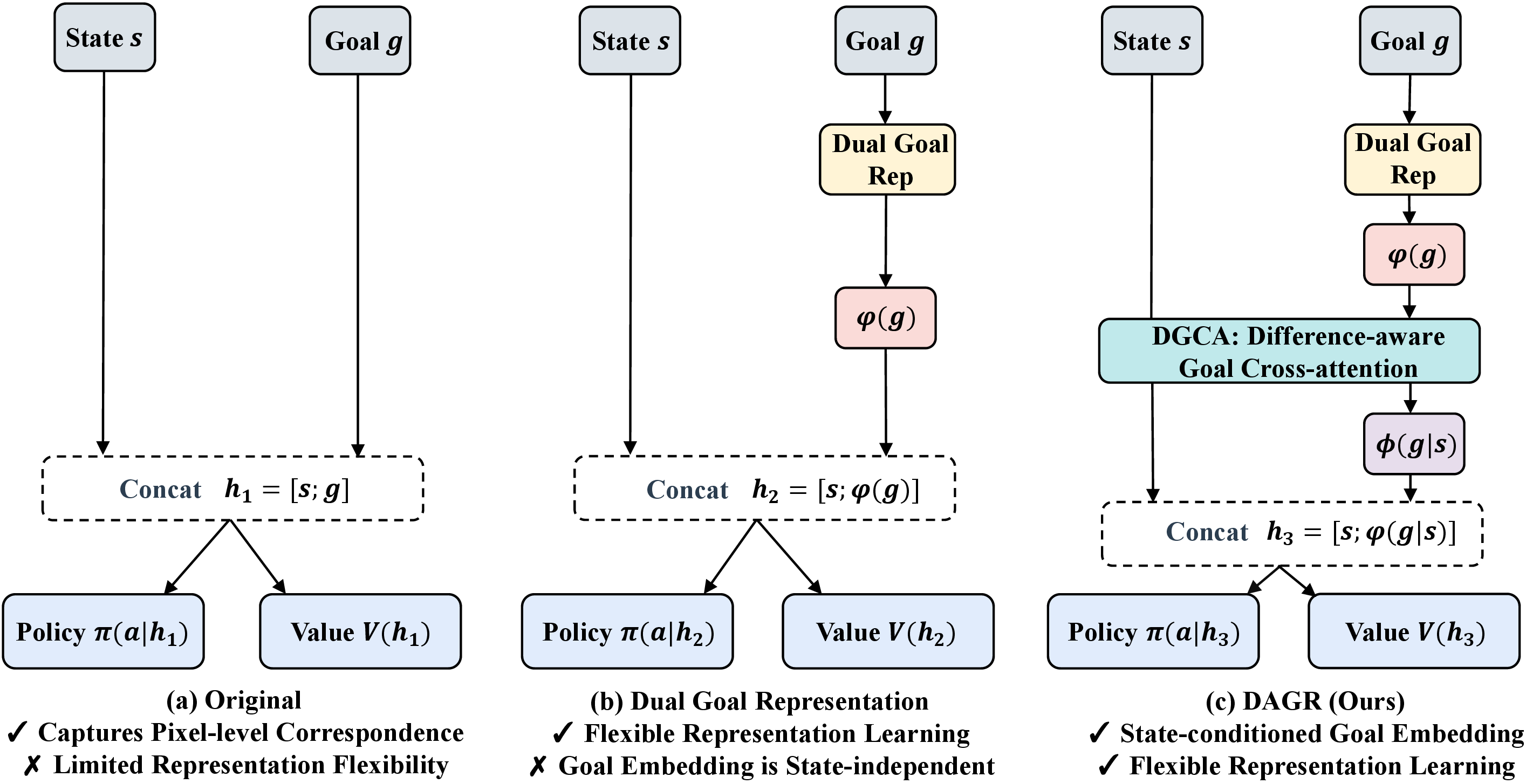
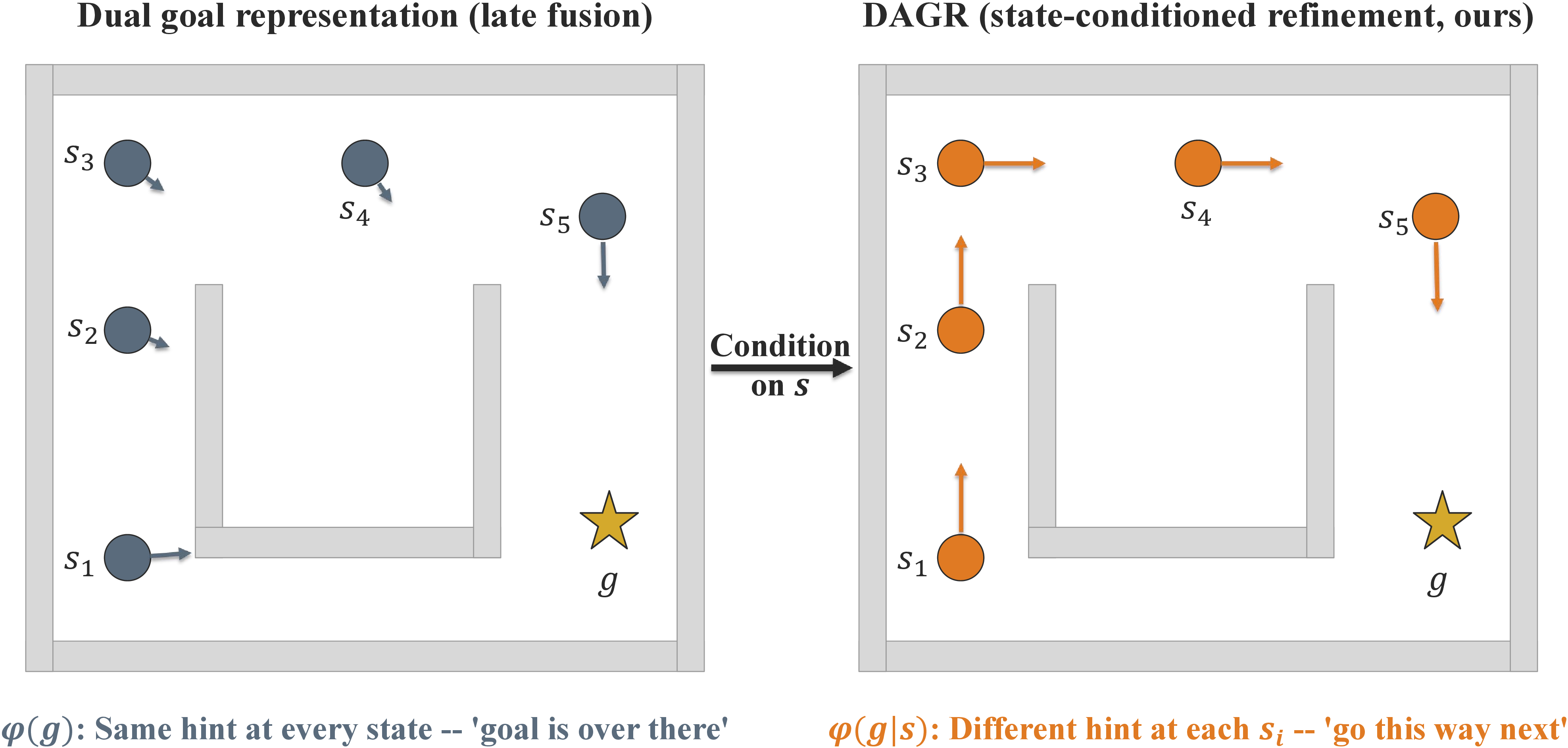
Figure 1: From a state-independent goal embedding to a state-conditioned one. The top panel contrasts the data flows of late fusion, Dual [21], and Dagr. The bottom panel shows the consequence in a shared maze with the same \(g\) and \(s_1, \ldots, s_5\). Under Dual, \(\phi(g)\) supplies the same hint at every \(s_i\). Under Dagr, the hint reflects the discrepancy between \(s_i\) and \(g\). Formally, Dagr defines the goal representation \(\varphi_{\mathrm{\mathrm{\small Dagr}{}}}^{\vee}(g \mid s)(s') = d^*(s', g) \cdot \Delta_{s, g}(s')\), where \(d^*(s', g)\) denotes the optimal temporal distance from \(s'\) to \(g\) and \(\Delta_{s, g} : \mathcal{S}\to[0, 1]\) weights the relevance of each \(s'\) to the current state-goal mismatch. This augments the Dual functional \(\varphi^{\vee}(g)(s') = d^*(s', g)\) with a state-dependent term, which is the property we call difference-aware. We approximate \(\Delta_{s, g}\) by the per-token discrepancy map of multi-scale Dgca in 4.2. What the figure isolates, and what our ablations confirm carries the gain, is the state-conditioning itself. The particular form of \(\Delta_{s, g}\) is a design choice on top of it..
We propose Dagr, a module that refines the static \(\phi(g)\) of any late-fusion encoder into a state-conditioned \(\phi(g \mid s)\) through cross-attention, as sketched in the top panel of 1. Refining a representation that already carries guarantees is delicate, so two choices keep it safe. The first is a multi-scale gated residual, initialized so that \(\phi(g \mid s)\) starts out equal to \(\phi(g)\). The downstream value and policy losses then shape a state-conditioned perturbation of the base, and they open the gate only where doing so pays. The second is an attention rule that adds a learnable non-negative bias, derived from a per-token state-goal difference map, to the usual similarity scores. 4 gives the architecture. It also shows that Dagr preserves the sufficiency and the noise invariance of any base representation (1 2), that the added approximation error stays under a gate-controlled bound (3), and that on discrepancy-structured tasks it admits a tighter sample-complexity upper bound than late fusion (3). We evaluate Dagr on OGBench [15], layered on Dual [21] with GCIVL [15] downstream. On state-based navigation it improves the success rate on every task but one, and the gains are largest on the mazes where Dual is weakest. On visual navigation it is the strongest of the six goal-representation baselines we compare against, so the directional signal survives the pixel encoder. The single exception is PointMaze, whose state is low-dimensional enough that the encoder barely compresses, and 3 predicts a null result exactly there. On manipulation and on the discrete puzzles the outcome is mixed. Dagr matches the base on some tasks and falls below it on others, and the tasks where it regresses are the ones that violate the structural condition of 3. Our ablations then ask which part of the module produces the gains that do appear, and the answer is not the part the method is named after. The gated residual carries the improvement, whereas removing the difference bias leaves navigation performance intact. We treat this as a finding rather than an inconvenience, and we state it in the main text.
Contributions. (i) We isolate the state-independence of the goal encoder as a design axis orthogonal to the choice of representation objective (2), and quantify its cost with an information bound and a Rademacher composition bound. (ii) We propose Dagr, a module that state-conditions any late-fusion goal encoder while provably retaining sufficiency, exogenous noise invariance, and a gate-controlled bound on the added value error. (iii) We state a structural condition on the task that predicts in advance where state-conditioning helps and where its optimum collapses back to the base, and both predictions hold on OGBench. (iv) We attribute the gain component by component, and report that the difference bias, which gives the module its name, contributes an inductive bias at initialization and little beyond it.
2 Related Work↩︎
Offline Goal-Conditioned RL. Offline GCRL trains goal-reaching policies from fixed datasets [11], [12]. Existing paradigms include behavioral cloning [9], [24], value-based estimation [15], [25], [26], hierarchical or subgoal-based planning [27]–[31], decision transformer [32], contrastive value learning [16], [17], [33], explicit subgoal planning [34], [35], dual optimization [36], [37], and generative trajectory modeling [38], [39]. OGBench [15] shows that no single method dominates across all task categories. Dagr is orthogonal to this axis, refining the goal representation consumed by any such downstream algorithm rather than proposing a new policy objective.
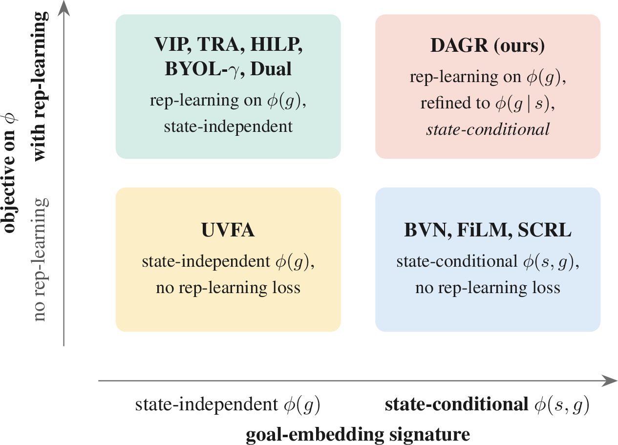
Figure 2: Two design axes for goal encoders in offline GCRL. Horizontal: whether \(\phi\) is state-conditional (\(\phi(s,g)\) or \(\phi(g\,|\,s)\)) or state-independent (\(\phi(g)\)). Vertical: whether \(\phi\) is trained with a representation-learning objective. Among these, Dagr is the only one that satisfies both. Quasimetric methods act on a third orthogonal axis (constraining the value-function class) and are omitted here..
Goal Representation Learning. Several families of objectives have been proposed for learning goal embeddings that generalize across unseen state-goal combinations [21], [40]. Metric-based methods align geometric and temporal distances (VIP [18], HILP [20], QRL [19] and its quasimetric extensions [41], [42]). Temporal-distance methods fit the embedding directly to a value or distance signal (TRA [43], Dual [21]). Information-theoretic methods compress the goal representation via a variational information bottleneck [22], [44], applied to GCRL by [23] and [27]. Self-predictive methods use bootstrapped temporal consistency in the form of BYOL-\(\gamma\) [45], building on the self-predictive representation framework of [46]. All such methods produce a state-independent \(\phi(g)\). Dagr is orthogonal and composable, as it operates on the output \(\phi(g)\) rather than on the objective that produces it.
Two axes prior work conflates. Goal representation learning shapes \(\phi\) through an auxiliary objective [18], [20], [21], [43], [45] but keeps it a function of \(g\) alone. A separate axis, often conflated with the first, asks whether \(\phi\) is state-conditional. UVFA [1] keeps \(\phi(g)\) state-independent, whereas BVN [47] uses \(\phi(s,g)\) and shows it to be strictly more expressive. FiLM [48] and SCRL [49] also condition on \(s\) but introduce no representation-learning objective. Dagr is closest in spirit to BVN on this axis but differs in three respects. First, it refines a representation-learned base \(\phi(g)\) rather than training \(\phi(s,g)\) monolithically. Second, it reduces to the base encoder at initialization through a gated residual that preserves sufficiency and noise invariance (1 2). Third, it biases attention with an explicit per-token difference map. A third orthogonal line constrains the value-function class to be quasimetric [19], [50]–[52], exploiting state-goal geometry on the value head rather than on \(\phi\). 2 summarizes these axes.
Cross-Attention in Computer Vision and RL. Cross-attention has become a standard mechanism for selective information flow across modalities in computer vision [53]–[55], with recent variants modifying the attention rule itself such as Gated Attention [56]. In RL, it underlies trajectory modeling [57], [58], in-context value inference [59], and an expanding body of work on vision-language-action models [60]–[67]. FiLM [48], [68] applies feature-wise modulation in goal-conditioned RL but is spatially uniform. To our knowledge, Dagr is the first to introduce a learnable difference bias into goal-conditioned cross-attention and to deploy it at multiple scales over a temporal-distance goal representation.
3 Preliminaries↩︎
3.1 Offline Goal-Conditioned RL↩︎
A goal-conditioned MDP (GCMDP) [69] is a tuple \(\mathcal{M}= (\mathcal{S}, \mathcal{A}, \mathcal{G}, p, r, \gamma)\) with goal space \(\mathcal{G}\subseteq \mathcal{S}\), sparse reward \(r(s, g) = \mathbb{1}[s = g]\), and discount \(\gamma \in (0, 1)\). A policy \(\pi : \mathcal{S}\times \mathcal{G}\to \Delta(\mathcal{A})\) induces value \(V^\pi(s, g) = \mathbb{E}_\pi[\sum_t \gamma^t r(s_t, g) \mid s_0 = s]\) with optimum \(V^*(s, g)\). We define the optimal temporal distance \(d^*(s, g) = \log_\gamma V^*(s, g)\), which equals the shortest-path length in deterministic environments. The offline dataset \(\mathcal{D}= \{(s_i, a_i, s'_i)\}_{i=1}^N\) is fixed.
3.2 Late Fusion and the State-Independence of \(\phi(g)\)↩︎
We focus on the late-fusion paradigm shared by current goal-representation methods (cf.1, left). A state encoder \(\psi : \mathcal{S}\to \mathbb{R}^{d_s}\) and a goal encoder \(\phi : \mathcal{G}\to \mathbb{R}^d\) are trained independently, and the policy is parameterized as \(\pi_\theta(a \mid \psi(s), \phi(g))\). The defining property of late fusion is that the goal encoder \(\phi\) takes no state input. For any fixed goal \(g\), the same vector \(\phi(g)\) is supplied to the policy and value heads regardless of the current state \(s\). The policy network must therefore infer at each step which components of \(\phi(g)\) are currently actionable. Dagr replaces \(\phi(g)\) by a state-conditioned \(\phi(g \mid s)\) that exposes this information explicitly at the representation level.2
Definition 1 (Sufficient Goal Representation [21]). A representation \(\phi : \mathcal{G}\to \mathbb{R}^d\) is sufficient for optimal control if there exists \(\pi^* : \mathcal{S}\times \mathbb{R}^d \to \Delta(\mathcal{A})\) such that \(V^{\pi^*(\cdot \mid s, \phi(g))}(s, g) = V^*(s, g)\) for all \((s, g) \in \mathcal{S}\times \mathcal{G}\).
3.3 Multi-Head Cross-Attention↩︎
Given \(Q \in \mathbb{R}^{n_q \times d}\), \(K \in \mathbb{R}^{n_k \times d}\), \(V \in \mathbb{R}^{n_k \times d_v}\), cross-attention is \(\mathrm{CrossAttn}(Q, K, V) = \mathrm{softmax}(QK^\top / \sqrt{d})\,V\) [70]. Multi-head attention computes \(H\) such operations in parallel with distinct projections \(W_h^Q, W_h^K, W_h^V\) and concatenates them through \(W^O\). The softmax weights measure similarity, so attention concentrates on tokens that resemble the query. For goal-conditioned control, the policy must act on the components in which state and goal disagree rather than on the components in which they agree. This mismatch between the inductive bias of standard cross-attention and the requirements of goal-conditioned control motivates the difference-bias term introduced in 4.
4 Difference-Aware Goal Representations↩︎
We begin with the core idea of Dagr, following the exposition pattern of the Dual representation [21]. Recall from 3 that the optimal temporal distance \(d^*(s, g) = \log_\gamma V^*(s, g)\) corresponds in deterministic environments to the shortest-path length from \(s\) to \(g\). The Dual representation characterizes a goal \(g\) by the set of optimal temporal distances \(d^*(\cdot, g)\) from all other states. In a discrete state space \(\mathcal{S}= \{s_1, \ldots, s_K\}\), this corresponds to the vector \[\varphi^{\vee}(g) \;=\; \big[d^*(s_1, g), \, d^*(s_2, g), \, \ldots, \, d^*(s_K, g)\big]^{\top}, \label{eq:dual95discrete}\tag{1}\] and in general to the functional \(\varphi^{\vee}(g)(s') = d^*(s', g)\), which depends on \(g\) alone. Dagr extends this construction with a state-dependent weighting: \[\varphi_{\mathrm{\mathrm{\small Dagr}{}}}^{\vee}(g \mid s) \;=\; \big[d^*(s_1, g)\cdot\Delta_{s, g}(s_1), \, \ldots, \, d^*(s_K, g)\cdot\Delta_{s, g}(s_K)\big]^{\top}, \label{eq:dagr95discrete}\tag{2}\] in the discrete case, and to the functional \(\varphi_{\mathrm{\mathrm{\small Dagr}{}}}^{\vee}(g \mid s)(s') = d^*(s', g) \cdot \Delta_{s, g}(s')\) in general. Here \(\Delta_{s, g} : \mathcal{S}\to [0, 1]\) is large when \(s'\) is informative about the difference between \(s\) and \(g\) and small when \(s'\) is irrelevant. We call \(\varphi_{\mathrm{\mathrm{\small Dagr}{}}}^{\vee}\) the difference-aware goal representation of the GCMDP \(\mathcal{M}\). In continuous environments we approximate \(\Delta_{s, g}\) by the per-token difference map of multi-scale Difference-aware Goal Cross-Attention in 4.2.
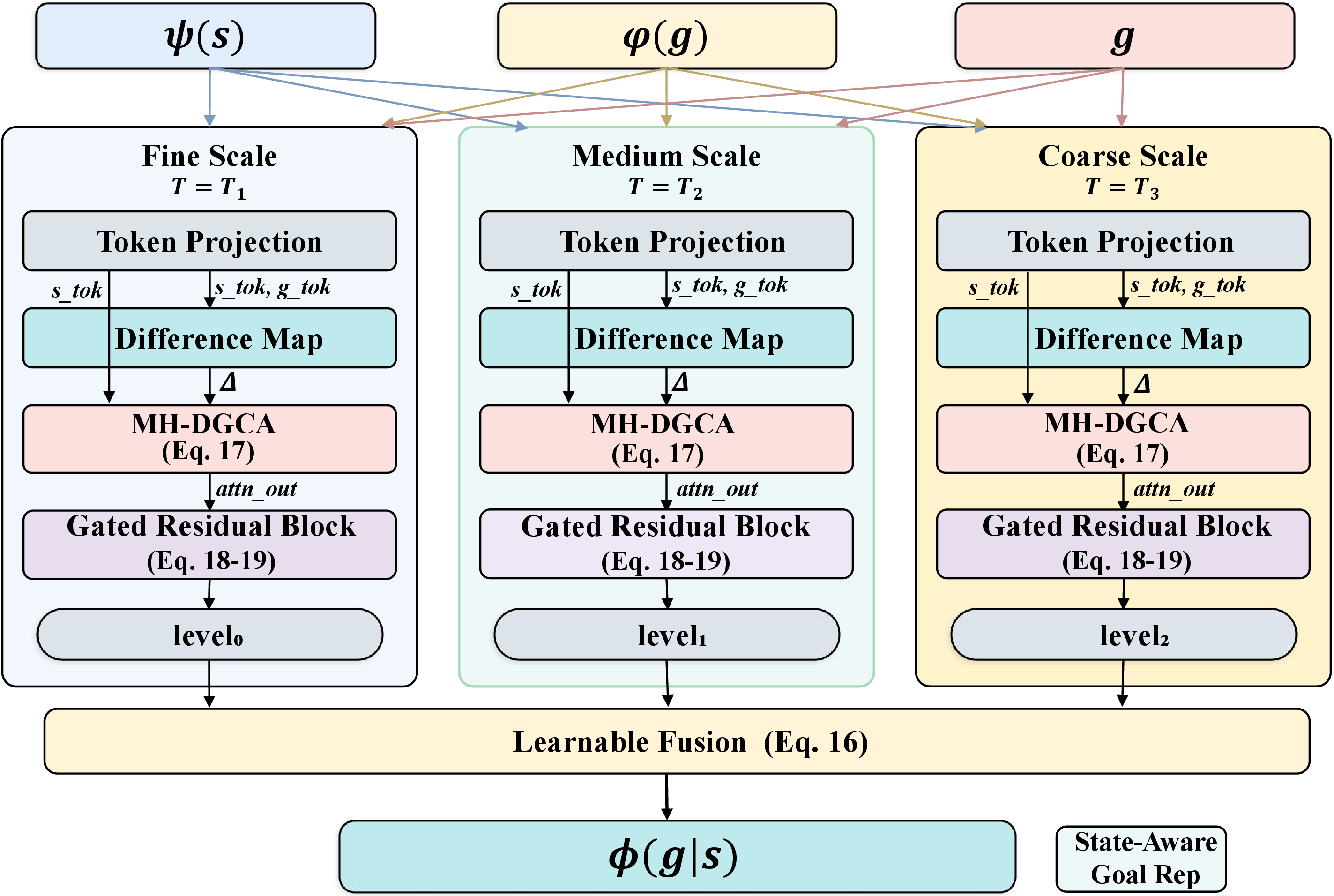
The rest of this section unpacks this construction. We first show what a state-independent goal representation cannot encode (4.1), then specify the single-scale (4.2) and multi-scale (4.3) DGCA blocks that realize \(\Delta_{s, g}\), and conclude with the theoretical properties of the resulting representation (4.4). The joint training procedure with the downstream offline GCRL algorithm is deferred to 7.
4.1 The Representation-Level Bottleneck of Late Fusion↩︎
To make precise what is missing in a state-independent \(\phi(g)\), let \(S\), \(G\), and \(A^*\) denote the random variables for state, goal, and optimal action. Under late fusion, conditioned on \(S = s\) the optimal action \(A^*\) is determined by \(\pi^*(\cdot \mid s, g)\), which depends on \(g\) only through \(\phi(g)\). This yields the Markov chain \(G \to \phi(G) \to A^*\) given \(S = s\), from which the data processing inequality yields the following bound.
Proposition 1 (Information Bottleneck of State-Independent Goal Representations). For any state-independent \(\phi\), \[I(A^* ; \phi(G) \mid S) \;\leq\; I(A^* ; G \mid S),\] with equality if and only if \(\phi(G)\) retains all goal information relevant to \(A^*\) given \(S\).
The equality condition fails precisely when the optimal action depends on a joint property of \((S, G)\) that \(\phi\) cannot resolve without access to \(S\). A canonical example is when \(\pi^*(a \mid s, g) = f(s - g)\), the relational case. Even when \(\phi\) is information-theoretically sufficient, the downstream policy still pays a sample-complexity price. Realizing \(\pi^*\) from inputs \((\psi(s), \phi(g))\) requires the network to implicitly invert both encoders before computing the difference. This composition is strictly harder than receiving \(s - g\) directly.
Proposition 2 (Late Fusion Admits a Looser Complexity Bound on Relational Tasks). Suppose \(\pi^*(a \mid s, g) = f(s - g)\). Then realizing \(\pi^*\) from the late-fusion inputs \((\psi(s), \phi(g))\) requires composing \(f\) with measurable inverse selections of \(\psi\) and of \(\phi\). The composition property of Rademacher complexity [71] then yields an upper bound on the policy class that exceeds the corresponding bound under direct access to \(s - g\) by a factor \(L_{\psi^{-1}} L_{\phi^{-1}} \geq 1\).
We are precise about what this does and does not say. It compares two upper bounds. It does not establish that the true Rademacher complexity of the realized function class is larger under late fusion. The proposition motivates the architecture. It does not prove that late fusion must be worse. Both observations point to the same fix: surface state-conditioned goal information at the representation level rather than asking the policy to recover it. This motivates the module we introduce next. Full proofs are in [app:proof_info_bottleneck] [app:proof_late_fusion_failure].
4.2 Single-Scale Difference-Aware Goal Cross-Attention (Dgca)↩︎
We aim to construct a transformation that takes the static \(\phi(g) \in \mathbb{R}^d\), the state encoding \(\psi(s) \in \mathbb{R}^{d_s}\), and a separate goal-image encoding \(\psi_g(g) \in \mathbb{R}^{d_s}\), and returns a state-conditioned representation \(\phi(g \mid s) \in \mathbb{R}^d\). The transformation should satisfy two properties. First, at initialization it should reduce to the identity map on \(\phi(g)\), so that training begins from the base representation. Second, it should be able to route information from state features that disagree with the goal into the refined representation. This routing is trainable end to end via the downstream policy and value losses.
The building block is a multi-head cross-attention in which the goal supplies the query and the state supplies the keys and values, with an additive bias derived from a per-token discrepancy map. 3 shows the architecture. Three ingredients realize it.
The first is a token decomposition. Let \(T\) denote the pseudo-token count, \(H\) the number of heads, \(d_k\) the per-head key dimension, and \(d_m := H d_k\). With separately learned projections \(W_s, W_g \in \mathbb{R}^{(T d_m) \times d_s}\), \[\mathbf{s}_\mathrm{tok} = \mathrm{Reshape}\big(W_s\, \psi(s)\big), \qquad \mathbf{g}_\mathrm{tok} = \mathrm{Reshape}\big(W_g\, \psi_g(g)\big) \;\in\; \mathbb{R}^{T \times d_m}. \label{eq:tokens}\tag{3}\] The two projections are untied, which aligns the token spaces position-wise and renders the per-token difference \(\mathbf{s}_\mathrm{tok}^{(t)} - \mathbf{g}_\mathrm{tok}^{(t)}\) meaningful.
The second ingredient is the difference map. A normalized \(\ell_2\) difference measures the mismatch at each token position, \[\Delta_t \;=\; \frac{\|\mathbf{s}_\mathrm{tok}^{(t)} - \mathbf{g}_\mathrm{tok}^{(t)}\|_2}{\max_{t'} \|\mathbf{s}_\mathrm{tok}^{(t')} - \mathbf{g}_\mathrm{tok}^{(t')}\|_2 + \varepsilon} \;\in\; [0, 1], \qquad \Delta = (\Delta_1, \ldots, \Delta_T), \label{eq:diff95map}\tag{4}\] with \(\varepsilon = 10^{-8}\) for numerical stability. The maximum is taken within the same \((s, g)\) pair, so \(\Delta\) ranks tokens by relative mismatch and is invariant to the absolute scale of state-goal differences. A value near one marks a position at which state and goal still differ, and a value near zero marks a position at which they agree.
The third ingredient is the attention rule that uses \(\Delta\) as an additive bias in logit space.
Definition 2 (Difference-Aware Goal Cross-Attention). Given a goal query \(Q \in \mathbb{R}^{1 \times d_k}\), state keys and values \(K, V \in \mathbb{R}^{T \times d_k}\), and a difference map \(\Delta \in [0, 1]^T\) as defined in 4 , \[\mathrm{DGCA}(Q, K, V, \Delta) \;=\; \mathrm{softmax}\left(\frac{Q K^\top}{\sqrt{d_k}} + \zeta(\lambda) \cdot \Delta\right) V \;\in\; \mathbb{R}^{1 \times d_k}, \label{eq:dgca}\tag{5}\] where \(\zeta : \mathbb{R}\to \mathbb{R}_{\geq 0}\) is defined by \(\zeta(x) := \mathrm{softplus}(x) = \log(1 + e^x)\), and \(\lambda \in \mathbb{R}\) is a learnable scalar parameter. We initialize \(\lambda_0 = -5\), which yields \(\zeta(\lambda_0) = \log(1 + e^{-5}) \approx 0.0067\).
The reparameterization through \(\zeta\) keeps the bias non-negative, so higher token-wise discrepancy only increases the corresponding attention logit. At initialization, \(\zeta(\lambda_0)\) is negligible and Dgca reduces to standard cross-attention. As \(\lambda\) grows during training, the bias additively boosts the logits of tokens with high \(\Delta_t\). A per-head \(\lambda_h\) lets different heads specialize at different bias intensities.
The multi-head version applies \(H\) parallel heads with projections \(W_h^Q \in \mathbb{R}^{d \times d_k}\) for the goal query and \(W_h^K, W_h^V \in \mathbb{R}^{d_m \times d_k}\) for the state tokens, \[\mathrm{head}_h = \mathrm{softmax}\left(\tfrac{\phi(g)W_h^Q (\mathbf{s}_\mathrm{tok}W_h^K)^\top}{\sqrt{d_k}} + \zeta(\lambda_h)\Delta\right)\mathbf{s}_\mathrm{tok}W_h^V, \quad \mathrm{attn\_out} = \mathrm{Concat}_h(\mathrm{head}_h)\, W^O, \label{eq:mhdgca}\tag{6}\] with \(W^O \in \mathbb{R}^{(H d_k) \times d}\) and a per-head \(\lambda_h\) that permits different heads to adopt different bias intensities. The attention output is integrated into the goal representation through a gated residual block, followed by layer normalization and a feed-forward network with its own gated residual, \[\begin{align} \mathbf{x} &= \phi(g) + \sigma(\alpha_\mathrm{attn}) \odot \mathrm{attn\_out}, & \mathbf{x} &\leftarrow \mathrm{LayerNorm}(\mathbf{x}), \tag{7} \\ \mathrm{out} &= \mathbf{x} + \sigma(\alpha_\mathrm{ffn}) \odot \mathrm{FFN}(\mathbf{x}), & \mathrm{out} &\leftarrow \mathrm{LayerNorm}(\mathrm{out}), \tag{8} \end{align}\] Here \(\sigma\) is the elementwise sigmoid, \(\odot\) the Hadamard product, and \(\mathrm{FFN}\) a two-layer network with GELU activation. The gate vectors \(\alpha_\mathrm{attn}, \alpha_\mathrm{ffn} \in \mathbb{R}^d\) are initialized componentwise to \(-5\), which yields \(\sigma(\alpha) \approx 0.0067\). Vector-valued gates permit each coordinate of the goal representation to be modulated independently. We write \(\mathrm{DGCA\text{-}Block}_T(\phi(g), \psi(s), \psi_g(g))\) for the output of 8 .
The gates start nearly closed, so \(\phi(g \mid s) \approx \phi(g)\) and the temporal-distance structure of the base survives. They open during training only where doing so reduces the downstream losses, which yields an automatic curriculum from late fusion to state-conditioned refinement.
4.3 Multi-Scale Extension↩︎
A single token count \(T\) commits the module to one analysis granularity. In practice, the spatial scale at which state-goal discrepancies are informative varies across tasks. Navigation often hinges on coarse global offsets, while manipulation may depend on a small object-level mismatch. We therefore apply \(L\) independent Dgca blocks at decreasing token counts \(T_1 > T_2 > \cdots > T_L\), each with its own token projections and attention parameters, and combine them through learnable fusion weights, \[\mathrm{level}_\ell \;=\; \mathrm{DGCA}\text{-}\mathrm{Block}_{T_\ell}\big(\phi(g),\, \psi(s),\, \psi_g(g)\big), \qquad \phi_{\mathrm{\mathrm{\small Dagr}{}}}(g \mid s) \;=\; \sum_{\ell=1}^{L} \mathrm{softmax}(w)_\ell \cdot \mathrm{level}_\ell. \label{eq:ms95fusion}\tag{9}\] The fusion logits \(w \in \mathbb{R}^L\) are initialized to zero so that all scales contribute equally at the start. We use \(L = 3\) with \((T_1, T_2, T_3) = (16, 8, 4)\) throughout the paper. Fine scales (large \(T\)) carry local information, coarse scales (small \(T\)) aggregate global structure, and the data-driven \(w\) trades off between them based on the downstream loss. Dagr is trained jointly with the downstream offline GCRL algorithm through standard value and policy losses propagated through multi-scale Dgca (MS-Dgca), with the full procedure (4) given in 7.
4.4 Theoretical Properties↩︎
We state five properties. Three are safety guarantees that hold on any task. Two tie the value of refinement to the following structural condition.
Definition 3 (Discrepancy Structure). A goal-conditioned task with optimal policy \(\pi^*\) has discrepancy structure if there exists a measurable function \(h : \mathcal{S}\times \mathcal{S}\to \mathcal{Z}\) and a measurable function \(\rho : \mathcal{Z}\to \Delta(\mathcal{A})\) such that \[\pi^*(a \mid s, g) = \rho\big(h(s, g)\big) \quad \text{for all } (s, g) \in \mathcal{S}\times \mathcal{G}, \label{eq:discrepancy}\tag{10}\] and such that \(h\) is not a function of \(g\) alone. We call \(h\) the discrepancy map. A task admitting 10 with \(h\) a function of \(g\) alone is called goal-only.
Throughout, we treat \(\phi\), \(\psi\), and \(\psi_g\) as fixed and consider the map \(\phi(g) \mapsto \phi_{\mathrm{\mathrm{\small Dagr}{}}}(g \mid s)\) for any fixed \(s \in \mathcal{S}\). Full statements and proofs are deferred to 10.
A base representation that is already sufficient stays sufficient after refinement, because each scale block is an injective perturbation of the identity.
Theorem 1 (Sufficiency Preservation). Assume \(\phi\) is sufficient (1), that the residual perturbation \(\delta_\ell\) of each scale is \(L_\ell\)-Lipschitz in \(\phi(g)\) with \(\|\sigma(\alpha)\|_\infty L_\ell < 1\), and that the in-block normalization is injective on the range of \(\phi\). Then \(\phi_{\mathrm{\mathrm{\small Dagr}{}}}(\cdot \mid s)\) is sufficient.
The contraction condition holds on every run we instrument (6). The injectivity condition does not. 7 8 normalize the output of each sub-block, and LayerNorm discards the mean and the scale of its input. 1 therefore certifies the gate and the attention but not the normalization we place after them. We flag the gap here and return to it in 6, where the same architectural detail turns out to be our leading explanation for the manipulation regression.
Noise invariance carries over more cleanly. Every node of the MS-Dgca graph touches the goal observation only through \(\phi\) and \(\psi_g\), so their invariance propagates.
Theorem 2 (Noise Invariance Preservation). Suppose goal observations decompose as \(o_g = (x_g, \epsilon_g)\) with \(\epsilon_g\) task-irrelevant, and suppose the base encoders satisfy \(\phi(o_g) = \phi(x_g)\) and \(\psi_g(o_g) = \psi_g(x_g)\) for all \((x_g, \epsilon_g)\). Then \(\phi_{\mathrm{\mathrm{\small Dagr}{}}}(o_g \mid s) = \phi_{\mathrm{\mathrm{\small Dagr}{}}}(x_g \mid s)\) for every \(\epsilon_g\) and every \(s \in \mathcal{S}\).
The third property bounds the worst-case cost of the added expressiveness.
Theorem 3 (Approximation Error Bound). Let \(f : \mathbb{R}^{d_s} \times \mathbb{R}^d \to \mathbb{R}\) be \(L_V\)-Lipschitz in its second argument, and suppose \(\|\phi_{\mathrm{\mathrm{\small Dagr}{}}}(g \mid s) - \phi(g)\|_2 \leq B\) holds uniformly over \((s, g) \in \mathcal{S}\times \mathcal{G}\). Define \(\varepsilon_\mathrm{base} := \sup_{(s, g) \in \mathcal{S}\times \mathcal{G}} |V^*(s, g) - f(\psi(s), \phi(g))|\) and \(\hat{V}(s, g) := f(\psi(s), \phi_{\mathrm{\mathrm{\small Dagr}{}}}(g \mid s))\). Then \[\sup_{(s, g) \in \mathcal{S}\times \mathcal{G}} |V^*(s, g) - \hat{V}(s, g)| \;\leq\; \varepsilon_\mathrm{base} + L_V \cdot B. \label{eq:approx95bound}\tag{11}\]
At initialization the gates are near zero, so \(B \approx 0\) and the bound reduces to that of the base. It grows only as the optimizer opens the gates. We claim no more than that the upper bound is gate-controlled, and 1 shows why that is less than it sounds.
The remaining two properties tie the value of refinement to 3.
Proposition 3 (Tighter Sample-Complexity Bound on Discrepancy-Structured Tasks). Suppose the task has discrepancy structure 10 with discrepancy map \(h\), and suppose that the pair \((\psi, \phi_{\mathrm{\mathrm{\small Dagr}{}}})\) realizes \(h\) in the sense that there exists an \(L_h\)-Lipschitz \(\tilde{h} : \mathbb{R}^{d_s} \times \mathbb{R}^d \to \mathcal{Z}\) with \(\tilde{h}(\psi(s), \phi_{\mathrm{\mathrm{\small Dagr}{}}}(g \mid s)) = h(s, g)\), while no \(L_h\)-Lipschitz function on \((\psi(s), \phi(g))\) realizes \(h\). Let \(\pi^* = \rho \circ h\) with \(\rho\) Lipschitz. The standard Rademacher composition bound [71] then yields data-dependent upper bounds \(U_n^{\mathrm{late}}\) and \(U_n^{\mathrm{\small Dagr}{}}\) on \(\mathfrak{R}_n\) of the policy class that satisfy \[U_n^{\mathrm{\small Dagr}{}} \;\leq\; L_h \cdot L_\rho \cdot \mathfrak{R}_n(\mathcal{H}_\rho), \qquad U_n^{\mathrm{late}} \;\leq\; L_{\psi^{-1}} \cdot L_{\phi^{-1}} \cdot L_h \cdot L_\rho \cdot \mathfrak{R}_n(\mathcal{H}_\rho), \label{eq:rad95gap}\qquad{(1)}\] where \(L_{\psi^{-1}}, L_{\phi^{-1}} \geq 1\) are the Lipschitz constants of any measurable selections inverting \(\psi\) and \(\phi\), and \(\mathcal{H}_\rho\) denotes the policy class realizing \(\rho\). The DAGR bound is therefore tighter by a multiplicative factor \(L_{\psi^{-1}} L_{\phi^{-1}}\).
The proof extends 2 from \(h(s, g) = s - g\) to arbitrary discrepancy maps, and the intuition is unchanged. Dagr exposes \(h\) at the representation level, while late fusion must recover it by inverting both encoders. The bound rests on a realizability assumption that we do not verify directly, and our gains are consistent with it but do not establish it. 9 states the assumption precisely and names the probe experiment that would settle it.
Proposition 4 (Reduction to Base on Goal-Only Tasks). If the task is goal-only in the sense of 3, that is, \(\pi^*(a \mid s, g) = \rho(\bar h(g))\) for some \(\bar h\) depending only on \(g\), and if the base representation \(\phi\) is sufficient (1) for \(\pi^*\) with \(\rho \circ \bar h \in \mathcal{F}_{\mathrm{late}}\), then the global minimum of any value or policy loss in \(\mathcal{F}_{\mathrm{\mathrm{\small Dagr}{}}}\) that achieves the base error \(\varepsilon_{\mathrm{base}}\) is attained at gate parameters \(\alpha, \lambda_h \to -\infty\), equivalently at \(B = 0\) in 3 and at \(\phi_{\mathrm{\mathrm{\small Dagr}{}}}(g \mid s) \equiv \phi(g)\).
The two propositions together mark the regime where Dagr formally helps and the regime where its best behavior is to reduce to the base. The next remark asks whether it does.
Remark 1 (What the Bound Does and Does Not Explain). Read together, 4 3 predict that a goal-only task pays a penalty proportional to its converged gate. That prediction fails on our data, and we report the failure rather than force the fit. On Cube-Double the gates stay below \(0.01\) (7), so \(B\) and the certified surcharge \(L_V \cdot B\) are both small, yet the success rate falls by \(25\) points. [tbl:tab:sensitivities] shows the mismatch from the other side. Opening the gates at initialization raises \(B\) by two orders of magnitude and costs only \(8\) points. A large \(B\) therefore hurts less than a small one, which no monotone reading of 3 allows. The bound still does its job, since it certifies that the refinement cannot blow up at any gate value we observe. It is simply not the mechanism behind the regression, and we do not present it as one. 6 names the mechanism.
5 Experiments↩︎
We evaluate Dagr on OGBench [15] along three axes. First, whether state-conditioned refinement improves goal reaching across diverse tasks. Second, whether the difference bias contributes beyond standard cross-attention. Third, on which tasks it does not help, and why.
Setup. We evaluate on 13 state-based tasks and 7 visual variants. The state-based tasks comprise navigation tasks (PointMaze, AntMaze, HumanoidMaze, and AntSoccer), manipulation tasks (Cube-Single, Cube-Double, and Scene), and discrete-reasoning tasks (Puzzle-3x3 and Puzzle-4x4). The base goal representation is Dual [21] with bilinear (inner-product) parameterization, and the downstream offline GCRL algorithm is GCIVL [15]. Dagr uses \(H = 4\) heads with \(d_k = 64\), scales \((T_1, T_2, T_3) = (16, 8, 4)\), FFN hidden dimension \(256\), and one Dgca block per scale. All gate parameters and difference scalings are initialized to \(\alpha_0 = \lambda_0 = -5\), and fusion logits to zero. We use eight seeds for state-based tasks and four seeds for visual tasks. Full hyperparameters are in 5 of 11. The Orig, VIB, VIP, TRA, BYOL-\(\gamma\), and Dual numbers are reproduced from [21] under their own tuned settings. Dagr uses a single fixed configuration across all tasks rather than per-task tuning. The reported gains are therefore not attributable to task-specific hyperparameter search.
5.1 Main Results: State-Based Tasks↩︎
| Environment | Orig | VIB | VIP | TRA | BYOL-\(\gamma\) | Dual | |
|---|---|---|---|---|---|---|---|
| Navigation | |||||||
| pointmaze-medium-navigate | 78\(\pm\)8 | 69\(\pm\)13 | 0\(\pm\)1 | 3\(\pm\)6 | 37\(\pm\)7 | 76\(\pm\)7 | 87\(\pm\)8 |
| pointmaze-large-navigate | 52\(\pm\)6 | 50\(\pm\)7 | 0\(\pm\)0 | 1\(\pm\)2 | 22\(\pm\)12 | 46\(\pm\)6 | 41\(\pm\)7 |
| antmaze-medium-navigate | 71\(\pm\)4 | 68\(\pm\)4 | 31\(\pm\)5 | 22\(\pm\)15 | 39\(\pm\)5 | 75\(\pm\)4 | 95\(\pm\)1 |
| antmaze-large-navigate | 16\(\pm\)3 | 9\(\pm\)3 | 9\(\pm\)2 | 22\(\pm\)12 | 11\(\pm\)5 | 28\(\pm\)11 | 82\(\pm\)3 |
| antmaze-giant-navigate | 0\(\pm\)0 | 0\(\pm\)0 | 0\(\pm\)0 | 0\(\pm\)0 | 0\(\pm\)0 | 0\(\pm\)0 | 4\(\pm\)2 |
| humanoidmaze-medium-navigate | 27\(\pm\)3 | 24\(\pm\)2 | 7\(\pm\)3 | 21\(\pm\)3 | 18\(\pm\)5 | 29\(\pm\)3 | 83\(\pm\)3 |
| humanoidmaze-large-navigate | 3\(\pm\)0 | 3\(\pm\)1 | 1\(\pm\)0 | 2\(\pm\)1 | 2\(\pm\)1 | 3\(\pm\)2 | 62\(\pm\)4 |
| antsoccer-arena-navigate | 47\(\pm\)4 | 34\(\pm\)4 | 2\(\pm\)1 | 8\(\pm\)2 | 11\(\pm\)4 | 31\(\pm\)3 | 58\(\pm\)4 |
| Manipulation | |||||||
| cube-single-play | 52\(\pm\)3 | 90\(\pm\)3 | 40\(\pm\)7 | 40\(\pm\)5 | 51\(\pm\)11 | 89\(\pm\)3 | 87\(\pm\)2 |
| cube-double-play | 35\(\pm\)5 | 33\(\pm\)3 | 3\(\pm\)2 | 7\(\pm\)2 | 6\(\pm\)4 | 60\(\pm\)4 | 35\(\pm\)2 |
| scene-play | 46\(\pm\)3 | 58\(\pm\)1 | 23\(\pm\)6 | 46\(\pm\)6 | 44\(\pm\)9 | 72\(\pm\)6 | 59\(\pm\)2 |
| Discrete Reasoning | |||||||
| puzzle-3x3-play | 5\(\pm\)1 | 14\(\pm\)3 | 3\(\pm\)1 | 5\(\pm\)1 | 0\(\pm\)0 | 5\(\pm\)1 | 5\(\pm\)1 |
| puzzle-4x4-play | 14\(\pm\)1 | 6\(\pm\)3 | 1\(\pm\)1 | 10\(\pm\)3 | 1\(\pm\)2 | 23\(\pm\)3 | 14\(\pm\)3 |
| Average | 34\(\pm\)1 | 35\(\pm\)2 | 9\(\pm\)1 | 15\(\pm\)2 | 19\(\pm\)2 | 41\(\pm\)2 | 55 |
1 reports the state-based results. The pattern is highly structured. On every navigation task except pointmaze-large, Dagr attains the best or tied-best score, with the largest absolute gains where Dual is weakest. These tasks fit 3 with \(h(s, g) = \pi_{xy}(s) - \pi_{xy}(g)\), the position offset. 3 therefore gives a tighter sample-complexity upper bound on these tasks, consistent with the early-training separation we observe in 9.
On manipulation the picture is mixed. Cube-Single matches Dual. Cube-Double and Scene fall below it. Neither of the latter two fits 3. On Cube-Double the optimal action turns on a binary choice of which cube to move first. On Scene it turns on a multi-step ordering decision. Neither factors through a discrepancy map \(h(s, g)\), so 4 applies, and it predicts that the best Dagr can do on these tasks is to match Dual by closing its gates.
The gates do stay nearly closed. 7 shows \(\sigma(\alpha)\) below \(0.01\) throughout. What 4 does not predict, and what we observe, is a \(25\)-point drop. 1 works through why the gate-controlled bound of 3 cannot supply the missing \(25\) points. We therefore report the regression as an open failure of our account rather than as a confirmation of it. 6 gives our leading hypothesis. On puzzle the gap to Dual is essentially zero, because no late-fusion representation method we evaluate reaches a non-trivial success rate at all (12.4). Full training curves are in 9.
5.2 Main Results: Visual Tasks↩︎
| Environment | Orig | VIB | VIP | TRA | BYOL-\(\gamma\) | Dual | (Ours) |
|---|---|---|---|---|---|---|---|
| Navigation | |||||||
| visual-antmaze-medium-navigate | 66\(\pm\)4 | 18\(\pm\)9 | 30\(\pm\)7 | 48\(\pm\)4 | 32\(\pm\)5 | 78\(\pm\)4 | 90\(\pm\)2 |
| visual-antmaze-large-navigate | 26\(\pm\)5 | 5\(\pm\)2 | 9\(\pm\)1 | 13\(\pm\)3 | 9\(\pm\)4 | 40\(\pm\)4 | 52\(\pm\)2 |
| Manipulation | |||||||
| visual-cube-single-play | 53\(\pm\)4 | 18\(\pm\)19 | 39\(\pm\)6 | 31\(\pm\)24 | 35\(\pm\)8 | 58\(\pm\)5 | 44\(\pm\)2 |
| visual-cube-double-play | 9\(\pm\)2 | 0\(\pm\)0 | 0\(\pm\)0 | 3\(\pm\)2 | 2\(\pm\)1 | 9\(\pm\)2 | 11\(\pm\)4 |
| visual-scene-play | 25\(\pm\)2 | 6\(\pm\)3 | 4\(\pm\)1 | 15\(\pm\)6 | 10\(\pm\)8 | 26\(\pm\)5 | 27\(\pm\)3 |
| Discrete Reasoning | |||||||
| visual-puzzle-3x3-play | 22\(\pm\)2 | 0\(\pm\)0 | 0\(\pm\)0 | 0\(\pm\)0 | 0\(\pm\)0 | 0\(\pm\)0 | 0\(\pm\)0 |
| visual-puzzle-4x4-play | 65\(\pm\)4 | 0\(\pm\)0 | 0\(\pm\)0 | 0\(\pm\)0 | 0\(\pm\)0 | 0\(\pm\)0 | 0\(\pm\)0 |
| Avg.(all 7 tasks) | 38 | 7 | 12 | 16 | 13 | 30 | 32 |
| Avg.(excl.puzzle) | 36 | 9 | 16 | 22 | 18 | 42 | 45 |
2 reproduces the state-based pattern on navigation. Dagr is highest on both Visual-AntMaze variants, so the directional signal survives the pixel encoder. Visual manipulation splits. Cube-Double and Scene match Dual, whereas Cube-Single falls below it, and 5.3 identifies this as the one task on which state-conditioning helps but our attention rule does not. Visual-Puzzle remains at zero for every late-fusion method, an encoder-level bottleneck we examine in 12.4. Curves are in 10.
5.3 Ablation: Standard Cross-Attention vs.Dgca↩︎
| Environment | Dual | +CA | + |
|---|---|---|---|
| State-Based | |||
| antmaze-medium | 75\(\pm\)4 | 84\(\pm\)6 | 95\(\pm\)1 |
| antmaze-large | 28\(\pm\)11 | 33\(\pm\)4 | 82\(\pm\)3 |
| humanoidmaze-medium | 29\(\pm\)3 | 41\(\pm\)7 | 83\(\pm\)3 |
| humanoidmaze-large | 3\(\pm\)2 | 8\(\pm\)2 | 62\(\pm\)4 |
| antsoccer-arena | 31\(\pm\)3 | 44\(\pm\)2 | 58\(\pm\)4 |
| cube-double | 60\(\pm\)4 | 26\(\pm\)5 | 35\(\pm\)2 |
| scene | 72\(\pm\)6 | 57\(\pm\)1 | 59\(\pm\)2 |
| Visual | |||
| visual-antmaze-medium | 78\(\pm\)4 | 80\(\pm\)14 | 90\(\pm\)2 |
| visual-antmaze-large | 40\(\pm\)4 | 41\(\pm\)9 | 52\(\pm\)2 |
| visual-cube-single | 58\(\pm\)5 | 80\(\pm\)3 | 44\(\pm\)2 |
| visual-cube-double | 9\(\pm\)2 | 10\(\pm\)2 | 11\(\pm\)4 |
| visual-scene | 26\(\pm\)5 | 13\(\pm\)2 | 27\(\pm\)3 |
| visual-puzzle-3x3 | 0\(\pm\)0 | 0\(\pm\)0 | 0\(\pm\)0 |
3 compares Dual, Dual with a standard cross-attention module (+CA, single-scale, gate at \(\sigma(0) = 0.5\), no difference bias), and Dual with the full Dgca. On navigation, Dgca clearly beats +CA, and the gap is widest where Dual is weakest. The two differ in two ways at once, since Dgca adds the difference bias and it closes the gate at initialization. ¿tbl:tab:ablation95components? separates them. Removing the difference bias from Dgca leaves AntMaze-Large at \(84.4\), which is not below the full model at \(82.5\). Removing the gated residual drops it to \(59.3\). The gate, not the bias, is what +CA is missing. We state this plainly. The mechanism that names our method is not the mechanism that produces our navigation gains.
Visual-Cube-Single is the sharpest counterexample in the paper, and we treat it as one. +CA reaches \(80\) there against \(58\) for Dual and \(44\) for Dgca. Two readings follow, and they point in opposite directions. State-conditioning helps a great deal on this task, and the \(+22\) points +CA gains over Dual is the largest single-task gain any module produces anywhere in this paper, so the failure is not on the state-conditional axis. Yet the two ingredients that separate Dgca from +CA are jointly harmful here, and together they cost \(36\) points. We cannot separate their contributions with the ablations we have. One untested account is that single-object visual goal reaching is a template-matching problem, for which similarity-maximizing attention is the correct bias and a discrepancy-maximizing one is not. On Cube-Double and Scene both variants fall below Dual, consistent with 5.1.
5.4 Component Attribution and Scope↩︎
¿tbl:tab:ablation95components? of 12 isolates each component of MS-Dgca. Three results matter here. Removing the gated residual drops AntMaze-Large from \(82.5\) to \(59.3\), which confirms that the near-identity initialization protects the base temporal-distance structure. Removing the difference bias leaves it at \(84.4\), within one standard deviation of the full model. Removing the FFN drops it to \(57.7\). The gate and the per-token projection therefore carry the navigation gain, and the difference bias does not.
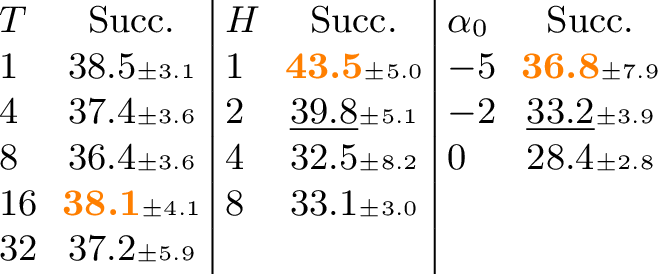
7 of 12 explains why. The learned \(\zeta(\lambda)\) remains at its initialization value on five of six tasks, so the bias never activates at convergence. 6 shows the same for the gates, which stay below \(0.01\) throughout. Dagr therefore operates as a small, gated perturbation of \(\phi(g)\), and the difference bias supplies an inductive prior at initialization rather than a converged contribution. [tbl:tab:sensitivities] confirms the protective reading of the gate. Initializing \(\alpha_0 = 0\) rather than \(-5\) opens the gates from the first gradient step and costs \(8\) points on Cube-Double.
6 of 12 delimits the scope. Every late-fusion representation method, ours included, scores zero on Visual-Puzzle, whereas vanilla GCIVL under early fusion does not. The bottleneck lies in the encoder rather than in \(\phi\), since the IMPALA CNN pools away the pixel-level correspondence between the state and goal images before \(\phi(g)\) is computed. A post-encoder module can only reweight what the encoder preserves.
6 Conclusion and Discussion↩︎
Dagr refines a static goal embedding into a gated, multi-scale, state-conditioned one. It preserves sufficiency and noise invariance, tightens the sample-complexity bound on discrepancy-structured tasks, and improves goal reaching on every navigation task that 3 covers. The ablations attribute that improvement to the gated residual rather than to the difference bias the method is named for.
The regression on Cube-Double and Scene is architectural. 7 8 normalize each sub-block output, so a closed gate discards the norm of the base embedding, on which the bilinear temporal distance of Dual depends. Navigation reads direction alone and is unaffected, whereas manipulation is not. ¿tbl:tab:ablation95components? supports this, since removing the normalization recovers Cube-Double while leaving AntMaze-Large within noise. Pre-normalizing each sub-block would restore exact identity and close the injectivity gap in 1. Two limitations remain. The token decomposition is not object-aware, which plausibly compounds the manipulation deficit, and the Visual-Puzzle failure lies in the encoder rather than the goal representation, where hierarchical planning [27] is complementary.
1.5
7 Training Procedure↩︎
Dagr is trained jointly with the downstream offline GCRL algorithm. The base representation loss \(\mathcal{L}_{\mathrm{rep}}\) produces \(\phi(g)\) without cross-attention, exactly as in the underlying Dual method, so the temporal-distance structure of \(\phi\) relied on by 1 2 is not perturbed. Only the value, Q, and policy losses propagate gradients through MS-Dgca. Its parameters comprise the per-scale token projections \(\{W_s^{(\ell)}, W_g^{(\ell)}\}\) (3 ), attention matrices \(\{W_h^{Q,(\ell)}, W_h^{K,(\ell)}, W_h^{V,(\ell)}, W^{O,(\ell)}\}\) (6 ), gate vectors \(\{\alpha_{\mathrm{attn}}^{(\ell)}, \alpha_{\mathrm{ffn}}^{(\ell)}\}\) and per-head difference scalars \(\{\lambda_h^{(\ell)}\}\) (7 8 5 ), per-scale FFN parameters, and fusion logits \(w \in \mathbb{R}^L\) (9 ). Each call \(\mathrm{MS\text{-}\mathrm{\small Dgca}{}}(\phi(g), \psi(s), \psi_g(g))\) proceeds in four steps. Step (i) projects \(\psi(s), \psi_g(g)\) into pseudo-tokens via 3 . Step (ii) computes the difference map via 4 . Step (iii) runs multi-head Dgca and the gated residual block via 6 7 8 at each of \(L\) scales. Step (iv) fuses the scale outputs via 9 . The near-zero gate initialization ensures \(\tilde{\phi} \approx \phi(g)\) at step zero. Gates open only when doing so reduces the downstream losses, which realizes the late-fusion-to-refinement curriculum discussed in 4.2 and bounded by 3.
![Figure 4: Dagr layered on top of the Dual goal representation [21] with GCIVL [15], [26] as the downstream offline GCRL algorithm. Lines highlighted in orange mark the differences from a plain Dual + GCIVL baseline.](/article/2607.13731/_pdflatex/vdbwfznk.png "fig:")
8 Notation↩︎
| Symbol | Description |
|---|---|
| General notation | |
| \(\phi(g\mid s)\) | Deterministic state-parameterized goal encoding; the bar denotes parameter dependence, not a conditional distribution. Equivalently \(\phi(g;s)\) or \(\phi_s(g)\). |
| \(\varphi^\vee(g),\;\varphi_{\textup{\DAGR{}}}^\vee(g\mid s)\) | Dual and goal functionals from \(\cS\) to \(\RR\) ([eq:dual95discrete] [eq:dagr95discrete]); the latter is \(\Delta_{s,g}\)-weighted version of the former. |
| \(d^*(s,g)\) | Optimal temporal distance \(\log_\gamma V^*(s,g)\) ([sec:sec:prelim]); equals shortest-path length in deterministic environments. |
| \(\Delta_{s,g}(\cdot)\) | State-dependent weighting \(\cS\to[0,1]\) in the functional ([eq:dagr95discrete]); approximated by the per-token discrepancy map \(\Delta_t\) of [eq:diff95map]. |
| \(h(s,g),\;\rho\) | Discrepancy map \(\cS\times\cS\to\cZ\) and corresponding policy factor \(\cZ\to\Delta(\cA)\) such that \(\pi^*(a\mid s,g)=\rho(h(s,g))\). |
| \(\cZ\) | Latent discrepancy space; concrete instances include \(\RR^k\) (e.g., \(h(s,g)=\pi_{xy}(s)-\pi_{xy}(g)\) for maze navigation). |
| “goal-only” | Task satisfying [eq:discrepancy] with \(h\) a function of \(g\) alone, that is, \(\pi^*(a\mid s,g)=\rho(\bar h(g))\) for some \(\bar h\). |
| \(S, G, A^*\) | Random variables for state, goal, and optimal action. |
| \(I(X;Y\mid Z)\) | Conditional mutual information between \(X\) and \(Y\) given \(Z\). |
| \(X\to Y\to Z\) | Markov chain, equivalently \(X\indep Z \mid Y\). |
| \(\mathfrak{R}_n(\cdot)\) | Rademacher complexity of a function class on \(n\) samples; \(\mathfrak{R}_n^{\textup{late}}\) and \(\mathfrak{R}_n^{\DAGR{}}\) denote the complexities under late-fusion and inputs respectively ([eq:rad95gap]). |
| \(L_g\) | Lipschitz constant of a function \(g\). |
| \(L_{\psi^{-1}},\;L_{\phi^{-1}}\) | Lipschitz constants of implicit encoder inverses required by late-fusion to recover \((s,g)\) ([prop:dagr95helps]). |
| \(F_\ell,\;\delta_\ell\) | Per-scale block map \(F_\ell(\phi) = \phi + \delta_\ell(\phi, s)\) and its residual perturbation. |
| \(c_\ell\) | Contraction constant of scale \(\ell\), \(c_\ell = \|\sigma(\alpha)\|_\infty \cdot L_\ell < 1\). |
| \(\mathrm{Recover}_s\) | Inverse of the map \(\phi(g)\mapsto\phi_{\textup{\DAGR{}}}(g\mid s)\) on its image. |
| \(o_g = (x_g,\epsilon_g)\) | Goal observation split into a task-relevant component \(x_g\) and an exogenous noise component \(\epsilon_g\in\cE\). |
| \(\hat V(s,g)\) | Approximated value \(\hat V(s,g) = f(\psi(s),\phi_{\textup{\DAGR{}}}(g\mid s))\). |
| \(\varepsilon_\mathrm{base},\;B,\;L_V\) | Base approximation error, perturbation radius \(\|\phi_{\textup{\DAGR{}}}(g\mid s)-\phi(g)\|_2\leq B\), and Lipschitz constant of \(f\) in its second argument. |
| \(\cF_\mathrm{late},\;\cF_{\DAGR{}}\) | Function classes induced by late-fusion and encoders, respectively. The realizability inclusion \(\cF_\mathrm{late}\subseteq\cF_{\DAGR{}}\) (proven inline in [sec:app:proof95dagr95neutral]) underlies the global-optimum analysis of [prop:dagr95neutral]. |
9 On the Realizability Assumption of 3↩︎
3 assumes a realizability gap. There exists an \(L_h\)-Lipschitz \(\tilde{h}\) with \(\tilde{h}(\psi(s), \phi_{\mathrm{\mathrm{\small Dagr}{}}}(g \mid s)) = h(s, g)\), and no \(L_h\)-Lipschitz function on \((\psi(s), \phi(g))\) realizes \(h\). We do not verify this, and we are explicit about what our experiments can and cannot say.
The gains of 5.1 are consistent with the assumption. They are equally consistent with two alternatives that we cannot rule out, namely the added capacity of the module and a better-conditioned optimization path. 3 therefore motivates the architecture rather than explaining the result, and the ablation of 12.1 is what constrains which part of the architecture does the work.
The assumption is directly testable. Freeze the trained encoders, sample state-goal pairs with ground-truth \(h(s, g) = \pi_{xy}(s) - \pi_{xy}(g)\), and fit two probes of matched capacity and matched spectral-norm budget, one on \((\psi(s), \phi(g))\) and one on \((\psi(s), \phi_{\mathrm{\mathrm{\small Dagr}{}}}(g \mid s))\). A lower held-out error for the second at equal Lipschitz budget is exactly the gap the proposition assumes. We identify this as the most direct open experiment our theory calls for.
10 Theoretical Proofs↩︎
This appendix contains complete proofs for all results stated in 4. We restate each result before proving it. All notation follows 4.
10.1 Proof of 1↩︎
Proposition 5 (Restated). For any state-independent \(\phi\), \[I(A^* ; \phi(G) \mid S) \leq I(A^* ; G \mid S),\] with equality if and only if \(\phi(G)\) retains all goal information relevant to \(A^*\) given \(S\).
Proof. Because \(\phi\) does not depend on \(S\), conditioned on \(S = s\) the optimal action \(A^*\) is determined by \(\pi^*(\cdot \mid s, g)\), which under the late-fusion architecture depends on \(g\) only through \(\phi(g)\). This gives the Markov chain \(G \to \phi(G) \to A^*\) conditioned on \(S = s\). The data processing inequality [72] states that for any Markov chain \(X \to Y \to Z\), \(I(X ; Z) \leq I(X ; Y)\). Applying this with \(X = A^*\), \(Y = G\), \(Z = \phi(G)\) conditioned on \(S = s\) gives \(I(A^* ; \phi(G) \mid S = s) \leq I(A^* ; G \mid S = s)\). Taking expectation over \(S\) yields \(I(A^* ; \phi(G) \mid S) \leq I(A^* ; G \mid S)\). Equality holds if and only if \(A^* \perp\perp G \mid (\phi(G), S)\), that is, \(\phi(G)\) is a sufficient statistic for \(G\) with respect to \(A^*\) conditional on \(S\). For state-independent \(\phi\), the sufficient-statistic condition fails whenever the optimal action \(A^*\) depends on a joint property of \((S, G)\) that \(\phi\) cannot resolve without access to \(S\), which yields strict inequality in the data processing bound. ◻
10.2 Proof of 2↩︎
Proposition 6 (Restated). Suppose \(\pi^*(a \mid s, g) = f(s - g)\). Then realizing \(\pi^*\) from the late-fusion inputs \((\psi(s), \phi(g))\) requires composing \(f\) with measurable inverse selections of \(\psi\) and of \(\phi\). The composition property of Rademacher complexity [71] then yields an upper bound on the policy class that exceeds the corresponding bound under direct access to \(s - g\) by a factor \(L_{\psi^{-1}} L_{\phi^{-1}} \geq 1\).
Proof. Under late fusion, \(\pi_\theta(a \mid s, g) = h_\theta(\psi(s), \phi(g))\) with fixed encoders \(\psi\) and \(\phi\). To realize \(\pi^* = f \circ \mathrm{subtract}\) from these inputs, \(h_\theta\) must invert \(\psi\) to recover \(s\), invert \(\phi\) to recover \(g\), compute \(s - g\), and apply \(f\). The composition property of Rademacher complexity [71] gives \(\mathfrak{R}_n(g_1 \circ g_2) \leq L_{g_2} \cdot \mathfrak{R}_n(g_1)\) for \(L_{g_2}\)-Lipschitz \(g_2\). Adding the inversion layers introduces extra Lipschitz factors \(L_{\psi^{-1}}, L_{\phi^{-1}}\) in front of \(\mathfrak{R}_n(f)\), increasing the bound on the effective complexity by a multiplicative factor relative to the case where \(s - g\) is directly available. A representation that exposes \(s - g\) to the policy therefore admits a strictly smaller upper bound on sample complexity for realizing the same \(\pi^*\). ◻
10.3 Proof of 1↩︎
We first establish a key lemma.
Lemma 1 (Injectivity of the Gated Residual Mapping). Under the assumptions of 1, for any fixed \(s \in \mathcal{S}\) and any scale \(\ell\), the map \(\phi(g) \mapsto \mathrm{\mathrm{\small Dgca}{}\text{-}Block}_{T_\ell}(\phi(g), \psi(s), \psi_g(g))\) is injective. Consequently, \(\phi(g)\) is recoverable from the pair \((s, \phi_{\mathrm{\mathrm{\small Dagr}{}}}(g \mid s))\).
Proof. From 7 8 , the block output factors as \[F_\ell(\phi) \;:=\; \mathrm{\mathrm{\small Dgca}{}\text{-}Block}_{T_\ell}(\phi, \psi(s), \psi_g(g)) \;=\; \phi + \delta_\ell(\phi, s),\] where \(\delta_\ell\) collects the contributions of the cross-attention, the two gated residuals, the layer normalizations, and the FFN, modulated by \(\sigma(\alpha_\mathrm{attn})\) and \(\sigma(\alpha_\mathrm{ffn})\). The assumed Lipschitz constant \(L_\ell\) of \(\delta_\ell\) in \(\phi\), together with \(\|\sigma(\alpha)\|_\infty \cdot L_\ell < 1\), implies \(\|\delta_\ell(\phi_1, s) - \delta_\ell(\phi_2, s)\| \leq c_\ell \, \|\phi_1 - \phi_2\|\) with \(c_\ell < 1\). Hence \[\|F_\ell(\phi_1) - F_\ell(\phi_2)\| \;\geq\; \|\phi_1 - \phi_2\| - \|\delta_\ell(\phi_1, s) - \delta_\ell(\phi_2, s)\| \;\geq\; (1 - c_\ell)\, \|\phi_1 - \phi_2\| \;>\; 0\] whenever \(\phi_1 \neq \phi_2\). Therefore \(F_\ell\) is injective.
For the multi-scale composite (9 ), \(\phi_{\mathrm{\mathrm{\small Dagr}{}}}(g \mid s) = \sum_\ell \mathrm{softmax}(w)_\ell \cdot F_\ell(\phi(g))\). Each \(F_\ell(\phi) = \phi + \delta_\ell(\phi, s)\) is a contraction perturbation of the identity with constant \(c_\ell < 1\). A direct calculation gives \[\langle F_\ell(\phi_1) - F_\ell(\phi_2),\, \phi_1 - \phi_2 \rangle = \|\phi_1 - \phi_2\|^2 + \langle \delta_\ell(\phi_1, s) - \delta_\ell(\phi_2, s),\, \phi_1 - \phi_2 \rangle \geq (1 - c_\ell)\|\phi_1 - \phi_2\|^2,\] so \(F_\ell(\phi_1) - F_\ell(\phi_2)\) has a strictly positive inner product with \(\phi_1 - \phi_2\) whenever \(\phi_1 \neq \phi_2\), that is, the two vectors lie in a common open half-space. A convex combination of such vectors with strictly positive softmax weights also has strictly positive inner product with \(\phi_1 - \phi_2\), hence cannot vanish, so \(\phi_{\mathrm{\mathrm{\small Dagr}{}}}(g_1 \mid s) = \phi_{\mathrm{\mathrm{\small Dagr}{}}}(g_2 \mid s)\) forces \(\phi(g_1) = \phi(g_2)\).
Given \((s, \phi_{\mathrm{\mathrm{\small Dagr}{}}}(g \mid s))\), \(\phi(g)\) can be recovered by the contraction-mapping iteration \[\phi^{(k + 1)} \;=\; \phi_{\mathrm{\mathrm{\small Dagr}{}}}(g \mid s) - \sum_\ell \mathrm{softmax}(w)_\ell \cdot \delta_\ell(\phi^{(k)}, s),\] which converges by the Banach fixed-point theorem since \(\max_\ell c_\ell < 1\). ◻
Theorem 4 (Restated). Under the assumptions of 1, \(\phi_{\mathrm{\mathrm{\small Dagr}{}}}(\cdot \mid s)\) is sufficient: there exists \(\tilde{\pi}\) such that \(V^{\tilde{\pi}(\cdot \mid s, \phi_{\mathrm{\mathrm{\small Dagr}{}}}(g \mid s))}(s, g) = V^*(s, g)\).
Proof. By the assumed sufficiency of \(\phi\), there exists \(\pi^* : \mathcal{S}\times \mathbb{R}^d \to \Delta(\mathcal{A})\) with \(V^{\pi^*(\cdot \mid s, \phi(g))}(s, g) = V^*(s, g)\). By 1, the map \(\phi(g) \mapsto \phi_{\mathrm{\mathrm{\small Dagr}{}}}(g \mid s)\) is invertible on its image with inverse \(\mathrm{Recover}_s\). Define \(\tilde{\pi}(a \mid s, z) := \pi^*(a \mid s, \mathrm{Recover}_s(z))\). Then for any trajectory generated by \(\tilde{\pi}(\cdot \mid s_t, \phi_{\mathrm{\mathrm{\small Dagr}{}}}(g \mid s_t))\), at each step \[\tilde{\pi}(\cdot \mid s_t, \phi_{\mathrm{\mathrm{\small Dagr}{}}}(g \mid s_t)) \;=\; \pi^*(\cdot \mid s_t, \mathrm{Recover}_{s_t}(\phi_{\mathrm{\mathrm{\small Dagr}{}}}(g \mid s_t))) \;=\; \pi^*(\cdot \mid s_t, \phi(g)).\] The value attained by \(\tilde{\pi}\) therefore matches \(V^*(s, g)\). ◻
10.4 Proof of 2↩︎
Theorem 5 (Restated). Under encoder noise invariance (\(\phi(o) = \phi(x)\), \(\psi(o) = \psi(x)\), \(\psi_g(o) = \psi_g(x)\)), \(\phi_{\mathrm{\mathrm{\small Dagr}{}}}(o_g \mid s) = \phi_{\mathrm{\mathrm{\small Dagr}{}}}(x_g \mid s)\) for every \(\epsilon_g \in \mathcal{E}\).
Proof. Write \(o_g = (x_g, \epsilon_g)\). The base encoder \(\phi\) satisfies \(\phi(o_g) = \phi(x_g)\) by assumption. We note that for the Dual representation [21] this property follows from [21], so when Dagr is layered on top of Dual the assumption is satisfied without additional work. We now trace the MS-Dgca computation graph and verify that every intermediate quantity is independent of \(\epsilon_g\).
The encoder outputs satisfy \(\phi(o_g) = \phi(x_g)\) and \(\psi_g(o_g) = \psi_g(x_g)\) by assumption, while \(\psi(s)\) is independent of \(o_g\).
The difference map \(\Delta^{(\ell)}\) is a fixed function of \(\mathbf{s}_{\mathrm{tok}}^{(\ell)}\) and \(\mathbf{g}_{\mathrm{tok}}^{(\ell)}\), both already \(\epsilon_g\)-independent.
The queries \(Q_h = \phi(o_g) W_h^Q = \phi(x_g) W_h^Q\) are \(\epsilon_g\)-independent. The keys \(K_h = \mathbf{s}_{\mathrm{tok}}^{(\ell)} W_h^K\) and values \(V_h = \mathbf{s}_{\mathrm{tok}}^{(\ell)} W_h^V\) depend only on \(\psi(s)\). Therefore the attention logits \(Q_h K_h^\top / \sqrt{d_k} + \zeta(\lambda_h) \Delta^{(\ell)}\) are \(\epsilon_g\)-independent, and so is \(\mathrm{attn\_out}\).
The gated residual in 7 computes \(\phi(o_g) + \sigma(\alpha_\mathrm{attn}) \odot \mathrm{attn\_out} = \phi(x_g) + \sigma(\alpha_\mathrm{attn}) \odot \mathrm{attn\_out}\), again \(\epsilon_g\)-independent. The layer normalization and the FFN are deterministic functions of their inputs, so the independence propagates. The second gated residual is analogous.
Each \(\mathrm{level}_\ell\) is therefore \(\epsilon_g\)-independent. The fusion weights \(\mathrm{softmax}(w)\) are parameters, hence independent of \(o_g\). Therefore \[\phi_{\mathrm{\mathrm{\small Dagr}{}}}(o_g \mid s) \;=\; \sum_{\ell = 1}^{L} \mathrm{softmax}(w)_\ell \cdot \mathrm{level}_\ell \;=\; \phi_{\mathrm{\mathrm{\small Dagr}{}}}(x_g \mid s). \qedhere\] ◻
10.5 Proof of 3↩︎
Theorem 6 (Restated). Let \(f : \mathbb{R}^{d_s} \times \mathbb{R}^d \to \mathbb{R}\) be \(L_V\)-Lipschitz in its second argument, and suppose \(\|\phi_{\mathrm{\mathrm{\small Dagr}{}}}(g \mid s) - \phi(g)\|_2 \leq B\) holds uniformly over \((s, g) \in \mathcal{S}\times \mathcal{G}\). Define \(\varepsilon_\mathrm{base} := \sup_{(s, g) \in \mathcal{S}\times \mathcal{G}} |V^*(s, g) - f(\psi(s), \phi(g))|\) and \(\hat{V}(s, g) := f(\psi(s), \phi_{\mathrm{\mathrm{\small Dagr}{}}}(g \mid s))\). Then \[\sup_{(s, g) \in \mathcal{S}\times \mathcal{G}} |V^*(s, g) - \hat{V}(s, g)| \;\leq\; \varepsilon_\mathrm{base} + L_V \cdot B.\]
Proof. Fix \((s, g)\) and write \(V_\phi(s, g) = f(\psi(s), \phi(g))\). By the triangle inequality, \[|V^*(s, g) - \hat{V}(s, g)| \;\leq\; |V^*(s, g) - V_\phi(s, g)| + |V_\phi(s, g) - \hat{V}(s, g)|.\] The first term is bounded by \(\varepsilon_\mathrm{base}\) by definition. For the second term, the Lipschitz assumption gives \(|f(\psi(s), \phi(g)) - f(\psi(s), \phi_{\mathrm{\mathrm{\small Dagr}{}}}(g \mid s))| \leq L_V \, \|\phi(g) - \phi_{\mathrm{\mathrm{\small Dagr}{}}}(g \mid s)\|_2 \leq L_V \cdot B\). Taking the supremum over \((s, g)\) yields the claim. ◻
Remark 2 (Behavior at initialization). At the start of training, \(\sigma(\alpha_0) = \sigma(-5) \approx 0.007\) and the fusion weights are uniform. The norm of the attention contribution is bounded by \(\|\sigma(\alpha_0)\|_\infty \cdot \|W^O\|_\mathrm{op} \cdot \|V_h\|_\infty\), which makes \(B_0 \approx 0\), and the additional error \(L_V \cdot B_0\) is negligible. The bound grows during training only because the optimizer increases the gate values in response to reductions in the downstream losses, so \(B\) grows only when it pays off.
10.6 Proof of 3↩︎
Proposition 7 (Restated). Under the assumptions of 3, the data-dependent Rademacher upper bounds \(U_n^{\mathrm{late}}\) and \(U_n^{\mathrm{\small Dagr}{}}\) on the policy class satisfy \[U_n^{\mathrm{\small Dagr}{}} \;\leq\; L_h \cdot L_\rho \cdot \mathfrak{R}_n(\mathcal{H}_\rho), \qquad U_n^{\mathrm{late}} \;\leq\; L_{\psi^{-1}} \cdot L_{\phi^{-1}} \cdot L_h \cdot L_\rho \cdot \mathfrak{R}_n(\mathcal{H}_\rho),\] so that the Dagr upper bound is tighter by a factor \(L_{\psi^{-1}} L_{\phi^{-1}} \geq 1\).
Proof. By the discrepancy structure assumption, \(\pi^*(a \mid s, g) = \rho(h(s, g))\) where \(\rho\) is \(L_\rho\)-Lipschitz and \(h\) admits an \(L_h\)-Lipschitz realization. Any policy realizing \(\pi^*\) on the respective encoder inputs computes \(\rho \circ h\) as a function of those inputs.
In the Dagr case, \(\tilde{h}(\psi(s), \phi_{\mathrm{\mathrm{\small Dagr}{}}}(g \mid s)) = h(s, g)\) with \(\tilde{h}\) being \(L_h\)-Lipschitz by assumption, so the policy network realizes \(\rho \circ \tilde{h}\). The composition property of Rademacher complexity [71] gives \[U_n^{\mathrm{\small Dagr}{}} \;\leq\; L_h \cdot L_\rho \cdot \mathfrak{R}_n(\mathcal{H}_\rho).\]
In the late-fusion case, \((\psi, \phi)\) does not admit any \(L_h\)-Lipschitz realization of \(h\) by assumption. Hence any \(h^{\mathrm{late}} : \mathbb{R}^{d_s} \times \mathbb{R}^d \to \mathcal{Z}\) with \(h^{\mathrm{late}}(\psi(s), \phi(g)) = h(s, g)\) must factor through measurable inverse selections \(\psi^{-1}, \phi^{-1}\), yielding \(h^{\mathrm{late}} = h \circ (\psi^{-1} \times \phi^{-1})\). The Lipschitz constant of \(h^{\mathrm{late}}\) is at most \(L_h \cdot \max(L_{\psi^{-1}}, L_{\phi^{-1}})\), where \(L_{\psi^{-1}}, L_{\phi^{-1}} \geq 1\) are the Lipschitz constants of the inverse selections (they are \(\geq 1\) because \(\psi, \phi\) are non-expansive reductions of dimension in any realistic offline GCRL encoder, hence their inverses are non-contracting). Applying the composition bound: \[U_n^{\mathrm{late}} \;\leq\; L_{\psi^{-1}} \cdot L_{\phi^{-1}} \cdot L_h \cdot L_\rho \cdot \mathfrak{R}_n(\mathcal{H}_\rho).\] The ratio \(U_n^{\mathrm{late}} / U_n^{\mathrm{\small Dagr}{}} = L_{\psi^{-1}} \cdot L_{\phi^{-1}} \geq 1\), with strict inequality whenever \(\psi\) or \(\phi\) strictly reduces dimension, which is the case for every encoder considered in this paper. ◻
10.7 Proof of 4↩︎
Proposition 8 (Restated). If the task is goal-only (\(\pi^*(a \mid s, g) = \rho(\bar h(g))\)) and the base representation \(\phi\) is sufficient for \(\pi^*\) with \(\rho \circ \bar h \in \mathcal{F}_{\mathrm{late}}\), then any value or policy loss minimizer in \(\mathcal{F}_{\mathrm{\mathrm{\small Dagr}{}}}\) that attains \(\varepsilon_{\mathrm{base}}\) is attained at \(B = 0\), equivalently at \(\phi_{\mathrm{\mathrm{\small Dagr}{}}}(g \mid s) \equiv \phi(g)\).
Proof. By assumption there exists \(f^* \in \mathcal{F}_{\mathrm{late}}\) with \(f^*(\psi(s), \phi(g)) = \rho(\bar h(g))\) and downstream value error \(\varepsilon_{\mathrm{base}}\). We first show \(f^*\) is realizable in \(\mathcal{F}_{\mathrm{\mathrm{\small Dagr}{}}}\). Setting all gate parameters \(\alpha_{\mathrm{attn}}, \alpha_{\mathrm{ffn}} \to -\infty\) componentwise yields \(\sigma(\alpha_{\mathrm{attn}}), \sigma(\alpha_{\mathrm{ffn}}) \to 0\) in 7 8 , so each Dgca-Block reduces to the identity \(\mathrm{out} = \phi(g)\). The multi-scale fusion of 9 then yields \(\phi_{\mathrm{\mathrm{\small Dagr}{}}}(g \mid s) = \phi(g)\) for all \((s, g)\), and \(f^*(\psi(s), \phi_{\mathrm{\mathrm{\small Dagr}{}}}(g \mid s)) = f^*(\psi(s), \phi(g))\) achieves \(\varepsilon_{\mathrm{base}}\). This corresponds to \(B = 0\) in 3.
Now consider any Dagr configuration with \(B > 0\), that is, \(\phi_{\mathrm{\mathrm{\small Dagr}{}}}(g \mid s) = \phi(g) + \delta(s, g)\) with \(\|\delta\|_2 > 0\) for some \((s, g)\). By the goal-only assumption, \(V^*(s, g) = f^*(\psi(s), \phi(g))\) depends on \(g\) only through \(\phi(g)\). For any \(f \in \mathcal{F}_{\mathrm{\mathrm{\small Dagr}{}}}\) that is \(L_V\)-Lipschitz in its second argument: \[|V^*(s, g) - f(\psi(s), \phi(g) + \delta(s, g))| \;\geq\; |V^*(s, g) - f(\psi(s), \phi(g))| - L_V \|\delta(s, g)\|_2.\] The first term on the right is at least \(\varepsilon_{\mathrm{base}}\) in the worst case over \((s, g)\). Therefore any minimizer attaining error exactly \(\varepsilon_{\mathrm{base}}\) must satisfy \(L_V \|\delta(s, g)\|_2 = 0\) uniformly, that is, \(\delta \equiv 0\) and \(B = 0\). ◻
| Hyperparameter | Value |
|---|---|
| Module (MS-) | |
| Scale levels \(L\) | 3 |
| Token counts \((T_1, T_2, T_3)\) | \((16, 8, 4)\) |
| Attention heads \(H\) per level | 4 |
| Head dimension \(d_k\) | 64 |
| Model dimension \(d_m = H \cdot d_k\) | 256 |
| FFN hidden dimension | 256 |
| Gate initialization \(\alpha_0\) | \(-5\) |
| Difference scaling initialization \(\lambda_0\) | \(-5\) |
| Fusion logit initialization \(w_0\) | \(0\) |
| blocks per scale | 1 |
| Dual Representation | |
| Representation type | bilinear (inner product) |
| Goal representation dimension | 256 |
| Representation hidden dims | \((512, 512, 512)\) |
| Representation expectile (state) | 0.9 |
| Representation expectile (visual) | 0.7 |
| GCIVL Training | |
| Learning rate | \(3 \times 10^{-4}\) |
| Optimizer | Adam |
| Batch size (state / visual) | 1024 / 256 |
| Discount \(\gamma\) | 0.99 |
| Target network update rate \(\tau\) | 0.005 |
| Value expectile | 0.9 |
| AWR temperature \(\beta\) | 10.0 |
| Training steps (state / visual) | \(10^6\) / \(5 \times 10^5\) |
| Seeds (state / visual) | 8 / 4 |
| Visual Encoder | |
| Architecture | IMPALA-small |
| Stack sizes | \((16, 32, 32)\) |
| Residual blocks per stack | 1 |
| MLP hidden dims | \((512,)\) |
| Layer normalization | True |
| Image augmentation probability | 0.5 |
| Goal Sampling | |
| Value: current state \(p_{\textup{cur}}\) | 0.2 |
| Value: geometric future \(p_{\textup{geom}}\) | 0.5 |
| Value: random \(p_{\textup{rand}}\) | 0.3 |
| Actor: trajectory future \(p_{\textup{traj}}\) | 1.0 |
| Value and Policy Networks | |
| Hidden dimensions | \((512, 512, 512)\) |
| Activation | GELU |
| Layer normalization | True |
11 Experimental Details↩︎
11.1 Environment Details↩︎
We follow the experimental setup of [21] on OGBench [15]. The locomotion suite uses PointMaze, AntMaze, and HumanoidMaze with medium, large, and giant variants of increasing layout complexity and path length. The manipulation suite uses a 6-DoF UR5e robot arm on Cube (Single requires placing one cube at a target, Double requires coordinating two), Scene (multi-object interaction with a cube, drawer, window, and button locks, where evaluation tasks chain up to eight atomic behaviors), and Puzzle (a Lights-Out variant in which the \(3 \times 3\) grid admits \(2^9 = 512\) button states and the \(4 \times 4\) grid admits \(2^{16} = 65{,}536\)). Visual variants render the same tasks as \(64 \times 64\) RGB images, with the arm made transparent and colors adjusted for full observability.
11.2 Hyperparameters↩︎
5 lists all hyperparameters used for the Dagr module, the Dual base representation, GCIVL training, the visual encoder, goal sampling, and the value and policy networks across all experiments reported in this paper.
11.3 Network Architecture Details↩︎
Base representation network. The Dual representation uses a GCBilinearValue network with separate state (\(\psi\)) and goal (\(\phi\)) encoders, each consisting of a 3-layer MLP with hidden dimensions \((512, 512, 512)\), GELU activations, and layer normalization. The temporal distance is parameterized as \(d(s, g) = \psi(s)^\top \phi(g)\) with output dimension \(256\).
MS-DGCA module. The module receives three inputs, namely the goal representation \(\phi(g) \in \mathbb{R}^{256}\), the state encoder output \(\psi(s) \in \mathbb{R}^{512}\) for visual tasks (or \(\mathbb{R}^{d_s}\) for state-based tasks), and the goal encoder output \(\psi_g(g) \in \mathbb{R}^{512}\). At each of the three scale levels, \(\psi(s)\) and \(\psi_g(g)\) are independently projected into \(T_\ell\) pseudo-tokens of dimension \(d_m = 256\) via separate learned linear projections. The difference map, attention, gated residual, and FFN then proceed as in 4.2. The three scale outputs are combined through softmax-weighted fusion as in 9 .
Downstream networks. The value and actor are standard MLPs with hidden dimensions \((512, 512, 512)\). They receive the concatenation of \(\psi(s)\) and the Dagr-enhanced goal representation \(\phi(g \mid s)\). The value network uses an ensemble of two heads. The actor outputs a Gaussian with constant standard deviation.
11.4 Computational Resources and Overhead Measurements↩︎
All experiments were conducted on NVIDIA A100 GPUs. State-based experiments require approximately three hours per seed and visual experiments approximately five hours per seed. Empirical overhead measurements taken on a single A100 are summarized below: per-step training time on the state-based Cube-Double agent increases from \(17.1\) ms (Dual) to \(31.4\) ms (Dagr), and per-step training time on the visual Cube-Double agent increases from \(47.6\) ms to \(73.8\) ms. Inference time per call increases from \(1.6\) ms to \(4.0\) ms (state-based) and from \(4.1\) ms to \(5.9\) ms (visual). The overhead is non-trivial in relative terms but the absolute training budget remains practical.
12 Additional Experimental Results↩︎
12.1 Component Ablation↩︎
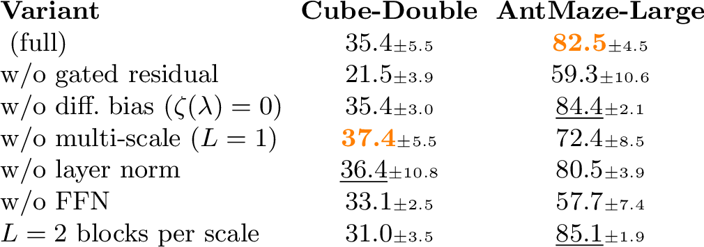
¿tbl:tab:ablation95components? reports the full component ablation. 5.4 discusses it. Two entries are not covered there. Removing the multi-scale extension costs \(10\) points on AntMaze-Large but slightly helps Cube-Double, and stacking two Dgca blocks per scale offers no benefit over one.
12.2 Sensitivity Analyses↩︎
[tbl:tab:sensitivities] sweeps three parameters on Cube-Double. 5.4 discusses the gate initialization. The token count has no effect across the tested range, which is consistent with fine spatial decomposition not driving the manipulation behavior. The head count declines mildly, and \(H = 1\) exceeds our default \(H = 4\). We retain \(H = 4\), because the configuration is held fixed across all twenty tasks and tuning it on the one task where the module underperforms would be the wrong trade. Our reported numbers therefore understate what per-task tuning would attain.
12.3 Where the Module Looks: Attention and Gate Analysis↩︎


Figure 5: Attention versus difference map on four Cube-Double samples. Each panel shows three rows (token counts \(T \in \{16, 4, 8\}\)), with \(\Delta\) in the first column (left bars), standard CA attention in the middle, and Dgca attention on the right. Both CA and Dgca place near-all attention mass on a single token. Dgca chooses a different token than CA on every sample, but neither systematically aligns with the argmax of \(\Delta\). On this manipulation task, attention concentration is sharp, but the choice of token is not driven by the difference map alone.. a — Sample 0, b — Sample 1, c — Sample 2, d — Sample 3

5 compares the attention distributions of standard cross-attention and Dgca on four Cube-Double samples against the corresponding difference maps. Both are nearly one-hot. Dgca attends to a different token than cross-attention on every sample, so the bias does shift the attended position, yet neither method selects the argmax of \(\Delta\). On this task the difference map therefore acts as a soft regularizer that displaces the head from the similarity-maximizing token, rather than as a literal pointer to the misaligned region.
6 plots the gate and \(\zeta(\lambda)\) trajectories that 5.4 discusses.
12.4 Why Visual-Puzzle Remains at Zero↩︎
| Method | Puzzle-3\(\times\)3 | Puzzle-4\(\times\)4 |
|---|---|---|
| Late Fusion (Dual) | 0 | 0 |
| Dual + CA | 0 | 0 |
| Dual + | 0 | 0 |
| Early Fusion (Orig) | 22 | 65 |
| HIQL [27] | 73 | 60 |
6 supports the encoder-level account in 5.4. Two remedies would apply. Cross-attention inside the CNN [66] preserves the correspondence that pooling destroys, and hierarchical planning sidesteps the requirement for it. Both are complementary to Dagr, since they act upstream of \(\phi\).
12.5 Computational Overhead↩︎
MS-Dgca roughly doubles per-step training time on Cube-Double and adds about 55% on Visual-Cube-Double, with a similar relative increase at inference time. The absolute budget remains practical. Detailed timings are in 11.
12.6 Per-Task Learned \(\zeta(\lambda)\)↩︎
| Task | Average \(\zeta(\lambda)\) |
|---|---|
| Navigation (AntMaze-Large) | 0.0066 |
| Single-Object Manipulation (Cube-Single) | 0.0227 |
| Multi-Object Manipulation (Cube-Double) | 0.0066 |
| Scene Arrangement | 0.0592 |
| Visual Navigation (Visual-AntMaze-Large) | 0.0074 |
| Visual Manipulation (Visual-Cube-Double) | 0.0069 |
The learned \(\zeta(\lambda)\) values stay at or barely above initialization on five of six tasks, with the only substantial deviation on Scene. The naive reading that manipulation needs more difference bias than navigation is not supported: AntMaze-Large and Cube-Double share essentially the same value. This is consistent with the component ablation result that removing the difference bias does not eliminate the navigation gains. Practically, the role of \(\Delta\) in MS-Dgca is best read as a structured inductive bias on the cross-attention scoring at initialization rather than as a heavily optimized contribution at convergence.
12.7 Per-Task Fusion Weights↩︎
| Task | Fine (\(T_1\)) | Medium (\(T_2\)) | Coarse (\(T_3\)) |
|---|---|---|---|
| Navigation (AntMaze-Large) | 0.360 | 0.257 | 0.383 |
| Single-Object Manipulation (Cube-Single) | 0.423 | 0.216 | 0.361 |
| Multi-Object Manipulation (Cube-Double) | 0.317 | 0.312 | 0.371 |
| Scene Arrangement | 0.224 | 0.144 | 0.632 |
| Visual Navigation (Visual-AntMaze-Large) | 0.683 | 0.137 | 0.180 |
| Visual Manipulation (Visual-Cube-Double) | 0.374 | 0.328 | 0.299 |
Fusion weights tell a less clean story than the design intuition in 4.3 alone would suggest. Scene drifts strongly toward the coarse scale, Visual Navigation toward the fine scale, and the remaining tasks stay close to uniform. We take this as evidence that the optimal analysis granularity is genuinely data-driven and that the role of the multi-scale architecture is to let the model select rather than to enforce a particular bias.
12.8 Gate and \(\lambda\) Evolution on Additional Tasks↩︎


12.9 Learning Curves↩︎


9 10 show the full training trajectories on the state-based and visual OGBench suites. The two views tell consistent stories, and together they sharpen the picture from the aggregate tables.
On the state-based suite (9), the navigation panels share a clear shape. Dagr departs from the two baselines early, typically within the first fifth of training, and the gap widens or stabilizes rather than closing. The most pronounced separation occurs on HumanoidMaze-large, AntMaze-large, and AntSoccer-arena, where the Dual baseline plateaus low and Dagr continues to climb. Standard CA tracks Dual closely on most navigation tasks, sometimes with a modest lift. Introducing a state-goal interaction is therefore not sufficient on its own. What separates Dagr from CA is the gated residual, as ¿tbl:tab:ablation95components? shows, and the curves confirm that the separation opens from the very first evaluation rather than emerging late. On PointMaze-medium and PointMaze-large the state space is small enough that the late-fusion bottleneck does not bite, and all three methods converge to similar curves. The manipulation panels (Cube-Single, Cube-Double, Scene) show no consistent ordering among the three methods, with curves overlapping inside the confidence band. This matches the aggregate table and is now shown to be stable across training rather than an artifact of the final checkpoint. The puzzle panels (Puzzle-3x3, Puzzle-4x4) stay flat near zero for all three methods throughout training, with no sign of a late breakthrough. We attribute this outcome to encoder-level rather than representation-level limitations in 12.4.
On the visual suite (10), the navigation behavior of 9 reproduces: on both Visual-AntMaze variants, Dagr pulls away from Dual and CA within the first quarter of training and the separation persists to the end. Visual manipulation curves cluster tightly, with no clear separation in either direction across the three methods, again consistent with the aggregate result. Visual-Puzzle remains at zero throughout training for every method, which is the strongest evidence we have that the bottleneck on these tasks is not something a goal-representation refinement, however structured, can fix.
Two cross-cutting observations emerge from comparing the two figures. First, the gains from Dagr appear early and grow with training rather than emerging only at convergence. This is consistent with the gated-residual design that opens slowly. As the gates lift and \(B\) in 3 grows, the value approximation gains room to improve when the state-conditioned signal actually helps. Second, where Dagr does not improve over Dual the behavior splits into two regimes. On the navigation tasks with small state spaces the three curves overlap. On Cube-Double and Scene Dagr settles below Dual from early in training and stays there, which rules out a late-stage optimization artifact and points at the architectural cause identified in 6.
References↩︎
Corresponding author.↩︎
Throughout the paper, \(\phi(g\mid s)\) denotes a deterministic function \(\phi:\mathcal{G}\times\mathcal{S}\to\mathbb{R}^d\), with the vertical bar reading “\(\phi\) of \(g\), parameterized by \(s\).” This is a notational convention and should not be read as a conditional distribution.↩︎