ML-Based Channel Quality Prediction
for URLLC Services of Connected Vehicles
July 15, 2026
Abstract
Connected and automated vehicles (CAVs) are expected to increasingly rely on 5G and future 6G ultra-reliable and low-latency communication (URLLC) services to support safety-critical and time-sensitive applications. Since wireless link conditions can vary rapidly in urban vehicular environments, proactively adapting service parameters based on future channel conditions is essential to maintain service continuity and reliability. In this paper, we investigate the use of machine learning (ML) techniques for channel quality prediction in vehicular URLLC scenarios. Specifically, we evaluate deep neural network (DNN) and long short-term memory (LSTM) models to forecast future channel conditions and enable proactive service adaptation with minimized performance degradation. The analysis is conducted using realistic simulations combining the SUMO traffic simulator and the Sionna-RT ray-tracing framework in a real urban environment reconstructed from OpenStreetMap data. Results show that ML-based prediction significantly outperforms approaches relying solely on past channel measurements and achieves performance close to the ideal case in which future channel conditions are perfectly known in advance. These findings demonstrate the potential of ML-driven prediction techniques to enhance the reliability and robustness of URLLC services for connected vehicular systems.
3cm(17cm,1cm) (Special Session)
1 Introduction↩︎
For conventional vehicles driven by humans, the best path to reach a destination is either the fastest one or the shortest one. When considering a CAV, whose safety and comfort significantly rely on the quality of the network connectivity assisting the driving to enhance its perception of the surrounding environment, other options may be preferred. Indeed, as detailed by the 5GAA in [1], it is envisioned that future CAVs will exploit a service called infrastructure-assisted environment perception to improve awareness of the surroundings and control movements; in such a service, the vehicle continuously receives environmental updates collected by other vehicles or by sensors installed along the roads. In addition to static and dynamic objects, trajectories and actuation commands need to be transmitted. This service requires a large throughput in DL, from a few hundreds kbps to more than 80 Mbps [1], [2]. If the required throughput is not available, then the amount of deliveredinformation decreases, violating the strict SLA required for safe autonomous navigation.
To model the interplay between network performance and vehicular automation, we leverage the concept of CAD Modes [3]. CAD Mode 0 indicates that the CAV relies solely on its onboard sensors. Higher CAD Modes are enabled when high throughput conditions are experienced, supporting advanced automated maneuvers.
Because wireless link conditions can vary rapidly in dynamic urban vehicular environments, proactively adapting service parameters based on future channel conditions is essential to maintain service continuity and reliability [4]. To navigate these rapid fluctuations, the network must rely on continuously accurate short-term prediction of the channel to determine the most suited CAD Mode and to satisfy the associated SLA. In this framework, ML-driven techniques become helpful in enhancing the communication with respect to non-ML procedures. To address this challenge, this work evaluates data-driven architectures, specifically DNN and LSTM models, in forecasting short-term link quality. We demonstrate that these ML models provide significantly more robust short-term channel estimation compared to reactive baselines, effectively safeguarding the stringent latency and reliability budgets demanded by URLLC applications. The main contributions of this paper are summarized as follows:
We propose a short-term channel quality estimation framework utilizing DNN and LSTM architectures to enable proactive URLLC service adaptation for connected and automated vehicles.
We evaluate our framework using a highly realistic ray-tracing-backed vehicular simulation combining SUMO [5] and Sionna-RT [6] modeled on a real-world urban area in Bologna.
Through extensive benchmarks, we demonstrate that the proposed ML approaches achieve robust reliability, reducing global SLA failure rates close to the perfect-channel-knowledge bound.
Time-series forecasting models, particularly LSTMs, have also been utilized to capture temporal dependencies and anticipate sudden throughput drops [10], [11]. In V2I environments, LSTMs have successfully been employed as network filter processes to predict channel conditions for optimal radio access technology (RAT) selection, significantly reducing queue backlogs [12]. Furthermore, recent advancements have benchmarked RNNs directly against classical Wiener filters for 2D-channel estimation in highly time- and frequency-selective V2X conditions, proving that data-driven equalizers exhibit superior resilience against Doppler spread and system parameter mismatches [13].
Looking toward future 6G deployments, the state-of-the-art is shifting toward integrating spatial-frequency ML-based channel estimation [14] and multimodal collaborative perception frameworks [15]. However, most existing works focus predominantly on uplink channels, static environments, or single-metric predictions. This paper extends the state-of-the-art by applying predictive DNN and LSTM architectures to highly dynamic urban vehicular DL communications, evaluating their impact directly on SLA failure rates and proactive QoS adaptation.
3 System Model↩︎
We assume a multi-cell scenario where the target CAV moves towards a certain destination while supported by an infrastructure-assisted environment perception service. Depending on the available resources, the level of service changes, following the concept of CAD Modes with corresponding SLA [3]. The highest CAD Modes allow the CAV to receive more information and therefore to drive with a longer perception horizon and with higher safety levels. Since the service is of type URLLC, only small delays and virtually no losses are tolerable.
Given this target service, the network needs to allocate the radio resources to the CAV with the highest possible CAD Mode that is compatible with the corresponding SLA and the radio link conditions. Thus, a reliable channel estimation is of paramount importance to ensure that the service requirements are met. Assuming a dedicated network slice is available [16] and a low service penetration, this study focuses on a single CAV without inter-cell interference. These simplifying assumptions will be relaxed in future works.
3.1 Radio Access and Allocation↩︎
While moving, the CAV is connected to a given cell. The network allocates the resources in that cell and the service performs data transmission, followed by link-level retransmission in case of losses. We assume the infrastructure-assisted environment perception service to be hosted at the network edge, which implies that the delay and losses introduced outside the radio link are negligible.
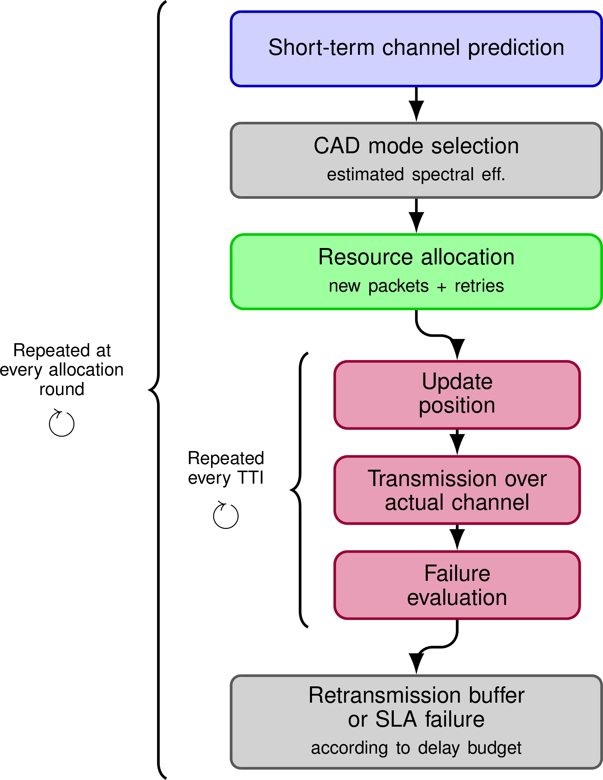
Focusing on the radio link, the allocation and transmission process is organized in ARs and TTIs, as represented in Fig. 1. The AR represents the granularity for radio resource allocation and includes a given number of TTIs, which in turn represent the granularity of the transmission. At the beginning of the AR, the channel quality is estimated (thus defining the MCS), the CAD Mode is selected, and the resources are allocated. Then, during each TTI the signal is transmitted in the allocated radio resources and the correctness of the reception is verified. For the sake of resource allocation, an estimation of the channel is needed, which we denote as \(\widehat{L}\). How to accurately estimate \(\widehat{L}\) is the subject of this work. Denoting the actual power loss by \(L_\text{actual}\), the objective of short-term channel estimation is to map a historical sequence of past power loss and contextual measurements \(\mathbf{x}\) spanning a past window of \(N\) TTIs to an estimated channel loss value \(\hat{L}(t)\): \[\hat{L}(t) = f\big(\{L_{actual}(t-1, \tau), \mathbf{x}(t-1, \tau)\}_{\tau=1}^{N}\big)\] where \(f(\cdot)\) represents the estimation framework (as detailed in Sec. 5).
Given \(\widehat{L}\), the network estimates the maximum throughput that it can support \(\widehat{T}_\text{DL, max}\), which is computed through the following equations: \[\widehat{\gamma}=\frac{P_\text{T} \, G_\text{T} \, G_\text{R}}{\widehat{L} \, P_\text{N}}=\frac{P_\text{T} \, G_\text{T} \, G_\text{R}}{\widehat{L} \, F_\text{R} \, k \, T_\text{0} \, B_\text{W}}, \label{eq:gamma}\tag{1}\] \[\widehat{\eta}=\alpha \, \log_2(1+\widehat{\gamma}), \label{eq:eta}\tag{2}\] \[\widehat{T}_\text{DL, max}=\widehat{\eta}_\text{max} \, B_\text{W}, \label{eq:throughput}\tag{3}\] where \(\widehat{\gamma}\) is the estimated SNR when assuming that all the bandwidth is used, \(P_\text{T}\) is the power transmitted before the BS antenna, \(G_\text{T}\) and \(G_\text{R}\) are the transmitting and receiving antenna gains, respectively, \(P_\text{N}\) is the noise power, \(F_\text{R}\) is the receiver noise figure, \(k\) is the Boltzmann constant, \(T_\text{0}\) is the reference temperature of 290 K, \(\widehat{\eta}\) is the estimated channel efficiency, and \(\alpha\) is a parameter that accounts for the protocol efficiency. To be noted that the channel efficiency corresponds in the real system to a certain MCS, with a lower MCS providing higher reliability at the cost of lower efficiency and viceversa. Therefore, \(\widehat{\eta}\) represents the maximum MCS that reliably guarantees \(\widehat{T}_\text{DL, max}\) if the SNR equals \(\widehat{\gamma}\). The maximum estimated throughput \(\widehat{T}_\text{DL, max}\) is then used to select the highest CAD Mode that can be supported. The latter is referred to as actual CAD Mode and its corresponding throughput is denoted as target throughput \(T^*_\text{DL}\) (with \(T^*_\text{DL}\leq\widehat{T}_\text{DL, max}\)).
Even if a single CAV and no inter-cell interference are considered, we schedule the minimum amount of resources required by the CAV to use the given CAD Mode. In particular, the network assumes the MCS corresponding to the channel efficiency \(\widehat{\eta}\) and allocates the bandwidth \(B_\text{actual}\leq B_\text{W}\) computed as: \[B_\text{actual} = T^*_\text{DL}/\widehat{\eta}\;.\]
3.2 Data Transmission and Retransmission↩︎
The maximum throughput \(\overline{T}_\text{DL}\) that can be supported without losses, assuming the allocated bandwidth \(B_\text{actual}\) and the actual channel conditions \(\gamma_\text{actual}\), can be derived as: \[\gamma_\text{actual}=\frac{P_\text{T} \, G_\text{T} \, G_\text{R}}{L_\text{actual} \, F_\text{R} \, k \, T_\text{0} \, B_\text{actual}}, \label{eq:gammaActual}\tag{4}\] \[\overline{T}_\text{DL}=\alpha B_\text{actual} \log_2(1+\gamma_\text{actual})\;.\]
If \(T^*_\text{DL}<\overline{T}_\text{DL}\), we assume no losses in the transmissions, otherwise part of the data needs retransmission. Specifically, we assume that the number of lost bits \(b_\text{err}\) needing retransmission equals: \[b_\text{err} = \begin{cases} 0 & \text{if } R_\text{DL} \leq \overline{T}_\text{DL} \\ ( T^*_\text{DL} - \overline{T}_\text{DL} ) \cdot T_\text{TTI} & \text{otherwise, } \end{cases}\] where \(T_\text{TTI}\) is the duration of the TTI. The bits \(b_\text{err}\) are buffered and retransmitted during the next AR with higher priority than the new data. The retransmitted bits that are not correctly received within the allowed maximum delay (or delay budget) are discarded, triggering an SLA failure event.
4 Case Study Scenario and Main Simulation Settings↩︎
The considered scenario is a portion of Bologna close to the Engineering Faculty. The road map was derived from the OpenStreetMap project [17]. The area, shown in Fig. 2, includes three distinct vehicular routes (namely Path 1, Path 2, and Path 3), each connecting the same origin and destination. Mobility patterns were generated in SUMO [5], considering road speed limits (up to 50 km/h) and free-flow traffic conditions. The three routes are comparable in length (between 2100 and 2400 m) and travel time (between 170 and 190 s).
Five tri-sector BSs (i.e., 15 cells) are located according to the real deployment as indicated in the LTEItaly database [18]. Each BS has antennas at a height of 25 m, with three cells oriented at 30°, 150°, and 270°, using single-element antennas with 3GPP TR 38.901 radiation patterns [19], as natively supported by Sionna RT. Vehicles are equipped with 1.5 m-high dipole antennas. Environmental features, such as building geometry and road layout, were imported from OpenStreetMap to enable accurate modeling. Concerning the online simulation, the adopted TTI is 0.5 ms and the AR is 5 ms. The maximum tolerated delay is set to 20 ms [20]. Regarding the handover mechanism, a combination of a dwell-time-based mechanism and an SNR threshold is implemented, where the handover is initiated if a neighboring cell’s SNR exceeds that of the serving cell by more than 3 dB and this condition persists for at least 1 s. From a service perspective, we assume three CAD Modes beyond zero, as detailed in Table 1.

| CAD Mode | DL throughput req. [Mbps] | |
|---|---|---|
| No requirement | No network-assisted perception; the CAV relies only on onboard sensors. | |
| \(1 < T_\text{DL} \leq 20\) | Basic network-assisted perception, suitable only for conservative automated operation. | |
| \(20 < T_\text{DL} \leq 50\) | Intermediate network-assisted perception, supporting automated operation with reduced confidence or tighter constraints. | |
| \(T_\text{DL} > 50\) | Extended and accurate network-assisted perception, enabling the highest supported automation level. |
5 Short-Term Channel Prediction↩︎
5.1 ML-Assisted Short-Term Channel Prediction Models↩︎
To achieve accurate short-term channel estimation, we benchmarked two distinct architectures: a feed-forward DNN and a recurrent LSTM network. Both architectures are trained to forecast imminent channel conditions based on the dataset generated via the Sionna RT and SUMO integration.
Dataset: Both models are trained on a set of engineered features derived from RSRP measurements and spectral efficiency experienced by a single vehicle traveling in our simulation framework over each of the 3 available paths of the case study scenario recalled in Section 4. Each sample of the dataset is composed of a series of consecutive RSRP values over the past \(N\) TTIs that are first min-max normalized. Then, the derivative, the minimum and the maximum values, the mean and the standard deviation in this interval are computed. The same is done for a series of \(N\) values of the spectral efficiency, which serves as contextual information. The size of the dataset is in the order of \(10^5\) samples. The training set is made from the samples related to Path 1 and Path 2 (i.e., about 66% of the total), while the test set is made from the samples related to Path 3 (i.e., about 33% of the total). These inputs provide both instantaneous and statistical context over a specific time window, allowing the network to potentially analyze trends and signal variability for better predictions.
DNN settings: The architecture chosen for the DNN is a fully connected MLP with three hidden layers, each containing 256 neurons. The learning rate is set to \(1\times 10^{-5}\), the mini-batch size is 64, and the model is trained for a single epoch.
LSTM settings: Regarding the LSTM model, it comprises 2 recurrent layers with 100 neurons each. The learning rate is set to \(1\times 10^{-5}\), the mini-batch size is 64, the number of epochs is 1. For both networks, the low number of epochs is justified by the dense size of the dataset, which facilitates rapid convergence.
Loss functions: To optimize the networks for URLLC constraints, we evaluate three distinct objective functions: MAE, MSE, and a custom asymmetric loss function (denoted as MAE+MSE), which applies standard MAE penalties for channel underestimations, but switches to an MSE penalty for channel overestimations. This asymmetric behavior strictly punishes optimistic channel predictions, which are catastrophic in URLLC settings because they lead to severe resource starvation, packet drops, and fatal retransmission loops.
Output: Both models aim to provide a specific, single-value prediction: the worst case RSRP in the next AR. Considering ARs of a length of 10 TTIs, this corresponds to predicting the worst case over the next 10 TTIs. This aims at determining the worst channel conditions in the AR in order to avoid and limit retransmissions. Starting from this prediction, the spectral efficiency and the achievable bit rate can be derived. We chose to predict the worst case in order to limit retransmissions and data loss and to have a system that is more forgiving with imprecise predictions. In fact, the dataset is subject to fast channel variations and predicting the best case or an average case would have led to a network that is more susceptible to noise and prone to make riskier predictions.
5.2 Benchmarks↩︎
The following schemes are considered as benchmarks for the proposed ML-based solutions.
Ideal channel knowledge in each TTI, where the scheduler knows in advance the exact channel in each TTI of the AR; this is used as an unrealistic upper-bound to the performance, indicated as “Ideal per TTI”;
Ideal channel knowledge of the worst case in the AR, where the scheduler knows in advance the channel of the worst TTI in the AR; this benchmark also sets the upper-bound which the scheduler should target with its estimation, and is indicated as “Ideal per AR”;
Estimation of the channel in the next AR equal to the mean of the last \(N\) TTIs; this scheme gives a benchmark of standard approaches based on the average past channel and is indicated as “Past average”;
Estimation of the channel in the next AR equal to the worst case of the last \(N\) TTIs; this scheme is a benchmark of non-ML solutions, where a conservative approach is used to cope with the URLLC requirements; this scheme is denoted as “Past minimum”.
These approaches set benchmarks with two ideal solutions (the first two items) and two history-based approaches. Given the URLLC requirements, a conservative approach needs to be used and therefore the main benchmarks are the “Ideal per AR” and “Past minimum”, while the other two are provided as references of what would be achieved neglecting the requirements.
5.3 Metrics of Interest↩︎
Results are derived in terms of the following metrics to quantify the effectiveness of the proposed short-term channel estimation:
CAD score: it measures the effectiveness in terms of the selected CAD Mode for the chosen path, calculated as: \[S =\sum_{m=0}^{M}w_m CAD_{m}^{\%}\;,\] where \(CAD_{m}^{\%}\) is the percentage of time spent in each CAD Mode, \(M\) is the number of CAD Modes, and \(w_m\) defines the weights that are set as \(w_0=0\), \(w_1=0.02\), \(w_2=0.4\), and \(w_3=1\) to capture the highest relevance of the higher CAD Modes. This setting is derived from the ratio between the throughput associated to the CAD Mode and the maximum achievable throughput. This ensures that the CAD score \(S\) varies between \(0\) and \(1\). In addition, this set choice allows to interpret \(S\) as the average throughput experienced by the CAV on the path, expressed as a percentage of the maximum achievable throughput. For instance, a path score of \(0\%\) and \(100\%\) corresponds to the limit cases where the CAV spends all the time either in CAD Mode 0 or in CAD Mode 3 (i.e., \(0\%\) and \(100\%\) of the maximum throughput on average).
SLA failure rate: it measures the portion of time when the agreed SLA is not satisfied, calculated as: \[\label{eq:Rsf} R_{sf}=\frac{T_{sf}}{T_{path}},\tag{5}\] where \(T_{sf}\) is the time during which the SLA is not satisfied, and \(T_{path}\) is the overall travel time; the SLA failure rate is given as an overall average or separately per each CAD Mode; in the latter case, both the numerator and denominator of 5 are restricted to the given CAD Mode, and this allows to assess the impact of failures that are associated to different safety risks.
6 Results↩︎
This section evaluates the performance of the proposed DNN and LSTM short-term predictors. Comprehensive performance metrics across all loss functions for structural benchmarks (\(N \in \{10, 50, 100\}\)) are presented in Table 2.
6.1 Channel Estimation using DNN↩︎
6.1.1 DNN with MAE↩︎
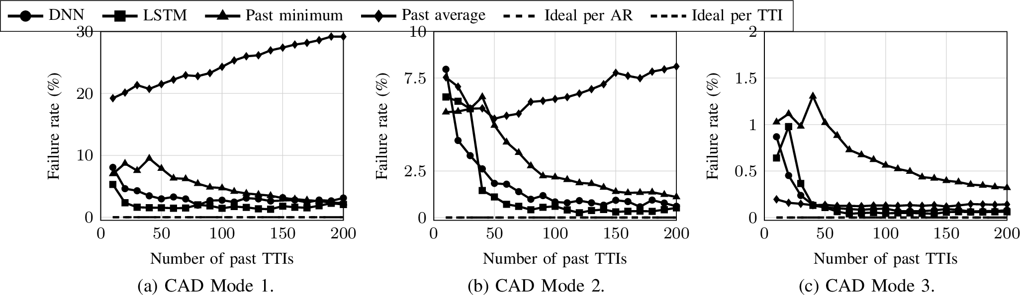
Figs. [fig:DNN-path-MAE] and [fig:DNN-tot-fail-MAE] report the CAD score (\(S\)), the total SLA failure rate (\(R_{sf}\)), and CAD-aggregated metrics against the past window size \(N\). While Ideal per TTI represents a theoretical performance bound under continuous feedback, Ideal per AR serves as the realistic optimization target for the scheduler. When considering history-based baselines, we can observe that Past average is too optimistic. It registers an inflated path score outperforming the Ideal per AR limit, but triggers severe SLA violations that scale monotonically with \(N\). The DNN stably tracks a score close to the Ideal per AR independently of \(N\) (Fig. [fig:DNN-path-MAE]), achieving an aggregated SLA failure rate below \(0.5\%\) for \(N \geq 50\) (Fig. [fig:DNN-tot-fail-MAE]). Specific CAD Mode configurations are detailed in Fig. 5. The baseline behaviors mirror the aggregated case, where expanded context penalizes the performance of Past minimum and escalates the risk profile of Past average. A notable exception is observed for CAD Mode 3, where the Past average is stable and below 0.2%, indicating that high-SNR conditions are inherently more resilient to variance and estimation mismatch. The DNN consistently outperforms the empirical baselines across all operating modes when \(N \geq 50\), hitting its optimal reliability bounds in CAD Mode 3.
6.1.2 DNN with MSE↩︎
Evaluating the MSE configuration in Table 2 reveals identical trends regarding context scaling; structural gains in reliability materialize sharply when moving from \(10\) to \(50\) TTIs, entering a saturation plateau at \(100\) TTIs. Comparing the the DNN-MSE framework to MAE estimates, we observe a slightly lower score (\(56.85\%\) vs. \(58.14\%\) at \(50\) TTIs). This behavior is due to the fact that the loss function now is harsher with respect to outliers and the network tends towards a more cautious behavior.
6.1.3 DNN with a Combination of MAE and MSE↩︎
The mixed asymmetric configuration (Table 2) explicitly punishes channel overestimations, which are critical catalysts for packet drops and URLLC retransmissions. This structural penalty induces a highly cautious behavior: at \(50\) TTIs, the path score decreases significantly (\(52.24\%\)), but yields the lowest overall DNN SLA failure rate (\(0.24\%\)), validating the intended design objective.


| Method | 10 TTIs | 50 TTIs | 100 TTIs | 10 TTIs | 50 TTIs | 100 TTIs |
| DNN (MAE) | ||||||
| DNN (MSE) | ||||||
| DNN (MAE+MSE) | ||||||
| LSTM (MAE) | ||||||
| LSTM (MSE) | ||||||
| LSTM (MAE+MSE) | ||||||
| Past minimum | ||||||
| Past average | ||||||
| Ideal per AR | ||||||
| Ideal per TTI |
6.2 Channel Estimation using LSTM↩︎
6.2.1 LSTM with MAE↩︎
As illustrated in the aggregated metrics of Fig. 5, the recurrent model tracks the Ideal per AR score closely across all values of \(N\), though maintaining a slightly lower nominal profile than the DNN. Reliability convergence matches the feed-forward model, securing an SLA failure rate below \(0.5\%\) when \(N \geq 50\).
At the individual mode level (Fig. 5), the LSTM reveals distinct performance advantages over the DNN when \(N \geq 50\). The minimum recorded failure rate drops from \(1.94\%\) to \(1.26\%\) in CAD Mode 1, from \(0.58\%\) to \(0.26\%\) in CAD Mode 2, and from \(0.065\%\) to \(0.039\%\) in CAD Mode 3. The net global minimum failure rate drops to \(0.19\%\) for the LSTM compared to \(0.21\%\) for the DNN. This incremental gain in safety margins stems from the sequential processing capability of the LSTM, though the architectural choice between the two models represents a direct trade-off between strict safety optimization and computational overhead.
6.2.2 LSTM with MSE and Mixed Asymmetric Losses↩︎
As shown in Table 2, the LSTM-MSE model displays tracking patterns close to its MAE baseline. However, when executing under the asymmetric MAE+MSE loss, the LSTM delivers the most robust metrics of the study: at \(100\) TTIs, it reduces the global SLA failure rate to an absolute low of \(0.13\%\), proving highly responsive to overestimation penalties.
6.3 Main Findings on the Short-Term Channel Prediction↩︎
The conducted study provides several insights about the behavior of the covered solutions. For what concerns the short-term channel prediction based only on the history, the following main considerations hold:
Past average provides the highest score among the non-ideal predictions, but the highest SLA failure rate. The larger the number of the past TTIs (\(N\)), the larger the SLA failure rate, the lower the path score.
Past minimum reduces the SLA failure rate as the number of past TTIs (\(N\)) increases, but significantly reduces the path score, while a larger \(N\) improves it.
For ML-based short-term channel prediction, the main findings are as follows:
With DNN, the score only slightly decreases as the number of considered TTIs \(N\) increases.
After 50 past TTIs, the SLA failure rate converges, and the best performance is achieved.
An SLA failure rate equal to 0 is not achieved.
No remarkable differences are observed with different models (DNN or LSTM) or loss functions (MAE, MSE, and combination of MAE and MSE).
The results are overall very promising and require further validation. The DNN appears sufficient with the current modeling, and future work should be dedicated to improve such modeling and to investigate if the approach applies when changing the scenario and environmental conditions.
7 Conclusion and Future Work↩︎
In this paper, we introduced an ML-driven methodology for proactive URLLC service adaptation in 5G/6G connected vehicular networks. By utilizing accurate channel datasets generated via Sionna-RT and SUMO in a realistic urban topology, we tested the ability of DNN and LSTM architectures to forecast short-term channel degradation. The results confirm that ML-based prediction models significantly outperform standard history-based conservative short-term channel estimation. Specifically, considered ML models utilizing a custom asymmetric MAE/MSE loss function effectively restricts SLA failure rates to strictly bounded URLLC margins while maintaining an operational path score close to the ideal, perfect-knowledge upper bound. Future work will target scenarios with multiple vehicles and interference to assess to which extent the prediction can be affected.
Acknowledgment↩︎
This work has been conducted in the framework of the CNIT-WiLab and the WiLab-Huawei Joint Innovation Center.
References↩︎
©2026 IEEE. Personal use of this material is permitted. Permission from IEEE must be obtained for all other uses, in any current or future media, including reprinting/republishing this material for advertising or promotional purposes, creating new collective works, for resale or redistribution to servers or lists, or reuse of any copyrighted component of this work in other works.↩︎