Microstructure-Conditioned Surrogate Models for Graded Multiscale Optimization of Mycelium Composites
July 15, 2026
Abstract
Emerging sustainable materials increasingly rely on engineered hierarchy and microstructure to achieve control of their properties and mechanical behavior. Optimizing these materials with controllable microstructures requires efficient multiscale simulations. Data-driven surrogate models for the microscale can accelerate multiscale simulations, but require large amounts of data even for a fixed microstructure. When a range of microstructures is considered, as is the case in multiscale optimization, even more data is needed to train a surrogate. To overcome this challenge, we condition a hybrid physics-data surrogate on microstructural variables using a hypernetwork. This approach enables accurate predictions of multiscale mechanical behavior for a mycelium-woodchip composite material, even when trained on small datasets. The conditioned surrogate makes multiscale simulations of functionally graded structures tractable, and we validate it against a full FE\(^\mathrm{2}\) simulation. We optimize a graded multiscale disk, and reduce the peak stress by 42% compared to one with a random microstructure. Then, we go one step further, conditioning the network directly on manufacturing variables that can have a complex influence on the microstructure. This is a practical route to engineer the microscale for desired macroscale behavior. This contribution highlights the benefits of microarchitectured structures and demonstrates how conditioned surrogate models enable their multiscale optimization, which will accelerate the development and design of future sustainable materials and structures.
Multiscale ,Machine learning ,Optimization ,Mycelium-woodchip composite
1 Introduction↩︎
Homogeneous structural materials are widespread due to their uniformity and ease of manufacturing. However, in nature, many heterogeneous materials evolved, such as bones, teeth, wood, and bamboo, as these are more mechanically efficient designs [1]. These are examples of functionally graded materials, characterized by having continuous spatial variation of material properties at the macroscale. Precisely manufacturing a functionally graded material similarly enables the design of more efficient structures. However, optimizing such a grading requires relating the local microstructure to the macroscopic response.
FE\(^\mathrm{2}\) is a concurrent approach to simulate both scales, where microscale representative volume elements (RVEs) are embedded in a macroscale domain. Solving a separate boundary value problem for every quadrature point makes this very computationally demanding. Instead, data-driven models can act as surrogates for the microscale simulations, estimating the homogenized microscale response at a fraction of the computational costs. Many surrogates have been developed, both purely data-driven and based on physical principles, capturing the behavior in materials ranging from hyperelasticity and viscoelasticity to plasticity, damage, and fracture [2]. For elastic materials, data-driven approaches have enabled multiscale graded optimization by predicting an effective elasticity tensor from the microstructure [3]–[5]. For nonlinear materials, however, surrogates are typically trained to map strains to homogenized stresses for a single, fixed microstructure, and therefore cannot account for varying underlying microstructures. This makes them unsuitable for simulating functionally graded composites, where the microstructure varies across the domain.
One way of overcoming this limitation is by using a surrogate model that takes the complete microstructure as input, for example, using a convolutional neural network (CNN) [6], [7] or a graph neural network (GNN) [8]. Microstructural geometric variables can also be used to directly predict the effective properties of the material [9]. Alternatively, they can be directly passed as additional inputs, for example to the hidden state in a gated recurrent unit [10], or encoded into a small vector before concatenating it to the hidden embedding in a network [11]. These approaches have the potential to be used in the optimization of a graded material, but generally still require vast amounts of training data. Meta-learning or transfer learning can adapt or fine-tune a base model to limited new data from a different underlying distribution [12]–[15], but still require separate data collection for each new setting, making it infeasible for continuous gradings.
An effective approach to reducing the required amount of training data in surrogates is to incorporate a physical bias in the model. Physically Recurrent Neural Networks (PRNNs) have recently shown a remarkable ability to learn based on tiny datasets, overcoming the bottleneck of costly data generation [16]. As the microscale constitutive models are embedded directly inside the PRNN architecture, their material properties can be modified directly without requiring retraining or additional data collection [17]. This essentially conditions on material parameters without having to train with more than one parameter value. In a similar vein, a Deep Material Network (DMN) learns the homogenization behavior of a multi-phase material [18], while maintaining the microscale material models. DMNs have recently been conditioned on the microstructure, such as by interpolating between several DMNs trained on different RVEs, by conditioning on the volume fraction [19], and by conditioning on a latent space learned from the microscale geometry [20]. Since a DMN essentially learns the homogenization scheme, this conditioning can only be done by modifying the weights of the network. The weights of the DMN are thus predicted by a separate neural network; such a second network is generally called a hypernetwork. HyperCANs follow the same principle, where, based on the geometry of a unit cell truss lattice, a hypernetwork learns the weight parameters of an input convex neural network that predicts the strain energy density given a deformation gradient [21].
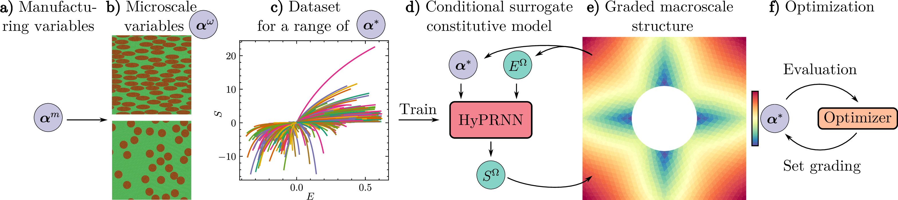
In this work, we opt for PRNNs because they can already account for variations in the microscale material properties, and extend them to be conditioned on microstructural variables using a hypernetwork, which we refer to as a HyPRNN. A schematic overview of the methods in this work is presented in Figure 1. Our contributions are as follows:
Conditioning a PRNN on microstructural variables. While traditional PRNNs can already account for differences in microstructural material properties, they cannot account for geometric variations in the microstructure. We enable this using a hypernetwork that learns the PRNN weights based on the microstructural variables.
PRNNs for geometric nonlinearity in finite strains. To capture geometrically nonlinear effects, we introduce a more flexible nonlinear PRNN encoder. In addition, we modify the previously used linear encoder to remain valid for large deformations.
Demonstration of a tractable multiscale optimization. With the HyPRNN, we iteratively run a graded multiscale simulation inside an optimization algorithm to find a grading that leads to better mechanical performance.
Conditioning on manufacturing variables. When the microstructure exhibits a complex geometry that cannot be parametrized explicitly, a common strategy is to condition on a black-box latent space learned by a generative model that captures its properties [20]. We introduce a new approach that instead conditions directly on the manufacturing variables generating the microstructure, eliminating the need for such an additional model. This approach is demonstrated by conditioning on the inputs of a discrete-element method simulation that creates the microscopic geometry.
2 Inspiration: mycelium-woodchip composites↩︎
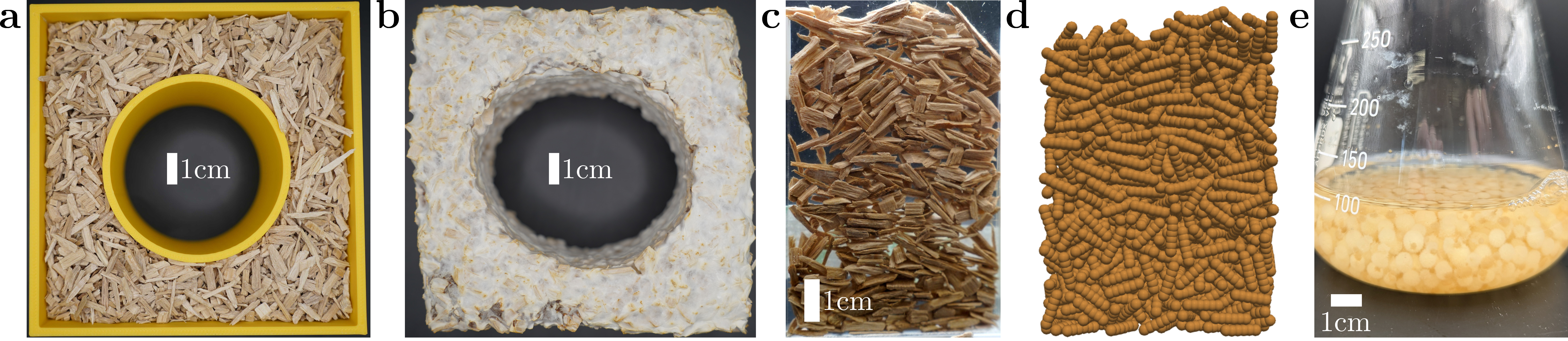
While this work focuses on computational methods, we base our requirements on applications such as functionally graded bio-based composites. In particular, we are interested in mycelium-woodchip composites, which are actively researched for the construction, packaging, and insulation industries [22], and benefit from microscale structure. Mycelium is considered the vegetative root-like structure of fungi and is composed of hyphae, which are tube-like fibers with a diameter of about 1 [\(\mu\)m]. Growing on a substrate of woodchips or natural fibers, it acts as a binder that forms a lightweight yet stiff biodegradable composite [23], [24]. For instance, Figure 2a-b shows woodchips in a mold, to which inoculated water is added, forming a mycelium-bound composite. As an engineered living material, its unique properties include the ability to grow and self-repair [25], [26], and has been explored for mechanical use [23], [27]. Controlling the substrate properties and mycelium growth can tailor a functionally graded material to specific macroscale behavior.
Modeling this macroscale behavior requires the mechanical properties of the individual constituents. Mechanical tests on pure mycelium by Islam et al. revealed that its Young’s modulus depends on the density, giving an average of \(E\) = 1.3 [MPa] for a density of 34 [kg/m\(^3\)], and Poisson’s ratio \(\nu\) = 0.275 [-] (Lamé parameters \(\lambda\) = 0.62 [MPa], \(\mu\) = 0.51 [MPa]) [28]–[30]. We adopt these properties and, motivated by their density dependence, also consider a variation in \(\mu\). Mycelium is often characterized similarly to foam, and its constitutive behavior is commonly modeled using a hyperelastic material model [22], [29], [30]. For the woodchips, isotropy and standard beech properties are assumed, with \(E\) = 13000 [MPa] and \(\nu\) = 0.375 [-].
Various aspects of the manufacturing process of a mycelium-woodchip composite are shown in Figure 2. Woodchips are inoculated with mycelium spores and placed in formwork, where the mycelium grows over the span of a few weeks to create the composite material. The growth depends on many factors, such as available nutrients, water content, and air. A graded material can be formed by, for example, controlling the distribution of both woodchips and pellets. Figure 2c,e shows these constituents, and Figure 2d shows the result of numerically simulating the woodchip deposition process. Experimentally finding the optimal grading of woodchip distribution and angle is not feasible, and even numerically this remains challenging.
3 Finite strain mechanics↩︎
This section briefly introduces the computational methods and notations associated with finite strain continuum mechanics and hyperelasticity. For a reference point \(\mathbf{X}\) in the initial configuration of a body undergoing deformation, we can define a function \(\boldsymbol{\varphi}\) that maps the point to an updated configuration \(\mathbf{x}=\boldsymbol{\varphi}(\mathbf{X},t)\) at time \(t\). The deformation gradient of the material follows as \[\mathbf{F} = \frac{\partial \boldsymbol{\varphi}}{\partial \mathbf{X}}, \quad \text{with} \quad J=\det \mathbf{F} > 0.\] Commonly used deformation tensors are the Cauchy-Green tensor (\(\mathbf{C}\)) and the Green-Lagrange strain (\(\mathbf{E}\)): \[\mathbf{C}=\mathbf{F}^T\mathbf{F}, \qquad \mathbf{E}=\dfrac{1}{2}(\mathbf{C}-\mathbf{I}).\] A hyperelastic solid derives stress from a stored energy density \(W=W(\mathbf{F})\). The stress measures are computed as \[\mathbf{P}=\frac{\partial W}{\partial \mathbf{F}}, \qquad \mathbf{S}=2\,\frac{\partial W}{\partial \mathbf{C}}, \qquad \mathbf{S}=\mathbf{F}^{-1}\mathbf{P},\] where \(\mathbf{P}\) is the first and \(\mathbf{S}\) the second Piola–Kirchhoff stress tensor. \(\mathbf{C}\), \(\mathbf{E}\), and \(\mathbf{S}\) are symmetric tensors. We employ a simple hyperelastic material model in this work, following a compressible neo-Hookean formulation. With Lamé parameters \(\mu\) and \(\lambda\), its energy in 3D is defined as: \[W(\mathbf{F})=\frac{\mu}{2}\,(I_1-3)\;-\;\mu\,\ln J\;+\;\frac{\lambda}{2}\,(\ln J)^2, \quad I_1=\mathrm{tr}(\mathbf{C}).\] The second Piola-Kirchhoff stress then follows as \[\mathbf{S}=\mu\,(\mathbf{I}-{\mathbf{C}}^{-1})\;+\;\lambda\,\ln J\;{\mathbf{C}}^{-1}.\]
In a two-scale setting (FE\(^\mathrm{2}\)), the macroscopic problem on domain \(\Omega\) provides the macroscopic deformation gradient \(\mathbf{F}^{\Omega}\) to an RVE that resolves equilibrium in the microscale domain \(\omega\). The microscale problem returns the homogenized stress as a volume average: \[\mathbf{P}^{\Omega} = \dfrac{1}{|\omega|} \int_{\omega} \mathbf{P}^{\omega}\, d\omega.\]
4 Microstructure-conditioned PRNNs↩︎
4.1 PRNNs for finite strain↩︎
In this work we will use PRNNs as a surrogate for the microscale model, building on earlier work that demonstrated that PRNNs perform well in a finite strain framework [31]. The PRNN consists in an encoder - material - decoder framework, with operations that conceptually mirror computational homogenization in an RVE. The encoder learns to compute microscopic strain quantities from the macroscopic strain input. These microscopic strains are passed through a set of fictitious material points employing physics-based microscopic material models to produce microscopic stresses. These material models are the same ones also used as constitutive equations in the RVE for data generation, in this case neo-Hookean. The decoder then combines the microscopic stresses into a macroscopic stress. The general flow of the PRNN used in this work is thus as follows:
\[\mathbf{F}^{\Omega} \;\rightarrow\; \mathbf{E}^{\Omega} \underbrace{\;\rightarrow\; \hat{\mathbf{E}}^{\omega}_{m_1,\dots,M} }_{\text{encoder}} \underbrace{\;\rightarrow\; \hat{\mathbf{S}}^{\omega}_{m_1,\dots,M}}_{\text{material model}} \underbrace{\;\rightarrow\; \hat{\mathbf{S}}^{\Omega} \vphantom{\hat{\mathbf{C}}^{\omega}_{m_1,\dots,M}}}_{\text{decoder}} \;\rightarrow\; \hat{\mathbf{P}}^{\Omega}.\] Here, \(M\) is a hyperparameter that corresponds to the number of fictitious material points used.
In the small-strain plasticity setting that inspired the original PRNN [16], most of the nonlinearity comes from the material behavior, which is captured by the material model present in the network. In our finite-strain hyperelastic model, a significant amount of additional geometric nonlinearity can occur. With the material model capturing material nonlinearity, and the decoder mirroring the homogenization step, the encoder is the natural place for capturing geometric effects. We therefore explore a nonlinear encoder with increased flexibility in addition to a linear encoder.
There are two conditions we want the encoder to satisfy. First, in the undeformed state, we want all microscopic strains to vanish: \(\mathbf{F}^{\Omega}=\mathbf{I} \to \hat{\mathbf{E}}^{\omega}_m = \mathbf{0}\). This causes all microscopic stresses to remain zero, leading to a zero predicted stress. Second, to be able to compute the response of the fictitious material points, which are given by a classical neo-Hookean model, the encoder must output valid deformation tensors. For this neo-Hookean model, this means ensuring that \(\hat{\mathbf{C}}^{\omega}_m\) is positive definite.
4.1.1 Linear encoder↩︎
For each fictitious material point, a corresponding weight matrix \(\mathbf{W}^E_m\) is learned that computes the microscopic strain: \[\hat{\mathbf{E}}^{\omega}_m = \mathbf{E}^{\Omega}\,\mathbf{W}^E_m.\] We use \(\mathbf{E}^{\Omega}\) as input instead of \(\mathbf{F}^{\Omega}\), as it helps satisfy the first condition. Because \(\mathbf{E}^{\Omega}\) is zero in the undeformed state, \(\hat{\mathbf{E}}^{\omega}_m\) will be zero too, regardless of \(\mathbf{W}^E_m\).
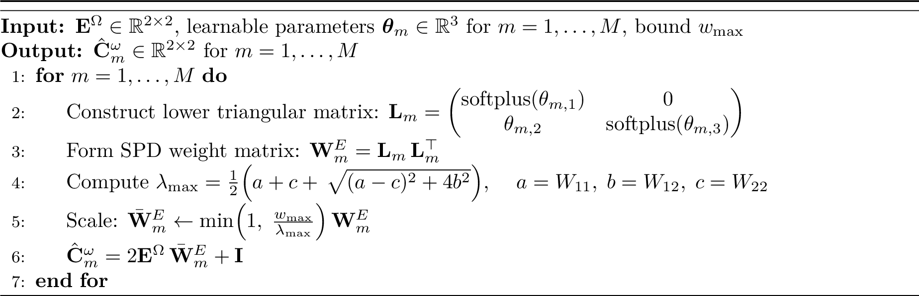
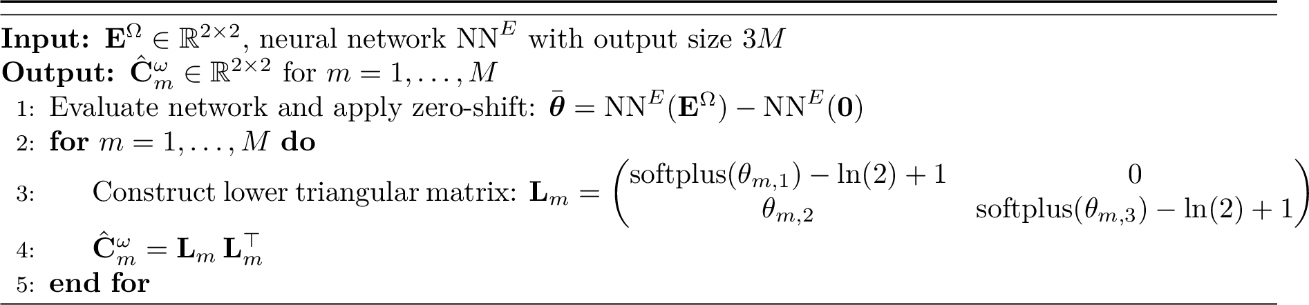
Satisfying the second condition is more challenging. The \(\hat{\mathbf{C}}^{\omega}_m\) used by the fictitious material model is computed as: \[\hat{\mathbf{C}}^{\omega}_m = 2 \hat{\mathbf{E}}^{\omega}_m + \mathbf{I} = 2 (\mathbf{E}^{\Omega}\,\mathbf{W}^E_m) + \mathbf{I},\] where \(\mathbf{E}^{\Omega} = \frac{1}{2}(\mathbf{F}^\top\mathbf{F} - \mathbf{I})\) is symmetric by definition. First, we construct \(\mathbf{W}^E_m\) to be positive definite by using a Cholesky-based parametrization: \[\mathbf{W}^E_m = \mathbf{L}_m\mathbf{L}_m^\top \succ 0, \;\; \mathbf{L}_m = \begin{bmatrix} \text{softplus}(\theta_{m,1}) & 0 \\ \theta_{m,2} & \text{softplus}(\theta_{m,3}) \end{bmatrix}.\] In 2D equilibrium, \(\hat{\mathbf{C}}^{\omega}_m\) is [\(2\times2\)], and the encoder thus has \(3M\) learnable parameters we gather in a vector \(\boldsymbol{\theta}\). Since the eigenvalues of the weight matrix \(\lambda_{(\mathbf{W}^E_m)}\) are strictly positive, the minimum eigenvalue is: \[\lambda_{\min(\hat{\mathbf{E}}^{\omega}_m)} = \lambda_{\min(\mathbf{E}^{\Omega}\mathbf{W}^E_m)} \geq \lambda_{\min(\mathbf{E}^{\Omega})} \cdot \lambda_{\max(\mathbf{W}^E_m)}.\] The eigenvalues of \(\mathbf{F}^{\Omega}\) are positive by definition, since they will come from the macroscale solution field, leading to \(\lambda_{\min(\mathbf{F}^{\Omega})} > 0\), and therefore the minimum eigenvalue of \(\mathbf{E}^{\Omega}\) is: \[\lambda_{\min(\mathbf{E}^{\Omega})} = \min_i \frac{\lambda_{(\mathbf{F}^{\Omega})}^2 - 1}{2} > -\frac{1}{2}.\] The minimum eigenvalue of \(\hat{\mathbf{C}}^{\omega}_m\) is thus: \[\lambda_{\min(\hat{\mathbf{C}}^{\omega}_m)} = 2 \lambda_{\min(\hat{\mathbf{E}}^{\omega}_m)} + 1 = 2 \lambda_{\min(\mathbf{E}^{\Omega})} \lambda_{\max(\mathbf{W}^E_m)} + 1 = - \lambda_{\max(\mathbf{W}^E_m)} + 1.\] This gives us the following criterion: \[\lambda_{\max(\mathbf{W}^E_m)} \leq 1 \implies \det(\hat{\mathbf{C}}^{\omega}_m) > 0 \quad \forall\, \mathbf{F}^{\Omega}: \det(\mathbf{F}^{\Omega}) > 0.\] We enforce this by scaling \(\mathbf{W}^E_m\) when its eigenvalues exceed this limit: \[\bar{\mathbf{W}}^E_{m} = \mathbf{W}^E_m \cdot \min\!\left(1,\; \frac{1}{\lambda_{\max(\mathbf{W}^E_m)}}\right).\] While this guarantees a valid \(\hat{\mathbf{C}}^{\omega}\) for any \(\mathbf{F}^{\Omega}\), it limits the flexibility of the encoder. If the range of macroscopic deformation gradients is known, this constraint can be relaxed: \[\bar{\mathbf{W}}^E_{m} = \mathbf{W}^E_m \cdot \min\!\left(1,\; \frac{w_{\max}}{\lambda_{\max(\mathbf{W}^E_m)}}\right),\] where \(w_{\max}\) can be modified based on the expected deformations. For \(w_{\max}=1.25\), \(\hat{\mathbf{C}}^{\omega}_m\) is valid if \(\lambda_{\min(\mathbf{F})} > \sqrt{0.2} \approx 0.447\), meaning that one needs a compressive strain exceeding 55% to produce an invalid \(\hat{\mathbf{C}}^{\omega}_m\). An example implementation in 2D is presented in Algorithm 3. Note that during inference, \(\bar{\mathbf{W}}^E_m\) is fixed and can be stored and used directly.
4.1.2 Nonlinear encoder↩︎
There are several ways to design a nonlinear encoder variant, but we want it to satisfy the same two conditions outlined previously. The approach we take is to first allow arbitrary nonlinear operations on the inputs, and then constrain this intermediate state.
We use an arbitrary neural network, \(\mathrm{NN}^E\) that takes \(\mathbf{E}^{\Omega}\) as input and outputs \(3M\) variables (three local strain components per fictitious material point), gathered in \(\boldsymbol{\theta}\). Considering the first condition, we apply a zero-shift to ensure \(\boldsymbol{\theta}\) is zero in the undeformed state: \[\bar{\boldsymbol{\theta}} = \mathrm{NN}^E(\mathbf{E}^{\Omega}) - \mathrm{NN}^E(\boldsymbol{0}).\] Each \(\bar{\boldsymbol{\theta}}_m \in \mathbb{R}^3\) is then mapped to \(\hat{\mathbf{C}}^{\omega}_m\) through a Cholesky-style parametrization, \[\hat{\mathbf{C}}^{\omega}_m = \mathbf{L}_m \mathbf{L}_m^{\top}, \qquad \mathbf{L}_m = \begin{bmatrix} \sigma(\theta_{m,1}) & 0 \\ \theta_{m,2} & \sigma(\theta_{m,3}) \end{bmatrix},\] where \(\sigma(x) = \mathrm{softplus}(x) - \ln(2) + 1\) is a shifted softplus chosen so that \(\sigma(0)=1\). This ensures that when \(\bar{\boldsymbol{\theta}}_m\) is zero, \(\hat{\mathbf{C}}^{\omega}_m=\mathbf{I}\), satisfying the first condition. In addition, this matrix is positive definite by definition, and thus satisfies the second condition. In contrast to the linear encoder, where the Cholesky parametrization is used to construct the weights, here it directly creates \(\hat{\mathbf{C}}^{\omega}_m\).
4.1.3 Decoder↩︎
The decoder combines all predicted microscopic stress tensors into the macroscopic stress. Previous work on PRNNs for finite strains compared a dense and sparse decoder [31]. In the dense decoder, every microscopic stress component is densely connected to the macroscopic stress output. The sparse decoder, which we also adopt, combines the stresses in a component-wise manner instead: \[\mathbf{S}^{\Omega}_i = \sum_m \mathbf{S}^{\omega}_{m,i} \operatorname{softplus}(w_{m, i}).\] By analogy with volumetric homogenization, the weights here represent the volume (or area), and the softplus function ensures these are positive.
4.2 A hypernetwork-based PRNN↩︎
PRNNs cannot generally be conditioned on microstructural parameters. Different routes can be explored to still include them in the PRNN architecture. The straightforward approach to condition a data-driven model on additional parameters is by concatenating the variables as additional inputs. For the PRNN, this approach conflicts with the role of the encoder, which is meant to map only the macroscopic strain onto a latent representation of microscopic strains. While the nonlinear encoder could in theory support additional inputs, the linear encoder would require further modifications, and would not allow the decoder to adapt either.
Instead, we preserve the existing PRNN architecture, and use a hypernetwork \(\mathcal{H}\) that learns the PRNN encoder and decoder parameters based on microstructural variables. In effect, the hypernetwork learns a continuous mapping from microstructural variables to the space of PRNN weights, rather than producing a single set of weights tied to one microstructure. The encoder and decoder weights are learned by the same hypernetwork, and the only trainable parameters then become the hypernetwork parameters themselves. These are learned in a single training stage, directly from RVE simulation data on different microstructures. We provide a schematic overview of this HyPRNN with a linear encoder in Figure 5.
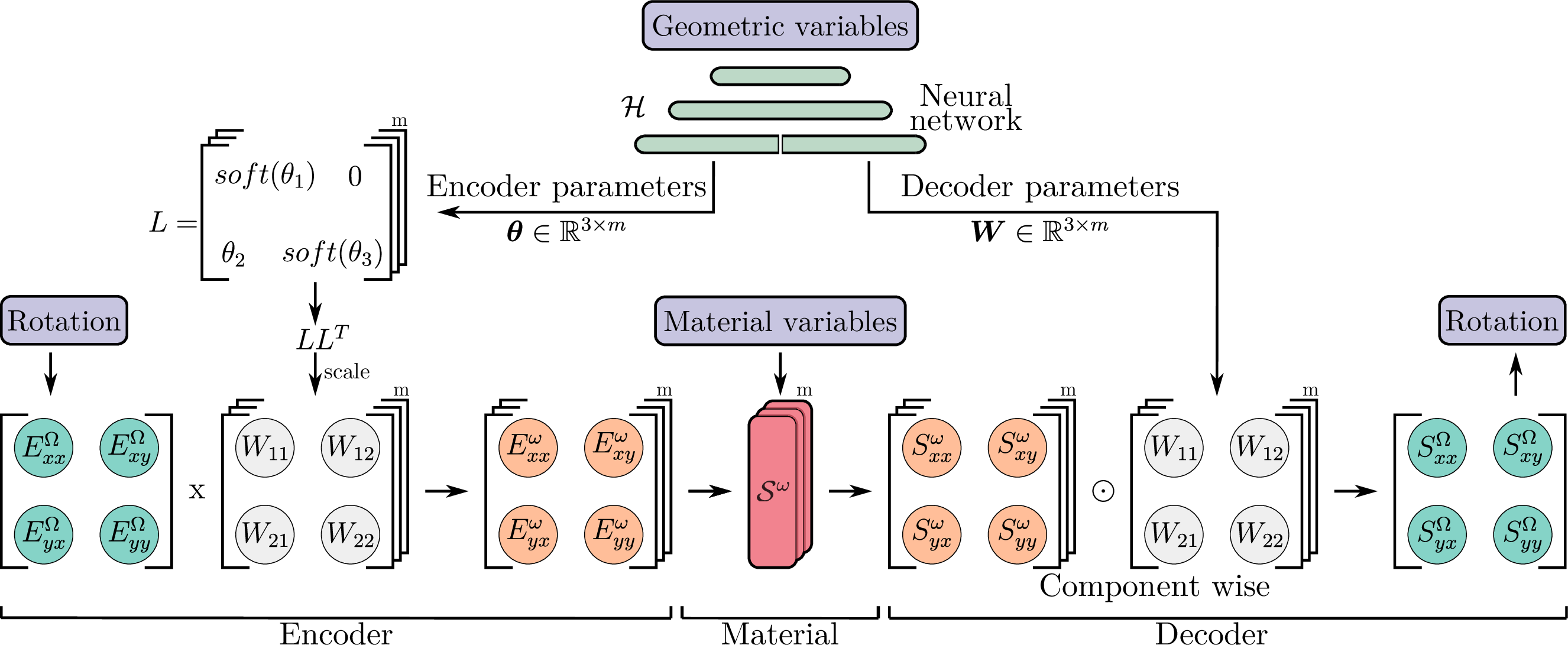
Geometric parameters of the microscale are used as inputs to \(\mathcal{H}\). Material parameters that affect the microscopic constitutive model can be directly modified in the fictitious material points on a per-sample basis. This has been shown to work even for large changes of parameters, and no retraining of the network is required [17]. Microscale orientations can be accounted for by rotating the input deformation and output stress accordingly.
5 Results: conditioning on microscale variables↩︎
In this results section, we compare a HyPRNN against a neural network and numerically validate it in a multiscale simulation, before performing a graded multiscale optimization.
5.1 Numerical setup↩︎
This section describes the software and modeling choices used for the numerical experiments. All code, as well as some pretrained surrogate models, is accessible on GitHub at https://github.com/SLIMM-Lab/hyprnn.
5.1.1 Parametrization and data generation↩︎
To train the surrogate models, a dataset is generated by simulating RVEs spanning a range of microstructural parameters. The RVEs consist of random packings of ellipses, representing the woodchips, surrounded by the mycelium. We consider four parameters: the ellipse aspect ratio \(r\), the woodchip volume fraction \(V_f\), the mycelium shear modulus \(\mu\), and the ellipse orientation \(\phi\). The first two are geometric parameters, and \(\mu\) is a material parameter As all ellipses follow the same orientation \(\phi\), it can be accounted for by rotating the deformation to align with the ellipse direction before passing it to the PRNN. Since we limit ourselves to 2D in this work, this is computed as: \[\bar{\mathbf{F}} = \mathbf{Q}^T \mathbf{F} \mathbf{Q}, \quad \mathbf{Q} =\begin{pmatrix} \cos\phi & -\sin\phi \\ \sin\phi & \cos\phi \end{pmatrix}.\] The output is then back-rotated to obtain the actual stress \(\mathbf{S}\). \[\mathbf{S} = \mathbf{Q} \bar{\mathbf{S}} \mathbf{Q}^T\] This way the orientation can be included by pre- and post-processing the surrogate’s inputs and outputs, and does not need to be included in the dataset.
The material variable \(\mu\) is included in the dataset, but it is not necessary for the random ellipse packing of the RVE. This packing is parametrized based on \(r\) and \(V_f\). \(V_f\) determines the number of ellipses, and \(r\) is are shared for all ellipses within one RVE. For a given aspect ratio, we compute the length and width of the ellipses such that the area of each ellipse remains constant, covering 0.8% of the RVE domain. Ellipses are then iteratively placed at random coordinates in a square domain until the desired volume fraction is reached. Ellipses crossing a boundary are wrapped to the opposite boundary to maintain a periodic geometry. If a newly placed ellipse overlaps with an existing one, it is discarded and a new random location is attempted. Gmsh [32] is used to mesh the domain. To produce a robust mesh, we verify that the number of nodes on opposite edges matches, and restart the procedure if this is not the case.
We simulate the RVEs using DOLFINx [33] with periodic boundary conditions. The load direction is selected randomly in \(\mathbf{F}\) space, and the RVE is loaded monotonically for 50 time steps up to \(\|\mathbf{F} - \mathbf{I}\| = 0.5\). If a time step fails to converge, the state is reverted to the last converged step, and the step is repeated with eight sub-increments. However, data from the intermediate sub-increments is not included in the dataset. If sub-increments also fail to converge, the simulation is stopped and only the steps up to the last converged step are included in the dataset.
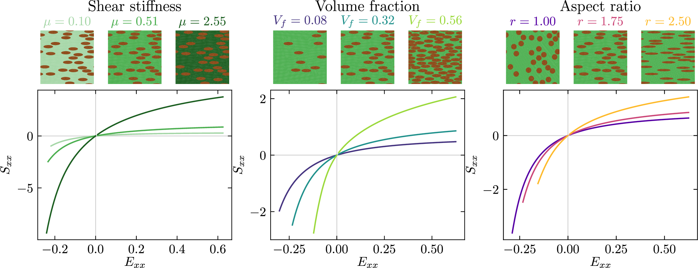
The influence of changing the microstructural parameters on the stress response is shown in Figure 6. In these responses, only the \(E_{xx}\) component is loaded for illustrative purposes. In tension, the simulations succeed for all 50 time steps. However, in compression, the simulations fail significantly earlier. Similar stress differences to those in this figure also occur for the other stress directions.
5.1.2 Surrogate model training↩︎
The HyPRNN, including the embedded material model, is implemented in JAX [34]. Two-thirds of the dataset is used for training, and the remainder is split evenly between validation and test sets. The training is done in \(\mathbf{E}\)-\(\mathbf{S}\) space, since their symmetry allows for reducing the input and output dimensions of the surrogates, which is generally advantageous for data-driven models. An L2 loss is minimized using the Adam optimizer [35], with a fixed learning rate of \(0.001\), until the validation loss has not improved for 50 epochs. All computations, including the training of the surrogates, are performed on a CPU. Just-in-time compilation and vectorized computations enable efficient training and inference. Since there is no history dependency considered here, all steps along a load path are computed in a single batched operation, together with steps from other load paths. A batch size of 2 load paths is used for all models.
5.1.3 Multiscale simulations↩︎
All macroscopic simulations are also performed in DOLFINx, where the dolfinx_materials [36] library enables the use of RVE micromodels and JAX-based surrogates as constitutive models. For surrogate-based multiscale simulations, automatic differentiation is used to compute the tangent stiffness tensor. Just-in-time compilation is used here too, resulting in a longer computation time for the first time step, but then enabling much faster subsequent steps. For the RVE-based multiscale simulations, we compute the tangents with central difference for ease of implementation. The RVE is solved with a solver tolerance of \(10^{-10}\), the central difference perturbation is \(10^{-8}\). The macroscale problem is solved with a tolerance of \(10^{-6}\). Substepping with eight sub-increments is applied at the macroscale in case of non-convergence. The micromodels are evaluated in parallel.
5.2 Conditioning comparisons↩︎
In this section, we compare the linear and nonlinear encoders of the HyPRNN. We additionally compare their performance to that of a standard neural network. Since PRNNs with a linear encoder can extrapolate material parameters after having been trained with only one [17], we first separately consider the effect of conditioning only on material parameters or only on geometric parameters, before combining them.
Three datasets, \(\mathcal{D}^{mat}\), \(\mathcal{D}^{geo}\), and \(\mathcal{D}^{all}\), are generated to test the influence of different microstructural parameters. For \(\mathcal{D}^{mat}\), only \(\mu\) varies, for \(\mathcal{D}^{geo}\), \(V_f\) and \(r\) change, and for \(\mathcal{D}^{all}\) all three parameters are varied. An overview is given in Table 1. The shear modulus \(\mu\) is selected randomly in the range \([0.10, 2.55]\). Since whole ellipses are placed one at a time, \(V_f\) is restricted to discrete increments. Rather than generating a new mesh for every \((V_f,r)\) combination that would arise from uniform sampling of \(r\), we draw from a predefined set of \((V_f,r)\) meshes. The combinations are a grid with \(V_f \in \{0.08, 0.16, 0.24, 0.32, 0.40, 0.48, 0.56\}\), and \(r \in \{1.00, 1.25, 1.50, 1.75, 2.00, 2.25, 2.50\}\), giving a total of 49 combinations.
| Parameters | # Samples | |||||
|---|---|---|---|---|---|---|
| 2-4 (lr)5-7 | \(\mu\) | \(V_f\) | \(r\) | Train | Val | Test |
| \(\mathcal{D}^{mat}\) | \([0.10,\; 2.55]\) | \(0.40\) | \(2.00\) | 2048 | 512 | 512 |
| \(\mathcal{D}^{geo}\) | \(0.51\) | \(\{0.08, \ldots, 0.56\}\) | \(\{1.00, \ldots, 2.50\}\) | 2048 | 512 | 512 |
| \(\mathcal{D}^{all}\) | \([0.10,\; 2.55]\) | \(\{0.08, \ldots, 0.56\}\) | \(\{1.00, \ldots, 2.50\}\) | 2048 | 512 | 512 |
We create learning curves for different hyperparameter settings of the neural network, the HyPRNN with a linear encoder, and the HyPRNN with a nonlinear encoder. For \(\mathcal{D}^{mat}\), no hypernetwork is necessary in the PRNN as \(\mu\) directly affects the fictitious material points. The ability of a PRNN to predict for different material parameters was already shown for plasticity in [17]. In contrast to that study, where only a single value is seen in training, the material parameter is varied in the training data here, in order to allow for a meaningful comparison with a neural network. The neural network, like the PRNN, predicts \(\mathbf{S}^{\Omega}\) from \(\mathbf{E}^{\Omega}\), with microscopic variables as additional inputs.
The hyperparameters include the choice of the activation functions and the network size, which for the PRNN corresponds to the number of material points. A more detailed overview of hyperparameters considered is given in 8. Each configuration is trained 10 times per number of training samples with different samples drawn from the training pool, and the average loss over these 10 training runs is plotted in Figure 7 (a). Each plot includes learning curves across a wide range of hyperparameters, and therefore different levels of complexity. This avoids having to either separately perform model selection for each dataset size, or first perform model selection on the largest dataset size and then risk biasing our results on smaller dataset sizes due to overfitting. The lowest average loss per type is marked with a circle, giving an envelope of the best models. The PRNN with a linear encoder performs well in the low-data regime and achieves a low loss with very few samples. Its loss plateaus after a certain number of training samples, when the NN and PRNN with a nonlinear encoder overtake it. The nonlinear PRNN starts from a higher loss than the linear PRNN, but does not suffer the same plateau.
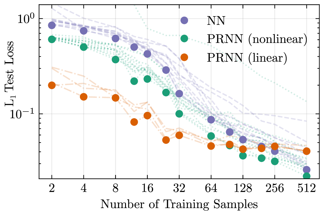

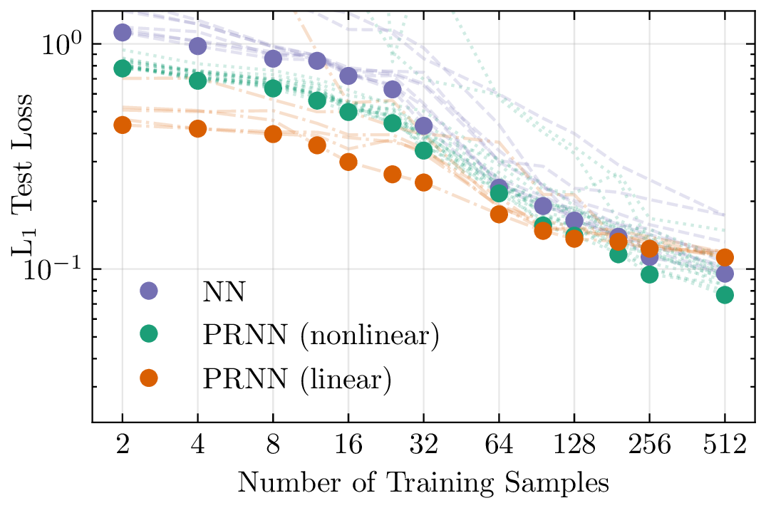
Figure 7: Overview of learning curves on the different datasets, plotted on a log-log scale. Each line represents the learning curve for one configuration of hyperparameters, averaged over 10 runs. The lowest point for each type of model (NN, linear (Hy)PRNN, nonlinear (Hy)PRNN) is highlighted to show the overall trend.. a — \(\mathcal{D}^{mat}\), b — \(\mathcal{D}^{geo}\), c — \(\mathcal{D}^{all}\)
The same process is repeated for \(\mathcal{D}^{geo}\), and the results are shown in Figure 7 (b). Here, the conditioning happens solely via the hypernetwork. A similar trend to before is observed, with the linear encoder performing better in the low-data regime, and the nonlinear encoder and neural network performing better for larger sample sizes. The error decreasing to a low value indicates that the hypernetwork approach to conditioning a PRNN is effective.
Figure 7 (c) shows the resulting learning curves for \(\mathcal{D}^{all}\), combining both the geometric and material parameters. The first thing that can be observed is that the error is higher than in the other two learning curve plots. This is because the dataset is more complex, and also reaches higher stress values, making the absolute difference larger than the relative difference in prediction. Due to the definition of the range of \(\mu\), the average \(\mu\) in \(\mathcal{D}^{all}\) is also higher than \(\mu\) in \(\mathcal{D}^{geo}\). The gap in Figure 7 (a) between the linear PRNN and the NN in the low-data regime is larger than the gap in Figure 7 (b), confirming the particular benefit that the linear PRNN offers in that it can transfer between different material property values without being trained for it. The nonlinear PRNN loss is closer to that of the NN, showing that it does not transfer material properties as well as a linear PRNN. This is because the nonlinear PRNN relies less strongly on the physics in the material model for reproducing the data.
For all the datasets, the differences between the types of models are significant, and variations for specific hyperparameters within one type are smaller. This indicates that the overall results are not overly sensitive to the specific settings used, such as the number of material points or a specific number of neurons in a layer. Sigmoid activation performs much better than ReLU activation in all networks (NN, nonlinear encoder, hypernetwork). Furthermore, HyPRNN models with only the mycelium material points perform better than those with additional woodchip material points when there is little available data. These effects on the learning curves are shown in 8. We suspect that the large contrast between the stiffness of the mycelium and the woodchip degrades training performance. This phenomenon deserves more attention in future work.
A test curve from \(\mathcal{D}^{all}\) with predictions from several representative models is visualized in Figure 8 with pair-wise stress-strain plots. For this specific curve, all surrogates predict the same overall shape, but quantitatively the nonlinear HyPRNN performs best. The NN trained with 32 samples shows a significantly higher error compared to the other curves. The nonlinear HyPRNN used here has twelve material points, a single hidden layer in the encoder, and three hidden layers in the hypernetwork, which is eight nodes wide and uses sigmoid activations. The linear HyPRNN has six material points and a hypernetwork with a single hidden layer with sigmoid activation. The neural network has four hidden layers of 64 nodes, with sigmoid activation.
![Figure 8: For specific model architectures, the instances with the median test losses are selected (out of 10 training runs) such that the responses represent that of a single training run. For these models, predictions are made on the sample for which the nonlinear HyPRNN has the median error. The legend description is as follows: [model name (number of training samples), error on this sample, rank of sample error out of all test errors (1 is best, 512 is worst)]. All other models perform worse on this sample than on their median sample, making the quality of their predictions in this plot lie on the conservative side.](/article/2607.13688/figures/median_curves_test.png "fig:")
5.3 FE\(^\mathrm{2}\) validation↩︎
Dataset losses quantify pointwise accuracy, but do not fully correlate with the surrogate performance in a full FE\(^\mathrm{2}\) simulation. The nonlinear interactions between the points might cause the solution to drift, the tangent stiffness plays a direct role, and the distribution of explored points differs from the test set distribution. We therefore validate our method on a simple structural example: a 3-point bending beam. The beam measures \(4.0 \times 0.3\) [m], and is displaced vertically at midspan by \(0.05\) [m] in five increments of \(0.01\) [m]. Symmetry is used to simulate only the left half of the beam, fixing the bottom left corner, and preventing horizontal movement at the symmetric edge. Note that this setup somewhat overconstrains a typical 3-point bending beam, as it does not allow for any horizontal movement. The applied grading of the simulation is shown in Figure 9, spanning a wide range of the considered parameters. The volume fraction gradually increases along the beam height; the shear modulus increases towards the beam center. The woodchip aspect ratio and orientation, in contrast, jump discontinuously between an inner and an outer band along the height.

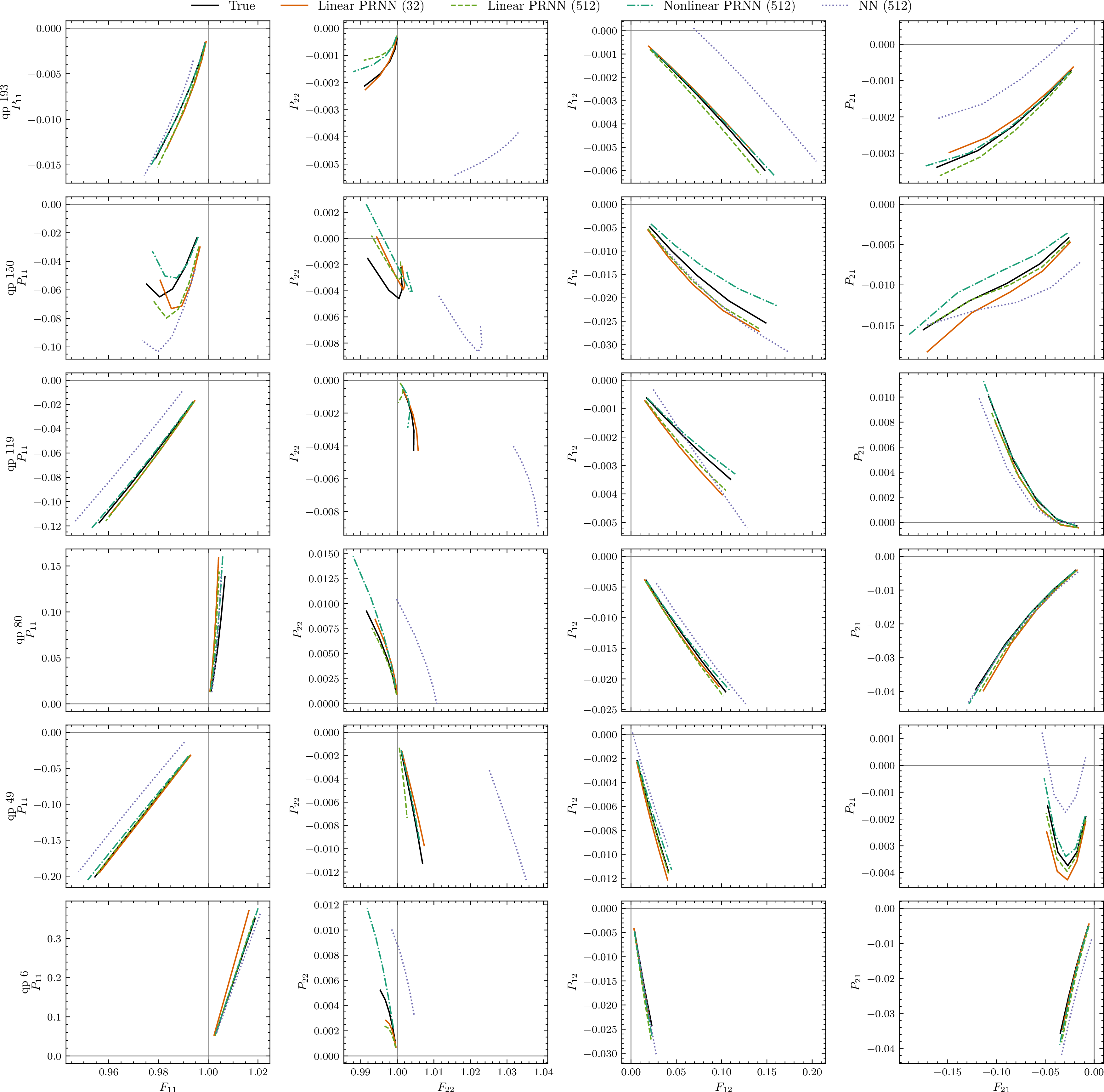
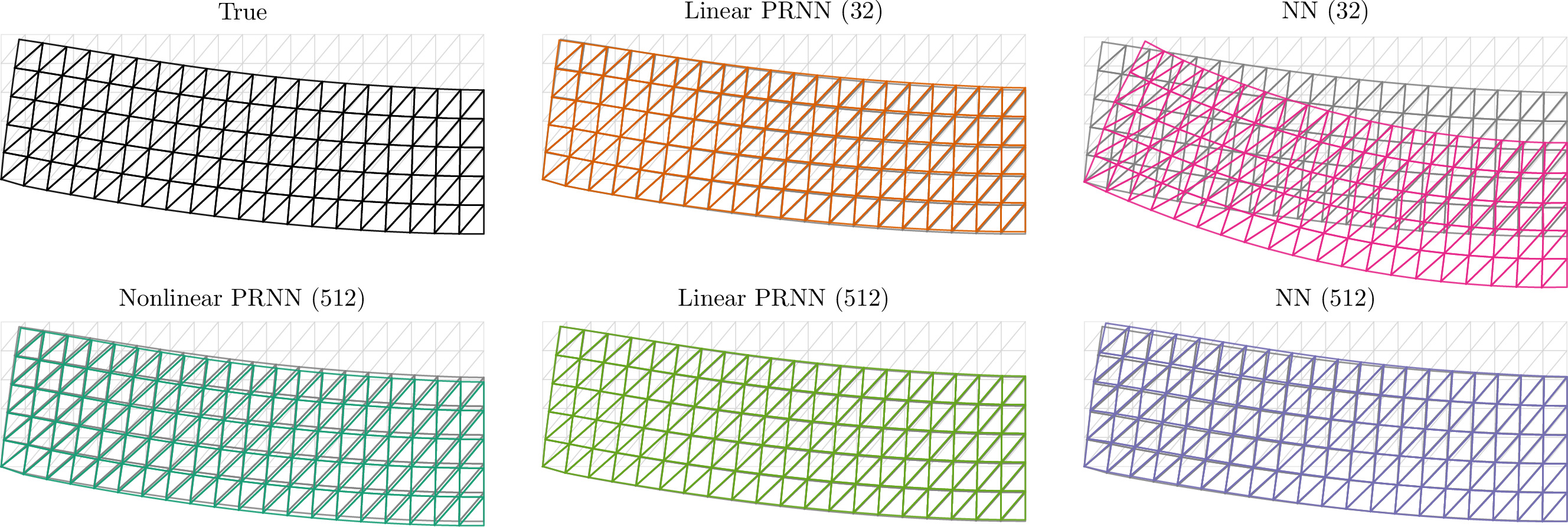
For the linear HyPRNN and the NN, two variations are considered, one with 32 training samples and one with 512 training samples. For the nonlinear HyPRNN, we only consider a model trained on 512 samples. A comparison of the displacement fields of surrogate-based simulations to the RVE-based simulation is visualized in Figure 10. All HyPRNN-based surrogates show relatively good agreement, and the linear HyPRNN with 512 samples shows a near-perfect match. While the NN and nonlinear HyPRNN with 512 samples have lower errors on the test set, their displacements in these multiscale simulations are less accurate than the linear HyPRNN. The NN with 32 samples shows very poor performance. In 9, the stress strain paths at a few quadrature points are shown, clearly showing how the neural network surrogate produces a nonzero stress in the undeformed state, whereas the HyPRNN models do not.
We compare the computational cost of the different simulations. All computation times are obtained on a standard desktop PC with an Intel Xeon W-2223 processor. As discussed earlier, the RVE-based simulation uses central differences to compute the tangent, which is suboptimal in terms of the simulation time. The results are presented in Table ¿tbl:tab:fe295time?, showing the much lower simulation time with the surrogate models. The data generation and training times are one-time costs, whereas the online simulation time is repeated for each new graded simulation. Still, this large data generation time illustrates the relevance of data requirements for surrogate modeling in multiscale analysis. The first and remaining time steps are reported separately, since the first time step includes the just-in-time compilation of the surrogates. The stark contrast between the RVE and surrogate based simulation time highlights the benefit of surrogate-based simulations. This contrast would only increase for larger macroscopic simulations with more elements, or those running for more time steps.
ll ccccc & RVE & Linear & Linear & Nonlinear & NN
& & PRNN (32) & PRNN (512) & PRNN (512) & (512)
& Data generation & – & 2035.97 & 32575.51 & 32575.51 & 32575.51
& Training & – & 93.88 & 336.61 & 1134.89 & 410.09
& Total & 5900.52 & 1.27 & 1.75 & 2.12 & 1.00
& Initialization & 137.49 & 0.15 & 0.17 & 0.44 & 0.37
& Time step 1 & 965.75 & 1.03 & 1.52 & 1.56 & 0.59
& Time steps 2-5 & 4797.27 & 0.08 & 0.05 & 0.12 & 0.04
5.4 Graded multiscale optimization↩︎
We now turn to using our surrogate as a constitutive model to optimize a multiscale graded material. Disks subject to rotation or internal loads are commonly studied in the functionally graded materials literature [37]–[39], where a graded thickness is typically used to reduce peak stresses. We adopt a similar setup but grade the microstructural parameters rather than the thickness under an internal pressure. An overview of the structure and boundary conditions is provided in Figure 11. The goal is to minimize peak stresses. The parameters only vary radially, allowing for a 1D parametrization. The aspect ratio and woodchip angle are combined into \(r_{\mathrm{combi}}\) to enable rotated woodchips in a radially consistent manner. Specifically, \(r_{\mathrm{combi}} \in [0.4, 2.5]\), where values below one are equivalent to setting \(r=1/r_{\mathrm{combi}}\) with angle \(\phi=\ang{90}\) with respect to the radial direction, while for values above one, \(r=r_{\mathrm{combi}}\) and \(\phi=\ang{0}\). In this parametrization, the woodchips can thus only be either parallel or perpendicular to the radial direction. The optimization variables are thus \(V_f\), \(r_{\mathrm{combi}}\), and \(\mu\).
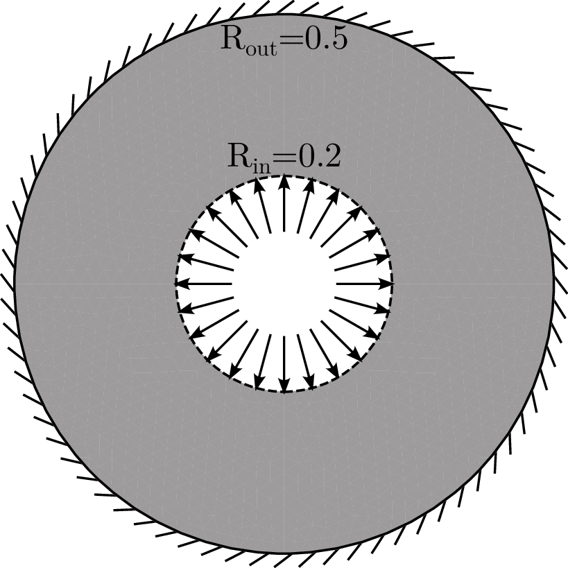
The optimization problem is defined as minimizing the peak Cauchy stress under a given load, subject to a maximum acceptable deformation. Accounting for symmetry, only one quarter of the disk is simulated. The maximum acceptable deformation is set to 0.05 (16.6% of the thickness) through a linearly scaling penalty on the loss when exceeded. We use the Covariance Matrix Adaptation Evolution Strategy (CMA-ES) [40], an off-the-shelf, iterative, derivative-free algorithm, to optimize our objective function. Alternative optimization algorithms, such as Bayesian optimization, are also expected to work, and the choice of optimizer is not expected to affect our conclusions.
![Figure 12: The optimized graded structures and their resulting average stresses. The average stresses are obtained by first computing the Cauchy stress, and then using the von Mises formula. The maximum stresses are 4.51, 2.73, and 2.59 [MPa] for the random, uniform, and graded structure respectively. The von Mises plot shows the stresses in the deformed configuration.](/article/2607.13688/figures/disk_grading_comparison.png "fig:")
Three cases are compared: one random, one uniform, and one graded with four control points per variable through the thickness, between which the values are linearly interpolated. The first of these is included as an unoptimized reference solution, while the other two represent optimization problems with increasing flexibility (three versus twelve parameters). For the random initialization, the angle and aspect ratio are randomly chosen, \(\mu\) is set to 1.5, and the volume fraction is modified to exactly satisfy the deformation constraint using the bisection method, leading to a peak stress of 4.51 [MPa]. The optimized results are visualized in Figure 12. An efficient uniform parametrization with a low peak stress of 2.73 [MPa] is reached after 240 simulations. The graded structure further decreases this peak stress to 2.59 [MPa] after 1006 simulations. The optimization finds that decreasing the volume fraction and setting \(r_{\mathrm{combi}}\) below one is better inside the disk, rather than directly at the edge.
6 Results: conditioning on manufacturing variables↩︎
Precisely controlling the microscale geometry as assumed in Section 5 is not yet feasible for most materials. Manufacturing process variables influence the microscale, but finding an exact relation between these variables and the microscale geometry is not straightforward. We therefore showcase the ability to condition the PRNN on variables from the manufacturing process. This serves as a computational proof-of-concept aiming to inspire future experimental work.
Mycelium-woodchip composites can be created by depositing woodchips from a bag or container into formwork, and then inoculating them with mycelium. We simulate this deposition process and consider two variables in the process. First, small round mycelium pellets can be added to the mix, decreasing the resulting woodchip volume fraction. We assume that these have the same material properties as the mycelium that grows in the formwork. Second, the initial orientation of the dropped woodchips can be controlled, for example by using a sieve, resulting in anisotropy.
6.1 Dataset↩︎
To mimic the deposition process of the woodchips, we use Yade, a discrete-element method simulator [41]. The general approach involves initializing the woodchips as clumps of spheres, and dropping them inside a 3D box with gravity. As we focus here on demonstrating our approach, we make the pragmatic choice of not calibrating against experiments. Each woodchip is modeled as a rigid stack of connected spheres. All woodchips are initialized with the same orientation \(\theta\), as visualized in Figures 13 (a) & 13 (b), but a small random velocity is added to each to avoid an unrealistically aligned result. As a result, most woodchips deviate to some extent from their initial orientation, but the remaining effect does lead to anisotropy. The pellets are modeled as single spheres, with a radius 1.5 times as large as the spheres in the woodchips. We control the pellet fraction: the ratio between the volume of the pellets and the volume of the woodchips before deposition. An example of a settled deposition is visualized in Figure 13 (c).
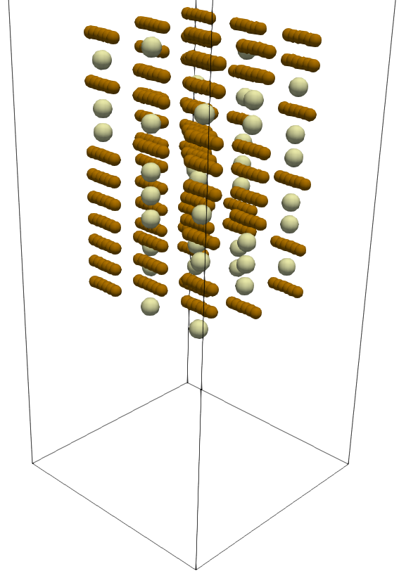
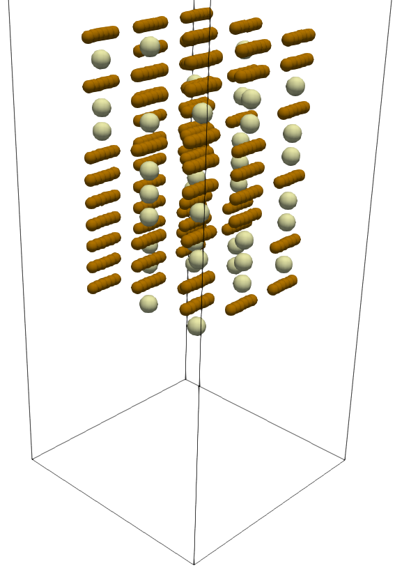
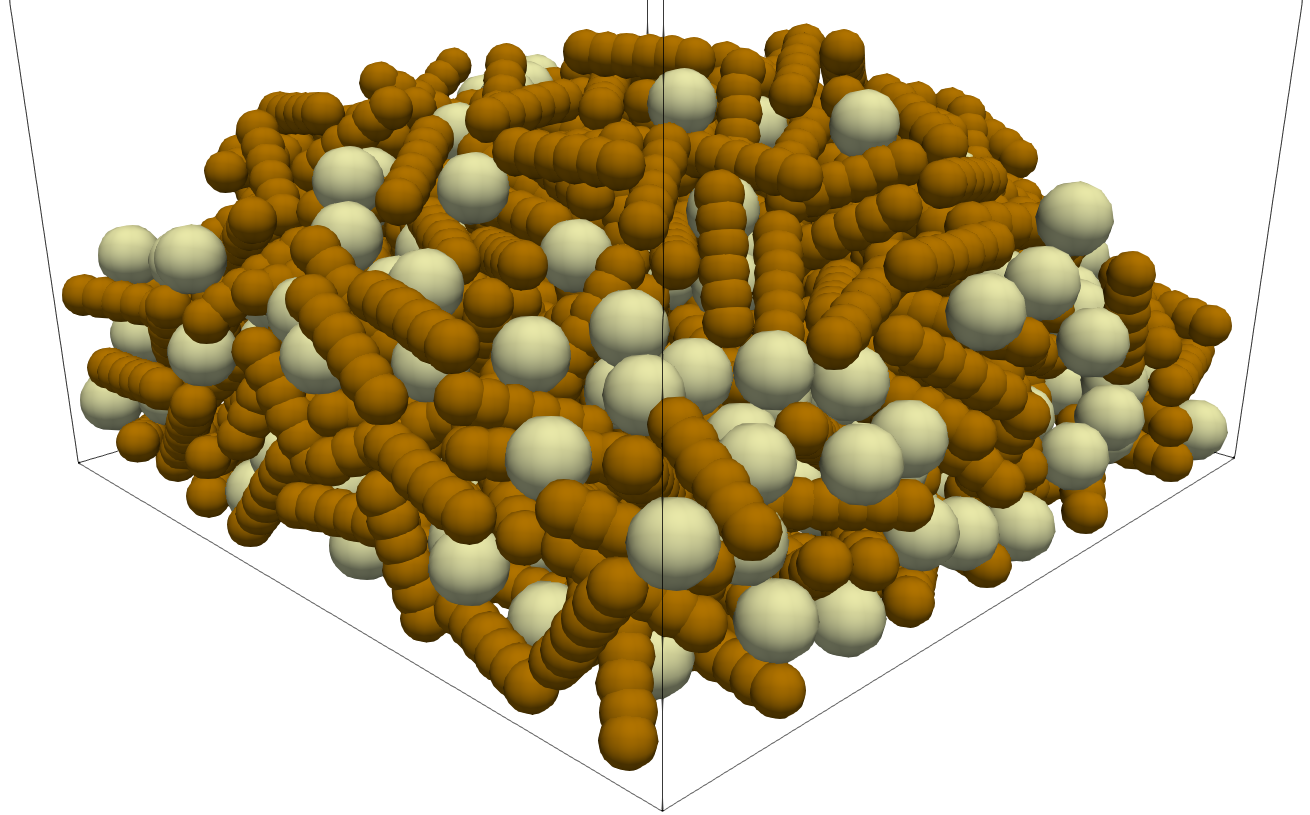
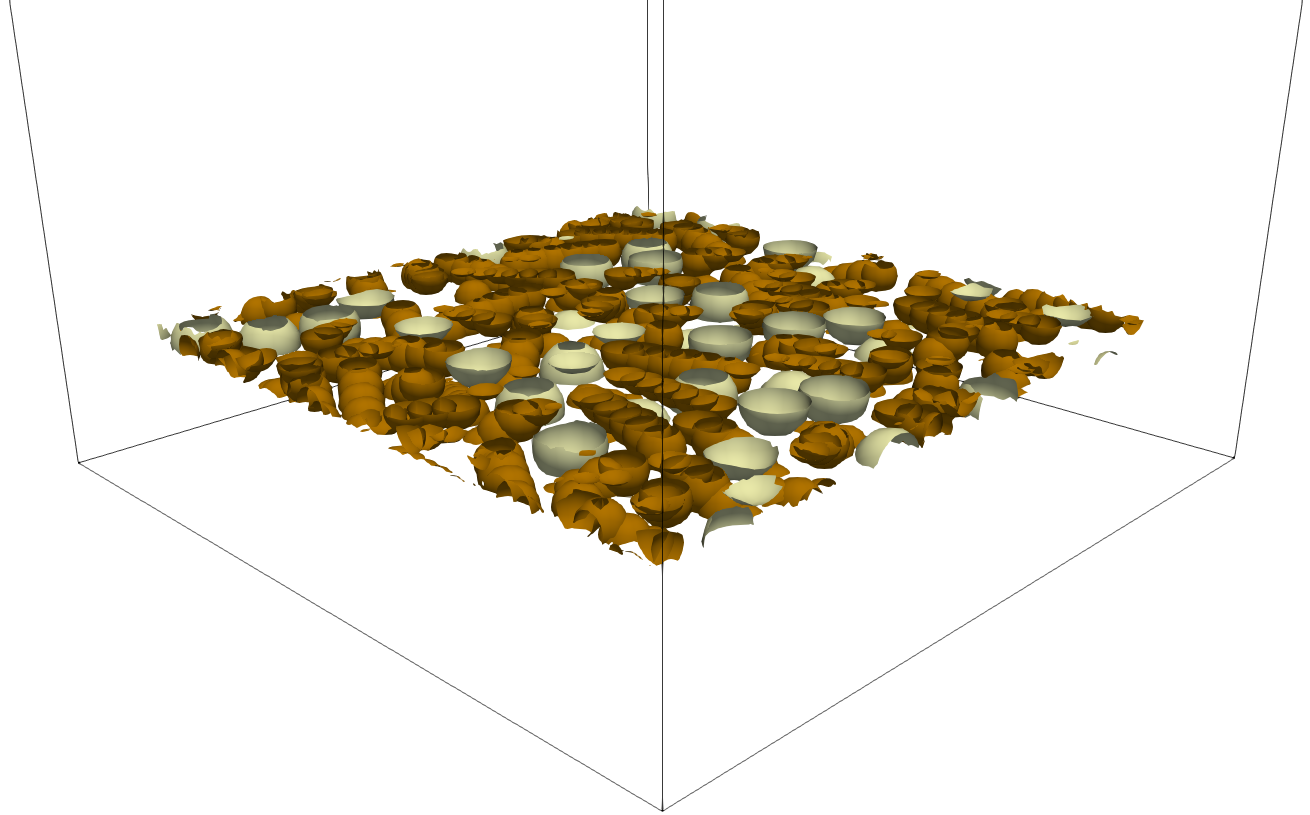
Figure 13: 3D visualizations of the deposition process with a 30% pellet fraction. The settings differ between the visualizations. In the actual deposition, the woodchips and pellets are smaller and more numerous than shown here.. a — Initialization \(\theta=\)0°, b — Initialization \(\theta=\)90°, c — Settled deposition, d — Sliced section
Once the woodchips have settled, the configuration is sliced by a horizontal plane at a height of four times the radius of the spheres used to model the woodchips, as shown in Figure 13 (d). Only a central section of the box is included to avoid boundary effects of the 3D deposition. Each intersected sphere is mapped to a disk in a 2D simulation (without gravity), whose radius equals the radius of the sphere’s cross-section at the cutting height. This 2D simulation has periodic boundary conditions, and a relaxation phase allows clumps that were overlapping other clumps at the boundary to untangle. Then, a convex hull around each clump is drawn, before shrinking each hull to avoid overlap. Finally, this geometry is meshed using Gmsh to create a periodic 2D mesh, as shown in Figure 14. Only meshes from a single initial orientation are required since it can be accounted for by rotating the deformation and stress tensor as discussed in Section 5.1.1; here we set the initial orientation to 0°.
This approach of taking a 2D slice from the 3D deposition does somewhat disconnect the manufacturing variable from the generated microstructure; the final model used is only indirectly related to the process that simulated it. Ideally, the 3D deposition would be directly used, but we transfer it to 2D to reduce the computational cost of simulating the mechanical behavior of the microstructures. The resulting meshes are subjected to monotonic loading in random directions to create a dataset. Since the HyPRNN is conditioned on fewer parameters than before, we create a smaller dataset consisting of 512 samples, 256 used for training, and 128 each for validation and testing. The dataset is visualized in Figure 15. A HyPRNN with linear encoder is trained on this dataset.
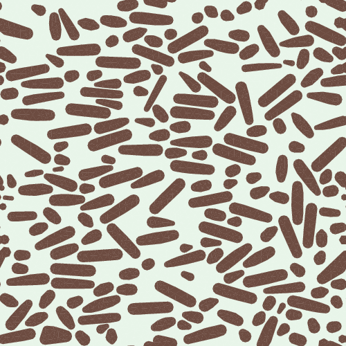

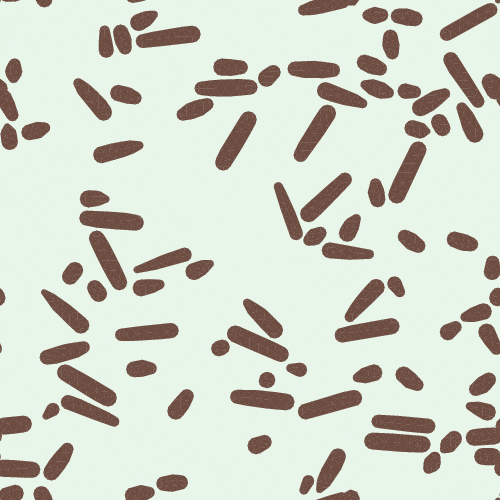
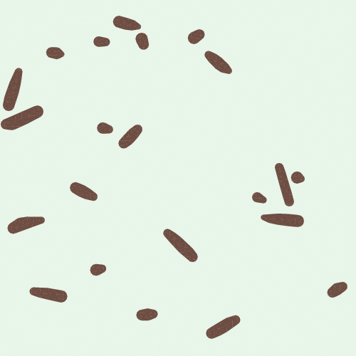
Figure 14: Generated 2D microstructures for various pellet fractions, all with an initial orientation of 0°.. a — Pellet fraction: 0%, b — Pellet fraction: 30%, c — Pellet fraction: 60%, d — Pellet fraction: 90%
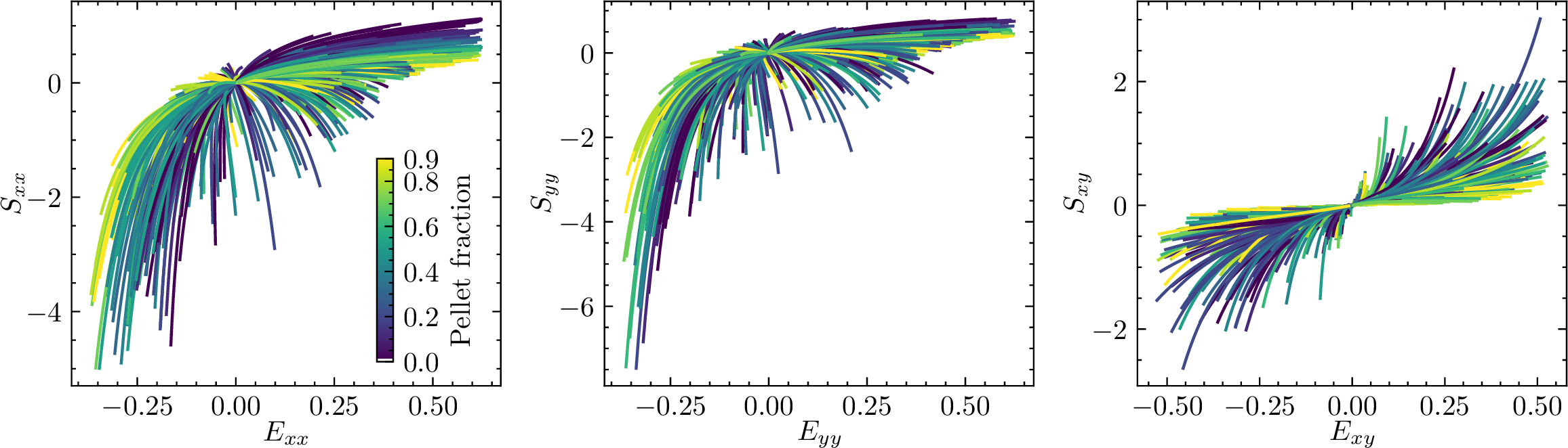
6.2 Deformation optimization↩︎
Next, we study whether the manufacturing variables can lead to a noticeable difference in a sample’s deformation. A compression test is simulated for a square sample with a hole; the setup is visualized in Figure 16 (a). The objective is to minimize the horizontal deformation of the hole, which we denote as bulging and quantify as: \(u^R_x - u^L_x\), where \(R\) and \(L\) refer to the respective nodes in Figure 16 (a). The top plate is gradually lowered for a total deformation of 20% of the sample height. This loading is imposed with a contact model using the penalty method in order to replicate a compression test and allow for separation from the plate. Since creating a continuous grading is challenging in practice, we instead partition the domain into hexagonal regions. Using symmetry, this results in 13 regions for a total of 26 parameters to optimize. The optimizer settings are identical to those of Section 5.4.
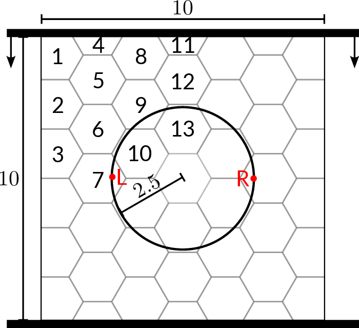

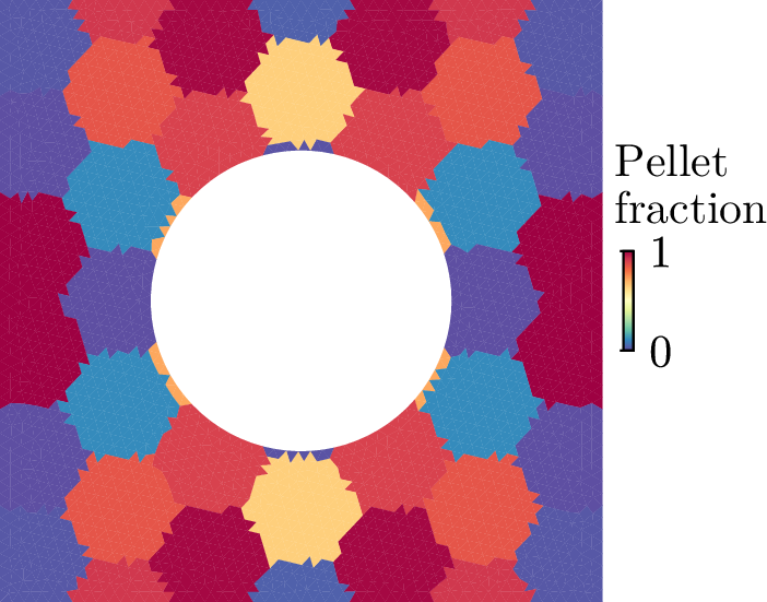
Figure 16: Simulation setup and results of the deformation optimization.. a — The thirteen parametrized regions are numbered., b — Optimized \(\theta\), c — Optimized pellet fraction
We compare the optimized result to a baseline case with 0% pellet fraction and a random orientation in each element. The colormap used in Figure 16 (a) shows the optimized pellet fraction. The resulting microstructure distribution and deformations are visualized together in Figure 17. A clear difference is observed, with the baseline bulging significantly outward, whereas the optimized result barely moves horizontally. The optimized pattern shows an X-like structure that forms bands from the corners of the sample to the L and R points. Next to the bands there are parts with intermediate pellet fraction. The optimized pattern of the orientation is far from trivial. To verify the effectiveness of the orientation, we rerun the simulation with the optimized pellet fraction but a fixed orientation of \(\theta\)=90°, which leads to a worse result with a bulge of 0.0623. This example demonstrates how a HyPRNN can be used to find the manufacturing variables that lead to a desired mechanical behavior.
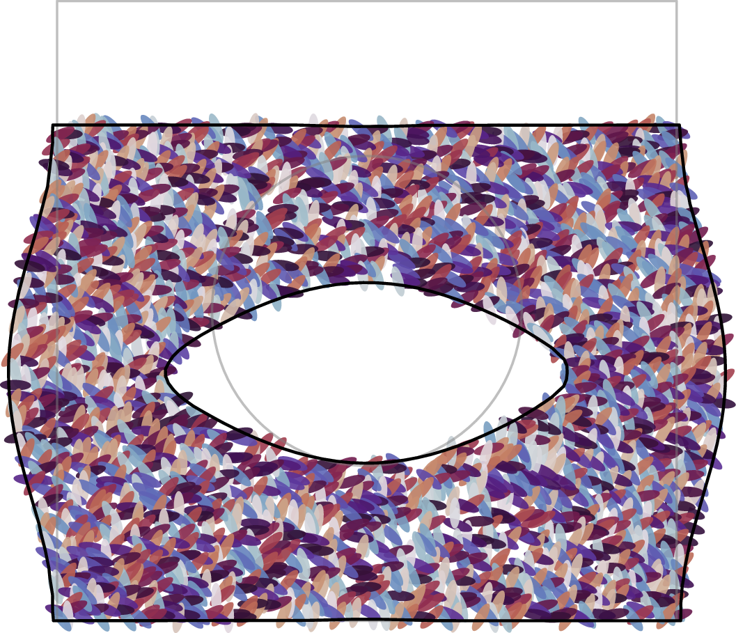

Figure 17: Deformed results from the baseline and optimized compression test. The ellipses represent both manufacturing variables: their sparsity depends (inversely) on the pellet fraction, and their orientation directly reflects their initial deposition orientation. Note that the size of the ellipses does not reflect the scale of the woodchips, for which we assume a separation of scales.. a — Baseline: bulge = 1.48251., b — Optimized: bulge = 0.00001.
7 Conclusion↩︎
In order to develop a surrogate model for a range of different microstructures, we propose a HyPRNN: a PRNN conditioned on microstructural variables using a hypernetwork. The finite-strain HyPRNN encoder was modified to guarantee valid responses, even for large deformations. The physics-based inductive bias allows the HyPRNN with linear encoder to perform very well in the low-data regime. An additional nonlinear encoder was introduced that performs better than the linear encoder when more data is available. An advantage of using a HyPRNN is that material parameters, such as the shear modulus, can be varied directly in the embedded constitutive models. Geometric properties, such as the volume fraction, are passed as inputs to the hypernetwork. We handled orientations of the microstructure by training with one fixed orientation, and then pre- and post-processing the surrogate’s inputs and outputs to account for the orientation. This conditioned surrogate model enabled graded multiscale simulations. For a simple 3-point bending experiment of a graded multiscale beam, the surrogate-based simulations reduced the computation time from 5900 seconds to 2 seconds, while maintaining high accuracy. By performing a multiscale optimization, we showed the ability to find a material grading that significantly reduces peak stresses.
We circumvent the need for an additional model to parametrize microstructural geometries (e.g., a conditional variational autoencoder or a conditional denoising diffusion model) and instead condition directly on the manufacturing variables used to generate the microstructure. Specifically, we conditioned the HyPRNN on inputs from a discrete-element simulation that mimics the deposition of woodchips and mycelium pellets. The resulting model was used in an optimization loop to substantially alter the deformation pattern of a sample under compression. Overall, this work highlights the necessity of microstructure-aware data-driven surrogates for multiscale simulations. Furthermore, we demonstrate the potential that precise control of microstructural variables can bring.
Acknowledgements↩︎
JS, IR, and FM gratefully acknowledge the TU Delft AI Labs programme for enabling this work. SS and KM are supported by the ERC Consolidator Grant, AM-IMATE, 101088968. We also acknowledge Martin Lesueur and Winston Lindqwister for the insightful discussions.
8 Hyperparameter configurations↩︎
In Table 2 we present the hyperparameters used to create the learning curves and compare the model performance. A wider range was explored in earlier prototyping. We did not perform a full grid sweep over the possible settings for each model, but followed a more manual iterative process. For example, for the neural network, we found that reLU performed worse than the other activations, and therefore did not try all model sizes with it. For the hypernetwork, we further considered an alternative setup that scaled the hidden layer sizes depending on the number of its outputs (the number of encoder weights), but found no gain.
| Hyperparameter | HyPRNN Nonlinear | HyPRNN Linear | NN |
|---|---|---|---|
| Material points | 2, 3, 6, 12, 24, [6,3] | 2, 3, 6, 12, [6,3] | – |
| Hypernetwork hidden sizes | (8), (8,8,8) | (8), (8,8,8) | – |
| Hypernetwork activation | sigmoid, reLU | sigmoid | – |
| Encoder activations | softplus, sigmoid, reLU | – | – |
| Encoder hidden sizes | (8), (8,8,8), (16), | – | – |
| (16,16,16) | |||
| NN Activations | – | – | sigmoid, tanh, reLU |
| NN hidden sizes | (8,8), (16,16), (16,16,16), | ||
| – | – | (32,32,32), (64,64), (64,64,64), | |
| (64,64,64,64), (128,128,128) |
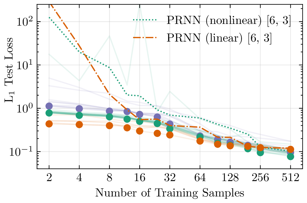
In Figure 18 we highlight learning curves for models with woodchip material points, one for the nonlinear and one for the linear PRNN. The woodchip material points cause significantly worse losses in the low-data regime. Given sufficient data, the models learn to make good predictions, but are still among the worst relative to other configurations.
9 FE\(^\mathrm{2}\) validation stress paths↩︎
In Figure 19 we plot the stress strain paths of several quadrature points from during the simulations in Section 5.3. We omit the results of the NN (32) surrogate, as its errors are high, and including its paths requires a substantial increase of the axes bounds, making the other paths more challenging to compare. This figure clearly demonstrates how the NN is not constrained to have zero stresses in the undeformed state, showing a significant bias. All PRNN models closely follow the ground truth response.