Optimal and Efficient Contextual Combinatorial Semi-bandits with General Function Approximation
July 15, 2026
Abstract
We study the contextual combinatorial semi-bandit (CCSB) problem with general reward function approximation. At each round, the learner observes a context, selects a combinatorial action consisting of a subset of basic arms, and receives the reward of each selected arm; the goal is to maximize the cumulative reward over time. We propose SquareCB.Comb, a computationally efficient algorithm that, at each round, solves a convex optimization problem to sample a combinatorial action that balances exploration and exploitation. SquareCB.Combscales to large arm sets and imposes no structural assumptions on the action set beyond a cardinality bound of \(m\) on each combinatorial action. We prove that SquareCB.Combachieves a minimax optimal regret bound of \(\iupbound{\sqrt{m A T \log \abs{\Fcal}}}\), where \(A\) is the number of arms, \(m\) is the maximum number of arms in a combinatorial action, \(T\) is the time horizon, and \(\Fcal\) is the reward function class. In the realizable setting, this bound matches the state-of-the-art regret guarantees achieved by policy search-based algorithms in the more restricted slate recommendation settings, while simultaneously generalizing to arbitrary combinatorial action structures and general reward function approximation.
1 Introduction↩︎
The contextual combinatorial semi-bandit (CCSB) problem is a framework for sequential decision making in which the learner repeatedly selects a subset of base arms (a combinatorial action) based on observed contextual information, with the goal of maximizing cumulative reward over time. For example, [1] formulate bottleneck identification in road networks as a CCSB problem, where the learner repeatedly selects a source-to-destination path (a subset of road segments) and seeks to minimize the largest travel cost along the chosen path, using contextual side information such as time of day and traffic conditions. As another example, [2] formulates online routing for multi-LLM serving as a CCSB problem with knapsack constraints, where for each incoming user query the learner selects a subset of LLMs (a combinatorial action) to invoke subject to a token-budget cap and seeks to maximize the resulting response quality. Other applications include energy-efficient path planning for vehicle navigation [3], online personalized slate recommendation [4], [5], and resource allocation in wireless networks, including channel assignment [6] and beam management [7].
A CCSB environment is specified by a context space \(\Xcal\) and an arm set \(\Acal\) of size \(A\). The combinatorial action space \(\Scal \subseteq \cbr{0,1}^A\) is a feasible family of subsets of \(\Acal\) determined by the problem structure (e.g., the \(m\)-set setting [8] or knapsack constraints [2]). At each round \(t\) of interaction, the environment shows a context \(x_t\) to the learner, together with a vector \(r_t \in [0, 1]^\Acal\) representing the reward of each arm, hidden from the learner. The learner selects a combinatorial action \(s_t \in \Scal\) based on \(x_t\), observes the semi-bandit feedback \(\cbr{r_t(a) : s_t(a) = 1}\), and receives reward \(\inner{r_t}{s_t} = \sum_{a: s_t(a)=1} r_t(a)\). The goal is to minimize the regret over \(T\) rounds, defined as the gap between the cumulative reward of the optimal context-dependent action in hindsight and the algorithm’s expected cumulative reward.
Prior works on contextual combinatorial semi-bandits with function approximation focus on the linear-reward setting, in which the expected reward of each arm is a linear function of the context [9]–[11]. In many real-world applications, however, the mapping from context and arm to reward is not strictly linear. For instance, user clicks in online recommendation systems often exhibit highly non-linear dependence on contextual features. In this work, we consider a general function approximation setting for CCSB, where the mapping from the context to the expected reward of the arms is assumed to lie in some known function class \(\Fcal\).
1.0.0.1 Our contributions.
We propose an algorithm, SquareCB.Comb, for the CCSB problem with general reward function approximation. Our algorithm builds on the Estimation-to-Decisions principle for online decision making [12], which lets the algorithm balance exploration and exploitation and yields a regret bound of \(\iupboundlog{\sqrt{m A T\log\abs{\Fcal}}}\), where \(m\) is the maximum number of arms in a combinatorial action, \(A\) is the number of arms, \(T\) is the time horizon, and \(\Fcal\) is the reward function class.
This bound matches the best known regret rate for the linear-reward setting and extends it to general reward function approximation.
| Algorithm | ||||
| Setting | ||||
| Constraint | ||||
| Type | ||||
| Guarantee | ||||
| [8] | ||||
| adversarial reward | ||||
| \(m\)-ordered slate | Policy | \(\iupboundlog{\sqrt{m A T \log(\abs{\Pi})}}\) | ||
| SquareCB.lin [13] | ||||
| stochastic reward | General | Value | \(\iupboundlog{m\sqrt{AT \log(\abs{\Fcal})}}\) | |
| SquareCB.comb (ours) | ||||
| stochastic reward | General | Value | \(\iupboundlog{\sqrt{m A T \log(\abs{\Fcal})}}\) |
2 Related Work↩︎
2.0.0.1 Contextual combinatorial semi-bandit (CCSB) with linear function approximation.
Motivated by personalized recommendation, [9] first introduced the contextual combinatorial semi-bandit (CCSB) problem under the assumption that the expected reward of each arm is linear in the context with a shared \(d\)-dimensional coefficient, while the reward of a combinatorial action may be a general function of the per-arm rewards. They proposed C\(^2\)UCB, a UCB-based algorithm with an \(\iupbound{\sqrt{(d+m) d m T}}\) regret guarantee. [14] studied a variant of the CCSB problem with a cascade feedback structure and proposed an algorithm with \(\iupbound{\sqrt{d m T}}\) regret under a (strong) feedback coverage assumption. [11] gave a refined analysis of C\(^2\)UCB and obtained a minimax optimal regret guarantee of \(\iupbound{d\sqrt{m T}}\). In comparison, our algorithm, instantiated with a discretization of the linear reward function class, attains regret \(\iupboundlog{\sqrt{m A d T}}\) in this setting.1 [15] studied the adversarial linear rewards CCSB problem, where each arm’s linear reward coefficient is chosen adversarially, and proposed a follow-the-regularized-leader (FTRL) algorithm with \(\iupbound{\sqrt{T}}\) regret. [16] generalizes the results of [11], [14] to linear contextual combinatorial bandits with probabilistically triggered arms; when instantiated in the setting of [14], their result replaces the minimum triggering probability assumption with a natural assumption on the reward function. [10] gave the first best-of-both-worlds algorithm for linear CCSB, attaining \(\iupbound{\sqrt{T}}\) regret in the adversarial setting and \(\iupbound{\log T}\) regret in the stochastic setting by combining FTRL with a negative Shannon entropy regularizer.
2.0.0.2 Contextual combinatorial semi-bandit (CCSB) with general function approximation.
[17] studied the contextual MDP (CMDP) problem with adversarial losses, which can be used to solve the contextual shortest-path problem as a special case. On a graph with \(N\) nodes and \(M\) edges, the shortest-path instance can be cast as an episodic CMDP with episode length \(N\); under this reduction, their algorithm attains regret \(\iupboundlog{\sqrt{N^{7} T \log\abs{\Fcal}}}\), which is worse than our bound \(\iupboundlog{\sqrt{N M T \log\abs{\Fcal}}}\) in this setting (see 4.1 for details). [18] studied the general function approximation with a Lipschitz continuity assumption and proposed algorithms based on the Thompson sampling and UCB principles, achieving \(\iupboundlog{\sqrt{m \tilde{d} T}}\), where \(\tilde{d}\) is the effective dimension of the neural tangent kernel associated with the reward function class.
Another line of work approaches CCSB via policy search: the learner is given a policy class \(\Pi\) and seeks to minimize regret against the best policy in \(\Pi\) in hindsight. The early work of [8] proposed algorithms based on exponential weighting over the policy class, achieving \(\iupboundlog{\sqrt{m A T \log(\abs{\Pi})}}\) regret in the unordered and ordered slate settings with \(n\) items (where \(A = n\) and \(mn\) respectively). Their algorithm is computationally inefficient as it requires enumerating all policies in the policy class. Subsequently, [19] studied CCSB with a linearly weighted reward structure and proposed the VCEE algorithm, which improves computational efficiency by extending the policy elimination technique of [20] to call a cost-sensitive classification oracle over the policy class rather than enumerating all policies. Their regret guarantee ranges between \(\iupboundlog{\sqrt{mAT\log\abs{\Pi}}}\) and \(\iupboundlog{m\sqrt{AT\log\abs{\Pi}}}\), depending on the reward structure. [21] studied CCSB in both the PAC guarantee and the regret minimization settings, and adapted the technique of [20] to construct an importance-weighted sampler over the policy class, achieving an \(\iupboundlog{\abs{\Pi} + \sqrt{m s T \log \abs{\Pi}}}\) regret guarantee under the sparsity assumption \(\|r_t\|_1 \leq s\), where \(\Pi\) denotes the policy class. We compare our work with the most related prior works in Table 1.
2.0.0.3 Applying contextual bandit algorithms to the CCSB problem.
A natural approach to the CCSB problem is to reduce it to a contextual bandit problem with reward being linear in action per-context 2 Specifically, we encode each combinatorial action \(s \in \Scal \subseteq \cbr{0,1}^A\) as a binary indicator vector and define the reward as \(\inner{r(x)}{s}\), where \(r(x) \in \RR^A\) is an unknown context-dependent per-arm reward vector. Under this canonical reduction, off-the-shelf regression-based contextual bandit algorithms apply directly, including SquareCB.Lin [13], the linear FALCON algorithm of [22], and the SpannerIGW algorithm of [23]; all of these algorithms operate in the linear reward structure per-context setting and generalize the inverse-gap-weighting (IGW) algorithm of [24], which learns an estimate of the reward function and uses it to sample actions. Applying SquareCB.Lin under this reduction yields a regret of \(\iupboundlog{m\sqrt{A T \log\abs{\Fcal}}}\) in the \(m\)-set setting, where \(\Fcal\) denotes the underlying reward function class. The extra factor of \(m\) originates from the reward aggregation.
Due to space limits, additional related works are discussed in 8.
3 Preliminaries↩︎
3.0.0.1 Basic notations.
For any two vectors \(x, y \in \RR^A\), we write \(\iinner{x}{y} \mathrel{\vcenter{:}}= \sum_{a \in \Acal} x(a) y(a)\) for their inner product. For any set \(\Scal \subseteq \RR^A\), we write \(\mathsf{Conv}(\Scal)\) for its convex hull, and \(\opnorm{f}{p} = \sqrt{\sum_{a \in \Acal} p(a)f(a)^2}\) for the \(L^2(p)\) norm of a vector \(f \in \RR^A\). \(\Delta(\Scal)\) denotes the set of distributions over \(\Scal\). \(\iupbound{\cdot}\) and \(\ilowbound{\cdot}\) denote upper and lower bounds that hide absolute constants; their tilde variants \(\iupboundlog{\cdot}\) and \(\ilowboundlog{\cdot}\) additionally hide polylogarithmic factors in \(A, m, T, \log\abs{\Fcal}\). We write \(\lesssim\) for inequalities that hide absolute constants.
3.0.0.2 Contextual combinatorial semi-bandits.
Let \(\Xcal\) be a context space and \(\Acal\) a finite set of arms with size \(A\). The set of feasible combinatorial actions is \(\Scal \subseteq \cbr{0,1}^{A}\), where for any combinatorial action \(s \in \Scal\), \(s(a) = 1\) encodes that arm \(a\) is selected by \(s\). The agent is given a class \(\Fcal\) of mean reward functions \(f : \Xcal \times \Acal \to [0,1]\), and we adopt two standard assumptions.
The ground-truth reward function \(f^\star\) lies in \(\Fcal\).
There exists a known constant \(m \in \NN\) such that \(\|s\|_1 \leq m\) for every \(s \in \Scal\).
Realizability is a standard assumption in the contextual bandit literature and is necessary for sublinear regret with general function classes [13], [25]. [26] show that, without realizability, linear regret of order \(\varepsilon T\) is unavoidable for linear contextual bandits with misspecification level \(\varepsilon\). The bounded combinatorial-action-size assumption is also standard in the combinatorial bandit literature, as it covers many applications including unordered and ordered slate selection [8], maximum-weight matching [6], and weighted online recommendation [27].
3.0.0.3 Interaction protocol.
At each round \(t = 1, \ldots, T\):
the environment draws a context \(x_t\) and a reward vector \(r_t \in [0,1]^A\), with \(x_t\) revealed to the agent. We assume that \(\EE\sbr{ r_t(a) \mid x_t = x } = f^\star(x, a)\).
the agent selects a combinatorial action \(s_t \in \Scal\);
the agent observes semi-bandit feedback \(o_t = (r_t(a))_{a: s_t(a) = 1}\)
The expected reward of combinatorial action \(s\) on context \(x\) takes a linear form \(\iinner{s}{f(x, \cdot)}\), where \(f(x, \cdot) \in \RR^{A}\) stacks the per-action rewards. We denote the optimal combinatorial action at context \(x\) by \(s^\star(x) \mathrel{\vcenter{:}}= \argmax_{s \in \Scal}\iinner{s}{f^\star(x, \cdot)}\). After \(t\) rounds, the agent has collected a dataset \(\Dcal_t = \cbr{(x_i, s_i, o_i)}_{i=1}^t\).
3.0.0.4 Running examples.
As example applications, we will demonstrate the utility of our algorithm on the following examples throughout this paper:
Unordered \(m\)-set recommendations with \(n\) items [8]. Here we have \(A = n\) available items for recommendation, \(\Scal=\icbr{s \in \icbr{0,1}^n: \| s \|_1 = m}\) contains all subsets of size \(m\) that can be recommended at each round. Each item is regarded equally, and we observe the user’s click-through rates on the items recommended.
Ordered \(m\)-slate recommendations with \(n\) items [8]. Here, the user’s click-through rate depends on both the item recommended and its position in the ranked list. Here, our combinatorial action set is the set of permutations: \(\Scal = \icbr{ M \in \icbr{0,1}^{m \times n}: \sum_{j=1}^n M_{i,j} = 1, \forall i \text{ and } \sum_{i=1}^m M_{i,j} \leq 1, \forall j }\), where \(M_{i,j} = 1\) indicates that item \(j\) is recommended at position \(i\). Therefore, \(A = m \cdot n\).
Contextual shortest path on a directed acyclic graph (DAG) [1]. Here, we have a DAG with \(N\) vertices \(V\) and \(M\) edges \(E\), together with a designated source \(s\) and terminal \(t\); \(\Scal = \icbr{ (x_e)_{e \in E}: \sum_{e \in N_+(v)} x_e - \sum_{e \in N_-(v)} x_e = \mathbb{I}(v = t) - \mathbb{I}(v = s),\;x_e \in \cbr{0,1} }\) is the set of all \(s\)-\(t\) paths, where \(N_+(v)\) and \(N_-(v)\) are the sets of edges entering and leaving \(v\), respectively. Semi-bandit feedback means that the learner only sees the delays on the road segments it traverses. In this example, \(A = M\) and we may take \(m \le N\).
The agent’s goal is to minimize its cumulative (pseudo-)regret: \[\begin{align} \textstyle \Regret(T) \mathrel{\vcenter{:}}= \sum_{t=1}^T \inner{s^\star(x_t)}{f^\star(x_t, \cdot)} - \sum_{t=1}^T \inner{ s_t }{f^\star(x_t, \cdot)}. \label{eqn:regret} \end{align}\tag{1}\]
3.0.0.5 Distributions, participation vectors, and policies.
Given a distribution \(p \in \Delta(\Scal)\) over combinatorial actions, denote by its participation vector \(\bar{p} \in \bar{\Scal}\) such that \(\bar{p}(a) \mathrel{\vcenter{:}}= \EE_{s \sim p}\sbr{s(a)}, a \in \Acal\). For each \(\bar{p} \in \bar{\Scal}\), the \(p\) that corresponds to it may not be unique. A policy is a (measurable) map \(\pi: \Xcal \to \Delta(\Scal)\). Given a context \(x\), we write \(\bar{\pi}(x) \in \bar{\Scal}\) for the participation vector of distribution \(\pi(x) \in \Delta(\Scal)\). Note that \(\bar{\pi}(x)\) is \(A\)-dimensional, and its \(a\)-th coordinate \(\bar{\pi}(x)(a)\) is the marginal probability of selecting arm \(a\) under \(\pi(x)\).
3.0.0.6 Batch-mode online regression oracle.
Online regression oracles are commonly used in the design and analysis of contextual bandit algorithms [25], [28]. Since we observe reward feedback from multiple arms at each round, in this paper we adopt the following batch-mode formulation of the online square-loss regression oracle \(\Ocal_{\mathrm{\small batch}}\). Let \(\Gcal\) be a finite function class. At each round \(t\), the regression oracle first outputs a predictor \(\hat{g}_t\) based on past batches, and then receives a batch \(\cbr{(z_{t,b}, y_{t,b})}_{b=1}^{B_t}\) of \(B_t \leq B\) labeled examples. The regression oracle’s performance is measured by the square-loss regret compared to the best predictor in \(\Gcal\) on the sequence of batches: \[\begin{align} \textstyle \mathrm{Reg}_{\mathrm{batch}}(T) = \sum_{t=1}^T \sum_{b=1}^{B_t}\del{\hat{g}_t(z_{t,b}) - y_{t,b}}^2 - \inf_{g \in \Gcal} \sum_{t=1}^T \sum_{b=1}^{B_t}\del{g(z_{t,b}) - y_{t,b}}^2. \end{align}\]
We make the following assumption on the batch-mode online regression oracle \(\Ocal_{\mathrm{\small batch}}\):
Suppose the reward function \(g^\star\) belongs to a finite function class \(\Gcal\). The batch-mode online regression oracle \(\Ocal_{\mathrm{\small batch}}\) with batch size \(B\) guarantees that, for any sequence of inputs and outputs \(\cbr{(z_{t,b}, y_{t,b})}_{t=1}^T\), where \(y_{t, b} \in [0, 1]\) for all \(t, b\), the predictors \(\hat{g}_t\)’s output by \(\Ocal_{\mathrm{\small batch}}\) satisfy \(\mathrm{Reg}_{\mathrm{batch}}(T) \lesssim B \log |\Gcal|.\)
Indeed, [29] gives a reduction from the batch/delayed-feedback setting to the standard online learning setting that incurs an additional multiplicative factor of \(B\) relative to the standard regret bound. Furthermore, when \(\Gcal\) is finite, the Exponentially Weighted Average (EWA) algorithm attains regret \(\iupbound{\log\abs{\Gcal}}\) in the standard online learning setting [30], [31], which translates into regret \(\iupbound{B\,\log\abs{\Gcal}}\) in the batch-mode setting.
4 Proposed Algorithm↩︎
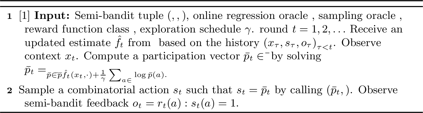
We propose an algorithm for the contextual combinatorial semi-bandit setting, called SquareCB.Comb(1), which achieves \(\iupboundlog{\sqrt{m A T \log\abs{\Fcal}}}\) regret under the realizability assumption. The algorithm is inspired by the SquareCB algorithm for contextual bandits [25], whose action-selection rule is the solution of a log-barrier regularized optimization problem [13] every round. At each round, the learner obtains an estimate of the reward function by calling a batch-mode online regression oracle \(\Ocal_{\mathrm{\small batch}}\) trained on past observations of the form (context, arms, rewards) (line [line:sqcomb-regression]), and observes the context \(x_t\) (line [line:sqcomb-context]). The learner then computes a participation vector \(\bar{p}_t\) over arms by solving a log-barrier regularized optimization problem (line [line:sqcomb-logbarrier]), and invokes a sampling oracle \(\Ocal_{\mathrm{\small sample}}\) to sample a combinatorial action \(s_t\) whose marginals match \(\bar{p}_t\) (line [line:sqcomb-sampling]). Finally, the learner observes the semi-bandit feedback \(o_t\) (line [line:sqcomb-feedback]) and forwards the new observation to \(\Ocal_{\mathrm{\small batch}}\) for use in the next round.
4.0.0.1 Computing an exploratory participation vector.
Our key algorithmic innovation lies in the computation of the participation vector \(\bar{p}_t\): at that step, the learner solves the following \(A\)-dimensional convex optimization problem (Eq. [eqn:log-barrier]). The first term in the objective, \(\iinner{\bar{p}}{\hat{f}_t(x_t,\cdot)}\), measures the “greediness” of the participation vector \(\bar{p}\), i.e., how optimal \(\bar{p}\) is with respect to the current reward function estimate \(\hat{f}_t\) and context \(x_t\); the second term \(\frac{1}{\gamma}\sum_{a \in \Acal}\log\bar{p}(a)\) is a log-barrier regularizer that encourages \(\bar{p}\) to spread its support, thereby preventing concentration on a small set of arms and promoting exploration. By balancing these two terms, the learner obtains a participation vector that exploits the current reward estimate while ensuring sufficient exploration to control the estimation error.
4.0.0.2 Sampling Oracle for Combinatorial Constraints.
The learner needs to sample a combinatorial action \(s_t\) from a distribution \(p_t \in \Delta(\Scal)\) whose marginal expectation matches the participation vector \(\bar{p}_t\) computed in Line [line:sqcomb-logbarrier]. This step is nontrivial because the participation vector \(\bar{p}_t\) is defined in the convex hull of the combinatorial action space \(\bar\Scal\), whose dimension is \(A\), while the actual sampling must be performed in \(\Delta(\Scal)\), a space of dimension \(\abs{\Scal}\) that can be exponentially larger than \(A\). For many structured combinatorial action sets, however, efficient sampling algorithms are readily available. For instance:
Unordered \(m\)-set recommendations with \(n\) items. Here, after computing \(\bar{p}_t\), we can use dependent rounding [32] to sample \(s_t\) with running time \(O(n)\).
Ordered \(m\)-slate recommendations with \(n\) items. [8] give an efficient sampler (which in turn uses the efficient algorithm of [33]) that first decomposes any \(\bar{p} \in \bar{\Scal}\) to a convex combination of \(n^2\) matrices, and samples from it.
Contextual shortest path on DAG. Any \(\bar{p} \in \bar{\Scal}\) is a unit \(s\)-\(t\) flow, and can be represented as a convex combination of \(s\)-\(t\) paths via standard flow decomposition procedures [34].
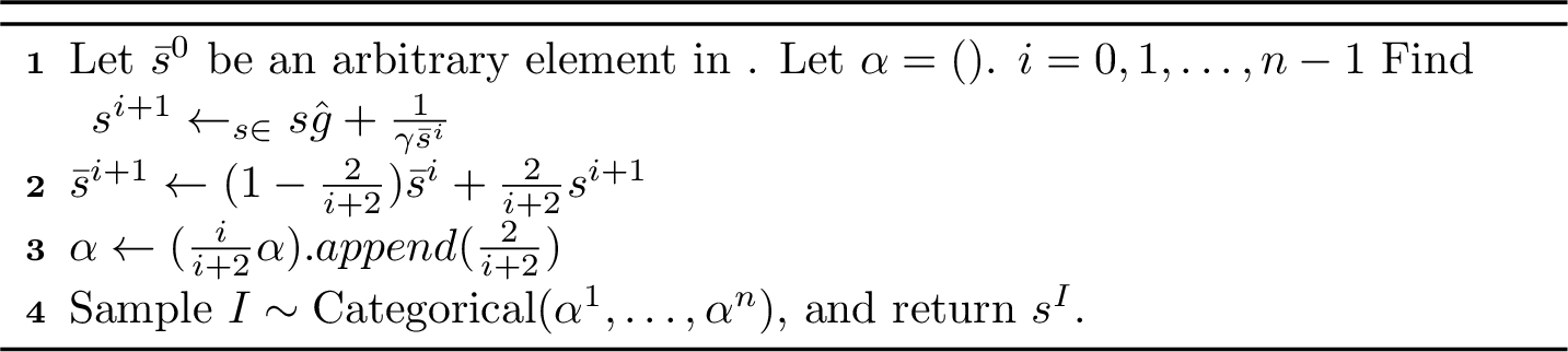
When \(\Scal\) admits an efficient linear optimization oracle (i.e., \(\argmin_{s \in \Scal} \inner{\ell}{s}\) is tractable for any \(\ell\)), as in shortest path and maximum weight matching, lines [line:sqcomb-logbarrier] and [line:sqcomb-sampling] can be merged: Frank-Wolfe on Eq. [eqn:log-barrier] produces iterates \(\bar{p}_n = \sum_{i=1}^n \alpha^i s^i\) with \(s^i \in \Scal\) and \(\alpha \in \Delta^{n-1}\), so sampling \(i \sim \mathrm{Categorical}(\alpha)\) and returning \(s^i\) yields \(s_t\) with marginals \(\bar{p}_n\). See 3 in Appendix 9.
4.1 Regret Analysis of SquareCB.Comb↩︎
We now present the main regret guarantee of SquareCB.Comb. In 1, we give a general regret bound in terms of the online regression oracle’s square-loss regret \(\mathrm{Reg}_{\mathrm{batch}}(T)\), which, combined with the guarantee of [assum:online-reg-semi], yields the explicit bound in 1.
Theorem 1 (Total regret bound). Suppose [assum:realizable,assum:action-size] hold and SquareCB.Combuses the constant exploration parameter \(\gamma = \sqrt{A T / \mathrm{Reg}_{\mathrm{batch}}(T)}\). Then the expected regret of SquareCB.Combis bounded as \[\EE\sbr{\Regret(T)} \leq \Ocal\del{\sqrt{A\,T\,\mathrm{Reg}_{\mathrm{batch}}(T)}}.\]
Combining 1 with the guarantee of the online regression oracle in the finite-class semi-bandit setting gives the following regret bound:
Corollary 1. Under [assum:realizable,assum:action-size,assum:online-reg-semi], and \(\gamma = \sqrt{\frac{A T}{m \log \abs{\Fcal}}}\), the expected regret of SquareCB.Combis upper bounded by \[\EE\sbr{\Regret(T)} \leq \Ocal\del{\sqrt{m A T \log |\Fcal|}}.\]
The bound is sublinear in \(T\) and exhibits the same \(\sqrt{mAT}\) dependence as the standard regret rate for the stochastic combinatorial semi-bandit problem under linear rewards [27], while permitting the mean reward function to belong to a general class \(\Fcal\). When \(m=1\), the contextual combinatorial semi-bandit setting reduces to the standard contextual bandit setting, and 1 recovers the \(\sqrt{A T \log\abs{\Fcal}}\) regret of the IGW algorithm for contextual bandits [25] under realizability. Compared with reducing CCSB to a contextual bandit problem on the slate space and applying a contextual bandit algorithm to the aggregated full-bandit reward, SquareCB.Comb’s regret bound scales as \(\sqrt{m A T \log\abs{\Fcal}}\) rather than \(m\sqrt{A T \log\abs{\Fcal}}\) (see 12 for a formal justification); this gap can be significant when \(m\) is large.
Specializing 1 to the three running examples gives:
Unordered \(m\)-set with \(n\) items. Each arm corresponds to one of the \(n\) items, so \(A = n\), and 1 yields regret \(\iupboundlog{\sqrt{m n T \log\abs{\Fcal}}}\). This matches the \(\iupboundlog{\sqrt{m n T \log\abs{\Pi}}}\) regret of [8], [19], which compete against the best policy in a class \(\Pi\), while SquareCB.Combis computationally more efficient since it relies on a better practicality of regression oracles relative to classification oracles.
Ordered \(m\)-slate with \(n\) items. Since \(A = m n\), 1 yields regret \(\iupboundlog{m\sqrt{n T \log\abs{\Fcal}}}\), comparable to the bound of [8] with better computational efficiency.
Contextual shortest path on a DAG. Since \(A = M\) and \(m \le N\), 1 yields regret \(\iupboundlog{\sqrt{N M T \log\abs{\Fcal}}}\). In comparison, applying the contextual MDP algorithm of [17] requires solving an \(N\)-state, \(N\)-action MDP with episode length \(H=N\), which yields regret at least \(\iupboundlog{\sqrt{N^7 T \log\abs{\Fcal}}}\).
4.1.0.1 Extensions: infinite classes, misspecified setting, and offline oracle-efficient algorithm.
1 treats the regression oracle abstractly through its cumulative square-loss regret \(\mathrm{Reg}_{\mathrm{batch}}(T)\), which readily yields regret-efficient CCSB algorithms beyond the basic realizable, finite-class setting by plugging in different online regression oracles. For an infinite class \(\Fcal\), instantiating the oracle with online square-loss regression based on sequential covering or sequential Rademacher complexity [31], [35] replaces \(m\log\abs{\Fcal}\) with the corresponding sequential complexity. For the \(\varepsilon\)-misspecified setting, where \(\inf_{f \in \Fcal}\sup_{x,a}\abs{f(x,a)-f^\star(x,a)} \le \varepsilon\), combining SquareCB.Combwith the misspecification-aware online regression oracle of [13] yields regret \(\iupbound{\sqrt{mAT\log\abs{\Fcal}} + \varepsilon m \sqrt{A} T}\); the additive \(\varepsilon T\) factor is unavoidable in light of the \(\Omega(\varepsilon\sqrt{d}T)\) lower bound of [26] for the misspecified \(d\)-dimensional linear bandit problem. In 11, we present a variant of SquareCB.Combthat reduces CCSB to \(O(\log T)\) offline regression problems while enjoying similar regret guarantees when the contexts are i.i.d.Given the wider availability of offline regression guarantees, this variant can be preferable in practice [36].
4.2 Proof sketch of 1↩︎
In this section, we provide a proof sketch of 1. We aim to adopt an analysis similar to SquareCB [25] that first bounds the instantaneous regret at round \(t\) in terms of the expected regression error at the same round, and then conclude the regret bound by summing over all \(t\)’s. However, SquareCB’s analysis is inherently tied to bandit feedback (the learner receives a single reward observation per round) and thus does not extend to our semi-bandit setting. Furthermore, the general E2D algorithm [12] (see 7 for a brief overview of the DMSO framework and the Decision-Estimation Coefficient) is not directly applicable here, since we do not have exact knowledge of the conditional distribution of \(\cbr{r_t(a): s_t(a) = 1}\) given the reward model \(f\) and \((x_t, s_t)\). This inspires us to define a new notion of DEC customized to square loss and combinatorial semi-bandits:
Definition 1. For a regressor \(\hat{g}: \Acal \to [0,1]\), a function class \(\Gcal\), and a combinatorial action set \(\Scal\), define their combinatorial square-loss DEC (CS-DEC) as \[\mathsf{dec}_\gamma(\hat{g}, \Gcal) = \min_{p \in \Delta(\Scal)} \underbrace{ \max_{q \in \Delta(\Scal), g^\star \in \Gcal} \EE_{s \sim q} \sbr{\inner{g^\star}{s}} - \EE_{s \sim p} \sbr{\inner{g^\star}{s}} - \gamma \EE_{s \sim p} \sbr{ \sum_{a =1}^A s(a) (\hat{g}(a) - g^\star(a))^2 } }_{ =: F(p)} , \label{eqn:dec-distn}\qquad{(1)}\] and define \(\mathsf{dec}_\gamma(\Gcal) = \max_{\hat{g}} \mathsf{dec}_\gamma(\hat{g}, \Gcal)\).
The CS-DEC accounts for the semi-bandit feedback by offsetting the instantaneous regret with the expected square-loss regression error over the entire set of arms associated with the combinatorial action; unlike DEC, it does not rely on exact probabilistic modeling of the reward distribution. To use CS-DEC for algorithm design, we need to find a distribution \(p \in \Delta(\Scal)\) that approximately minimizes \(F(\cdot)\). This is in general difficult, since the corresponding optimization problem is \(|\Scal|\)-dimensional and \(|\Scal|\) may be exponential in \(m\). Our key observation is that the CS-DEC admits an equivalent representation in the space of participation vectors, which has the much lower dimension \(A\), thereby admitting tractable solutions:
We have the following equivalent characterization: \[\mathsf{dec}_\gamma(\hat{g}, \Gcal) = \min_{\bar{p} \in \bar{\Scal}} \underbrace{ \max_{\bar{q} \in \bar{\Scal}, g^\star \in \Gcal} \inner{g^\star}{\bar{q}} - \inner{g^\star}{\bar{p}} - \gamma \sum_{a=1}^A \bar{p}(a) (\hat{g}(a) - g^\star(a))^2. }_{ =: \bar{F}(\bar p)} \label{eqn:dec-part}\tag{2}\] In addition, any \(p\) such that \(\EE_{s \sim p}\sbr{s} = \bar{p}\) satisfies that \(F(p) = \bar{F}(\bar p)\).
This enables the optimization problem ?? to be approximately solved in two steps: first, compute a \(\bar{p}\) that approximately solves 2 ; second, convert \(\bar{p}\) into a distribution \(p \in \Delta(\Scal)\) satisfying \(\EE_{s \sim p}[s] = \bar{p}\).
We show that the solution to the optimization problem in line [line:sqcomb-logbarrier] certifies that \(\mathsf{dec}_\gamma( \hat{f}_t(x_t, \cdot), \Fcal_{x_t} ) \leq \frac{A}{\gamma}\), where \(\Fcal_{x_t} := \cbr{f(x_t, \cdot): f \in \Fcal}\). To this end, we design a surrogate min-max objective that relaxes the DEC, and establish two intermediate results: (i) the participation vector computed by the log-barrier optimization certifies a small value of the surrogate min-max objective; and (ii) a small value of the surrogate objective certifies a small value of the DEC.
Specifically, our surrogate objective is: \[\begin{align} \inf_{\bar{p} \in \bar{\Scal}} \max_{\bar{q} \in \bar{\Scal}} \inner{\hat{f}_t(x_t,\cdot)}{\bar q} - \inner{\hat{f}_t(x_t,\cdot)}{\bar p} + \frac{1}{\gamma}\mathsf{Coverage}(\bar p, \bar q). \label{eqn:doec} \end{align}\tag{3}\] where \(\mathsf{Coverage}(\bar p, \bar q) = \sum_{a \in \Acal} \frac{\bar q(a)^2}{\bar p(a)}\) quantifies the estimation error under the data collected using action distributions with participation vector \(\bar p\) when trying to estimate the reward of action distribution with participation vector \(\bar q\). In 1, we show that the \(\bar{p}_t\) computed by the log-barrier optimization certifies a small value of the above surrogate objective. Subsequently, in 2, we show that any participation vector \(\bar{p}_t\) that certifies the surrogate min-max objective to be smaller than \(A / \gamma\) also certifies the DEC to be smaller than \(O(A/\gamma)\).
Combining the above two lemmas yields the instantaneous regret decomposition: \[\begin{align} \max_{s \in \Scal} \inner{s}{f^\star(x_t,\cdot)} - \inner{\bar{p}_t}{f^\star(x_t,\cdot)} \lesssim \frac{A}{\gamma} + \gamma \opnorm{\hat{f}_t(x_t,\cdot)-f^\star(x_t,\cdot)}{\bar{p}_t}^2. \end{align}\] By taking the instantaneous regret decomposition at each round and summing over \(t\), we have \[\begin{align} \sum_{t=1}^T \max_{s \in \Scal} \inner{s}{f^\star(x_t,\cdot)} - \sum_{t=1}^T \inner{\bar{p}_t}{f^\star(x_t,\cdot)} &\lesssim \frac{A T}{\gamma} + \gamma \sum_{t=1}^T \opnorm{\hat{f}_t(x_t,\cdot)-f^\star(x_t,\cdot)}{\bar{p}_t}^2 \\ &\leq \frac{A T}{\gamma} + \gamma \mathrm{Reg}_{\mathrm{batch}}(T). \end{align}\] Here, the second inequality is due to the batch-mode online regression oracle’s guarantee as well as that \(\EE\sbr{y_t(a) \mid x_t} = f^\star(x_t, a)\) for all \(a \in \Acal\). Finally, taking expectation over the randomness in the algorithm and history, choosing \(\gamma=\sqrt{AT/\mathrm{Reg}_{\mathrm{batch}}(T)}\) yields the regret guarantee of 1: \[\EE\sbr{\Regret(T)} \lesssim \sqrt{A T \mathrm{Reg}_{\mathrm{batch}}(T)}.\] Under [assum:online-reg-semi], substituting \(\mathrm{Reg}_{\mathrm{batch}}(T)=m\log\abs{\Fcal}\) recovers the result in 1.
5 Lower Bound↩︎
We complement the upper bound of 1 with a matching lower bound, showing that SquareCB.Combis minimax optimal in \(m\), \(A\), \(T\), and \(\log\abs{\Fcal}\) up to logarithmic factors. The lower bound is parameterized by an upper bound \(N\) on the size of the reward function class \(\Fcal\) used in the construction.
theoremlowerBoundCCSB For any \(m, A, T, N \in \NN\) such that \(A/m \in \NN\), \(N \geq A/m\), \(T / \lfloor \log_{A/m} N \rfloor \in \NN\), and \(T / \lfloor \log_{A/m} N \rfloor \geq 16 A / m\), there exists a CCSB problem with \(A\) arms and combinatorial-action size at most \(m\), and a reward function class \(\Fcal\) with \(\abs{\Fcal} \leq N\), such that for any algorithm \(\mathrm{Alg}\) there is an environment realizable with respect to \(\Fcal\) on which the expected regret of \(\mathrm{Alg}\) is at least \(\ilowboundlog{\sqrt{m\,A\,T \log N}}\).
The construction (deferred to 14) partitions the horizon into \(M = \lfloor \log_{A/m} N \rfloor\) equal-length intervals, assigns each interval a distinct context, and embeds an independent non-contextual \(m\)-path instance of [27] into each interval. Aggregating the per-interval \(\ilowbound{\sqrt{m A T / M}}\) regret across the \(M\) intervals yields the displayed bound.
5.0.0.1 Minimax optimality.
Setting \(N = \abs{\Fcal}\) in [thm:lower-bound-ccsb] yields a lower bound of \(\ilowboundlog{\sqrt{m\,A\,T \log\abs{\Fcal}}}\), which matches the upper bound of 1 up to polylogarithmic factors. Hence SquareCB.Combattains the minimax-optimal regret rate for CCSB with general reward function approximation up to logarithmic factors. To our knowledge, this is the first minimax-optimal regret guarantee for CCSB beyond the linear-reward setting. We also remark that our lower bound crucially uses the dependence of \((r_t(a))_{a \in \Acal}\). Under the additional assumption that \((r_t(a))_{a \in \Acal}\) are independent given \(x_t\) (as studied in [37]), we conjecture that the minimax regret bound may be strictly lower than \(\iupboundlog{\sqrt{m\,A\,T \log\abs{\Fcal}}}\); we leave this as an interesting open question.
6 Experiments↩︎
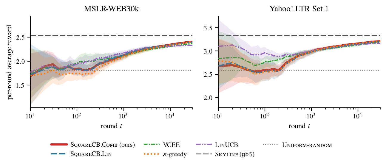
We compare SquareCB.Combagainst several semi-bandit and contextual-bandit baselines on two public learning-to-rank corpora, running each algorithm for a single pass over the entire corpus, so that the horizon \(T\) equals the corpus size. We first search an optimal hyperparameter for each algorithm by maximizing the mean realized cumulative reward over the tuning seeds, then choose the best hyperparameter for each algorithm and compare their performance on \(10\) disjoint runs.
6.0.0.1 Datasets.
We use MSLR-WEB30k [38] and the Yahoo!Learning-to-Rank Challenge Set 1 [39]. Both corpora are recast as CCSB instances via the standard supervised-to-bandit reduction [9], [19], [25], with per-document relevance labels in \(\{0,1,2,3,4\}\) used as semi-bandit feedback. Following the conventions of [19], we set the candidate pool size \(A = 10\) and the slate size \(m = 3\) on MSLR-WEB30k, and \(A = 6\), \(m = 2\) on Yahoo!LTR Set 1. After filtering out queries with fewer than \(A\) candidate documents, each run makes one pass over the remaining queries, giving horizons of \(T = 30{,}846\) rounds on MSLR-WEB30k and \(T = 27{,}630\) rounds on Yahoo!LTR Set 1 (see 13 for details).
6.0.0.2 Algorithms.
We instantiate SquareCB.Comb(1) with a linear regression (lin) and a gradient-boosted regression tree ensemble (gb; see Appendix 13.3 for details) as its regression oracle. We compare against four other algorithms: SquareCB.Lin [13], which replaces the per-arm IGW sampler with a log-determinant optimization problem over the \(\binom{A}{m}\) size-\(m\)
super-arms, drawing the slate as one categorical sample from the resulting distribution and uses the summed semi-bandit reward feedback as bandit reward feedback; VCEE [19], the policy-based contextual combinatorial bandit algorithm; LinUCB [40], the linear UCB algorithm adapted to the semi-bandit setting; and \(\varepsilon\)-greedy [41], which maintains an online regression oracle of per-arm rewards and, at each round, plays a uniformly random size-\(m\)
slate with probability \(\varepsilon\) or the predicted top-\(m\) slate under the oracle otherwise. We additionally report two non-learning algorithms for reference: a uniform-random slate
(the floor), and a supervised skyline (the ceiling) that fits a regression oracle once on the entire labeled corpus and then greedily plays the in-sample top-\(m\) arms every round; the table (2) reports one skyline per regression oracle (lin, gb2, gb5).
6.0.0.3 Results.
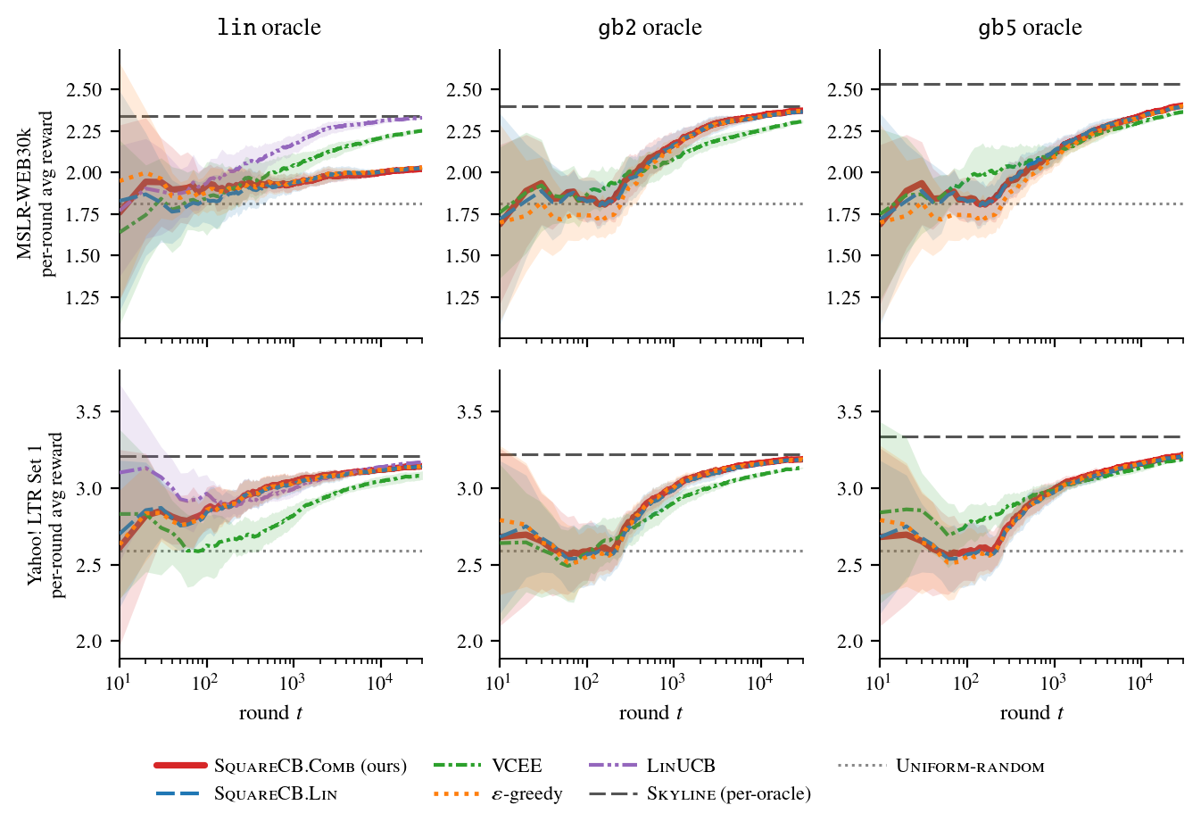
2 plots the per-round average reward (on a logarithmic round axis) and 2 reports its value at the final round \(t = T\), both over the \(10\) disjoint Stage-2 seeds: the figure shades a \(\pm 1\) standard-deviation band across the \(10\) seeds, while the table reports the mean \(\pm\) standard error (\(\mathrm{std}/\sqrt{10}\)).
| MSLR-WEB30k | Yahoo!LTR Set 1 | |||||
|---|---|---|---|---|---|---|
| 2-4(lr)5-7 Algorithm | lin | gb2 | gb5 | lin | gb2 | gb5 |
| Skyline | \(2.340 \pm 0.001\) | \(2.402 \pm 0.001\) | \(2.536 \pm 0.001\) | \(3.209 \pm 0.001\) | \(3.219 \pm 0.001\) | \(3.335 \pm 0.001\) |
| (ours) | \(2.024 \pm 0.002\) | \(\mathbf{2.373 \pm 0.002}\) | \(\mathbf{2.404 \pm 0.001}\) | \(3.141 \pm 0.001\) | \(\mathbf{3.187 \pm 0.001}\) | \(\mathbf{3.217 \pm 0.001}\) |
| SquareCB.Lin | \(2.028 \pm 0.002\) | \(2.366 \pm 0.002\) | \(2.398 \pm 0.002\) | \(3.138 \pm 0.001\) | \(3.184 \pm 0.001\) | \(3.211 \pm 0.001\) |
| VCEE | \(2.252 \pm 0.002\) | \(2.309 \pm 0.003\) | \(2.366 \pm 0.003\) | \(3.083 \pm 0.009\) | \(3.132 \pm 0.001\) | \(3.189 \pm 0.002\) |
| \(\varepsilon\)-greedy | \(2.030 \pm 0.002\) | \(2.373 \pm 0.001\) | \(2.401 \pm 0.002\) | \(3.140 \pm 0.001\) | \(3.186 \pm 0.001\) | \(3.214 \pm 0.001\) |
| LinUCB | \(\mathbf{2.330 \pm 0.002}\) | — | — | \(\mathbf{3.168 \pm 0.001}\) | — | — |
| Uniform-random | \(1.815 \pm 0.002\) | \(2.591 \pm 0.002\) | ||||
3pt
7 Decision Making with Structured Observations↩︎
[12] introduced a general framework for interactive decision making with structured observations (DMSO), which captures a wide range of problems including contextual bandits and reinforcement learning, and which subsumes the contextual combinatorial semi-bandit setting. The interactive protocol of DMSO is as follows. At the beginning, the learner has access to a model class \(\Mcal\) that contains the true model \(M^\star\); each model \(M\) is associated with a reward function \(f^M: \Pi \to \RR\). At every time step \(t\):
The learner selects a decision \(\pi_t\) from a decision set \(\Pi\);
The environment draws an observation \(o_t \sim M^\star(\pi_t)\) and sends it to the learner; the learner incurs reward \(f^{M^\star}(\pi_t)\).
The exploration-exploitation trade-off is a fundamental challenge in DMSO, and a key step in our analysis is to characterize its statistical complexity. The Decision-Estimation Coefficient (DEC) of [12] captures this complexity: \[\mathsf{dec}_\gamma(\Mcal, \hat{M}) \mathrel{\vcenter{:}}= \inf_{p \in \Delta(\Pi)} \sup_{q \in \Delta(\Pi),\, M^\star \in \Mcal} \EE_{\pi \sim q} \sbr{ f^{M^\star}(\pi) } - \EE_{\pi \sim p} \sbr{ f^{M^\star}(\pi) } - \gamma \EE_{\pi \sim p} \sbr{ D_H^2 (\hat{M}(\pi), M^\star(\pi)) },\] where \(D_H^2\) is the squared Hellinger distance between the distributions over observations induced by \(\pi\) under \(M\) and \(\hat{M}\).
8 Additional Related Work↩︎
8.0.0.1 Noncontextual combinatorial semi-bandit: stochastic and adversarial settings.
The non-contextual combinatorial semi-bandit, also known as the combinatorial multi-armed bandit (CMAB), is a special case of the CCSB problem in which no contextual information is available. The CMAB problem admits a variety of formulations in the literature [42]. [43] first studied a special case of the CMAB problem under the fixed-cardinality constraint, in which the learner chooses \(m\) arms per round, and proposed an algorithm with an asymptotically optimal regret guarantee. [6] studied the CMAB problem with arbitrary combinatorial constraints on the action space and proposed a UCB-based algorithm with an \(\iupboundlog{m^3 A/\Delta^2}\) instance-dependent bound, where \(\Delta\) is the minimum gap between the optimal and a suboptimal combinatorial action; [27] analyzed a similar UCB-based algorithm and improved the instance-dependent bound to \(\iupboundlog{m A/\Delta}\) to achieve optimality when the arm set has dependency and obtained a \(\iupbound{\sqrt{m A T}}\) minimax regret bound. [37] gives an optimal instance-dependent rate as \(\iupboundlog{\sqrt{m} A/\Delta}\) when arms are independent. [44] extended the analysis to a general reward structure of a combinatorial action and gave both gap-dependent and gap-independent regret bounds. [45] studied the pure-exploration / best-arm identification problem with fixed confidence in the CMAB setting, where the learner aims to identify the optimal combinatorial action with high confidence.
Another line of work studies the CMAB problem in the adversarial setting with semi-bandit feedback, where each arm’s reward is chosen by an adversary. [8] first studied the CMAB problem under the fixed-cardinality constraint and proposed an algorithm based on relative-entropy projections over the set of distributions on slates, achieving \(\iupbound{\sqrt{m A T}}\) regret. [46] adapted the Online Stochastic Mirror Descent (OSMD) algorithm to solve the adversarial CMAB problem and obtained optimal minimax regret bounds \(\iupbound{\sqrt{m A T}}\); [47] proposed an FTRL-based algorithm that achieves the first best-of-both-worlds guarantee, with \(\iupbound{\sqrt{T}}\) regret in the adversarial setting and \(\iupbound{\log T}\) regret in the stochastic setting;
8.0.0.2 Complexity measures of online decision-making problems.
Our method follows the Estimation-to-Decisions (E2D) paradigm of [12], which reduces an online decision-making problem to a statistical estimation problem. [12] introduced the Decision-Estimation Coefficient (DEC) as a complexity measure for the interactive decision-making problems and developed the Decision Making with Structured Observations (DMSO) framework around it. This framework has inspired a line of work that follows the same reduction idea. For example, [48] extended the DEC to adversarial decision-making with structured observations; [49] bridged the Bayesian theory of information-directed sampling and the frequentist theory of E2D via the DEC; and [50] relaxed E2D to an anytime variant and applied it to linear bandits with side observations.
9 Sampling from exploration distribution using linear optimization oracle↩︎
Recall that a key step of Algorithm 1 is to sample \(s \in \Scal\) at random such that \(\EE[s]\) is the solution of the following optimization problem: \[\max_{\bar{s} \in \bar{S}} \inner{g}{\bar{s}} + \frac{1}{\gamma} \sum_{a=1}^A \log(\bar{s}(a)) \label{eqn:log-barrier-abstract}\tag{4}\] We show in this section that as long as \(\Scal\) admits an efficient linear optimization oracle, this can be done efficiently. Indeed, Algorithm 3 first solves the optimization above approximately using the Frank-Wolfe algorithm [51], which crucially maintains a sparse convex combination representation of the iterates \(\bar{s}^i\)’s – specifically, at any point, \(\bar{s}^i = \sum_{j=1}^i \alpha_j s^j\), where \(\alpha \in \Delta^{i-1}\) and all \(s^j\)’s are elements in \(\Scal\). Specifically, the last iterate, \(\bar{s}^n\), is also a convex combination of \(s^i, i=1,\ldots,n\). Thus, sampling \(I = i\) with probability \(\alpha^i\) and returning \(s^I\) that has expectation equal to \(\bar{s}^n\), an approximate solution to 4 .
10 Regret Guarantees of SquareCB.comb↩︎
In this section, we present and prove the regret guarantee of SquareCB.Comb, and provide all necessary lemmas with their proofs in the following subsection.
10.1 Lemmas about the reduction from DEC to the log-barrier optimization↩︎
The analysis in this subsection is conducted conditional on the observed context \(x_t\) and the estimated reward function \(\hat{f}_t\) at round \(t\), and we omit the dependence on \(x_t\) and \(\hat{f}_t\) for brevity. We write \(g(a)\), \(\hat{g}(a)\), and \(\Gcal\) to denote \(f^\star(x_t, a)\), \(\hat{f}_t(x_t, a)\), and \(\Fcal_{x_t} := \cbr{ f(x_t, \cdot): f \in \Fcal }\), respectively. In the proof sketch of 1, we noted that the solution of the log-barrier optimization problem in Eq. [eqn:log-barrier] certifies that the CS-DEC is upper bounded by \(\frac{A}{\gamma}\) up to a constant factor. \[\begin{align} \bar{p}_t = \arg \max_{\bar{q} \in \bar{\Scal}} \inner{\hat{g}}{\bar{q}} + \frac{1}{\gamma} \sum_{a \in \Acal} \log(\bar{q}(a)) \end{align}\] Specifically, we aim to show that the solution \(\bar{p}_t\) satisfies the following inequality: \[\begin{align} \max_{\bar{q} \in \bar{\Scal}, g^\star} \inner{g^\star}{\bar{q}} - \inner{g^\star}{\bar{p}_t} - \gamma \cdot \opnorm{g^\star - \hat{g}}{\bar{p}_t}^2 \lesssim \frac{A}{\gamma}, \label{eqn:small-dec} \end{align}\tag{5}\] To this end, we introduce a surrogate min-max optimization problem that connects the log-barrier optimization problem with Eq. 5 . Specifically, the surrogate min-max optimization problem is defined as follows: \[\begin{align} \min_{\bar{p} \in \bar{\Scal}} \max_{\bar{q} \in \bar{\Scal}} \inner{\hat{g}}{\bar{q}} - \inner{\hat{g}}{\bar{p}} + \frac{1}{\gamma} \mathsf{Coverage}(\bar{p}, \bar{q}) \label{eqn:small-doec} \end{align}\tag{6}\] where the coverage term is defined as \(\mathsf{Coverage}(\bar{p}, \bar{q}) = \sum_{a \in \Acal} \frac{\bar{q}(a)^2}{\bar{p}(a)}\). We show in 1 that the solution \(\bar{p}_t\) of the log-barrier optimization problem approximately solves Eq. 6 . Taking Eq. 6 as an intermediate result, we then show in 2 that \(\bar{p}_t\) certifies a small CS-DEC value (Eq. 5 ).
Lemma 1 (Solving log-barrier regularized problem approximately solves Eq. 6 ). For any \(\hat{g}\) , define \[\Lcal(\bar{s}; \hat{g}) := \inner{\hat{g}}{\bar{s}} + \frac{1}{\gamma} \sum_{a \in \Acal} \log(\bar{s}(a))\] for any \(\bar{s} \in \bar{\Scal}\). Let \(\hat{p}\) be the optimal solution of \(\max_{\bar{s} \in \bar{S}} \Lcal(\bar{s}; \hat{g})\), then we have \[\max_{\bar{q} \in \bar{\Scal}} \inner{\hat{g}}{\bar{q}} - \inner{\hat{g}}{\hat{p}} + \frac{1}{\gamma} \mathsf{Coverage}(\hat{p}, \bar{q}) \leq \frac{A}{\gamma}.\]
Proof of 1. Throughout this proof, for any vector \(u \in \RR^{A}\) with strictly positive entries, we write \(\frac{1}{u} \in \RR^{A}\) for its entrywise reciprocal, and \(u^2 \in \RR^A\) for its entrywise square.
Since \(\Lcal(\bar{q}; g)\) is a strictly concave function of \(\bar{q}\) and \(\bar{\Scal}\) is a convex set, we know that the optimal solution \(\hat{p}\) is achieved when it meets the first-order optimality condition, that is, for any \(\bar{q} \in \bar{\Scal}\), we have \[\begin{align} \inner{\nabla_{\bar{q}} -\Lcal(\bar{q})\mid_{\bar{q}=\hat{p}}}{\bar{q} - \hat{p}} &\geq 0 \\ \Leftrightarrow \inner{-\hat{g} - \frac{1}{\gamma \hat{p}}}{\bar{q} - \hat{p}} &\geq 0 } \\ \Leftrightarrow \inner{\hat{g} + \frac{1}{\gamma \hat{p}}}{\bar{q} - \hat{p}} &\leq 0 \\ \Leftrightarrow \inner{\hat{g}}{\bar{q} - \hat{p}} + \frac{1}{\gamma} \inner{\frac{1}{\hat{p}}}{\bar{q}} &\leq \frac{A}{\gamma} \end{align}\]
Since \(\hat{p}\) satisfies the above first-order optimality condition, we know that for any \(\bar{q} \in \bar{\Scal}\), \[\begin{align} \inner{\hat{g}}{\bar{q} - \hat{p}} + \frac{1}{\gamma} \inner{\frac{1}{\hat{p}}}{\bar{q}} &\leq \frac{A}{\gamma} \nonumber \\ \Rightarrow \inner{\hat{g}}{\bar{q}} - \inner{\hat{g}}{\hat{p}} + \frac{1}{\gamma} \inner{\frac{1}{\hat{p}}}{\bar{q}^2} &\leq \frac{A}{\gamma} \nonumber \\ \Leftrightarrow \inner{\hat{g}}{\bar{q}} - \inner{\hat{g}}{\hat{p}} + \frac{1}{\gamma} \mathsf{Coverage}(\hat{p}, \bar{q}) &\leq \frac{A}{\gamma} \label{eqn:log-barrier-optimality} \end{align}\tag{7}\] ◻
Lemma 2 (Certifying Eq. 5 by Eq. 6 ). Let \(\hat{g}\) be any reward estimate and \(\hat{p} \in \bar{\Scal}\) a participation vector. If \(\hat{p}\) satisfies the inequality \[\max_{\bar{q} \in \bar{\Scal}} \inner{\hat{g}}{\bar{q}} - \inner{\hat{g}}{\hat{p}} + \frac{1}{\gamma} \mathsf{Coverage}(\hat{p}, \bar{q}) \leq \frac{A}{\gamma},\] then \(\hat{p}\) also satisfies the inequality \[\max_{\bar{q} \in \bar{\Scal},\, g^\star} \inner{g^\star}{\bar{q}} - \inner{g^\star}{\hat{p}} - \gamma \cdot \opnorm{g^\star - \hat{g}}{\hat{p}}^{2} \lesssim \frac{A}{\gamma},\] where we recall that the squared weighted norm is defined as \(\opnorm{g^\star - \hat{g}}{\hat{p}}^{2} = \sum_{a \in \Acal} \hat{p}(a)\,\bigl(g^\star(a) - \hat{g}(a)\bigr)^{2}\).
Proof of 2. Fix the ground-truth reward function \(g^\star\) and two participation vectors \(\bar{s}, \hat{p} \in \bar{\Scal}\). Decompose the excess reward among \(\bar{s}\) and \(\hat{p}\) as follows: \[\begin{align} \inner{g^\star}{\bar{s}} - \inner{g^\star}{\hat{p}} = \inner{\hat{g}}{\bar{s}} - \inner{\hat{g}}{\hat{p}} + \inner{g^\star - \hat{g}}{\bar{s}} + \inner{\hat{g} - g^\star}{\hat{p}} \end{align}\] We bound the second difference by using the Off-policy evaluation (OPE) lemma (6) followed by AM-GM: \[\begin{align} \inner{g^\star - \hat{g}}{\bar{s}} &\leq \sqrt{ \mathsf{Coverage}(\hat{p}, \bar{s}) \cdot \opnorm{g^\star - \hat{g}}{\hat{p}}^2} \\ &\lesssim \frac{1}{\gamma} \mathsf{Coverage}(\hat{p}, \bar{s}) + \gamma \cdot \opnorm{g^\star- \hat{g}}{\hat{p}}^2. \end{align}\] For the third term, Cauchy-Schwarz combined with \(\sum_{a \in \Acal} \bar{s}(a) \leq m, \forall \bar{s} \in \bar{\Scal}\) from [assum:action-size] and AM-GM yields \[\begin{align} \inner{\hat{g} - g^\star}{\hat{p}} &\leq \sqrt{\idel{\sum_{a\in\Acal}\hat{p}(a)} \cdot \opnorm{\hat{g} - g^\star}{\hat{p}}^2} \\ &\leq \frac{m}{\gamma} + \frac{\gamma}{4} \cdot \opnorm{\hat{g} - g^\star}{\hat{p}}^2. \end{align}\] Plugging the two bounds back into the decomposition, \[\begin{align} \inner{g^\star}{\bar{s}} - \inner{g^\star}{\hat{p}} \lesssim \inner{\hat{g}}{\bar{s}} - \inner{\hat{g}}{\hat{p}} + \frac{1}{\gamma} \mathsf{Coverage}(\hat{p}, \bar{s}) + \frac{m}{\gamma} + \gamma \cdot \opnorm{g^\star - \hat{g}}{\hat{p}}^2. \end{align}\] Since the above inequality holds for any \(\bar{s} \in \bar{\Scal}\), we can take the maximum over \(\bar{s}\) on the left-hand side and use the fact that \(\hat{p}\) approximately solves Eq. 6 to upper bound the sum of first three terms on the right-hand side by \(\frac{A}{\gamma}\), which gives \[\begin{align} \inner{g^\star}{\bar{s}} - \inner{g^\star}{\hat{p}} &\lesssim \frac{A}{\gamma} + \frac{m}{\gamma} + \gamma \cdot \opnorm{g^\star - \hat{g}}{\hat{p}}^2 \\ \Rightarrow \inner{g^\star}{\bar{s}} - \inner{g^\star}{\hat{p}} - \gamma \cdot \opnorm{g^\star - \hat{g}}{\hat{p}}^2 &\lesssim \frac{A}{\gamma} \end{align}\] The last inequality holds for any \(\bar{s} \in \bar{\Scal}\) and \(g^\star \in \Gcal\), which completes the proof. ◻
Lemma 3 (Solution of log-barrier optimization certifies small DEC). Under [assum:realizable,assum:action-size], the solution \(\bar{p}_t\) of the log-barrier optimization problem in Eq. [eqn:log-barrier] satisfies that for any \(\bar{q} \in \bar{\Scal}\) and any \(g^\star \in \Gcal\), we have \[\begin{align} \inner{g^\star}{\bar{q}} - \inner{g^\star}{\bar{p}_t} - \gamma \cdot \opnorm{g^\star - \hat{g}}{\bar{p}_t}^2 \lesssim \frac{A}{\gamma}. \end{align}\]
Proof of 3. From 1, we have that the solution \(\bar{p}_t\) of the log-barrier optimization problem in Eq. [eqn:log-barrier] certifies Eq. 6 . Then, applying 2 by letting \(\hat{p} = \bar{p}_t\), we get that \(\bar{p}_t\) certifies Eq. 5 . ◻
10.2 Regret guarantee of SquareCB.Comb↩︎
We are now ready to bound the regret of SquareCB.Combat each round by leveraging the fact that the solution of the log-barrier optimization problem certifies a small DEC value. We define the regret of SquareCB.Combat round \(t\) as \(\regret_t(\bar{p}_t) = \max_{\bar{q} \in \bar{\Scal}} \inner{f^\star(x_t, \cdot)}{\bar{q}} - \inner{f^\star(x_t, \cdot)}{\bar{p}_t}\), which represents the difference between the expected reward of the best combinatorial action and that of the combinatorial action selected by SquareCB.Combat round \(t\).
Lemma 4 (Instantaneous regret upper bound of SquareCB.Comb). Under [assum:realizable,assum:action-size], for each round of the regret of SquareCB.Combis bounded by \[\begin{align} \regret_t(\bar{p}_t) \lesssim \frac{A}{\gamma} + \gamma \opnorm{f^\star(x_t, \cdot) - \hat{f}_t(x_t, \cdot)}{\bar{p}_t}^2. \end{align}\]
Proof of 4. By 3, the solution \(\bar{p}_t\) of the log-barrier optimization problem in Eq. [eqn:log-barrier] certifies that, for any \(\bar{q} \in \bar{\Scal}\) and any \(f^\star \in \Fcal\), \[\inner{f^\star(x_t, \cdot)}{\bar{q}} - \inner{f^\star(x_t, \cdot)}{\bar{p}_t} - \gamma \cdot \opnorm{f^\star(x_t, \cdot) - \hat{f}_t(x_t, \cdot)}{\bar{p}_t}^2 \lesssim \frac{A}{\gamma}.\] Then, for the regret of SquareCB.Combat round \(t\), we have \[\begin{align} &\quad \regret_t(\bar{p}_t) \\ &= \max_{\bar{q} \in \bar{\Scal}} \inner{f^\star(x_t, \cdot)}{\bar{q}} - \inner{f^\star(x_t, \cdot)}{\bar{p}_t} \\ &= \max_{\bar{q} \in \bar{\Scal}} \inner{f^\star(x_t, \cdot)}{\bar{q}} - \inner{f^\star(x_t, \cdot)}{\bar{p}_t} - \gamma \cdot \opnorm{f^\star(x_t, \cdot) - \hat{f}_t(x_t, \cdot)}{\bar{p}_t}^2 + \gamma \cdot \opnorm{f^\star(x_t, \cdot) - \hat{f}_t(x_t, \cdot)}{\bar{p}_t}^2 \\ &\leq \frac{A}{\gamma} + \gamma \cdot \opnorm{f^\star(x_t, \cdot) - \hat{f}_t(x_t, \cdot)}{\bar{p}_t}^2, \end{align}\] where the first inequality is due to Eq. 5 . ◻
We are now ready to prove the main regret guarantee of SquareCB.Comb.
Proof of 1. By 4, we bound the instantaneous regret of SquareCB.Combat every round \(t\). Summing over \(t = 1, \ldots, T\) and then taking expectation over all the randomness we have \[\begin{align} \EE[\Regret(T)] &= \sum_{t=1}^T \EE[\regret_t(\bar{p}_t)] \\ &\leq \sum_{t=1}^T \frac{A}{\gamma} + \gamma \cdot \EE[\opnorm{f^\star(x_t, \cdot) - \hat{f}_t(x_t, \cdot)}{\bar{p}_t}^2] } \\ &= \frac{T A}{\gamma} + \gamma \cdot \EE \sbr{ \EE_{s_t \sim p_t} \sbr{ \sum_{t=1}^T \sum_{a: s_t(a) = 1} \del{f^\star(x_t, a) - \hat{f}_t(x_t, a)}^2 } } \\ &\leq \frac{T A}{\gamma} + \gamma\, \mathrm{Reg}_{\mathrm{batch}}(T) \end{align}\] In the second-to-the-last equation, we use the definition of expectation. The last inequality uses the online regression guarantee in [assum:online-reg-semi], where for any sequence of \((s_t, a_t, o_t)_{t=1}^T\), we have \[\begin{align} & \EE\sbr{ \sum_{t=1}^T \sum_{a: s_t(a) = 1} (\hat{f}(x_t, a) - f^\star(x_t, a))^2 } \\ = & \EE\sbr{ \sum_{t=1}^T \sum_{a: s_t(a) = 1} \rbr{ (\hat{f}(x_t, a) - r_t(a))^2 - (f^\star(x_t, a) - r_t(a))^2 } } \\ \leq & \mathrm{Reg}_{\mathrm{batch}}(T), \end{align}\] where the equality is due to that \(\EE\sbr{r_t(a) \mid x_t } = f^\star(x_t, a)\).
Setting \(\gamma = \sqrt{A T / \mathrm{Reg}_{\mathrm{batch}}(T)}\) balances the dominant exploitation term \(T A/\gamma\) against the exploration penalty \(\gamma \mathrm{Reg}_{\mathrm{batch}}(T)\), yielding \(\Regret(T) \leq \Ocal\del{\sqrt{A T \mathrm{Reg}_{\mathrm{batch}}(T)}}\), which completes the proof. ◻
11 An Offline Oracle-efficient Variant: OE2D.Comb↩︎
In this section, we present OE2D.Comb, an epoch-based variant of SquareCB.Combthat replaces the batch-mode online regression oracle \(\Ocal_{\mathrm{\small batch}}\) with an offline regression oracle \(\Ocal_{\mathrm{\small batch.off}}\), in the spirit of the offline oracle-efficient contextual bandit algorithms FALCON [52] and the OE2D framework of [53]. The algorithm partitions the horizon \(T\) into \(M\) epochs with endpoints \(0 = \tau_0 < \tau_1 < \cdots < \tau_M = T\); within each epoch \(m\), the reward estimate \(\hat{f}_m \in \Fcal\) is held fixed, and at every round the same log-barrier optimization problem (the analogue of Eq. [eqn:log-barrier] with \(\gamma\) replaced by \(\gamma_m\)) is solved to obtain a participation vector \(\bar p_t \in \bar\Scal\). We assume access to an offline regression oracle \(\Ocal_{\mathrm{\small batch.off}}\) that, given a batch of i.i.d.semi-bandit observations, returns the empirical risk minimizer \(\hat{f}_m \in \Fcal\) of the squared loss summed over the observed coordinates; its on-policy estimation error is controlled by 8.
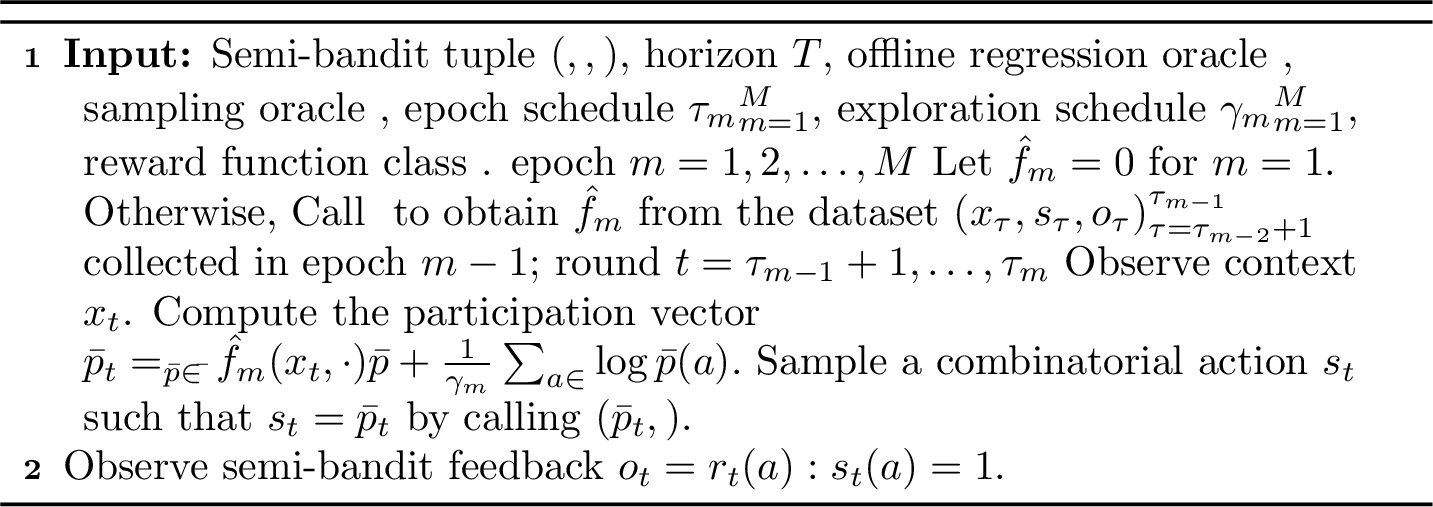
The optimization problem solved at every round of OE2D.Combis precisely the \(A\)-dimensional log-barrier optimization problem in SquareCB.Comb(Eq. [eqn:log-barrier]), instantiated with the per-epoch estimate \(\hat{f}_m\) and exploration parameter \(\gamma_m\). As in SquareCB.Comb, the convex hull constraint \(\bar p_t \in \bar\Scal\) ensures that \(\bar p_t\) is realizable by some distribution over \(\Scal\), and the sampling oracle \(\Ocal_{\mathrm{\small sample}}\) converts \(\bar p_t\) into a combinatorial action \(s_t\) with matching marginals (cf. [sec:reduction]). By 1, the resulting \(\bar p_t\) certifies the surrogate min-max objective of Eq. 3 at value at most \(A/\gamma_m\), which we use below to prove OE2D.Comb’s regret bound:
Theorem 2. Suppose that the contexts \(\cbr{x_t}_{t=1}^T\) are drawn i.i.d.from \(\Dcal_\Xcal\). Under [assum:realizable,assum:action-size], OE2D.Combwith the doubling schedule \(\tau_m = 2^m\) and exploration parameter \(\gamma_m = \sqrt{A / \mathrm{Reg}_{\Ocal_{\mathrm{\small batch.off}}}(\Fcal, \tau_{m-1}/2)}\) satisfies \[\begin{align} \EE\sbr{\Regret(T)} \leq \widetilde{\Ocal}\del{\sqrt{m\, A\, T \log\abs{\Fcal}}}. \end{align}\]
Proof sketch of 2. Our proof utilizes Theorem 3 (deferred after the proof), a regret theorem for an epoch-based decision making algorithm abstracted from [53]. First, we will adopt a policy-viewpoint of OE2D.Comb: at epoch \(m\), we view the algorithm as executing the policy \(\pi(x)\) with participation vector: \[\bar{\pi}_m(x) = \argmax_{\bar p \in \bar{\Scal}} \inner{\hat{f}_m(x, \cdot)}{\bar p} + \frac{1}{\gamma_m}\sum_{a \in \Acal} \log\del{\bar{p}(a)};\] Therefore, the regret of the algorithm can be represented as \[\EE\sbr{\Regret(T)} = \sum_{m=1}^M (\tau_m - \tau_{m-1}) \EE_{x \sim \Dcal_\Xcal} \sbr{ \max_{\lambda \in \Lambda} \inner{f^\star(x,\cdot)}{\lambda} - \inner{f^\star(x,\cdot)}{\pi_m(x)} }.\]
We now apply Theorem 3 by taking \(\Lambda = \bar{\Scal}\), \(p_m = \bar{\pi}_m\), \(C = \mathsf{Coverage}\) (recall that \(\mathsf{Coverage}(\bar{p}, \bar{q}) = \sum_{a=1}^A \frac{\bar{q}(a)^2}{\bar{p}(a)}\)), \(D_m = \frac{A}{\gamma_m}\) and \(E_m = \opnorm{\hat{f}_m - f^\star}{\bar{p}_{m-1}}^2\). The two conditions of Theorem 3 are satisfied:
Condition [item:p-m-doec] follows from Lemma 1;
Condition [item:ope] follows from Lemma 6;
Thus, applying the theorem, \[\begin{align} &\EE\sbr{\Regret(T)} \\ \leq & \EE\sbr{\tau_1 + \del{\max_{n \in [2, M]} \frac{\tau_n}{\gamma_n}} \del{A + \max_{n \in [2, M]} \gamma_n^2 \opnorm{\hat{f}_m - f^\star}{\bar{p}_{m-1}}^2 } } \\ \lesssim & \tau_1 + \rbr{ \max_{n \in [2,M]} \frac{\tau_n}{\gamma_n} }\cdot \rbr{ A + \max_{n \in [2,M]} \gamma_n^2 \mathrm{Reg}_{\Ocal_{\mathrm{\small batch.off}}}(\Fcal, \tau_{n-1}/2) } \\ \lesssim & 1 + \max_{n \in [2,M]} \tau_n \sqrt{ \frac{\mathrm{Reg}_{\Ocal_{\mathrm{\small batch.off}}}(\Fcal, \tau_{n-1}/2) }{A} } \cdot A \\ \lesssim & 1 + \max_{n \in [2,M]} 2^n \cdot \sqrt{ \frac{ m A \ln|\Fcal| }{2^n} } \lesssim \sqrt{m A T \ln|\Fcal|}. \end{align}\] where the first inequality is by Theorem 3; the second inequality uses that \(\EE\isbr{\opnorm{\hat{f}_m - f^\star}{\bar{p}_{m-1}}^2} \leq \mathrm{Reg}_{\Ocal_{\mathrm{\small batch.off}}}(\Fcal, \tau_{m-1}/2)\) by Lemma 8; the third inequality uses \(\gamma_m = \sqrt{A / \mathrm{Reg}_{\Ocal_{\mathrm{\small batch.off}}}(\Fcal, \tau_{m-1}/2)}\); and the forth inequality uses that \(\mathrm{Reg}_{\Ocal_{\mathrm{\small batch.off}}}(\Fcal, \tau_{m-1}/2) = \sqrt{ \frac{m \ln|\Fcal|}{\tau_{m-1}} }\) and the definition of \(\tau_n = 2^n\); the last inequality is by algebra. ◻
Theorem 3 (Abstract version of [53], Theorem 1). Suppose \(\Lambda \subset \RR_+^A\), and we have a sequence of reward predictors \((\widehat{G}_m)_{m=1}^M \subset \RR^{\Acal}\) and distributions \((p_m)_{m=1}^M \subset \Lambda\), a mapping \(C: \Lambda \times \Lambda \mapsto \RR^+\), and sequence of positive numbers \(\cbr{(D_m, E_m)}_{m=1}^M\) and a sequence of nonnegative increasing numbers \(\cbr{\gamma_m}_{m=1}^M\), that satisfies:
For every \(m \geq 1\), \(p_m\) is such that \[\max_{\lambda \in \Lambda}\, \inner{\widehat{G}_m}{\lambda} - \inner{\widehat{G} _m}{p_m} + \frac{1}{\gamma_m} C (p_m, \lambda) \leq D_m\]
For every \(m \geq 2\), and for any \(\lambda \in \Lambda\), \[\abs{ \inner{\widehat{G}_m}{\lambda} - \inner{G^\star}{\lambda} } \leq \sqrt{ C(p_{m-1}, \lambda) E_{m-1} }\]
Then, the following holds: \[\begin{align} & \sum_{m=1}^M (\tau_m - \tau_{m-1}) \sbr{ \max_{\lambda \in \Lambda} \inner{G^\star}{\lambda} - \inner{G^\star}{p_m} } \\ \lesssim & \tau_1 + \rbr{ \max_{n \in [2,M]} \frac{\tau_n}{\gamma_n} }\cdot \rbr{ \max_{n \in [1,M]} \gamma_n D_n + \max_{n \in [2,M]} \gamma_n^2 E_n } \end{align}\]
12 The Suboptimality of Using Contextual Bandit Algorithms to Solve CCSB Problems↩︎
In this section, we present the regret guarantee obtained by applying SquareCB.Lin [13] and FALCON.Lin [22], originally designed for contextual bandits with linear reward structure per-context, to the CCSB problem under full-bandit feedback. Following the canonical reduction described in 2, from the contextual bandit learner’s perspective, the expected aggregate reward of combinatorial action \(s\) is linear in \(s\) (for every fixed context \(x\)): \(\EE\sbr{ \inner{r_t}{s_t} \mid x_t = x , s_t = s } = \inner{f^\star(x,\cdot)}{s}\). Under this reduction, the contextual bandit problem’s decision space is \(\Scal\), the action feature dimension is \(A\), the reward range is \([0, m]\), and the reward function class \(\Hcal = \cbr{ h(x, s) = \inner{f(x, \cdot)}{s}: f \in \Fcal }\).
12.1 Applying SquareCB.Linunder full-bandit feedback↩︎
Applying SquareCB.Lin’s regret theorem [13] under the above reduction requires a single change relative to the standard linear contextual bandit setting: the batch-mode online regression oracle \(\Ocal_{\mathrm{\small batch}}\) now operates on aggregated bandit feedback \((x_t, s_t, \inner{r_t}{s_t})\), whose label range is \([0, m]\) rather than \([0, 1]\). As a result, the square-loss regret bound provided by \(\Ocal_{\mathrm{\small batch}}\) scales as \[\mathrm{Reg}_{\mathrm{batch}}(T) \;\lesssim\; m^2 \log|\Fcal|,\] i.e., a factor of \(m^2\) worse than the unit-reward case, reflecting the fact that the slate reward range is \([0, m]\). The IGW-style exploration distribution and the linear-DEC certificate \(A/\gamma\) used in the proof of SquareCB.Lin is unaffected by the reduction; only the regression regret rate changes.
Theorem 4. Under [assum:realizable,assum:action-size], SquareCB.Linapplied to the CCSB problem with full-bandit feedback, with constant exploration parameter \(\gamma = \sqrt{\frac{A T}{m^2 \log|\Fcal|}}\), satisfies \[\EE\sbr{\Regret(T)} \;\leq\; \Ocal\del{m \sqrt{A\, T\, \log|\Fcal|}}.\]
Proof sketch of 4. Identical to the proof of [13], except that we plug the inflated regression rate \(\mathrm{Reg}_{\mathrm{batch}}(T) \lesssim m^2 \log|\Fcal|\) into the general SquareCB.Lin bound \[\EE\sbr{\Regret(T)} \;\lesssim\; \sqrt{A\, T\, \mathrm{Reg}_{\mathrm{batch}}(T)} \;\lesssim\; m \sqrt{A\, T\, \log|\Fcal|}.\] ◻
12.2 Applying FALCON.Linunder full-bandit feedback↩︎
Applying FALCON.Lin’s regret theorem [22] under the above reduction requires a single change: the offline regression oracle now operates on aggregated bandit feedback \((x_t, s_t, \inner{r_t}{s_t})\), and its on-policy guarantee is given by 7 rather than the standard offline regression guarantee for \([0,1]\)-valued rewards, with rate \[\mathrm{Reg}_{\Ocal_{\mathrm{\small batch.off}}}(\Fcal, n) \;\lesssim\; \frac{m^2 \log|\Fcal|}{n},\] i.e., a factor of \(m\) worse than the unit-reward case, reflecting the fact that the slate reward range is \([0, m]\). The per-context DOEC certificate \(D_m = A/\gamma_m\) and the off-policy evaluation lemma used to verify Conditions [item:p-m-doec] and [item:ope] of 3 carry over unchanged from the standard linear contextual bandit analysis.
Theorem 5. Suppose contexts \(\cbr{x_t}_{t=1}^T\) are drawn i.i.d.from \(\Dcal_\Xcal\). Under [assum:realizable,assum:action-size], FALCON.Linapplied to the CCSB problem with full-bandit feedback, with the doubling schedule \(\tau_m = 2^m\) and exploration parameter \(\gamma_m = \sqrt{A/\mathrm{Reg}_{\Ocal_{\mathrm{\small batch.off}}}(\Fcal, \tau_{m-1}/2)}\), satisfies \[\EE\sbr{\Regret(T)} \;\leq\; \widetilde{\Ocal}\del{m \sqrt{A\, T\, \log|\Fcal|}}.\]
Proof sketch of 5. Identical to the proof of [22], except that we plug \(\mathrm{Reg}_{\Ocal_{\mathrm{\small batch.off}}}(\Fcal, n) \lesssim m^2 \log|\Fcal|/n\) from 7 into the abstract bound of 3: \[\begin{align} \EE\sbr{\Regret(T)} &\lesssim \tau_1 + \rbr{\max_{n \in [2,M]} \tfrac{\tau_n}{\gamma_n}} \cdot \rbr{\max_{n \in [1,M]} \gamma_n D_n + \max_{n \in [2,M]} \gamma_n^2 \mathrm{Reg}_{\Ocal_{\mathrm{\small batch.off}}}(\Fcal, \tau_{n-1}/2)} \\ &\lesssim 1 + \max_{n \in [2,M]} 2^n \sqrt{\tfrac{m^2 A \ln|\Fcal|}{2^n}} \;\lesssim\; m \sqrt{A\, T\, \ln|\Fcal|}. \end{align}\] ◻
13 Experiments Details↩︎
We compare our algorithm against representative existing methods for contextual combinatorial semi-bandits on two public learning-to-rank benchmarks, MSLR-WEB30k [38] and the Yahoo!Learning-to-Rank Challenge Set 1 [39]. Specifically, we treat them as CCSB problems with the combinatorial action space \(\Scal\) being all \(m\)-sets (the unordered slate setting). Both corpora are recast as CCSB instances via the supervised-to-bandit reduction commonly used in the contextual-bandit literature [9], [19], [25], as we give more details next; we use the average cumulative pseudo-reward \(\frac{1}{T}\sum_{t=1}^T r_t = \frac{1}{T} \sum_{t=1}^T \sum_{a: s_t(a) = 1} f^*(x_t, a)\), where \(f^*(x,a)\) is the recorded relevance label for the (query, document) pair \((x,a)\) and \(T\) is the horizon, as the performance metric. This is the same reduction and metric used by [19] and [54], so our numbers are directly comparable to theirs.
13.1 Datasets↩︎
We use two public learning-to-rank corpora.
13.1.0.1 MSLR-WEB30k.
Released by Microsoft Research [38], the whole dataset contains \(31{,}531\) queries sampled from Bing’s search logs, each associated with a candidate set of documents and a relevance label per (query, document) pair, with an integer relevance scale in \(\{0,1,2,3,4\}\). Each (query, document) pair is summarized by \(136\) features. After filtering out queries with fewer than \(10\) candidate documents, we are left with \(30{,}846\) queries and \(1{,}489{,}911\) query-document records.
13.1.0.2 Yahoo!LTR Set 1.
The Yahoo!Learning-to-Rank Challenge corpus [39] provides \(29{,}921\) queries sampled from Yahoo!search logs, each associated with a candidate set of documents and a relevance label per (query, document) pair, with an integer relevance scale in \(\{0,1,2,3,4\}\). Each (query, document) pair is summarized by \(519\) features. After filtering out queries with fewer than \(6\) candidate documents, we are left with \(27{,}630\) queries and \(669{,}295\) query-document records.
13.1.0.3 Query-order seeds.
Each run reshuffles the pool with its own random seed and reads queries off the shuffled order one round at a time. We use \(20\) seeds in all: seeds \(0\)-\(9\) for the hyperparameter tuning and seeds \(10\)-\(19\) for the performance evaluation with the selected hyperparameters, so the two stages do not share a query order.
13.2 From a learning-to-rank corpus to a CCSB instance↩︎
We turn each corpus into an online CCSB simulator. Round \(t\) proceeds in three steps:
Context. The next query is pulled from the seed-shuffled pool, and its feature vector \(x_t\) is revealed to the algorithm as the round’s context.
Action. The simulator exposes a candidate set of \(A\) documents associated with \(x_t\) (sampled uniformly without replacement when the underlying pool exceeds \(A\); as mentioned above, we have already removed queries with fewer than \(A\) candidates). The algorithm draws a slate \(s_t\) of \(m\) documents.
Feedback. The simulator reveals the relevance label of each document in \(s_t\) (semi-bandit feedback).
13.2.0.1 Default configuration.
We follow the conventions established by [19] for these two datasets. On MSLR-WEB30k we set the candidate pool size \(A = 10\) and the slate size \(m = 3\); on Yahoo!LTR Set 1 we set \(A = 6\) and \(m = 2\). Each run makes a single pass over the entire filtered corpus, and the horizon equals the number of retained queries: \(T = 30{,}846\) on MSLR-WEB30k and \(T = 27{,}630\) on Yahoo!LTR Set 1.
13.3 Algorithms compared↩︎
13.3.0.1 Regression oracles.
All algorithms that need a per-arm reward predictor share the same two regression oracles, chosen at run time by learning_alg:
lin: a linear regressor on the raw \(d\)-dimensional features.gb2,gb5: sklearn’sGradientBoostingRegressorwith \(100\) trees of depth \(d \in \{2, 5\}\), refit from scratch on the cumulative interaction buffer at a doubling schedule of rounds.
13.3.0.2 Our method.
SquareCB.Combis our 1. At each round it solves a per-arm IGW program over participation vectors \(\bar{p}_t \in \bar{\Scal}\) and then draws a size-\(m\) slate whose per-arm marginals match \(\bar{p}_t\) exactly via dependent rounding [32]. The exploration parameter follows the schedule \(\gamma_t = \gamma_0 \sqrt{A t / m}\), with \(\gamma_0\) being a hyperparameter. We instantiate the
regression oracle with the linear and gradient-boosted backbones (lin, gb2, gb5).
13.3.0.3 Baselines.
We list the following baselines to compare against our method:
SquareCB.Lin [13] is a contextual bandit algorithm that each round it selects one arm. To apply it to the semi-bandit feedback setting, we treats each combinatorial action/slate \(s \in \Scal\) as a single arm, and draws a slate from the \(\binom{A}{m}\) size-\(m\) combinatorial action set. The algorithm draws a slate from a distribution that minimizes a log-determinant barrier objective over the combinatorial action set.
VCEE [19] is the policy-elimination CCSB algorithm and is, to our knowledge, the strongest published semi-bandit baseline on these corpora.
LinUCB [40] maintains a ridge estimator of the linear reward and a UCB-style confidence radius \(\theta^{\!\top} \phi + \alpha \sqrt{\phi^{\!\top}\Sigma^{-1}\phi}\), with \(\Sigma\) refreshed every \(100\) rounds; it represents the linear-bandit baseline.
\(\varepsilon\)-greedy [41] is a baseline that maintains an online regression oracle (the same regression backbone as SquareCB.Comb) and plays a uniformly random size-\(m\) slate with probability \(\varepsilon\), otherwise the hindsight top-\(m\) slate under the regression oracle (tuned \(\varepsilon\) per dataset)
Uniform-random draws a uniformly random size-\(m\) subset every round and never learns.
Skyline is an in-sample supervised learning comparator: a regression oracle (one per backbone family) is fit once on the entire labeled training corpus and then, every round, greedily plays the top-\(m\) arms under its own predictions. We report one skyline per regression oracle (
lin,gb2,gb5) in 2; the learning-curve figures show the skyline matching each panel’s oracle (gb5in 2).
All oracle-based methods (SquareCB.Comb, SquareCB.Lin, VCEE, \(\varepsilon\)-greedy, and the supervised Skyline ceiling) are reported with the lin, gb2, and gb5 oracles.
13.4 Experimental protocol↩︎
We adopt a two-stage protocol: Stage 1 uses seeds \(I \in \{0, \ldots, 9\}\) to pick, for each (algorithm, oracle, sampler, dataset) tuple, the hyperparameter value that yields the highest mean realized cumulative reward, and Stage 2 re-runs the Stage-1 winners on the disjoint seeds \(I \in \{10, \ldots, 19\}\). Both stages run for the full horizon, i.e., a single pass over the entire filtered dataset. The realized cumulative reward of a single run is \[\mathrm{cum\_reward}(v, I) \;=\; \sum_{t=1}^{T} \sum_{a \in s_t} r_t(a),\] where \(s_t\) is the size-\(m\) slate played at round \(t\) and \(r_t(a) \in \{0, 1, 2, 3, 4\}\) is the relevance label of item \(a\) observed under semi-bandit feedback. Selecting by realized reward keeps the tuning objective on the same scale as the reported benchmark and avoids the instability of a prediction-based criterion. The full searching table of hyperparameter grids is deferred to 3.
| Algorithm | Hyperparameter | Grid | # pts |
|---|---|---|---|
| \(\gamma_0\) | \(\{1, 2, 5\} \cdot 10^{k},\;k = -1, 0, 1\), plus \(10^{2}\) | 10 | |
| SquareCB.Lin | \(\gamma_0\) | same as | 10 |
| VCEE | \(\mu\) | \(\{1, 3\} \cdot 10^{k},\;k = -4, \ldots, 0\) | 10 |
| \(\varepsilon\)-greedy | \(\varepsilon\) | \(\{1, 2, 5\} \cdot 10^{k},\;k = -3, -2, -1\), plus \(1\) | 10 |
| LinUCB | \(\alpha\) | \(\{1, 3\} \cdot 10^{k},\;k = -3, \ldots, 1\) | 10 |
13.5 Results↩︎
2 in the main body fixes the depth-\(5\) GBRT (gb5) oracle. 5 complements it by breaking out the same online learners across the three
regression oracles reported in 2 (lin, gb2, gb5); LinUCB exclusively uses linear regression and therefore appears only in the lin column.
The curves confirm the table’s two trends: (i) for a fixed learner, richer oracles (gb5 \(>\) gb2 \(>\) lin) lift the per-round reward, and (ii)
on the gradient-boosted oracles (gb2, gb5), SquareCB.Comb, SquareCB.Lin, and \(\varepsilon\)-greedy track each other closely and lead
VCEE, whereas on the weaker lin oracle the spread narrows and VCEE (together with LinUCB) becomes competitive; in all cases the online learners sit
well above the Uniform-random floor and below the supervised Skyline ceiling.
14 Lower Bound for the CCSB Problem↩︎
In this section, we establish a lower bound on the CCSB regret in terms of \(\abs{\Fcal}\), \(T\), \(m\), and \(A\). Our lower bound construction uses a contextual \(m\)-path problem with \(A\) arms and a function class \(\Fcal\) of size at most \(N\), building on the non-contextual \(m\)-path lower bound of [27] and the realizable contextual bandit lower bound of [55]. In the contextual \(m\)-path problem, the learner chooses an \(m\)-edge path at each round, and each \(f \in \Fcal\) maps from the space of (context, arm) pairs to \([0,1]\). We partition the time horizon \(T\) into \(M\) non-overlapping intervals of equal length \(T/M\).
The main result of this section is the following lower bound for CCSB with general function approximation.
Proof of [thm:lower-bound-ccsb]. We will first give the construction of a family of contextual shortest path instances and argue that \(\mathrm{Alg}\) must suffer a large regret in one of the instances.
14.0.0.1 The construction.
Let \(M = \lfloor \log_{A/m} N \rfloor\) and \(\tau = T / M\); both are positive integers under our assumptions that \(N \geq A/m\) and \(T/M \in \NN\). Define the context space \(\Xcal = \cbr{1, \ldots, M}\) and the combinatorial action space \[\Scal = \cbr{ s_j = \one_{p_j}: j \in [A/m]}, \qquad p_j = \cbr{m(j-1) + 1, \ldots, m j},\] We use \(s_j\) to represent the \(j\)-th path from the start to the goal; see Figure 6 for an illustration
![Figure 6: Contextual m-path construction. Each m \times (A/m) grid depicts the shared arm set [A], with cell (j, k) being the k-th node of the j-th path. The optimal path is shaded pink and yields expected reward 1/2; the remaining A/m - 1 paths are shaded beige and yield reward 1/2 - \Delta. Different contexts induce different optimal paths, so the reward distributions across contexts are independent.](/article/2607.13686/Contents/pics/CCSB-paths.drawio.png "fig:")
Each combinatorial action has cardinality exactly \(m\), so the size constraint of the CCSB problem holds.
For each \(j \in [A/m]\), define \(g_j : \Acal \to [0,1]\) by \[g_j(a) = \begin{cases} \tfrac{1}{2}, & a \in p_j, \\ \tfrac{1}{2} - \Delta, & a \notin p_j, \end{cases} \qquad \text{where } \Delta = \sqrt{\frac{A}{m\,\tau}} \in (0, \tfrac{1}{4}].\] Our assumption \(\tau \geq 16 A / m\) ensures that \(\Delta \leq 1/4\). Set \(\Gcal = \cbr{g_j : j \in [A/m]}\) and \[\Fcal = \cbr{f : f(i, \cdot) \in \Gcal \text{ for every } i \in [M]}.\] By construction, \(\abs{\Fcal} = (A/m)^M \leq N\).
For each \(f \in \Fcal\), define the environment \(E_f\) as follows: for \(t\) in the \(i\)-th interval \([(i-1)\tau + 1, i\tau]\), the environment shows context \(x_t = i\), and the reward vector \(r_t\) is drawn by first sampling path rewards \(w_{t,1}, \ldots, w_{t,A/m}\) independently with \(w_{t,j} \sim \mathrm{Bernoulli}\bigl(f(i, m(j-1) + 1)\bigr)\) and then setting \(r_t(a) = w_{t,j}\) for all \(a \in p_j\). In other words, the realized rewards of the arms within each path are identical; see 6. By construction \(\EE\sbr{r_t(a) \mid x_t} = f(x_t, a)\), so \(E_f\) is realizable with respect to \(\Fcal\).
Lower bound from the non-contextual \(m\)-path problem. For any fixed \(g \in \Gcal\), define \(E_g\) to be the environment with horizon \(\tau\) in which \(r_t\) is drawn by sampling \(w_{t,1}, \ldots, w_{t,A/m}\) independently with \(w_{t,j} \sim \mathrm{Bernoulli}\bigl(g(m(j-1) + 1)\bigr)\) and setting \(r_t(a) = w_{t,j}\) for all \(a \in p_j\). We will use the following non-contextual lower bound.
Lemma 5 ([27], Proposition 2). For any \(m, A, \tau \in \NN\) with \(A/m \in \NN\) and \(\tau \geq 16 A / m\), and any algorithm \(\mathrm{Alg}\), \[\EE_{g^\star \sim \mathrm{Unif}(\Gcal)} \EE_{\mathrm{Alg}, E_{g^\star}} \sbr{ \sum_{t=1}^\tau \max_{s \in \Scal}\inner{g^\star}{s} - \inner{g^\star}{s_t} } \geq \ilowbound{\sqrt{A m \tau}}.\]
Aggregating across intervals. Let \(\mathrm{Alg}\) be any CCSB algorithm and let \(p_t \in \Delta(\Scal)\) denote its action distribution at round \(t\). The expected regret of \(\mathrm{Alg}\) on environment \(E_{f^\star}\) is \[\Regret_{f^\star}(\mathrm{Alg}) = \sum_{t=1}^T \max_{s \in \Scal}\inner{f^\star(x_t, \cdot)}{s} - \EE_{s \sim p_t}\inner{f^\star(x_t, \cdot)}{s}.\] Sampling \(f^\star\) uniformly at random from \(\Fcal\) gives a Bayesian lower bound on the worst case: \[\sup_{f^\star \in \Fcal} \Regret_{f^\star}(\mathrm{Alg}) \;\geq\; \EE_{f^\star \sim \mathrm{Unif}(\Fcal)} \Regret_{f^\star}(\mathrm{Alg}).\] Splitting the sum across the \(M\) intervals, \[\begin{align} \EE_{f^\star \sim \mathrm{Unif}(\Fcal)} \Regret_{f^\star}(\mathrm{Alg}) = \sum_{i=1}^M \EE_{f^\star \sim \mathrm{Unif}(\Fcal)} \sbr{ \sum_{t=(i-1)\tau + 1}^{i\tau}\!\! \max_{s \in \Scal}\inner{f^\star(i, \cdot)}{s} - \EE_{s \sim p_t}\inner{f^\star(i, \cdot)}{s} }. \end{align}\] Since \(\Fcal = \Gcal^M\) as a Cartesian product, drawing \(f^\star \sim \mathrm{Unif}(\Fcal)\) is equivalent to drawing \(f^\star(i, \cdot) \sim \mathrm{Unif}(\Gcal)\) independently for each \(i \in [M]\). The history available to \(\mathrm{Alg}\) during interval \(i\) depends only on \(\cbr{f^\star(j, \cdot)}_{j < i}\), which are independent of \(f^\star(i, \cdot)\). Hence within interval \(i\), \(\mathrm{Alg}\) effectively faces a non-contextual \(m\)-path instance of horizon \(\tau\) with reward function drawn from \(\mathrm{Unif}(\Gcal)\). 5 therefore yields \[\EE_{f^\star \sim \mathrm{Unif}(\Fcal)} \sbr{ \sum_{t=(i-1)\tau + 1}^{i\tau}\!\! \max_{s \in \Scal}\inner{f^\star(i, \cdot)}{s} - \EE_{s \sim p_t}\inner{f^\star(i, \cdot)}{s} } \;\geq\; \ilowbound{\sqrt{A m \tau}}.\] Summing over \(i\) and using \(\tau = T/M\) with \(M = \lfloor \log_{A/m} N \rfloor\), \[\sup_{f^\star \in \Fcal} \Regret_{f^\star}(\mathrm{Alg}) \;\geq\; M \cdot \ilowbound{\sqrt{A m T / M}} = \ilowbound{\sqrt{A m T M}} = \ilowboundlog{\sqrt{A m T \log N}},\] where the last step uses \(M = \log N / \log(A/m)\) and absorbs the \(\log(A/m)\) factor into \(\widetilde{\Omega}(\cdot)\). ◻
15 Supporting Lemmas↩︎
15.1 Off-policy evaluation lemma↩︎
The lemma in this subsection is stated and analyzed at a fixed context \(x \in \Xcal\), so we omit the dependence on \(x\) for brevity: we write \(g(a)\), \(g^\star(a)\), and \(\Gcal\) to denote \(f(x, a)\), \(f^\star(x, a)\), and the per-context reward function class \(\Fcal_x \mathrel{\vcenter{:}}= \cbr{f(x, \cdot) : f \in \Fcal} \subseteq \RR^A\), respectively.
Lemma 6. Let \(g^\star \in \Gcal\) be the ground truth reward function. For any \(g \in \Gcal\) and any participation vectors \(\bar p, \bar q \in \bar\Scal\) with \(\bar p(a) > 0\) for all \(a \in \Acal\), we have \[\begin{align} \abs{\inner{g}{\bar q} - \inner{g^\star}{\bar q}} \leq \sqrt{ \mathsf{Coverage}(\bar p, \bar q) \cdot \opnorm{g - g^\star}{\bar p}^2 }. \end{align}\]
Proof of Lemma 6. Starting from the squared left-hand side, \[\begin{align} & \del{ \inner{g}{\bar q} - \inner{g^\star}{\bar q} }^2 = \del{ \sum_{a \in \Acal} \bar q(a) \del{g(a) - g^\star(a)} }^2 \\ =& \del{ \sum_{a \in \Acal} \frac{\bar q(a)}{\sqrt{\bar p(a)}} \sqrt{\bar p(a)}\del{g(a) - g^\star(a)} }^2 \\ \leq& \del{\sum_{a \in \Acal} \frac{\bar q(a)^2}{\bar p(a)}} \cdot \sum_{a \in \Acal}\bar p(a)\del{g(a) - g^\star(a)}^2\\ =& \mathsf{Coverage}(\bar p, \bar q) \cdot \opnorm{g - g^\star}{\bar p}^2. \end{align}\] Taking a square root on both sides yields the lemma. ◻
In typical applications, we instantiate \(g = \hat{f}_m(x, \cdot)\) and \(g^\star = f^\star(x, \cdot)\) at the current context \(x\), with \(\bar p = \bar\pi_{m-1}(x)\) denoting the participation vector of the data-collection policy at epoch \(m-1\) and \(\bar q\) denoting a target participation vector. Then \(\opnorm{g - g^\star}{\bar p}^2\) is the on-policy model estimation error, which is controlled by the regression oracle, and \(\mathsf{Coverage}(\bar p, \bar q)\) measures how well \(\bar p\) covers \(\bar q\). The lemma thus states that the off-policy evaluation error of any target policy \(\bar q\) is bounded by the on-policy estimation error and the coverage of \(\bar p\) over \(\bar q\).
15.2 Batch Mode Offline Regression Oracle Guarantees↩︎
In this section, we provide on-policy reward estimation error guarantees for the ERM estimator under full-bandit and semi-bandit feedback, where 7 establishes the former, while 8 establishes the latter. Recall from 3 that \(r_i \in [0,1]^A\) and \(\Fcal \subseteq [0,1]^{\Xcal \times \Acal}\). The full-bandit guarantee is worse than the semi-bandit guarantee by a factor of \(m\) (the maximum size of a combinatorial action), which is expected since full-bandit feedback is less informative than semi-bandit feedback.
Lemma 7 (On-policy model estimation error in full-bandit feedback). Let \(\Dcal_\Xcal\) be the marginal distribution over contexts. Suppose we collect a dataset \(\Dcal_n = \cbr{(x_i, s_i, \inner{r_i}{s_i})}_{i=1}^n\) of \(n\) i.i.d.slate-level observations, where \(x_i \sim \Dcal_\Xcal\), \(s_i \sim \pi(\cdot \mid x_i)\), and the (hidden) reward vector \(r_i \in [0, 1]^A\) satisfies \(\EE\sbr{r_i(a) \mid x_i} = f^\star(x_i, a)\) for every \(a \in \Acal\). Let \(\hat{f} \in \argmin_{f \in \Fcal} \sum_{i=1}^n \del{\inner{f(x_i, \cdot)}{s_i} - \inner{r_i}{s_i}}^2\) be the ERM estimator. Then for any \(\delta \in (0, 1)\), with probability at least \(1 - \delta\), \[\begin{align} \EE_{x \sim \Dcal_\Xcal}\sbr{ \EE_{s \sim \pi(\cdot \mid x)}\sbr{ \del{\inner{\hat{f}(x, \cdot) - f^\star(x, \cdot)}{s}}^2 } } \lesssim \frac{m^2}{n} \log\del{\frac{\abs{\Fcal}}{\delta}}. \end{align}\]
Proof of 7. For any \(f \in \Fcal\), define the per-round excess loss \[Z_i(f) := \del{\inner{f(x_i, \cdot)}{s_i} - \inner{r_i}{s_i}}^2 - \del{\inner{f^\star(x_i, \cdot)}{s_i} - \inner{r_i}{s_i}}^2.\] Since \(\EE\sbr{\inner{r_i}{s_i} \mid x_i, s_i} = \inner{f^\star(x_i, \cdot)}{s_i}\), \[\EE\sbr{Z_i(f) \mid x_i, s_i} = \del{\inner{f(x_i, \cdot) - f^\star(x_i, \cdot)}{s_i}}^2,\] and taking expectation over \((x_i, s_i)\), \[\begin{align} \EE\sbr{Z_i(f)} = \EE_{x \sim \Dcal_\Xcal}\sbr{ \EE_{s \sim \pi(\cdot \mid x)}\sbr{ \del{\inner{f(x, \cdot) - f^\star(x, \cdot)}{s}}^2 } }. \end{align}\]
Since \(f, f^\star \in [0, 1]^{\Xcal \times \Acal}\), \(r_i \in [0, 1]^A\), and \(\norm{s_i}_1 \leq m\), we have \(\abs{\inner{f(x_i, \cdot)}{s_i}} \leq m\) and \(\abs{\inner{r_i}{s_i}} \leq m\), so \(\abs{Z_i(f)} \leq m^2\).
Factoring the excess loss as a difference of squares, \[Z_i(f) = \inner{f(x_i, \cdot) - f^\star(x_i, \cdot)}{s_i} \cdot \del{\inner{f(x_i, \cdot) + f^\star(x_i, \cdot)}{s_i} - 2 \inner{r_i}{s_i}},\] where the second factor is bounded by \(2m\) in absolute value, so \[Z_i(f)^2 \leq 4 m^2 \del{\inner{f(x_i, \cdot) - f^\star(x_i, \cdot)}{s_i}}^2,\] and taking expectation gives \(\EE\sbr{Z_i(f)^2} \leq 4 m^2\, \EE\sbr{Z_i(f)}\).
Applying Bernstein’s inequality and a union bound over \(f \in \Fcal\), with probability at least \(1 - \delta\), simultaneously for all \(f \in \Fcal\), \[\EE\sbr{Z_1(f)} - \frac{1}{n} \sum_{i=1}^n Z_i(f) \lesssim m \sqrt{\frac{\EE\sbr{Z_i(f)} \log(\abs{\Fcal}/\delta)}{n}} + \frac{m^2}{n} \log\del{\frac{\abs{\Fcal}}{\delta}}.\] Substituting \(f = \hat{f}\) and using \(\frac{1}{n} \sum_{i=1}^n Z_i(\hat{f}) \leq 0\) (by the ERM property), the elementary implication \(x \leq c\sqrt{xA} + B \Rightarrow x \lesssim c^2 A + B\) for \(A, B \geq 0\) yields \[\EE\sbr{Z_1(\hat{f})} \lesssim \frac{m^2}{n} \log\del{\frac{\abs{\Fcal}}{\delta}},\] which is the desired bound by the expression for \(\EE\sbr{Z_1(\hat{f})}\) derived above. ◻
Lemma 8 (On-policy model estimation error in semi-bandit feedback). Let \(\Dcal_\Xcal\) be the marginal distribution over contexts. Suppose we collect a dataset \(\Dcal_n = \cbr{(x_i, s_i, o_i)}_{i=1}^n\) of \(n\) i.i.d.semi-bandit observations, where \(x_i \sim \Dcal_\Xcal\), \(s_i \sim \pi(\cdot \mid x_i)\), \(o_i = \cbr{o_i(a) : s_i(a) = 1}\) with \(o_i(a) = r_i(a)\), and the (hidden) reward vector \(r_i \in [0, 1]^A\) satisfies \(\EE\sbr{r_i(a) \mid x_i} = f^\star(x_i, a)\) for every \(a \in \Acal\). Let \(\hat{f} \in \argmin_{f \in \Fcal} \sum_{i=1}^n \sum_{a: s_i(a) = 1} \del{f(x_i, a) - o_i(a)}^2\) be the ERM estimator. Then for any \(\delta \in (0, 1)\), with probability at least \(1 - \delta\), \[\begin{align} \EE_{x \sim \Dcal_\Xcal}\sbr{ \opnorm{\hat{f} - f^\star}{\bar\pi(x)}^2 } \lesssim \frac{m}{n} \log\del{\frac{\abs{\Fcal}}{\delta}}. \end{align}\]
Proof of 8. For any \(f \in \Fcal\), define the per-round semi-bandit excess loss \[Z_i(f) := \sum_{a: s_i(a) = 1} \sbr{ \del{f(x_i, a) - o_i(a)}^2 - \del{f^\star(x_i, a) - o_i(a)}^2 }.\] Since \(\EE\sbr{o_i(a) \mid x_i, s_i} = f^\star(x_i, a)\) whenever \(s_i(a) = 1\), the expected excess loss conditioned on \((x_i, s_i)\) is \[\EE\sbr{Z_i(f) \mid x_i, s_i} = \sum_{a: s_i(a) = 1} \del{f(x_i, a) - f^\star(x_i, a)}^2,\] and taking expectation over \((x_i, s_i)\), \[\EE\sbr{Z_i(f)} = \EE_{x \sim \Dcal_\Xcal}\sbr{ \EE_{s \sim \pi(\cdot \mid x)}\sbr{ \sum_{a: s(a) = 1} \del{f(x, a) - f^\star(x, a)}^2 } } = \EE_{x \sim \Dcal_\Xcal}\sbr{ \opnorm{f - f^\star}{\bar\pi(x)}^2 },\] where the last equality uses \(\bar\pi(x)(a) = \EE_{s \sim \pi(\cdot \mid x)}\sbr{s(a)}\).
Since \(f, f^\star, o_i(a) \in [0, 1]\) and \(\norm{s_i}_1 \leq m\), we have \(\abs{Z_i(f)} \leq m\). Factoring each term as a difference of squares, \[Z_i(f) = \sum_{a: s_i(a) = 1} \del{f(x_i, a) - f^\star(x_i, a)} \del{f(x_i, a) + f^\star(x_i, a) - 2 o_i(a)},\] so by the Cauchy–Schwarz inequality, \[\begin{align} Z_i(f)^2 &\leq \del{\sum_{a: s_i(a) = 1} \del{f(x_i, a) - f^\star(x_i, a)}^2} \del{\sum_{a: s_i(a) = 1} \del{f(x_i, a) + f^\star(x_i, a) - 2 o_i(a)}^2} \\ &\leq 4 m \cdot \EE\sbr{Z_i(f) \mid x_i, s_i}, \end{align}\] where we used that each summand in the second factor is at most \(4\) and there are at most \(m\) summands. Taking expectation gives \(\EE\sbr{Z_i(f)^2} \leq 4 m\, \EE\sbr{Z_i(f)}\).
Applying Bernstein’s inequality and a union bound over \(f \in \Fcal\), with probability at least \(1 - \delta\), simultaneously for all \(f \in \Fcal\), \[\EE\sbr{Z_1(f)} - \frac{1}{n} \sum_{i=1}^n Z_i(f) \lesssim \sqrt{\frac{m\, \EE\sbr{Z_i(f)} \log(\abs{\Fcal}/\delta)}{n}} + \frac{m}{n} \log\del{\frac{\abs{\Fcal}}{\delta}}.\] Substituting \(f = \hat{f}\) and using \(\frac{1}{n} \sum_{i=1}^n Z_i(\hat{f}) \leq 0\) (by the ERM property), the elementary implication \(x \leq \sqrt{cxA} + B \Rightarrow x \lesssim cA + B\) for \(A, B \geq 0\) yields \[\EE\sbr{Z_1(\hat{f})} \lesssim \frac{m}{n} \log\del{\frac{\abs{\Fcal}}{\delta}},\] which is the desired bound by the expression for \(\EE\sbr{Z_1(\hat{f})}\) derived above. ◻