DNA: Dual-stage Native Attribution for Generated Image Source Tracing
July 15, 2026
Abstract
The rapid evolution of image generation has produced numerous within-family variants, making source-model attribution of suspect images increasingly important for digital forensics. Existing proactive methods rely on watermark embedding or model modification, which may degrade visual quality and limit deployment flexibility. Passive methods often rely on large-scale supervised training or a single reconstruction signal, limiting their ability to handle unknown sources and distinguish highly similar within-family variants. We observe that attribution signals in latent generative models are naturally stratified across architectural levels: VAE-level cues reflect family-shared information, whereas backbone-level cues capture variant-specific behaviors. Motivated by this insight, we propose Dual-stage Native Attribution (DNA), a coarse-to-fine (VAE\(\rightarrow\)backbone) framework that follows this hierarchy without additional neural-network training. The coarse-grained stage uses Autoencoder Double-Reconstruction (AEDR) for efficient open-set family-level screening. The fine-grained stage performs closed-set model-level attribution with Native Prediction Consistency (NPC), which compares native prediction errors of within-family variants across multiple noise levels under semantic conditioning and attributes the source via normalized calibrated scores. To enable systematic evaluation, we construct DNA-30K—to our knowledge, the first benchmark for within-family variant attribution under open-set family-level evaluation. It comprises 30,000 images: 24 candidate models across six families spanning both denoising diffusion and flow matching, plus non-candidate generated and natural images as unknown sources. Experiments show that DNA achieves 89.11% end-to-end attribution accuracy on a task where random guessing accuracy is below 1%, and is still 33.81% above the strongest baseline even when AEDR is used as the coarse-grained stage for all baselines. DNA also remains stable under limited calibration samples and diverse generation configurations.
AI-generated image attribution, Within-family variant attribution, Latent generative models
1 Introduction↩︎
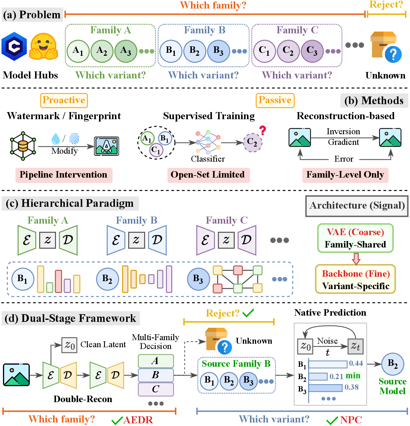
Denoising diffusion [1] and flow matching [2] have become the dominant paradigms in image generation, producing high-quality content from simple prompts [3]. As photorealism and semantic alignment continue to improve [4], generated imagery increasingly blurs the boundary between synthetic and authentic content, permeating creative design, film production, and other visual applications [5].
However, the democratization of image generation has also amplified misuse risks, as exemplified by fabricated Pentagon-explosion imagery [6]. Merely detecting whether an image is AI-generated is insufficient for accountability [7], [8]; reliable provenance requires tracing a suspect image back to the source model that produced it. This need is sharpened by the rapid expansion of open-weight generative ecosystems [9], [10]: public model hubs now host many checkpoints that are fine-tuned, distilled, or otherwise derived from a small set of shared base models (Fig. [1][(a)]). In such ecosystems, intellectual-property protection, license compliance, and responsibility attribution depend on identifying not merely the model family, but the exact within-family variant. Because these candidate models are themselves openly accessible, fine-grained attribution among highly similar within-family variants becomes a practically tractable yet still largely unsolved problem.
Existing attribution methods for generated images can be broadly divided into proactive and passive approaches (Fig. [1][(b)]). Proactive methods embed traceable signals, such as watermarks [11]–[18] or model fingerprints [19]–[22], during training or generation to establish ownership identifiers. However, they typically require intervening in model weights or generation pipelines, which may constrain deployment or compromise visual quality. Passive methods instead perform post-hoc attribution from image-intrinsic evidence, without prior intervention. Supervised passive methods [23]–[31] train on large-scale generated images, but often generalize poorly to non-candidate data and require retraining for new sources. More critically, the highly similar generative distributions of within-family variants make discriminative boundaries difficult to learn [27]. Reconstruction-based methods [32]–[34] instead exploit an intrinsic property: a source model exhibits stronger reconstruction or prediction consistency for images from its own distribution. This provides a training-free attribution signal compatible with open-set family-level scenarios, making such methods promising for real-world forensics.
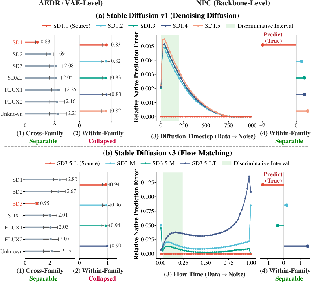
Within reconstruction-based attribution for latent generative models [3], LatentTracer [33] and AEDR [34] are two notable approaches. LatentTracer measures the reconstruction capability of candidate models through latent-space inversion and gradient-based optimization [35], using reconstruction error as the attribution signal. Our prior work, AEDR, replaces a single reconstruction error with a homogeneity-calibrated ratio of two cascaded variational autoencoder (VAE) reconstructions, yielding a more stable signal at substantially lower computational cost. However, AEDR derives its signal from VAE-level reconstruction behavior: when models within a family share identical or highly compatible VAEs, this signal cannot capture the subtle differences among within-family variants (see Fig. [2][, columns (1)–(2)]). This raises a central question: if VAE-level signals only reveal family-level membership, which component provides fine-grained model-level evidence?
This question prompts us to revisit the internal structure of latent generative models [3]. We observe an underexplored structural cue (Fig. [1][(c)]): attribution signals are naturally organized along the architectural hierarchy. Specifically, the VAE maps images between pixel and latent spaces [36], defining the latent distribution on which the generative backbone operates; the backbone in turn learns the denoising diffusion [1] or flow matching [2] process within this latent space. Because the two components are tightly coupled, within-family variants often share identical or highly compatible VAEs while their variant-specific differences mainly reside in the backbone. This hierarchy naturally separates attribution signals: VAE-level cues reveal family-level membership for coarse attribution, whereas backbone-level cues capture variant-specific behaviors for model-level attribution.
Building on this insight, we decouple the attribution task along the “VAE\(\rightarrow\)backbone” hierarchy into a “coarse\(\rightarrow\)fine” pipeline, aligning the attribution granularity with the signals carried by each architectural level. Specifically, we propose Dual-stage Native Attribution (DNA), a coarse-to-fine attribution framework comprising Autoencoder Double-Reconstruction (AEDR) [34] at the coarse-grained stage and Native Prediction Consistency (NPC) at the fine-grained stage (Fig. [1][(d)]). The former leverages family-shared VAE-level signals to rapidly narrow the search space from all candidate models to a family, while the latter exploits variant-specific backbone-level signals to distinguish within-family variants. Without additional neural-network training, DNA enables end-to-end attribution from family-level identification to exact source-model localization, combining efficient coarse-grained screening with precise fine-grained discrimination.
The coarse-grained stage builds on our prior work AEDR, using the homogeneity-calibrated VAE double-reconstruction ratio as a family-level signal to narrow the search space to a unique candidate family or reject unknown sources. The fine-grained stage introduces NPC, which exploits the native prediction consistency of the generative backbone: a source model is expected to produce lower and more stable prediction errors on perturbed latents derived from its belonging images (Fig. [2][, columns (3)–(4)]). NPC evaluates this consistency across multiple noise levels and maps the resulting errors into a normalized and calibrated score space. This formulation naturally accommodates both denoising diffusion and flow matching, enabling closed-set model-level attribution.
To support systematic evaluation of the proposed framework, we construct DNA-30K. It comprises 30,000 images from 24 candidate models across six model families, spanning both denoising diffusion and flow matching, together with images from non-candidate generators and natural-image datasets as unknown sources. Existing benchmarks [37]–[42] primarily focus on coarse-grained source identification across architectures or model families, with limited coverage of within-family variants and recently emerged flow-matching models. To the best of our knowledge, DNA-30K is the first benchmark to jointly support open-set family-level screening and closed-set within-family variant attribution.
Our key contributions are summarized as follows:
Hierarchical Attribution Insight. We reveal that attribution cues in latent generative models are stratified across architectural levels: the VAE mainly preserves family-level reconstruction signatures, while the backbone captures finer model-level prediction behaviors. Based on this, we propose a “coarse\(\rightarrow\)fine” decoupled paradigm along the “VAE\(\rightarrow\)backbone” hierarchy, formulating attribution as open-set family-level screening followed by closed-set within-family variant identification.
Unified Dual-Stage Framework. We propose DNA, comprising AEDR for open-set family-level screening and the newly introduced NPC for closed-set model-level attribution. NPC evaluates native prediction consistency across multiple noise levels under semantic guidance and produces normalized and calibrated scores, accommodating both denoising diffusion and flow matching.
Open-Set Benchmark. We construct DNA-30K, to our knowledge, the first benchmark to jointly support open-set family-level screening and closed-set within-family variant attribution. It comprises 30,000 images from 24 candidate models across six families spanning both denoising diffusion and flow matching, and further includes unknown sources (generated and natural images).
Systematic Evaluation. Extensive experiments on DNA-30K show that DNA achieves 89.11% end-to-end accuracy and outperforms the strongest baseline by 33.81%, even when AEDR is used as the coarse-grained family-screening stage for all baselines. DNA also remains stable with limited calibration samples, diverse sampling configurations, and candidate-set expansion.
Extension Statement. This work substantially extends our conference paper AEDR [34]. The conference version focused on VAE-level family attribution. This journal version advances from family-level to model-level attribution among within-family variants. While retaining AEDR as the coarse-grained stage and augmenting it with an open-set multi-family decision mechanism, we introduce the hierarchical attribution paradigm, the fine-grained NPC module, the DNA-30K open-set benchmark, and comprehensive evaluations.
2 Related Work↩︎
2.1 Latent Generative Models↩︎
Latent generative models have become a dominant approach for high-quality image synthesis [43] and can be categorized by their generative dynamics into two paradigms. Denoising diffusion models originate from DDPM [1] and were subsequently scaled to high-resolution synthesis by Latent Diffusion Models [3], which perform the diffusion process in a low-dimensional latent space defined by a pretrained VAE [36]. This design underlies the Stable Diffusion series [3], [44] and also supports Transformer-based diffusion architectures [45], which replace the U-Net backbone [46] for improved scalability. Flow matching models, represented by Flow Matching [2] and Rectified Flow [47], characterize generation through continuous probability paths and velocity-field modeling, and have become an important technical foundation for large-scale models such as Stable Diffusion 3 [48]. Both paradigms employ a pretrained VAE that defines the latent space for the backbone; Section 3 formalizes this unified view.
2.2 Proactive Attribution of Generated Images↩︎
Proactive attribution methods identify the source model by deliberately embedding traceable signals before, during, or after image generation, mainly including image watermarking and model fingerprinting. Image watermarking methods can be further divided into post-processing watermarks [11]–[14] and generative watermarks [15]–[18]. The former typically embed detectable signals in the pixel or frequency domain of generated images, and thus offer broad applicability. The latter integrate watermarking into the sampling process, latent representation, or decoder, aiming to achieve traceability while preserving generation quality. Representative methods include Stable Signature [18], Tree-Ring [17], and Gaussian Shading [15], which respectively introduce verifiable identifiers by fine-tuning the latent diffusion decoder, embedding structured watermark patterns into the initial diffusion noise, or mapping watermark information into latent representations.
Model fingerprinting methods [19]–[22], [49] assign source-specific signatures during data preparation, model training, or generation, enabling generated images to carry identifiable model-level traces. Artificial Fingerprints [19] is a representative work, embedding fingerprints into training data and exploiting their transferability to generative models. Later studies extend this idea to diffusion models by modulating model weights [21] or exploiting latent semantic dimensions as fingerprints [22]. Overall, proactive attribution can provide reliable provenance evidence when the generation pipeline is controllable, but it requires prior intervention and may introduce deployment constraints, additional overhead, or visual quality trade-offs. In contrast, passive attribution requires no pipeline modification and performs post-hoc source tracing from image-intrinsic features or model responses, making it more applicable to real-world scenarios.
2.3 Passive Attribution of Generated Images↩︎
One line of passive attribution methods relies on supervised learning [23]–[30], [50], [51], training discriminative models on images from multiple sources to capture source-specific statistical traces. Early studies showed that CNN-generated images often contain frequency artifacts induced by upsampling operations [23], indicating that generative models leave learnable traces in their outputs. Yu et al. further extended this idea from real/fake detection to multi-class source identification [25], advancing the development of generated-image attribution. In the diffusion era, De-Fake [26] trains classifiers on CLIP [52] features to identify images from multiple diffusion sources, while OCC-CLIP [50] formulates attribution as a few-shot one-class classification problem, learning prompt vectors to distinguish belonging from non-belonging images. Some recent works also explore open-set attribution [29], [30]. While these methods have demonstrated strong performance under supervised attribution settings, their reliance on coverage of training sources makes generalization to new sources and fine-grained within-family variants less straightforward.
Reconstruction-based methods form another line of passive attribution [32]–[34]. Rather than relying on additional training, these methods exploit an intrinsic property of generative models: a source model typically exhibits stronger reconstruction or prediction consistency for images from its own distribution. RONAN [32] is an early representative method, performing gradient-based inversion [53] from random initialization and using complexity-calibrated reconstruction errors as attribution signals. LatentTracer [33] transfers this idea to the latent space, conducting inversion over VAE-encoded latent variables to reduce attribution cost and improve applicability to latent generative models. Our prior work AEDR [34] replaces a single absolute reconstruction error with the ratio of two cascaded VAE reconstruction errors, and further calibrates this signal with image homogeneity to suppress content-complexity bias. This design improves the stability and discriminability of reconstruction-based attribution signals. Existing reconstruction-based methods typically exploit coarse signals from a single architectural level, making them more suitable for family-level screening than for discriminating highly similar within-family variants. Consequently, within-family variant attribution remains underexplored.
2.4 Benchmarks for Generative Image Attribution↩︎
| Benchmark | Models | Families | Denoise | Flow | Variants | Open-Set | Size |
|---|---|---|---|---|---|---|---|
| ForenSynths [24] | 6 | – | 72.4K | ||||
| Attribution88 [37] | 7 | – | 1.06M | ||||
| IFDL [38] | 10 | – | 1.9M | ||||
| OSMA [39] | 67 | – | 300K | ||||
| De-Fake [26] | 4 | – | 80K | ||||
| GenImage [40] | 8 | – | \(\bm{\triangle}\) | 2.68M | |||
| WildFake [41] | 21 | – | \(\bm{\triangle}\) | 3.57M | |||
| WILD [42] | 20 | – | \(\bm{\triangle}\) | 50K | |||
| DNA-30K | 24 | 6 | 30K |
2pt
With the development of generated image attribution, various forensic and attribution benchmarks have been constructed. Early benchmarks mainly focused on GAN-generated image detection and attribution, such as ForenSynths [24], GAN Fingerprints [25], and Attribution88 [37], which advanced this field from the perspectives of cross-generator generalization, model-fingerprint learning, and robust attribution representation. Later studies further extended benchmark construction to hierarchical image forensics, open-set model attribution, and synthetic-image association in real-world web scenarios, including IFDL [38], OSMA [39], and WILD [42]. Recent benchmarks such as GenImage [40] and WildFake [41] cover broader types of generative models, while WILD also includes DiT-based generators, providing important evaluation resources for source analysis across architectures.
As shown in Tab. 1, existing benchmarks have substantially advanced generated-image detection and attribution across architectures, model families, and real-world scenarios. However, they provide limited support for fine-grained attribution among highly similar within-family variants. Such variants often share backbone structures, training data, or latent representation spaces, making their differences much subtler than those across architectures or product-level models. This setting is therefore more challenging and closer to practical forensic demands. Meanwhile, public benchmarks for flow matching models such as Stable Diffusion 3 and FLUX, especially their within-family variants, remain limited. To fill this gap, we construct DNA-30K as a benchmark for within-family variant attribution under open-set family-level evaluation.
3 sec:Preliminaries↩︎
3.1 Variational Autoencoders↩︎
In mainstream latent generative models [3], [44], [48], [54], [55], the VAE [36] serves as a mapping component between pixel space and latent space, consisting of an encoder \(\mathcal{E}\) and a decoder \(\mathcal{D}\). The VAE is typically pretrained before the generative backbone and kept frozen during subsequent denoising diffusion or flow matching training, enabling generation in a low-dimensional latent space with significantly reduced computational cost. For notational simplicity, we absorb the scaling factor and its inverse into \(\mathcal{E}\) and \(\mathcal{D}\).
Given an image \(\mathbf{x}\), the VAE encoding and decoding are given by \(\mathbf{z}_0 = \mathcal{E}(\mathbf{x})\) and \(\tilde{\mathbf{x}} = \mathcal{D}(\mathbf{z}_0)\), where \(\mathbf{z}_0\) denotes the clean latent and \(\tilde{\mathbf{x}}\) the reconstructed image. We define the VAE reconstruction operator and reconstruction error as: \[\mathcal{R}(\mathbf{x}) \triangleq \mathcal{D}(\mathcal{E}(\mathbf{x})),\quad \ell_{\mathrm{rec}}(\mathbf{x}) = d_{\mathrm{rec}}\big(\mathbf{x},\, \mathcal{R}(\mathbf{x})\big), \label{VAE95Recon}\tag{1}\] where \(d_{\mathrm{rec}}(\cdot,\cdot)\) denotes a reconstruction distance such as pixel-level \(\ell_1\) or \(\ell_2\). For samples aligned with the VAE training distribution, \(\mathcal{R}\) approximates the identity mapping and thus yields small reconstruction errors. For samples deviating from this distribution, the VAE tends to project them toward the learned manifold, resulting in notable shifts. This asymmetric reconstruction behavior forms the basis of the family-level attribution signal in the coarse-grained stage (Sec. 5.1).
3.2 Denoising Diffusion Models↩︎
Denoising diffusion models [1] generate images by learning the reverse generative dynamics of perturbed latent representations across varying noise levels. For unified notation, we adopt the common \(\boldsymbol{\varepsilon}\)-prediction formulation. Given an image-condition pair \((\mathbf{x},\mathbf{c})\sim p_{\mathrm{data}}\), where \(p_{\mathrm{data}}\) denotes the data distribution and \(\mathbf{c}\) is the semantic condition, the clean latent is obtained as \(\mathbf{z}_0=\mathcal{E}(\mathbf{x})\). At a discrete timestep \(t\in\{1,\dots,T\}\), where \(T\) is the total number of diffusion steps, the forward process produces a perturbed latent \(\mathbf{z}_t = \sqrt{\bar{\alpha}_t}\,\mathbf{z}_0 + \sqrt{1-\bar{\alpha}_t}\,\boldsymbol{\varepsilon}\), where \(\boldsymbol{\varepsilon}\sim\mathcal{N}(\mathbf{0},\mathbf{I})\) denotes the injected standard Gaussian noise, and \(\bar{\alpha}_t=\prod_{s=1}^{t}(1-\beta_s)\) is the cumulative noise coefficient defined by the variance schedule \(\{\beta_t\}_{t=1}^{T}\).
The noise predictor \(\boldsymbol{\varepsilon}_{\theta}(\mathbf{z}_t,t,\mathbf{c})\), parameterized by the generative backbone parameters \(\theta\), is trained to estimate \(\boldsymbol{\varepsilon}\): \[\mathcal{L}_{\boldsymbol{\varepsilon}}(\theta) = \mathbb{E}\!\left[\left\|\boldsymbol{\varepsilon} - \boldsymbol{\varepsilon}_{\theta}(\mathbf{z}_t,t,\mathbf{c})\right\|_2^2\right], \label{DD95Loss}\tag{2}\] where the expectation is taken over \((\mathbf{x},\mathbf{c})\sim p_{\mathrm{data}}\), \(t\sim\mathcal{U}(\{1,\dots,T\})\), and \(\boldsymbol{\varepsilon}\sim\mathcal{N}(\mathbf{0},\mathbf{I})\). This objective defines the native prediction target of denoising diffusion backbones.
3.3 Flow Matching Models↩︎
Flow matching models learn a velocity field along a continuous probability path [2], [48], [54], [55]. For unified notation, we present the rectified flow formulation [47]. Given an image-condition pair \((\mathbf{x},\mathbf{c})\sim p_{\mathrm{data}}\), the clean latent is obtained as \(\mathbf{z}_0=\mathcal{E}(\mathbf{x})\). At continuous time \(t\in[0,1]\), the perturbed latent representation is \(\mathbf{z}_t = (1-t)\,\mathbf{z}_0 + t\,\boldsymbol{\varepsilon}\), \(\boldsymbol{\varepsilon}\sim\mathcal{N}(\mathbf{0},\mathbf{I})\), where \(t{=}0\) corresponds to the data endpoint and \(t{=}1\) to the noise endpoint. The corresponding target velocity is \(d\mathbf{z}_t/dt = \boldsymbol{\varepsilon}-\mathbf{z}_0\).
The velocity predictor \(\mathbf{v}_{\theta}(\mathbf{z}_t,t,\mathbf{c})\) with backbone parameters \(\theta\) is trained to estimate the target velocity \(\boldsymbol{\varepsilon}-\mathbf{z}_0\): \[\mathcal{L}_{\mathbf{v}}(\theta) = \mathbb{E}\!\left[\left\|(\boldsymbol{\varepsilon}-\mathbf{z}_0) - \mathbf{v}_{\theta}(\mathbf{z}_t,t,\mathbf{c})\right\|_2^2\right], \label{FM95Loss}\tag{3}\] where the expectation is over \((\mathbf{x},\mathbf{c})\sim p_{\mathrm{data}}\), \(t\sim\mathcal{U}([0,1])\), and \(\boldsymbol{\varepsilon}\sim\mathcal{N}(\mathbf{0},\mathbf{I})\). Although the path is defined from data to noise, sampling proceeds in reverse from noise to data.
3.4 Unified Native Prediction Objective↩︎
| Aspect | Denoising Diffusion | Flow Matching |
|---|---|---|
| Noise-level convention \(t\) | \(\{1,\dots,T\}\) | \([0,1]\) |
| Mixing coefficients \((a_t,b_t)\) | \((\sqrt{\bar{\alpha}_t},\sqrt{1-\bar{\alpha}_t})\) | \((1-t,t)\) |
| Native prediction target \(\mathbf{u}_t\) | \(\boldsymbol{\varepsilon}\) | \(\boldsymbol{\varepsilon}-\mathbf{z}_0\) |
| Backbone predictor \(\mathbf{f}_{\theta}\) | \(\boldsymbol{\varepsilon}_{\theta}(\mathbf{z}_t,t,\mathbf{c})\) | \(\mathbf{v}_{\theta}(\mathbf{z}_t,t,\mathbf{c})\) |
| Perturbed latent \(\mathbf{z}_t\) | \(a_t\mathbf{z}_0+b_t\boldsymbol{\varepsilon}\) | |
| Native prediction error | \(\|\mathbf{u}_t-\mathbf{f}_{\theta}(\mathbf{z}_t,t,\mathbf{c})\|_2^2\) | |
3pt
Despite different perturbation paths and prediction targets, denoising diffusion [4] and flow matching [2], [47] can be understood through a unified native prediction framework. As summarized in Tab. 2, both paradigms construct a perturbed latent \(\mathbf{z}_t = a_t\,\mathbf{z}_0 + b_t\,\boldsymbol{\varepsilon}\) with paradigm-specific mixing coefficients, and train the backbone predictor \(\mathbf{f}_{\theta}(\mathbf{z}_t,t,\mathbf{c})\) to estimate the corresponding native target \(\mathbf{u}_t\). Under this view, both paradigms share the unified training objective: \[\theta^{\star} = \arg\min_{\theta}\;\mathbb{E}\!\left[\left\|\mathbf{u}_t - \mathbf{f}_{\theta}(\mathbf{z}_t,t,\mathbf{c})\right\|_2^2\right], \label{DM95FM95Loss}\tag{4}\] where \(\theta^{\star}\) denotes the trained backbone parameters, and the expectation is taken over the training data, noise levels, and Gaussian noise under the corresponding paradigm.
This formulation shows that both types of generative backbones are optimized to minimize native prediction errors on perturbed latents from their own generative distributions. Thus, if an image originates from a specific source model, that model is expected to produce systematically lower prediction errors on the corresponding perturbed latents (see Fig. 2). This native prediction consistency motivates the model-level attribution signal used in the fine-grained stage (Sec. 5.2).
4 Problem Formulation↩︎
We aim to perform efficient and reliable source-model attribution of generated images from the perspective of an auditor without additional neural-network training; only a small calibration set is used to estimate family thresholds, discriminative timesteps, and scalar offsets. To facilitate the discussion, we first define belonging and non-belonging images, then introduce the model family structure, the attribution objective, and the corresponding access assumptions.
4.1 Belonging and Non-Belonging Images↩︎
Given an image generative model \(M\) and image space \(\mathcal{X}\), an image \(\mathbf{x}\in\mathcal{X}\) is called a belonging image of \(M\) if it is generated by \(M\), denoted by \(\mathrm{src}(\mathbf{x})=M\); otherwise it is a non-belonging image. Non-belonging images may originate from other known or unknown generative models, or from natural image distributions. This definition emphasizes the actual generative relationship between an image and its source model, rather than distributional overlap or visual similarity.
4.2 Model Families and Within-Family Variants↩︎
Existing latent generative models often exhibit pronounced familial relationships: a single base model or architecture gives rise to multiple variants through different training stages, fine-tuning strategies, or distillation configurations. These variants typically share the same VAE or highly compatible VAEs while differing in their generative backbones. Formally, given a candidate model set \(\mathcal{M}=\{M_1,\dots,M_N\}\), let \(V_i=(\mathcal{E}_i,\mathcal{D}_i)\) denote the VAE used by model \(M_i\). We partition \(\mathcal{M}\) into \(K\) disjoint model families based on VAE compatibility: \[\mathcal{M}=\bigcup_{k=1}^{K}\mathcal{F}_k, \quad \mathcal{F}_k=\{M_i\in\mathcal{M}\mid V_i \simeq V^{(k)}\}, \label{eq:family}\tag{5}\] where \(V^{(k)}\) is the representative VAE of model family \(\mathcal{F}_k\), and \(V_i \simeq V^{(k)}\) indicates that \(M_i\) uses the same or highly compatible VAE, i.e., both encode to and decode from the shared latent space with negligible distributional mismatch. Models \(M_i, M_j \in \mathcal{F}_k\) are called within-family variants.
4.3 Attribution Objective↩︎
Given the candidate model set \(\mathcal{M}\) and its family partition \(\{\mathcal{F}_k\}_{k=1}^{K}\), the goal is to attribute a query image \(\mathbf{x}\) to its source model. If \(\mathrm{src}(\mathbf{x})\in\mathcal{M}\), the auditor should identify its exact source model; otherwise, if \(\mathrm{src}(\mathbf{x})\notin\mathcal{M}\), the image should be rejected as coming from an unknown source. We decompose this attribution objective into two stages.
Stage 1: Coarse-grained family-level attribution. The first stage performs open-set family attribution [56], [57], determining whether \(\mathbf{x}\) can be assigned to a known model family. Let \(\Phi_{\mathrm{coarse}}\) denote the coarse attribution function, with output \(\hat{\mathcal{F}}=\Phi_{\mathrm{coarse}}(\mathbf{x}) \in \{\mathcal{F}_1,\dots,\mathcal{F}_K\}\cup\{\varnothing\}\), where \(\hat{\mathcal{F}}\) is the predicted model family and \(\varnothing\) indicates an open-set rejection label, meaning that no unique candidate-family assignment is made. If \(\hat{\mathcal{F}}=\varnothing\), the attribution process terminates and no fine-grained model decision is performed.
Stage 2: Fine-grained model-level attribution. When \(\hat{\mathcal{F}}\neq\varnothing\), the second stage performs closed-set model attribution within the predicted family \(\hat{\mathcal{F}}\). Let \(\Phi_{\mathrm{fine}}\) denote the fine-grained attribution function. It outputs \(\hat{M}=\Phi_{\mathrm{fine}}(\mathbf{x};\hat{\mathcal{F}})\), where \(\hat{M}\in\hat{\mathcal{F}}\). Since this stage is restricted to the family selected by Stage 1, the candidate space is reduced from all models to a compact set of within-family variants.
We emphasize that open-set handling is confined to Stage 1, which is designed to reject inputs outside the candidate family set. Conditional on acceptance into a candidate family, Stage 2 operates in a closed-set setting and assumes that the within-family candidate variants are known. This setting is aligned with open-weight model auditing, in which the relevant public or versioned checkpoints can be enumerated. Rejecting an unknown within-family variant constitutes a more challenging open-set problem and falls outside the primary scope of DNA; nevertheless, we provide a preliminary leave-one-out analysis in Sec. 8 to assess its feasibility and challenges.
End-to-end correctness. Let \(\mathcal{F}^{\star}\) denote the true source family of \(\mathbf{x}\): \(\mathcal{F}^{\star}=\mathcal{F}_k\) if \(\mathrm{src}(\mathbf{x})\in\mathcal{F}_k\), and \(\mathcal{F}^{\star}=\varnothing\) if \(\mathrm{src}(\mathbf{x})\notin\mathcal{M}\). We define the end-to-end correctness predicate \(\mathrm{E2E}(\mathbf{x})\), which holds if and only if: \[\mathrm{E2E}(\mathbf{x}) \Longleftrightarrow \begin{cases} \hat{\mathcal{F}}=\mathcal{F}^{\star} \;\text{and}\; \hat{M}=\mathrm{src}(\mathbf{x}), & \text{if } \mathcal{F}^{\star}\neq\varnothing,\\[4pt] \hat{\mathcal{F}}=\varnothing, & \text{if } \mathcal{F}^{\star}=\varnothing. \end{cases} \label{eq:e2e}\tag{6}\]
This criterion requires correct open-set rejection for unknown sources and, for known source images, correct family identification and source-model attribution, thereby reflecting the precision demanded in real-world forensic scenarios.
4.4 Access Assumptions↩︎
As motivated in Sec. 1, DNA targets open-weight auditing scenarios in which the candidate model checkpoints are publicly available to the auditor. We formalize this operating premise by specifying the access assumptions for each stage.
Stage 1: VAE-only access. In this stage, we assume that the auditor can access only the VAE of each candidate family, without accessing the corresponding generative backbones. This VAE-only assumption is less demanding than approaches requiring full white-box access [32], [33] to the entire model. It also aligns with the family structure defined in Sec. 4.2: since within-family variants often share the same VAE or highly compatible VAEs, maintaining one representative VAE per family is sufficient for family-level screening, reducing the maintenance cost when new families are added.
Stage 2: Forward-only backbone access. In this stage, we assume that the auditor has forward-only access to the generative backbones of the variants within the predicted family \(\hat{\mathcal{F}}\). The auditor can query each backbone \(\mathbf{f}_{\theta}(\mathbf{z}_t,t,\mathbf{c})\) with a perturbed latent \(\mathbf{z}_t\), a noise level \(t\), and a condition \(\mathbf{c}\), and obtain only its native prediction output; no gradient access or parameter updates are required. The query burden of this assumption is controlled by the problem structure and practical auditing scenarios. (i) Stage 1 has already narrowed the search space from the entire candidate pool to a single family, so forward access is required only for the small set of within-family variants. (ii) Within-family variants often share the same development lineage and are released as related checkpoints or derived from public base weights, making family-level auditing a natural operational unit.
Together, the two-stage access assumptions align with the attribution granularity: the coarse stage performs open-set family-level attribution with minimal VAE-level access, while the fine stage performs precise discrimination within a compact within-family candidate set using forward-only backbone queries. This formulation establishes the deployment setting for the method introduced in Sec. 5.
5 Methodology↩︎
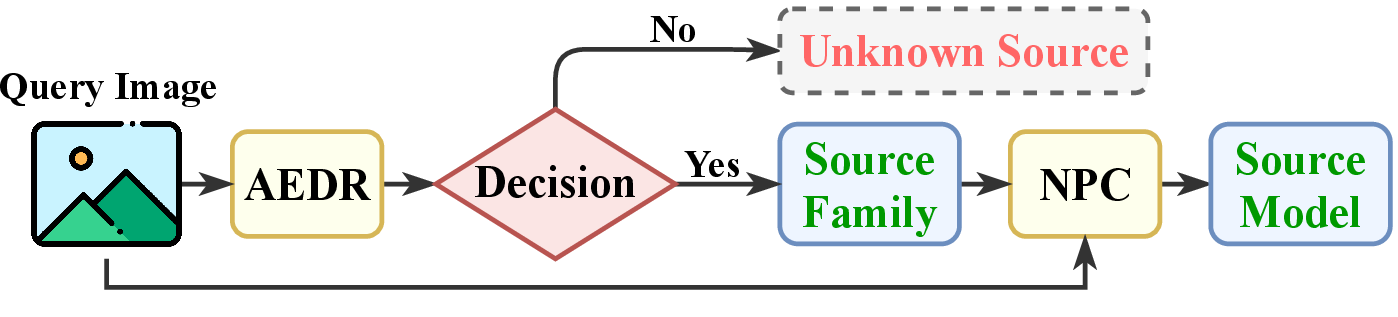
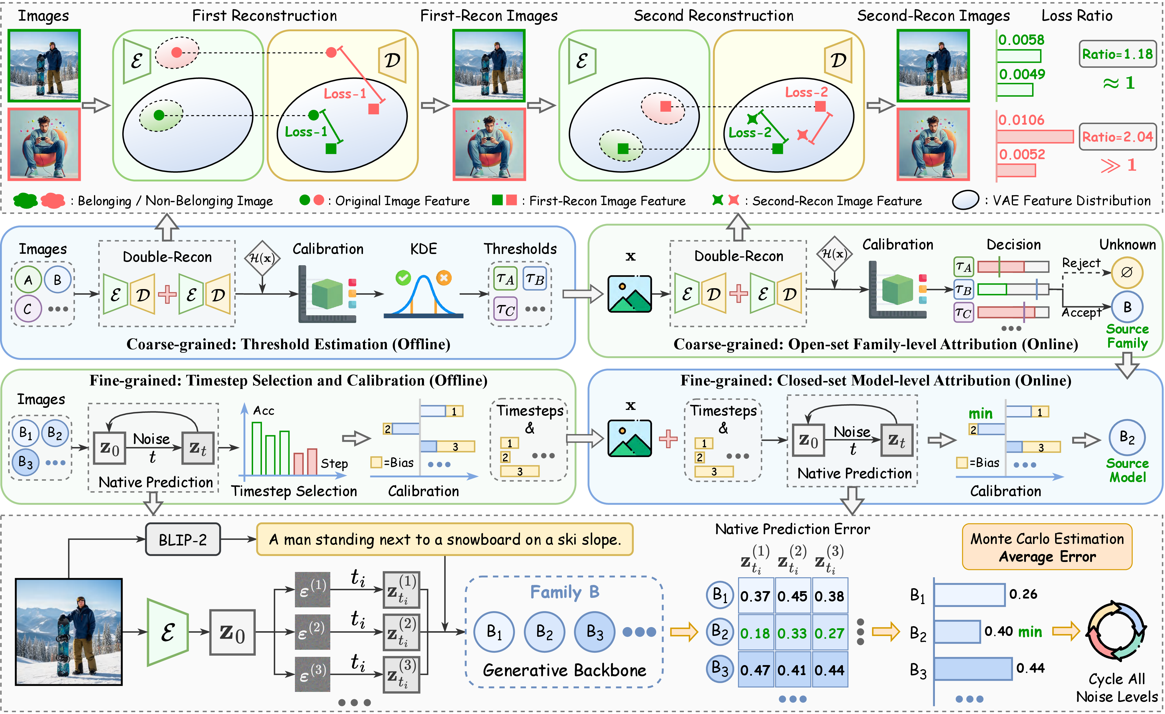
DNA follows the two-stage attribution framework defined in Sec. 4, leveraging complementary attribution signals at the VAE and backbone levels of latent generative models. The coarse-grained stage builds on our prior work AEDR [34] and extends it with a multi-family open-set decision mechanism. The fine-grained stage introduces NPC for closed-set model-level attribution, which operates under the unified native prediction objective (Sec. 3.4) to support both \(\boldsymbol{\varepsilon}\)-prediction and \(\mathbf{v}\)-prediction paradigms. As illustrated in Figs. 3 and 4, DNA performs open-set family-level attribution (Stage 1, AEDR) to narrow the candidate space to a single family, then closed-set model-level attribution (Stage 2, NPC) to identify the source variant within that family. In DNA, training-free means that no gradient-based parameter updates are applied to any VAE or generative backbone, and no auxiliary attribution network is trained; a small labeled calibration set is used only for non-gradient-based threshold estimation, discriminative-timestep selection, and consistency score calibration.
5.1 Coarse-Grained Stage: AEDR (Stage 1)↩︎
5.1.1 VAE Double-Reconstruction Signal↩︎
Building on the asymmetric reconstruction behavior described in Sec. 3.1, AEDR exploits the observation that a VAE responds differently to belonging and non-belonging images across two reconstructions. Given the VAE reconstruction operator \(\mathcal{R}_k\) of candidate family \(\mathcal{F}_k\) and a query image \(\mathbf{x}\), we perform two cascaded reconstructions and record the corresponding losses: \[\mathbf{x}_k^{(1)}=\mathcal{R}_k(\mathbf{x}), \qquad \ell_k^{(1)}(\mathbf{x})=d_{\mathrm{mse}}\!\left(\mathbf{x}_k^{(1)},\,\mathbf{x}\right), \label{eq:recon1}\tag{7}\] \[\mathbf{x}_k^{(2)}=\mathcal{R}_k\!\left(\mathbf{x}_k^{(1)}\right), \qquad \ell_k^{(2)}(\mathbf{x})=d_{\mathrm{mse}}\!\left(\mathbf{x}_k^{(2)},\,\mathbf{x}_k^{(1)}\right), \label{eq:recon2}\tag{8}\] where \(d_{\mathrm{mse}}(\cdot,\cdot)\) denotes the mean squared error (MSE), and \(\mathbf{x}_k^{(1)}\), \(\mathbf{x}_k^{(2)}\) are the first and second reconstructed images.
The key intuition is as follows. For a belonging image \(\mathrm{src}(\mathbf{x})\in\mathcal{F}_k\), the image already lies near the VAE training manifold, so both reconstructions produce similar losses, i.e., \(\ell_k^{(2)}(\mathbf{x})\approx\ell_k^{(1)}(\mathbf{x})\). For a non-belonging image \(\mathrm{src}(\mathbf{x})\notin\mathcal{F}_k\), the first reconstruction projects it from an out-of-distribution region toward the VAE manifold with a higher loss, while the second operates on the already-projected \(\mathbf{x}_k^{(1)}\) and yields a much smaller loss, i.e., \(\ell_k^{(2)}(\mathbf{x})\ll\ell_k^{(1)}(\mathbf{x})\). Based on this asymmetric behavior, we define the VAE-level family attribution signal as the ratio between the two losses: \[r_k(\mathbf{x})=\frac{\ell_k^{(1)}(\mathbf{x})}{\ell_k^{(2)}(\mathbf{x})}. \label{eq:ratio}\tag{9}\] For belonging images, \(r_k(\mathbf{x})\approx 1\), while for non-belonging images \(r_k(\mathbf{x})\gg 1\), providing a more stable family-level signal than a single absolute reconstruction error [32]–[34].
5.1.2 Homogeneity Calibration↩︎
Although the double-reconstruction ratio \(r_k(\mathbf{x})\) is more stable than a single absolute reconstruction error [34], its fluctuations can still be affected by the intrinsic content complexity of the image. To mitigate this bias, we introduce a homogeneity calibration based on the gray-level co-occurrence matrix (GLCM): \[\mathcal{H}(\mathbf{x}) = \sum_{i=0}^{Q-1}\sum_{j=0}^{Q-1}\frac{P_{\mathbf{x}}(i,j)}{1+|i-j|}, \;\; \tilde{r}_k(\mathbf{x}) = \mathcal{H}(\mathbf{x})\cdot r_k(\mathbf{x}), \label{eq:calibration}\tag{10}\] where \(P_{\mathbf{x}}(i,j)\) denotes the normalized co-occurrence probability of gray levels \(i\) and \(j\) in image \(\mathbf{x}\) under a predefined direction and offset, and \(Q\) is the number of gray-level quantization bins, set to \(32\) by default. A larger \(\mathcal{H}(\mathbf{x})\) indicates smoother local gray-level variations and stronger content homogeneity, whereas a smaller value suggests more complex texture structures. The calibrated signal \(\tilde{r}_k(\mathbf{x})\) is then used for subsequent family-level attribution decisions.
5.1.3 Threshold Determination via KDE↩︎
The calibrated signal \(\tilde{r}_k(\mathbf{x})\) exhibits different non-parametric distributions across model families, making a single global threshold unsuitable. Therefore, we independently estimate a family-specific adaptive threshold from the signal distribution of belonging images. Given \(n\) belonging calibration images from family \(\mathcal{F}_k\), with calibrated signals \(\{\tilde{r}_{k,i}\}_{i=1}^{n}\) (default \(n{=}100\)), we estimate the empirical density using kernel density estimation (KDE) [58] and set the family threshold as the \((1-\alpha)\) quantile: \[\tau_k = \inf\!\Bigg\{\:u \,\Big|\: \int_{-\infty}^{u} \frac{1}{nh}\sum_{i=1}^{n}\mathcal{K}\:\left(\frac{y-\tilde{r}_{k,i}}{h}\right)dy \:\ge\: 1-\alpha\,\Bigg\}. \label{eq:kde}\tag{11}\] Here, \(\mathcal{K}(\cdot)\) is a Gaussian kernel, \(h\) is the kernel bandwidth, and \(\alpha\) is a tail tolerance parameter (default \(\alpha{=}0.03\)) controlling the threshold sensitivity to extreme samples. An image \(\mathbf{x}\) is classified as belonging to family \(\mathcal{F}_k\) if \(\tilde{r}_k(\mathbf{x})\leq\tau_k\), and as non-belonging otherwise. Since KDE makes no parametric assumptions, the resulting threshold \(\tau_k\) adapts naturally to the calibrated signal distribution of each family.
5.1.4 Multi-Family Open-Set Decision↩︎
We instantiate the coarse attribution function \(\Phi_{\mathrm{coarse}}\) defined in Sec. 4.3 using AEDR [34]. A straightforward solution would be to formulate it as an open-set multi-class classifier, but this is not well aligned with the nature of AEDR signals. For each family \(\mathcal{F}_k\), the calibrated signal \(\tilde{r}_k(\mathbf{x})\) only measures whether \(\mathbf{x}\) conforms to the VAE reconstruction behavior of that family, and the threshold \(\tau_k\) defines a family-specific acceptance boundary. Therefore, \(\tilde{r}_k(\mathbf{x})\) should be treated as an intrinsic family-wise decision statistic rather than a globally comparable score across families. Accordingly, we adopt \(K\) parallel family-wise threshold tests. Let \(\mathcal{A}(\mathbf{x})=\{\mathcal{F}_k \mid \tilde{r}_k(\mathbf{x})\leq\tau_k,\;k=1,\dots,K\}\) denote the set of families that accept \(\mathbf{x}\). The coarse-grained output follows a unique-acceptance rule: \[\hat{\mathcal{F}} = \Phi_{\mathrm{coarse}}(\mathbf{x}) = \begin{cases} \mathcal{F}_k, & \text{if } \mathcal{A}(\mathbf{x})=\{\mathcal{F}_k\},\\[4pt] \varnothing, & \text{if } |\mathcal{A}(\mathbf{x})|\neq 1. \end{cases} \label{eq:coarse-decision}\tag{12}\]
Under this rule, AEDR proceeds to the fine-grained stage only when exactly one candidate family accepts \(\mathbf{x}\). If no family accepts \(\mathbf{x}\), or if multiple families accept it simultaneously, the coarse stage outputs the open-set rejection label \(\varnothing\), indicating that no unique and reliable known family can be assigned. This parallel thresholding rule matches the family-intrinsic nature of AEDR signals and scales naturally. When a new family \(\mathcal{F}_{K+1}\) is introduced, only its calibrated signal distribution and decision threshold need to be estimated, without recalibrating or modifying the existing family-wise decision rules.
5.2 Fine-Grained Stage: NPC (Stage 2)↩︎
Once exactly one candidate family is identified, Stage 1 restricts the candidate set to the variants within that family. Since within-family variants share the same VAE, VAE-level signals are insufficient for further discrimination. To achieve closed-set model-level attribution, we propose NPC, which directly compares the native prediction errors of within-family candidate backbones under shared semantic conditioning and identical perturbed latent inputs. As discussed in Sec. 3, the source backbone is expected to exhibit stronger native prediction consistency—and thus lower prediction errors—than non-source candidates (see Fig. [2][, columns (3)–(4)]).
5.2.1 Semantically Conditioned Native Prediction↩︎
Let \(\hat{\mathcal{F}}=\Phi_{\mathrm{coarse}}(\mathbf{x})\) be the predicted family from AEDR [34]. When \(\hat{\mathcal{F}}=\mathcal{F}_{\hat{k}}\neq\varnothing\), we re-index the within-family variants as \(\mathcal{F}_{\hat{k}}=\{M_1,\dots,M_J\}\) for notational simplicity, where \(J=|\mathcal{F}_{\hat{k}}|\) is the number of within-family variants. NPC first extracts a semantic condition \(\mathbf{c}\) from the query image \(\mathbf{x}\) using BLIP-2 [59]. This condition is shared by all candidate backbones, so that the comparison of prediction errors is less affected by semantic discrepancies and more directly reflects how well each generative backbone fits the query image \(\mathbf{x}\).
The image \(\mathbf{x}\) is encoded into a clean latent \(\mathbf{z}_0=\mathcal{E}_{\hat{k}}(\mathbf{x})\) via the family-shared VAE encoder. Given a candidate timestep set \(\mathcal{T}_{\hat{k}}=\{t_1,\dots,t_L\}\), NPC samples \(S\) independent Gaussian noise vectors \(\{\boldsymbol{\varepsilon}^{(s)}\}_{s=1}^{S}\!\overset{\mathrm{i.i.d.}}\sim\!\mathcal{N}(\mathbf{0},\mathbf{I})\) at each timestep \(t_i\). To ensure fair comparison, the same noise samples are shared across all candidate variants at each timestep. Following the unified formulation in Tab. 2, the perturbed latent is \(\mathbf{z}_{t_i}^{(s)}=a_{t_i}\mathbf{z}_0+b_{t_i}\boldsymbol{\varepsilon}^{(s)}\) and the native prediction target is \(\mathbf{u}_{t_i}^{(s)}\), instantiated as \(\boldsymbol{\varepsilon}^{(s)}\) for denoising diffusion and \(\boldsymbol{\varepsilon}^{(s)}-\mathbf{z}_0\) for flow matching. The native prediction error of candidate variant \(M_j\) at timestep \(t_i\) with noise sample \(s\) is: \[e_{j,t_i}^{(s)} = \left\|\mathbf{u}_{t_i}^{(s)} - \mathbf{f}_{\theta_j}\!\left(\mathbf{z}_{t_i}^{(s)},\,t_i,\,\mathbf{c}\right)\right\|_2^2, \label{eq:npc-error}\tag{13}\] where \(\mathbf{f}_{\theta_j}\) is the backbone predictor of \(M_j\), corresponding to \(\boldsymbol{\varepsilon}_{\theta_j}\) for denoising diffusion or \(\mathbf{v}_{\theta_j}\) for flow matching. Since the true expectation over \(\boldsymbol{\varepsilon}\) generally has no closed-form expression, NPC approximates it via Monte Carlo [60] estimation with \(S\) independent noise samples, reducing the variance introduced by any single random perturbation: \[\mu_{j,t_i} \!=\! \frac{1}{S}\sum_{s=1}^{S}e_{j,t_i}^{(s)} \!\xrightarrow{\,S\to\infty\,}\! \mathbb{E}_{\boldsymbol{\varepsilon}}\!\left[\left\|\mathbf{u}_{t_i} \!- \mathbf{f}_{\theta_j}(\mathbf{z}_{t_i},\,t_i,\,\mathbf{c})\right\|_2^2\right]. \label{eq:npc-mu}\tag{14}\] The quantity \(\mu_{j,t_i}\) characterizes the native prediction consistency of candidate variant \(M_j\) at noise level \(t_i\) under the given semantic condition. If \(\mathbf{x}\) originates from \(M_j\), the corresponding perturbed latents are expected to be better aligned with the generative distribution of \(M_j\), leading to systematically lower native prediction errors. This relative difference across within-family variants serves as the basis for the subsequent timestep selection, score normalization, and final decision.
5.2.2 Discriminative Timestep Selection↩︎
Despite their architectural similarity, within-family variants exhibit different degrees of separability in native prediction error across noise levels: some timesteps clearly distinguish the source from non-source candidates, whereas others are considerably less discriminative (see Fig. [2][, columns (3)–(4)]). Indiscriminately aggregating all timesteps may therefore dilute the discriminative signal from the most informative ones. Accordingly, NPC uses a small labeled calibration set to select a family-specific subset of discriminative timesteps \(\mathcal{T}_{\hat{k}}^{\star}\subseteq\mathcal{T}_{\hat{k}}\).
Specifically, let \(\{(\mathbf{x}_i,j_i^{\star})\}_{i=1}^{n_{\mathrm{cal}}}\) be the calibration set from family \(\mathcal{F}_{\hat{k}}\), comprising \(n\) labeled images per variant, i.e., \(n_{\mathrm{cal}}=n\times{J}\) with \(n=100\) by default. Here, \(j_i^{\star}\in\{1,\dots,J\}\) denotes the ground-truth source-model index of \(\mathbf{x}_i\). For each candidate timestep \(t\in\mathcal{T}_{\hat{k}}\), we define its single-timestep attribution accuracy \(p_{\hat{k}}(t)\) as the fraction of calibration samples correctly attributed when the decision is made solely based on the native prediction errors \(\mu_{j,t}(\mathbf{x}_i)\) at that timestep: \[p_{\hat{k}}(t) = \frac{1}{n_{\mathrm{cal}}}\sum_{i=1}^{n_{\mathrm{cal}}}\mathbb{1}\!\left[\arg\min_{j\in\{1,\dots,J\}}\mu_{j,t}(\mathbf{x}_i)=j_i^{\star}\right]. \label{eq:timestep-acc}\tag{15}\]
The discriminative timestep set is then obtained by selecting the top-\(L^{\star}\) timesteps with the highest \(p_{\hat{k}}(t)\): \(\mathcal{T}_{\hat{k}}^{\star}=\mathrm{Top}_{L^{\star}}(\mathcal{T}_{\hat{k}};\,p_{\hat{k}}(t))\), where \(L^{\star}\leq L=|\mathcal{T}_{\hat{k}}|\). The selection is performed independently for each model family, thereby retaining the timesteps that are most informative for discriminating among its within-family variants. Empirically, timesteps closer to the noise endpoint tend to make perturbed latents approach pure Gaussian noise, substantially weakening latent-space structure and increasingly obscuring variant-specific prediction differences with random perturbations. In contrast, low-to-intermediate noise levels better preserve latent structure (see Fig. [2][, column (3)]), enabling NPC to reveal subtle differences among within-family variants under shared semantic conditioning. The data-driven selection therefore tends to favor these more informative and discriminative timesteps.
5.2.3 Normalized and Calibrated Consistency Scores↩︎
Raw native prediction errors are insufficient for high-precision attribution. First, error magnitudes vary substantially across timesteps, allowing timesteps with larger error scales to dominate the aggregation and obscure discriminative relative differences. Second, within-family variants may exhibit variant-specific error offsets due to differences in training strategies, potentially masking the expected minimum-error advantage of the source model. To address these issues, NPC constructs consistency scores through normalization and calibration.
Cross-model z-score normalization. At each selected timestep \(t_i\in\mathcal{T}_{\hat{k}}^{\star}\), we normalize the native prediction errors across the \(J\) within-family variants: \[\tilde{\mu}_{j,t_i} = \frac{\mu_{j,t_i}-\bar{\mu}_{\cdot,t_i}}{\sigma_{\cdot,t_i}}, \quad \bar{\mu}_{\cdot,t_i}=\frac{1}{J}\sum_{j=1}^{J}\mu_{j,t_i}, \label{eq:zscore}\tag{16}\] where \(\sigma_{\cdot,t_i}\) is the standard deviation across variants at timestep \(t_i\). This normalization aligns errors from different timesteps to a common scale and exposes variant-specific biases as separable constant offsets. Averaging over the discriminative timestep set yields the base consistency score: \[s_j(\mathbf{x}) = \frac{1}{L^{\star}}\sum_{t_i\in\mathcal{T}_{\hat{k}}^{\star}}\tilde{\mu}_{j,t_i}. \label{eq:base-score}\tag{17}\]
Model-level calibration. To compensate for the constant offsets exposed by normalization, we introduce a family-specific scalar calibration term \(b_j^{(\hat{k})}\) for each candidate variant, yielding the final calibrated consistency score: \[S_j(\mathbf{x}) = s_j(\mathbf{x}) + b_j^{(\hat{k})}. \label{eq:calibrated-score}\tag{18}\] This calibration does not update any generative backbone or train an additional attribution classifier; it estimates only one scalar offset for each candidate variant within a family.
To avoid redundancy, we fix \(b_1^{(\hat{k})}=0\) for a reference model and estimate the remaining \(J{-}1\) scalars by maximizing the discrete, non-differentiable accuracy on the calibration set. Because the resulting parameter space is low-dimensional, we adopt a coarse-to-fine adaptive search [61], with an initial search interval derived from the range of base-score differences \(\{s_j(\mathbf{x}_i)-s_1(\mathbf{x}_i)\}\) observed on the calibration set. The search is then iteratively refined around the current best solution. This procedure introduces negligible overhead while effectively compensating for residual variant-specific biases.
5.2.4 Within-Family Closed-Set Attribution↩︎
Combining the preceding components, NPC performs fine-grained closed-set attribution by selecting the within-family variant with the minimum calibrated consistency score: \[\hat{M} = \arg\min_{M_j\in\mathcal{F}_{\hat{k}}} S_j(\mathbf{x}) = \arg\min_{M_j\in\mathcal{F}_{\hat{k}}}\left[s_j(\mathbf{x}) + b_j^{(\hat{k})}\right]. \label{eq:npc-decision}\tag{19}\] By aggregating native prediction errors over the selected discriminative timesteps and applying cross-model normalization and model-level calibration, NPC produces comparable consistency scores that highlight subtle variant-specific differences, enabling reliable within-family source attribution.
5.3 End-to-End Inference Pipeline↩︎
Following the two-stage formulation in Sec. 4.3, the end-to-end execution of DNA serially combines AEDR and NPC. Given a query image \(\mathbf{x}\), DNA first invokes \(K\) parallel family-wise threshold tests for open-set family screening, producing a candidate family \(\hat{\mathcal{F}}\). If \(\hat{\mathcal{F}}=\varnothing\) (unknown or ambiguous source), the system terminates with an open-set rejection. If \(\hat{\mathcal{F}}=\mathcal{F}_{\hat{k}}\), DNA proceeds to invoke NPC within that family for model-level attribution. The end-to-end decision is: \[\Phi_{\mathrm{DNA}}(\mathbf{x}) = \begin{cases} \Phi_{\mathrm{fine}}(\mathbf{x};\,\mathcal{F}_{\hat{k}}), & \text{if } \Phi_{\mathrm{coarse}}(\mathbf{x})=\mathcal{F}_{\hat{k}},\\[4pt] \varnothing, & \text{if } \Phi_{\mathrm{coarse}}(\mathbf{x})=\varnothing, \end{cases} \label{eq:dna-decision}\tag{20}\] where \(\Phi_{\mathrm{coarse}}\) is instantiated by AEDR (Eq. 12 ) and \(\Phi_{\mathrm{fine}}\) by NPC (Eq. 19 ). This serial structure strictly aligns with the end-to-end correctness criterion in Eq. 6 : an attribution is correct only when AEDR identifies the true source family \(\hat{\mathcal{F}}=\mathcal{F}^{\star}\) and NPC identifies the true source model \(\hat{M}=\mathrm{src}(\mathbf{x})\).
6 Benchmark: DNA-30K↩︎
| Family | Model / Dataset | Resolution | Steps | GS |
|---|---|---|---|---|
| SD1.x | Stable-Diffusion-v1-1 | 512\(\times\)512 | 50 | 7.5 |
| Stable-Diffusion-v1-2 | ||||
| Stable-Diffusion-v1-3 | ||||
| Stable-Diffusion-v1-4 | ||||
| Stable-Diffusion-v1-5 | ||||
| SD2.x | Stable-Diffusion-2-base | 512\(\times\)512 | 50 | 7.5 |
| Stable-Diffusion-2-1-base | ||||
| Stable-Diffusion-2-typography | ||||
| Stable-Diffusion-2-cartoon-blip | ||||
| SD3.x | Stable-Diffusion-3-medium | 1024\(\times\)1024 | 28 | 7.0 |
| Stable-Diffusion-3.5-medium | 40 | 4.5 | ||
| Stable-Diffusion-3.5-large | 28 | 3.5 | ||
| Stable-Diffusion-3.5-large-turbo | 4 | 0 | ||
| SDXL | Stable-Diffusion-xl-base-0.9 | 1024\(\times\)1024 | 40 | 7.5 |
| Stable-Diffusion-xl-base-1.0 | 40 | 7.5 | ||
| SSD-1B | 30 | 7.5 | ||
| Segmind-Vega | 25 | 9.0 | ||
| FLUX.1 | FLUX.1-dev | 1024\(\times\)1024 | 50 | 3.5 |
| FLUX.1-Krea-dev | 28 | 3.5 | ||
| FLUX.1-lite-8B | 28 | 3.5 | ||
| Chroma1-HD | 40 | 3.0 | ||
| FLUX.2 | FLUX.2-dev | 1024\(\times\)1024 | 50 | 4.0 |
| FLUX.2-klein-base-4B | ||||
| FLUX.2-klein-base-9B | ||||
| Unknown | PixArt-XL-2-1024-MS | 1024\(\times\)1024 | 20 | 4.5 |
| Qwen-Image | 1024\(\times\)1024 | 50 | 3.0 | |
| Kandinsky-3 | 1024\(\times\)1024 | 25 | 3.0 | |
| MS COCO (Real) | 287-640\(\times\)270-640 | – | – | |
| LAION (Real) | 287-640\(\times\)270-640 | – | – | |
| ImageNet (Real) | 512\(\times\)512 | – | – |
2.5pt
To support systematic evaluation of fine-grained within-family attribution, we construct DNA-30K—to our knowledge, the first benchmark to jointly evaluate family-level open-set screening and closed-set attribution among within-family variants of latent generative models. It comprises 24 candidate models from six model families, spanning both denoising diffusion and flow matching. For open-set family-level evaluation, DNA-30K additionally includes 3,000 images generated by three non-candidate models and 3,000 natural images drawn equally from MS COCO [62], ImageNet [63], and LAION [64] as unknown sources. Detailed compositions, resolutions, and sampling configurations are reported in Tab. 3.
The data generation protocol is designed to minimize evaluation bias. All generated images are conditioned on human-annotated MS COCO captions [65]. Within each split, the same caption set is used across models to control semantic variation, while the calibration and test caption sets are mutually disjoint. Each source contributes 1,000 images, evenly divided into a 500-image calibration split and a 500-image test split. The two splits are disjoint in image identity for all sources and in caption identity for all generated sources. The calibration split is used exclusively for threshold estimation, discriminative-timestep selection, and scalar score calibration; all reported results are computed on the held-out test split.
Except for the configuration-matched families described below, each candidate model uses its officially recommended default sampling configuration, reflecting how publicly released models are typically used in practice [9], [10]. In total, DNA-30K contains 27,000 generated images and 3,000 natural images, yielding 30,000 images. The benchmark will be publicly released to facilitate future research.
To reduce potential confounding from generation settings, we additionally match the scheduler, number of sampling steps, guidance scale, and resolution across all within-family variants in SD1.x, SD2.x, and FLUX.2 (see Tab. 3). This controlled setting limits the influence of the matched sampling factors on attribution performance and provides a stricter evaluation of whether NPC captures variant-specific backbone behavior rather than generation-configuration shortcuts.
7 Experiments↩︎
7.1 Experimental Setup↩︎
7.1.1 Models and data↩︎
All methods strictly follow the calibration/test split defined in DNA-30K. The calibration set is used only for threshold estimation, discriminative-timestep selection, and scalar score calibration in DNA, and for training or adaptation when required by the baselines, whereas the test set is reserved exclusively for independent evaluation.
7.1.2 Baselines↩︎
We select representative baselines from three technical categories: (1) CLIP-based few-shot attribution—OCC-CLIP [50], which learns prompt vectors with a frozen CLIP encoder to distinguish belonging from non-belonging images; (2) supervised discriminative attribution—De-Fake-Image (Img) and De-Fake-Hybrid (Hyb) [26], where the former trains a classifier using image features alone, whereas the latter additionally incorporates CLIP-derived visual and semantic features [52]; and (3) reconstruction-based attribution—LatentTracer [33], which measures the reconstruction capability of candidate models through latent-space inversion and gradient-based optimization [35].
For a fair comparison, we use the official open-source implementations and recommended hyperparameters for all baselines. OCC-CLIP [50] and LatentTracer [33] follow their default protocols, using 50 and 500 images per model, respectively, whereas De-Fake [26] uses the full 500-image budget per model available in DNA-30K. Since existing methods do not directly target within-family variant attribution, we adapt each baseline to our two-stage protocol: Stage 1 performs parallel family-wise binary tests, and Stage 2 conducts \(J\)-way attribution within the family selected by Stage 1.
7.1.3 Evaluation metrics↩︎
Stage 1 comprises multiple parallel family-wise binary tests followed by a joint open-set decision. We first evaluate each family-wise test independently using Accuracy (Acc), F1 Score (F1), AP, and AUROC (AUC), and then assess the overall family-screening accuracy under the joint open-set decision. Stage 2 is a closed-set within-family multi-class attribution task, evaluated by accuracy and confusion matrices. Computational efficiency is measured by the average per-image inference time over multiple runs.
7.1.4 Operating conditions↩︎
All experiments are implemented in Python 3.12.0 with PyTorch 2.9.1 and CUDA 12.8, on a server equipped with 8 NVIDIA RTX PRO 6000 GPUs. Each experiment is run independently on a single GPU.
7.2 Attribution Performance↩︎
2pt
c @ l @ cccc @ cccc @ cccc @ cccc @ cccc & & & & & &
(l0ptr8pt)3-6 (l0ptr8pt)7-10 (l0ptr8pt)11-14 (l0ptr8pt)15-18
(l0ptr2pt)19-22 & & Acc & F1 & AP & AUC & Acc & F1 & AP & AUC & Acc & F1 & AP & AUC & Acc & F1 & AP & AUC & Acc & F1 & AP & AUC
& SD2.x & 59.25 & 70.45 & 69.93 & 71.63 & 58.30 & 63.32 & 57.72 & 60.18 & 60.38 & 69.44 & 63.56 & 67.42 & 99.28 & 99.28 & 99.98 & 99.97 & 99.28 & 99.28 & 99.93 &
99.94
& SD3.x & 57.20 & 69.18 & 68.50 & 71.35 & 72.93 & 72.73 & 76.38 & 78.87 & 89.38 & 89.49 & 95.73 & 95.99 & 97.65 & 97.72 & 99.82 & 99.81 & 99.18 & 99.18 & 99.90 &
99.92
& SDXL & 55.38 & 68.28 & 66.43 & 68.55 & 72.08 & 72.00 & 75.03 & 78.17 & 86.25 & 86.73 & 93.22 & 93.80 & 97.75 & 97.81 & 99.82 & 99.82 & 99.20 & 99.21 & 99.93 & 99.94
& FLUX.1 & 56.23 & 68.70 & 68.58 & 70.25 & 73.60 & 73.12 & 78.93 & 80.76 & 91.60 & 91.40 & 97.61 & 97.51 & 98.95 & 98.95 & 99.95 & 99.95 & 99.55 & 99.55 & 99.99 &
99.99
& FLUX.2 & 57.07 & 69.13 & 67.40 & 69.87 & 70.90 & 71.18 & 74.60 & 76.93 & 90.57 & 90.51 & 95.69 & 96.47 & 97.20 & 97.25 & 99.49 & 99.66 & 99.17 & 99.17 & 99.86 &
99.90
& Unknown & 68.95 & 76.79 & 79.32 & 80.94 & 69.58 & 70.33 & 71.14 & 74.83 & 74.60 & 79.97 & 77.50 & 79.20 & 97.63 & 97.69 & 99.85 & 99.84 & 97.28 & 97.46 & 98.24 &
98.84
& SD1.x & 52.40 & 66.52 & 56.78 & 57.34 & 61.86 & 67.88 & 75.99 & 72.31 & 70.86 & 75.87 & 88.49 & 86.00 & 99.24 & 99.24 & 99.98 & 99.98 & 99.56 & 99.56 & 99.99 &
99.99
& SD3.x & 52.50 & 66.60 & 56.45 & 57.70 & 75.70 & 76.92 & 86.50 & 84.09 & 91.78 & 91.82 & 97.65 & 97.43 & 97.55 & 97.62 & 99.88 & 99.86 & 99.38 & 99.38 & 99.81 &
99.87
& SDXL & 53.58 & 67.13 & 58.08 & 59.80 & 75.85 & 76.96 & 86.25 & 84.06 & 90.25 & 90.47 & 96.95 & 96.70 & 97.75 & 97.80 & 99.87 & 99.86 & 99.53 & 99.53 & 99.98 & 99.98
& FLUX.1 & 53.85 & 67.25 & 61.03 & 61.75 & 78.63 & 79.10 & 87.85 & 85.97 & 92.90 & 92.86 & 98.06 & 98.01 & 98.78 & 98.78 & 99.95 & 99.95 & 99.28 & 99.28 & 99.72 &
99.87
& FLUX.2 & 55.07 & 67.87 & 57.80 & 59.73 & 79.13 & 79.47 & 88.73 & 86.59 & 93.67 & 93.54 & 98.44 & 98.37 & 97.27 & 97.31 & 99.45 & 99.70 & 98.97 & 98.97 & 99.14 &
99.54
& Unknown & 65.77 & 74.53 & 72.04 & 73.45 & 73.92 & 75.66 & 83.77 & 81.86 & 72.95 & 79.62 & 85.80 & 82.18 & 97.77 & 97.81 & 99.89 & 99.88 & 98.60 & 98.62 & 99.15 &
99.51
& SD1.x & 63.00 & 71.82 & 77.62 & 79.28 & 70.56 & 68.30 & 77.70 & 77.69 & 92.10 & 91.90 & 97.66 & 97.77 & 57.56 & 69.79 & 91.89 & 89.38 & 98.98 & 98.97 & 99.98 &
99.98
& SD2.x & 66.05 & 73.75 & 80.15 & 81.00 & 70.03 & 67.93 & 75.79 & 76.44 & 90.18 & 90.16 & 96.15 & 96.43 & 52.20 & 67.23 & 89.77 & 86.01 & 99.00 & 98.99 & 99.99 &
99.99
& SDXL & 54.50 & 67.48 & 63.18 & 65.45 & 65.33 & 64.76 & 69.23 & 70.34 & 79.13 & 81.24 & 87.56 & 88.69 & 73.38 & 79.12 & 96.01 & 95.06 & 98.00 & 98.00 & 99.57 & 99.67
& FLUX.1 & 54.48 & 67.45 & 65.73 & 67.70 & 65.40 & 64.75 & 69.78 & 70.95 & 77.78 & 80.22 & 86.27 & 87.87 & 77.63 & 81.82 & 96.31 & 95.73 & 97.40 & 97.43 & 99.52 &
99.56
& FLUX.2 & 55.20 & 67.83 & 62.23 & 65.30 & 61.20 & 62.07 & 64.77 & 65.41 & 68.67 & 74.15 & 75.97 & 78.39 & 79.53 & 82.75 & 96.01 & 96.22 & 97.27 & 97.29 & 99.34 &
99.54
& Unknown & 68.88 & 76.89 & 78.46 & 78.63 & 65.18 & 64.63 & 67.33 & 69.93 & 81.45 & 83.07 & 87.85 & 89.64 & 71.42 & 78.80 & 90.78 & 88.86 & 93.77 & 94.77 & 98.52 &
98.53
& SD1.x & 60.30 & 70.50 & 74.08 & 74.58 & 61.96 & 66.29 & 66.79 & 67.26 & 51.80 & 59.09 & 56.94 & 54.69 & 53.28 & 67.36 & 70.98 & 70.02 & 99.92 & 99.92 & 99.92 &
99.96
& SD2.x & 63.55 & 72.50 & 77.48 & 77.70 & 64.43 & 67.83 & 70.42 & 70.47 & 55.83 & 61.24 & 63.22 & 60.86 & 49.45 & 65.60 & 66.61 & 63.58 & 99.90 & 99.90 & 99.99 &
99.99
& SD3.x & 53.25 & 67.00 & 58.33 & 59.73 & 65.70 & 68.58 & 70.46 & 70.97 & 66.03 & 67.39 & 72.09 & 71.86 & 69.15 & 75.89 & 82.50 & 83.53 & 99.18 & 99.18 & 99.22 &
99.71
& FLUX.1 & 52.25 & 66.50 & 60.58 & 61.25 & 66.10 & 68.82 & 72.14 & 71.95 & 63.15 & 65.52 & 68.70 & 69.12 & 61.58 & 71.72 & 78.08 & 78.63 & 99.83 & 99.83 & 99.99 &
99.99
& FLUX.2 & 54.40 & 67.57 & 59.73 & 61.33 & 66.40 & 69.01 & 73.13 & 72.68 & 71.00 & 70.72 & 75.89 & 77.59 & 64.37 & 73.03 & 74.14 & 77.18 & 99.03 & 99.04 & 99.24 &
99.69
& Unknown & 67.80 & 76.26 & 73.96 & 73.28 & 61.98 & 66.31 & 66.35 & 67.42 & 54.33 & 60.42 & 59.32 & 57.49 & 61.68 & 71.94 & 69.43 & 70.04 & 98.75 & 98.78 & 99.16 &
99.66
& SD1.x & 66.58 & 74.19 & 78.74 & 80.17 & 69.14 & 64.88 & 76.00 & 78.31 & 87.84 & 87.38 & 94.04 & 94.00 & 56.40 & 69.17 & 85.11 & 81.89 & 98.46 & 98.44 & 99.99 &
99.99
& SD2.x & 70.80 & 76.96 & 83.27 & 84.29 & 68.58 & 64.47 & 76.06 & 78.04 & 88.38 & 87.90 & 94.67 & 94.54 & 51.25 & 66.74 & 79.68 & 74.08 & 98.48 & 98.46 & 99.99 &
99.99
& SD3.x & 54.98 & 68.08 & 60.98 & 63.01 & 63.93 & 61.27 & 68.91 & 70.35 & 73.93 & 76.44 & 80.90 & 82.21 & 86.80 & 88.12 & 97.25 & 96.92 & 96.80 & 96.81 & 99.04 &
99.31
& SDXL & 56.25 & 68.72 & 60.20 & 62.68 & 63.20 & 60.80 & 66.44 & 68.75 & 71.48 & 74.80 & 75.46 & 78.65 & 74.95 & 80.08 & 94.19 & 93.24 & 93.90 & 94.17 & 97.36 & 97.94
& FLUX.2 & 54.93 & 68.14 & 57.13 & 59.20 & 63.77 & 61.16 & 69.58 & 70.80 & 64.87 & 70.68 & 69.86 & 72.66 & 81.03 & 83.79 & 94.63 & 94.90 & 95.03 & 95.15 & 96.13 &
97.76
& Unknown & 70.55 & 78.51 & 74.42 & 73.72 & 54.80 & 56.04 & 55.95 & 57.58 & 70.57 & 76.26 & 73.04 & 72.57 & 71.13 & 78.71 & 83.31 & 81.78 & 94.07 & 94.81 & 96.02 &
96.83
& SD1.x & 61.18 & 71.25 & 73.51 & 76.04 & 68.68 & 68.29 & 73.28 & 74.35 & 83.60 & 81.94 & 91.84 & 92.74 & 62.78 & 72.69 & 85.82 & 84.86 & 99.78 & 99.78 & 100.00 &
100.00
& SD2.x & 65.93 & 74.11 & 79.99 & 81.44 & 71.23 & 70.12 & 77.29 & 78.17 & 83.23 & 81.65 & 91.57 & 92.36 & 53.88 & 68.24 & 80.18 & 77.26 & 99.65 & 99.65 & 99.91 &
99.94
& SD3.x & 53.05 & 67.21 & 56.70 & 59.42 & 64.28 & 65.38 & 67.32 & 68.82 & 66.80 & 69.16 & 70.49 & 73.37 & 96.03 & 96.16 & 99.22 & 99.31 & 99.45 & 99.45 & 99.80 &
99.84
& SDXL & 53.93 & 67.62 & 57.74 & 60.52 & 69.90 & 69.16 & 76.20 & 76.47 & 77.25 & 76.61 & 84.24 & 85.53 & 88.70 & 90.03 & 97.56 & 97.62 & 99.53 & 99.53 & 99.91 & 99.93
& FLUX.1 & 51.78 & 66.63 & 55.56 & 56.28 & 66.93 & 67.13 & 69.70 & 72.13 & 66.85 & 69.30 & 71.26 & 73.86 & 89.60 & 90.70 & 96.92 & 97.33 & 99.35 & 99.35 & 99.68 &
99.82
& Unknown & 69.30 & 77.63 & 74.06 & 73.40 & 65.87 & 66.44 & 68.76 & 70.84 & 75.47 & 75.82 & 82.17 & 83.50 & 75.02 & 81.68 & 80.98 & 81.32 & 99.08 & 99.10 & 99.80 &
99.84
& 60.06 & 71.04 & 68.37 & 69.68 & 67.45 & 67.97 & 72.79 & 73.62 & 76.43 & 78.76 & 82.87 & 83.29 & 78.21 & 83.79 & 90.51 & 89.83 & 98.36 & 98.45 &
99.35 & 99.54
| Method | SD1.x | SD2.x | SD3.x | SDXL | FLUX.1 | FLUX.2 | Avg |
|---|---|---|---|---|---|---|---|
| Random | 1.56 | 1.56 | 1.56 | 1.56 | 1.56 | 1.56 | 1.56 |
| OCC-CLIP | 6.84 | 10.35 | 2.25 | 3.85 | 4.10 | 5.47 | 5.48 |
| De-Fake-Img | 3.96 | 9.90 | 7.40 | 8.90 | 13.90 | 10.47 | 9.09 |
| De-Fake-Hyb | 10.00 | 7.80 | 13.65 | 13.65 | 16.30 | 7.30 | 11.45 |
| LatentTracer | 8.68 | 1.80 | 40.25 | 38.05 | 22.65 | 31.67 | 23.85 |
| DNA (Ours) | |||||||
2pt
7.2.1 Stage 1: Open-set family-level attribution↩︎
We first evaluate each family-wise binary test independently and then assess the overall family-screening accuracy. Table ¿tbl:Stage95one? reports the per-family binary classification results, where Family 1 denotes the source family under test and Family 2 denotes all other known families or unknown sources. DNA achieves the best performance across all metrics on the SD3.x, SDXL, FLUX.1, and FLUX.2 families, and remains best or second-best for SD1.x and SD2.x. Averaged over all six families, DNA attains 98.36% Accuracy, 98.45% F1 Score, 99.35% AP, and 99.54% AUROC, substantially outperforming all four baselines [26], [33], [50]. Notably, DNA also maintains strong family-wise rejection performance on the unknown rows, indicating its ability to reject unknown sources.
Table 4 further reports the overall family-level attribution performance evaluated under the multi-family open-set decision rule (see Sec. 5.1.4). With six family-wise binary decisions, a random strategy succeeds with probability only 1.56% (\(1/2^6\)) under the unique-acceptance rule. DNA achieves an average attribution accuracy of 92.25%, surpassing the strongest baseline LatentTracer (23.85%) by 68.40%. Although LatentTracer and De-Fake-Hyb achieve 78.21% and 76.43% average accuracy at the individual family-wise threshold test level, their performance drops considerably under the joint decision rule because the joint criterion requires correct acceptance on the true source family and simultaneous correct rejection on all non-source families, imposing a much stricter consistency requirement across family-wise threshold tests. DNA remains stable in both belonging acceptance and non-source rejection, yielding a clear advantage in realistic scenarios.

| Method | SD1.x | SD2.x | SD3.x | SDXL | FLUX.1 | FLUX.2 | Avg |
|---|---|---|---|---|---|---|---|
| Random | 0.31 | 0.39 | 0.39 | 0.39 | 0.39 | 0.52 | 0.40 |
| OCC-CLIP | 1.28 | 7.35 | 0.70 | 1.70 | 2.25 | 3.60 | 2.81 |
| De-Fake-Img | 1.08 | 4.10 | 5.50 | 7.75 | 6.07 | 5.40 | |
| De-Fake-Hyb | 7.00 | 8.70 | 7.95 | 4.60 | |||
| LatentTracer | 1.84 | 0.30 | 6.20 | 6.51 | |||
| DNA (Ours) | |||||||
2pt
7.2.2 Stage 2: Closed-set model-level attribution↩︎
This section evaluates the model-level attribution capability of NPC in isolation. To isolate Stage 2 performance, we assume that Stage 1 has correctly identified the true source family, i.e., attribution is performed in a closed-set manner within the ground-truth family only. Figure 5 presents the confusion matrices and corresponding accuracies for within-family attribution across all six families. Under this oracle setting, DNA achieves the best performance in all six model families, with an average accuracy of 96.36%, substantially higher than the best baseline De-Fake-Hyb at 59.90%. Specifically, DNA reaches 99.30% on FLUX.1, 98.55% on SD2.x, and maintains 95.08% even on SD1.x, the family with the largest number of candidate variants. In comparison, baselines remain close to the random baseline on some families, reflecting the inherent difficulty of within-family variant attribution. Baseline methods exhibit highly dispersed misclassification patterns, indicating that methods relying on visual features or single-level reconstruction signals struggle to obtain sufficiently separable attribution signals when variants share the same VAE and similar architectures. The few misclassifications made by DNA are mainly concentrated between closely related model pairs, consistent with the expected proximity of generative distributions among closely versioned variants. Notably, on the three configuration-matched families (SD1.x/SD2.x/FLUX.2), NPC still attains 95.08%/98.55%/92.40%, confirming that its discriminative signal originates from backbone parameters rather than generation configuration; this is further corroborated by the sampler-robustness results in Tab. ¿tbl:Rob95Scheduler?.
7.2.3 End-to-end performance↩︎
Combining the joint results of Stage 1 and Stage 2, we evaluate the end-to-end attribution performance of DNA, as shown in Tab. 5. DNA achieves the best performance across all six model families, with an average end-to-end accuracy of 89.11%, outperforming the strongest baseline De-Fake-Hyb (6.77%) by 82.34%. End-to-end attribution is more demanding than either single-stage evaluation: an error in either stage causes attribution failure, so end-to-end performance is jointly constrained by both stages. The performance bottleneck of baselines lies primarily in Stage 1—for instance, OCC-CLIP achieves only 5.48% family attribution accuracy, which upper-bounds its accuracy regardless of Stage 2 performance. DNA maintains high accuracy in both stages, enabling reliable end-to-end attribution.
l cccc @ cccc @ c Stage 1 & & OCC-CLIP & De-Fake-Img & De-Fake-Hyb & LatentTracer &
(l4ptr4pt)2-5 (l0ptr4pt)6-9 Stage 2 & OCC-CLIP & De-Fake-Img & De-Fake-Hyb & LatentTracer & &
SD1.x & 22.52 & 22.92 & & 19.68 & 6.64 & 3.80 & 9.80 & 8.20 & 93.92
SD2.x & 47.65 & 44.35 & & 23.60 & 10.20 & 9.80 & 7.70 & 1.80 & 96.40
SD3.x & 29.95 & 48.35 & & 26.20 & 2.15 & 7.00 & 13.20 & 38.85 & 86.30
SDXL & 38.45 & 49.40 & & 24.30 & 3.75 & 8.70 & 13.40 & 37.25 & 87.05
FLUX.1 & 40.45 & 48.50 & & 22.90 & 3.95 & 13.75 & 16.25 & 22.50 & 88.60
FLUX.2 & 41.93 & 52.20 & & 29.00 & 4.87 & 10.00 & 6.80 & 29.33 & 82.40
Average & 36.83 & 44.29 & & 24.28 & 5.26 & 8.84 & 11.19 & 22.99 & 89.11
7.2.4 Stage decoupling and strengthened baselines↩︎
The two stages of DNA are methodologically decoupled and can be independently substituted. To verify this modularity, we fix one stage and substitute the other with baseline methods. The left part of Tab. ¿tbl:Stage95Decoupling? fixes Stage 1 as AEDR and replaces Stage 2. Replacing the original Stage 1 of all baselines with AEDR yields substantial end-to-end accuracy gains (average improvements of 17.77%-48.53%), with De-Fake-Hyb improving from 6.77% to 55.30%, confirming that the performance bottleneck of baselines primarily stems from insufficient open-set family-level attribution in Stage 1. The right part of Tab. ¿tbl:Stage95Decoupling? fixes Stage 2 as NPC and replaces Stage 1, which likewise improves all combinations. Under both substitution settings, DNA leads by a clear margin, achieving an average accuracy of 89.11%, exceeding the best alternative combination by 33.81%. This demonstrates that AEDR and NPC are both strong stage-specific components, and their synergy constitutes the core source of DNA’s end-to-end advantage. The decoupled design also implies that future improvements in either coarse-grained or fine-grained attribution modules can be integrated without redesigning the overall framework.
7.3 Candidate-Set Expansion↩︎
The experiments in Sec. 7.2 use the full six-family setting of DNA-30K. To further assess the attribution stability of DNA under candidate-space expansion, we simulate two common scaling scenarios: increasing the number of candidate families and increasing the number of within-family variants.
7.3.1 Family-count scaling↩︎
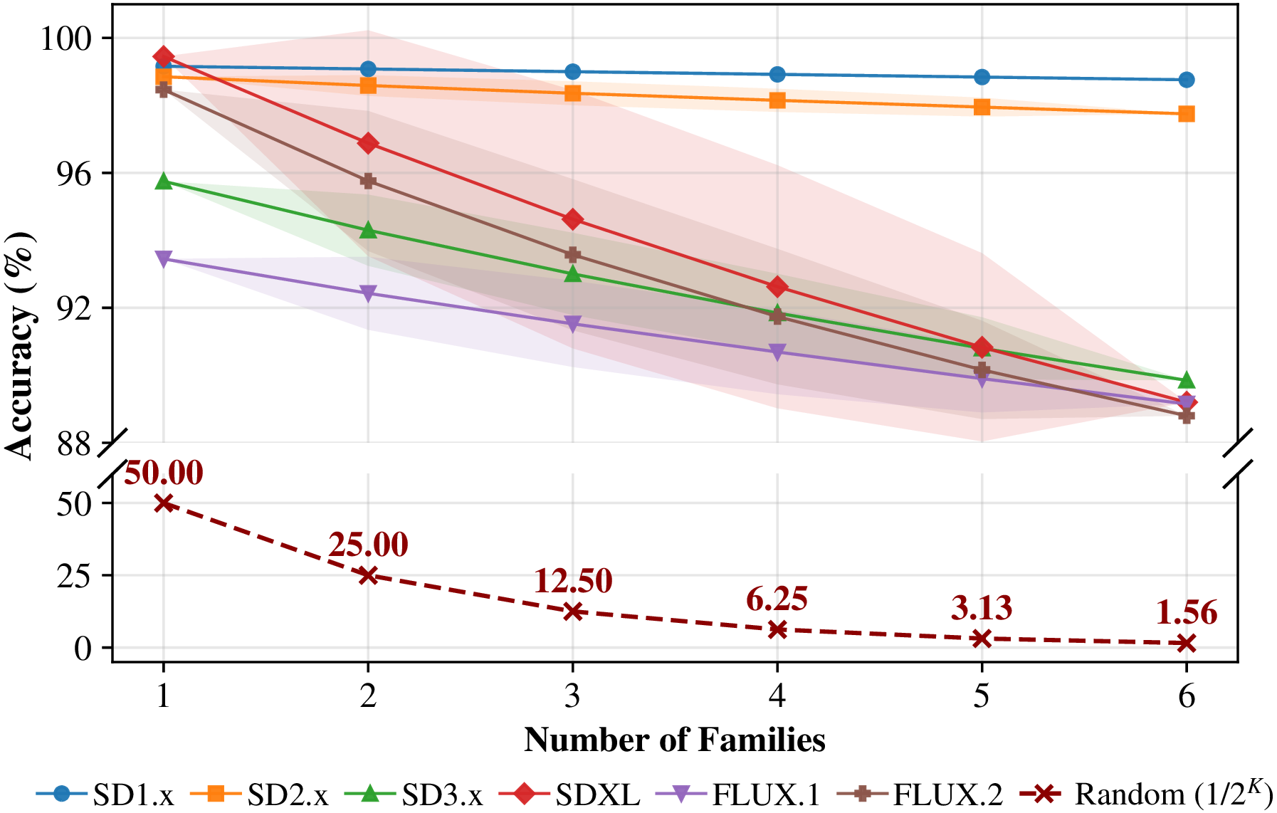
Due to the two-stage decoupling, increasing the number of candidate families \(K\) affects only Stage 1. We vary \(K\) from 1 to 6 and enumerate all \(\binom{6}{K}\) family subsets for each \(K\), recording the Stage 1 accuracy under each subset, as shown in Fig. 6. As \(K\) increases, attribution accuracy decreases moderately but remains well above the random baseline (\(1/2^K\)). SD1.x and SD2.x are the most stable, maintaining accuracy above 97% with drops of at most 1.1%. Other families are more sensitive to increasing \(K\), with drops of approximately 5%-10%. Even in the most challenging \(K{=}6\) setting, all families maintain accuracy above 88%.
| Family | Number of within-family variants \(J\) | ||||
|---|---|---|---|---|---|
| 2-6 | 1 | 2 | 3 | 4 | 5 |
| SD1.x | 100.00 \(\pm\) 0.0 | 98.54 \(\pm\) 2.1 | 97.25 \(\pm\) 2.2 | 96.11 \(\pm\) 1.8 | 95.08 \(\pm\) 0.0 |
| SD2.x | 100.00 \(\pm\) 0.0 | 99.47 \(\pm\) 0.7 | 98.98 \(\pm\) 0.6 | 98.55 \(\pm\) 0.0 | – |
| SD3.x | 100.00 \(\pm\) 0.0 | 98.53 \(\pm\) 2.4 | 97.15 \(\pm\) 2.2 | 95.80 \(\pm\) 0.0 | – |
| SDXL | 100.00 \(\pm\) 0.0 | 98.62 \(\pm\) 0.8 | 97.75 \(\pm\) 0.7 | 97.00 \(\pm\) 0.0 | – |
| FLUX.1 | 100.00 \(\pm\) 0.0 | 99.53 \(\pm\) 0.4 | 99.37 \(\pm\) 0.2 | 99.30 \(\pm\) 0.0 | – |
| FLUX.2 | 100.00 \(\pm\) 0.0 | 94.87 \(\pm\) 3.3 | 92.40 \(\pm\) 0.0 | – | – |
2.5pt
7.3.2 Within-family variant scaling↩︎
Increasing the number of within-family variants \(J\) affects only Stage 2. We progressively increase \(J\) from 1 to the maximum family size, enumerate all possible model subsets of size \(J\), and report the mean Stage 2 accuracy, as shown in Tab. 6. Accuracy remains high as \(J\) grows, although attribution naturally becomes more challenging with more candidate variants: SD2.x and FLUX.1 retain 98.55% and 99.30% at their maximum sizes, respectively. FLUX.2 shows the largest degradation as \(J\) increases, yet still achieves 92.40% with all three candidate variants. Both scaling experiments confirm that DNA maintains stable attribution performance as the candidate space expands along both the inter-family and intra-family dimensions.
7.4 sec:Efficiency↩︎
| OCC-CLIP | De-Fake-Img | De-Fake-Hyb | LatentTracer | DNA | ||||||
|---|---|---|---|---|---|---|---|---|---|---|
| (l2ptr2pt)2-3 (l2ptr2pt)4-5 (l2ptr2pt)6-7 (l2ptr2pt)8-9 (l2ptr2pt)10-11 | ||||||||||
| SD1.x | 0.131 | 0.048 | 0.182 | 0.032 | 1.205 | 0.159 | 117.7 | 27.28 | 0.107 | 15.82 |
| SD2.x | 0.043 | 0.033 | 0.179 | 21.56 | 1.031 | |||||
| SD3.x | 0.046 | 0.030 | 0.162 | 96.90 | 32.67 | |||||
| SDXL | 0.049 | 0.030 | 0.152 | 139.5 | 5.266 | |||||
| FLUX.1 | 0.043 | 0.031 | 0.157 | 95.62 | 28.13 | |||||
| FLUX.2 | 0.044 | 0.032 | 0.164 | 71.65 | 86.68 | |||||
| Acc(%) | 5.48 | 39.76 | 9.09 | 48.09 | 11.45 | 59.90 | 23.85 | 26.62 | 92.25 | 96.36 |
2pt
Table 7 reports the per-image inference time of each method on DNA-30K. In Stage 1, DNA requires only 0.107s per image, faster than all baselines, because AEDR uses only two VAE forward passes and requires neither backbone access nor gradient optimization. In Stage 2, DNA ranges from 1.031s (SD2.x) to 86.68s (FLUX.2), which is higher than supervised methods such as OCC-CLIP and De-Fake (both under 0.2s) but is faster than LatentTracer on five families while achieving substantially higher attribution accuracy. Given that DNA achieves 96.36% Stage 2 accuracy compared to 26.62% for LatentTracer, this computational cost reflects a favorable accuracy–efficiency trade-off. The Stage 2 runtime is mainly determined by the number of forward passes across timesteps and noise samples, and can be reduced by decreasing \(L^{\star}\) or \(S\) when computational resources are limited, trading a modest accuracy degradation for a significant speedup (see Fig. 7).
7.5 Robustness↩︎
lllc ccc Family & Scheduler & Configuration & Steps & Stage 1 & Stage 2 & End-to-End
& EulerDiscrete (Default) & Guidance scale = 7.5 & 40 & 89.20 & 97.00 & 87.05
& DDIM & Guidance scale = 7.5 & 50 & 90.85 & 96.15 & 87.90
& EulerDiscrete & Guidance scale = 7.5 & 30 & 89.20 & 96.75 &
& EulerAncestralDiscrete & Guidance scale = 7.5 & 30 & 89.75 & 94.55 &
& DPMSolverMultistep & Guidance scale = 7.5, Karras \(\sigma\) & 25 & 86.90 & 96.50 & 84.25
& FlowMatchEuler (Default) & Guidance scale = 3.5, Dynamic shift & 50 & 89.15 & 99.30 & 88.60
& FlowMatchEuler & Guidance scale = 3.5, Fixed shift = 3.0 & 30 & 88.20 & 99.10 &
& FlowMatchEuler + Beta \(\sigma\) & Guidance scale = 3.5, Fixed shift = 3.0 & 30 & 91.70 & 99.50 & 91.30
& FlowMatchEuler + Karras \(\sigma\) & Guidance scale = 3.5, Fixed shift = 3.0 & 30 & 88.60 & 98.40 &
7.5.1 Robustness to sampling configurations↩︎
To verify that DNA is robust to changes in generation-time sampling configurations, we conduct experiments on two representative families: SDXL (denoising diffusion) and FLUX.1 (flow matching). For SDXL, we replace the default EulerDiscrete scheduler with DDIM, EulerAncestralDiscrete, and DPMSolverMultistep. For FLUX.1, since the Rectified Flow path is tightly coupled with the FlowMatchEuler solver, we instead vary key configurations within this framework, including dynamic/fixed shift and \(\sigma\)-schedule forms (linear, Beta, Karras).
As shown in Tab. ¿tbl:Rob95Scheduler?, the end-to-end accuracy of SDXL under 4 alternative schedulers ranges from 84.25% to 87.90%; FLUX.1 across three configurations ranges from 87.45% to 91.30%, with fluctuations of no more than 3% compared to the default configuration. Notably, Stage 2 accuracy remains above 94.55% across all configurations, suggesting that NPC captures an intrinsic prediction-consistency signal governed primarily by the training objective and backbone parameters, rather than by the specific sampling configuration.
| Family | Number of Calibration Samples (per model) | ||||||
|---|---|---|---|---|---|---|---|
| (l1ptr1pt)2-8 | 100 | 80 | 60 | 40 | 20 | 10 | 5 |
| SD1.x | 93.92 | 92.20 | 92.76 | 93.12 | 89.44 | 88.56 | 87.92 |
| SD2.x | 96.40 | 95.15 | 96.90 | 95.60 | 94.65 | 89.25 | 90.25 |
| SD3.x | 86.30 | 86.15 | 86.40 | 87.90 | 85.10 | 77.40 | 82.80 |
| SDXL | 87.05 | 77.00 | 77.75 | 77.90 | 73.70 | 72.25 | 73.35 |
| FLUX.1 | 88.60 | 91.10 | 90.75 | 88.85 | 86.00 | 84.25 | 81.30 |
| FLUX.2 | 82.40 | 80.27 | 81.87 | 82.33 | 74.47 | 70.53 | 83.87 |
| Average | 89.11 | ||||||
4pt
7.5.2 Robustness to limited calibration samples↩︎
We progressively reduce the calibration budget per model from the default 100 samples to 5. We re-estimate the Stage 1 thresholds, Stage 2 discriminative timesteps, and normalized calibrated scores, and evaluate end-to-end performance on the test set, as shown in Tab. 8. When the sample count decreases from 100 to 40, the average accuracy drops by only 1.49% (89.11%\(\to\)87.62%). Even under the extreme 5-sample setting, end-to-end accuracy remains at 83.25%. Performance is not strictly monotonic with the sample count, which may arise from variations in calibration-sample composition and their effects on threshold estimation and timestep selection. Nevertheless, the overall trend is stable, indicating that DNA is not overly sensitive to calibration-set size and maintains useful performance under limited annotation budgets.
| Method | Ideal (Clean) | Real-World (JPEG) | ||||
|---|---|---|---|---|---|---|
| (l3ptr3pt)2-4 (l3ptr3pt)5-7 | Stage 1 | Stage 2 | E2E | Stage 1 | Stage 2 | E2E |
| OCC-CLIP | 10.35 | 48.60 | 7.35 | 6.30 | 45.90 | 4.60 |
| De-Fake-Img | 9.90 | 45.30 | 7.90 | 44.70 | 7.65 | |
| De-Fake-Hyb | 7.80 | 7.00 | 8.95 | 7.70 | ||
| LatentTracer | 1.80 | 24.10 | 0.30 | 0.00 | 24.75 | 0.00 |
| DNA | 97.75 | 98.55 | 96.40 | 9.55 | 82.05 | |
| DNA-DCT | 98.55 | 44.20 | 82.05 | 34.60 | ||
4pt
7.5.3 Robustness in real-world settings↩︎
We evaluate attribution performance under real-world dissemination conditions using the SD2.x family as a representative stress test beyond the clean auditing setting. A common real-world scenario is image dissemination through social media platforms, where uploaded images are often recompressed by services such as Facebook and Instagram. To approximate this process in a controlled manner, we conduct large-scale experiments using JPEG compression with QF=75. As shown in Tab. 9, all methods experience varying degrees of performance degradation after compression, while DNA achieves the highest end-to-end accuracy. The stage-wise results further identify the primary source of degradation: NPC retains an accuracy of 82.05%, whereas the pixel-level attribution signals used by AEDR are more sensitive to compression artifacts.
To improve Stage 1 robustness, we transfer the AEDR statistic from the pixel domain to the DCT frequency domain. We apply an orthogonal DCT to non-overlapping \(8\times8\) blocks of the two reconstruction residuals, aggregate the coefficients by radial frequency, and compute the attribution statistic from the energy ratio of the middle- and high-frequency bands. The same formulation is applied to all six families, with family-specific thresholds re-estimated on the calibration set and the original unique-acceptance rule retained. As shown in Tab. 9, the DCT-based variant (DNA-DCT) improves Stage 1 accuracy from 9.55% to 44.20% and end-to-end accuracy from 9.15% to 34.60%, with only a slight reduction under clean conditions. We further conduct a pilot evaluation by uploading 100 randomly sampled images to Facebook and evaluating the downloaded versions. The 100 images are sampled uniformly from the four SD2.x variants; the downloaded images are evaluated without additional processing. In this setting, DNA-DCT improves end-to-end accuracy from 3% to 31%. These results suggest that frequency-domain statistics can partially mitigate platform recompression and provide a promising direction for improving Stage 1 robustness (see Sec. 8).
7.6 Ablation Studies↩︎
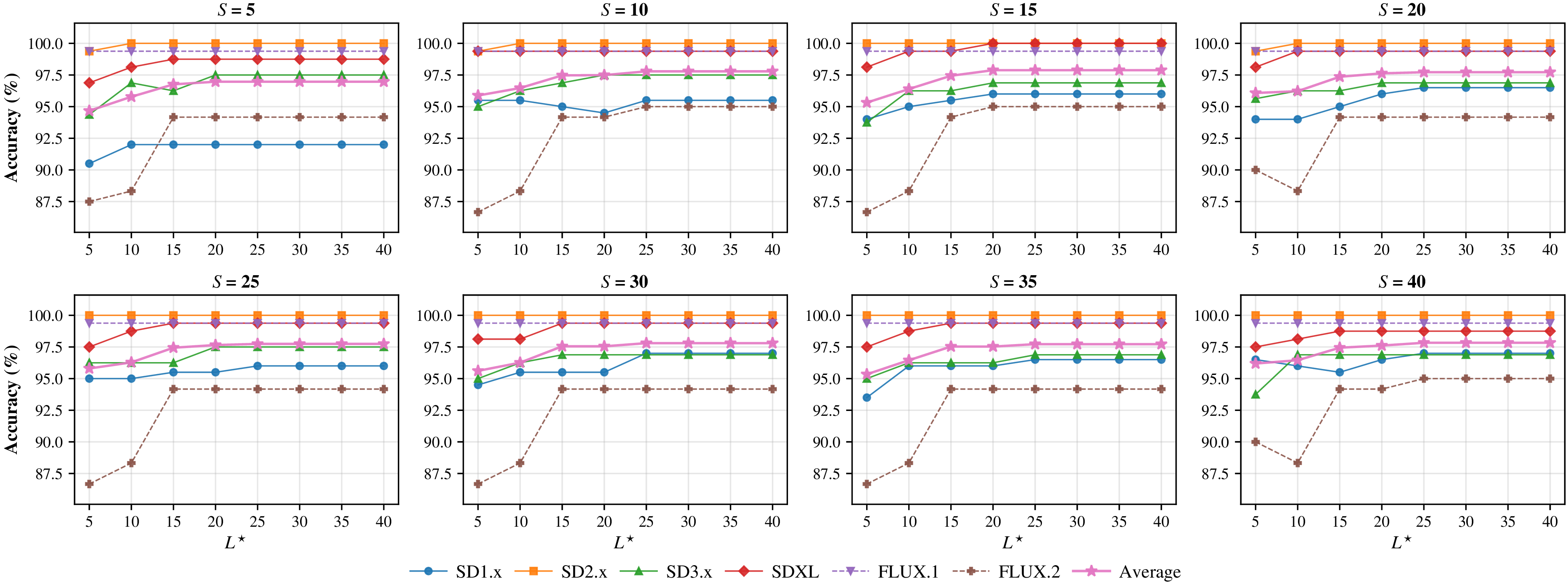
| Family | \(L^{\star}\) | \(S\) | Cal Acc (%) | Val Acc (%) | Test Acc (%) |
|---|---|---|---|---|---|
| SD1.x | 25 | 30 | 96.00 | 97.00 | |
| SD2.x | 5 | 10 | 99.17 | 100.00 | |
| SD3.x | 5 | 20 | 95.83 | 97.50 | |
| SDXL | 10 | 5 | 98.75 | 99.38 | |
| FLUX.1 | 5 | 5 | 100.00 | 99.38 | |
| FLUX.2 | 5 | 25 | 93.89 | 94.17 | |
| Average | – | – | 97.27 | 97.91 |
3.5pt
7.6.1 Noise samples and discriminative timesteps↩︎
NPC involves two key hyperparameters: the number of noise samples \(S\) and the number of discriminative timesteps \(L^{\star}\). We split the 100 calibration images per model into a 60/40 calibration/validation partition and evaluate Stage 2 accuracy on the validation set over a two-dimensional grid \(S, L^{\star}\in\{5,10,\dots,40\}\), as shown in Fig. 7. Overall, the average accuracy ranges from 94.67% to 97.88%, indicating that NPC is not sensitive to either hyperparameter. Per-family results show that SD2.x and FLUX.1 are the most stable, with accuracy consistently above 99%. FLUX.2 is relatively more sensitive, dropping to approximately 86.67% at low \(S\) and low \(L^{\star}\), but recovering to about 95% as both increase. The general trend indicates that accuracy saturates beyond \(S,L^{\star}\geq 15\), with further increases primarily adding linear inference overhead. Based on the performance–efficiency trade-off, the final per-family configurations are listed in Tab. 10. After transferring the parameters selected on the validation set to the test set, the average accuracy decreases from 97.91% to 96.36%, with the largest per-family drop not exceeding 2.38%.
| Family | Base | +Hom. | +Shared | +Sem. | +DisStep | +Norm. | Final |
|---|---|---|---|---|---|---|---|
| SD1.x | 50.40 | +0.12 | +12.40 | +26.72 | +2.52 | +1.76 | |
| SD2.x | 54.95 | +2.90 | +5.95 | +25.55 | +0.90 | +6.15 | |
| SD3.x | 50.95 | +2.15 | +4.80 | +11.85 | +8.85 | +7.70 | |
| SDXL | 34.30 | +5.35 | +8.05 | +26.10 | +4.40 | +8.85 | |
| FLUX.1 | 43.20 | +13.30 | +1.65 | +19.65 | +3.25 | +7.55 | |
| FLUX.2 | 37.53 | +8.74 | +5.00 | +12.00 | +10.60 | +8.53 | |
| Average | 45.22 | ||||||
2pt
7.6.2 Component ablation↩︎
To assess the contribution of each component in DNA, we incrementally add five core components and report the end-to-end attribution accuracy gain at each step, as shown in Tab. 11. The Base configuration uses the uncalibrated AEDR ratio for Stage 1 and raw native prediction-error aggregation for Stage 2, achieving an average end-to-end accuracy of 45.22%. On top of this, homogeneity calibration (+Hom.), shared noise perturbation (+Shared), semantic conditioning (+Sem.), discriminative timestep selection (+DisStep), and normalized calibrated scoring (+Norm.) yield gains of 5.43%, 6.31%, 20.31%, 5.09%, and 6.76%, respectively, ultimately raising the accuracy to 89.11%—a cumulative improvement of 43.89%. Semantic conditioning yields the largest incremental gain (+20.31%), indicating that aligning the conditioning input with the generation-stage semantics allows prediction error differences to more accurately reflect distributional shifts among candidate models. The full component configuration yields consistent improvements across all families, suggesting that the component designs are not tied to the statistical characteristics of a single family.
| Family | \(J\) | Original | Semantic | Generic | None | Random |
|---|---|---|---|---|---|---|
| SD1.x | 5 | 97.16 | 95.08 | 73.60 | 65.52 | 20.00 |
| FLUX.1 | 4 | 99.75 | 99.30 | 91.80 | 88.40 | 25.00 |
3pt
7.6.3 Effect of semantic conditioning↩︎
To examine what drives the large gain from semantic conditioning (+20.31% in Tab. 11), we evaluate Stage 2 accuracy under four conditioning strategies on SD1.x (denoising diffusion) and FLUX.1 (flow matching), as shown in Tab. 12. Both families exhibit a consistent ordering: Original \(\approx\) Semantic \(\gg\) Generic \(>\) None \(\gg\) random. Original and Semantic differ by less than 2.1% on both families, suggesting that BLIP-2 captions provide an effective deployment-time proxy for the true generation prompt. Crucially, None still far exceeds random (65.52% vs.% for SD1.x; 88.40% vs.% for FLUX.1), indicating an intrinsic backbone signal independent of semantic input and arguing against a pure caption–image alignment explanation. Correct image-specific conditioning amplifies this intrinsic signal, with the amplification scaling with variant difficulty: a 29.6% gain from None to Semantic for closely related SD1.x variants, compared with 10.9% for the more distinct FLUX.1.
8 Limitations and Future Work↩︎
Robustness of Family-Level Screening. As shown in Sec. 7.5, the end-to-end robustness of DNA to image recompression is primarily limited by Stage 1, whereas Stage 2 remains comparatively stable. This difference arises because AEDR relies on VAE reconstruction statistics that are directly affected by compression artifacts, while NPC measures relative native-prediction consistency among within-family backbones and is empirically less sensitive to such pixel-level distortions. To alleviate this limitation, we replace the original pixel-domain statistic with a DCT-based frequency-domain metric, which substantially improves both Stage 1 and end-to-end accuracy under controlled JPEG recompression and for images recompressed by Facebook. Nevertheless, the resulting end-to-end accuracy reaches only 34.60% under JPEG compression and 31% in the Facebook pilot evaluation, indicating that robust family-level screening under real-world platform recompression remains an open challenge. Since Stage 1 is methodologically decoupled from NPC (see Sec. 5), future work may incorporate platform-aware calibration, compression-invariant reconstruction statistics, or adaptive spatial–frequency representations without modifying Stage 2.
| SD1.x | SD2.x | SD3.x | SDXL | FLUX.1 | FLUX.2 | Avg | |
|---|---|---|---|---|---|---|---|
| AUROC | 0.725 | 0.745 | 0.509 | 0.688 | 0.687 | 0.553 | 0.651 |
| Rej@95% | 21.1 | 31.2 | 9.6 | 12.3 | 34.3 | 13.1 | 20.3 |
| Known | 96.0 | 98.4 | 84.0 | 96.6 | 99.0 | 84.3 | 93.1 |
3.5pt
Toward Within-Family Open-Set Attribution. Within a confirmed family, DNA currently performs closed-set attribution and assumes a complete candidate set. To probe the rejection of unknown within-family variants, we conduct a leave-one-out (LOO) experiment: one variant per family is held out as unknown, while NPC statistics are re-estimated on the remaining known variants. Table 13 reports 3 metrics averaged over all LOO folds. The average AUROC of 0.651 and rejection rate of 20.3% indicate partial but insufficient rejection capability. Per-fold analysis reveals that each family contains at least one highly similar variant whose consistency profile is difficult to distinguish from known candidates. Notably, closed-set classification on known variants remains above 84% even in the LOO setting, suggesting that NPC’s discriminative power is largely preserved when the candidate set shrinks.
9 Conclusion↩︎
This paper proposes Dual-stage Native Attribution (DNA), a coarse-to-fine framework that decouples source-model attribution along the “VAE\(\rightarrow\)backbone” hierarchy into open-set family-level screening and closed-set model-level attribution. The fine-grained stage introduces Native Prediction Consistency (NPC), which supports both denoising diffusion and flow matching. We construct DNA-30K, comprising 30,000 images from 24 candidate models across six families, together with unknown-source images for open-set family-level evaluation. On DNA-30K, DNA achieves 92.25% Stage 1 accuracy, 96.36% Stage 2 accuracy under the oracle true-family setting, and 89.11% end-to-end attribution accuracy, outperforming the strongest AEDR-enhanced baseline by 33.81%. DNA remains stable under candidate-set expansion, diverse sampling configurations, and limited calibration data, retaining 83.25% end-to-end accuracy with only five calibration images per model.
References↩︎
Chao Wang, Kejiang Chen, Zijin Yang, Yuang Qi, Weiming Zhang and Nenghai Yu are with the University of Science and Technology of China, Hefei, China; Yaofei Wang is with Hefei University of Technology, Hefei, China. (Email: chaowang0708@mail.ustc.edu.cn, chenkj@ustc.edu.cn, zhangwm@ustc.edu.cn)↩︎
Corresponding authors: Kejiang Chen and Weiming Zhang↩︎
Our source code is available at https://github.com/wangchao0708/DNA.↩︎