Calibrated Closed-Form Uncertainty for Radiative Gaussian Splatting in Sparse-View CT
July 15, 2026
Abstract
Radiative Gaussian splatting has made sparse-view CT reconstruction fast, but existing methods output point estimates with no notion of where the reconstruction can be trusted. We exploit a property of transmissive X-ray imaging that RGB splatting cannot claim — projection and voxelization are strictly linear in the per-Gaussian densities — to equip radiative Gaussians with a variational density posterior whose predictive variance propagates in closed form, exactly, in a single forward pass, in both volume space (\(\sigma^2(x)=\sum_i g_i(x)^2 s_i^2\)) and projection space (\(\mathrm{Var}[I_p]=\sum_i w_{i,p}^2 s_i^2\)). We present the first systematic calibration study for Gaussian-splatting CT (Spearman / AUSE / ECE with temperature scaling), showing that the resulting per-voxel uncertainty ranks true reconstruction error on 14 of 15 scenes of the official benchmark across three view budgets — 9 of 15 additionally meeting our magnitude-calibration target after a single temperature — while the perturbation-ensemble heuristic of concurrent work, transplanted to voxel space under the same protocol on our development scenes, does not (rank correlation as low as \(-0.08\)). We then dissect why uncalibrated acquisition scores can nevertheless select acceptable views, identifying three regimes — flat (isotropic, balanced), pathological (degenerate coverage), and anisotropic — and showing, in controlled single-scene testbeds, that principled uncertainty earns a measurable premium only in the last, motivating a coverage-gated, maturity-scheduled acquisition policy; the same calibrated posterior further points toward a dose-adaptive stopping rule, whose experimental validation we leave to future work.
1 Introduction↩︎
Sparse-view computed tomography (CT) reduces patient dose by acquiring few X-ray projections, at the cost of an ill-posed inverse problem: with the angular sampling well below the Nyquist rate, large regions of the reconstruction are interpolated rather than measured. Radiative 3D Gaussian splatting — most prominently R2-Gaussian [1] — has made this regime fast and accurate, representing the attenuation field as a sum of anisotropic Gaussians and rendering it through a differentiable rasterizer. Yet every such method returns a single point estimate. It cannot say where the reconstruction is trustworthy and where it is a confident guess — precisely the question a clinician, or any downstream decision, must answer before acting on a sparse-view volume.
Uncertainty quantification is the natural remedy, but for Gaussian-splatting CT it is essentially unaddressed. The one concurrent effort in this space, the Perturbed Gaussian Ensemble of [2], uses ensemble disagreement purely as an acquisition score for next-best-view selection: it perturbs low-density Gaussians, measures projection-space SSIM variance across replicas, and never validates that this signal corresponds to reconstruction error, nor produces a per-voxel uncertainty map. The broader Gaussian-splatting uncertainty literature is confined to RGB rendering, where alpha compositing is highly nonlinear in opacity: closed-form variance propagation [3] is therefore approximate, calibration is rarely evaluated, and none of it targets the transmissive physics of X-ray. Calibrated CT uncertainty has been demonstrated only for implicit neural representations [4], not for Gaussian splatting.
Our starting point is a physical observation with an outsized consequence. Because X-rays are transmissive rather than reflective, both the rendered projection and the voxelized volume are strictly linear in the per-Gaussian densities — there is no alpha compositing, no view-dependent occlusion. This linearity is the enabling property of everything that follows. If we lift each density to a Gaussian posterior, the predictive variance of the reconstruction is a variance of a weighted sum of independent variables, which has an exact closed form. We show this closed form is computable by the unchanged rasterizer and voxelizer through a simple algebraic identity (squaring a Gaussian kernel halves its covariance), so that both volume-space and projection-space uncertainty come out of a single extra forward pass, with no CUDA changes and no sampling. The same identity makes the Monte-Carlo estimator of concurrent work a special case: instantiated with their perturbation distribution’s per-Gaussian variances, our one-pass expression evaluates exactly the quantity their ensemble variance approximates with finite samples.
Crucially, having a cheap, exact uncertainty is not the same as having a useful one. The central empirical contribution of this paper is to treat calibration — the correspondence between predicted uncertainty and true error — as a first-class deliverable, and to separate it cleanly from the acquisition task that has so far been used as its only proxy. We find the two come apart in an instructive way. Our variational posterior yields per-voxel uncertainty that tracks error well and, on most scenes, is repairable to good magnitude calibration by a single temperature — though five of fifteen official scenes resist a single global scalar (4.3); the perturbation heuristic, transplanted to voxel space under an identical protocol, does not — its rank correlation with error dips below zero on one scene, even though its temperature-scaled ECE looks acceptable, a textbook case for why calibration must be judged by rank and coverage metrics, not a single scalar. Yet the same heuristic does help view selection in its own experiments. Resolving this apparent paradox — an uncalibrated score that still selects acceptable views — leads to our second empirical contribution: a controlled dissection showing that view selection is a low-stakes decision except in identifiable regimes (degenerate coverage, and genuinely anisotropic content), that in the degenerate-coverage regime the heuristic largely functions as a coverage detector, which a free geometric rule can replace at no cost, and that its own schedule queries the score when the model is least mature. These findings prescribe an acquisition policy rather than a new score, which we instantiate and evaluate.
1.0.0.1 Contributions.
Exact closed-form uncertainty for radiative Gaussians. We lift per-Gaussian densities to a variational posterior and derive the exact predictive variance in both volume and projection space, computable by the unchanged rasterizer/voxelizer in a single forward pass. The strict linearity of X-ray rendering makes this propagation exact rather than approximate — a property RGB-domain splatting cannot claim — and subsumes the concurrent Monte-Carlo estimator: instantiated with its perturbation variances, the same identity evaluates that estimator’s infinite-sample limit exactly ([sec:method-linearity] [sec:closed-form]).
The first systematic calibration study for Gaussian-splatting CT. Using Spearman, AUSE, and post-hoc-temperature ECE with a held-out fit/evaluation split, we quantify per-voxel uncertainty quality against ground-truth error across 15 official scenes at three view budgets, benchmarking our variational posterior against a deep-ensemble upper bound and against the concurrent perturbation heuristic transplanted to voxel space ([sec:calibration-protocol] [sec:threeway] [sec:main-table]).
A mechanism account of when uncertainty helps acquisition. On controlled testbeds we characterize three view-selection regimes and show, with a view-level oracle, closed-loop four-arm study, and per-round schedule autopsy, that principled uncertainty earns a premium over free geometry only under anisotropic content — establishing that calibrated quantification and view selection are separable products ([sec:why-uncalibrated] [sec:ssim]).
Coverage-gated, calibrated acquisition (CGCA). We turn the mechanism findings into a policy — guarantee coverage geometrically, score only on converged models, and spend a hyperparameter-free closed-form score where it earns a premium — and show it matches the concurrent heuristic’s acquisition gains at roughly one-tenth the scoring cost while, unlike any ranking heuristic, sharing a posterior that also supplies calibrated maps and points toward a dose-adaptive stopping rule ([sec:cgca-method] [sec:cgca-results]).
2 Related Work↩︎
2.0.0.1 Active view selection for radiance fields and tomography.
Active view selection has been explored for natural-light radiance fields via Fisher information (FisherRF [5]) and ensemble disagreement (ActiveNeRF [6]), but these assume occlusion-bounded, view-dependent appearance and transfer poorly to the transmissive, isotropic physics of X-ray imaging; indeed, the diagonal-FIM approximation underlying FisherRF has been shown to degrade under the strong along-ray coupling of X-ray projection [2]. Most closely related, the concurrent Perturbed Gaussian Ensemble [2] selects X-ray views by stochastically scaling the densities of the lowest-density Gaussians and ranking candidates by the sample variance of projection-space SSIM across \(N{=}10\) perturbed replicas. Their uncertainty is validated only indirectly, through downstream reconstruction quality: neither arXiv version of their paper reports uncertainty–error correspondence metrics (Spearman, AUSE, ECE), quantitatively compares the predicted uncertainty against reconstruction error, or produces per-voxel volumetric uncertainty maps. In contrast, we treat calibrated, closed-form, per-voxel density uncertainty as a first-class deliverable. Their Eq. 8 is, moreover, the Monte-Carlo estimator of our closed-form expression instantiated with their perturbation distribution’s per-Gaussian variances; the same one-pass identity evaluates its infinite-sample limit exactly.
2.0.0.2 Uncertainty and closed-form variance in Gaussian splatting.
Closed-form variance compositing has appeared in RGB-domain splatting — VarSplat [3] propagates per-splat appearance variance through alpha compositing via the law of total variance, and VBGS [7] derives conjugate closed-form updates for continual learning — but nonlinear alpha blending renders such predictive propagation approximate, the closed form in VBGS refers to parameter updates rather than predictive-variance propagation, and neither work evaluates calibration. Bayesian and variational treatments of 3DGS for RGB rendering are now emerging: Horseshoe Splatting [8] places a global–local Horseshoe prior on per-splat covariance scales and reports calibrated pixel-wise uncertainty via factorized variational inference, and rendering-aware Bayesian 3DGS with a Normal-Inverse-Wishart posterior over Gaussian geometry [9] produces native predictive intervals and drives acquisition. Both are RGB methods whose uncertainty lives on geometry/appearance under nonlinear rendering; our posterior is over radiative density under strictly linear rendering, which is what makes our two-domain propagation exact rather than approximate, and our deliverable is per-voxel volumetric calibration for CT rather than per-pixel image uncertainty. Calibrated uncertainty for CT reconstruction has been demonstrated for implicit neural representations (UncertaINR [4]), not for Gaussian splatting.
2.0.0.3 A note on “closed-form” in X-ray Gaussian splatting.
The phrase closed-form has recently been used in this space for a different object: Exact-GS [10] and radioactive Gaussian ray tracing [11] derive closed-form/analytic projection integrals that remove the affine approximation of R2-Gaussian and improve rendering accuracy. Their closed form concerns the forward rendering of the mean field; ours concerns the propagation of a posterior variance. The two are orthogonal and composable: a more exact forward model would only sharpen the mean our variance is computed around. To the best of our knowledge, no prior work on X-ray/CT radiative Gaussian splatting equips per-Gaussian densities with explicit posterior distributions, propagates them to volume and projection space in closed form — which the strict linearity of X-ray rendering makes exact rather than approximate — or evaluates the calibration of the result.
3 Method↩︎
![Figure 1: Training and uncertainty pipeline. We extend R^2-Gaussian [1] with a variational density posterior \rho_i \sim \mathcal{N}(m_i, s_i^2) per Gaussian. Training renders reparameterized density samples through the unchanged rasterizer and applies a KL prior that anchors s_i where no ray constrains the density (Sec. 3.2). At evaluation, mean densities m_i define the reconstruction \bar{V}, and the \sqrt{2}-scaling identity turns the same rasterizer/voxelizer into an exact one-pass evaluator of the predictive variance in both projection and volume space (Sec. 3.3).](/article/2607.13682/figures/structure_example.png "fig:")
3.1 Preliminaries: radiative Gaussians are linear in density↩︎
We build upon R\(^2\)-Gaussian [1] (1), which represents the attenuation field as a sum of radiative Gaussians. Each kernel defines a local Gaussian-shaped density with learnable central density \(\rho_i\), position \(\mathbf{p}_i \in \mathbb{R}^3\), and covariance \(\boldsymbol{\Sigma}_i = \mathbf{R}_i \mathbf{S}_i \mathbf{S}_i^\top \mathbf{R}_i^\top\): \[\label{eq:density-field} D(\mathbf{x}) = \sum_{i=1}^{M} \rho_i \exp\!\Big(-\tfrac{1}{2}(\mathbf{x}-\mathbf{p}_i)^\top \boldsymbol{\Sigma}_i^{-1}(\mathbf{x}-\mathbf{p}_i)\Big).\tag{1}\] R\(^2\)-Gaussian rectifies the integration bias of standard 3D Gaussian splatting and provides differentiable X-ray rasterization \(\mathcal{R}\) and density voxelization \(\mathcal{V}\). The pixel value of a projection and the value at a voxel are strictly linear in the per-Gaussian densities: \[\label{eq:linear-render} I_p = \sum_i w_{i,p}\,\rho_i, \qquad V(\mathbf{x}) = \sum_i g_i(\mathbf{x})\,\rho_i,\tag{2}\] where \(g_i(\mathbf{x})\) is the (density-independent) three-dimensional Gaussian kernel and \(w_{i,p} = \mu_i\,\hat{G}_i(p)\) combines the two-dimensional screen-space kernel with the view-dependent integration factor \(\mu_i^2 = 2\pi \det(\tilde{\boldsymbol{\Sigma}}_i)/\det(\hat{\boldsymbol{\Sigma}}_i)\) from the EWA ray-space covariance [12]. Unlike RGB Gaussian splatting, where alpha compositing is highly nonlinear in opacity, Eq. 2 is a weighted sum—this linearity is the enabling property for closed-form uncertainty propagation in Sec. 3.3.
3.1.0.1 Backbone training.
We adopt the R\(^2\)-Gaussian initialization (FDK volume), adaptive clone/split/prune, and photometric objective \[\label{eq:r2-loss} \mathcal{L}_{\mathrm{R^2}} = \|I_r - I_m\|_1 + \lambda_{\mathrm{ssim}}\bigl(1 - \mathrm{SSIM}(I_r, I_m)\bigr) + \lambda_{\mathrm{tv}}\,\mathrm{TV}(\mathbf{V}_{\mathrm{tv}}),\tag{3}\] where \(I_r\) and \(I_m\) are rendered and measured projections and \(\mathbf{V}_{\mathrm{tv}}\) is a tiny voxel patch for total-variation regularization. Unless stated otherwise, all backbone hyperparameters follow the official release.
3.2 A variational posterior over densities↩︎
3.2.0.1 Partial Bayes over densities.
We lift each central density to a Gaussian posterior \(\rho_i \sim \mathcal{N}(m_i, s_i^2)\) while keeping positions and covariances as point estimates—a deliberate partial-Bayes choice. Density is the linear carrier of all outputs in Eq. 2 ; geometric ambiguity is partially absorbed into \(s_i\), and, in exchange, propagation in Sec. 3.3 remains closed-form. Means and standard deviations are parameterized as \(m_i = \mathrm{softplus}(\theta_i^m)\) and \(s_i = \mathrm{softplus}(\theta_i^s)\). The uncertainty parameter \(s_i\) is co-optimized with \(m_i\) and follows clone/split/prune during adaptive density control.
3.2.0.2 Training objective.
At each iteration we draw one reparameterized sample \(\tilde{\rho}_i = m_i + \epsilon_i s_i\), \(\epsilon_i \sim \mathcal{N}(0,1)\), clamp \(\tilde{\rho}_i \ge 0\) to enforce non-negative density, and render/voxelize with \(\tilde{\rho}_i\) in place of \(\rho_i\). Training minimizes the single-sample reparameterized, ELBO-inspired objective \[\label{eq:training-loss} \mathcal{L} = \sum_{\mathrm{views}} \Bigl[ \|\hat{I} - I^{\mathrm{obs}}\|_1 + \lambda_d \bigl(1 - \mathrm{SSIM}(\hat{I}, I^{\mathrm{obs}})\bigr) \Bigr] + \lambda_{\mathrm{tv}}\,\mathrm{TV} + \lambda_{\mathrm{KL}}\, \overline{\mathrm{KL}}\!\bigl(\mathcal{N}(m_i,s_i^2)\,\|\,\mathcal{N}(0,\sigma_0^2)\bigr),\tag{4}\] with \(\lambda_{\mathrm{KL}}\) linearly warmed up over the first \(3{,}000\) iterations. We use \(\lambda_{\mathrm{KL}} = 10^{-3}\), \(\sigma_0 = 0.5\), and the R\(^2\)-Gaussian defaults for all remaining weights and schedules.
3.2.0.3 Role of the KL prior.
The KL term is not decorative. For Gaussians that no ray constrains—the null space of sparse-view tomography—the data term provides no gradient to \(s_i\), and the prior alone anchors \(s_i \approx \sigma_0\). This is precisely how “uncertain where unobserved” arises. Increasing \(\lambda_{\mathrm{KL}}\) from \(0\) to \(10^{-2}\) monotonically improves both rank-calibration metrics and pulls the raw uncertainty scale toward truth (Spearman \(0.643 \to 0.694\), AUSE \(0.371 \to 0.300\), raw ECE \(0.41 \to 0.15\); temperature-scaled ECE stays nearly flat; Table 5), confirming the mechanism. Final reconstructions and error maps use the posterior mean density \(m_i\); the small PSNR cost of variational training relative to R\(^2\)-Gaussian is quantified in Sec. 4.4.
3.3 Exact closed-form propagation, zero CUDA changes↩︎
3.3.0.1 Derivation.
Assuming independent \(\rho_i\), the variance of a linear combination yields, exactly, \[\label{eq:closed-form-var} \sigma^2(\mathbf{x}) = \sum_i g_i(\mathbf{x})^2 s_i^2, \qquad \mathrm{Var}[I_p] = \sum_i w_{i,p}^2 s_i^2.\tag{5}\] Eq. 5 is the predictive variance of the linear forward model; it is not an approximation to alpha-composited RGB splatting.
3.3.0.2 Implementation without CUDA changes.
Squaring a Gaussian kernel halves its covariance: \(g_i^2 = \exp\bigl(-\tfrac{1}{2}\mathbf{d}^\top (\boldsymbol{\Sigma}_i/2)^{-1}\mathbf{d}\bigr)\), i.e., scale \(\mathbf{S}_i \to \mathbf{S}_i/\sqrt{2}\).
Volume domain (B2-vol). One voxelizer pass with \((\mathbf{S}_i/\sqrt{2},\, s_i^2)\) returns \(\sigma^2(\mathbf{x})\) exactly.
Projection domain (B2-proj). Under the \(\sqrt{2}\) scaling, \(\mu_i \to \mu_i/\sqrt{2}\); one rasterizer pass with \((\mathbf{S}_i/\sqrt{2},\, \sqrt{2}\,\mu_i s_i^2)\) returns \(\sum_i w_{i,p}^2 s_i^2\) exactly.
Rasterizers cull negligible contributions; because rendering is linear in density, we pre-scale the variance channel into the nominal dynamic range and divide the output back—an exact rescaling.
3.3.0.3 Monte Carlo reference (B1).
We also estimate \(\sigma^2(\mathbf{x})\) with \(S\) reparameterized density samples using the same clamping as training. Without clamping, this converges to Eq. 5 as \(S \to \infty\). With clamping, B1 tracks the truncated predictive distribution used at train time and calibrates systematically better than the closed form (Sec. [sec:experiments-calibration]). Headline calibration metrics in Sec. [sec:experiments-p4] use B1 with \(S{=}16\); B2 is the single-pass deployment path for CGCA and efficiency ablations (\(2.5\)–\(10.4\times\) faster; volume Pearson \(0.80\)–\(0.88\) and projection Pearson \(0.94\)–\(0.95\), scene means over views, vs.MC; Table 4).
3.4 Calibration protocol↩︎
We evaluate whether predictive uncertainty \(\sigma(\mathbf{x})\) tracks the voxel-wise reconstruction error \(e(\mathbf{x}) = |\bar{V}(\mathbf{x}) - V_{\mathrm{gt}}(\mathbf{x})|\), where \(\bar{V}\) is the mean-density reconstruction from Sec. 3.2. Unless noted (CGCA scores, closed-form ablation), volume calibration uses B1 (\(S{=}16\) MC) maps; \(\tau\) is refit offline from stored mean/variance volumes under the grid below. Three complementary metrics are reported:
3.4.0.1 Spearman \(\rho\).
Rank correlation between \(\sigma(\mathbf{x})\) and \(e(\mathbf{x})\)—does high uncertainty co-locate with high error? Spearman is invariant to monotone rescaling and cannot be repaired post hoc.
3.4.0.2 AUSE.
Area under the sparsification curve when removing voxels in descending \(\sigma\) order; lower is better. AUSE measures whether discarding the most uncertain voxels reduces RMSE toward the oracle curve.
3.4.0.3 ECE with temperature scaling.
Regression calibration of \(\tau\sigma(\mathbf{x})\) against \(e(\mathbf{x})\). A global scalar \(\tau\) can repair magnitude without fixing spatial ordering; we therefore never report ECE alone.
3.4.0.4 Split-holdout temperature fitting.
For each scene we subsample \(10\%\) of evaluation voxels (fixed RNG seed), split them \(50/50\), and hold out the second half for reporting. Temperature \(\tau\) is chosen by grid search on the fit half over \(104\) log-spaced values on \([0.05,\,1000]\) (\({\approx}10\%\)
multiplicative resolution). Scaled ECE is reported on the disjoint holdout half only, so the reported value is never an in-sample minimum. We refer to this protocol as split_holdout. At grid resolution, \(\tau\) is often identical or near-identical across seeds within a scene, though a few scenes exhibit secondary \(\tau\) basins across seeds (Sec. [sec:experiments-p4], 7); cross-scene transfer remains untested. No fitted \(\tau\) reached the grid upper bound in
our runs (maximum observed: \(109.5\) for B1, \(749.4\) for B2).
3.4.0.5 Why three metrics.
They capture non-redundant failure modes: a global temperature can reduce ECE without improving spatial ranking—on head, the perturbation heuristic reaches holdout scaled ECE \(=0.104\) yet Spearman \(=-0.08\) (Sec. [sec:experiments-calibration], Table 1). Conversely, several official scenes pass Spearman but not ECE after scaling (Sec. [sec:experiments-p4]). We therefore never report ECE alone.
3.5 CGCA: coverage-gated, calibrated acquisition↩︎
![Figure 2: Coverage-gated calibrated acquisition (CGCA). Phase 1 (model-free): while the maximum uncovered arc exceeds the gate threshold \gamma, acquire the midpoint of the largest gap — degenerate clustering, the only catastrophic failure mode, is prevented geometrically. Phase 2 (calibrated): once coverage is secured, retrain to convergence on the acquired set and pick the candidate maximizing the one-pass closed-form projection variance \sum_p \mathrm{Var}[I_p] (Eq. 6 ); a coverage fallback re-engages the gate if the argmax would reopen a super-threshold gap.](/article/2607.13682/figures/CGCA_example.png "fig:")
Mechanism experiments (Sec. [sec:experiments-mechanism]) show that (i) degenerate angular clustering is the dominant failure mode (\(-2.6\) dB), (ii) querying scores on immature models yields noise, and (iii) uncertainty scores earn a measurable premium only in anisotropic regimes. Coverage-gated calibrated acquisition (CGCA; 2) turns these observations into a policy rather than a new heuristic score.
3.5.0.1 Coverage gate (model-free).
Let \(\mathcal{A}\) denote the set of acquired view angles and \(\mathrm{gap}(\mathcal{A})\) the maximum uncovered arc under the tomographic angular metric (views \(180^\circ\) apart are folded, as they constrain the same rays). While \(\mathrm{gap}(\mathcal{A}) > \gamma\), with \(\gamma = 2\times\) the uniform spacing at the target budget, the policy ignores all scores and acquires the midpoint of the largest gap. Degenerate clustering is the only large failure mode we observe, and its prevention must not depend on a learned signal.
3.5.0.2 Maturity schedule.
Scores are computed only on a model retrained to convergence on the current acquired set, never on a partially trained loop state. The schedule autopsy in Sec. [sec:experiments-mechanism] shows that the same score that is informative offline on a converged model is noise when queried during progressive training.
3.5.0.3 Calibrated closed-form score.
Once \(\mathrm{gap}(\mathcal{A}) \le \gamma\), the next view \(\theta\) maximizes the hyperparameter-free raw projection variance \[\label{eq:cgca-score} a(\theta) = \sum_p \mathrm{Var}\bigl[I_p(\theta)\bigr]\tag{6}\] from Eq. 5 , requiring one forward pass per candidate. A coverage fallback re-engages the gate if the argmax would reopen a super-threshold gap. We deliberately avoid the D-optimal diagonal form \(\sum_p \log\bigl(1 + \mathrm{Var}[I_p]/\sigma_n^2\bigr)\): with a misspecified noise floor \(\sigma_n\) the logarithm saturates and ranking degenerates to variance footprint size—a failure mode we document in Sec. [sec:experiments-cgca].
3.5.0.4 Scope.
The same calibrated posterior in principle supplies a dose-adaptive stopping rule (stop when \(\tau\sigma(\mathbf{x})\) falls below a clinical threshold); we state this as a design implication and leave experimental validation to future work. In this paper CGCA is evaluated on a circular-orbit testbed (Sec. [sec:experiments-cgca]); extension to hemispherical pose pools requires a spherical coverage metric and is future work.
4 Experiments↩︎
4.1 Setup↩︎
We evaluate on the X-Gaussian development scenes [13] (chest, abdomen, head; 50-view circular half-scans, trained on sparse subsets) and the R\(^2\)-Gaussian official 15-scene synthetic benchmark [1] (\(512^2\) projections, \(256^3\) volumes). Unless noted, variational models train for 10k iterations with \(\lambda_{\mathrm{KL}}{=}10^{-3}\), \(\sigma_0{=}0.5\), and a 3k-iteration KL warmup—identical across the development scenes and the official benchmark (a generalization test; no per-scene tuning).
4.1.0.1 Calibration protocol.
Volume calibration uses B1 Monte Carlo maps (\(S{=}16\) reparameterized samples with training-time clamping). Temperature \(\tau\) is fit on a 10% voxel subsample with
split_holdout over 104 log-spaced values on \([0.05,\,1000]\); scaled ECE is reported on the held-out half (Sec. 3.4). The same grid and protocol are applied to
every comparative method, including deep ensembles and the perturbation heuristic.
4.1.0.2 Gate criterion.
A scene passes if, at the 25-view budget, the 3-seed mean Spearman \(\ge 0.6\) and temperature-scaled ECE \(< 0.1\). All 75 official-benchmark runs complete on a single consumer GPU (RTX 4060 laptop, 8 GB; \(\approx\)6.4 minutes per run), and headline numbers use this machine under the wide-104 grid (9/15 pass); an independent replication on a second GPU (RTX 5080 laptop) yields 8/15 under the wide-80 grid, with cross-machine sensitivity confined to the scaled-ECE boundary band (8.3).
4.2 Per-voxel uncertainty quality: the three-way comparison↩︎
Table 1 places deep ensemble (\(K{=}5\)), variational MC (B1), variational closed-form (B2), and the perturbation heuristic under identical calibration rulers on the development set. Three metrics fail independently: on head, the perturbation heuristic reaches holdout ECE \(=0.104\) yet Spearman \(=-0.08\)—acceptable scaled magnitude with inverted spatial ranking. Variational MC tracks the ensemble on Spearman while closing most of the AUSE gap; B2 matches the ranking with a small calibration penalty (chest Spearman \(0.661\) vs.\(0.696\)). Multi-seed repeats (\(n{=}3\) per scene) give PSNR std \(\le 0.03\) dB and Spearman std \(\le 0.0007\); on these development scenes the fitted \(\tau\) is identical across seeds at grid resolution (\(\approx\)10% multiplicative steps), supporting fit-once-per-scene reuse — see 7 for official-benchmark scenes where this seed-stability fails.
| Scene | Method | Spearman | AUSE | ECE | \(\tau\) |
|---|---|---|---|---|---|
| Chest | Deep ensemble (\(K{=}5\)) | 0.723 | 0.269 | 0.221\(\to\)0.033 | 1.93 |
| Chest | Variational MC (B1) | 0.696 | 0.294 | 0.232\(\to\)0.082 | 3.78 |
| Chest | Perturbation heuristic | 0.485 | 0.663 | 0.430\(\to\)0.100 | 21.36 |
| Chest | Variational closed-form (B2) | 0.661 | 0.356 | 0.277\(\to\)0.088 | 5.05 |
| Abdomen | Deep ensemble (\(K{=}5\)) | 0.650 | 0.334 | 0.247\(\to\)0.031 | 2.34 |
| Abdomen | Variational MC (B1) | 0.600 | 0.376 | 0.181\(\to\)0.077 | 2.13 |
| Abdomen | Perturbation heuristic | 0.252 | 0.711 | 0.447\(\to\)0.131 | 50.76 |
| Abdomen | Variational closed-form (B2) | 0.567 | 0.419 | 0.183\(\to\)0.082 | 2.13 |
| Head | Deep ensemble (\(K{=}5\)) | 0.621 | 0.239 | 0.237\(\to\)0.030 | 2.34 |
| Head | Variational MC (B1) | 0.596 | 0.275 | 0.295\(\to\)0.066 | 3.44 |
| Head | Perturbation heuristic | \(-\)0.080 | 0.873 | 0.425\(\to\)0.104 | 19.41 |
| Head | Variational closed-form (B2) | 0.556 | 0.326 | 0.319\(\to\)0.121 | 4.17 |

4.3 Official 15-scene calibration main table↩︎
Table 2 extends the calibration study to all 15 official scenes and three view budgets (75 runs total). Gate: 9/15 pass under B1 MC and wide-104 \(\tau\) (25-view, 3-seed
mean). Fourteen of fifteen scenes exceed Spearman \(0.6\); the sole exception is 0_jaw_cone (Spearman \(\approx 0.23\)), consistent with an error floor: its error field is
nearly flat, with a \(p_{99}/p_{50}\) dynamic range of \(5.6\) (versus a median of \(86\) across passing scenes) and only 16% of the squared error carried by
the top-1% of voxels (versus 43%), so no spatial ordering of a near-constant field can score well. Five additional scenes fail only on ECE after global scaling—ranking is adequate but a single \(\tau\) cannot reconcile
spatially varying \(e/\sigma\) ratios (pancreas, kingsnake, mount, teapot, beetle). No fitted \(\tau\) reached the grid upper
bound (maximum observed: 109.5 for B1 on teapot_t75). B2 closed-form \(\sigma\) is uniformly worse on both Spearman and scaled ECE (75/75 pairwise wins for B1; 8.2),
motivating B1 for headline calibration while B2 remains the deployment path for CGCA (Sec. 5). Across the five completed machine\(\times\)grid combinations the gate count is \(\ge 8/15\) in four — the sole exception being the second machine under the legacy truncated grid — while three boundary-band scenes (chest, foot, kingsnake) flip pass/fail between machines; we therefore treat marginal-band
membership as machine-dependent and report per-seed temperatures (8.3, 7).
| scene | tier | PSNR3D | SSIM3D | Spearman | AUSE | scaled ECE | \(\tau\) (seed 0) | Gate |
|---|---|---|---|---|---|---|---|---|
| 0_chest_cone | 25 | 31.677\(\pm\)0.009 | 0.877\(\pm\)0.001 | 0.740\(\pm\)0.001 | 0.270\(\pm\)0.000 | 0.0986\(\pm\)0.0024 | 6.74 | \(✔\) |
| 50 | 34.110 | 0.920 | 0.723 | 0.298 | 0.0934 | 4.17 | ||
| 75 | 34.511 | 0.928 | 0.704 | 0.295 | 0.1041 | 4.17 | ||
| 0_foot_cone | 25 | 30.425\(\pm\)0.006 | 0.851\(\pm\)0.000 | 0.925\(\pm\)0.014 | 0.129\(\pm\)0.001 | 0.0863\(\pm\)0.0261 | 21.36 | \(✔\) |
| 50 | 31.593 | 0.868 | 0.872 | 0.138 | 0.0952 | 12.00 | ||
| 75 | 31.927 | 0.872 | 0.890 | 0.127 | 0.0974 | 12.00 | ||
| 0_head_cone | 25 | 35.735\(\pm\)0.029 | 0.946\(\pm\)0.000 | 0.744\(\pm\)0.001 | 0.234\(\pm\)0.000 | 0.0988\(\pm\)0.0016 | 4.17 | \(✔\) |
| 50 | 38.535 | 0.970 | 0.721 | 0.276 | 0.1014 | 3.12 | ||
| 75 | 39.112 | 0.974 | 0.710 | 0.286 | 0.1065 | 2.58 | ||
| 0_jaw_cone | 25 | 33.505\(\pm\)0.017 | 0.822\(\pm\)0.000 | 0.229\(\pm\)0.001 | 0.411\(\pm\)0.001 | 0.0509\(\pm\)0.0003 | 6.74 | \(\times\) |
| 50 | 35.873 | 0.872 | 0.210 | 0.432 | 0.0538 | 5.05 | ||
| 75 | 36.362 | 0.881 | 0.208 | 0.433 | 0.0548 | 4.59 | ||
| 0_pancreas_cone | 25 | 32.882\(\pm\)0.069 | 0.911\(\pm\)0.002 | 0.728\(\pm\)0.005 | 0.219\(\pm\)0.001 | 0.1081\(\pm\)0.0027 | 6.12 | \(\times\) |
| 50 | 35.905 | 0.946 | 0.703 | 0.243 | 0.1084 | 4.59 | ||
| 75 | 36.597 | 0.953 | 0.688 | 0.244 | 0.1040 | 3.79 | ||
| 1_beetle_cone | 25 | 39.266\(\pm\)0.031 | 0.989\(\pm\)0.000 | 0.908\(\pm\)0.002 | 0.022\(\pm\)0.007 | 0.1828\(\pm\)0.0281 | 28.51 | \(\times\) |
| 50 | 40.321 | 0.991 | 0.904 | 0.020 | 0.2260 | 0.31 | ||
| 75 | 40.373 | 0.991 | 0.905 | 0.015 | 0.1022 | 46.11 | ||
| 1_bonsai_cone | 25 | 32.612\(\pm\)0.018 | 0.906\(\pm\)0.001 | 0.917\(\pm\)0.004 | 0.150\(\pm\)0.005 | 0.0739\(\pm\)0.0244 | 12.00 | \(✔\) |
| 50 | 34.016 | 0.924 | 0.893 | 0.152 | 0.0539 | 12.00 | ||
| 75 | 34.570 | 0.929 | 0.853 | 0.155 | 0.0532 | 13.21 | ||
| 1_broccoli_cone | 25 | 28.861\(\pm\)0.017 | 0.950\(\pm\)0.001 | 0.926\(\pm\)0.003 | 0.058\(\pm\)0.002 | 0.0828\(\pm\)0.0187 | 8.99 | \(✔\) |
| 50 | 33.267 | 0.974 | 0.872 | 0.059 | 0.0801 | 10.90 | ||
| 75 | 34.669 | 0.980 | 0.851 | 0.060 | 0.0582 | 16.01 | ||
| 1_kingsnake_cone | 25 | 38.298\(\pm\)0.012 | 0.925\(\pm\)0.000 | 0.901\(\pm\)0.009 | 0.084\(\pm\)0.001 | 0.1027\(\pm\)0.0050 | 50.76 | \(\times\) |
| 50 | 38.661 | 0.929 | 0.865 | 0.082 | 0.1174 | 50.76 | ||
| 75 | 38.755 | 0.930 | 0.880 | 0.081 | 0.1038 | 46.11 | ||
| 1_pepper_cone | 25 | 34.210\(\pm\)0.055 | 0.945\(\pm\)0.001 | 0.845\(\pm\)0.003 | 0.123\(\pm\)0.003 | 0.0655\(\pm\)0.0073 | 16.01 | \(✔\) |
| 50 | 36.821 | 0.960 | 0.834 | 0.131 | 0.0823 | 9.90 | ||
| 75 | 37.475 | 0.962 | 0.812 | 0.128 | 0.0781 | 14.54 | ||
| 2_backpack_cone | 25 | 33.861\(\pm\)0.049 | 0.912\(\pm\)0.001 | 0.851\(\pm\)0.006 | 0.097\(\pm\)0.001 | 0.0843\(\pm\)0.0155 | 14.54 | \(✔\) |
| 50 | 35.378 | 0.934 | 0.839 | 0.087 | 0.1092 | 23.52 | ||
| 75 | 35.635 | 0.938 | 0.842 | 0.080 | 0.1141 | 25.89 | ||
| 2_engine_cone | 25 | 34.473\(\pm\)0.021 | 0.929\(\pm\)0.000 | 0.763\(\pm\)0.003 | 0.163\(\pm\)0.002 | 0.0923\(\pm\)0.0049 | 13.21 | \(✔\) |
| 50 | 37.753 | 0.952 | 0.741 | 0.184 | 0.1082 | 12.00 | ||
| 75 | 38.519 | 0.957 | 0.743 | 0.183 | 0.1156 | 8.17 | ||
| 2_mount_cone | 25 | 35.959\(\pm\)0.007 | 0.967\(\pm\)0.001 | 0.880\(\pm\)0.007 | 0.169\(\pm\)0.006 | 0.1120\(\pm\)0.0025 | 9.90 | \(\times\) |
| 50 | 36.912 | 0.976 | 0.853 | 0.178 | 0.1243 | 9.90 | ||
| 75 | 37.153 | 0.977 | 0.848 | 0.173 | 0.1271 | 9.90 | ||
| 2_present_cone | 25 | 34.559\(\pm\)0.034 | 0.916\(\pm\)0.000 | 0.691\(\pm\)0.001 | 0.145\(\pm\)0.002 | 0.0603\(\pm\)0.0007 | 13.21 | \(✔\) |
| 50 | 36.389 | 0.940 | 0.696 | 0.131 | 0.0654 | 13.21 | ||
| 75 | 36.634 | 0.943 | 0.700 | 0.126 | 0.0669 | 13.21 | ||
| 2_teapot_cone | 25 | 44.151\(\pm\)0.019 | 0.985\(\pm\)0.000 | 0.854\(\pm\)0.018 | 0.069\(\pm\)0.002 | 0.1107\(\pm\)0.0236 | 90.38 | \(\times\) |
| 50 | 44.396 | 0.986 | 0.882 | 0.064 | 0.1004 | 61.52 | ||
| 75 | 44.107 | 0.986 | 0.862 | 0.055 | 0.1012 | 109.54 |
4pt
4.4 Reconstruction cost of variational training↩︎
Adding a variational posterior costs a small but real PSNR penalty relative to point-estimate R\(^2\)-Gaussian on the official chest scene (Table 3): \(\Delta\)PSNR \(=-0.24/-0.47/-0.41\) dB at 25/50/75 views. Our baseline 50-view PSNR (\(34.58\) dB) matches the published R\(^2\)-Gaussian value (\(34.56\) dB) within 0.02 dB, confirming faithful reproduction of the backbone.
| Views | PSNR (base) | PSNR (var) | \(\Delta\)PSNR | SSIM (base) | SSIM (var) |
|---|---|---|---|---|---|
| 25 | 31.91 | 31.67 | \(-\)0.24 | 0.884 | 0.878 |
| 50 | 34.58 | 34.11 | \(-\)0.47 | 0.928 | 0.920 |
| 75 | 34.92 | 34.51 | \(-\)0.41 | 0.934 | 0.928 |
4.5 Closed-form vs.Monte Carlo variance↩︎
Table 4 verifies the implementation claim of Sec. 3.3: projection-domain variance Pearson \(0.94\)–\(0.95\) vs.MC, volume-domain Pearson \(0.80\)–\(0.88\), and \(2.5\)–\(10.4\times\) speedup without CUDA changes. Calibration quality is slightly better under B1 MC (Table 1), which we therefore use for Gate reporting; B2 remains within deployable tolerance.
| Scene/tier | Domain | Pearson | Speedup | MC \(S\) |
|---|---|---|---|---|
| chest/25 | vol | 0.881 | 10.4\(\times\) | 16 |
| abdomen/25 | vol | 0.802 | 9.4\(\times\) | 8 |
| abdomen/50 | vol | 0.799 | 6.9\(\times\) | 8 |
| head/25 | vol | 0.811 | 2.5\(\times\) | 8 |
| chest/25 | proj | 0.946 | 8.5\(\times\) | 256 |
| abdomen/25 | proj | 0.950 | 7.8\(\times\) | 64 |
| head/25 | proj | 0.944 | 3.6\(\times\) | 64 |
4.6 KL prior ablation↩︎
Table 5 confirms that the KL prior—not the data term alone—anchors \(s_i\) in unobserved regions: Spearman improves monotonically from \(0.643\) to \(0.694\) and AUSE from \(0.371\) to \(0.300\) as \(\lambda_{\mathrm{KL}}\) rises from \(0\) to \(10^{-2}\), while \(\bar{s}\) increases \(\approx 815\times\). At \(\lambda_{\mathrm{KL}}{=}0\) the legacy narrow \(\tau\) grid saturated at \(\tau{=}30\); the wide-104 grid reports \(\tau{=}50.8\) and scaled ECE \(=0.084\), illustrating the grid-truncation artifact documented in 8.1.
| \(\lambda_{\mathrm{KL}}\) | PSNR | \(\bar{s}\) | Spearman | AUSE | ECE | \(\tau\) |
|---|---|---|---|---|---|---|
| 0 | 29.75 | \(2.83{\times}10^{-4}\) | 0.643 | 0.371 | 0.412\(\to\)0.084 | 50.8 |
| \(10^{-4}\) | 29.71 | \(4.01{\times}10^{-3}\) | 0.677 | 0.343 | 0.311\(\to\)0.091 | 12.0 |
| \(10^{-3}\) | 29.51 | \(3.15{\times}10^{-2}\) | 0.685 | 0.331 | 0.221\(\to\)0.095 | 3.8 |
| \(10^{-2}\) | 28.25 | \(2.31{\times}10^{-1}\) | 0.694 | 0.300 | 0.148\(\to\)0.104 | 1.9 |
4.7 Why does an uncalibrated score still select acceptable views?↩︎
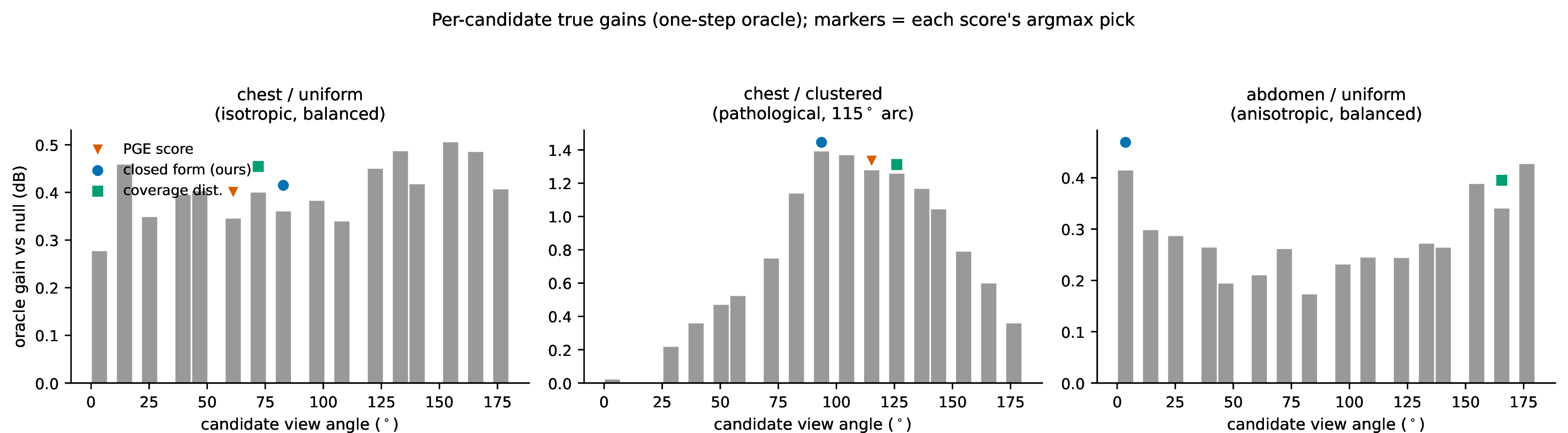
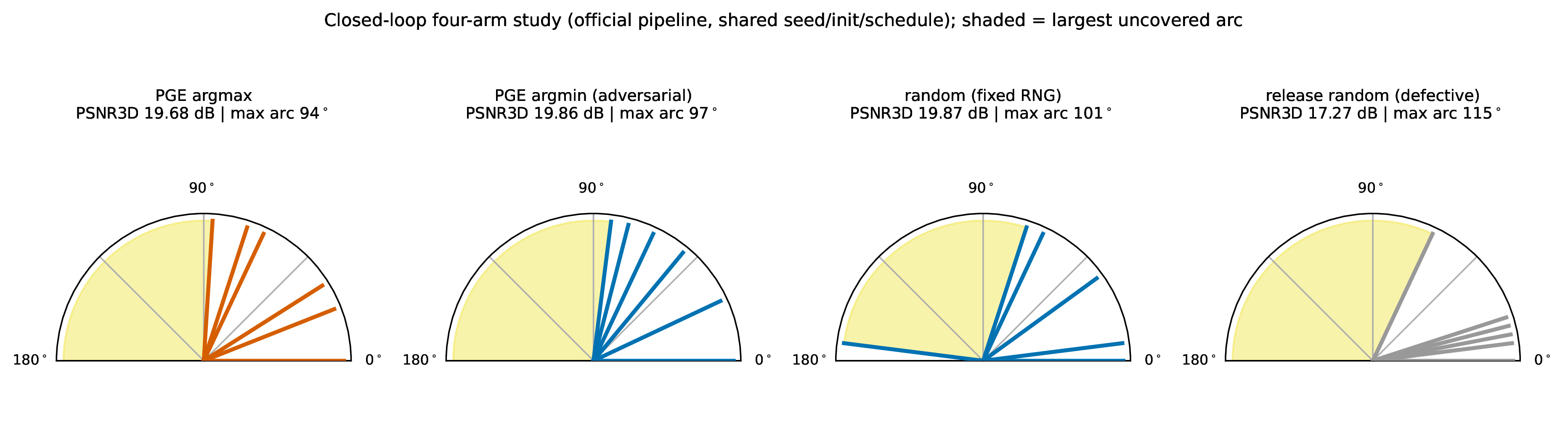
We dissect the concurrent perturbation-ensemble acquisition score with four complementary probes on our circular-orbit testbed (Fig. 4–5).
4.7.0.1 Four-arm closed loop.
Using the official closed-loop trainer, argmax, argmin, and fair random selection differ by only 0.19 dB PSNR (19.68/19.86/19.87 dB); the sole large failure is degenerate angular clustering (\(-\)2.6 dB, 115\(^\circ\) max gap). We report this as indistinguishable within expected seed noise; a matched multi-seed noise floor for the same configuration was not measured (Limitations).
4.7.0.2 View-level oracle.
One-step oracle gains vary by regime: nearly flat on uniform chest (\(+0.28\)–\(0.51\) dB spread — selection is low-stakes), wide on pathological clustering (\(+0.02\)–\(1.39\) dB, where every signal including free geometry lights up: score–gain Spearman \(+0.92\) competitor, \(+0.70\) ours, \(+0.81\) coverage distance), and structured on anisotropic abdomen (\(+0.17\)–\(0.43\) dB). The abdomen regime is the one where an uncertainty signal earns its keep: coverage distance cannot see the directional structure (score–gain Spearman \(+0.25\), \(p{=}0.36\)) while both uncertainty scores can (\(+0.84\), \(p{<}10^{-4}\) competitor; \(+0.62\), \(p{=}0.01\) ours; \(n{=}16\)).
4.7.0.3 Schedule autopsy.
In the official loop the first scored pick occurs at iteration 1500 with only \(\sim\!10^2\) Gaussians; score–coverage Spearman is \(-0.13\) and remains \(\le 0\) thereafter, while the same score computed offline on a converged model facing a comparable large uncovered arc aligns strongly (score–coverage Spearman \(+0.86\)).
4.7.0.4 Symmetric self-test.
On uniform chest, neither our closed-form score nor the competitor’s shows a detectable positive rank correlation with true oracle gains (point estimates \(-0.32\) and \(-0.41\), \(n{=}16\), neither significant): both scores fail symmetrically where no directional signal exists.
4.8 What SSIM aggregation actually contributes↩︎
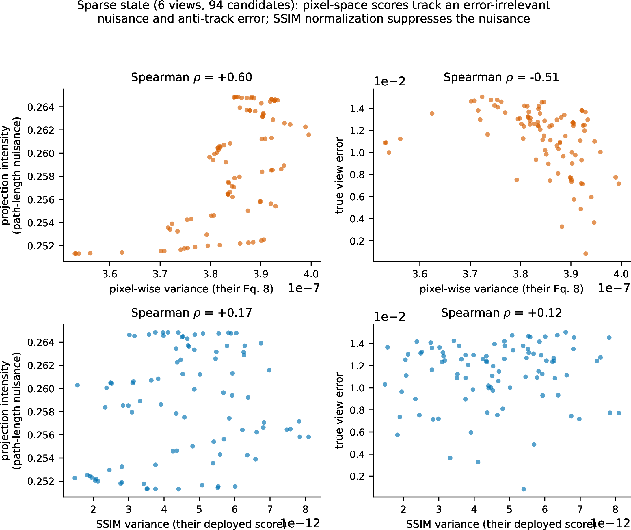
Fig. 6 compares pixel-space variance (their Eq. 8) against SSIM-based variance on 94 sparse-view candidates. Pixel variance correlates with projection intensity (\(\rho{=}+0.60\)) — an error-irrelevant nuisance, since intensity itself correlates with true error at only \(-0.13\) — and anti-correlates with true view error (\(\rho{=}-0.51\)); SSIM normalization reduces the nuisance loading to \(+0.17\) and is the only statistic whose error correlation is not negative, though it is not distinguishable from zero either (\(+0.12\), \(n{=}94\), \(p{=}0.27\)). On a denser 25-view chest state the ranking reverses (pixel variance vs.error \(+0.53\) exceeds SSIM \(+0.26\)), so SSIM aggregation is a state-dependent nuisance suppressor rather than a universal fix. We state this as a mechanistically consistent account of a signal-level measurement, one inferential step removed from the concurrent work’s end-to-end ablation, not a refutation of it.
5 Coverage-gated acquisition on the testbed↩︎
We evaluate CGCA (Sec. 3.5) on our circular-orbit testbed: 50 candidate angles on a \(180^\circ\) half-scan (\(3.6^\circ\) spacing), shared 2-view initialization (candidate indices 0 and 18, i.e.\(0^\circ\) and \(64.8^\circ\), leaving a \(115.2^\circ\) initial gap), and budget \(B{=}12\). Mechanism experiments (Sec. [sec:experiments-mechanism]) motivate the design: degenerate clustering is the dominant failure mode (\(-\)2.6 dB), scores queried on immature models are noise, and closed-form variance earns a premium only in anisotropic regimes.
5.0.0.1 Protocol (select-then-train).
Each policy sequentially selects a view set \(\mathcal{A}\) with \(|\mathcal{A}|{=}B\). Selection uses either geometric gap-filling (coverage gate, threshold \(\gamma{=}30^\circ\)) or, once \(\mathrm{gap}(\mathcal{A})\le\gamma\), scores from a variational model retrained to convergence on \(\mathcal{A}\) (10k iterations). After selection, every arm retrains a final model with identical commands and hyperparameters (\(n{=}3\) seeds), so reported PSNR differences are attributable strictly to view-set quality.
5.0.0.2 Six-arm comparison.
Table 6 compares six policies on abdomen (anisotropic) and chest (isotropic): uniform, random, geo (coverage gate only), pge (our CGCA shell — the coverage gate plus
maturity schedule of Sec. 3.5 — carrying the competitor’s SSIM-variance score), full_raw (shell + raw closed-form \(\sum_p\mathrm{Var}[I_p]\)), and full
(shell + D-optimal log form, ablated after pre-registration).
| Scene | Policy | PSNR3D | Final max gap |
|---|---|---|---|
| Abdomen | Uniform | 26.67\(\pm\)0.03 | 18.0\(^\circ\) |
| Chest | Uniform | 25.41\(\pm\)0.02 | 18.0\(^\circ\) |
| Abdomen | Random | 25.61\(\pm\)0.01 | 57.6\(^\circ\) |
| Chest | Random | 24.31\(\pm\)0.02 | 57.6\(^\circ\) |
| Abdomen | Geo gate only | 26.43\(\pm\)0.00 | 18.0\(^\circ\) |
| Chest | Geo gate only | 25.39\(\pm\)0.02 | 18.0\(^\circ\) |
| Abdomen | Shell + PGE score | 27.35\(\pm\)0.05 | 28.8\(^\circ\) |
| Chest | Shell + PGE score | 25.17\(\pm\)0.02 | 28.8\(^\circ\) |
| Abdomen | Shell + raw closed-form | 27.29\(\pm\)0.02 | 28.8\(^\circ\) |
| Chest | Shell + raw closed-form | 25.17\(\pm\)0.01 | 28.8\(^\circ\) |
| Abdomen | Shell + log closed-form | 25.94\(\pm\)0.03 | 28.8\(^\circ\) |
| Chest | Shell + log closed-form | 24.59\(\pm\)0.01 | 28.8\(^\circ\) |
5.0.0.3 Findings.
On abdomen, the coverage shell is decisive: random collapses to 25.61 dB while geo recovers 26.43 dB (+0.82 dB). With the shell engaged, pge reaches 27.35 dB (+0.68 dB over uniform) and full_raw lands
within \(0.07\) dB at 27.29 dB (\(\pm\)0.02); the gap is \(\approx\!2\times\) the pooled standard error, which at \(n{=}3\)
seeds falls short of significance, so we do not claim an ordering in either direction. The ablated log score (full) loses 1.35 dB on abdomen because saturated \(\log(1+\mathrm{Var}/\sigma_n^2)\) ranks by
variance footprint size.
5.0.0.4 Isotropic cost.
On chest, geo matches uniform (25.39 vs. dB); enabling phase-2 scoring (pge, full_raw) costs \(\approx\)0.24 dB relative to uniform while leaving a larger final angular gap
(28.8\(^\circ\) vs.\(^\circ\)).
5.0.0.5 Scope.
CGCA is validated only on the circular-orbit testbed; hemispherical pose pools require a spherical coverage metric and a replication under the concurrent work’s native protocol, both left to future work.
6 Discussion↩︎
6.0.0.1 Calibration and acquisition decouple.
Uncertainty for 3DGS-CT has so far been validated through the reconstruction quality of the views it selects. Our results argue that this substitution is unsound, because acquisition is a structurally forgiving consumer of an uncertainty signal, in three distinct ways. First, it consumes only the argmax of a ranking: a decision worth a few bits per round, invariant to any monotone distortion of the score, and blind by construction to whether the predicted magnitudes are right at all. Second, it operates inside a closed loop — a mediocre pick still returns information, and retraining absorbs the loss. Third, in the balanced isotropic states we tested there is simply nothing to win: true one-step gains span \(0.23\) dB at the resolution of our oracle, so every candidate is nearly as good as the best one. Consistently, using the concurrent score forwards, backwards, or not at all is indistinguishable in a closed loop (4.7). Per-voxel interpretation is forgiving in none of these ways: it consumes millions of magnitudes rather than one argmax, a clinician reading \(\sigma(x)\) has no feedback loop that could correct a wrong map, and a signal that fails to track error — the perturbation heuristic’s rank correlation dips below zero on head (\(-0.08\)) — offers no reliable localization exactly where trust matters. Uncertainty should therefore be validated where it is consumed — against error, with rank and coverage metrics — and acquisition should be treated as a downstream application that principled uncertainty serves in specific, identifiable regimes (anisotropic content; plus the prospect of a calibrated stopping rule, which no ranking heuristic can even express and which we leave to future validation).
6.0.0.2 Limits of mean-field marginals.
The flat-regime null result for our own score localizes a real limitation: the acquisition-relevant quantity is \(\log\det\) of a posterior block, and factorized marginals discard the along-ray negative correlations that make acquired directions certain. That gross imbalance and anisotropic structure remain visible to marginal variances — while fine ranking in balanced states does not — is, to our knowledge, the first empirical delineation of where mean-field uncertainty suffices for view planning. Correlation-aware extensions (low-rank plus diagonal posteriors) are a natural next step.
7 Limitations↩︎
All evaluations use synthetic benchmarks with exact ground-truth volumes. This is a deliberate methodological choice — voxel-wise calibration assessment requires a ground truth that real cone-beam scans cannot supply exactly, since their reference volumes are themselves reconstructions — but transfer of both reconstruction and calibration behavior to measured clinical data remains untested. The mechanism study ([sec:why-uncalibrated] [sec:ssim]) uses one development scene per regime, single seeds, and a one-step 1k-iteration frozen-topology oracle; the oracle’s short horizon may compress gain spectra, and the closed-loop arms lack a measured same-configuration noise floor, so we report indistinguishability rather than ordering. All reproduction results use the official code release on our data (theirs is unreleased at the time of writing); we found and patched two defects in the release (an unmaintained data path and a per-round RNG re-seeding bug that degenerates the random baseline into consecutive views) and cannot determine whether published numbers were affected — published multi-scene averages are in any case measured under a hemispherical protocol we have not yet replicated at scale. Amplitude calibration after a single global temperature does not fully generalize to the official benchmark: four scenes sit marginally above our scaled-ECE target of \(0.1\) (\(0.103\)–\(0.112\)), and on near-noise-floor objects (beetle, and partially teapot) the error distribution collapses toward zero so that no single scalar can align a Gaussian predictive to it — rank metrics remain strong on exactly these scenes (Spearman \(0.85\)–\(0.91\), AUSE \(0.02\)–\(0.07\)), so the residual is a shape mismatch of the predictive distribution, not a localization failure; per-scene shape-aware recalibration is future work. Within the \(0.09\)–\(0.12\) scaled-ECE band the metric itself is fragile: ordinary CUDA training nondeterminism perturbs the learned \(\sigma\) field by a few percent, which the \(\tau\)-argmin and binned-ECE pipeline amplifies, flipping the pass/fail identity of three marginal scenes between two GPUs while the gate count stays \(\ge 8/15\) in four of five completed machine\(\times\)grid combinations (4.3); on one scene the fitted temperature is bistable across seeds (7). We report per-seed temperatures and treat marginal-band membership as machine-dependent. One benchmark scene (jaw) has a near-flat error field (an error floor) on which no spatial ordering can score well; we report it and exclude no scene from any average. The variational posterior is partial (density only) and factorized; its projection variance is blind to fine-grained view ranking in balanced isotropic states (4.7). Temperature scaling is fitted per scene with a within-scene fit/evaluation voxel split (3.4) — an earlier version of our tooling fitted and reported \(\tau\) on the same sample; we re-derived all quoted scaled-ECE numbers under the split protocol, which changed them by \(\le 0.001\) — and \(\tau\) transfer across scenes and scanner geometries remains to be tested. Our evaluated MC uncertainty clamps sampled densities at zero to match training; it therefore estimates the truncated predictive distribution rather than the exact linear-model variance the closed form computes (3.3), and the two differ systematically in high-uncertainty regions (on the official benchmark the MC estimator scores better on both rank and scaled ECE in all 75 runs, 8.2). The dose-adaptive stopping rule enabled by the calibrated posterior (3.5) is stated as a design implication only; no stopping experiment is reported in this paper. The clustered-state oracle shares its FDK-based initialization with the uniform-state arm — a mild information leak into the uncovered arc, common to both arms; the schedule autopsy is a single instrumented run, and we observed same-seed early-training divergence in the official pipeline (one run collapsed entirely, one survived), so per-round statistics should be read as illustrative.
8 Additional results and protocol details↩︎
8.1 Temperature bistability and grid truncation↩︎
7 documents two temperature-fitting phenomena behind the boundary-band fragility discussed in 4.3 and 7: (i) on foot, the fitted \(\tau\) alternates between two basins (\(\approx 9\) vs.\(\approx 21\)) across seeds under an identical protocol, moving scaled ECE between \(0.06\) and \(0.11\); (ii) on kingsnake and teapot, our original legacy grid (\([0.1,30]{\times}60\)) silently truncated the fit at \(\tau{=}30\), inflating the 3-seed mean scaled ECE on kingsnake from \(0.103\) (wide grid) to \(0.177\). Because fitted temperatures reach \(\tau \approx 90\)–\(110\) for the MC maps and, on one run (beetle, 75-view), \(\approx 750\) for the closed form — whose next-largest fit is \(50.8\) — we recommend that any temperature-scaled ECE protocol log the fitted \(\tau\) and assert that it does not touch the grid boundary; our tooling flags boundary hits automatically, and no reported fit touches the wide-104 bound (the intermediate wide-80 grid still truncated two runs, which is why the final protocol widens to \(1000\)).
| Run | \(\tau\) (wide) | scaled ECE (wide) | \(\tau\) (legacy) | scaled ECE (legacy) |
|---|---|---|---|---|
| chest, seed 0 | 6.7 | 0.0994 | 6.4 | 0.0998 |
| chest, seed 1 | 6.7 | 0.1005 | 6.4 | 0.1008 |
| chest, seed 2 | 6.1 | 0.0959 | 6.4 | 0.0954 |
| foot, seed 0 | 21.4 | 0.0602 | 22.4 | 0.0570 |
| foot, seed 1 | 9.0 | 0.1124 | 8.5 | 0.1128 |
| foot, seed 2 | 9.0 | 0.0863 | 9.4 | 0.0840 |
| kingsnake, seed 0 | 50.8 | 0.1062 | 27.2 | 0.1433 |
| kingsnake, seed 1 | 74.6 | 0.1048 | 30.0 | 0.1975 |
| kingsnake, seed 2 | 90.4 | 0.0970 | 30.0 | 0.1895 |
| teapot, seed 0 | 90.4 | 0.1221 | 30.0 | 0.1511 |
| teapot, seed 1 | 55.9 | 0.0835 | 30.0 | 0.1358 |
| teapot, seed 2 | 90.4 | 0.1264 | 30.0 | 0.1407 |
8.2 MC vs.closed form on the official benchmark↩︎
On all 75 official-benchmark runs, the clamped-MC estimator (B1, \(S{=}16\); 3.3) scores better than the single-pass closed form (B2) on both Spearman (75/75) and temperature-scaled ECE (75/75), consistent with B1 tracking the truncated predictive distribution used at training time. B2’s volume-domain Pearson agreement with \(S{=}8\) clamped-MC reference maps on these runs is \(0.76\)–\(0.84\) (versus \(0.80\)–\(0.88\) against the references of 4 on the development scenes). Headline calibration tables therefore use B1; B2 remains the single-pass deployment path for acquisition scoring (3.5) and efficiency-critical use.
8.3 Cross-machine reproducibility↩︎
An independent replication of the benchmark on a second consumer GPU (RTX 5080 laptop) reproduces PSNR3D and Spearman closely (scene-mean differences within \(\pm 0.05\) dB and \(\pm 0.02\)), and scaled ECE on most scenes to the third decimal (e.g.pancreas \(0.108\) and mount \(0.111\)–\(0.112\) on both machines). The exception is the \(0.09\)–\(0.12\) scaled-ECE boundary band, where seven scenes sit at the 25-view tier: there, few-percent differences in the learned \(\sigma\) field — ordinary CUDA training nondeterminism — are amplified by the \(\tau\)-argmin and binned-ECE pipeline, and three boundary scenes (chest, foot, kingsnake) flip pass/fail between machines. The gate count is stable even when the identity of the marginal scenes is not: legacy grid, \(9/15\) (RTX 4060) vs.\(7/15\) (RTX 5080); wide-80 grid, \(9/15\) vs.\(8/15\); wide-104 grid, \(9/15\) (RTX 4060; the second machine’s wide-104 recompute was pending at the time of writing). We therefore read the marginal band as genuinely marginal and report per-seed temperatures (7) rather than presenting any single draw as definitive.
8.4 Reproduced defects in the concurrent release↩︎
For completeness we record two defects found and patched in the official release of the concurrent method during our reproduction (7): (i) a data-reader path that omitted the lon/lat fields on
non-Blender inputs, and (ii) a per-round RNG re-seeding that collapses the “random” baseline into consecutive views. We report these as reproduction observations; we cannot determine whether published numbers were affected, and all our random baselines use
a fixed-RNG reimplementation.