STOCKTAKE: Measuring the Gap Between Perception and Action in LLM Agents with a Fair Oracle
July 15, 2026
Abstract
LLM agents are increasingly evaluated on multi-week decision tasks in which the state that drives cost is never directly observed. On such tasks the final cost cannot say why an agent failed. It may have misread the world, or it may have read the world correctly and still failed to act (the knowing-doing gap). Existing evaluations cannot separate these two failures: their reference policies either read privileged information the agent never sees, or are missing altogether. We introduce STOCKTAKE, a 26-week supply-chain replenishment benchmark built as a factored partially observable Markov decision process (POMDP) with six hidden factor processes, designed so that a fair reference policy is computable: an exact Bayes filter per factor drives a rollout policy on the identical observation stream the agent receives. Scoring each run between a symptom-blind base-stock floor (0) and this oracle (1) yields a skill score, and grading each week’s written rationale yields a stated-belief detection lag and a knowing-doing rate, so state estimation and control are measured separately. On fifty seeds with curated stress profiles, Claude Sonnet 5, GPT-5.4, DeepSeek-V4-Pro, and Grok 4.5 detect 84–88% of hidden failures, typically within a week of onset, yet span skill scores from \(0.62\) to \(-0.23\): two of the four end below the symptom-blind floor while naming factors slightly faster than the two that beat it. The failure has two faces. Where stress persists, 34–43% of correctly diagnosed stress weeks still end in stockout for every model (a rate that partly reflects the severity of the weeks models notice; Section 5). That rate also runs opposite to skill: the two models under the floor stock out least on diagnosed weeks, so under-response is only one face of the gap, and their traces point to the other — responses whose cost exceeds what they protect. The bottleneck for current agents sits between a correct stated belief and the costly action it calls for; STOCKTAKE measures both directions of that failure.
1 Introduction↩︎
LLM agents are increasingly evaluated on long-horizon decision tasks: running a vending machine for months [1], managing a retail store [2], operating supply chains [3], [4]. These tasks share a structure. The world has hidden state, such as a demand shift or a failing supplier, that the agent can only infer from noisy symptoms, and performance depends on acting on those inferences week after week. Benchmarks in this genre consistently report that agent performance degrades over long horizons. What they largely cannot report is why.
When an agent incurs excess cost on such a task, two distinct failure modes are possible. It may have failed to infer the hidden state, never recognizing that demand had shifted; or it may have inferred correctly and failed to act, stating the correct diagnosis in its reasoning while placing the wrong order. The second failure mode is documented in bandit and game settings under the name of the knowing-doing gap [5], [6]: models often hold or state correct beliefs about the task yet fail to act on them. These are failures of perception and failures of action — in the language of partially observable decision processes, failures of state estimation and failures of control — and they call for different fixes: better inference scaffolding in the first case, better policy elicitation in the second. Telling them apart, however, requires knowing what a correct inference was worth.
Existing evidence for the knowing-doing gap does not support that accounting. It comes from probes and single decisions in settings where the correct action is known in closed form [5], [6], or from cost comparisons against a reference policy that sees privileged information: the oracle in RetailBench, for instance, is computed with access to ground truth the agent never observes [2]. A privileged oracle conflates the two failure modes by construction, because the shortfall it measures bundles “did not know” and “knew but did not act” into one number. To attribute cost to the knowing-doing gap specifically, the reference policy must be denied exactly the information the agent is denied.
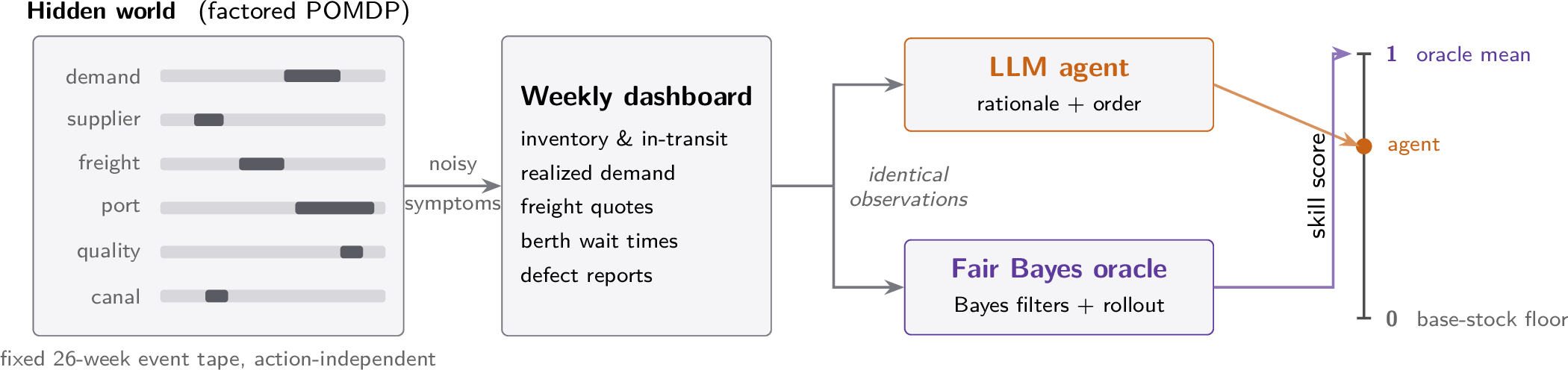
We introduce a benchmark in which that fair reference is computable. The task is a 26-week inventory-replenishment problem, formalized as a factored POMDP with six hidden factor processes whose states the agent must infer from noisy weekly symptoms (Section 3). Because the hidden structure is factored and the event tape fixed, an explicit Bayesian reference policy is feasible: an exact Bayes filter per factor driving a rollout policy, conditioned on exactly the observation stream the LLM receives. This reference is fair rather than privileged; Section 4 states the one disclosed asymmetry. Together with a symptom-blind base-stock floor, it yields a skill score locating each agent between ignoring the symptoms (0) and matching the fair Bayesian (1), and two rationale-based metrics, detection lag and the knowing-doing rate, that separate state estimation from control. Fifty seeds, grouped by stress profile (isolated, persistent, compound), make the interaction of hidden failures a controlled variable.
Our contributions are:
We introduce a six-factor supply-chain POMDP benchmark whose upper reference is a fair, computable Bayes-filter oracle: an exact-filter rollout policy conditioned on the identical observation stream as the agent, referenced as the mean of 20 replications per seed. Fairness is what makes agent shortfall attributable to acting rather than confounded with knowing.
We construct a controlled stress axis (isolated / persistent / compound) that varies whether and how hidden failures overlap while holding the world model fixed.
We measure state estimation and control separately — skill score, detection lag, knowing-doing rate — over 200 episodes: Claude Sonnet 5, GPT-5.4, DeepSeek-V4-Pro, and Grok 4.5, each on all fifty seeds, under a rules-only prompt with no strategy playbook.
Across 200 episodes, detection proves nearly uniform: all four models name 84–88% of hidden-factor episodes, typically within a week of onset, and the two models with the lowest skill scores name them fastest. Costs diverge sharply nonetheless: two of the four models finish below the symptom-blind floor overall — on roughly half their seeds, a rule that reads no symptoms at all would have been cheaper than acting on their largely correct diagnoses. The gap also concentrates: on persistent seeds, 34–43% of correctly diagnosed stress weeks still end in stockout for every model, a rate Section 5 shows is partly severity (weeks bad enough to notice are also bad enough to strain the shelf). What separates models is the distance between seeing a problem and acting on it, and the failures run in both directions: ordering too little too late, and paying too much for protection.
2 Related Work↩︎
5pt
Evaluating LLM agents as sequential decision-makers has grown from single-turn tool use into month-scale simulations of running a business. Vending-Bench [1] has agents operate a vending machine across two thousand messages and finds coherence collapse, ruling out context exhaustion as the cause. RetailBench [2] simulates a supermarket built on real retail records, frames it as a partially observable decision process, and finds that only a few models survive its 180-day horizon. In inventory management specifically, AIM-Bench [3] finds human-like ordering biases (demand anchoring, bullwhip amplification) across five environments, and InvAgent [4] reports outcome gaps against heuristic and reinforcement-learning baselines in a fully observed twelve-period setting.
A second line of work asks whether agents act on what they know. In bandit tasks, models produce a correct rationale for 87% of decisions and still take the greedy action over the optimal action they just derived [5]. Probing studies in strategic games find internal beliefs about the opponent that are often accurate, weakly verbalized, and weakly linked to the chosen action [6]. Probes of tool-use decisions find the same split inside the network: the belief that an action is needed and the action taken are both linearly decodable, but their directions drift apart in later layers [7]. The phenomenon has a name, the knowing-doing gap, and it has so far been measured on decisions whose correct answer is known in closed form.
A third line evaluates the beliefs themselves. BayesBench [8] scores posterior updating against a rational Bayesian reasoner and finds systematic departures, on estimation tasks with no actions attached. The machinery for connecting such beliefs to inventory decisions is classical: Bayraktar and Ludkovski [9] derive the exact Bayes-filter reduction of inventory control with hidden Markov-modulated demand to a fully observed problem, in their case to compute optimal policies.
The task is causal only in a specific, limited sense, and we place it against that literature explicitly. Causal-reasoning benchmarks test whether a model can recover causal structure or answer interventional and counterfactual queries [10], and there is evidence that models recite causal facts from text rather than infer them [11]. Our task tests neither: the causal structure of the world is given to the agent in the prompt, and actions never touch the hidden dynamics, so there is nothing to discover and nothing to intervene on. What the weekly decision demands is abduction, inferring which hidden cause best explains the week’s noisy symptoms under a known model, followed by cost-sensitive control. The benchmark is complementary to causal-reasoning evaluations: it measures whether a correct causal attribution, once formed, survives the trip to an action.
Table 1 summarizes the benchmarks closest to ours. In each, the reference policy either reads information the agent is denied (RetailBench’s rule-based oracle takes “structured simulator fields” as input; AIM-Bench’s ex-post optimum is computed from realized demand) or is absent beyond a single human run, and none grades the agent’s stated beliefs alongside its actions. STOCKTAKE addresses both limitations with one construction: the classical filter reduction, repurposed as a reference policy conditioned on exactly the agent’s observation stream, so that shortfall against it isolates the action side of the knowing-doing gap, while the weekly stated beliefs it is compared against are graded on the same episodes.
3 STOCKTAKE: Task and Environment↩︎
STOCKTAKE casts the agent as the replenishment manager of an electronics importer for a 26-week episode. The state that drives cost is never observed directly. The agent reads weekly symptoms, commits an order, and writes down what it believes is happening (Figure 1).
3.1 The weekly decision↩︎
Each week the agent reads a dashboard of on-hand inventory, orders in transit, realized demand, freight quotes, berth waiting times, canal transit counts, supplier scorecards, and quality reports. It may then take any of five within-week actions, none
of which advances time. lock_freight fixes the current freight multiplier for a chosen number of weeks; the lock itself is free, but a locked rate forgoes any drop in the spot index. expedite_air flies up to 20 units in at $15 per
unit; they land the following week and bypass the port entirely. inspect_batch ($40) sorts an arriving batch so that most defective units are recovered before they stock. buy_briefing ($30) and buy_audit ($25) reveal
the true state of the canal and of the spot supplier, respectively.
The week is then committed by exactly one call to place_order(rationale, qty, route, supplier, contract). The order names a quantity, a route (through the Suez Canal, or slower and dearer around the Cape), and a supplier; the optional
contract action signs, switches, renews, or lapses a supplier contract on short, long, strict, or lenient terms, and the agent can only source suppliers it holds a live contract with. The rationale argument is required, and the world does not
advance without it. Every run therefore contains 26 written statements of what the agent believed each week; Section 4 derives the belief-side metrics from them.
Costs accrue for units held and in transit, for demand missed, and for the priced levers above; the episode score is total cost, lower is better. The price ladder is the task’s core tension: sea freight is $4 per unit and takes three weeks, air is $15, and every unit of missed demand costs $20. An agent that reads the symptoms early can buy its way out of trouble cheaply; one that reads them late cannot.
3.2 The hidden world↩︎
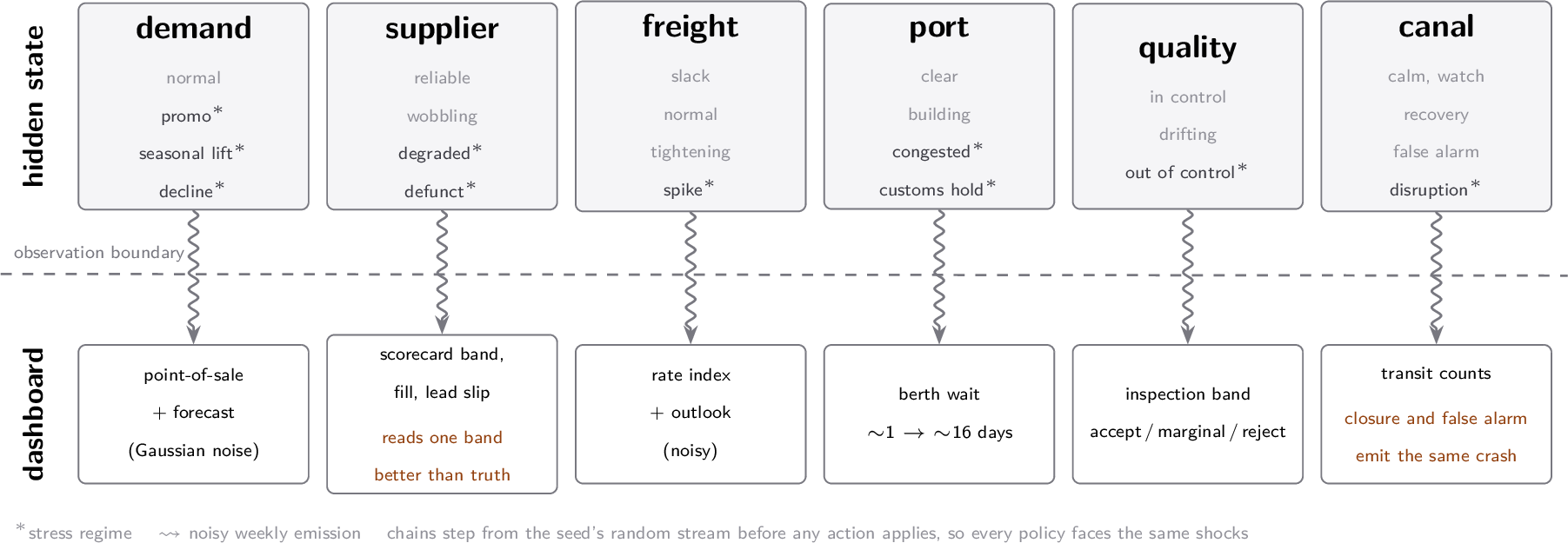
The environment is a factored POMDP. Two structural properties of its hidden state make a fair reference policy computable. Let \(x_t = (x_t^1, \dots, x_t^6)\) denote the hidden state in week \(t\), one factor process each for demand regime, supplier health, freight market, port congestion, batch quality, and canal status, each a small Markov chain over regime–age pairs that moves between a baseline and one or more stress regimes (Figure 2). The regime and its age set the transition probabilities: how likely a stress episode is to start, to persist once started, and to resolve.
First, the dynamics are factored and action-independent. Each factor steps as \(x_{t+1}^i \sim P^i(\cdot \mid x_t^i)\), reading neither the other factors nor the agent’s action. Algorithm 3 is the entire generative process: one random stream, seeded once, consumed by the six factors in a fixed order. Because no step reads an action, the seed fixes every regime change and every noisy reading for all 26 weeks before the agent exists; we call this fixed record the episode’s event tape. Two policies run on the same seed face byte-identical shocks and symptom noise, so the reference policies of Section 4 are evaluated on the very tape the agent lived through, not on a re-rolled one. Actions decide how much each shock costs, never what happens in the hidden world.

The port factor instantiates the template. From clear, the port can start building toward a backlog or take a sudden customs hold (line 6); building tips into congested or clears (line 8); congested persists week to week until its age cap forces recovery. Each week the realized berth wait is drawn around the current band’s mean, roughly one day when clear and sixteen when congested, and while congested every arriving shipment is held an extra week. The band on line 11 is where the benchmark’s ambiguities are constructed: for several factors the first week of two different regimes maps to the same band, so a fresh customs hold and newly tipped congestion both read “slow”, and a demand promotion and a seasonal lift both open on the same “surge”. A single reading cannot say which stress has begun; only the following weeks separate them. A few factors draw auxiliary state from the same stream in the same fixed order, such as the canal event’s type at onset.
Second, the observations are factored. The weekly dashboard \(o_t\) contains the fully observed logistics state (on-hand stock, orders in transit, realized demand) and one symptom channel per factor, \(y_t^i \sim Q^i(\cdot \mid x_t^i)\). The agent never observes any \(x_t^i\) directly; the paid briefing and audit of Section 3.1 are the only exceptions, each revealing one factor’s current state for a fee. The channels themselves are hard to read in three different ways. Most are noisy: a building port and a clear one differ by a few days of berth wait, against scatter of the same size. The supplier scorecard is biased, reading one severity band better than the truth by design. The canal channel is exact but ambiguous, emitting the same transit-count crash for a false alarm as for the first week of a real closure, so even a Bayesian observer should be uncertain there.
The cost function, by contrast, is not factored. The factors evolve independently but bill jointly through a single set of books: a port hold delays the same shipments a demand surge is waiting on, and a quality escape shrinks the same inventory that surge is draining. Concurrent shocks can therefore cost far more than the same shocks arriving in sequence, and Section 3.3 samples that regime deliberately. Full cost constants, caps, lead times, and per-factor transition parameters are in Appendix 7.
3.3 Seeds and stress profiles↩︎
Because the tape is a pure function of the seed (Algorithm 3), instances can be minted and classified before any agent exists. Any unsigned integer names a candidate: the world is replayed to week 26 with empty actions, and the resulting tape is summarized by a handful of features — the number of stressed weeks per factor, how many weeks have two or more factors stressed at once and the most stressed simultaneously, the longest unbroken run of port blockage, and whether the spot supplier failed outright. Thresholds on these features classify the candidate’s stress profile, and candidates too benign to separate good decision-making from bad (those on which the two reference policies of Section 4 cost nearly the same) are discarded. The benchmark fixes fifty seeds chosen this way from a 200-seed pool:
isolated (12 seeds), short, non-overlapping single-factor shocks;
persistent (15 seeds), a multi-week stretch of port congestion overlapping a demand rise. Here the intuitively appealing response, freezing orders until the congestion clears, is the costly one, because orders placed through the congestion arrive as it clears;
compound (23 seeds), pileups of three or more concurrent factor episodes.
Compound stress is deliberately oversampled relative to the pool; it is the regime the benchmark targets, and all results are reported per group. Because membership is fixed by the tape alone, the structure of hidden stress is an independent variable of the benchmark, and the same minting recipe extends it: new instances of any profile can be generated and classified with no agent runs and no human labeling.
3.4 Agent prompt↩︎
Agents run under a single rules-only prompt that specifies the mechanics of the task (costs, lead times, levers, output format) and gives a qualitative description of the world’s factors, with no strategy advice, no playbook, and no worked examples. The benchmark thereby measures what a capable agent brings to the task on its own. The full prompt and the weekly observation format are reproduced in Appendix 11.
4 Experimental Setup↩︎
Reference policies. Every run is scored between two reference policies evaluated on the same seed, and both are functions of the agent’s own observation stream \(o_{1:t}\), nothing more. The floor is a textbook base-stock policy: order up to a fixed target \(S = \mu L + z\sigma\sqrt{L}\) (mean demand \(\mu\), lead time \(L\), safety factor \(z\) from the holding/stockout cost ratio) every week, always by the same route and supplier, reading no symptom channel \(y_t^i\) at all. The upper reference is the Bayes-filter oracle of Figure 1. Because the dynamics and the observations both factor and neither reads the action (Section 3.2), the posterior over the hidden state splits into six independent parts, each small enough to maintain exactly: one forward (predict–correct) filter per factor tracks \(b_t^i = \Pr(x_t^i \mid y_{1:t}^i)\), updated each week on the same observation dictionary \(o_t\) that is serialized into the LLM prompt. To act, the oracle samples \(\sim\)200 possible futures of all six factors from the belief \(b_t = (b_t^1, \dots, b_t^6)\), scores a small menu of candidate actions (order sizes, routes, each mitigation lever, gated on the relevant posterior risk) against every sampled future, and executes the cheapest candidate through the same action API the LLM uses. Its randomness is independent of the world’s, and it never reads hidden state. One asymmetry is disclosed: its filters use the environment’s true generative parameters (the transition tables \(P^i\) and the regime means behind \(Q^i\)), which the LLM receives only as a qualitative description. We therefore interpret the oracle as Bayes-optimal given the true model. Because it is a stochastic policy, its per-seed reference value is the mean of 20 replications (standard error 0.2–1.8% of the reference cost); it is a fair reference rather than an optimum, and agents exceed it on some tapes (Section 5). Appendix 8 specifies both policies in full.
Metrics. Let \(C_{\mathrm{base}}\), \(C_{\mathrm{orc}}\), and \(C_{\mathrm{agent}}\) denote total episode cost for the floor, the oracle reference, and the agent. The skill score \[\mathrm{skill} \;=\; \frac{C_{\mathrm{base}} - C_{\mathrm{agent}}}{C_{\mathrm{base}} - C_{\mathrm{orc}}}\] is 0 at the symptom-blind floor and 1 at the oracle mean; values above 1 and below 0 both occur. One of the fifty seeds has negative headroom (\(C_{\mathrm{base}} < C_{\mathrm{orc}}\)): the floor already beats the oracle mean on that tape, so skill is undefined there, and the seed is excluded from every skill mean (leaving \(n = 49\)). Its runs still count in a denominator-free companion statistic, the number of seeds on which the agent’s raw cost beats the floor’s. Three further seeds have headroom under $700, where the ratio is noisy; they are flagged in the per-seed results but not excluded. A worked example from seed 1: base-stock costs $9,101, the oracle mean is $6,932, and Claude Sonnet 5 spent $8,539, so its skill is \((9101-8539)/(9101-6932)=0.26\) — it recovered about a quarter of what seeing the symptoms was worth on that tape. For belief-side metrics, a stress episode is a maximal run of consecutive weeks in which one factor is truly in a stress regime (283 episodes per model across the fifty tapes). Detection lag is the number of weeks from episode onset until the factor is first named in the agent’s rationale (averaged over detected episodes; never-detected episodes are reported separately), and the knowing-doing rate is \[\mathrm{KD} \;=\; \Pr\!\left(\,\text{stockout in week } t \;\middle|\; \text{a truly stressed factor is named in week } t\,\right),\] estimated over the group’s correctly diagnosed stress weeks, where “stockout” means the stock available that week (inventory plus arrivals) fell short of realized demand. A high KD rate means correct diagnosis coexisting with empty shelves.
Belief grading. Whether a rationale names a factor is judged by a small LLM grader (gpt-5-mini, temperature 0) that sees only the rationale text and the fixed factor vocabulary, never the tape; labels are aligned to the week the rationale was written. Grader labels were audited in two rounds against raw traces; residual disagreements are borderline over-labels on calm weeks, which cannot enter the knowing-doing rate by construction. The rationale is stated belief: a lower bound on what the model knows, a point we return to in Section 6. Grading rules and validation details are in Appendix 9.
Models. We evaluate Claude Sonnet 5, GPT-5.4, DeepSeek-V4-Pro, and Grok 4.5, each on all fifty seeds. All four run through an identical harness (OpenRouter model IDs anthropic/claude-sonnet-5, openai/gpt-5.4,
deepseek/deepseek-v4-pro, x-ai/grok-4.5; temperature 0; runs completed July 2026), one run per model–seed pair, 200 episodes in total, each validated to the full 26 weeks, all under the rules-only prompt of Section 3.1
5 Results↩︎
| Model | isolated | persistent | compound | All | neg | beats floor |
|---|---|---|---|---|---|---|
| Claude Sonnet 5 | 0.54 (0.71) | 0.70 (0.61) | 0.33 (0.35) | 0.49 (0.45) | 9 | 40/50 |
| GPT-5.4 | 0.21 (0.07) | 0.55 (0.61) | 0.86 (0.73) | 0.62 (0.65) | 8 | 42/50 |
| DeepSeek-V4-Pro | \(-\)0.62 (\(-\)0.57) | \(-\)0.68 (\(-\)0.26) | 0.24 (0.32) | \(-\)0.23 (0.15) | 22 | 28/50 |
| Grok 4.5 | \(-\)0.14 (\(-\)0.32) | \(-\)0.24 (\(-\)0.12) | \(-\)0.06 (0.05) | \(-\)0.13 (\(-\)0.08) | 28 | 21/50 |
| Detection | Knowing-doing rate | |||||
|---|---|---|---|---|---|---|
| 2-3(lr)4-7 Model | missed | mean lag (wk) | isol. | persist. | comp. | all |
| Claude Sonnet 5 | 33/283 | 0.42 | 0.24 | 0.43 | 0.30 | 0.34 |
| GPT-5.4 | 35/283 | 0.40 | 0.08 | 0.37 | 0.22 | 0.26 |
| DeepSeek-V4-Pro | 46/283 | 0.32 | 0.07 | 0.40 | 0.22 | 0.26 |
| Grok 4.5 | 37/283 | 0.32 | 0.09 | 0.34 | 0.21 | 0.24 |
| Model | diagnosed stress weeks | undiagnosed stress weeks |
|---|---|---|
| Claude Sonnet 5 | 0.34 (515) | 0.19 (162) |
| GPT-5.4 | 0.26 (502) | 0.14 (175) |
| DeepSeek-V4-Pro | 0.26 (469) | 0.11 (208) |
| Grok 4.5 | 0.24 (544) | 0.12 (133) |
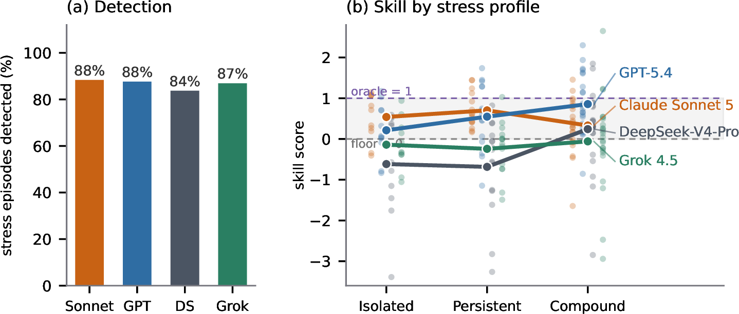
All four models see the hidden world about equally well (Table 3, Figure 4a). Each detects 84–88% of its stress episodes, with a mean lag of 0.32–0.42 weeks: when a factor enters a stress regime, its symptoms are typically named in the rationale within the same week. The two models that end up below the base-stock floor on cost have the shortest detection lags. Whatever separates these models on this task, it is not state estimation.
Skill scores, in contrast, diverge widely (Table 2, Figure 4b). Claude Sonnet 5 and GPT-5.4 recover 49% and 62% of the floor-to-oracle cost gap overall and beat the base-stock floor’s raw cost on 40 and 42 of 50 seeds. DeepSeek-V4-Pro and Grok 4.5 score \(-0.23\) and \(-0.13\), falling below the floor on 22 and 28 of their 49 scoreable seeds: on roughly half their tapes, a symptom-blind base-stock rule with the same action menu would have been cheaper than acting on their (largely correct) diagnoses. Along the stress axis the field splits three against one. GPT-5.4, DeepSeek-V4-Pro, and Grok 4.5 all post their best group on compound seeds (GPT-5.4 strongest at 0.86, with its weakest group isolated at mean 0.21, median 0.07), while Claude Sonnet 5 is the exception: strongest on persistent (0.70, no seed below the floor) and weakest on compound, where seven of its nine below-floor seeds sit. DeepSeek’s compound mean is pulled up by a single outlier tape; its group median is 0.32. Individual scores above 1 occur (33 of 196 scoreable runs) and are legitimate, since the oracle is Bayes-optimal in expectation but not per-tape. Even the best model leaves over a third of the gap to a policy computed from identical observations, so the benchmark is far from saturated.
The knowing-doing rate (Table 3) shows where correct diagnosis fails to prevent empty shelves. For every model the rate peaks on persistent seeds, at 0.34–0.43, versus 0.07–0.24 on isolated seeds: when a disruption lasts many weeks, a correctly diagnosed stress week still ends in stockout roughly four times in ten. Brief shocks are handled; sustained ones convert knowledge into cost. The rate is not a model ranking, however: read across models it runs opposite to skill, with the near-best model (Claude Sonnet 5) highest and the worst (Grok 4.5) lowest. The reason is that a stockout-based rate sees only one face of the gap. An agent can fail on a correct diagnosis by under-responding, stocking out despite naming the problem, or by over-responding, buying so much premium protection that stockouts are rare while the bill exceeds what the symptom-blind floor would have paid. The two models below the floor fit the second face: their diagnosed-week stockout rates are the lowest of the four while their total costs are the highest. We quantify the response taxonomy only for the two above-floor models (below); for the two below it, the mechanism rests on trace readings like Exhibit B in Appendix D, not on a measured cost decomposition. Two further qualifications keep the rate from reading as a week-level fault measure. A stockout in a given week can stem from an ordering decision made weeks earlier. And Table 4 shows a severity confound: stressed weeks the agent correctly diagnosed stock out more often than stressed weeks it missed, for every model, because weeks bad enough to be noticed are also bad enough to strain the shelf. The knowing-doing rate therefore says that correct diagnosis does not guarantee protection; it does not say that diagnosis causes stockouts, and we do not rank models on it.
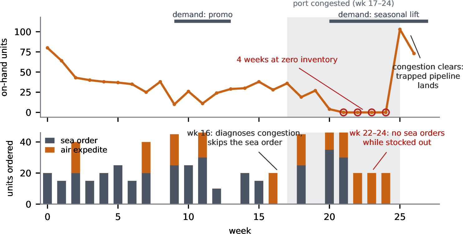
Reading the traces suggests the models fail in opposite directions; full excerpts are in Appendix 10. Claude Sonnet 5 on seed 1 (persistent; port congested weeks 17–24 while demand lifts) freezes: it diagnoses the congestion in week 16 and skips its sea order at once; the orders it does place are held up behind the blocked port, and through weeks 22–24, at zero inventory, it stops ordering by sea entirely (Figure 5 in the appendix plots the full episode). By week 22 it has held zero inventory for two weeks, yet writes “I already have a very large pipeline: 104 units in transit …ordering more now would only add to an already oversized pipeline …given berth_wait is still elevated (15 days)” and orders nothing, counting units trapped behind the congestion it itself diagnosed as usable cover. It ends with four consecutive zero-inventory weeks costing $660–$823 each, while the oracle keeps placing modest orders that arrive after the congestion clears. DeepSeek-V4-Pro on seed 25 (isolated; a two-week canal closure) flails: within two weeks of a correct diagnosis it locks freight rates for four weeks, air-expedites units, and stacks 80 units of orders against \(\sim\)20-per-week demand, on top of 117 already in transit. The closure ends in week 5; the fees and holding costs it bought persist, and the episode finishes at skill \(-1.45\); the costly response outlived the two-week shock it answered. Neither trace contains a detection error. The two directions generalize beyond these seeds. In every one of Claude Sonnet 5’s nine below-floor seeds, its spending on air expedite alone exceeds its entire excess over the floor, and about nine in ten of its air orders on those seeds coincide with a genuine disruption: it over-doses real problems rather than chasing noise. GPT-5.4 errs the other way, structurally under-using the mitigation levers: it never locks freight rates in 87% of the seeds containing a freight spike and never orders a batch inspection in 63% of the seeds with quality escapes, while naming those conditions in its rationales.
6 Discussion and Limitations↩︎
The results support one claim: on this task, frontier-model failures are concentrated in control, not state estimation, and the fair oracle makes that split measurable. A privileged oracle could not have licensed it, because any shortfall could be attributed to the information gap rather than to policy. The fairness itself carries one disclosed asymmetry. The oracle receives the identical observation stream and never the hidden state, but its filters use the true generative parameters (regime means, transition probabilities), while the LLM sees only a qualitative world description. Skill \(=1\) therefore means “Bayes-optimal given the true model”, a demanding but not information-free reference, and scores above 1 are possible and observed.
The belief metrics read stated beliefs, and stated belief is a lower bound. Detection is measured from the rationale the model writes, not from its internal state; a model may track a factor it never mentions. This biases detection down, which strengthens the seeing-vs-doing contrast, but the knowing-doing rate inherits the grader’s labels. A stratified manual read found the labels correct on the sampled metric-relevant weeks, and an independent second grader agrees with the production grader on the metric-relevant component (which named factors intersect true stress) at 89%; residual disagreement sits on calm-week over-labels, which cannot enter the knowing-doing rate by construction. Both audits sampled the original twenty-seed grading run; all later grading (the thirty expansion seeds and the additional models) used the identical configuration but was not freshly audited.
Two design choices qualify behavioral readings of the traces. Once a second supplier contract is signed, the world offers no way to end it (the lapse action affects only unsigned offers), so the weekly dual-sourcing fee is unavoidable from that point on, for every agent, and paying it is not by itself a decision error. And the two paid intelligence levers (audit and briefing) return near-deterministic ground truth by design, so what varies across models is how often they are consulted, not how well their output is read.
The cost-side numbers rest on single runs. Each model–seed cell is one run, and provider-side nondeterminism is unquantified. Group means pool 11–23 seeds, and the cross-model contrasts (a 0.85-point overall skill spread against detection rates within four points of one another) are far larger than plausible single-run noise, but per-seed values should be read as samples, not estimates. The oracle reference is a 20-replication mean with standard error 0.2–1.8% of the reference cost.
Finally, the benchmark covers one domain, one SKU, one prompt arm, and four models. The tapes are generated from published seeds rather than scraped, so they cannot occur in training data, but conclusions about why the gap concentrates on persistent stress await intervention: prompt arms that coach explicit belief maintenance, repeated runs per cell, a clairvoyant ceiling to bound the oracle’s optimality gap, and a broader model set.
Appendix↩︎
7 World and Cost Parameters↩︎
All values below are read directly from the environment source; they fully specify the weekly cost function and the six hidden factor processes of Section 3.
7.0.0.1 Costs.
Each week’s cost is the sum of the applicable components:
| Component | Charge | When |
|---|---|---|
| Sea shipping | $4.00 (Suez) / $6.00 (Cape) per unit \(\times\) freight mult. | at dispatch |
| Supplier price delta | qualified \(+\)$1.00, spot \(-\)$1.50, backup \(+\)$0.30 per unit | at dispatch |
| Holding | $1.00 per unit-week, on hand and in transit | weekly |
| Stockout | $20.00 per unit of unmet demand (lost sales) | weekly |
| Port demurrage | $2.00 per unit held at a blocked port | while blocked |
| Quality rework | $15.00 per defective unit landed | at arrival |
| Diversion surcharge | $2.00 per unit forced from Suez around the Cape | at diversion |
| Crisis back-order | $60.00 per unit a supplier shorts during a canal event | coupled |
| Air expedite | $15.00 per unit, at most 20 units/week | on use |
| Briefing / audit / inspection | $30 / $25 / $40 flat per call | on use |
| Dual-sourcing overhead | $4.00 per week while two or more contracts are live | weekly |
Orders are capped at 100 units per week. Sea lead times are 3 weeks via Suez and 4 via the Cape; air freight lands the following week. The implied newsvendor critical ratio is \(20/21 \approx 0.95\), which fixes the base-stock safety factor \(z \approx 1.67\) used by the floor policy.
7.0.0.2 Factor processes.
Each factor is an independent Markov chain stepped from the seed’s random stream before any action applies. Starred regimes are the stress regimes that define episodes in Section 4.
| Factor | Regimes | Key dynamics and observations |
|---|---|---|
| Demand | normal, promo spike\(^{*}\), seasonal lift\(^{*}\), structural decline\(^{*}\) | onsets 0.03/0.015/0.005 per week; promo lasts 4 weeks, seasonal persists 0.85 (cap 8), decline persists 0.97. Weekly means 20/26/30/14 units; observed point-of-sale and forecast carry Gaussian noise (sd 4 and 6). |
| Supplier | reliable, wobbling, degraded\(^{*}\), defunct\(^{*}\) | onset 0.10, wobbling\(\to\)degraded 0.45; degraded recovers within 4 weeks or dies (0.06). Scorecard band reads one severity level better than the truth; lead-time slip and fill fraction are noisy. |
| Freight | slack, normal, tightening, spike\(^{*}\) | tightening onset 0.06, tightening\(\to\)spike 0.18, spike persists 0.80 (cap 6). Rate multipliers 0.7/1.0/1.8/4.0; index and outlook noisy. |
| Port | clear, building, congested\(^{*}\), customs hold\(^{*}\) | building onset 0.06, building\(\to\)congested 0.30, congested persists 0.85 (cap 8); customs holds last about a week. Berth wait rises from \(\sim\)1 to \(\sim\)16 days; a blocked port delays every arrival one week. |
| Quality | in control, drifting, out of control\(^{*}\) | drift onset 0.04; the drift-to-failure hazard grows with age (\(0.05 + 0.04 \cdot \text{age}\)). Defect fractions 0.1%/2%/6%; observed only as a noisy accept/marginal/reject inspection band. |
| Canal | calm, watch, disruption\(^{*}\), recovery, false alarm | calm\(\to\)watch 0.08; watch resolves to a real closure (0.50) or a false alarm (0.20). Transit counts are exact but the first closure week and a false alarm emit the identical “crash” reading. A closed canal queues Suez ships, then diverts them (\(+\)3 weeks, Cape rate, surcharge). |
8 Reference Policy Details↩︎
8.0.0.1 Base-stock floor.
Order-up-to level \(S = \mu L + z\sigma\sqrt{L}\) with \(\mu = 20\), \(\sigma = 4\), \(L = 4\) (3-week Suez lead plus one review week), \(z = \Phi^{-1}(20/21) \approx 1.67\). Every week it orders \(\max(0, S - \text{inventory position})\), always via Suez from the same supplier, and never touches a lever or reads a symptom.
8.0.0.2 Oracle decision loop.
Each week the oracle (i) updates one exact forward Bayes filter per factor on the shared observation dictionary; (ii) samples \(\sim\)200 joint futures of all six factors from the filter posteriors, rolled forward to the episode’s final week with the true transition tables; (iii) scores a small candidate menu against every sampled future using a fast surrogate of the cost function, holding future weeks to a base-stock continuation; and (iv) executes the cheapest candidate through the world’s action methods, the same calls that back the LLM’s tools. The candidate menu contains order quantities {0, four weeks, six weeks of expected demand}, both routes, the contracted suppliers, and each mitigation lever gated on posterior risk (freight lock if \(\Pr(\text{tightening or spike}) > 0.3\); air expedite if port risk \(> 0.3\); inspection if quality risk \(> 0.5\) and a batch lands next week). The same sampled futures are reused across candidates (common random numbers). The oracle never buys briefings or audits; the LLM may. A seed’s reference value is the mean of 20 such runs; replications vary both the random stream and the per-decision trajectory budget (191–210 sampled futures, hence the \(\sim\)200).
9 Belief Grading Details↩︎
The grader (gpt-5-mini via OpenRouter, temperature 0, reasoning effort capped at low) receives only the week’s rationale text and the fixed six-name factor vocabulary, and returns strict JSON. Its instructions require a factor to be labeled only if the text claims it is a problem that week: ruled-out or benign mentions do not count, factual symptom reports do count, and precautions without a current problem do not count. Mean detection lag is computed over detected episodes only; naming a factor before its episode starts never counts as detection. The search then runs forward to the end of the trace, so a mention long after onset still counts, as a slow detection of that episode; in the measured runs mean lag is under half a week, so detections overwhelmingly land at or just after onset. In the knowing-doing rate, “stockout” means the week’s available stock (inventory plus arrivals) fell short of realized demand. Validation: on a stratified 30-row manual read, all 10 sampled hit-class labels were correct and 9 of 10 sampled misses were genuine (the tenth ambiguous, in the direction that understates detection); an independent second grader (Claude Haiku 4.5, same prompt, 100 sampled weeks) agreed 43% on exact label sets but 89% on the metric-relevant quantity, the intersection of labeled and truly stressed factors. Calm-week over-labels, where graders disagree most, are excluded from every reported metric by construction.
The grader’s full instructions are reproduced below; {rationale} is replaced by the week’s rationale text.
10 Seed Timelines and Trace Excerpts↩︎
The table below gives the ground-truth stress windows for the nine originally released seeds, obtained by replaying each tape with no actions (the tape is action-independent). Each entry reads factor: regime, weeks active; factors are the six of Section 3. Windows joined by “\(+\)” overlap in time — the defining feature of the persistent and compound groups. Timelines for the forty-one expansion seeds ship with the released tapes.
| Seed | Group | True stress windows (weeks active) |
|---|---|---|
| 157 | isolated | canal closed 12–13; quality out of control 23–24; freight spike 25–26 |
| 25 | isolated | canal closed 4–5; port customs holds 6–7, 12, 21, 26; supplier degraded wk 20 |
| 112 | isolated | demand shifts only: decline 13–14, seasonal lift 20–24 |
| 1 | persistent | port congested 17–24 \(+\) demand seasonal lift 20–26 \(+\) freight spike wk 19; demand promo 9–12 |
| 172 | persistent | port congested 5–11 \(+\) demand promo 9–12; demand seasonal lift 22–26 \(+\) supplier degraded 24–26 |
| 170 | persistent | freight spike 3–8 \(+\) port congested 5–12; demand promos 2–5, 15–18; freight spike 24–26 \(+\) supplier degraded wk 26 |
| 21 | compound | demand seasonal lift 10–17; port customs hold wk 11; then canal closed 21–26 \(+\) quality out of control 22–24 \(+\) supplier degraded wk 23 |
| 143 | compound | freight spike 5–10 running into port congestion 10–17; supplier degraded 2–5; port customs hold wk 1; canal closed wks 15, 25 |
| 99 | compound | the marathon tape: two port-congestion runs plus a customs hold, two canal closures, three demand-regime changes, supplier degraded 23–24 |
10.0.0.1 Exhibit A: freezing (Claude Sonnet 5, seed 1).
Week 16, on diagnosing the congestion: “Port congestion has spiked severely (berth_wait 10 days…) …I’ll skip placing a new sea order this week …and reassess next week once conditions hopefully ease.” Week 22, with zero on-hand inventory and a stockout in progress: “Despite the current 0 on-hand inventory, I already have a very large pipeline: 104 units in transit (arriving weeks 23–25) …roughly 4–5 weeks of cover …ordering more now would only add to an already oversized pipeline, incurring extra holding/in-transit costs and demurrage risk given berth_wait is still elevated (15 days).” Weeks 21–24 all close at zero inventory ($660–$823 per week).
10.0.0.2 Exhibit B: flailing (DeepSeek-V4-Pro, seed 25).
Week 4: “Week 4: Disruption confirmed — Suez counts crashed to 28/25 …Cape is now the only safe route. Locked freight at 1.02x for 4 weeks. Ordering 40 via Cape/spot …” Week 6, correctly closing the diagnosis: “Week 6: Suez reopening — counts back to 56/56 …” By then the freight lock, air expedite, and stacked orders are sunk; weekly costs run $610–$814 through week 8, and the episode ends at $7,950 total cost, skill \(-1.45\).
11 Agent Interface: Prompt and Observation Format↩︎
11.0.0.1 Weekly observation.
The observation dictionary below is serialized into the agent’s context each week, exactly as produced by the environment (a presentation-manifest key used only by the web frontend is omitted). This example is week 10 of seed 1 under the base-stock policy: the demand promo is active (point-of-sale 29 against a baseline of 20), the lane is calm, and the symptom-blind policy has just taken a small stockout.
11.0.0.2 System prompt (FAITHFUL arm).
The complete system prompt used for all 200 runs is reproduced verbatim below. It specifies mechanics, costs, tool semantics, and the latent structure of each factor, and contains no strategy advice; its inclusion substantiates the rules-only claim of Section 3.
References↩︎
An earlier circulated draft reported DeepSeek-V4-Pro on a twenty-seed subset: a fault in the belief-grading pipeline had silently read stale run files for the remaining seeds. All numbers here are from complete fifty-seed runs, regraded and rescored.↩︎