The SIGReg Objective as Variational Free Energy:
A Theoretical Active-Inference Account of JEPA World Models
July 15, 2026
Abstract
Joint-Embedding Predictive Architectures (JEPAs) are the dominant design for latent world models, yet they are usually justified by empirical performance rather than a normative principle. We show that the choice of anti-collapse regulariser determines whether a JEPA’s training objective, a prediction loss plus a weighted embedding regulariser, is a valid Active Inference (AIF) variational free energy. We organise four non-contrastive regularisers (VICReg, LogDet, PairDist, and SIGReg) into an entropy-estimator hierarchy indexed by a prior-miscalibration gap, and show that the gap’s sign, whether the estimator bounds the latent entropy from above or below, decides whether the AIF surprise bound survives: VICReg and LogDet are unsafe upper bounds, PairDist a safe lower bound, and SIGReg eliminates the gap. We then prove a correspondence theorem: under the standard constant-noise encoder model and successful SIGReg enforcement (isotropic-Gaussian embeddings), the gap vanishes, the objective becomes an exact information bottleneck, the surprise bound is preserved, and the latent goal cost becomes an exact proxy for AIF pragmatic value, whereas VICReg leaves an irreducible second-order anisotropy term. We extend the correspondence to multi-step expected free energy, ensemble epistemic value, and a learned-policy regime, and we identify the one AIF term no current JEPA world model computes: the state-epistemic value, a future-state coverage signal. The predictions differ in kind, not degree, and are stated here as theoretical consequences left for empirical test in separate work; full proofs are in Appendix sec:sec:app:proofs?, and the algebraic core of every result is machine-verified in Lean 4 (Appendix sec:sec:app:lean?).
1 Introduction↩︎
Active Inference (AIF) and Joint-Embedding Predictive Architectures (JEPA) are two independently developed accounts of how an agent can learn and act from high-dimensional observations. AIF, rooted in the Free Energy Principle [1], is normative: the agent maintains a generative model and acts to minimise variational free energy, an upper bound on sensory surprise. JEPA, developed within the self-supervised learning (SSL) tradition [2], is architectural: a deterministic encoder maps observations to latent embeddings and a predictor models the dynamics in that latent space, avoiding pixel-level reconstruction.
Despite their separate origins, both frameworks factor the learning objective into the same two competing terms: a complexity term that penalises departures from the dynamics model and an informativeness term that rewards capturing useful structure in observations. The Information Bottleneck (IB) principle [3] formalises this trade-off as a Lagrangian \(\mathcal{L}_{\mathrm{IB}} = \mathcal{D}[\text{encoder}\,\|\, \text{prior}] - \hat{I}(Z;X)\), where the divergence \(\mathcal{D}\) and the information estimator \(\hat{I}\) vary across implementations. In AIF the informativeness term is a likelihood or a mutual-information bound [4], [5]. In JEPA world models it is maintained implicitly by an anti-collapse regulariser such as VICReg [6]. The shared structure invites a precise question: how exactly do the terms of a JEPA world model’s training loss correspond to the terms of the AIF variational free energy?
1.0.0.1 The problem: non-contrastive informativeness is approximate.
The answer hinges on how the informativeness term is maintained. The contrastive route [4] estimates mutual information with an InfoNCE lower bound [7], so the agent never overstates its own informativeness and the free-energy bound is preserved by construction, at the cost of stochastic encoders and a learned critic. Every deployed JEPA world model [8]–[11] instead uses a deterministic encoder with a non-contrastive regulariser. Under the standard constant-noise model [12], maximising informativeness then reduces to maximising the marginal differential entropy \(h(Z)\), which is intractable in high dimension. VICReg approximates it through the first two moments [13], introducing a gap between the true entropy and its proxy. Crucially, this gap is not merely a matter of degree: VICReg’s proxy is an upper bound on the Gaussian reference entropy (via Hadamard’s inequality), which is itself an upper bound on \(h(Z)\) (via the maximum-entropy theorem). Maximising an upper bound provides no guarantee that the true entropy increases, since the optimiser can inflate the proxy without increasing \(h(Z)\), whereas increasing a lower bound is safe. This bound-type asymmetry is the theoretical motivation for seeking tighter estimators.
1.0.0.2 Contributions.
We make two linked contributions. (1) An entropy-estimator hierarchy (Section 4.1). We cast four non-contrastive regularisers (VICReg [6], LogDet [13], PairDist [14], and SIGReg [15]) as a monotone elimination of prior-miscalibration sources. The organising result is a three-source gap decomposition (Proposition 1): every
covariance-based entropy proxy is loose through a non-Gaussianity gap, an off-diagonal-covariance gap, and an estimation error, each with an explicit zero condition and the first two with a definite sign. The hierarchy also separates two axes, bound
type (upper/unsafe vs.lower/safe) and distributional enforcement, and shows SIGReg is the first estimator that is simultaneously safe and exact. (2) The SIGReg–AIF correspondence (Section 4). We
prove that replacing VICReg with SIGReg upgrades the AIF correspondence from approximate to exact (Theorem 1): under the constant-noise model and successful
SIGReg enforcement, the gap vanishes (\(\Delta_{\mathrm{SIG}}=0\)), the loss admits an exact IB decomposition, and the AIF bound \(F\ge-\ln p(x)\) is preserved (the first non-contrastive
regulariser to achieve this). A dual-tightening corollary (Corollary 1) shows isotropy simultaneously closes the entropy gap and the KL–MSE approximation error, making the latent
goal cost an exact AIF pragmatic-value proxy (Proposition 5). We then extend the correspondence from the single-step free energy \(F\)
to the multi-step expected free energy \(G\), to ensemble-based epistemic value, and to a learned-policy regime, and we isolate the one AIF term no current JEPA world model computes: the state-epistemic value, a
future-state coverage signal (Proposition 6). Following [16], the
algebraic core of both contributions is machine-verified in the Lean 4 theorem prover, compiling with zero sorry obligations (Appendix 9).
1.0.0.3 What the correspondence buys.
The equivalence is not a relabelling, because it delivers what the two adjacent results (that JEPAs already learn approximately isotropic-Gaussian embeddings [17] and that this makes their latents identifiable and plannable [16]) do not. First, it gives a validity criterion for the objective: whether the surprise bound \(F\ge-\ln p(x)\) survives is a property of the estimator’s bound direction (Proposition 2), separate from how Gaussian or identifiable the embeddings are. Second, it equips JEPA world-model planning with a principled epistemic-value term, the information gain that deployed planners currently approximate only heuristically through ensemble disagreement [8]. Third, it turns the heuristic “add an exploration bonus” into a specific, signed prescription, the state-epistemic coverage term isolated above. Fourth, it unifies the deployed non-contrastive JEPA world-model ecosystem with deep active inference, so each can import the other’s tools. The bare correspondence is the mechanism and these consequences are the contribution.
1.0.0.4 The falsifiable hook, and a caveat.
The distinction is sharp because it is qualitative: under SIGReg the prior-miscalibration gap is exactly zero and the goal metric is exactly isotropic, while under VICReg both carry an irreducible \(\mathcal{O}(\delta^2)\) anisotropy term. This produces predictions that differ by kind, not degree (e.g.,the embedding condition number \(\kappa\!\approx\!1\) vs.\(\kappa\!\gg\!1\)). The Gaussianity result noted above, that any successfully trained JEPA already learns approximately Gaussian embeddings [17], does not blunt this distinction, for three reasons the theory makes precise: “approximately Gaussian” is not sufficient for the AIF bound, which is binary in the estimator’s type (Proposition 2), so VICReg may fail to preserve it even when the residual is small; the theory governs the training path, not only the optimum; and the bridge is independently valuable (Section 5 expands all three). A second concurrent result [16] supplies the precondition under which latent distances are physically meaningful (Section 4.6) and triangulates the isotropic-Gaussian target from a third, independent direction.
1.0.0.5 Organisation.
Section 2 surveys related work; Section 3 fixes notation and three published facts; Section 4 develops the hierarchy, the correspondence theorem, the multi-step/EFE and learned-policy extensions, and the testable predictions the theory entails. Empirical validation of these predictions is left to separate work; the present paper is confined to the theoretical development. Section 5 concludes.
2 Related Work↩︎
2.0.0.1 JEPAs and latent world models.
Joint-embedding prediction has become the dominant SSL design for control-capable world models [2]. Image and video variants such as I-JEPA and V-JEPA, and the action-conditioned V-JEPA 2 [10], learn predictors in a frozen or slowly-updated latent space; DINO-WM [9] plans zero-shot on frozen DINOv2 features; PLDM [8] trains an end-to-end latent dynamics model with a VICReg-style anti-collapse term and an ensemble disagreement cost; and TD-JEPA [18] extends latent prediction to zero-shot reinforcement learning. [19] ablate the design space and report that cross-entropy-method planning with an L2 terminal cost is the strongest planner and that a short two-step training rollout is best. Most relevant here, LeWorldModel [11] is the first JEPA world model to train stably end-to-end from raw pixels using SIGReg as the sole anti-collapse regulariser, with a two-term objective, no exponential-moving-average teacher, and CEM-based model-predictive control, precisely the system our theory formalises. Complementing these architectures, [16] ask when a JEPA trained this way earns the name “world model” at all, and prove that alignment plus Gaussian regularisation recovers the world’s latent degrees of freedom up to a linear map. Their identifiability result is the precondition under which latent distances become physically meaningful, and we return to it in Section 4.6.
2.0.0.2 Non-contrastive SSL regularisation.
A family of regularisers prevents representational collapse without negative pairs by shaping the embedding covariance: VICReg’s variance/covariance terms [6], Barlow Twins’ redundancy reduction [20], and Whitening [21]. [13] recast VICReg’s variance/covariance terms as a Gaussian entropy estimator and place it alongside a tighter log-determinant (LogDet) estimator. [14] provide a non-parametric pairwise-distance entropy bound (PairDist). SIGReg [15] departs from moment matching entirely, enforcing an isotropic-Gaussian distribution by random-projection Gaussianity testing and recovering VICReg as a degenerate moment-matching special case. We unify these under a single axis: the quality of the implicit AIF prior, i.e.the direction and tightness of the entropy bound and hence whether the AIF surprise bound survives, and supply the information-theoretic reason to prefer SIGReg. This bound-safety ordering is distinct from the Gaussianity-strength hierarchy of [16], which ranks the same regularisers (implicit, second-moment, full) by how strongly they drive the embeddings toward Gaussian. Instead, ours orders by whether the variational bound is preserved, not by how tight the distributional constraint is. Beyond self-supervised pretraining, the same isotropic-Gaussian regularisation has independently been used to stabilise deep reinforcement learning under non-stationarity, mitigating representation collapse and plasticity loss [22]. This is external evidence, in a control setting, that the isotropic-Gaussian structure our correspondence relies on carries concrete downstream benefits.
2.0.0.3 Active inference and deep generative agents.
AIF [1], [23] casts perception and action as free energy minimisation. Deep instantiations scale it with amortised inference and learned dynamics: Monte-Carlo deep active inference [24], the deep-learning treatment of [5], and Contrastive Active Inference [4], which replaces the intractable decoder with an InfoNCE critic and is, to our knowledge, the only prior route that achieves an exact AIF correspondence in a latent model. Latent-imagination control such as Dreamer [25] shares the rollout-and-score structure but is not framed as free-energy minimisation. Two concurrent variational JEPAs recover an AIF reading by building probabilistic structure into the architecture: Var-JEPA [26] reformulates JEPA as a coupled variational autoencoder and derives an information-bottleneck decomposition by ELBO surgery, while the separately-authored VJEPA of [27] (distinct from Meta’s V-JEPA) equips the predictor with a learned covariance and a KL-to-prior term and proves an objective-side collapse-avoidance result. Both are, in our terms, the easy case, i.e., they build in the very stochasticity active inference presupposes, and, as [27] makes explicit, model belief dynamics only, omitting the sensory likelihoods, preferences, and policy evaluation that a full active-inference agent requires. The contribution of this paper is the hard case: the deterministic, non-contrastive architecture that every deployed JEPA actually instantiates, in which the probabilistic structure must be recovered rather than assumed. It further supplies the expected-free-energy layer that these belief-only formulations leave out, namely pragmatic value, epistemic value, and policy-as-inference. Where [4] establish one route to exact latent AIF, the contrastive one built around an InfoNCE critic, our result covers the route the deployed JEPA world-model ecosystem already instantiates (V-JEPA 2, DINO-WM, PLDM, LeWorldModel) and states the condition under which that objective is a valid free energy. Two results from model-based control bear on our learned-policy regime (Section 4.5). [28] show that a well-regularised world model induces a smoother optimisation landscape than the true dynamics, making first-order policy extraction effective where gradient-free planners (CEM, MPPI) are the default; our correspondence supplies the regulariser-side condition they leave open, since the embedding condition number \(\kappa\) measures that conditioning and only isotropy drives it to one. [29] show that the optimal goal-reaching cost-to-go is a quasimetric, asymmetric because reachability is irreversible. This does not contradict Proposition 5, since pragmatic value is a log goal prior and preferences over states are symmetric by construction, but it does bound the regime in which the goal cost may be read as a value estimate (Section 5.1).
2.0.0.4 Information bottleneck and mutual-information estimation.
The IB principle [3] underlies both deep variational IB [30] and multi-view IB [31]. [32] survey variational MI bounds, and [12] expose the degeneracy of MI for deterministic encoders, the issue that the constant-noise model resolves and that motivates the entropy-maximisation view we adopt. The same work documents two further IB pathologies: the failure to recover the IB curve under deterministic targets and the degenerate landscape of the IB Lagrangian. Neither bears on the present construction, because our informativeness term is a single entropy quantity \(h(Z)\) rather than a \(\beta\)-weighted IB trade-off whose curve must be recovered; we maximise one entropy under a distributional constraint, not a two-term information trade-off. Relative to all of the above, our contribution is to make the JEPA/AIF correspondence exact for a non-contrastive, deterministic encoder by controlling the prior-miscalibration gap, and to trace the consequences through multi-step planning. Because the JEPA line of work shares authorship, Appendix 8 states precisely how this paper differs from each prior result and discusses the relevance of the active-inference perspective it introduces.
3 Background↩︎
3.0.0.1 Notation.
All logarithms are natural. The latent space is \(\mathcal{Z}=\mathbb{R}^d\) and the observation space is \(\mathcal{X}\). An encoder \(f_\phi:\mathcal{X}\to\mathcal{Z}\) maps an observation \(x_t\) to an embedding \(z_t=f_\phi(x_t)\), and a predictor \(P_\xi:\mathcal{Z}\times\mathcal{A}\to \mathcal{Z}\) produces \(\hat{z}_t=P_\xi(z_{t-1},a_{t-1})\). We write \(q_\phi(s_t\mid x_t)\) for the encoder/posterior, \(p_\xi(s_t\mid s_{t-1},a_{t-1})\) for the transition prior, \(h(\cdot)\) for differential entropy, \(I(\cdot;\cdot)\) for mutual information, and \(D_{\mathrm{KL}}\!\left[\cdot\,\middle\|\,\cdot\right]\) for the Kullback–Leibler divergence. Throughout, \(\mathcal{O}(\cdot)\) denotes the Landau (big-\(O\)) order symbol.
3.0.0.2 Fact 1 (AIF free energy).
An AIF agent minimises the variational free energy, which decomposes as [5], [23] \[F \;=\; \underbrace{D_{\mathrm{KL}}\!\left[q_\phi(s_t\mid x_t)\,\middle\|\,p_\xi(s_t\mid s_{t-1},a_{t-1})\right]} _{\text{complexity}} \;-\; \underbrace{\mathbb{E}_{q_\phi}\!\left[\log p(x_t\mid s_t)\right]}_{\text{accuracy}}. \label{eq:vfe}\tag{1}\] Replacing the intractable decoder by a mutual-information term and adding \(\log p(x_t)\) yields the equivalent MI-form \(F^{+}=D_{\mathrm{KL}}\!\left[q_\phi(s_t\mid x_t)\,\middle\|\,p(s_t)\right]-I(S_t;X_t)\), an instance of the IB Lagrangian [3], [4]. The informativeness term \(I(S_t;X_t)\) is generally intractable; how it is estimated determines the agent’s prior calibration.
3.0.0.3 Fact 2 (constant-noise encoders).
A strictly deterministic encoder gives a degenerate \(I(Z;X)=+\infty\). The standard remedy [12] adds fixed, small, isotropic observation noise, \(Z=f_\phi(X)+\epsilon\) with \(\epsilon\sim\mathcal{N}\!\left(0,\sigma^2_{\mathrm{noise}}I_d\right)\), so that the conditional entropy is a constant \(C_{\epsilon}=\tfrac{d}{2}\ln(2\pi e\,\sigma^2_{\mathrm{noise}})\) independent of \(\phi\). Then \(I(Z;X)=h(Z)-C_{\epsilon}\), and \[\arg\max_\phi I(Z;X) \;=\; \arg\max_\phi h(Z). \label{eq:io-entropy}\tag{2}\] Maximising AIF informativeness is therefore equivalent to maximising the marginal differential entropy of the embeddings; any regulariser that maintains \(h(Z)\) serves as the informativeness proxy. The status of \(\sigma_{\mathrm{noise}}\) as an interpretive device rather than a property of deployed JEPAs is discussed in §5.1.
3.0.0.4 Fact 3 (VICReg as an upper-bound entropy proxy).
[13] show that VICReg’s variance/covariance terms constitute the Gaussian entropy estimator \(\hat{H}_{\mathrm{VR}}(Z)\approx\tfrac{1}{2}\sum_k\ln \hat{\sigma}^2_k\) (plus a constant). Combining Hadamard’s inequality [33] with the maximum-entropy theorem [34] gives the sandwich \[\underbrace{\hat{H}_{\mathrm{PD}}(Z)}_{\text{lower bound}} \;\le\; h(Z) \;\le\; \underbrace{\tfrac{1}{2}\ln|\Sigma|+C}_{=\,h_{\mathcal{N}}(Z)\;\text{(LogDet, tight UB)}} \;\le\; \underbrace{\tfrac{1}{2}\textstyle\sum_k\ln\sigma^2_k+C}_{\text{VICReg (loose UB)}}, \label{eq:bound-chain}\tag{3}\] where \(h_{\mathcal{N}}(Z)=\tfrac{1}{2}\ln|2\pi e\,\Sigma|\) is the Gaussian reference entropy and \(\Sigma=\operatorname{Cov}(Z)\). VICReg and LogDet bound \(h(Z)\) from above; PairDist bounds it from below. Maximising an upper bound is unsafe in the sense of Section 1.
3.0.0.5 The Gaussian bridge.
The complexity term connects to the prediction MSE used in practice through a standard Gaussian identity. For \(q_\varepsilon=\mathcal{N}\!\left(\mu_q,\varepsilon I_d\right)\) and \(p=\mathcal{N}\!\left(\mu_p,\sigma^2 I_d\right)\), \[D_{\mathrm{KL}}\!\left[q_\varepsilon\,\middle\|\,p\right] = \frac{1}{2\sigma^2}\|\mu_q-\mu_p\|_2^2 + \frac{d}{2}\!\left(\frac{\varepsilon}{\sigma^2}-1-\ln\frac{\varepsilon}{\sigma^2}\right), \label{eq:bridge}\tag{4}\] and since the second term is independent of \(\mu_p\), the optimiser sets coincide: \(\arg\min_\xi D_{\mathrm{KL}}\!\left[q_\varepsilon\,\middle\|\,p_\xi\right]=\arg\min_\xi\|\mu_q-\mu_{p_\xi}\|_2^2\) [35]. With \(\mu_q=z_t\) and \(\mu_{p_\xi}=\hat{z}_t\), the JEPA prediction loss \(\|\hat{z}_t-z_t\|^2\) is optimisation-equivalent to the AIF complexity term. When variances depart from isotropy by ratios \(1+\delta_k\), the residual is \(\mathcal{O}(\delta^2)\); this residual will be eliminated exactly under isotropy (Corollary 1).
4 Method: The SIGReg–AIF Correspondence↩︎
We first define the prior-miscalibration gap and decompose it (§4.1); we then state the single-step correspondence theorem (§4.2), extend it to multi-step planning and the expected free energy (§§4.3–4.4) and to a learned policy (§4.5), and finally derive the testable predictions (§4.7). The full proof development for the multi-step and expected-free-energy results is given in Appendix 6.
Table 1 fixes the correspondence at the level of objects: each Active Inference quantity, its JEPA world-model counterpart, and the equation in this paper where the identification is made. The table is the reading key for the rest of the section; the single row with no JEPA counterpart, the state epistemic value, is the paper’s central structural finding (Proposition 6).
| AIF object / role | JEPA counterpart | Defining relation |
|---|---|---|
| Hidden state \(s_t\) | Embedding \(\z_t=f_\phi(x_t)\) | encoder; Fact 1 |
| Observation \(x_t\) | Input observation | Raw sensory data \(x_t \in \mathcal{X}\) |
| Action \(a_t\) | Predictor action arg. (\(P_\xi:\Z\times\mathcal{A}\!\to\!\Z\)) | Control command \(a_t\in\mathcal{A}\) |
| Policy \(\pi\) | Action sequence / learned policy | §[sec:sec:method-policy] |
| Transition prior \(p(\z_\tau\mid \z_{\tau-1},a_{\tau-1})\) | Gaussian dynamics about \(P_\xi\) | Eq. [eq:genmodel] |
| Posterior \(q_\phi(\z_t\mid x_t)\) | Encoder \(+\) constant noise | Fact 2 |
| Complexity \(\KL{q_\phi}{p_\xi}\) | Prediction MSE (Gaussian bridge) | Eq. [eq:bridge] |
| Informativeness \(I(Z;X)\) | SIGReg-enforced \(\Istar\) | Def. [def:sigreg], Prop. [prop:sigzero] |
| Pragmatic value | Latent goal cost \(\|\z_\tau-\z_g\|^2\) | Prop. [prop:pragmatic] |
| Param.info gain | Ensemble predictive variance | §[sec:sec:method-efe-decomp] |
| State epistemic value \(h(Z_\tau\mid\pi)-\Ce\) | absent in JEPA | Prop. [prop:o2] |
5pt
4.1 The prior-miscalibration gap and the entropy-estimator hierarchy↩︎
Definition 1 (Prior-miscalibration gap). For an entropy proxy \(\hat{H}(Z)\) used in place of \(h(Z)\) in the AIF informativeness term, the prior-miscalibration gap is \(\Delta_{\hat{H}}(Z)\mathrel{\vcenter{:}}= h(Z)-\hat{H}(Z)\). A lower-bound proxy has \(\Delta\ge0\) (it underestimates achievable informativeness); an upper-bound proxy has \(\Delta\le0\) (it overpromises, and maximising it need not increase \(h(Z)\)).
Proposition 1 (Three-source gap decomposition). For any embedding distribution \(p_Z\) with finite covariance \(\Sigma\succ0\) and Gaussian reference entropy \(h_{\mathcal{N}}(Z)=\tfrac12\ln|2\pi e\,\Sigma|\), \[\Delta_{\hat{H}}(Z) = \underbrace{\bigl[h(Z)-h_{\mathcal{N}}(Z)\bigr]}_{\text{(I) non-Gaussianity}\;\le\,0} + \underbrace{\bigl[h_{\mathcal{N}}(Z)-\hat{H}(Z)\bigr]}_{\text{(II)+(III) estimation}} . \label{eq:gap-decomp}\qquad{(1)}\] Gap I is \(\le 0\) with equality iff \(p_Z\) is Gaussian (maximum-entropy theorem, [34] Thm. 8.6.5). For a variance-based proxy \(\hat{H}(Z)=\tfrac12\sum_k\ln\sigma^2_k+\tfrac d2\ln2\pi e\), the estimation gap contains an off-diagonal term \(\tfrac12\ln|\Sigma|-\tfrac12\sum_k\ln\sigma^2_k \le 0\) (Gap II), which is \(0\) iff \(\Sigma\) is diagonal (Hadamard’s inequality, [33] Thm. 7.8.1); the remaining term (Gap III) is the estimator’s own error and is \(0\) iff \(\hat{H}=h_{\mathcal{N}}\) exactly.
4.1.0.1 Scope of the decomposition, and two ways a gap can be absent.
The decomposition routes the total gap through the Gaussian reference \(h_{\mathcal{N}}\) and so characterises Gaussian-reference (covariance-based) proxies, namely VICReg and LogDet. An estimator that invokes no Gaussian reference does not incur Gaps I–II at all: PairDist [14] bounds the mixture entropy directly from pairwise distances between components, without moment-matching \(p_Z\) to a single Gaussian and without diagonalising \(\Sigma\), so its entire slack is Gap III. This is distinct from the gap’s zero condition holding. Gaps I and II vanish iff \(p_Z\) is Gaussian and \(\Sigma\) is diagonal respectively, which are properties of the distribution, not of the estimator; no estimator makes them true merely by declining to use them. Only SIGReg drives \(p_Z\) to satisfy them. Accordingly, Table 2 marks a gap not incurred when the estimator never invokes that source, and enforced when the estimator makes the zero condition hold. The hierarchy is monotone in the first sense (two sources incurred, then one, then none) and SIGReg alone supplies the second.
Insert \(\pm h_{\mathcal{N}}(Z)\) for ?? . Gap I follows from the maximum-entropy theorem; among distributions with covariance \(\Sigma\) the Gaussian uniquely maximises differential entropy. Gap II follows from Hadamard’s inequality \(|\Sigma|\le\prod_k\sigma^2_k\) with equality iff \(\Sigma\) is diagonal. Gap III is the residual by construction.
Proposition 2 (Bound type and AIF-bound preservation). Let \(\hat{F}^{+}\) be the proxy free energy obtained by substituting \(\hat{H}(Z)\) for \(h(Z)\). Then \(\hat{F}^{+}-F^{+}=\Delta_{\hat{H}}(Z)\), so: (i)* a lower-bound proxy (\(\hat{H}\le h\), e.g.PairDist) gives \(\hat{F}^{+}\ge F^{+}\ge-\ln p(x)\), so the AIF bound is preserved by construction; (ii) an upper-bound proxy (\(\hat{H}\ge h\), e.g.VICReg or LogDet) gives \(\hat{F}^{+}\le F^{+}\), which no longer certifies \(\hat{F}^{+}\ge-\ln p(x)\): the AIF bound is not guaranteed to be preserved. The inequality may still hold for a particular \(p_Z\); what is lost is the guarantee, and with it the licence to minimise \(\hat{F}^{+}\) as a surrogate for surprise. Maximising an upper bound is therefore unsafe rather than necessarily wrong: the slack \(\hat{H}-h\ge0\) can grow under optimisation (Remark 1).*
Remark 1 (Why an upper bound is unsafe: a worked case). The failure in Proposition 2(ii) is possible, not inevitable, and that possibility is precisely what makes an upper bound unsafe to maximise. Because \(\hat{H}-h\ge0\), an optimiser can raise \(\hat{H}\) by inflating the slack instead of the entropy. Let \(p_Z\) be uniform on an axis-aligned hypercube with per-coordinate variance \(\sigma^2\). Its off-diagonal covariances vanish and its marginal variances are \(\sigma^2\), so the VICReg proxy \(\hat{H}_{\mathrm{VR}}(Z)=\tfrac12\sum_k\ln\sigma^2_k+C\) assigns it exactly the value it assigns an isotropic Gaussian of the same variance. The true entropies differ, however: \(h(Z)=d\ln(\sqrt{12}\,\sigma)\) for the hypercube against \(h_{\mathcal{N}}(Z)=\tfrac d2\ln(2\pi e\sigma^2)\) for the Gaussian, and \(2\pi e>12\), so the hypercube is strictly sub-maximal by the full non-Gaussianity gap [15]. Maximising \(\hat{H}_{\mathrm{VR}}\) therefore exerts no pressure toward the entropy maximiser: the proxy can sit at its maximum while \(h(Z)\) does not. Nothing here forces \(\hat{F}^{+}<-\ln p(x)\) for any given input; what is lost is the certificate. A lower bound admits no such manoeuvre, since raising \(\hat{H}\le h\) can only raise \(h\).
4.1.0.2 The hierarchy.
Proposition 1 indexes four regularisers by which gap sources they incur, and Proposition 2 adds the orthogonal bound-type axis. Table 2 summarises the resulting hierarchy (Figures 2 and 4 render the bound-type sandwich and the two-dimensional design space). VICReg (diagonal Gaussian proxy) incurs Gaps I and II and is an unsafe upper bound; LogDet (full-covariance proxy) does not incur Gap II, but still incurs Gap I and remains an unsafe upper bound; PairDist (non-parametric) incurs neither, and is a safe lower bound, but it enforces no distributional shape; and SIGReg enforces the isotropic Gaussian directly, making all three zero conditions hold. Safety and enforcement are therefore independent properties, and only SIGReg has both.
| Level | Proxy | Bound type | Gap I | Gap II | Gap III |
| (non-Gauss.) | (off-diag.) | (estim.) | |||
| 0 | VICReg [6] | UB (loose) | incurred | incurred | — |
| 1 | LogDet [13] | UB (tight) | incurred | not incurred | small |
| 2 | PairDist [14] | LB | not incurred | not incurred | finite-\(N\) |
| 3 | SIGReg [15] | enforce. | enforced | enforced | enforced |
4pt
Definition 2 (SIGReg; [15]). Sketched Isotropic Gaussian Regularisation enforces \(p_Z\approx\mathcal{N}\!\left(0,I_d\right)\) by random-projection Gaussianity testing: for unit directions \(\mathbb{A}\subset\mathcal{S}^{d-1}\) and a univariate normality statistic \(T\) (the Epps–Pulley test, [36]), \(\mathrm{SIGReg}_T(\mathbb{A},\{z_n\})=\tfrac{1}{|\mathbb{A}|}\sum_{a\in\mathbb{A}} T(\{a^\top z_n\})\). The hyperspherical Cramér–Wold theorem [37] guarantees that matching all one-dimensional projections to a Gaussian is sufficient for a full distributional match.
Proposition 3 (SIGReg eliminates the gap). Under Fact 2, if SIGReg enforces \(p_Z=\mathcal{N}\!\left(0,\tfrac{c}{d}I_d\right)\), where \(c\mathrel{\vcenter{:}}=\operatorname{tr}(\Sigma_Z)\) is the target total variance, so the per-coordinate variance is \(c/d\), then \(h(Z)=h^{\star}(c,d)\mathrel{\vcenter{:}}=\tfrac d2\ln(2\pi e\,c/d)\), the gap is exactly zero (\(\Delta=0\) with Gaps I, II, III all zero), and the informativeness term attains its constrained maximum \(I(Z;X)=h^{\star}(c,d)-C_{\epsilon}\eqqcolon I^{\star}\). Gaussianity alone closes the gap (\(\Delta=0\)); isotropy additionally maximises the value of the closed bound.
4.2 The single-step correspondence theorem↩︎
Definition 3 (SIGReg-modular free energy). Under the constant-noise model with deterministic \(z_t,\hat{z}_t\), the SIGReg-modular free energy is \(F_{\mathrm{SIG}\text{-}\mathrm{mod}}=\tfrac{1}{2\sigma^2}\|\hat{z}_t-z_t\|_2^2+C_{\mathrm{KL}} -\lambda\,I^{\star}\,[1-\mathrm{SIGReg}_T(\mathbb{A},\{z_n\})]\), where \(C_{\mathrm{KL}}\) is the \(\mu_p\)-independent second term of the Gaussian bridge 4 and \(I^{\star}=h^{\star}(c,d)-C_{\epsilon}\) (Proposition 3); both are constants in \((\phi,\xi)\). This is the AIF reading of the LeJEPA objective \(\mathcal{L}_{\mathrm{LeJEPA}}= \|\hat{z}_t-z_t\|^2+\lambda_{\mathrm{SIG}}\,\mathrm{SIGReg}_T(\mathbb{A},\{z_n\})\) [15], up to \((\phi,\xi)\)-independent additive constants and the rescaling \(\lambda_{\mathrm{SIG}}=2\sigma^2\lambda\,I^{\star}\) (with \(I^{\star}>0\), i.e.\(c/d>\sigma^2_{\mathrm{noise}}\), which holds for the small fixed noise of Fact 2): once enforcement succeeds, the informativeness is not estimated but guaranteed* to equal the constant \(I^{\star}\) (Figure 1 renders this reading of the objective).*
Theorem 1 (SIGReg–AIF correspondence). Under the constant-noise model (Fact 2), the Gaussian encoder family, and successful SIGReg enforcement (\(p_Z=\mathcal{N}\!\left(0,\tfrac cd I_d\right)\) in the population limit \(M,N\to\infty\)), taking \(\lambda=1\) in Definition 3:
Zero gap. \(\Delta_{\mathrm{SIG}}\mathrel{\vcenter{:}}= h(Z)-h^{\star}(c,d)=0\); Gaps I, II, III all vanish.
Exact IB form (within the constant-noise model). \(F_{\mathrm{SIG}\text{-}\mathrm{mod}}\big|_{\mathrm{SIGReg}=0}=\tfrac{1}{2\sigma^2}\|\hat{z}_t-z_t\|^2+C_{\mathrm{KL}} -I^{\star}=F^{+}\), where the complexity term \(\tfrac{1}{2\sigma^2}\|\hat{z}_t-z_t\|^2+C_{\mathrm{KL}}\) equals \(D_{\mathrm{KL}}\!\left[q_\phi\,\middle\|\,p_\xi\right]\) exactly (not merely in gradient) because the Gaussian bridge 4 has zero anisotropy error under isotropy (Corollary 1), and the informativeness term equals \(I(Z;X)=I^{\star}\) exactly because SIGReg enforces the maximum-entropy distribution.
AIF bound preserved. \(F_{\mathrm{SIG}\text{-}\mathrm{mod}}=F^{+}\ge-\ln p(x)\). By contrast \(F_{\mathrm{VR}\text{-}\mathrm{mod}}\le F^{+}\) (Proposition 2(ii)), so under VICReg the bound is no longer guaranteed.
Contrastive equivalence. \(F_{\mathrm{SIG}\text{-}\mathrm{mod}}\) attains the same guarantees as the contrastive free energy \(F_{\mathrm{NCE}}\) [4] through the non-contrastive pathway.
From the MI-form \(F^{+}=D_{\mathrm{KL}}\!\left[q_\phi\,\middle\|\,p_\xi\right]-h(Z)+C_{\epsilon}\), enforcement gives \(h(Z)=h^{\star}(c,d)\) (Proposition 3), hence (i); isotropy makes the Gaussian-bridge 4 exact, and substituting it together with \(I(Z;X)=I^{\star}\) into the MI-form gives (ii) with all additive constants carried explicitly; (iii) follows from Proposition 2 at \(\Delta=0\); (iv) by comparison with the InfoNCE optimum. The multi-step extension and full derivations are in Appendix 6; Table 4 (§5.1) records which parts of this and the other main results are exact under the main-text assumptions and which are bounded or deferred.
Remark 2 (Which assumptions do the work). Theorem 1 is exact within its hypotheses, and it is worth naming what each one does. The constant-noise model (Fact 2) is what makes \(I(Z;X)\) well defined at all for a deterministic encoder, so it is presupposed by every information-theoretic statement here; it is assumed identically for VICReg and for SIGReg, and therefore does no work in the comparison between them. Successful SIGReg enforcement does the real work: it supplies \(p_Z=\mathcal{N}\!\left(0,\tfrac cd I_d\right)\) and with it, simultaneously, the zero entropy gap (i), the exactness of the Gaussian bridge (ii) via Corollary 1, and the bound preservation (iii). The population limit \(M,N\to\infty\) is what makes enforcement exact rather than approximate; at finite \((M,N)\) the guarantee degrades gracefully and linearly in the enforcement residual (Corollary 2), at the rate of Proposition 4, rather than failing discontinuously. Away from these conditions the correspondence is approximate, not void: Table 4 records the status result by result.
Corollary 1 (Dual tightening). Isotropy (\(\Sigma=\tfrac cd I_d\)) closes the entropy gap (Gap II) and the Gaussian-bridge approximation error simultaneously, because both are governed by the same anisotropy quantity: the off-diagonal/eigenvalue spread of \(\Sigma\). Hence SIGReg tightens the informativeness and complexity terms of the free energy with a single distributional constraint; under VICReg both carry an \(\mathcal{O}(\delta^2)\) residual.
Corollary 2 (Graceful degradation under approximate enforcement). Suppose SIGReg enforcement is only approximate, leaving a residual gap \(\Delta_{\mathrm{SIG}}=\epsilon\ge0\) and embedding covariance \(\Sigma\) with anisotropy \(\|\Sigma-\tfrac cd I_d\|\). Then (i)* by Proposition 2 the AIF-bound slack is exactly \(|\hat{F}^{+}-F^{+}|=\epsilon\), linear in the residual rather than catastrophic; and (ii) the pragmatic-value distortion is first order in the anisotropy \(\|\Sigma-\tfrac cd I_d\|\), the same quantity that governs both gaps by Corollary 1, recovering the VICReg \(\mathcal{O}(\delta^2)\) expression as the special case in which the eigenvalue spread equals \(\delta\). The qualitative distinction is the load-bearing point: under SIGReg \(\epsilon\) is penalised directly by the objective and driven toward zero along the optimisation path (self-correcting), whereas under VICReg the anisotropy \(\delta\) is structural and irreducible, a fixed floor present even at the optimum.*
Part (i) is immediate from Proposition 2: the proxy free energy differs from \(F^{+}\) by exactly the substituted gap, here \(\epsilon\). For (ii), expand the Gaussian-bridge and informativeness terms about the isotropic point; Corollary 1 identifies their common first-order coefficient as the anisotropy \(\|\Sigma-\tfrac cd I_d\|\), and the VICReg case is the diagonal-but-unequal-variance specialisation with spread \(\delta\). The self-correction claim is that SIGReg’s objective contains \(\mathrm{SIGReg}_T\), which penalises \(\epsilon\) directly, whereas VICReg’s variance-covariance penalty admits an anisotropic optimum. The constant in (ii) inherits the finite-\(d\) caveat of Remark 3.
Proposition 4 (Finite-sample rate). With \(M\) projections, batch size \(N\), and projected-density Sobolev regularity \(\alpha\) on \(\mathcal{S}^{d-1}\), \(\lvert h(Z)-h^{\star}(c,d)\rvert = \mathcal{O}\!\bigl(M^{-2\alpha/(d-1)}\bigr)+\mathcal{O}\!\bigl(N^{-1/2}\bigr)\), combining the directional discrepancy rate of [15], a Cramér–Wold conversion [37], an entropy–total-variation continuity bound [38], and the \(\sqrt N\) U-statistic rate [39], [40]. Because the isotropic-Gaussian target is \(C^\infty\), \(\alpha\) grows during training and the \(M\)-dependent term accelerates.
Remark 3 (Honest status of the rate). Three links in Proposition 4 invoke published results directly and are rigorous; the quantitative Cramér–Wold step, converting uniform directional convergence to a multivariate total-variation bound for the non-independent random directions SIGReg uses, is classical only in its qualitative form. A fully explicit finite-\(d\) constant requires a quantitative multivariate Berry–Esseen / Stein argument [41], [42] and may be looser than the displayed rate suggests. This does not affect the qualitative conclusion that the gap vanishes as \(M,N\to\infty\); we flag it as a point for a camera-ready strengthening.
4.3 From \(F\) to \(G\): multi-step planning and the expected free energy↩︎
JEPA world models exist to plan: at deployment the predictor is unrolled \(H\) steps and scored against a goal, which in AIF corresponds to minimising the expected free energy (EFE) \(G_\pi\) over policies. \(G_\pi\) adds two elements absent from the single-step \(F\): a multi-step temporal structure in which errors compound, and an epistemic-value term that drives exploration. Two questions follow: does the per-step KL–MSE exactness compose across the horizon, and does each EFE term map to a JEPA planning-cost component?
4.3.0.1 Multi-step complexity.
Three deployment regimes bound how the per-step exactness composes. Under teacher-forcing, where each prediction is grounded in the true encoded observation, the per-step Gaussian-bridge exactness composes exactly. Under free autoregressive rollout, where the predictor is unrolled on its own output, two errors enter: a small-noise Jacobian term scaling with the predictor sensitivity, and a compounding term governed by the predictor’s Lipschitz constant \(L_P\) (the factor by which a latent perturbation grows per predicted step). Under model-predictive control with replanning interval \(m\), the rollout only scores candidate actions and the agent re-encodes a true observation every \(m\) steps, so the effective autoregressive horizon is \(m\), not the full planning horizon \(H\). The following theorem collects the three regimes.
Theorem 2 (SIGReg–AIF multi-step correspondence). Let the encoder and predictor satisfy the constant-noise model and successful SIGReg enforcement (the hypotheses of Theorem 1), and let the predictor be \(L_P\)-Lipschitz in its latent argument. Under model-predictive control with planning horizon \(H\) and replanning interval \(m\):
Teacher-forced exactness. The teacher-forced multi-step prediction cost is an exact proxy for the joint trajectory complexity \(D_{\mathrm{KL}}\!\left[q\,\middle\|\,p\right]\), and the AIF bound is preserved at the trajectory level.
Autoregressive control. The autoregressive planning cost approximates the trajectory complexity with total error bounded by a Jacobian term of order \(H\varepsilon^2/\sigma^2\) plus a compounding term of order \(L_P^{2H}\bar\epsilon^2/\sigma^2\), where \(\bar\epsilon\) is the mean per-step prediction error.
Executed-trajectory exactness under deployment. The same bound holds with \(m\) in place of \(H\); in particular at \(m=1\) (the PLDM/LeWorldModel default) both error terms vanish and the executed trajectory satisfies the exact per-step correspondence of Theorem 1.
Ranking fidelity. The planning cost orders candidate action sequences faithfully, with zero per-step ranking distortion.
Replacing SIGReg with VICReg adds an \(\mathcal{O}(H\delta^2)\) anisotropy term to every bound, including a nonzero per-step ranking distortion. The full development is given in Appendix 6 (Theorem 6).
The practical reading of part (iii) is the one that matters for deployed systems. The compounding term \(L_P^{2H}\) in part (ii) is vacuous only for an expansive predictor over a long free horizon; two standard facts remove that worry. First, under one-step-replanning MPC the effective horizon is \(m=1\), so by part (iii) both error terms vanish on the executed trajectory regardless of \(L_P\). Second, spectral normalisation of the predictor bounds \(L_P\le1\) directly, making the compounding term non-expansive even under free rollout. Thus, under standard deployment, the regulariser choice factors out of the horizon-dependent error budget: SIGReg yields an exact multi-step correspondence with zero compounding error, while VICReg’s anisotropy distortion persists at every step.
4.4 The expected free energy of a JEPA world model↩︎
The multi-step result above concerns the complexity term across a horizon. Planning, however, scores trajectories against a goal, which in AIF is the expected free energy (EFE) \(G_\pi\). We now instantiate the EFE under the JEPA generative model and read off its terms, which is where the correspondence becomes most legible. A JEPA world model with encoder \(f_\phi\), predictor (ensemble) \(P_\xi\), and dynamics noise \(\sigma^2\) is an AIF generative model \[p(x_{1:H},z_{1:H}\mid z_0,\pi,\xi)=\textstyle\prod_\tau p(x_\tau\mid z_\tau)\, p(z_\tau\mid z_{\tau-1},a_{\tau-1},\xi), \label{eq:genmodel}\tag{5}\] with Gaussian dynamics \(p(z_\tau\mid z_{\tau-1},a_{\tau-1})= \mathcal{N}\!\left(P_\xi(z_{\tau-1},a_{\tau-1}),\sigma^2 I_d\right)\), the constant-noise observation model of Fact 2, and Gaussian goal preferences \(p(x\mid C)\propto \exp(-\tfrac{1}{2\sigma_g^2}\|f_\phi(x)-z_g\|^2)\). Under the mean-field posterior \(q(z_{1:H})=\prod_\tau\mathcal{N}\!\left(f_\phi(x_\tau),\varepsilon^2 I_d\right)\) the per-step EFE decomposes equivalently as epistemic-plus-pragmatic value or as ambiguity-plus-risk [5], [23]. We take each term in turn; the expectation calculations are routine and are deferred to Appendix 6.5, with the term-by-term map summarised in Figure 3.
4.4.0.1 Pragmatic value.
The headline term is the goal cost.
Proposition 5 (Pragmatic value under SIGReg). With Gaussian goal preferences \(p(x\mid C)\propto\exp(-\tfrac{1}{2\sigma_g^2} \|f_\phi(x)-z_g\|^2)\), the pragmatic value at step \(\tau\) is \(-\mathbb{E}_{q(x_\tau\mid\pi)}[\ln p(x_\tau\mid C)] =\tfrac{1}{2\sigma_g^2}\|z_\tau-z_g\|^2+\mathrm{const}\). Under SIGReg the Euclidean goal cost is an exact* KL proxy, \[D_{\mathrm{KL}}\!\left[\mathcal{N}\!\left(z_\tau,\varepsilon^2 I_d\right)\,\middle\|\,\mathcal{N}\!\left(z_g,\varepsilon^2 I_d\right)\right] = \frac{1}{2\varepsilon^2}\|z_\tau-z_g\|^2 \quad(\text{zero anisotropy error}), \label{eq:pragmatic-exact}\tag{6}\] whereas under VICReg it carries an \(\mathcal{O}(\delta^2)\) distortion from dimension-dependent precision weighting. PLDM’s goal cost and DINO-WM’s terminal cost are instances of this term. This reading presumes the latent goal distance faithfully tracks the world’s goal distance; Section 4.6 states the identifiability precondition under which that holds.*
4.4.0.2 The remaining terms.
The ambiguity is the constant \(C_{\epsilon}\), independent of policy and regulariser. The risk reduces to the same MSE-based functional as the pragmatic value, exact under SIGReg and anisotropic under VICReg. The parameter information gain maps to ensemble predictive variance, \(I(\xi;Z_\tau\mid z_{\tau-1}, a_{\tau-1})\approx\tfrac{1}{2\sigma^2}\sum_j\operatorname{Var}_k[P^k_\xi(\cdot)_j]\), which is exactly PLDM’s uncertainty cost. The one term with no JEPA counterpart is the state epistemic value.
Proposition 6 (The state-epistemic gap). Under the constant-noise model the state-epistemic value is \(I_q(Z_\tau;X_\tau\mid\pi)=h(Z_\tau\mid\pi)-C_{\epsilon}\), a coverage signal driving the agent toward policies that maximise future-state entropy. Under SIGReg the marginal satisfies \(h(Z_\tau)=h^{\star}(c,d)\), so \(I^{\star}\) is a principled upper bound; for a specific policy \(h(Z_\tau\mid\pi)\le h^{\star}(c,d)\). No current JEPA world model computes this quantity; it is the primary structural gap between AIF and JEPA planning.
These two informativeness-related quantities must not be conflated. The single-step informativeness \(I(Z;X)=I^{\star}\) is what SIGReg enforces (Proposition 3): it pins the marginal entropy of the embeddings to its maximum and is fully accounted for in the correspondence. The multi-step state-epistemic value \(h(Z_\tau\mid\pi)-C_{\epsilon}\) (Proposition 6) is a different object, a policy-conditioned coverage signal over future states, and it is precisely the term that no JEPA world model computes. SIGReg guaranteeing the former says nothing about a JEPA agent possessing the latter.
4.4.0.3 The consolidated objective.
Substituting the four terms into the per-step EFE collects the entire JEPA planning cost into a single expression, \[G^{\mathrm{full}}_\pi = \underbrace{\frac{1}{2\sigma_g^2}\sum_\tau\|z_\tau-z_g\|^2}_{\propto\,C_{\mathrm{goal}}\;\text{(goal cost)}} \;-\; \underbrace{\sum_\tau\big(h(Z_\tau\mid\pi)-C_{\epsilon}\big)}_{\text{state epistemic (absent in JEPA)}} \;-\; \underbrace{\frac{1}{2\sigma^2}\sum_\tau\sum_j\operatorname{Var}_k[P^k_j]}_{\propto\,C_{\mathrm{unc}}\;\text{(ensemble var.)}} \;+\;\mathrm{const}. \label{eq:efe-consolidated}\tag{7}\] Equation 7 is the paper’s central reading of JEPA planning: the deployed planning cost \(C_{\mathrm{goal}}+\beta\,C_{\mathrm{unc}}\) is exactly the expected free energy \(G^{\mathrm{full}}_\pi\) minus the one term no JEPA world model computes: the state-epistemic coverage signal. Under SIGReg each retained term is exact (Theorem 1, Proposition 5); under VICReg the pragmatic, risk, and ensemble terms each carry the \(\mathcal{O}(\delta^2)\) anisotropy distortion. The absent term is not a defect of the correspondence but its sharpest empirical prediction: it names precisely what a JEPA agent would have to add to become a complete active-inference agent (Proposition 6).
4.5 The learned-policy regime↩︎
Sections 4.3 and 4.4 address what the agent evaluates; AIF also specifies how it acts: action selection is inference, with a posterior \(q(\pi)\propto\exp(-\zeta G_\pi)\) [23], which CEM/MPPI only approximate. A learned goal-conditioned policy makes this exact.
Proposition 7 (Amortised EFE policy). Let \(\pi_\phi(a_t\mid z_t,z_g)\) minimise \(\mathcal{L}_\pi=\mathbb{E}_{a\sim\pi_\phi} [\sum_\tau\gamma^\tau G^{\mathrm{SIG},(\tau)}_\pi]-\tfrac1\zeta H[\pi_\phi]\). Then \(\mathcal{L}_\pi=\tfrac1\zeta D_{\mathrm{KL}}\!\left[\pi_\phi\,\middle\|\,\pi^{*}\right]-\tfrac1\zeta\ln\mathcal{Z}_H\) with Boltzmann optimum \(\pi^{*}\propto\exp(-\zeta G^{\mathrm{SIG}})\); the policy trains against the exact* EFE under SIGReg (Theorem 1, Proposition 5) and against an \(\mathcal{O}(\delta^2)\)-distorted EFE under VICReg. The precision \(\zeta\) controls action entropy and maps to the AIF policy precision; CEM is the \(\zeta\!\to\!\infty\) limit and MPPI with temperature \(\lambda\) is \(\zeta=1/\lambda\), so the learned policy generalises both.*
The policy network supplies an explicit AIF habit prior and computable action entropy that MPC lacks, and acts in a single forward pass rather than thousands of model evaluations per step. A policy ensemble partially proxies the state-epistemic value of Proposition 6. MPC and the learned policy are complementary cases of the same correspondence: MPC optimises the planning cost and so realises the AIF policy posterior of Proposition 7 at the zero-temperature limit \(\zeta\!\to\!\infty\), giving pointwise exactness along the single executed trajectory (Appendix 6, Corollary 5), whereas a learned stochastic policy realises the finite-temperature posterior itself, giving distributional coverage over behaviours. Under SIGReg both are exact, the per-step proxy under MPC and the training objective under the learned policy, while VICReg distorts each by \(\mathcal{O}(\delta^2)\). The learned-policy direction carries implementation-timeline risk, not architectural risk: the correspondence is exact at the optimum, and the open question is amortisation capacity and latency, not whether the objective is correct. Evidence from model-based control bounds that risk: [28] extract policies from pre-trained world models by first-order gradients in minutes per task, outperforming planners with ground-truth dynamics, because a well-regularised model induces a smoother optimisation landscape than the true dynamics. Our correspondence names the regulariser-side condition for that smoothness: gradients of \(\mathcal{L}_\pi\) propagate through the latent geometry, whose conditioning is measured by \(\kappa\), so isotropy leaves the amortised objective well-conditioned while VICReg’s anisotropy stretches it along the dominant covariance directions. This is structural rather than a theorem of the present paper, and it sharpens TP1: first-order amortisation should be better conditioned under SIGReg than under VICReg.
4.6 The precondition: linear identifiability of the latent↩︎
The pragmatic-value reading (Proposition 5) and the planning correspondence presume that Euclidean distance in the embedding is a faithful surrogate for distance in the world’s latent state, so far grounded only on the constant-noise model and SIGReg isotropy. A recent identifiability result supplies the missing recovery guarantee. [16] consider a Gaussian world (independent latents observed through an unknown nonlinear mixing, positive pairs from an Ornstein–Uhlenbeck transition) and prove that any encoder satisfying the two LeJEPA objectives is linearly identifiable, \(h(z)=Qz\) for orthogonal \(Q\), recovering the latent up to a rotation; their planning theorem shows that under \(h(z)=Qz\) any finite-horizon problem with \(\mathcal{O}(n)\)-invariant costs has identical value and optimal plan in the learned and true latent. Squared Euclidean goal distance is exactly such a cost, so the latent goal distance is a monotone image of the true-state goal distance by construction: the pragmatic-value proxy acquires an external, formally verified precondition the present theory previously assumed.
Two qualifications sharpen the position. First, identifiability is regulariser-agnostic at the optimum: SIGReg, VICReg, and InfoNCE all attain near-perfect linear recovery on Gaussian-latent data [16], so it is not the axis on which to prefer SIGReg; the discriminating axis remains the estimator’s bound type (Proposition 2). The methods separate off the ideal along exactly the gap structure of Section 4.1, independent corroboration of the hierarchy rather than competition with it. Second, the guarantee is proven for matched dimension, whereas the theory’s anchor, LeWorldModel (\(d=192\)), is strongly over-complete (\(d\gg n\)). In that regime the embedding has far more dimensions than the world has latent degrees of freedom, so driving the embedding to an isotropic Gaussian does not by itself fix which subspace carries the recovered latent. Whether isotropy nonetheless yields usable approximate identifiability there is open (Section 5). The practical consequence is a data-regime condition: latent distances are physically meaningful only under sufficiently broad state coverage.
4.7 Testable predictions↩︎
The correspondence makes predictions that differ by kind between SIGReg and VICReg. Table 3 collects the five most directly measurable ones, each tied to the result that entails it. These are stated here as theoretical consequences of the correspondence; their empirical evaluation is left to separate work.
| ID | Prediction (SIGReg vs.VICReg) | Measurable | Tier | Source |
|---|---|---|---|---|
| TP1 | \(\kappa^{\mathrm{SIG}}\!\approx\!1 \ll \kappa^{\mathrm{VR}}\) (embedding isotropy) | condition number | exact | Thm. [thm:correspondence](i), Prop. [prop:sigzero] |
| TP2 | higher \(\rhoS\) between planning cost and success | Spearman \(\rhoS\) | structural | Thm. [thm:multistep] |
| TP3 | \(\kappa\) correlates with degradation under VICReg; flat under SIGReg | \(\kappa\) vs.success | asymptotic | Cor. [cor:dual] |
| TP4 | better discrimination of nearby goals | goal-pair success | structural | Prop. [prop:pragmatic] |
| TP5 | latent goal distance tracks physical distance more tightly | \(\rhoS(d_{\mathrm{lat}},d_{\mathrm{phys}})\) | structural | Prop. [prop:pragmatic] \(+\) §[sec:sec:identifiability] |
4pt
5 Conclusion and Future Work↩︎
We have argued that the anti-collapse regulariser is not an implementation detail but the component that determines whether a JEPA world model’s objective is a valid Active Inference free energy. Organising VICReg, LogDet, PairDist, and SIGReg by a three-source prior-miscalibration gap shows that bound type governs whether the AIF surprise bound survives, and that SIGReg is the first non-contrastive regulariser that is simultaneously safe and gap-free. The correspondence theorem makes this precise: under the constant-noise model and successful SIGReg enforcement, the gap is exactly zero, the objective is an exact information bottleneck, the bound is preserved, and the latent goal cost is an exact isotropic proxy for the pragmatic value, while VICReg leaves an irreducible \(\mathcal{O}(\delta^2)\) gap. The result extends to multi-step planning, ensemble epistemic value, and a learned-policy regime that makes action selection an exact amortised inference.
5.1 Limitations and scoped open problems↩︎
5.1.0.1 Status of the main results.
The correspondence results hold exactly only within their stated idealising assumptions: the constant-noise encoder model (Fact 2) and population-limit SIGReg enforcement (\(p_Z=\mathcal{N}\!\left(0,\tfrac cd I_d\right)\) with \(M,N\to\infty\)). Table 4 records, for each main result, what is exact under those assumptions, what degrades at finite sample, and what is structural (motivated but approximate). It is the single reference for the exact / asymptotic / structural distinction used throughout; statements elsewhere inherit these labels, with the finite-sample chain (Proposition 4) and the autoregressive/MPC bounds (Theorem 2) deferred to Appendix 6.
| Result | Establishes | Status under the stated assumptions |
|---|---|---|
| Prop. [prop:gap] (three-source gap) | algebraic gap identity | Exact (algebraic; no further assumptions) |
| Prop. [prop:sigzero] (SIGReg eliminates gap) | \(\Delta=0\), \(h(\Z)=\hstar(c,d)\) | Exact, conditional on successful enforcement \(p_\Z=\Norm{0}{\tfrac cd I_d}\) |
| Thm. [thm:correspondence] (single-step) | exact IB/AIF decomposition; \(F\ge-\ln p(x)\) | Exact within the constant-noise model and population limit; finite-sample degradation bounded by Prop. [prop:rate] |
| Cor. [cor:dual] (dual tightening) | zero \(\mathcal{O}(\delta^2)\) Gaussian-bridge error | Exact under isotropy (same assumptions as Thm. [thm:correspondence]) |
| Prop. [prop:rate] (finite-sample rate) | \(\mathcal{O}(M^{-2\alpha/(d-1)}+N^{-1/2})\) | Asymptotic / order-of-magnitude; the quantitative Cramér–Wold step rests on a multivariate Berry–Esseen argument with implicit \(d\)-dependent constants – the one link not yet self-contained (Remark [rem:rate]) |
| Prop. [prop:pragmatic] (pragmatic value) | latent goal cost as pragmatic-value proxy | Exact under SIGReg (Thm. [thm:correspondence] assumptions); \(\mathcal{O}(\delta^2)\)-distorted under VICReg |
| Thm. [thm:multistep] (multi-step / MPC) | (i) teacher-forced exact; (ii)–(iii) autoregressive/MPC bounded | (i) Exact; (ii)–(iii) bounded, compounding controlled by the predictor Lipschitz constant and replanning interval \(m\) (exact per-step at \(m=1\)) |
| Prop. [prop:o2] (state-epistemic value) | coverage term absent in JEPA planners | Structural: the one EFE term no current JEPA world model computes, only partially proxied by a policy ensemble |
| Learned-policy regime (§[sec:sec:method-policy]) | MPC maps 3/4 EFE terms; learned-policy 4/4, the state-epistemic term only partially | Structural correspondence; pointwise (MPC) vs.distributional (learned-policy) guarantees |
5pt
The correspondence rests on idealised assumptions, which we gather here as deliberately scoped open problems rather than as concessions. For each we note whether it bounds the qualitative result (the direction of the AIF bound and the existence of the correspondence) or only the quantitative constants. In every case below it is the latter.
5.1.0.2 The constant-noise model is an interpretive device, not a claim about deployed systems.
Deployed JEPAs inject no observation noise; a strictly deterministic encoder makes \(I(Z;X)\) degenerate. The constant additive noise of Fact 2 is the standard remedy [12] that makes the mutual information well-defined, with the deterministic encoder recovered as the \(\sigma_{\mathrm{noise}}\!\to\!0\) reading. The construction can equally be framed not as an a priori assumption but as an asymptotic consequence of the data distribution together with SIGReg convergence: once the embeddings are driven to the isotropic Gaussian, the conditional entropy is constant by construction. Crucially, the whole device is consistent with the non-generative stance [2]: SIGReg isotropy supplies the implicit Gibbs prior, the density a trained JEPA learns “secretly” [17], without a \(\log Z\) term in the objective. This bounds none of the qualitative results; it is the lens through which the information-theoretic quantities are defined.
5.1.0.3 The finite-sample rate has a qualitative-only step.
The convergence rate of Proposition 4 chains four results, one of which, the quantitative Cramér–Wold conversion for the non-independent directions SIGReg uses, is classical only in its qualitative form (Remark 3). A fully explicit finite-\(d\) constant requires a multivariate Berry–Esseen / Stein argument [41], [42] and is deferred to future work. This bounds only the constant in the rate, not the fact that the gap vanishes in the population limit; under approximate enforcement the slack degrades gracefully and linearly (Corollary 2).
5.1.0.4 Compounding error is controlled by deployment, not by the regulariser.
The autoregressive bound of Theorem 2(ii) carries a term \(\mathcal{O}(L_P^{2H})\) in the predictor Lipschitz constant, which is vacuous for an expansive predictor over a long horizon. This is resolved in practice by the deployment regime rather than the theory: under one-step-replanning MPC (Theorem 2(iii), the PLDM/LeWorldModel default) the effective horizon is one and both error terms vanish, and spectral normalisation of the predictor bounds \(L_P\) directly. The qualitative executed-trajectory correspondence is therefore exact under standard deployment.
5.1.0.5 The state-epistemic gap is a structural finding, not a defect.
The coverage term \(h(Z_\tau\mid\pi)-C_{\epsilon}\) (Proposition 6) is computed by no current JEPA world model and is only partially proxied by the policy ensemble; separating behavioural multi-modality from reducible uncertainty is open. This does not bound the correspondence; it is its sharpest prediction, naming exactly what a JEPA agent must add to become a complete active-inference agent.
5.1.0.6 The over-complete identifiability regime is unproven.
The linear-identifiability guarantee underwriting the latent-distance reading (Section 4.6) is proven only for matched dimension, whereas the theory’s anchor operates with \(d\gg n\) [16]. Whether SIGReg isotropy still yields usable approximate identifiability in that over-complete regime is open. Settling it would require two things the present paper does not supply: a broad-coverage data regime, since latent distances are physically meaningful only when the data actually explore the state space, and a dedicated identifiability diagnostic. Beyond this, scaling to large video-encoder dimensions (\(d\ge1024\)) and the calibration quality of small (\(K\!=\!4\)–\(8\)) ensembles are open empirical questions.
5.1.0.7 Pragmatic value is a preference, not a cost-to-go.
Proposition 5 identifies the latent goal cost with AIF pragmatic value, a log goal prior over states. [29] show that the optimal goal-reaching cost-to-go is instead a quasimetric, asymmetric because reachability is irreversible, so no symmetric Euclidean distance represents it in general. The two objects are distinct and the correspondence is unaffected: preferences over states are symmetric by construction, and the asymmetry of reachability is carried by the transition kernel inside the expected free energy, not by the terminal cost. The residue is a deployment caveat. Short-horizon MPC uses the terminal cost as an implicit surrogate for the cost-to-go beyond its horizon, and there a symmetric latent distance is a good proxy only when the dynamics are approximately reversible. [19] find an \(L^2\) terminal cost strongest empirically, but in navigation and manipulation benchmarks whose dynamics are largely reversible. Whether an asymmetric goal term is required under irreversible dynamics is open.
5.1.0.8 Approximate Gaussianity does not blunt the distinction.
[17] prove that any successfully trained JEPA already learns approximately Gaussian embeddings. The distinction nonetheless matters, for three reasons the theory makes precise. First, “approximately Gaussian” is not “exactly Gaussian,” and the residual is exactly what \(\Delta\) measures; because the AIF bound is binary in the estimator’s type (Proposition 2), VICReg is not guaranteed to preserve it even when the residual is small, while SIGReg penalises that residual directly (Corollary 2). Second, their result characterises the optimum, whereas the hierarchy and Proposition 4 govern the path to it. Suggestive here is LeWorldModel’s smooth two-term training against PLDM’s noisier multi-term dynamics [11], though because the two systems differ in architecture and in the number of loss terms, not in the regulariser alone, this is corroborating rather than confirmatory; isolating the regulariser’s contribution requires a controlled SIGReg-vs-VICReg ablation under a fixed architecture. Third, the bridge is valuable independently of the comparison: even were the two regularisers empirically indistinguishable, the correspondence would still supply the validity criterion, the principled epistemic-value term, and the transfer of tools between active inference and the JEPA world-model literature (Appendix 8).
5.1.0.9 Outlook.
The contribution of this paper is theoretical and, within the stated scope, complete: it establishes that the anti-collapse regulariser determines whether a JEPA world model’s objective is a valid active-inference free energy, makes that correspondence exact under SIGReg, traces it through multi-step planning and a learned-policy regime, and isolates the single expected-free-energy term, the state-epistemic value, that no current JEPA world model computes. The predictions of Section 4.7 differ by kind between SIGReg and VICReg and are therefore refutable; their empirical evaluation is left to separate work. Establishing the theory and stating its falsifiable consequences is the purpose served here. The experimental validation, and any consequent revision of the limitations above, will follow separately.
Appendix↩︎
The appendices are supplementary. Appendix 6 gives the full proof development for the multi-step and expected-free-energy results summarised in Sections 4.3 and 4.4; environment numbering here is internal to the appendix (e.g.Proposition 2) and is cross-referenced from the main text where relevant. Appendix 7 collects the schematic figures, Appendix 8 expands the positioning discussion, and Appendix 9 reports the formal verification of the paper’s algebraic core in the Lean 4 theorem prover.
6 Full Proof Development: Multi-Step Correspondence and EFE Decomposition↩︎
This appendix expands the multi-step results that Section 4.3 states in compressed form. Throughout, \(f_\phi\) is a deterministic encoder and \(P_\xi\) a deterministic predictor under the constant-noise model (Background, Fact 2): \(z_{t+\tau}=f_\phi(x_{t+\tau})+\epsilon_{t+\tau}\) with \(\epsilon_{t+\tau}\overset{\text{i.i.d.}}{\sim}\mathcal{N}\!\left(0,\varepsilon^2 I_d\right)\) independent across steps and of \(\phi\). We write \(\sigma^2\) for the dynamics noise variance, \(C_{\epsilon}=\tfrac d2\ln(2\pi e\,\varepsilon^2)\) for the conditional entropy, and \(C_{\mathrm{KL}}=\tfrac d2(\varepsilon^2/\sigma^2-1- \ln(\varepsilon^2/\sigma^2))\ge0\) for the per-step Gaussian-bridge constant (the \(\varepsilon^2\) here is the noise variance, written \(\varepsilon\) in 4 and \(\sigma^2_{\mathrm{noise}}\) in Fact 2). The single-step correspondence (main-text Theorem 1) and the dual-tightening corollary (Corollary 1) are taken as given; under SIGReg enforcement the per-step KL–MSE bridge 4 is exact (zero anisotropy error).
The development proceeds through three operational regimes: teacher-forcing (§6.1), autoregressive rollout (§6.2), and model-predictive control (§6.3), consolidated in Theorem 6, and then through the term-by-term EFE decomposition (§6.5). Together these results establish the multi-step claims summarised in Section 4.3 of the main text; the supporting lemmas below (factorisation, Jacobian correction, compounding error) are the intermediate steps that the main text omits.
6.1 Stage 1: Teacher-forced multi-step exactness↩︎
Under teacher-forcing, the predictor at each step receives the true encoded observation, \(\hat{z}^{\mathrm{TF}}_{t+\tau}\mathrel{\vcenter{:}}= P_\xi(z_{t+\tau-1}, a_{t+\tau-1})\), so each step is independently grounded in data. Define the per-step posterior \(q_\phi^{(\tau)}=\mathcal{N}\!\left(f_\phi(x_{t+\tau}),\varepsilon^2 I_d\right)\) and prior \(p_\xi^{(\tau)}=\mathcal{N}\!\left(\hat{z}^{\mathrm{TF}}_{t+\tau},\sigma^2 I_d\right)\), and write \(\mathcal{L}^{(H)}_{\mathrm{MSE}}\mathrel{\vcenter{:}}=\sum_{\tau=1}^{H}\|\hat{z}^{\mathrm{TF}}_{t+\tau}-z_{t+\tau}\|^2\) for the teacher-forced multi-step MSE.
Lemma 1 (Teacher-forced factorisation). For any fixed trajectory \((\mathbf{o},\mathbf{a})\), the teacher-forced joint distributions factorise: \(q^{\mathrm{TF}}(z_{t+1:t+H})=\prod_{\tau=1}^{H}q_\phi^{(\tau)}\) and \(p^{\mathrm{TF}}(z_{t+1:t+H})=\prod_{\tau=1}^{H}p_\xi^{(\tau)}\).
Under the constant-noise model the only randomness in \(z_{t+\tau}\) is the independent noise \(\epsilon_{t+\tau}\); conditioning on \(\mathbf{o}\) fixes the means, so \(z_{t+1},\dots,z_{t+H}\) are conditionally independent and the joint density is the product of marginals. For the prior, teacher-forcing conditions \(p_\xi^{(\tau)}\) on the realised \(z_{t+\tau-1}\), making each a fixed Gaussian with intrinsic noise \(\sigma^2\) independent across steps; the joint therefore factorises. (The unconditional joint would not factorise, since it chains the dynamics, but the operationally relevant conditioning is on the realised encoder outputs, since the loss is computed after encoding all observations.)
Proposition 2 (Teacher-forced multi-step KL–MSE equivalence). Under SIGReg enforcement (\(\Sigma=\tfrac cd I_d\)), the joint trajectory KL equals the scaled teacher-forced MSE plus a constant, exactly: \[D_{\mathrm{KL}}\!\left[q^{\mathrm{TF}}\,\middle\|\,p^{\mathrm{TF}}\right] = \sum_{\tau=1}^{H}D_{\mathrm{KL}}\!\left[q_\phi^{(\tau)}\,\middle\|\,p_\xi^{(\tau)}\right] = \frac{1}{2\sigma^2}\,\mathcal{L}^{(H)}_{\mathrm{MSE}} + H\,C_{\mathrm{KL}} . \label{app:eq:tf}\tag{8}\] Consequently \(\arg\min_\xi D_{\mathrm{KL}}\!\left[q^{\mathrm{TF}}\,\middle\|\,p^{\mathrm{TF}}\right]=\arg\min_\xi \mathcal{L}^{(H)}_{\mathrm{MSE}}\) and the gradients coincide up to the factor \(1/2\sigma^2\), for every \(\varepsilon>0\).
By Lemma 1 the two joints are products, and the KL between product measures is additive: expanding \(\ln\!\big(\prod_\tau q^{(\tau)}/\prod_\tau p^{(\tau)}\big)=\sum_{\tau'}\ln(q^{(\tau')}/p^{(\tau')})\) and integrating, each summand depends only on its own coordinate, so integrating out the others gives unity and leaves \(\sum_\tau D_{\mathrm{KL}}\!\left[q_\phi^{(\tau)}\,\middle\|\,p_\xi^{(\tau)}\right]\) [34]. Each per-step term is a KL between isotropic Gaussians; under SIGReg the variance ratios are equal across dimensions, so Corollary 1 makes 4 exact: \(D_{\mathrm{KL}}\!\left[q_\phi^{(\tau)}\,\middle\|\,p_\xi^{(\tau)}\right]=\tfrac{1}{2\sigma^2}\|\hat{z}^{\mathrm{TF}}_{t+\tau}-z_{t+\tau}\|^2+C_{\mathrm{KL}}\). Summing over \(\tau\) gives 8 ; the constant \(H\,C_{\mathrm{KL}}\) is independent of \(\xi\), so the minimisers and gradients follow.
Summing the per-step free energy \(F^{(\tau)}_{\mathrm{SIG}}=\tfrac{1}{2\sigma^2} \|\hat{z}^{\mathrm{TF}}_{t+\tau}-z_{t+\tau}\|^2+C_{\mathrm{KL}}-I^{\star}\) over the horizon gives the teacher-forced multi-step free energy \(F^{(H)}_{\mathrm{TF}}=\tfrac{1}{2\sigma^2}\mathcal{L}^{(H)}_{\mathrm{MSE}} -HI^{\star}+H\,C_{\mathrm{KL}}\), which is optimisation-equivalent to \(\mathcal{L}^{(H)}_{\mathrm{MSE}}\) and preserves the bound at the trajectory level: \(F^{(H)}_{\mathrm{TF}}\ge-\sum_\tau\ln p(x_{t+\tau})\). Under VICReg, the per-step bridge carries an \(\mathcal{O}(\delta^2)\) error and the cumulative gap grows linearly, \(|D_{\mathrm{KL}}\!\left[q^{\mathrm{TF}}\,\middle\|\,p^{\mathrm{TF}}\right]-\tfrac{1}{2\bar\sigma^2} \mathcal{L}^{(H)}_{\mathrm{MSE}}|\le H\cdot\overline{E}^{(\mathrm{VR})}\) – a “horizon tax” that vanishes identically under SIGReg.
6.2 Stage 2: Autoregressive rollout↩︎
At planning time the predictor is unrolled on its own output, \(\hat{z}^{\mathrm{AR}}_{t+\tau}=P_\xi(\hat{z}^{\mathrm{AR}}_{t+\tau-1},a_{t+\tau-1})\) with \(\hat{z}^{\mathrm{AR}}_t=z_t\). Two effects break Stage-1 exactness: the AIF generative model becomes a Markov chain (not a product), and the planning MSE evaluates predictions under the rollout distribution. Let \(e_\tau\mathrel{\vcenter{:}}= z_{t+\tau}-\hat{z}^{\mathrm{TF}}_{t+\tau}\), \(\delta_\tau\mathrel{\vcenter{:}}=\hat{z}^{\mathrm{AR}}_{t+\tau}-\hat{z}^{\mathrm{TF}}_{t+\tau}\) (with \(\delta_1=0\)), and \(J_\tau\mathrel{\vcenter{:}}=\nabla_z P_\xi(z,a_\tau)\big|_{z=z_{t+\tau}}\) the predictor Jacobian.
Proposition 3 (Markov-chain trajectory KL and the Jacobian correction). With product posterior \(q\) and Markov-chain prior \(p^{\mathrm{MC}}(z_{1:H})= \prod_\tau\mathcal{N}\!\left(P_\xi(z_{\tau-1},a_{\tau-1}),\sigma^2 I_d\right)\), under SIGReg enforcement, \[D_{\mathrm{KL}}\!\left[q\,\middle\|\,p^{\mathrm{MC}}\right] = \underbrace{\tfrac{1}{2\sigma^2}\mathcal{L}^{(H)}_{\mathrm{MSE}}+H\,C_{\mathrm{KL}}} _{=\,D_{\mathrm{KL}}\!\left[q^{\mathrm{TF}}\,\middle\|\,p^{\mathrm{TF}}\right]} + \frac{1}{2\sigma^2}\sum_{\tau=2}^{H}\Phi_\tau, \qquad \Phi_\tau = \varepsilon^2\|J_{\tau-1}\|_F^2 + \mathcal{O}(\varepsilon^3), \label{app:eq:jac}\tag{9}\] where \(\Phi_\tau\ge0\) in the small-noise regime. Hence \(D_{\mathrm{KL}}\!\left[q\,\middle\|\,p^{\mathrm{MC}}\right]\ge D_{\mathrm{KL}}\!\left[q^{\mathrm{TF}}\,\middle\|\,p^{\mathrm{TF}}\right]\).
Expanding the KL with the product \(q\) against the chained \(p^{\mathrm{MC}}\), each summand depends only on \((z_{\tau-1},z_\tau)\); integrating out the rest gives \(\sum_\tau\mathbb{E}_{z_{\tau-1}\sim q^{(\tau-1)}}\!\big[D_{\mathrm{KL}}\!\left[q^{(\tau)}\,\middle\|\,p(\cdot\mid z_{\tau-1})\right]\big]\). Under SIGReg both arguments are isotropic Gaussians, so the inner KL equals \(\tfrac{1}{2\sigma^2}\|z_{t+\tau}-P_\xi(z_{\tau-1}, a_{\tau-1})\|^2+C_{\mathrm{KL}}\). Separating the \(\tau=1\) term (where \(z_0=z_t\) is fixed) and adding/subtracting the teacher-forced MSE yields the decomposition with \(\Phi_\tau=\mathbb{E}_{z_{\tau-1}}\|z_{t+\tau}-P_\xi(z_{\tau-1})\|^2- \|z_{t+\tau}-P_\xi(z_{t+\tau-1})\|^2\). Taylor-expanding \(P_\xi\) about \(z_{t+\tau-1}\) with \(z_{\tau-1}=z_{t+\tau-1}+\varepsilon\eta\), \(\eta\sim\mathcal{N}\!\left(0,I_d\right)\), the linear term vanishes in expectation and \(\mathbb{E}\|J_{\tau-1}\eta\|^2=\operatorname{tr}(J_{\tau-1}^\top J_{\tau-1})=\|J_{\tau-1}\|_F^2\), giving \(\Phi_\tau=\varepsilon^2\|J_{\tau-1}\|_F^2+\mathcal{O}(\varepsilon^3)\). The correction is \(\mathcal{O}(\varepsilon^2/\sigma^2)\) – negligible in the deterministic-encoder limit – and under SIGReg’s isotropic noise it is the unweighted Frobenius norm (under VICReg it would be the anisotropy-weighted \(\operatorname{tr}(J^\top\Sigma_\varepsilon J)\)).
Proposition 4 (Compounding error). If \(P_\xi(\cdot,a)\) is \(L_P\)-Lipschitz in its first argument, the autoregressive error \(\epsilon^{\mathrm{AR}}_\tau\mathrel{\vcenter{:}}=\|\hat{z}^{\mathrm{AR}}_{t+\tau}- z_{t+\tau}\|\) obeys \(\epsilon^{\mathrm{AR}}_\tau\le L_P\, \epsilon^{\mathrm{AR}}_{\tau-1}+\epsilon^{\mathrm{TF}}_\tau\), hence \(\epsilon^{\mathrm{AR}}_\tau\le\sum_{s=1}^{\tau}L_P^{\tau-s} \epsilon^{\mathrm{TF}}_s\), and the planning MSE satisfies \(\mathcal{L}^{(H)}_{\mathrm{plan}}=\mathcal{L}^{(H)}_{\mathrm{MSE}}+ \Delta^{(H)}_{\mathrm{comp}}\) with \(\Delta^{(H)}_{\mathrm{comp}}= -2\sum_\tau\langle e_\tau,\delta_\tau\rangle+\sum_\tau\|\delta_\tau\|^2\). The error saturates (\(L_P<1\)), grows linearly (\(L_P=1\)), or grows exponentially (\(L_P>1\)) with the horizon.
The recurrence is the triangle inequality applied to \(\hat{z}^{\mathrm{AR}}_{t+\tau} =P_\xi(\hat{z}^{\mathrm{AR}}_{t+\tau-1},a_{\tau-1})\) together with \(L_P\)-Lipschitzness; unrolling it gives the geometric bound. Writing \(\hat{z}^{\mathrm{AR}}_{t+\tau}-z_{t+\tau}=\delta_\tau-e_\tau\) and squaring yields the decomposition of \(\mathcal{L}^{(H)}_{\mathrm{plan}}\), with \(\|\delta_\tau\|\le L_P\,\epsilon^{\mathrm{AR}}_{\tau-1}\). The three regimes follow from the geometric series. SIGReg does not control \(L_P\); it is set by the predictor and its regularisation.
Chaining Propositions 3–4 relates the AIF trajectory complexity to the planning MSE, \(D_{\mathrm{KL}}\!\left[q\,\middle\|\,p^{\mathrm{MC}}\right]=\tfrac{1}{2\sigma^2}\mathcal{L}^{(H)}_{\mathrm{plan}} +H\,C_{\mathrm{KL}}+\tfrac{1}{2\sigma^2}(\Phi^{(H)}-\Delta^{(H)}_{\mathrm{comp}})\), so the absolute gap is bounded by the Jacobian term plus the compounding term.
6.3 Stage 3: Model-predictive control and the executed trajectory↩︎
Under MPC with replanning interval \(m\), the \(H\)-step rollout is only a scoring function; the agent executes \(m\) actions, then re-encodes a true observation. The executed trajectory is thus grounded every \(m\) steps, and the effective autoregressive horizon within each epoch is \(m\), not \(H\).
Corollary 5 (Exact executed-trajectory correspondence at \(m=1\)). Under SIGReg enforcement and MPC with \(m=1\) (the PLDM/LeWorldModel default), each executed step resets at a true embedding, so \(\delta_1=0\) and the Jacobian sum is empty: \(\Delta^{(1)}_{\mathrm{comp}}=0\) and \(\Phi^{(1)}=0\). Each executed step satisfies the exact single-step bridge, \[D_{\mathrm{KL}}\!\left[q^{(n)}\,\middle\|\,p^{\mathrm{MC},(n)}\right] = \frac{1}{2\sigma^2}\big\|z_{t_n+1}-\hat{z}_{t_n+1}\big\|^2 + C_{\mathrm{KL}}, \label{app:eq:mpc}\tag{10}\] and over \(N\) epochs the executed-trajectory complexity is the scaled sum of per-step MSEs plus \(N\,C_{\mathrm{KL}}\) and an environment-determined inter-epoch term \(\Gamma_{\mathrm{inter}}\) that is independent of the regulariser.
With \(m=1\) each epoch is a single prediction grounded in \(z_{t_n}\), so the autoregressive and teacher-forced predictions coincide and both Stage-2 corrections vanish; 10 is Proposition 2 at \(H=1\) (equivalently Corollary 1). Summing over epochs and adding the inter-epoch term gives the trajectory statement. \(\Gamma_{\mathrm{inter}}\) reflects how much the true latent state at one epoch predicts the next; it is a property of the data, present regardless of regulariser or planner.
For action selection what matters is ranking fidelity, not the absolute gap. Two action sequences are correctly ordered whenever their planning-cost difference exceeds their differential correction; under SIGReg each per-step contribution is an exact KL proxy, so there is zero per-step ranking distortion, whereas under VICReg an additional action-dependent \(\mathcal{O}(H\delta^2)\) distortion is present.
6.4 Why the state-epistemic term has no JEPA counterpart↩︎
Proposition 6 states that the state-epistemic value is the one expected-free-energy term that no current JEPA world model computes. Because this is the paper’s central structural claim, and because it is easy to mistake SIGReg’s entropy guarantee for a resolution of it, we develop the point in full here. The argument has four steps: the EFE contains two distinct epistemic drives; only one has a JEPA counterpart; SIGReg’s marginal-entropy guarantee does not supply the other; and a learned policy closes the gap only partially.
6.4.0.1 Step 1: the EFE contains two distinct epistemic drives.
Written in full, the expected free energy of a policy contains two information-gain terms that are routinely conflated because both are called “epistemic.” The first is the parameter information gain \(I_q(\xi;Z_\tau\mid Z_{\tau-1}, a_{\tau-1})\): how much executing the policy is expected to reduce uncertainty about the model parameters \(\xi\). This is the drive to act where the model is unsure of its own dynamics. The second is the state epistemic value \(I_q(Z_\tau;X_\tau\mid\pi)\): under the constant-noise model (Proposition 6) it equals \(h(Z_\tau\mid\pi)-C_{\epsilon}\), the entropy of the distribution of embeddings the policy would visit, minus the constant observation-noise entropy. These measure different things. The parameter term is about epistemic uncertainty over \(\xi\); the state term is about the coverage or diversity of the visited-state distribution. A policy that confines the agent to a small region of embedding space has low \(h(Z_\tau\mid\pi)\) and hence low state-epistemic value; a policy that fans the agent out across the space has high \(h(Z_\tau\mid\pi)\) and high state-epistemic value. The latter is precisely the intrinsic drive to explore that distinguishes an active-inference agent from a pure goal-reacher, independent of any goal.
6.4.0.2 Step 2: only the parameter drive has a JEPA counterpart.
The parameter information gain does have a computable JEPA proxy. With an ensemble of \(K\) predictors \(\{P^k_\xi\}\), a second-order expansion gives \(I_q(\xi;Z_\tau\mid Z_{\tau-1},a_{\tau-1})\approx\tfrac{1}{2\sigma^2}\sum_j \operatorname{Var}_k[P^k_\xi(z_{\tau-1},a_{\tau-1})_j]\), which is exactly PLDM’s ensemble-disagreement (uncertainty) cost. So this epistemic term is present, at least approximately, in JEPA planners that carry an ensemble penalty. The state epistemic value is different: it is a property of the visited-state distribution, not of predictor disagreement. A JEPA planner scores a candidate trajectory by its goal cost plus, optionally, an ensemble term. The goal cost \(\|z_\tau-z_g\|^2\) is minimised by reaching \(z_g\) and is indifferent to how much of the space the trajectory explores on the way; the ensemble term measures parameter uncertainty, not state diversity. No quantity in the objective increases when \(h(Z_\tau\mid\pi)\) increases, so there is nothing whose minimisation rewards coverage. The term is simply absent.
6.4.0.3 Step 3: SIGReg’s marginal entropy does not supply the conditional entropy.
This is the step most likely to mislead. SIGReg does maximise an entropy: it drives the marginal embedding entropy to its ceiling, \(h(Z)=h^{\star}(c,d)\) (Proposition 3). It is therefore tempting to conclude that SIGReg has already supplied the coverage term. It has not, because the two entropies are different objects:
\(h(Z)\) is the entropy of embeddings averaged over the full data distribution, evaluated at training time; it is a property of the encoder. SIGReg maximises it by construction.
\(h(Z_\tau\mid\pi)\) is the entropy of the embeddings induced by one policy’s trajectory, evaluated at planning time; it is a property of the policy’s behaviour. SIGReg never sees it.
SIGReg makes the overall space maximally informative, but it says nothing about whether a particular policy chooses to explore that space or to huddle in one corner of it. The only link is an inequality: for any policy, \(h(Z_\tau\mid\pi)\le h(Z)=h^{\star}(c,d)\), since conditioning cannot increase entropy. Thus SIGReg establishes the ceiling on state-epistemic value, since no policy’s coverage can exceed \(I^{\star}\), but it neither computes \(h(Z_\tau\mid\pi)\) nor inserts it into any planner’s objective. As the theory puts it, SIGReg has already “spent” the full entropy budget on the marginal; the question the state-epistemic term asks, namely whether this policy concentrates the trajectory into a subspace, is left entirely open. This is the same marginal-versus-conditional distinction flagged in Section 4.4: enforced single-step informativeness \(I(Z;X)=I^{\star}\) is a guarantee about the encoder; the multi-step state-epistemic coverage term is a property of the policy, and the former does not imply the latter.
6.4.0.4 Step 4: a learned policy closes the gap only partially.
Replacing MPC with a learned goal-conditioned policy, and training an ensemble of such policies, yields a signal that is correlated with the state-epistemic value: the disagreement among the policy heads about which action to take captures uncertainty about the optimal action, which the dynamics ensemble alone cannot. This is why the learned-policy regime improves the term-by-term accounting, from three of the four EFE terms mapped under MPC to all four accounted for, with the state-epistemic term mapped only partially. The closure is partial, not complete, for a precise reason: the policy-ensemble disagreement \(\mathrm{tr}(V^\pi_\tau)\) conflates several sources of variance (genuine multi-modality of good actions, value uncertainty, and state-coverage uncertainty), and isolating the component that actually tracks \(h(Z_\tau\mid\pi)\) from the rest is itself unresolved. The residual is the open quantity \(\Delta_{\mathrm{epistemic}}\): the learned policy supplies a proxy correlated with the coverage term, not the term itself. The gap narrows; it does not close. SIGReg sharpens this further by making the conditioning space isotropic, so that the policy ensemble’s sensitivity to the latent state is direction-independent rather than dominated by high-variance dimensions, but this calibrates the proxy without making it exact. The state-epistemic value therefore remains the primary structural gap between AIF and JEPA planning, and, as Section 4.4 stresses, this is a positive finding: it names exactly the quantity a JEPA agent would have to add to its planning objective to become a complete active-inference agent.
Theorem 6 (SIGReg–AIF multi-step correspondence; formal restatement of Theorem 2). (Formal statement and proof of Theorem 2, Section 4.3.)
Under the hypotheses of Theorem 1 with an \(L_P\)-Lipschitz predictor and MPC\((H,m)\):
(i) the teacher-forced multi-step MSE is an exact proxy for the joint trajectory KL (Proposition 2) and the bound is preserved; (ii) the autoregressive
planning MSE approximates the AIF trajectory complexity with error bounded by the Jacobian term \(\mathcal{O}(H\varepsilon^2/\sigma^2)\) plus the compounding term \(\mathcal{O}(L_P^{2H}\bar\epsilon^2/\sigma^2)\) (Propositions 3–4); (iii) under MPC the same bound holds with \(m\) in place of \(H\), and at \(m=1\) the executed trajectory is
exact (Corollary 5); (iv) the planning cost is ranking-faithful, with zero per-step distortion under SIGReg. Replacing SIGReg with VICReg adds an \(\mathcal{O}(H\delta^2)\) term to every bound.
We prove the four parts in turn, then the VICReg comparison.
(i) Teacher-forced exactness. Under teacher-forcing the joint posterior and prior factorise over steps (Lemma 1), so the trajectory KL is the sum of per-step KLs. By Proposition 2, SIGReg isotropy makes each per-step Gaussian bridge 4 exact, giving \(D_{\mathrm{KL}}\!\left[q^{\mathrm{TF}}\,\middle\|\,p^{\mathrm{TF}}\right]=\tfrac{1}{2\sigma^2} \mathcal{L}^{(H)}_{\mathrm{MSE}}+H\,C_{\mathrm{KL}}\) with no residual. The trajectory free energy \(F^{(H)}_{\mathrm{TF}}=\tfrac{1}{2\sigma^2} \mathcal{L}^{(H)}_{\mathrm{MSE}}-HI^{\star}+H\,C_{\mathrm{KL}}\) then satisfies \(F^{(H)}_{\mathrm{TF}}\ge-\sum_\tau\ln p(x_{t+\tau})\), since each per-step bound is preserved (Proposition 2 at \(\Delta=0\)) and the bound is additive over the horizon.
(ii) Autoregressive control. Under free rollout the prior becomes a Markov chain rather than a product. Proposition 3 gives the exact decomposition \(D_{\mathrm{KL}}\!\left[q\,\middle\|\,p^{\mathrm{MC}}\right]=D_{\mathrm{KL}}\!\left[q^{\mathrm{TF}}\,\middle\|\,p^{\mathrm{TF}}\right]+ \tfrac{1}{2\sigma^2}\sum_{\tau\ge2}\Phi_\tau\) with \(\Phi_\tau=\varepsilon^2 \|J_{\tau-1}\|_F^2+\mathcal{O}(\varepsilon^3)\), so the Jacobian contribution is \(\mathcal{O}(H\varepsilon^2/\sigma^2)\). Separately, the rollout MSE differs from the teacher-forced MSE by the compounding term \(\Delta^{(H)}_{\mathrm{comp}}\) of Proposition 4; unrolling the Lipschitz recurrence \(\epsilon^{\mathrm{AR}}_\tau\le L_P\,\epsilon^{\mathrm{AR}}_{\tau-1}+ \epsilon^{\mathrm{TF}}_\tau\) bounds the accumulated error by \(\sum_{s\le\tau}L_P^{\tau-s}\epsilon^{\mathrm{TF}}_s\), whose square is \(\mathcal{O}(L_P^{2H}\bar\epsilon^2)\). Combining the two contributions and dividing by the \(2\sigma^2\) scaling gives the stated bound; the AIF complexity equals the planning MSE up to these two terms plus the constant \(H\,C_{\mathrm{KL}}\).
(iii) Executed-trajectory exactness under deployment. MPC executes \(m\) actions per epoch and re-encodes a true observation, so the autoregressive analysis of part (ii) applies within each epoch with horizon \(m\) rather than \(H\); substituting \(m\) for \(H\) in the part (ii) bound gives the first claim. At \(m=1\) each epoch is a single prediction grounded in a true embedding, so \(\delta_1=0\) and the Jacobian sum is empty: by Corollary 5 both \(\Delta^{(1)}_{\mathrm{comp}}\) and \(\Phi^{(1)}\) vanish, and each executed step satisfies the exact single-step bridge 10 . Summing over the \(N\) executed epochs gives an executed-trajectory complexity equal to the scaled sum of per-step MSEs plus \(N\,C_{\mathrm{KL}}\) and a regulariser-independent inter-epoch term \(\Gamma_{\mathrm{inter}}\).
(iv) Ranking fidelity. Action selection depends only on the ordering of planning costs across candidate sequences, not on their absolute value. Two sequences \(\pi,\pi'\) are correctly ordered whenever their planning-cost difference exceeds the difference of their correction terms. Under SIGReg each per-step contribution is an exact KL proxy (parts (i),(iii)), so the per-step correction is identically zero and the ordering of planning costs coincides with the ordering of trajectory free energies exactly; there is no per-step ranking distortion.
VICReg comparison. Replacing SIGReg with VICReg reopens the per-step Gaussian-bridge error of Stage 1, which is \(\mathcal{O}(\delta^2)\) in the anisotropy \(\delta\) (the eigenvalue spread of the embedding covariance; Stage 1 and Corollary 1). Substituting this nonzero per-step error into the additive trajectory KL of part (i) yields a cumulative \(\mathcal{O}(H\delta^2)\) term; the same substitution enters the part (ii)/(iii) bounds and, because the per-step correction is now action-dependent and nonzero, the part (iv) ranking argument acquires an \(\mathcal{O}(H\delta^2)\) distortion. Hence every bound carries an additional \(\mathcal{O}(H\delta^2)\) term under VICReg, vanishing identically under SIGReg.
6.5 The expected-free-energy decomposition↩︎
This section supplies the term-by-term expectation calculations behind the expected-free-energy reading of Section 4.4; the generative model 5 and the consolidated objective 7 are stated there. Throughout, the mean-field posterior is \(q(z_{1:H})=\prod_\tau\mathcal{N}\!\left(f_\phi(x_\tau),\varepsilon^2 I_d\right)\) and the per-step EFE is \(G^{(\tau)}_\pi=-I_q(Z_\tau;X_\tau\mid\pi)-\mathbb{E}_{q(x_\tau\mid\pi)}[\ln p(x_\tau\mid C)]\) (epistemic \(+\) pragmatic), equivalently ambiguity \(+\) risk [5], [23].
Proposition 7 (Pragmatic value). (Full statement and proof of Proposition 5, Section 4.4.)
The pragmatic value at step \(\tau\) is \(-\mathbb{E}_{q(x_\tau\mid\pi)}[\ln p(x_\tau\mid C)]=\tfrac{1}{2\sigma_g^2}
(\|f_\phi(x_\tau)-z_g\|^2+d\varepsilon^2)+\tfrac d2\ln(2\pi\sigma_g^2)\), whose policy-dependent part is the JEPA goal cost \(\tfrac{1}{2\sigma_g^2}
\|z_\tau-z_g\|^2\). Under SIGReg the Euclidean cost is an exact KL proxy, \(D_{\mathrm{KL}}\!\left[\mathcal{N}\!\left(z_\tau,\varepsilon^2 I_d\right)\,\middle\|\,\mathcal{N}\!\left(z_g,\varepsilon^2 I_d\right)\right]=
\tfrac{1}{2\varepsilon^2}\|z_\tau-z_g\|^2\); under VICReg it carries an \(\mathcal{O}(\delta^2)\) anisotropy discrepancy.
Expand \(\ln p(x_\tau\mid C)\) and take the expectation under \(q\), using \(z_\tau=f_\phi(x_\tau)+\epsilon_\tau\), \(\mathbb{E}[\epsilon_\tau]=0\), \(\mathbb{E}\|\epsilon_\tau\|^2=d\varepsilon^2\); the noise term is policy-independent and enters the constant. The exact KL identity is the isotropic-Gaussian formula, which under SIGReg has equal variances and hence no anisotropy correction.
Proposition 8 (Ambiguity, risk, and the state-epistemic gap). (Expands the remaining EFE terms of Section 4.4; the state-epistemic part is Proposition 6.)
Under the constant-noise model: (ambiguity) \(\mathbb{E}_{q(z_\tau\mid\pi)}
H[p(x_\tau\mid z_\tau)]=C_{\epsilon}\), constant in \(\pi\) and regulariser-independent; (risk) \(D_{\mathrm{KL}}\!\left[q(x_\tau\mid\pi)\,\middle\|\,p(x_\tau\mid
C)\right]=\tfrac{1}{2\sigma_g^2}
\|z_\tau-z_g\|^2+\tfrac d2(\varepsilon^2/\sigma_g^2-1-\ln(\varepsilon^2/
\sigma_g^2))\), exact under SIGReg and the same MSE functional as the pragmatic value up to a policy-independent constant; (state-epistemic value) \(I_q(Z_\tau;X_\tau\mid\pi)=h(Z_\tau\mid\pi)-C_{\epsilon}\),
a coverage signal upper-bounded by \(I^{\star}\) under SIGReg and computed by no current JEPA world model.
For ambiguity, \(H[p(x_\tau\mid z_\tau)]=H[\epsilon_\tau]=C_{\epsilon}\) is independent of \(z_\tau\), so the expectation is \(C_{\epsilon}\). For risk, the observation distributions are in bijection with isotropic-Gaussian latent distributions, and the KL is the standard isotropic-Gaussian formula [35]. For the state-epistemic value, \(I(Z_\tau;X_\tau)=h(Z_\tau)-h(Z_\tau\mid X_\tau)\) and, since \(Z_\tau=f_\phi(X_\tau)+\epsilon_\tau\) with \(\epsilon_\tau\perp X_\tau\), \(h(Z_\tau\mid X_\tau)=C_{\epsilon}\); under SIGReg the marginal entropy equals \(h^{\star}(c,d)\) (main-text Proposition 3), giving the bound.
The parameter information gain maps to ensemble predictive variance: for Gaussian dynamics the Fisher information about the predictor mean is \(\sigma^{-2}I_d\), and a second-order expansion of \(\tfrac12\ln\det(I_d+\sigma^{-2}\operatorname{Cov}_\xi[\mu_\xi])\) gives \(I_q(\xi;Z_\tau\mid Z_{\tau-1},a_{\tau-1})\approx\tfrac{1}{2\sigma^2}\sum_j \operatorname{Var}_k[P^k_\xi(z_{\tau-1},a_{\tau-1})_j]+\mathcal{O}(\sigma^{-4})\), the per-step PLDM uncertainty cost. Substituting Propositions 7–8 together with this term into the per-step EFE yields the consolidated objective 7 of Section 4.4: the JEPA planning cost \(C_{\mathrm{goal}}+\beta\,C_{\mathrm{unc}}\) equals \(G^{\mathrm{full}}_\pi\) minus the absent state-epistemic term, with each retained term exact under SIGReg and \(\mathcal{O}(\delta^2)\)-distorted under VICReg. The learned-policy identity that closes Section 4.5, that minimising \(\mathbb{E}_{\pi_\phi}[\sum_\tau \gamma^\tau G^{\mathrm{SIG},(\tau)}_\pi]-\tfrac1\zeta H[\pi_\phi]\) equals \(\tfrac1\zeta D_{\mathrm{KL}}\!\left[\pi_\phi\,\middle\|\,\pi^{*}\right]\) up to a constant, with Boltzmann optimum \(\pi^{*}\propto\exp(-\zeta G^{\mathrm{SIG}})\), follows by the standard free-energy-to-KL completion, so CEM (\(\zeta\!\to\!\infty\)) and MPPI (\(\zeta=1/\lambda\)) are its limiting cases and, under SIGReg, the policy trains against the exact EFE.
7 Schematic Figures↩︎
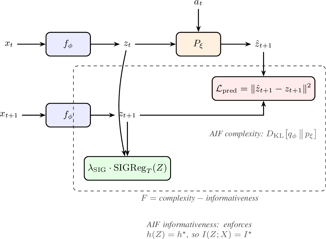
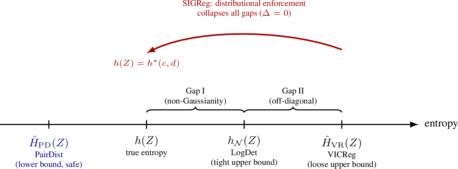
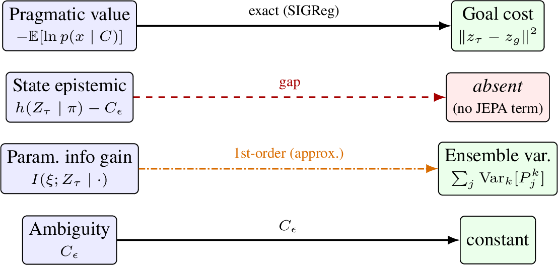
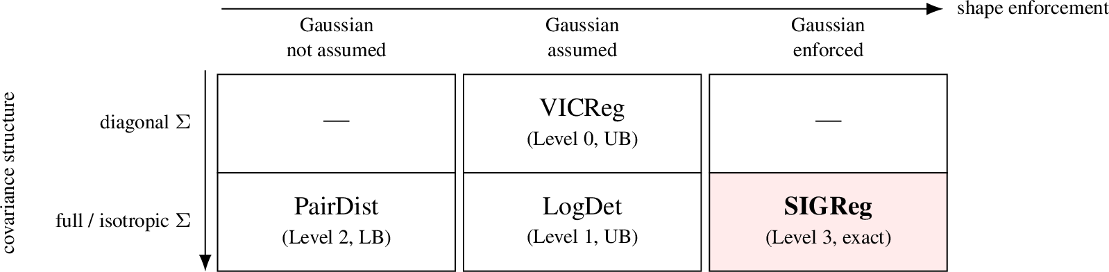
8 Positioning and Relevance↩︎
This appendix expands two points that the main text states only briefly: how the contribution differs from the closely related JEPA literature (§8.1), and why the active-inference perspective it introduces is worth having (§8.2).
8.1 Differentiation from the JEPA programme↩︎
Because the JEPA line of work is closely related and shares authorship, it is worth stating precisely how this paper differs from each prior result. The contribution is orthogonal to each, a different kind of statement about the same systems, rather than an increment on any of them.
8.1.0.1 The architecture and design programme.
The Joint-Embedding Predictive Architecture and the path-to-autonomy programme [2] are an engineering proposal: they specify how to build a latent world model that learns from observation and plans without pixel-level reconstruction, and they justify the design by what it enables. This paper supplies the normative account those designs lacked. It identifies the principle, minimisation of an Active Inference variational free energy, that a SIGReg-regularised JEPA implicitly optimises, and thereby explains why the architecture has the form it does rather than only that it works. The two are complementary: the programme provides the object, and the present theory provides its interpretation.
8.1.0.2 The regularisers.
VICReg [6] and LeJEPA/SIGReg [15] propose anti-collapse regularisers and justify them on self-supervised grounds, avoidance of representational collapse and downstream task performance. This paper evaluates the same regularisers against an external criterion: whether the implied entropy estimator preserves the Active Inference free-energy bound. That criterion, the bound type of the estimator (Proposition 2), is invisible from within the SSL framing, and it is what distinguishes SIGReg from VICReg in kind rather than degree. The hierarchy of Section 4.1 is, in effect, a reading of the regulariser landscape through a lens the original proposals did not use.
8.1.0.3 The optimum-characterising results.
The Gaussian-Embeddings result [17] shows that a successfully trained JEPA is approximately Gaussian, a property of the optimum. The linear-identifiability result [16] establishes when the trained encoder recovers the world’s latent up to a linear transform, the state-representation precondition of Section 4.6. This paper uses both differently. It uses the signed gap from exact Gaussianity (not the fact of approximate Gaussianity) to make a claim about the AIF bound and about the training path, not only the optimum; and it consumes the identifiability guarantee as an upstream precondition for a planning and control correspondence that the identifiability authors explicitly leave open. The three results triangulate the same isotropic-Gaussian target from maximum-entropy, density-estimation, and spectral-identifiability directions respectively, which is a positioning strength rather than a redundancy.
8.1.0.4 The world models and planners.
LeWorldModel [11], DINO-WM [9], PLDM [8], V-JEPA 2 [10], and the planning ablations of [19] build and benchmark JEPA world models and their planners. This paper shows that the components those systems already use (the latent goal cost, the ensemble-disagreement penalty, the model-predictive planner) are specific Active Inference quantities (Propositions 5–6): the goal cost is the pragmatic value, the ensemble disagreement is the parameter information gain, and MPC with one-step replanning realises the exact executed-trajectory correspondence. It further identifies the one AIF term none of these systems computes, the state-epistemic value, and converts the whole mapping into falsifiable predictions. In one line: the JEPA programme asks how to build world models that work; this paper asks why a particular regulariser makes them Active Inference agents, and what that implies for what they should compute.
8.2 Relevance and potential impact of the active-inference perspective↩︎
A correspondence theorem invites a fair question: granting that the mathematics holds, what does the active-inference reading actually buy? We give four answers, ordered from the most concrete to the most speculative, and flag the last two as conjectural.
8.2.0.1 A normative selection criterion for regularisers.
The most immediate consequence is practical. Absent a normative principle, the choice among anti-collapse regularisers is made on empirical grounds that do not transfer across settings. The AIF reading supplies a criterion that does transfer: a regulariser should preserve the free-energy bound, which requires a lower-bound (or exact) entropy estimator rather than an upper-bound one (Proposition 2). This both explains an existing empirical preference for SIGReg and predicts the behaviour of regularisers not yet proposed, by locating them on the two-dimensional design space of Figure 4. The criterion is useful independently of whether one accepts the full AIF framing, because it is ultimately a statement about information-theoretic safety.
8.2.0.2 A concrete, missing architectural component.
The decomposition identifies a specific term, the state-epistemic value, the entropy of the predicted future-state distribution under a policy (Proposition 6), that no current JEPA world model computes. This is not a philosophical observation but an engineering target: it names a coverage signal that, if added to the planning objective, would give a JEPA agent a principled drive to explore, of exactly the kind that distinguishes active-inference agents from purely goal-reaching controllers. The perspective thus does more than re-describe existing systems; it points at a buildable addition and predicts its effect.
8.2.0.3 A bridge that lets two literatures share results.
Establishing that JEPA world models and AIF agents optimise the same functional means that results proven in one framework become available to the other. The neuroscience and theoretical-AIF literature has developed an extensive account of exploration, precision-weighting, hierarchical generative models, and the role of the habit prior; the SSL and world-model literature has developed scalable encoders, stable training, and efficient planners. A formal correspondence is the precondition for transfer in both directions, for importing AIF’s exploration machinery into scalable world models, and for giving AIF’s normative claims a concrete, large-scale computational instantiation. The learned-policy regime (Proposition 7), which casts action selection as amortised inference, is one such transfer already visible within the paper.
8.2.0.4 A conjectural broader significance.
More speculatively, and we mark this clearly as conjecture rather than established consequence, the correspondence bears on a longstanding question about whether the Free Energy Principle, often criticised as unfalsifiable in its most general form, can be given empirical teeth in artificial systems. By tying a specific FEP-derived quantity (the surprise bound) to a measurable property of a specific class of trainable models (the embedding condition number, the latent-to-physical calibration), the present work turns a portion of the principle into something a particular experiment can confirm or refute. Whether this generalises beyond the constant-noise, isotropic-Gaussian regime studied here is open, and we do not claim that a successful test of these predictions would vindicate the Free Energy Principle as a whole. The narrower claim is that the AIF perspective, applied to JEPA world models, is productive in the scientifically meaningful sense: it generates predictions that could be wrong.
9 Lean Verification↩︎
Following the precedent of [16], we formally verify the algebraic core of this paper’s results, namely the Gaussian bridge 4 with its optimiser-set equivalence, the three-source gap decomposition and the bound-type dichotomy (Propositions 1 and 2, Corollary 2(i)), the single-step correspondence (Proposition 3, Theorem 1(i)–(iii)), the exact expected-free-energy term identities (Propositions 5 and 6; Proposition 8), the amortised-policy result (Proposition 7), and the exact parts of the multi-step correspondence (Propositions 2 and 4, Corollary 5, Theorem 2(i),(iii),(iv)), in the Lean 4 theorem prover [43] using the Mathlib mathematical library [44]. The development compiles with zero
sorry obligations: every logical step from the stated premises to the stated conclusions is machine-checked.
9.0.0.1 Scope and methodology.
Lean verification requires every inference step to be justified by a previously established lemma, hypothesis, or axiom. When a standard result exists in Mathlib (e.g.Real.log_le_sub_one_of_pos for \(\ln x\le
x-1\), ConcaveOn.le_map_sum for Jensen’s inequality), we invoke it directly. Analytic facts that Mathlib cannot yet express at our encoding, because they concern differential entropies of distributions that the scalar development treats
as opaque real parameters, enter as named hypotheses in the theorem statements rather than as global axioms: the maximum-entropy theorem behind Gap I [34], the isotropic-Gaussian entropy value behind enforcement [34], conditioning-reduces-entropy behind
Proposition 6, and the Fact-1 surprise bound. This is a deliberate refinement of the axiom-based convention of [16]: over opaque real-valued parameters a global axiom would be unsound, and the hypothesis form makes each result’s analytic dependencies auditable in its own signature. Exactly one classical
result is introduced as a Lean axiom, because it is stateable about concrete Mathlib objects and is absent from Mathlib: Hadamard’s determinant inequality for positive-semidefinite real matrices [33], consumed only by the matrix form of Gap II in Proposition 1. The complete reasoning
chains between these inputs are fully verified; Table 5 gives the inventory. One scoping rule is worth stating: the finite-sample rate (Proposition 4)
is excluded entirely, because its quantitative Cramér–Wold step is classical only in qualitative form (Remark 3), and axiomatising unsettled mathematics would counterfeit the
standard under which axioms stand for settled results; the Taylor-remainder analyses (Proposition 3, Theorem 2(ii)) are likewise deferred rather than axiomatised.
9.0.0.2 What is verified.
All reasoning between the stated inputs is machine-checked: the bridge identity, the nonnegativity of its constant \(C_{\mathrm{KL}}\), and the optimiser-set equivalence between KL and squared error; the three-source
decomposition and, from the Hadamard axiom, the sign of Gap II; the bound-type dichotomy of Proposition 2 and the exact linear slack of Corollary 2(i); Gibbs’ inequality, the KL-completion identity, and the Boltzmann-optimality of Proposition 7 in full; the teacher-forced summation of Proposition 2; the unrolled Lipschitz recurrence and the planning-MSE decomposition of
Proposition 4; the executed-trajectory specialisation of Corollary 5; the
ranking-fidelity equivalence of Theorem 2(iv); and the Jensen argument that isotropy maximises the Gaussian log-volume at fixed total variance (Proposition 3). The correspondence statements themselves (Proposition 3, Theorem 1(i)–(iii), Proposition 6, Theorem 2(i),(iii)) are verified as assemblies: their algebra is machine-checked, with successful SIGReg enforcement entering as an explicit hypothesis, matching the scoping of Remark 2. The formalisation also surfaced an additive-constant bookkeeping discrepancy between an earlier draft of Definition 3
and the per-step free energy of Appendix 6; Definition 3 as stated incorporates the correction, and the offset identity is itself a
machine-checked lemma (mainText_constant_offset).
| Result | Lean declaration | Status |
|---|---|---|
| Gaussian bridge [eq:bridge]; \(C_{\mathrm{KL}}\ge0\); argmin equiv. | gaussKL_eq, gaussKL_le_iff | verified |
| Prop. [prop:gap] decomposition; Gap II \(\le0\) | gap_decomposition, gapII_nonpos | verified\(^{\dagger}\) |
| Prop. [prop:boundtype] (bound type) | boundtype_* | verified |
| Cor. [cor:graceful](i) (linear slack) | graceful_degradation_abs | verified |
| Prop. [prop:sigzero]; isotropy maximises | sigreg_zero_gap; isotropy_maximises | assembly; verified |
| Thm. [thm:correspondence](i)–(iii) | correspondence_single_step | assembly |
| Prop. [prop:pragmatic]/[app:prop:pragmatic] (exact KL proxy) | pragmatic_exact | verified |
| Prop. [prop:o2] (state-epistemic ceiling) | state_epistemic_bound | assembly |
| Prop. [prop:policy] (KL completion; argmin) | policy_kl_completion, policy_argmin | verified |
| Prop. [app:prop:tf] (teacher-forced KL–MSE) | teacherForced_kl_mse | verified |
| Prop. [app:prop:comp] (compounding; plan-MSE decomp.) | compounding_error_bound | verified |
| Cor. [app:cor:mpc] (\(m{=}1\) exactness) | executed_trajectory_exact | verified |
| Thm. [thm:multistep](i),(iii); (iv) ranking | multistep_correspondence; ranking_fidelity | assembly; verified |
| Prop. [app:prop:efe-rest] risk identity | risk_identity | verified |
3pt
\(^{\dagger}\)
The matrix form of Gap II consumes the declared Hadamard axiom; all log algebra is machine-checked.
9.0.0.3 Build information.
The project comprises 37 Lean theorem/lemma declarations, 12 definitions, and 1 axiom across six modules (746 lines of Lean). These are Lean declarations, which do not map one-to-one onto the paper’s numbered results: Lean does not distinguish
proposition or corollary from theorem, and a single result typically expands into several declarations (one per clause), together with supporting lemmas that the prose folds away (e.g.Gibbs’ inequality behind Proposition 7, or the Boltzmann normalisation facts behind its argmin corollary). The development compiles against Lean 4 v4.32.0 with Mathlib v4.32.0 (8,662 build targets, zero errors, zero sorry
obligations). A per-theorem #print axioms audit confirms that every declaration depends only on Mathlib’s three standard axioms (propext, Classical.choice, Quot.sound), except the matrix form of Gap II,
which additionally depends on the declared Hadamard axiom. The development is publicly available at https://github.com/FabioArnez/sigreg-vfe-correspondence-lean.
References↩︎
Corresponding author; comments on this manuscript are welcome. This paper establishes a formal correspondence between the SIGReg objective and the Active Inference framework. Empirical validation of its predictions is left to separate work.↩︎