Retrieving and Integrating Historical Analogies for Foresight Analysis
July 15, 2026
1 Introduction↩︎
In the study of history, similar events are sometimes found to re-occur and hence systematic comparisons between current situations and similar histories provide us insights for foresight analysis [1]–[5]. Historical analogies, i.e., structurally similar past events, have been widely used in human history, such as policy makers [6], scientists [7], and practitioners [8]. In particular, [9] showed that structurally aligned analogies improve expert conflict predictions from 32% to 60% accuracy. Nevertheless, untrained human tend to only come up with superficial analogies instead of structural analysis [4], [10].
In the meantime, recently Large Language Models (LLMs) has emerged and demonstrated great promise in tackling complex reasoning tasks by learning from the extensive data [11]–[14]. Built upon powerful LLMs, Deep research (DR) agents that are equipped with more advanced planning capabilities and access to
external tools, can further produce in-depth, comprehensive answers to complex research tasks [15]. Recent sophisticated
DR agents can tackle expert-level question answering problems [16], search for the answer with complex constraints [17], and even do research tasks [18]. Therefore, it raises an intriguing research question:
Can
DRagents do analogical search and reasoning for foresight analysis?
In fact, early attempts with LLMs in finding analogies showed mixed results [19]–[22]. LLMs tend to struggle finding analogies from narrative stories [19], cross-domain narratives [21], analogies in the long context [20], and exhibit human-like tendencies to superficially similar events [22]. In order to answer the question, this work introduces a new task called (ADR) to LLM agents, where one aims to find historical events that align with the given target event (or the current situation) in
terms of the underlying mechanism. We construct the first ADR benchmark called ADR-bench that consists of \(15\) events, including \(10\) past events with
literature-documented historical analogies, as well as \(5\) recent events without literature documents. Through ADR-bench, we find that the state-of-the-art DR agents, including
OpenAI Deep Research [15], Gemini Deep Research [23], Qwen Deep Research [24], and MiroFlow [25] do not actively leverage the historical analogies when doing
foresight analysis. Even with historical analogies identified, the analysis is rather shallow.
We show that ADR is inherently a causal problem that the agent requires understanding the underlying hidden mechanism and factors shared across historical events and the current conditions [5]. Aligned with the observations in the literature [22], identifying analogies merely based on the surface-level similarity suffers from a non-identifiability issue and degraded foresight prediction. In addition, sufficient foresight requires sufficient coverage of the
underlying structure.
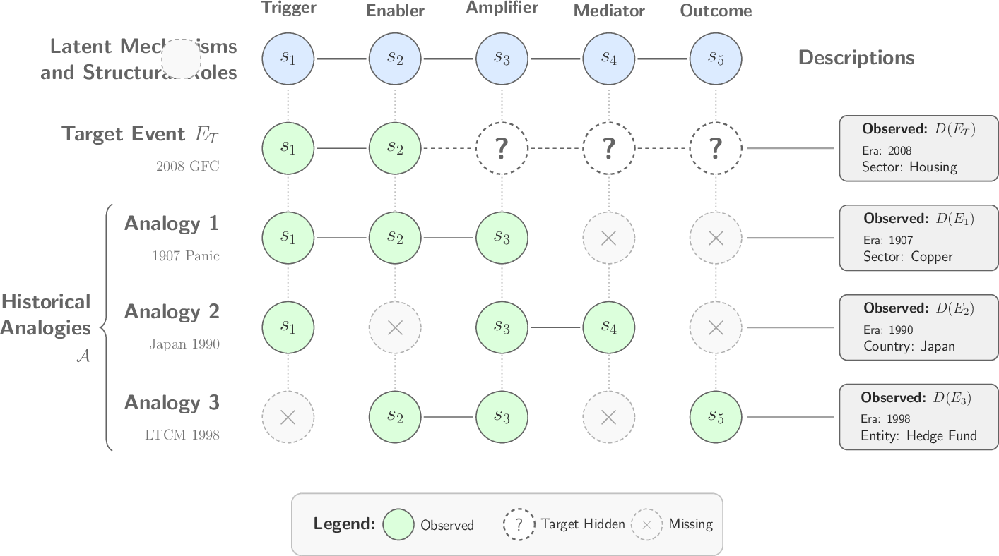
Motivated by our theoretical analysis, we propose Causal Analogical Researcher(CANA), that processes events into structural decompositions including preconditions, temporal chains, mechanisms, and outcomes.
Retrieving through the decomposed structural representation of events improves more than 10% than the state-of-the-art self-reflection method by [22].
Furthermore, we integrate the structural decomposition into the open-sourced DR agent MiroFlow, that iteratively retrieves new analogies to cover sufficient aspects of the underlying mechanisms. In ADR-bench, we show
that CANA helps identify more informative analogies, uncovering hidden driving factors, and improves the depth of foresight analysis. Our contributions can be summarized as follows:
We present the task of with the first
ADR-bench, showing the limitation of existingDRin retrieving and integrating historical analogies for foresight analysis;We present a formal framework of
ADRand show that structural representation and sufficent coverage are two principles to retrieve satisfying historical analogies;We propose the first
ADRagentCANA, that achieves more than 10% performance in historical analogy retrieval and integration than the state-of-the-art methods.
2 Related Work↩︎
Historical analogies for foresight analysis. In human history, historical analogies are widely used or cited for foresight [1]–[5]. For example, policymakers often exploit analogies to reason about the unprecedented scenarios [6], [10], [26], [27]. Scientists use analogical reasoning to identify useful hypotheses [7], [28].[9] also showed that forecasting with analogies can be largely improved from \(32\%\) to \(60\%\). Analogies refer to events that share similar mechanisms or aligned structures [29], [30]. Structural alignment of analogies helps with foresight analysis [31], which is inherently a causal problem where separate partial observations are aligned to recover the underlying causal relations [32]–[34]. We exploit the conceptual connection between analogy identification and causal learning to build our framework.
Analogical reasoning with LLMs. Due to the usefulness of analogies, there is a growing body of works trying to use LLMs to do analogical reasoning [35]. [36] showed LLMs can abstract concepts and perform analogical reasoning. [37] found that self-generated analogous examples help improve LLM reasoning. [38] showed that relating analogical sub-problems helps solve a challenging composite problem with LLMs. As LLMs are trained on extensive datasets, finding analogies with LLMs is also of great interests [19], [21], [22], [39]. [19] found that LLMs are relatively limited in finding analogies from stories. [21] also showed the limitations of LLMs in finding cross-domain analogies. [20] provided evidence on the limitations of LLMs in finding analogies in the long context. The most relevant work to ours is [22], which introduced the historical-analogy benchmark and showed that reflecting on the topics, background, process, and result can improve the historical analogy capabilities of LLMs. Nevertheless, none of the existing works fully define the problem and the principles required for historical analogy identification and integration.
Deep research and forecasting with LLMs. Deep research (DR) agent is a systematic framework to equip LLMs with advanced capabilities such as planning and tool use [40], in order to tackle complex real-world problems that require multi-step planning and reasoning [15], [41]. For example, [25], [41] showed that synthesis of comprehensive search results help tackle challenging reasoning tasks [16], [17], [42]
and even future prediction [43]. In particular, forecasting is inherently a challenging task that requires gather substantive
information [44] while of great downstream application value [45]–[47]. Despite the importance of historical analogies, we found that DR
agents do not proactively exploit the use of historical analogies by the first ADR-bench, and propose a new ADR agent to tackle the limitation.
3 Foresight with Historical Analogies↩︎
In this section, we formally define the problem of , along with its objectives and principles to realize ADR.
3.1 Problem Definition↩︎
We begin by establishing necessary concepts, and full details of the theoretical framework can be found in Appendix 9.
Definition 1 (Event Representation). An event \(E\) has two representations: (i) descriptive \(D(E) \in \mathbb{R}^p\), capturing observable surface features (entities, domain, timeline); and (ii) mechanistic \(M(E) = (V_E, \mathcal{E}_E)\), where \(V_E = \{v_1, \ldots, v_k\}\) are causal factors, \(G_E = (V_E, \mathcal{E}_E)\) is a directed graph encoding causal relationships. Depending on the event-specific context \(\chi_E\), the same \(M(E)\) can have different instantiations at the descriptive level \(D(E) = h(M(E), \chi_E)\).
Given a target event \(E_T\), we aim to find an aligned source event \(E_S\) where they share a set of structural positions \(\{s_1, \ldots, s_L\}\) in the underlying causal graphs describing the mechanisms of \(E_S\) and \(E_T\). Positions are not pre-specified but discovered through cross-event alignment [29]. Shown as in Fig. 1, roles can be assigned to the objects depending on the relational structure in the event [48].
Partial observability. Usually, the target event describes the current situation, and one can only observe part of the underlying objects \(V^{\mathrm{obs}} \subseteq V_{E_T}\) as well as the structural positions \(\mathcal{S}_T^{\mathrm{obs}} = \psi_{E_T}(V^{\mathrm{obs}})\) until the current time, or cutoff time \(t_c\), where \(\psi_{E_T}(\cdot)\) is a structural mapping that maps underlying objects in \(V_{E_T}\) to the corresponding structural roles. In addition, the remaining objects are hidden \(\mathcal{V}_T^{\mathrm{hid}} = V_{E_T} \setminus V^{\mathrm{obs}}\) occupying the hidden positions \(\mathcal{S}_T^{\mathrm{hid}} = \psi_{E_T}(V_{E_T}) \setminus \mathcal{S}_T^{\mathrm{obs}}\).
. ADR for foresight analysis requires one to find sufficient analogies in the history and align the underlying structural positions to make predictions about future trajectories.
Definition 2 (Foresight Risk with Analogies). Let \(Y_F = \Gamma(\{\tau_s(t) : s \in \mathcal{S}_T, t > t_c\})\) denote the foresight target, where \(\tau_s(t)\) describes the future trajectories of \(s\) at time \(t\), let \(P_F^w\) denote the true distribution and \(\widehat{P}_F^{\mathcal{A}}\) denote the forecasted distribution through the analogy set \(\mathcal{A}\). Then the foresight risk is \(\mathcal{R}(\mathcal{A}, w) = \sum_{s \in \mathcal{S}_T} \mu_s \cdot \mathrm{TV}(\widehat{P}_s^{\mathcal{A}}, P_s^w)\) where \(\mathrm{TV}(\cdot,\cdot)\) measures the distance between two input distributions, \(\mu_s \geq 0\), \(\sum_s \mu_s = 1\), and \(P_s^w\) is the true trajectory distribution at position \(s\).
Intuitively, let \(\mathcal{U}\) denote the universe of events, the ADR problem is to select \(\mathcal{A}^* \subseteq \mathcal{U}\) and produce foresight report consisting of uncovered
hidden factors, mechanisms, predicted trajectories, conditional scenarios, and key uncertainties. The success of ADR relies on the following assumption.
Assumption 1 (Mechanism Transfer). If factors \(v_S \in V_{E_S}\) and \(v_T \in V_{E_T}\) occupy the same structural position (\(\psi_{E_S}(v_S) = \psi_{E_T}(v_T) = s\)), both are active at their respective cutoffs, and \(E_S\) has progressed beyond \(E_T\)’s current stage, then \(\mathrm{TV}(\widehat{P}_s^{E_S}, P_s^T) \leq \alpha_s\) for some \(\alpha_s > 0\).
Assumption 1 is at the core of the literature of applied history, where people widely use historical analogies for foresight analysis [5].
3.2 Benchmark↩︎
After defining the goal of ADR, we can explore whether the state-of-the-art DR agents are able to find useful historical analogies for foresight analysis. We begin by constructing the first ADR benchmark
ADR-bench with the aim of providing insights on the performance of existing DR agents.
Event corpus. Essentially, we need events where both historical analogies are available and the foresight quality can be verified. However, one can hardly find events that jointly satisfy all the criteria. Hence, we incorporate two types of events: 10 historical events that are widely studied in the literature, and \(5\) forward events covering currently unfolding situations. The \(15\) events span financial (\(5\)), geopolitical (\(6\)), and technology (\(4\)) domains.
Per-event annotation and task design. Each event is annotated with: (1) temporal cutoff with rationale; (2) pre-cutoff analyst’s brief; (3) causal structure: including preconditions, causal chain, mechanism, outcome, and structural pattern. For forward events, we only have the approximated mechanism and current outcome since they are unfolding); (4) oracle analogies with consensus levels and documented shared mechanisms for historical events; (5) cross-analogy invariants with mechanisms that recur across the oracle analogies; and (6) hidden factors with foreseeability. We focus on foresight analysis: given only the pre-cutoff brief, produce a forward-looking analysis. The task asks the agent to “assess the underlying dynamics, evaluate the risks, and provide your forward-looking view,” without mentioning analogies, historical parallels, or hidden factors. If an agent uses analogies, it is because its architecture drives it to do so.
Evaluation design. We use a rubric-based evaluation protocol. Detailed instructions for evaluation can be found in Appendix 10. Specifically, we will extract 5-level claims, including (L1) surface fact, (L2) single-analogy insight, (L3-D) cross-analogy pattern without structural role, (L3-S) cross-analogy pattern with causal role specified and L4 hidden factor inferred from cross-analogy evidence from \(\geq\)2 events. We also report the hit rate of hidden factors. We also score analysis quality (RAS), the depth of foresight analysis (FQS), and the mechanism grounding quality (Gr).
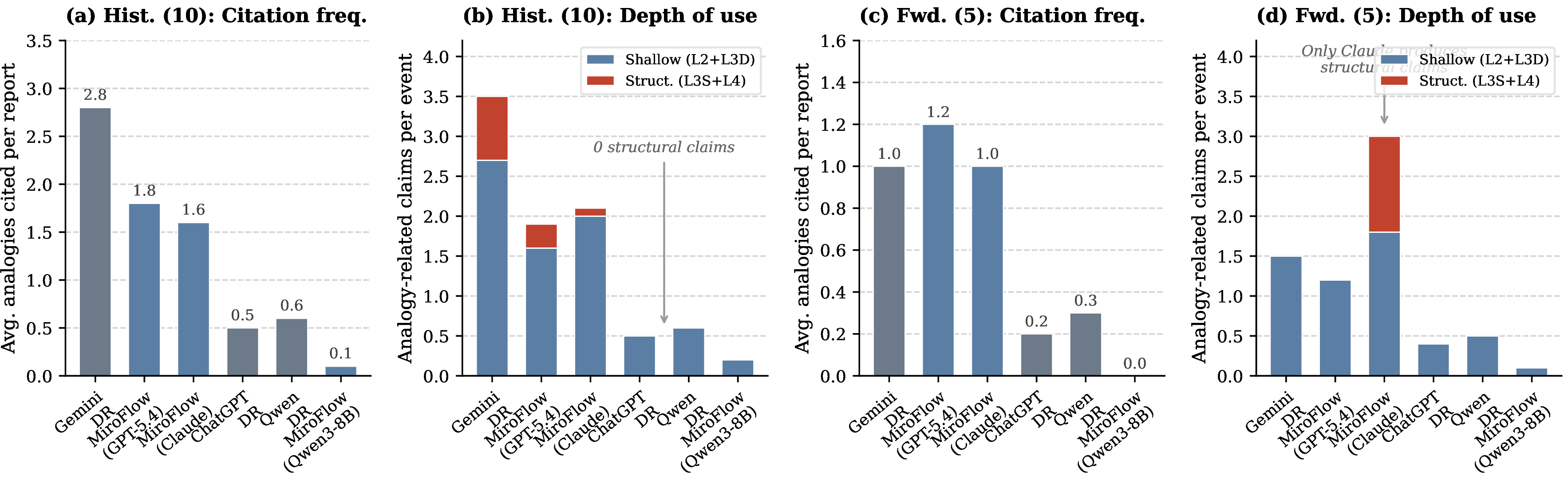
Preliminary results. We evaluate four commercial DR agents on all \(15\) events using the natural prompt: OpenAI Deep Research [15], Gemini Deep Research [23], Qwen Deep Research [24], and MiroFlow [25] with three backbone LLMs (Claude Sonnet 4.5 [49], GPT-5.4 [50], and Qwen3-8B [51]). The results are given in Fig. 2, where one can find that most of existing DR agents fail to find
useful analogies in foresight analysis. The relatively most capable agent Gemini Deep Research, can find limited analogies, but fail to produce in-depth analysis by effectively leveraging the analogies.
3.3 Theoretical Discussions↩︎
To understand why existing DR agents fail to identify useful analogies to perform foresight analysis, we provide the following theoretical discussions. To begin with, most existing DR agents are trained on planning and
synthesis queries and results at the surface-level descriptions [52], while finding historical analogies require structural alignment of the
underlying objects, roles and mechanisms.
Theorem 1 (Surface Non-Identifiability). Suppose there exist two admissible worlds \(w^0, w^1\) with identical surface observations \(\mathcal{O}_D^{\infty}(w^0) = \mathcal{O}_D^{\infty}(w^1)\), but for a hidden position \(s\), \(Z_s(w^0) \neq Z_s(w^1)\) where \(Z_s(w) = \mathbb{1}[s \in \mathcal{S}_T^{\mathrm{true}}(w)]\) that \(s\) does not align between \(w^0\) and \(w^1\), Then, no surface-level method can identify whether \(s\) is active: \(\inf_{\hat{Z}_s} \max_{j} \Pr_{w^j}(\hat{Z}_s \neq Z_s(w^j)) \geq 1/2\). If the two worlds imply separated foresight distributions \(\mathrm{TV}(P_F^{w^0}, P_F^{w^1}) \geq 2\Delta_s\), then any surface-level forecast satisfies \(\max_j \mathrm{TV}(\widehat{P}_F, P_F^{w^j}) \geq \Delta_s\). This holds for any number of analogies retrieved.
The full statement and the proof of Theorem 1 is given in Appendix 9. Intuitively, Theorem 1 implies that aligning analogies for foresight analysis requires aligning the underlying structural roles instead of the surface-level descriptions. It also explains why it is widely observed in the literature that LLMs are struggling with finding the analogies [21], [22].
Nevertheless, given the partial observability of both the target events and the potential source events, for \(K\) retrieved analogies, we may only align a few positions, which may suffer from misalignment issues, since multiple events may coincidentally align with each other.
Theorem 2 (Cross-Analogy Confirmation). Let \(X_{k,s} = \mathbb{1}[\text{analogy } E_k \text{ confirms position } s]\) with \(P(X_{k,s}=1 \mid Z_s=1) = q_{k,s}\) and \(P(X_{k,s}=1 \mid Z_s=0) = p_{k,s}\), conditionally independent across \(k\) given \(Z_s\), then \(\log \frac{P(Z_s = 1 \mid X_{\mathcal{A}})}{P(Z_s = 0 \mid X_{\mathcal{A}})} = \log\frac{\pi_s}{1-\pi_s} + \sum_{k \in \mathcal{A}} \left[ X_{k,s} \log\frac{q_{k,s}}{p_{k,s}} + (1-X_{k,s}) \log\frac{1-q_{k,s}}{1-p_{k,s}} \right],\) where \(\pi_s = P(Z_s = 1)\) is the prior probability that position \(s\) is active before observing any analogical evidence. Each independent confirming analogy multiplies posterior odds by \(q_{k,s}/p_{k,s}\), so coincidence probability decays exponentially.
The full statement and proof of Theorem 2 are given in Appendix 9. Theorem 2 states the conditions in order to sufficiently align the structures between the target events and the analogies. For example, given \(\pi_s{=}0.5, q_s{=}1, p_s{=}0.2, \delta{=}0.05\), one requires 2 independent analogies per position to distinguish the structural necessity.
Discussions with existing causal identifiability theory. As ADR is essentially a causal problem, one could also draw analogical relations between our theoretical results and the causal identifiability theories. For example,
Theorem 2 parallels the positive results from causal discovery on multiple datasets [32] and from multi-view causal representation learning [34], [53] where multiple partial views of shared latent structure enable identification of the underlying causal structure.
Design implications. One could draw practical implications from the two theoretical results as well. Specifically, we can derive two principles: Principle 1 (Theorem 1): analogy retrieval should operate on \(M(E)\) rather than \(D(E)\), since surface observations collapse mechanism-distinct worlds; and Principle 2 (Theorem 2): cross-analogy confirmation with \(K_s^* \geq 2\) independent analogies per position is needed to distinguish structural necessity from coincidence.
4 Agent↩︎
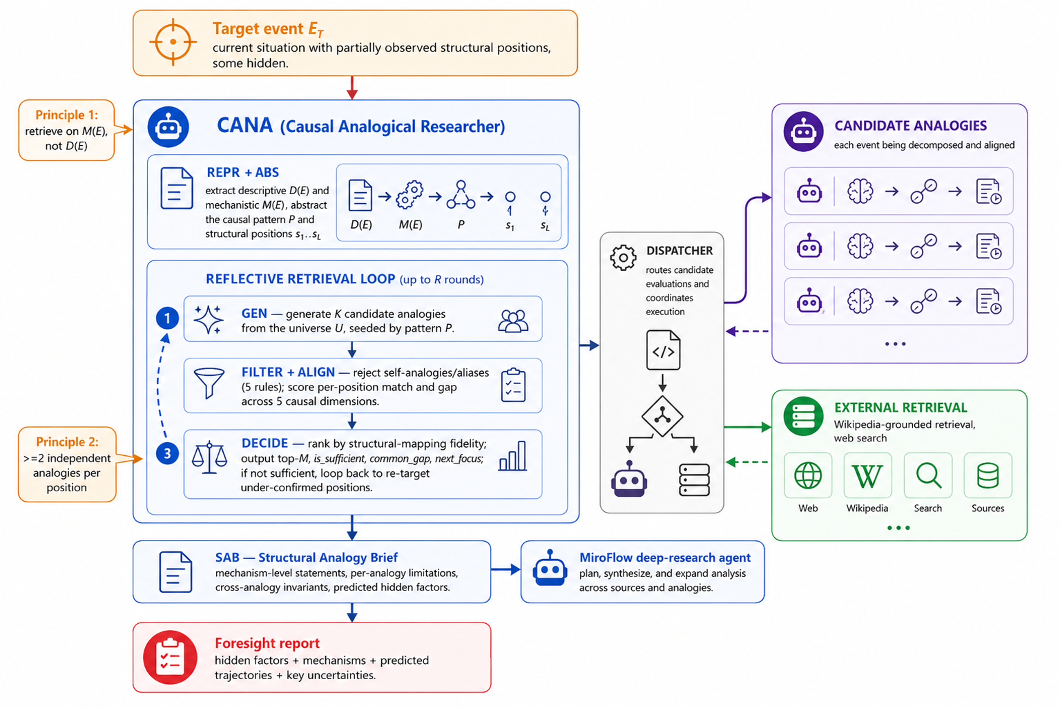
Built upon discussions in Sec. 3, we propose Causal Analogical Researcher(CANA) to realize the two principles, via (i) structural decomposed representation; and (ii)
structural reflective generation. An overview of CANA is illustrated in Fig. 3.
4.1 Causal Analogical Researcher↩︎
Structural decomposed representation. Motivated by [54], we aim to seek a general decomposed
representation of historical events, such that the follow-up structural alignment is easier. Therefore, we propose to leverage LLMs to recognize the temporal roles of events, including preconditions, temporal chains, mechanisms, and outcomes.
As mentioned in Def. 3.1 that, the positions is not unique, one may assign different roles to the objects in an event, depending on the objective and the context (e.g., the trigger–enabler–amplifier–mediator–outcome
form in Fig. 1). Since events usually unfold in a temporal order [5], we find that our
decomposition is empirically general and useful. Detailed prompts are given in Appendix 11.1.
Structural reflective generation. Following [22] that uses parametric knowledge to retrieve historical analogies, we feed structurally decomposed target events to LLMs and ask the LLM to come up with relative analogies. To realize the second principle, we also construct feedback signals to prompt the LLM to iteratively reflect and self-improve upon the generation results. Following the insights given by Theorem 2, we prompt LLMs to self-critique and reflect based on the covered and not covered aspects of the target events. After a few rounds, one could observe more cross-confirmed events and find the desired historical analogies.
Although [22] also proposed a decomposition of events and leveraged reflective signals to improve the analogy retrieval, the lack of theoretical foundations and principles make the generated results remain focused on surface features, as we will show in the experiments.
4.2 Agentic Modules for Deep Research↩︎
With the CANA developed for effective historical analogy generation, we further incorporate CANA as a lightweight module in the state-of-the-art open-source DR framework MiroFlow [25].
CANA synthesizes the Structural Analogy Brief (SAB) as additional context to the main agent DR multi-agent framework. The construction of SAB relies on the CANA decomposition. A critical
difference from previous structural reflective generation is that, SAB is designed find a more diverse set of analogies in order to cover a broad domain of possible analogies, and then do composition. Specifically, the SAB
provides mechanism-level statements, limitations of each retrieved analogy, cross-analogy insights as well as predicted hidden factors. The rich context provides grounds for DR.
| Method | T\(_{Abs}\) | T\(_{Lit}\) | T\(_{All}\) | B\(_{Abs}\) | B\(_{Lit}\) | B\(_{All}\) | P\(_{Abs}\) | P\(_{Lit}\) | P\(_{All}\) | R\(_{Abs}\) | R\(_{Lit}\) | R\(_{All}\) | MDS |
|---|---|---|---|---|---|---|---|---|---|---|---|---|---|
| gpt-5.4-mini | |||||||||||||
| 1-13 Direct Gen. | 2.24 | 0.14 | 0.46 | 2.36 | 0.11 | 0.53 | 2.38 | 0.09 | 0.60 | 2.32 | 0.10 | 0.55 | 3.05 |
| Summarizing | 2.99 | 0.18 | 0.51 | 3.03 | 0.12 | 0.67 | 3.03 | 0.11 | 0.69 | 2.95 | 0.13 | 0.64 | 3.59 |
| Self-reflection | 2.70 | 0.23 | 0.45 | 3.00 | 0.18 | 0.59 | 3.00 | 0.15 | 0.66 | 2.78 | 0.17 | 0.60 | 3.34 |
| 3.13 | 0.14 | 0.63 | 2.98 | 0.11 | 0.71 | 3.10 | 0.09 | 0.79 | 2.95 | 0.10 | 0.70 | 4.01 | |
| 1-13 | |||||||||||||
| 1-13 Direct Gen. | 1.46 | 0.19 | 0.29 | 2.23 | 0.15 | 0.42 | 2.12 | 0.14 | 0.43 | 2.21 | 0.14 | 0.41 | 2.24 |
| Summarizing | 3.16 | 0.16 | 0.59 | 3.00 | 0.10 | 0.72 | 3.08 | 0.10 | 0.76 | 3.06 | 0.11 | 0.70 | 3.91 |
| Self-reflection | 3.36 | 0.15 | 0.65 | 3.04 | 0.10 | 0.73 | 3.09 | 0.09 | 0.78 | 3.10 | 0.10 | 0.75 | 4.11 |
| 3.16 | 0.13 | 0.69 | 2.93 | 0.09 | 0.75 | 3.02 | 0.08 | 0.79 | 2.96 | 0.10 | 0.74 | 4.17 | |
| 1-13 | |||||||||||||
| 1-13 Direct Gen. | 1.00 | 0.05 | 0.30 | 1.09 | 0.05 | 0.32 | 1.11 | 0.05 | 0.33 | 1.09 | 0.05 | 0.32 | 1.76 |
| Summarizing | 2.71 | 0.17 | 0.53 | 2.76 | 0.12 | 0.63 | 2.68 | 0.11 | 0.66 | 2.69 | 0.12 | 0.62 | 3.47 |
| Self-reflection | 3.06 | 0.15 | 0.61 | 2.96 | 0.10 | 0.70 | 3.03 | 0.09 | 0.77 | 3.02 | 0.10 | 0.70 | 3.94 |
| 3.03 | 0.12 | 0.68 | 2.82 | 0.08 | 0.74 | 2.80 | 0.08 | 0.76 | 2.91 | 0.09 | 0.75 | 4.11 | |
| Method | ||||||||||
| Isom. | ||||||||||
| Con. | ||||||||||
| Con. | ||||||||||
| Suf. | ||||||||||
| Cov. | ||||||||||
| Alig. | ||||||||||
| Sim. | ||||||||||
| B. | Final | |||||||||
| gpt-5.4-mini | ||||||||||
| Direct Gen. | 1.46 | 1.77 | 1.68 | 1.84 | 0.96 | 0.95 | 2.07 | 2.02 | -0.69 | 3.31 |
| Summarizing | 1.96 | 2.16 | 2.26 | 2.75 | 1.52 | 1.79 | 1.47 | 2.77 | -0.65 | 4.49 |
| Self-reflection | 1.94 | 2.10 | 2.23 | 2.64 | 1.57 | 1.88 | 1.18 | 2.77 | -0.58 | 4.12 |
| 1.95 | 2.14 | 2.20 | 2.77 | 1.54 | 1.78 | 1.84 | 2.64 | -0.57 | 5.22 | |
| sonnet-4-6 | ||||||||||
| Direct Gen. | 1.69 | 2.07 | 1.96 | 2.07 | 1.29 | 1.48 | 2.99 | 2.19 | -0.46 | 3.43 |
| Summarizing | 1.89 | 2.05 | 2.21 | 2.66 | 1.41 | 1.68 | 1.58 | 2.71 | -0.67 | 4.65 |
| Self-reflection | 1.97 | 2.15 | 2.24 | 2.74 | 1.50 | 1.88 | 1.73 | 2.73 | -0.56 | 5.23 |
| 1.98 | 2.11 | 2.21 | 2.84 | 1.52 | 1.91 | 1.89 | 2.62 | -0.47 | 5.70 | |
| qwen3-8b | ||||||||||
| Direct Gen. | 0.855 | 1.18 | 0.59 | 0.26 | 0.11 | 0.10 | 2.94 | 0.36 | -0.17 | 2.14 |
| Summarizing | 1.88 | 2.08 | 2.11 | 2.53 | 1.39 | 1.64 | 1.79 | 2.64 | -0.66 | 4.37 |
| Self-reflection | 1.87 | 2.04 | 2.11 | 2.66 | 1.43 | 1.66 | 1.73 | 2.69 | -0.68 | 4.63 |
| 1.77 | 1.94 | 1.98 | 2.66 | 1.34 | 1.49 | 2.06 | 2.54 | -0.70 | 4.87 | |
5 Experiments↩︎
We conduct experiments using both benchmarks from [22] as well as ADR-bench, in order to verify the effectiveness of CANA
in analogy generation, and in ADR task, respectively.
5.1 Historical Analogy Generation↩︎
Setup. We used more updated LLMs ranging in different capabilities, including Qwen3-8B [51],
GPT-5.4-mini [55], and Claude-Sonnet-4.6 [56]. We compare the state-of-the-art methods proposed by [22] (i.e.,
self-reflection), direct generation, and summary-then-generation.
Evaluation. We consider two sets of evaluation protocols, one is the topic-background-process-result (MDS) decomposition by [22],
and the other is motivated by CANA decomposition, where we consider more dimensions involving the historical analogy alignment, including chain isomorphism, direction consistency, mapping consistency, overlap sufficiency, idiosyncrasy
coverage, system alignment, novelty, surface similarity, and calibration bonus. Detailed rubrics for evaluating the 9-dimension are given in Appendix 12.
Results. Results using [22] and our 9-item finegrained evaluation are given in Table 1, Table 2, respectively. We can find that, although self-reflection by [22] uses a more aligned decomposition as MDS evaluation
protocol, CANA still achieves the best performance across all LLMs. Interestingly, GPT-5.4-mini can achieve better results than self-reflection when using summary-then-generation.
Moreover, one could also notice that when using the relatively powerful LLM like Claude-Sonnet-4.6, MDS scores saturate to around \(4.1\) to \(4.2\). That is because the
decomposition of MDS does not sufficiently align with the underlying structural form of the events. In contrast, the fine-grained 9-dimension decomposition in Table 2 provides a better lens to understanding the differences
of methods. Although CANA does not use a similar fine-grained decomposition, surprisingly, CANA achieves up to 25% improvements than self-reflection when using GPT-5.4-mini. In addition, the weakest
Qwen3-8B using CANA can surpass GPT-5.4-mini with self-reflection, or Claude-Sonnet-4.6 with summarization, implying the effectiveness and generality of CANA.
Case studies. Concretely, in Table 5 in Appendix 12.1, we present examples showing the seven systematic failure modes of descriptive matching via MDS decomposition,
each resolved by CANA decomposition. It also echoes the importance of alignment via \(M(E)\) as predicted by our theory.
5.2 Evaluation↩︎
Setup. We evaluate \(10\) agent configurations on all \(15\) ADR-bench events: \(3\) commercial DR agents
(OpenAI Deep Research [15], Gemini Deep Research [23], Qwen Deep Research [24]); \(3\) vanilla MiroFlow agents [25] with
Claude Sonnet 4.5 [49], GPT-5.4 [50], and Qwen3-8B [51]; and \(3\)
CANA agents with the same three backbones. All agents receive the identical prompts as given by ADR-bench. Scoring uses the rubric-based evaluation with Claude Sonnet 4.5. We report the evaluation metrics as
introduced in Sec. 3.2.
| Historical events (10) | Forward events (5) | |||||||||||
|---|---|---|---|---|---|---|---|---|---|---|---|---|
| 3-7 (lr)9-13 | Agent | L3S+L4 | HF@L4 | RAS | FQS\(_d\) | Gr% | L3S+L4 | HF@L4 | RAS | FQS\(_d\) | Gr% | |
| Gemini DR | 0.8 | 0/22 | 0.967 | 0.71 | 0.18 | 0.0 | 0/20 | 0.889 | 0.79 | 0.21 | ||
| ChatGPT DR | 0.0 | 0/22 | 0.741 | 0.53 | 0.13 | 0.0 | 0/20 | 0.630 | 0.47 | 0.07 | ||
| Qwen DR | 0.0 | 0/22 | 0.689 | 0.37 | 0.15 | 0.0 | 0/20 | 0.600 | 0.27 | 0.08 | ||
| (GPT-5.4) | 0.3 | 1/22 | 0.933 | 0.73 | 0.34 | 0.0 | 0/20 | 0.837 | 0.86 | 0.42 | ||
| (Sonnet-4.5) | 0.1 | 0/22 | 0.819 | 0.82 | 0.35 | 1.2 | 1/20 | 0.800 | 0.55 | 0.12 | ||
| (Qwen3-8B) | 0.0 | 0/22 | 0.319 | 0.29 | 0.07 | 0.0 | 0/20 | 0.570 | 0.00 | 0.00 | ||
| (Sonnet-4.5) | 14.0 | 13/22 | 1.000 | 0.77 | 0.74 | 16.6 | 3/20 | 1.000 | 0.56 | 0.84 | ||
| (GPT-5.4) | 11.6 | 7/22 | 0.993 | 0.92 | 0.94 | 13.4 | 3/20 | 1.000 | 0.86 | 0.94 | ||
| (Qwen3-8B) | 3.2 | 1/22 | 0.607 | 0.82 | 0.81 | 6.0 | 3/20 | 0.807 | 0.62 | 0.81 | ||
4.5pt
Table 3 shows the main results across all \(15\) events. From the results, we can find that
Finding 1: DR agents are struggling in foresight analysis with historical analogies. Complementary to previous preliminary results, we can find that most DR agents fail to write in-depth foresight analysis, and
the reports given by DR agents lack of grounding mechanisms.
Finding 2: CANA improves significantly for ADR. No matter which backbone LLM is used, one could find that MiroFlow equipped with CANA show great improvements than both previous
commercial DR agents, as well as MiroFlow agents without CANA. Even using the weakest LLM Qwen3-8B, MiroFlow with CANA achieves commercial DR agent level performance
and even surpasses.
Finding 3: Complementary strengths across backbones. Different LLMs with CANA show different characteristics. Interestingly, CANA with Sonnet-4.5 comes up with substantial volume of claims (\(223\) L3-S+L4) and hidden-factors (\(16/42\) HF@L4). CANA with GPT-5.4 focuses on high-level mechanism grounding synthesis, as well as most in-depth foresight quality.
Both achieve RAS \(= 1.00\). This suggests that the lightweight SAB with CANA provides the structural reasoning scaffold, while the backbone model determines execution quality.
Connecting to theory. The HF@L4 \(= 0/42\) result for all commercial agents validates Theorem 1: surface-level methods cannot
identify hidden structural positions regardless of model capability. The lift from SAB validates Theorem 2: cross-analogy mechanism confirmation enables hidden
factor identification and high-quality foresight analysis.
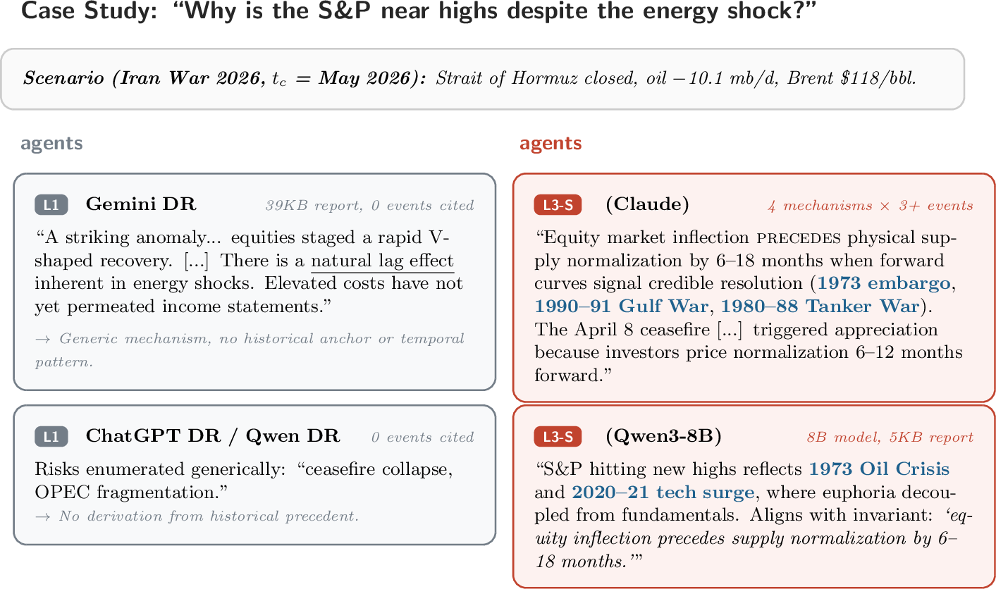
Case studies on forward event. We present a case studies of a forward event that ask agents to analyze the macro financial trends given by the Iran War 2026 and the new high of S&P 500 when the oil prices remain significantly high.
Every agent addresses this anomaly, but with dramatically different analytical depth. As shown in Fig. 4, existing DR agents cite descriptive evidence (L1), and explains that it is because of the ceasefire
effects. Nevertheless, CANA cites the historical analogies that “across 1973, 1979, 1990–91, equity inflection precedes supply normalization by 6–18 months”, which provides more in-depth reasoning underlying the
surface, aligned with the application of historical analogies by humans [5].
6 Conclusion↩︎
In this work, we introduced Analogical Deep Research (ADR) to LLM agents. We presented a theoretical framework to demonstrate the importance of identifying and aligning historical analogies for foresight analysis. By constructing the first
ADR benchmark (ADR-bench), we showed that existing DR agents lack the capability of proactively finding and leveraging historical analogies when doing foresight analysis. We derived two principles from theoretical
analysis that ADR requires structural alignment and cross-analogy confirmation, and realized the two principles via a framework called CANA. Our results show that (i) causal-inspired dimensions improve analogy retrieval by \(10\%\), (ii) CANA significantly improves the ADR on ADR-bench.
7 Related Work↩︎
Historical analogies for foresight analysis. In human history, historical analogies are widely used or cited for foresight [1]–[5]. For example, policymakers often exploit analogies to reason about unprecedented scenarios [6], [10], [26], [27]. Scientists use analogical reasoning to identify useful hypotheses [7], [28]. [9] also showed that forecasting with analogies can be largely improved from \(32\%\) to \(60\%\). Analogies refer to events that share similar mechanisms or aligned structures [29], [30]. Structural alignment of analogies helps with foresight analysis [31], which is inherently a causal problem where separate partial observations are aligned to recover the underlying causal relations [32]–[34]. We exploit the conceptual connection between analogy identification and causal learning to build our framework.
Analogical reasoning with LLMs. Due to the usefulness of analogies, there is a growing body of work using LLMs for analogical reasoning [35]. [36] showed LLMs can abstract concepts and perform analogical reasoning. [37] found that self-generated analogous examples help improve LLM reasoning. [38] showed that relating analogical sub-problems helps solve a challenging composite problem with LLMs. As LLMs are trained on extensive datasets, finding analogies with LLMs is also of great interest [19], [21], [22], [39]. [19] found that LLMs are limited in finding analogies from stories. [21] showed limitations in finding cross-domain analogies. [20] provided evidence on the limitations of LLMs in finding analogies in long contexts. The most relevant work is [22], which introduced a historical-analogy benchmark and showed that reflecting on topics, background, process, and result can improve historical analogy generation. None of these works fully define the problem and the principles required for historical analogy identification and integration.
Deep research and forecasting with LLMs. Deep research (DR) agents systematically equip LLMs with planning and tool use [40] for complex real-world problems requiring multi-step reasoning [15], [41]. For example, [25], [41] showed that synthesis of comprehensive search results helps tackle challenging reasoning tasks [16], [17], [42] and even future prediction [43]. Forecasting is inherently challenging [44] but valuable
downstream [45]–[47]. Despite the importance of historical
analogies, we find that DR agents do not proactively exploit them, and propose the first ADR agent.
LLM Use Statement↩︎
From the research side, this work studies the use of LLMs for analogical deep research. LLMs are also used to help do evaluation and experimentation. From the paper writing side, we use LLMs to assist with improving the writing of this work.
Limitation and Future Works↩︎
As a pilot work in ADR, the scale of ADR-bench might be a bit limited, and the evaluation also relies on the LLMs. Future works could scale up the curation of ADR-bench as well as more fine-grained and
human-aligned evaluation protocols.
Broader impacts↩︎
We study using LLMs for that will benefit the whole humanity and society. This work does not involve human subjects or personally identifiable information beyond public benchmarks used under their licenses.
8 Additional Technical Details↩︎
8.1 Notation↩︎
| Symbol | Meaning |
|---|---|
| \(E_T\) | Target event |
| \(\mathcal U\) | Candidate analogy universe |
| \(D(E)\) | Descriptive representation of event \(E\) |
| \(M(E)\) | Mechanistic representation of event \(E\) |
| \(\mathfrak P\) | Abstract causal pattern |
| \(\mathcal S_{\mathfrak P}\) | Structural positions in pattern \(\mathfrak P\) |
| \(\psi_E\) | Instantiation map from event factors to structural positions |
| \(\phi_k\) | Structural mapping from analogy \(E_k\) to target \(E_T\) |
| \(\Omega_{\mathrm{pos}}\) | Target-side position-level overlap |
| \(\mathcal O_D^\infty\) | Full surface observation |
| \(\mathcal O_M^\infty\) | Full mechanism-level observation |
| \(Z_s\) | Indicator that position \(s\) is truly active / structural |
| \(X_{k,s}\) | Indicator that analogy \(E_k\) confirms position \(s\) |
| \(\widehat P_s^{\mathcal A}\) | Analogy-based forecast for position \(s\) |
| \(P_s^w\) | True trajectory distribution at position \(s\) in world \(w\) |
| \(P_F^w\) | True foresight distribution in world \(w\) |
| \(\alpha_s^{\mathrm{tr}}\) | Mechanism-transfer error bound |
| \(\Delta_s\) | Position-wise two-world separation gap |
| \(\Delta_F\) | Foresight-distribution two-world separation gap |
| \(\delta_s\) | Posterior probability that inferred position \(s\) is false |
9 More Details of the Theory↩︎
9.1 Problem Definition↩︎
Definition 3 (Event Representation). An event \(E\) has two representations: (i) descriptive \(D(E) \in \mathbb{R}^p\), capturing observable surface features (entities, domain, timeline); and (ii) mechanistic \(M(E) = (V_E, G_E, \{K_{v,E}\}, \theta_E)\), where \(V_E = \{v_1, \ldots, v_k\}\) are causal factors, \(G_E = (V_E, \mathcal{E}_E)\) is a directed graph encoding causal relationships, \(K_{v,E}\) are transition kernels, and \(\theta_E\) are event-specific parameters. Each factor \(v \in V_E\) has an associated trajectory \(\tau_v: [0,T] \to \mathbb{R}\). The descriptive and mechanistic representations are related by a many-to-one mapping \(D(E) = h(M(E), \chi_E)\), where \(\chi_E\) is event-specific context.
Definition 4 (Abstract Pattern and Structural Position). An abstract causal pattern is \(\mathfrak{P} = (\mathcal{S}_{\mathfrak{P}}, G_{\mathfrak{P}})\), where \(\mathcal{S}_{\mathfrak{P}} = \{s_1, \ldots, s_L\}\) is a finite set of structural positions and \(G_{\mathfrak{P}}\) is a directed graph over \(\mathcal{S}_{\mathfrak{P}}\). Event \(E\) instantiates \(\mathfrak{P}\) via a graph homomorphism \(\psi_E: V_E \to \mathcal{S}_E \subseteq \mathcal{S}_{\mathfrak{P}}\), preserving edge structure. Factors \(v \in V_{E_1}\) and \(w \in V_{E_2}\) occupy the same structural position if \(\psi_{E_1}(v) = \psi_{E_2}(w)\). Positions are not pre-specified but discovered through cross-event alignment, following Gentner’s structure-mapping theory [29]: objects are placed in correspondence according to their roles in the common relational structure [48].
Definition 5 (Structural Mapping and Position-Level Overlap). A structural mapping from source \(E_S\) to target \(E_T\) is a partial injection \(\phi: V_{E_S} \rightharpoonup V_{E_T}\) satisfying edge preservation and position consistency: \(\psi_{E_S}(v) = \psi_{E_T}(\phi(v))\) for all \(v \in \mathrm{dom}(\phi)\). The position-level overlap for analogy set \(\mathcal{A}\) is \(\Omega_{\mathrm{pos}}(\mathcal{A}, E_T) = |\bigcup_k \psi_{E_T}(\mathrm{im}(\phi_k))| \,/\, |\mathcal{S}_T|\), measured on the target side.
Definition 7 (ADR Problem). Given target \(E_T\) at cutoff \(t_c\) with partial observation, and a universe \(\mathcal{U}\) of historical events with fully observed representations, the ADR problem is to select \(\mathcal{A}^* \subseteq \mathcal{U}\) and produce foresight report \(\mathcal{F} = (\hat{\mathcal{V}}^{\mathrm{hid}}, \hat{Y}_T, \mathcal{C}, \mathcal{K})\) maximizing: \[\mathcal{A}^* = \arg\max_{|\mathcal{A}| \leq K_{\max}} \; \mathrm{Qual}(\mathcal{F}(\mathcal{A})) - \mathrm{Qual}(\mathcal{F}(\emptyset))\] where \(\mathrm{Qual}(\mathcal{F}) = \lambda_{\mathrm{cov}} \cdot \mathrm{Cov}_{\mathrm{eval}} + \lambda_{\mathrm{prec}} \cdot \mathrm{Prec}_{\mathrm{eval}} + \lambda_{\mathrm{depth}} \cdot \mathrm{Depth}_{\mathrm{eval}}\).
Definition 8 (Surface Observation and Foresight Risk). A possible world \(w = (E_T, \mathcal{U}, \mathfrak{P}, \{\psi_E\}, t_c, \chi)\) specifies the target, analogy universe, pattern, instantiations, cutoff, and context.
For two-world comparisons, we evaluate positions on a common finite candidate universe \(\mathcal{S}_\star \subseteq \mathcal{S}_{\mathfrak P}\). For each \(s\in\mathcal{S}_\star\), define \[Z_s(w)=\mathbb{1}[s\in\mathcal{S}_T^{\mathrm{true}}(w)].\] If \(s\) is inactive in world \(w\), \(P_s^w\) denotes the corresponding null or baseline trajectory distribution.
The full surface observation is \[\mathcal{O}_D^{\infty}(w) = \left( D(E_T), \{D(E_k)\}_{E_k \in \mathcal{U}}, \{\mathrm{sim}(D(E_k), D(E_T))\}_{E_k\in\mathcal{U}} \right).\] A surface-level method is any function of \(\mathcal{O}_D^{\infty}(w)\).
The full mechanism-level observation is \[\mathcal{O}_M^\infty(w) = \left( M^{\mathrm{obs}}(E_T), \{M(E_k),\psi_{E_k},\phi_k\}_{E_k\in\mathcal{U}} \right).\] A mechanism-level method is any function of \(\mathcal{O}_M^\infty(w)\).
For a structural position \(s\), let \(\tau_s\) denote the trajectory induced by the target factor(s) \(v\in V_{E_T}\) with \(\psi_{E_T}(v)=s\), or a fixed aggregation of those trajectories when multiple factors map to \(s\). The foresight target is \[Y_F = \Gamma(\{\tau_s(t) : s \in \mathcal{S}_\star, t > t_c\})\] with true distribution \(P_F^w\) and forecast \(\widehat{P}_F^{\mathcal{A}}\).
The position-wise foresight risk is: \[\mathcal{R}(\mathcal{A}, w) = \sum_{s \in \mathcal{S}_\star} \mu_s \cdot \mathrm{TV}(\widehat{P}_s^{\mathcal{A}}, P_s^w),\] where \(\mu_s \geq 0\), \(\sum_s \mu_s = 1\).
9.2 Main Results↩︎
We state one assumption and two theorems. Theorem 3 is an information-theoretic impossibility result for surface matching; Theorem 4 quantifies the benefit of cross-analogy mechanism matching. For readability, we state the results for deterministic methods. Randomized methods satisfy the same bounds in expectation over their internal randomness.
Assumption 2 (Mechanism Transfer). If factors \(v_S \in V_{E_S}\) and \(v_T \in V_{E_T}\) occupy the same structural position (\(\psi_{E_S}(v_S) = \psi_{E_T}(v_T) = s\)), both are active at their respective cutoffs, and \(E_S\) has progressed beyond \(E_T\)’s current stage, then: \[\mathrm{TV}(\widehat{P}_s^{E_S}, P_s^T) \leq \alpha_s^{\mathrm{tr}}\] for some position-specific transfer-error bound \(\alpha_s^{\mathrm{tr}} > 0\).
Theorem 3 (Surface Non-Identifiability). Suppose there exist two admissible worlds \(w^0, w^1\) such that \(\mathcal{O}_D^{\infty}(w^0) = \mathcal{O}_D^{\infty}(w^1)\) (identical surface observations), but for a hidden position \(s\): \(Z_s(w^0) \neq Z_s(w^1)\), where \(Z_s(w) = \mathbb{1}[s \in \mathcal{S}_T^{\mathrm{true}}(w)]\). Then no surface-level method can identify whether \(s\) is active: \[\inf_{\hat{Z}_s = f(\mathcal{O}_D^{\infty})} \max_{j \in \{0,1\}} \Pr_{w^j}(\hat{Z}_s \neq Z_s(w^j)) \geq \tfrac{1}{2}\] If the two worlds imply separated foresight distributions, \(\mathrm{TV}(P_F^{w^0}, P_F^{w^1}) \geq 2\Delta_F\), then: \[\inf_{\widehat{P}_F = f(\mathcal{O}_D^{\infty})} \max_{j \in \{0,1\}} \mathrm{TV}(\widehat{P}_F, P_F^{w^j}) \geq \Delta_F\] This holds for all \(K\) including \(K = \infty\): adding more surface-matched analogies cannot eliminate foresight risk caused by \(D\)-unidentifiable hidden mechanisms.
Proof. Let a possibly randomized surface-level estimator be written as \[\hat{Z}_s=\varphi(\mathcal{O}_D^\infty,R),\] where \(R\) denotes internal randomness independent of the world. Since \[\mathcal{O}_D^\infty(w^0)=\mathcal{O}_D^\infty(w^1),\] the distribution of \(\hat{Z}_s\) is the same under \(w^0\) and \(w^1\).
Without loss of generality, suppose \[Z_s(w^0)=0, \qquad Z_s(w^1)=1.\] Let \[r=\Pr(\hat{Z}_s=1).\] Because the estimator has the same output distribution in both worlds, its error probability in world \(w^0\) is \(r\), while its error probability in world \(w^1\) is \(1-r\). Hence \[\max_{j\in\{0,1\}} \Pr_{w^j}(\hat{Z}_s\neq Z_s(w^j)) = \max\{r,1-r\} \geq \frac{1}{2}.\] Taking the infimum over all surface-level estimators gives \[\inf_{\hat{Z}_s=f(\mathcal{O}_D^\infty)} \max_{j\in\{0,1\}} \Pr_{w^j}(\hat{Z}_s\neq Z_s(w^j)) \geq \frac{1}{2}.\]
For the foresight part, let a possibly randomized forecast be \[\widehat{P}_F=\Phi(\mathcal{O}_D^\infty,R).\] Again, because the full surface observation is identical in \(w^0\) and \(w^1\), the forecast has the same distribution under both worlds. For any realization of \(R\), the triangle inequality for total variation gives \[\mathrm{TV}(P_F^{w^0},P_F^{w^1}) \leq \mathrm{TV}(P_F^{w^0},\widehat{P}_F) + \mathrm{TV}(\widehat{P}_F,P_F^{w^1}).\] Taking expectation over \(R\) if the method is randomized, we obtain \[\mathbb{E}_R\mathrm{TV}(P_F^{w^0},\widehat{P}_F) + \mathbb{E}_R\mathrm{TV}(\widehat{P}_F,P_F^{w^1}) \geq \mathrm{TV}(P_F^{w^0},P_F^{w^1}).\] Therefore, \[\max_{j\in\{0,1\}} \mathbb{E}_R\mathrm{TV}(\widehat{P}_F,P_F^{w^j}) \geq \frac{1}{2} \mathrm{TV}(P_F^{w^0},P_F^{w^1}).\] Using the assumed separation \[\mathrm{TV}(P_F^{w^0},P_F^{w^1})\geq 2\Delta_F,\] we get \[\max_{j\in\{0,1\}} \mathbb{E}_R\mathrm{TV}(\widehat{P}_F,P_F^{w^j}) \geq \Delta_F.\] For deterministic forecasts, the expectations over \(R\) disappear.
Finally, a finite-budget surface matcher with any budget \(K\) is only a measurable function of \(\mathcal{O}_D^\infty\). Since even the full surface observation is identical in the two worlds, no finite subset of surface-matched analogies can distinguish them. Thus the lower bound holds for all finite \(K\), and also when \(K=\infty\). ◻
Lemma 1 (Position-wise Surface Lower Bound). Let \(H \subseteq \mathcal{S}_\star\) be a set of candidate hidden positions. Suppose there exist two admissible worlds \(w^0,w^1\) such that \[\mathcal{O}_D^\infty(w^0)=\mathcal{O}_D^\infty(w^1),\] and for every \(s\in H\), \[\mathrm{TV}(P_s^{w^0},P_s^{w^1})\geq 2\Delta_s.\] Define the restricted position-wise risk \[\mathcal{R}_H(\mathcal{A},w) = \sum_{s\in H} \mu_s \mathrm{TV}(\widehat{P}_s^{\mathcal{A}},P_s^w).\] Then every surface-level method satisfies \[\inf_{\mathcal{A}_D} \max_{j\in\{0,1\}} \mathcal{R}_H(\mathcal{A}_D,w^j) \geq \sum_{s\in H} \mu_s\Delta_s.\]
Proof. Since \(\mathcal{O}_D^\infty(w^0)=\mathcal{O}_D^\infty(w^1)\), any surface-level method produces the same position-wise forecast in both worlds. Hence, for every \(s\in H\), \[\widehat{P}_s^{\mathcal{A}_D}(w^0) = \widehat{P}_s^{\mathcal{A}_D}(w^1) = \widehat{P}_s^{\mathcal{A}_D}.\]
By the triangle inequality for total variation, \[\mathrm{TV}(P_s^{w^0},P_s^{w^1}) \leq \mathrm{TV}(P_s^{w^0},\widehat{P}_s^{\mathcal{A}_D}) + \mathrm{TV}(\widehat{P}_s^{\mathcal{A}_D},P_s^{w^1}).\]
Using the assumed separation \[\mathrm{TV}(P_s^{w^0},P_s^{w^1})\geq 2\Delta_s,\] we obtain \[\mathrm{TV}(\widehat{P}_s^{\mathcal{A}_D},P_s^{w^0}) + \mathrm{TV}(\widehat{P}_s^{\mathcal{A}_D},P_s^{w^1}) \geq 2\Delta_s.\]
Multiplying by \(\mu_s\) and summing over \(s\in H\) gives \[\mathcal{R}_H(\mathcal{A}_D,w^0) + \mathcal{R}_H(\mathcal{A}_D,w^1) \geq 2 \sum_{s\in H} \mu_s\Delta_s.\]
Therefore, \[\max_{j\in\{0,1\}} \mathcal{R}_H(\mathcal{A}_D,w^j) \geq \frac{1}{2} \left[ \mathcal{R}_H(\mathcal{A}_D,w^0) + \mathcal{R}_H(\mathcal{A}_D,w^1) \right] \geq \sum_{s\in H} \mu_s\Delta_s.\]
Taking the infimum over all surface-level methods yields \[\inf_{\mathcal{A}_D} \max_{j\in\{0,1\}} \mathcal{R}_H(\mathcal{A}_D,w^j) \geq \sum_{s\in H} \mu_s\Delta_s.\] ◻
Corollary 1 (Mechanism Matching Breaks the Lower Bound). Let \(H\subseteq\mathcal{S}_\star\) be a set of hidden candidate positions satisfying the assumptions of Lemma 1. Suppose further that mechanism-level evidence distinguishes the two worlds: \[\mathcal{O}_M^\infty(w^0)\neq \mathcal{O}_M^\infty(w^1),\] and that mechanism matching retrieves analogies covering every \(s\in H\) with transfer error \[\mathrm{TV}(\widehat{P}_s^{\mathcal{A}_M},P_s^{w^j})\leq \alpha_s^{\mathrm{tr}}\] for all \(s\in H\) and \(j\in\{0,1\}\). Then \[\max_j \mathcal{R}_H(\mathcal{A}_M,w^j) \leq \sum_{s\in H}\mu_s\alpha_s^{\mathrm{tr}}.\] If \[\sum_{s\in H}\mu_s\alpha_s^{\mathrm{tr}} < \sum_{s\in H}\mu_s\Delta_s,\] then mechanism matching strictly dominates every surface method on hidden positions: \[\inf_{\mathcal{A}_M} \max_j \mathcal{R}_H(\mathcal{A}_M,w^j) < \inf_{\mathcal{A}_D} \max_j \mathcal{R}_H(\mathcal{A}_D,w^j).\]
Proof. By the mechanism-transfer condition, for every \(s\in H\) and every \(j\in\{0,1\}\), \[\mathrm{TV}(\widehat{P}_s^{\mathcal{A}_M},P_s^{w^j}) \leq \alpha_s^{\mathrm{tr}}.\] Therefore, \[\mathcal{R}_H(\mathcal{A}_M,w^j) = \sum_{s\in H} \mu_s \mathrm{TV}(\widehat{P}_s^{\mathcal{A}_M},P_s^{w^j}) \leq \sum_{s\in H} \mu_s \alpha_s^{\mathrm{tr}}.\] Taking the maximum over \(j\) preserves the same upper bound: \[\max_j \mathcal{R}_H(\mathcal{A}_M,w^j) \leq \sum_{s\in H} \mu_s \alpha_s^{\mathrm{tr}}.\]
By Lemma 1, every surface-level method satisfies \[\inf_{\mathcal{A}_D} \max_j \mathcal{R}_H(\mathcal{A}_D,w^j) \geq \sum_{s\in H} \mu_s \Delta_s.\] If \[\sum_{s\in H}\mu_s\alpha_s^{\mathrm{tr}} < \sum_{s\in H}\mu_s\Delta_s,\] then the mechanism-level upper bound lies strictly below the surface-level lower bound. Hence there exists a mechanism-level method whose worst-case hidden-position risk is strictly smaller than the worst-case risk of every surface-level method. ◻
Theorem 4 (Cross-Analogy Confirmation). Let \(Z_s = \mathbb{1}[s \in \mathcal{S}_T^{\mathrm{true}}]\) and \(X_{k,s} = \mathbb{1}[\text{analogy } E_k \text{ confirms position } s]\). Let \(\pi_s=P(Z_s=1)\) and \(X_{\mathcal{A},s}=\{X_{k,s}:E_k\in\mathcal{A}\}\).
Assume \(X_{k,s} \mid Z_s\) are conditionally independent with \[q_{k,s}=P(X_{k,s}=1 \mid Z_s=1,E_k\in\mathcal{A}), \qquad p_{k,s}=P(X_{k,s}=1 \mid Z_s=0,E_k\in\mathcal{A}),\] where \(q_{k,s} > p_{k,s}\). The probabilities are understood conditional on the selection rule that produced \(\mathcal{A}\).
Then: \[\log \frac{P(Z_s = 1 \mid X_{\mathcal{A},s})}{P(Z_s = 0 \mid X_{\mathcal{A},s})} = \log\frac{\pi_s}{1-\pi_s} + \sum_{E_k \in \mathcal{A}} \left[ X_{k,s} \log\frac{q_{k,s}}{p_{k,s}} + (1-X_{k,s}) \log\frac{1-q_{k,s}}{1-p_{k,s}} \right].\] The Bayes factor grows multiplicatively: each independent confirming analogy multiplies odds by \(q_{k,s}/p_{k,s}\).
In the homogeneous positive-confirmation case, \(q_{k,s}=q_s\), \(p_{k,s}=p_s\), and \(X_{k,s}=1\) for all \(E_k\in\mathcal{A}\), the number of confirmations needed to reach posterior confidence \(1-\delta\) is \[n_s^* = \left\lceil \frac{ \log\frac{1-\delta}{\delta} - \log\frac{\pi_s}{1-\pi_s} }{ \log\frac{q_s}{p_s} } \right\rceil.\] Under the calibrated regime \((\pi_s = 0.5, q_s = 1, p_s = 0.2)\), this gives \(n_s^*=2\) for \(\delta=0.05\).
For foresight, letting \[\delta_s=P(Z_s=0\mid X_{\mathcal{A},s}),\] the posterior expected risk at position \(s\) satisfies \[\mathbb{E}[\mathrm{TV}(\widehat{P}_s^{\mathcal{A}_M}, P_s^T) \mid X_{\mathcal{A},s}] \leq (1 - \delta_s)\alpha_s^{\mathrm{tr}} + \delta_s.\]
Proof. Let \[X_{\mathcal{A},s}=\{X_{k,s}:E_k\in\mathcal{A}\}.\] For a fixed realization \(x_{\mathcal{A},s}\), define the likelihood under the structural hypothesis \(Z_s=1\): \[L_1(x_{\mathcal{A},s}) = P(X_{\mathcal{A},s}=x_{\mathcal{A},s}\mid Z_s=1).\] By conditional independence, \[L_1(x_{\mathcal{A},s}) = \prod_{E_k\in\mathcal{A}} q_{k,s}^{x_{k,s}} (1-q_{k,s})^{1-x_{k,s}}.\] Similarly, under the coincidence hypothesis \(Z_s=0\), \[L_0(x_{\mathcal{A},s}) = P(X_{\mathcal{A},s}=x_{\mathcal{A},s}\mid Z_s=0) = \prod_{E_k\in\mathcal{A}} p_{k,s}^{x_{k,s}} (1-p_{k,s})^{1-x_{k,s}}.\]
By Bayes’ theorem, \[P(Z_s=1\mid X_{\mathcal{A},s}) = \frac{ \pi_s L_1(X_{\mathcal{A},s}) }{ \pi_s L_1(X_{\mathcal{A},s}) + (1-\pi_s)L_0(X_{\mathcal{A},s}) }.\] Likewise, \[P(Z_s=0\mid X_{\mathcal{A},s}) = \frac{ (1-\pi_s) L_0(X_{\mathcal{A},s}) }{ \pi_s L_1(X_{\mathcal{A},s}) + (1-\pi_s)L_0(X_{\mathcal{A},s}) }.\] Therefore the posterior odds are \[\frac{ P(Z_s=1\mid X_{\mathcal{A},s}) }{ P(Z_s=0\mid X_{\mathcal{A},s}) } = \frac{\pi_s}{1-\pi_s} \cdot \frac{L_1(X_{\mathcal{A},s})}{L_0(X_{\mathcal{A},s})}.\] The likelihood ratio is \[\frac{L_1(X_{\mathcal{A},s})}{L_0(X_{\mathcal{A},s})} = \prod_{E_k\in\mathcal{A}} \left(\frac{q_{k,s}}{p_{k,s}}\right)^{X_{k,s}} \left(\frac{1-q_{k,s}}{1-p_{k,s}}\right)^{1-X_{k,s}}.\] Taking logarithms gives \[\log \frac{P(Z_s = 1 \mid X_{\mathcal{A},s})}{P(Z_s = 0 \mid X_{\mathcal{A},s})} = \log\frac{\pi_s}{1-\pi_s} + \sum_{E_k\in \mathcal{A}} \left[ X_{k,s}\log\frac{q_{k,s}}{p_{k,s}} + (1-X_{k,s})\log\frac{1-q_{k,s}}{1-p_{k,s}} \right].\]
If \(X_{k,s}=1\) for every \(E_k\in\mathcal{A}\), then the Bayes factor reduces to \[BF_s(\mathcal{A}) = \prod_{E_k\in\mathcal{A}} \frac{q_{k,s}}{p_{k,s}}.\] Thus every independent confirming analogy multiplies the posterior odds by \(q_{k,s}/p_{k,s}\).
In the homogeneous case \(q_{k,s}=q_s\) and \(p_{k,s}=p_s\), with \(K\) positive confirmations, \[BF_s(K) = \left(\frac{q_s}{p_s}\right)^K.\] The posterior odds are \[\frac{ P(Z_s=1\mid K\text{ positives}) }{ P(Z_s=0\mid K\text{ positives}) } = \frac{\pi_s}{1-\pi_s} \left(\frac{q_s}{p_s}\right)^K.\] To achieve posterior confidence at least \(1-\delta\), we require \[\frac{\pi_s}{1-\pi_s} \left(\frac{q_s}{p_s}\right)^K \geq \frac{1-\delta}{\delta}.\] Solving for \(K\) yields \[K \geq \frac{ \log\frac{1-\delta}{\delta} - \log\frac{\pi_s}{1-\pi_s} }{ \log\frac{q_s}{p_s} }.\] Hence the minimum integer number of confirmations is \[n_s^* = \left\lceil \frac{ \log\frac{1-\delta}{\delta} - \log\frac{\pi_s}{1-\pi_s} }{ \log\frac{q_s}{p_s} } \right\rceil.\] For the calibrated regime \[\pi_s=0.5,\qquad q_s=1,\qquad p_s=0.2,\qquad \delta=0.05,\] we have prior odds equal to \(1\), and the required posterior odds are \[\frac{1-\delta}{\delta} = \frac{0.95}{0.05} = 19.\] Since \[\frac{q_s}{p_s}=5,\] one confirmation gives odds \(5<19\), while two confirmations give odds \(25>19\). Therefore \[n_s^*=2.\]
For the foresight-risk bound, define \[\delta_s = P(Z_s=0\mid X_{\mathcal{A},s}).\] With posterior probability \(1-\delta_s\), position \(s\) is truly structural. Under this event, the mechanism-transfer assumption gives \[\mathrm{TV}(\widehat{P}_s^{\mathcal{A}_M},P_s^T) \leq \alpha_s^{\mathrm{tr}}.\] With posterior probability \(\delta_s\), the inferred position is coincidental or otherwise not truly structural. In that case we use the trivial upper bound \[\mathrm{TV}(\widehat{P}_s^{\mathcal{A}_M},P_s^T) \leq 1.\] Therefore, \[\mathbb{E} \left[ \mathrm{TV}(\widehat{P}_s^{\mathcal{A}_M},P_s^T) \mid X_{\mathcal{A},s} \right] \leq (1-\delta_s)\alpha_s^{\mathrm{tr}} + \delta_s\cdot 1.\] Thus, \[\mathbb{E} \left[ \mathrm{TV}(\widehat{P}_s^{\mathcal{A}_M},P_s^T) \mid X_{\mathcal{A},s} \right] \leq (1-\delta_s)\alpha_s^{\mathrm{tr}} + \delta_s.\] This separates the two sources of foresight error: identification error \(\delta_s\) and transfer error \(\alpha_s^{\mathrm{tr}}\). ◻
10 More Details of ADR-bench↩︎
We list the rubric prompts used in ADR-bench as below.
11 More Details of CANA↩︎
11.1 CANA for historical analogy generation↩︎
The algorithmic description of CANA used for
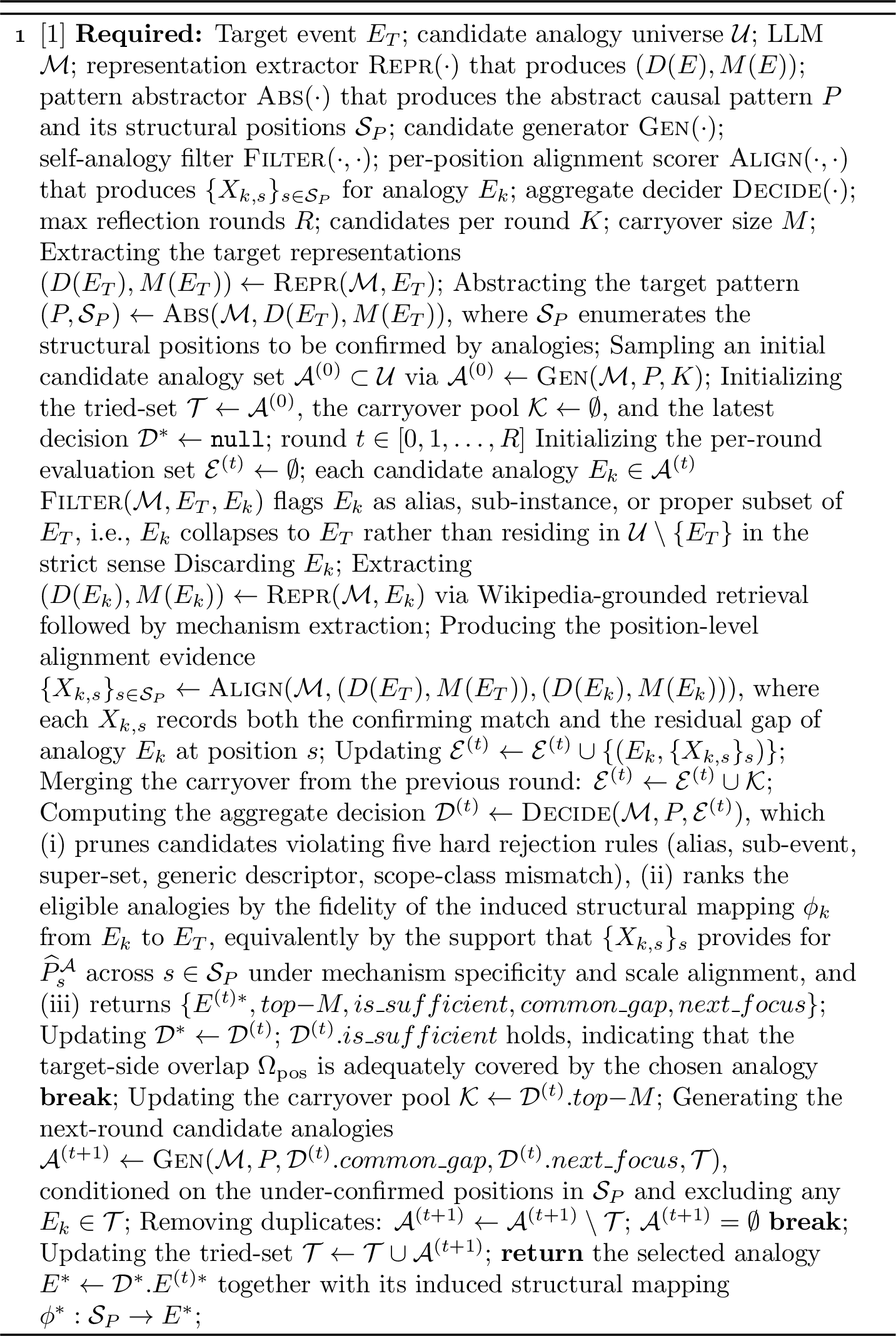
We present the prompts we used in CANA:
12 Rubric-based Evaluation for Historical Analogy Generation↩︎
We provide our new evaluation protocols for [22].
Seven failure modes resolved. Concretely, in Table 5, we present examples showing the seven systematic failure modes of descriptive matching via MDS decomposition, each resolved by CANA
decomposition. It also echoes the importance of alignment via \(M(E)\) as predicted by our theory.
12.1 Failure modes of descriptive matching↩︎
| Failure Mode | Descriptive Match [22] | decomposition |
|---|---|---|
| Part-whole confusion | Arab Spring \(\to\) Tunisian Rev. | \(\to\) 1989 E.Europe |
| Same-war echo | Expedition of 1000 \(\to\) Volturno | \(\to\) Cuban Revolution |
| Self-analogy | Iraq War \(\to\) 2003 Invasion | \(\to\) Soviet-Afghan War |
| Causal direction error | Battle of Bulge \(\to\) Market Garden | \(\to\) Michael Offensive |
| Surface feature match | Caesar \(\to\) Lincoln | \(\to\) Cromwell’s death |
| Proximity bias | J.Brown’s Raid \(\to\) Bleeding Kansas | \(\to\) Easter Rising |
| Domain closure | Canudos \(\to\) Siege of Balaler | \(\to\) Satsuma Rebellion |