Abstract. We develop a convergent scheme to train neural networks involving analytic activation functions based on gradient flows. Convergence properties are guaranteed by Lojasiewicz theory. The main advantage of this approach is its simplicity of implementation. The coefficients of the network are approximated by solving a system of ordinary differential equations. We test the method by constructing residual neural network approximations of solutions of parametric problems. The dependence of the solutions of simple ordinary differential equations on a few parameters is correctly reproduced. The solutions of inverse problems involving wave constraints which depend on a few parameters can be reasonably approximated, even in regions in which the problem is severely ill posed.
Keywords. Residual neural networks, approximation theory, parametric problems, differential equations, inverse problems.
MSCcodes. 68Q32, 65D15, 65K10.

1 Introduction↩︎

A wide variety of problems in applied sciences require solving large amounts of parameter-dependent ordinary or partial differential equations. For instance, technological designs often rely on large scale simulations [1]–[3] to test the response to variations of relevant parameters. Likewise, optimization and Bayesian approaches to inverse problems typically involve solving differential constraints for huge amounts of parameter proposals [4]–[6]. Sometimes, the full solution is not really needed for these applications, quantities of interest calculated from them are used in practice instead.

Over the years, a broad range of numerical schemes have been developed to approximate the solutions of models formulated in terms of differential equations with a controlled error [7], [8]. The increase in computer speed, combined with high performance computing tools, allows us to handle a growing variety of complex problems employing these methods for given parameter choices [1]–[3]. Whenever we vary a parameter, we must face the computational cost of solving the problem again. In that respect, the development of approximation procedures which are able to provide reasonable solutions for multiple parameter choices at low cost would constitute an important breakthrough. Machine learning techniques, in particular neural network (NN) based approximations [9], have raised some expectations in that respect. We will consider here their potential for the approximation of solutions of multi-parametric problems and inverse problems.

Universal approximation theorems establish the density of several NN architectures within given spaces of interest [10]–[19]. Quantitative refinements discuss the number of layers/units to achieve a given error for different architectures, choices of activation function and target regularity [20]–[26]. Most results refer to continuous or integrable functions between finite dimensional Euclidean spaces with either the topology of uniform convergence or \(L^p\) norms. Given an element of the space, they state that it is possible to find weights for the selected type of NN architecture in such a way that the error in the selected norm is as small as wished provided the number of layers or nodes is large enough, or specific activation functions are selected. However, they rarely provide constructions of such approximants. Failure in applications is attributable to a deficient selection of weights, number of hidden units and number of layers, or to the appearance of a stochastic rather than a deterministic connection between input and target.

Once a network architecture with a definite number of layers and units per layer is chosen, the free parameters are usually found by minimizing the error between the network predictions and the available data for a set of inputs [9]. Success of standard approaches, such as gradient descent or Newton methods, typically requires that the cost has isolated critical points, some convexity assumptions or nondegeneracy of the hessian. In this paper, we explore a different strategy which does not require such conditions and works for analytic neural network approximations. We use the cost to define a gradient flow which converges to a well defined limit point [27]–[29] and provides the sough values for the network weights. We test the procedure on residual neural networks for function approximation. Given a continuous function between finite dimensional Euclidean spaces, universal approximation theorems establish the existence of deep enough residual neural networks for which the error is as small as needed [14], [19], [23]. The solutions of differential equations depend continuously on model parameters in many situations. We will illustrate the potential of the method approximating simple parametric solutions and inverting operators defined by means of differential equations

For ease of the reader, Section 2 recalls the approximation set-up and fixes terminology and notations. Section 3 discusses the practical construction of approximants from sample data when the network is analytic. Instead of standard optimization procedures, we resort to gradient flows to calculate the network free coefficients. Section 4 tests the procedure on parameter-dependent examples: a simple ordinary differential equation and an inversion problem defined by a wave equation. Section 5 discusses the possibility of reducing the amount of data by replacing uniform grids in the parameter space by latin hypercube samples. Finally, section 6 contains our conclusions.

2 Approximation of functions by neural networks↩︎

Consider a set of inputs \({\cal X} \subset \mathbb{R}^N\) and a set of outputs \({\cal Y} \subset \mathbb{R}^M\). We wish to approximate some hidden relation represented by an unknown target function \(F: {\cal X} \rightarrow {\cal Y}\). The neural network (NN) approach constructs approximants \(\hat{F}\) by a sequence of transformations. Given an input \(\mathbf{x} \in \mathbb{R}^N\) we build successive layers for \(\ell=1, \ldots, L\) by

• making \(n_\ell\) linear combinations \[\tilde{x}_j^{(\ell)} = \sum_{i=1}^{n_{\ell-1}} w_{j,i}^{(\ell)} x_i^{(\ell-1)} + b_j^{(\ell)}, \quad j=1, \ldots, n_\ell,\]

• applying an activation function \(\sigma_\ell\) to obtain \[x_j^{(\ell)} = \sigma_\ell(\tilde{x}_j^{(\ell)}), \quad j=1, \ldots, n_\ell,\]

where \(w_{j,i}^{(\ell)}\) and \(b_j^{(\ell)}\) are weights and biases to be selected. We set \(n_0=N\), \(\mathbf{x}^{(0)} =\mathbf{x}\), \(n_L=M\), and \(\mathbf{x}^{(L)} =\mathbf{y}\). In this way, we define a set of approximant functions \({\cal H}\) \[\begin{align} {\cal H} = \{ F_{\boldsymbol{\gamma}}: {\cal X} \rightarrow {\cal Y}, \quad \boldsymbol{\gamma} \in \Gamma\} \end{align}\] depending on parameter sets \(\boldsymbol{\gamma}\) formed by all the involved weights and biases. The intermediate layers \(\mathbf{x}^{(\ell)}\) for \(\ell=1,\ldots,L-1\) are called hidden units, whereas \(\mathbf{x}^{(L)}\) is the output layer. Usually, the activation functions \(\sigma_\ell = \sigma\) for \(\ell=1, \ldots, L-1\), whereas \(\sigma_L=g\) can differ. Depending on the application, linear functions, sigmoids, hyperbolic tangents, softplus, softmax, rectifier linear units, and so on, are possible choices [9]. Variations in this structure give raise to particular NN families. We focus here on a remarkably successful architecture: deep residual neural networks (ResNets). These networks are built by means of the recurrence \[\begin{align} \begin{array}{l} \mathbf{x}^{(\ell)} = \mathbf{x}^{(\ell-1)} + \mathbf{V}^{(\ell)} \sigma(\mathbf{W}^{(\ell)} \mathbf{x}^{(\ell-1)} + \mathbf{b}^{(\ell)}), \quad \ell = 1, \ldots, L-1, \\ \mathbf{x}^{(L)} = g(\mathbf{x}^{(L-1)} ), \end{array} \label{resnet} \end{align}\tag{1}\] starting from input values \(\mathbf{x}^{(0)}=\mathbf{x}\) and applying \(\sigma\) and \(g\) elementwise. For fully connected layers \[\mathbf{W}^{(\ell)} \in {\cal M}_{q \times n}(\mathbb{R}), \; \mathbf{V}^{(\ell)} \in {\cal M}_{n \times q}(\mathbb{R}), \; \mathbf{b}^{(\ell)} \in \mathbb{R}^q.\] Universal approximation results for ResNets are available under different conditions on the terminal functions \(g: \mathbb{R}^N \rightarrow \mathbb{R}^M\) and the intermediate control functions \(f_{\boldsymbol{\gamma}_\ell}: \mathbb{R}^N \rightarrow \mathbb{R}^N\), given here by \[f_{\boldsymbol{\gamma}_\ell}(\mathbf{z}) = \mathbf{V}^{(\ell)} (\mathbf{W}^{(\ell)} \mathbf{z} + \mathbf{b}^{(\ell)}),\quad \boldsymbol{\gamma}_\ell = (\mathbf{V}^{(\ell)}, \mathbf{W}^{(\ell)}, \mathbf{b}^{(\ell)}).\] If \(N \geq 2\), \(q \leq N\) and \(K \subset \mathbb{R}^N\) is compact, we can approximate continuous functions \(F: K \rightarrow \mathbb{R}^M\) in \(L^p\) norm, \(1 \leq p <\infty\), provided the control family \({\cal F}\) and the terminal family \({\cal G}\) satisfy

• For any compact \(K \subset \mathbb{R}^N\), there exists a Lipschitz function \(g \in {\cal G}\) such that \(F(K) \subset g(\mathbb{R}^N)\).

• The closure \(\overline{CH}({\cal F})\) of the convex hull of \({\cal F}\) contains a well function \(h\), that is, a function whose components \(h_i: \mathbb{R}^N \rightarrow \mathbb{R}\), \(i=1, \ldots, N\) are Lipchitz functions satisfying \(\{\mathbf{x} \in \mathbb{R}^N \, | \, h_i(\mathbf{x}) = 0 \}=Z_i\) is the closure of an open convex set \(\Omega_i \subset \mathbb{R}^N\), \(Z_i = \overline{\Omega_i}\).

• \({\cal F}\) is restricted affine invariant, that is, for any \(f \in {\cal F}\), \(Df(A \cdot + b) \in {\cal F}\) for \(b \in \mathbb{R}^N\), \(A\), \(D\) diagonal matrices \(N \times N\), such that the entries of \(D\) are \(\pm 1\), \(0\) and the entries of \(A\) are smaller than or equal to \(1\) in absolute value.

See [14] for details. Condition 1) is satisfied by any Lipschitz and surjective function \(g\). Conditions 2) and 3) are fulfilled by activation functions \(\sigma\) commonly used in the design of neural networks, such as sigmoids or ReLU functions. When the activation function \(\sigma\), or one of its derivatives, satisfies a quadratic differential equation, any continuous function \(F: \mathbb{R}^N \rightarrow \mathbb{R}^N\) can be approximated arbitrarily well, on a compact set and with respect to the supremum norm, by deep enough ResNets with \(N+1\) units per layer [19]. Many popular activation functions satisfy this condition:

• the logistic sigmoid \(\sigma(z) = 1/(1 + e^{-z})\),

• the hyperbolic tangent \(\sigma(z) = \tanh(z)\),

• the soft plus function \(\sigma(z) = \log(1+e^{rz})/r\), \(r>0\) (a smooth approximation to the ReLU function \(\sigma(z) = {\rm max}(z,0)\) as \(r \rightarrow \infty\)),

• the leaky soft plus function \(\sigma(z) = rx+ \log(1+e^{(1-r)kz})/k\), \(r,k>0\) (a smooth approximation to the leaky ReLU function \(\sigma(z) = z\) if \(z\geq 0\) and \(\sigma(z) = rz\), if \(z<0\), as \(k \rightarrow \infty\)).

These results, however, do not provide algorithms to construct the desired approximants.

3 Construction of approximants↩︎

In practice, given a target function \(F\), we can construct neural network approximants by solving an optimization problem. Let \({\cal H}\) denote the set of approximants \({\cal H} = \{ F_{\boldsymbol{\gamma}}: {\cal X} \rightarrow {\cal Y}, \; \boldsymbol{\gamma} \in \Gamma\}\) depending on parameter sets \(\boldsymbol{\gamma}\). When we have data samples \(F(\mathbf{x}_j) = \mathbf{y}_j\), \(j=1,\ldots, J\), we solve \[\begin{align} {\rm min}_{\boldsymbol{\gamma} \in \Gamma} \; E(\boldsymbol{\gamma}) = {\rm min}_{\boldsymbol{\gamma} \in \Gamma} \; {1\over J} \sum_{j=1}^J \|F(\mathbf{x}_j) - F_{\boldsymbol{\gamma}}(\mathbf{x}_j)\|^2. \label{energy} \end{align}\tag{2}\] Depending on the application, one can replace the square loss by a different loss function [9]. We are interested in a global minimum. When several local minima appear, we choose the one with smaller cost. Standard approaches implement variants of gradient descent or Newton type techniques [9], [30]. The calculation of derivatives and hessians exploits backpropagation techniques [31]. Success of these approaches typically requires that the cost has isolated critical points, some convexity assumptions or nondegeneracy of the hessian, which may force the addition of regularizing terms.

We propose here a different strategy, specially useful when the neural network architecture, more precisely, the activation functions, are analytic. This is the case of sigmoidal functions, hyperbolic tangents and soft plus activations, for instance. Let \(\boldsymbol{\gamma}\) be the vector formed by all the parameters to be identified by minimizing the cost \(E(\boldsymbol{\gamma})\). Local minima are characterized as solutions of \(\nabla E(\boldsymbol{\gamma}) = 0\). Instead of resorting to optimization techniques, we take a dynamical systems viewpoint and consider a gradient system with an artificial time \(t\) and let the system relax to an equilibrium, the so called relaxation approach. When the gradient system is analytic, convergence is guaranteed thanks to Lojasiewicz type inequalities.

3.1 Lojasiewicz inequalities↩︎

Consider the gradient system \[\begin{align} \boldsymbol{\gamma}_t + \nabla E(\boldsymbol{\gamma}) = 0 \label{gradient} \end{align}\tag{3}\] where \(E \in C^2(\mathbb{R}^P,\mathbb{R})\). If \(\boldsymbol{\gamma} \in C^2([0,\infty),\mathbb{R}^P)\) is a solution, then \[{d \over dt}E(\boldsymbol{\gamma}) = < \nabla E(\boldsymbol{\gamma}), \boldsymbol{\gamma}' > = - \| \boldsymbol{\gamma}_t \|_2^2 \leq 0,\] so that \(E(\boldsymbol{\gamma})\) is a Liapunov function [32] for the gradient system. If \(\boldsymbol{\gamma}\) is bounded, then \(\| \boldsymbol{\gamma}_t \|_2 \rightarrow 0\) as \(t \rightarrow \infty\) and \[{\rm lim}_{t \rightarrow \infty} {\rm dist}(\boldsymbol{\gamma}(t), {\cal E}) = 0,\] where we denote the set the equilibrium points by \({\cal E} = \{ \mathbf{a} \in \mathbb{R}^P \, | \, \nabla E(\mathbf{a}) = 0 \}\). This set may have an arbitrary structure. It may be formed by a single point, a collection of isolated points, a continuum. In general, Convergence to the set of equilibrium points does not imply convergence to a particular equilibrium point. A remarkable exception occurs when \(E\) is analytic: when \(P \geq 2\), we can find \(\mathbf{a} \in {\cal E}\) such that \[{\rm lim}_{t\rightarrow \infty} \boldsymbol{\gamma}(t) = \mathbf{a},\] provided \(E\) is analytic [28], [33]. This result is not necessarily true even if \(E \in C^{\infty}\). It relies on Lojasiewicz inequality [34], [35].

This inequality has some immediate consequences:

• Given \(\Gamma \subset {\cal E}\) compact and connected, we have

  • \(E(\mathbf{a})=E(\mathbf{b})=c\), \(\forall \mathbf{a}, \mathbf{b} \in \Gamma\),

  • There is a neighbourhood \(\omega \subset U\) of \(\Gamma\) and \(\alpha \in (1/2, 1)\) such that \[| E(\mathbf{u}) - c|^\alpha \leq ||\nabla E(u)||_2, \; \forall \mathbf{u} \in \omega.\]

• If satisfied for a value \(\alpha\), it also holds for \(\alpha' \in (\alpha,1)\). We would like to take \(\alpha\) as small as possible. For the optimal \(\alpha\), and additional constant \(M>0\) appears, that is, \[\begin{align} | E(\mathbf{u}) - c|^\alpha \leq M ||\nabla E(\mathbf{u})||_2, \; \forall \mathbf{u} \in \omega. \label{loja} \end{align}\tag{4}\]

When a Lojasiewicz inequality holds, the gradient flow converges to a specific equilibrium [28], [33].

See [28], [33] for details. The number \(1-\alpha\) is called the Lojasewicz exponent in the literature. Large values of \(\alpha\) result in slow convergence. The optimal \(\alpha\) is usually estimated from the local behavior near the limit instead of being a global exponent.

These results are the basis of relaxation methods often used to calculate stationary configurations of complicated energies [36]. They have inspired a number of convergence results for descent methods in a variety of optimization frameworks [27], [29].

3.2 Application to neural network fitting↩︎

In the context of neural network based approximation, we have the following result.

Proof. It is an immediate consequence of Lojasewicz results for analytic gradient flows stated in Section 3.1.
Typical choices for activation functions, such as the logistic sigmoid, the hyperbolic tangent, the soft plus and leaky soft plus functions fulfills these conditions. Therefore, we can calculate the weights of neural networks constructed with them by solving gradient systems with standard solvers for systems of ordinary differential equations. Low order adaptive solvers provide efficient tools to this purpose.

The decay exponent \(\eta\) is specified in the convergence theorem in terms of the Lojasiewicz exponent \(\alpha\). A criterion to determine \(\alpha\), given an analytic function, is stated in [37]. Given an analytic function \(E: U \longrightarrow \mathbb{R}\) defined in an open set \(U \subset \mathbb{R}^P\) and a vector \(\mathbf{v} \in \mathbb{R}^P\), we define the polar curve \[\begin{align} \Gamma_{\mathbf{v}} = \{ \mathbf{u} \in U \, : \, \exists \lambda \in \mathbb{R} \big| \nabla E(\mathbf{u}) = \lambda \mathbf{v} \} = \nabla E^{-1} (\mathbb{R} \mathbf{v}). \end{align}\] In particular, for the standard canonical basis \(\mathbf{e}_1, \ldots, \mathbf{e}_n\), we denote by \(\Gamma_{\mathbf{e}_1}, \ldots, \Gamma_{\mathbf{e}_n}\) the corresponding polar curves. If \(U\) is a neighborhood of \(\mathbf{0}\), we define \(\nu(f)\) as the largest integer \(k\) such that \(t^{-k}E(t)\) is bounded near zero.

See [37] for details. This Theorem, however, does not specify which \(\gamma_j\) works.

4 Numerical tests↩︎

Let us illustrate the method with examples in function approximation involving differential equations.

4.1 Parametric solutions of ordinary differential equations↩︎

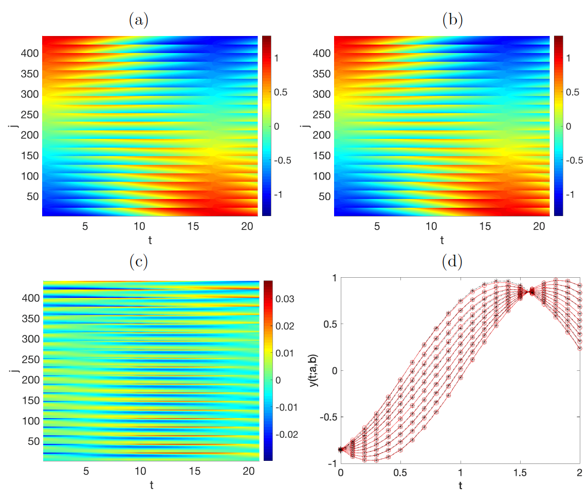
Consider the second order differential equation \[\begin{align} y''(t) + k y(t) = 0, \quad t \in [0,2] \\ y(0) = a, \; y'(0) = b, \end{align}\] for \((a,b) \in [-1,1]\). We wish to approximate the solution \(y(t;a,b)\), which depends continuously on \(a\) and \(b\). We fix \(k=4\) and define a mesh \(t_\ell=(\ell-1) \, \delta t\), \(\delta t =0.1\), \(\ell=1,\ldots,21\). Then, we define the function \[\begin{align} \begin{array}{llll} F: & \mathbb{R}^2 & \rightarrow & \mathbb{R}^{21} \\ & (a,b) & \rightarrow & (y(t_\ell;a,b))_{\ell=1}^{21} \end{array} \end{align}\] and seek a residual neural network approximant. To construct it, we use data for a grid \((a_r,b_s)\) with step \(da=db=0.1\), \(a_r=-1+ (r-1) \, da\), \(b_s=-1+(s-1) \, db\), \(r,s=1, \ldots, 21\), that is, we assume we know the values \(y(t_\ell;a_r,b_s)\) for \(r,s,\ell\). In fact, there are well known explicit expressions for the solutions of this problem \[\begin{align} y(t;a,b) = a cos(2t) + b/2 sin(2t), \quad t>0. \end{align}\] Relabelling \(x_{rs}=(a_r,b_s)\) with a single index \(j=S (r-1) + s\), we get the data \(F(x_j) = y_j\), \(j=1,\ldots,J\), \(J=441\), \(S=21\). We seek a ResNet given by (1 ) with \(N=2\), \(M=21\), using for instance \(L=1\) layer and \(q=5\) units, with sigmoidal activation function \(\sigma\). We characterize \(g: \mathbb{R}^N \rightarrow \mathbb{R}^M\) by a matrix \(\mathbf{G} \in {\cal M}_{MxN}(\mathbb{R})\). The parameters \(\boldsymbol{\gamma}\) to be identified are the coefficients of \(\mathbf{G}\), \(\mathbf{W}^{(1)}\), \(\mathbf{V}^{(1)}\) and \(\mathbf{b}^{(1)}\). We consider the cost (2 ) and solve the gradient system (3 ). For the starting point, we generate a collection or random values and select the proposal with smallest cost. The gradient system converges quite fast to an equilibrium, providing all the coefficients of the neural network. The system was solved with MATLAB routine ode23 and the cost consistently decreased. We stopped the evolution when variations in the cost fell below a tolerance. It took about 5 minutes on a common laptop. Figure 1 illustrates the performance of the calculated approximant on the training mesh and outside it, but remaining in the compact set \([-1,1]^2\).

4.2 Inversion problems constrained by partial differential equations↩︎

Consider a wave equation \[\begin{align} \begin{array}{ll} u_{tt} - c^2 u_{xx} = 0, & x \in \mathbb{R}, t > 0, \\[1ex] u(0,x) = h \exp(-10 w \, (x-1)), & x \in \mathbb{R}, \\[1ex] u_t(0,x) = 0, & x \in \mathbb{R}, \end{array} \label{wave} \end{align}\tag{5}\] with parameters \(h \in [1,2]\), \(w \in [1,2]\), \(c \in [0.1, 2]\). The forward problem consists in finding the solution \(u(x,t)\) of this equation given parameters \((h,w,c)\). It has a well known explicit expression \[\begin{align} u(t,x;h,w,c) = {u(0,x+ct;h,w,c) + u(0,x-ct;h,w,c) \over 2}, \quad x \in \mathbb{R}, t > 0. \end{align}\] The inverse problem consists in finding the parameters \((h,w,c)\) given the solution \(u\). In practice, one considers finite dimensional approximations of \(u\), or just values \(d_{r,\ell}\), \(r=1,\ldots,R\), \(\ell=1,\ldots,{\cal L}\), at a finite collection of points. We wish to approximate a function \(f: \mathbb{R}^{R\times S} \rightarrow \mathbb{R}^3\). Without considering the well posedness of this type of inverse problems, we just see if we can construct a residual neural network approximant.

We introduce a mesh \(t_\ell=(\ell-1) \, \delta t\), \(\delta t =0.1\), \(\ell=1,\ldots,21\), and consider the values at \(x_0=0\), \(x_2=2\). Then, we define the function \[\begin{align} \begin{array}{llll} F: & \mathbb{R}^{42} & \rightarrow & \mathbb{R}^{3} \\ & \mathbf{u}= (u(x_0,t_\ell), u(x_1,t_\ell))_{\ell=1}^{\cal L} & \rightarrow & (h(\mathbf{u}),w(\mathbf{u}),c(\mathbf{u})) \end{array} \end{align}\] and seek a RNN approximant.

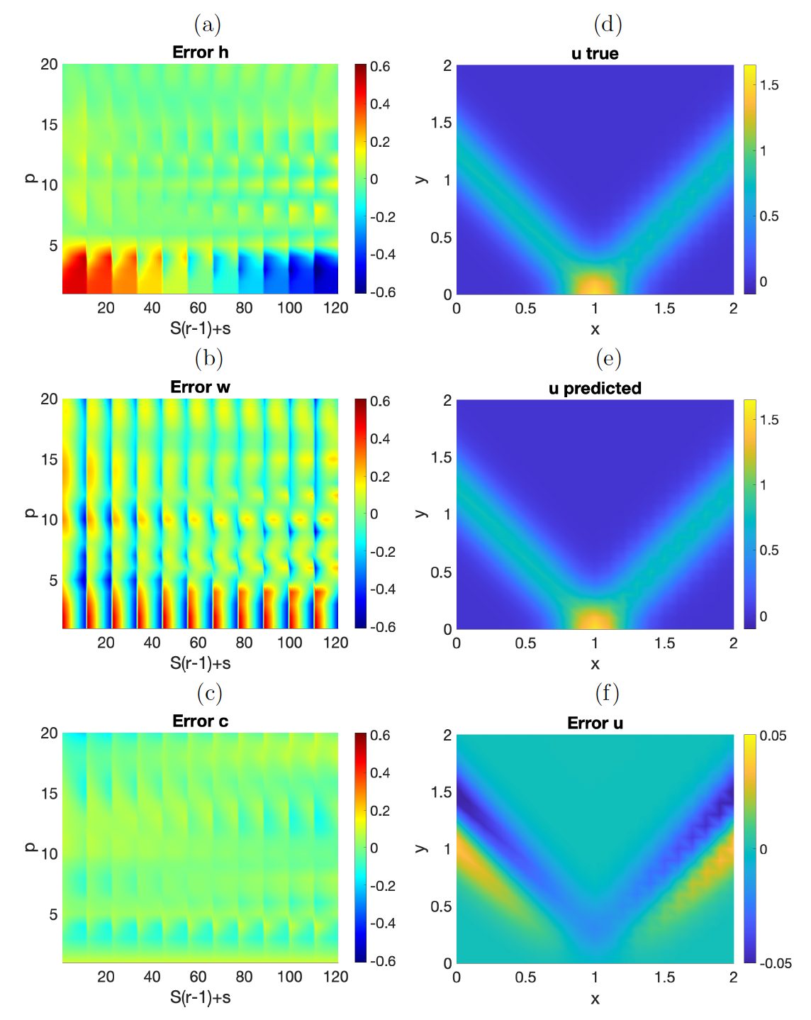
To train the network we generate data on a grid of step \(0.1\) in \([1,2]^2 \times [0.1,2]\). We vary \((h,w,c)\) in the grid and calculate \[\begin{align} \mathbf{u}_{r,s,p}=(u(x_0,t_\ell;h_r,w_s,c_p), u(x_1,t_\ell,h_r,w_s,c_p))_{\ell=1}^{\cal L}, \quad x_0=0, x_1=2. \label{datainv} \end{align}\tag{6}\] Relabelling with a single index \(j=PS(r-1)+ P(s-1)+ p\), we get the data \(F(\mathbf{u}_j)= \mathbf{y}_j\), \(j=1,\ldots,J\), \(J=RSP=2420\), \(R=S=11\), \(P=20\). We seek a ResNet given by (1 ) with \(N=42\), \(M=3\), using for instance \(L=1\) layer and \(q=5\) units, with sigmoidal activation function \(\sigma\). Again, we characterize \(g: \mathbb{R}^N \rightarrow \mathbb{R}^M\) by a matrix \(\mathbf{G} \in {\cal M}_{MxN}(\mathbb{R})\). The parameters \(\boldsymbol{\gamma}\) to be identified are the coefficients of \(\mathbf{G}\), \(\mathbf{W}^{(1)}\), \(\mathbf{V}^{(1)}\) and \(\mathbf{b}^{(1)}\). We solve the gradient system (3 ) for the cost (2 ). To initialize, we generate a collection of random values and select the proposal with smallest cost. The gradient system converges to an equilibrium, providing all the coefficients of the network.

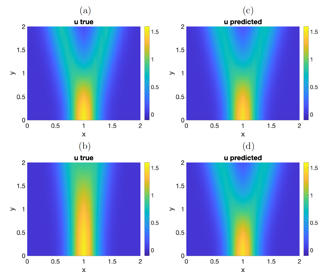
Figure 2 illustrates the performance of the calculated approximant. Predictions worsen for low values of \(c\). Notice that, for low values of \(c\), the wave pattern is different, compare Figure 3 (a)-(b) to Figure 2 (d). The wave does not reach \(x=0\) and \(x=2\) in the given time \(T=2\). If we restrict our RNN fitting to the range of velocities \(c\) for which the wave pattern reaches \(x_0=0\) and \(x_1=2\) for \(t \leq 2\), then the wave predictions are reasonable. However, variations in the signal (6 ) collected at \(x=0,2\) for smaller \(c\) are not expected to suffice to distinguish \(c,h,w\) in the given time interval \([0,T]\). In spite of that, our RNN approximant produces a prediction, as seen in panels (c) and (d) of figure 3. The prediction is noticeably worse for \(c=0.1\) because the pattern has a different shape, but it is still reasonable for \(c=0.2\) even if the signal recorded for that value contain no information.

5 Dataset reduction↩︎

The previous section trains networks using data generated in equispaced parameter meshes. As the parameter range and the number of parameters increase, the amount of data grows fast and training networks becomes more costly. However, the information contained in the data may be redundant. Latin hypercube sampling (LHS) of the parameter space furnishes an strategy to reduce the amount of data while preserving the quality [38].

A square grid is a Latin square if and only if there is only one sample in each column and each row. Latin hypercubes generalize this concept to an arbitrary number of dimensions: each sample is the only sample in each axis-aligned hyperplane containing it. One must decide the number of sample points to use and remember in which row and column each sample point was taken. When sampling functions of \(N\)variables, we divide the range of each variable into \(M\) equally probable intervals. Then, we distribute \(M\) sample points satisfying the Latin hypercube requirements. The number of divisions \(M\) must be equal for each variable. In this way, we do not require more samples for more parameter dimensions.

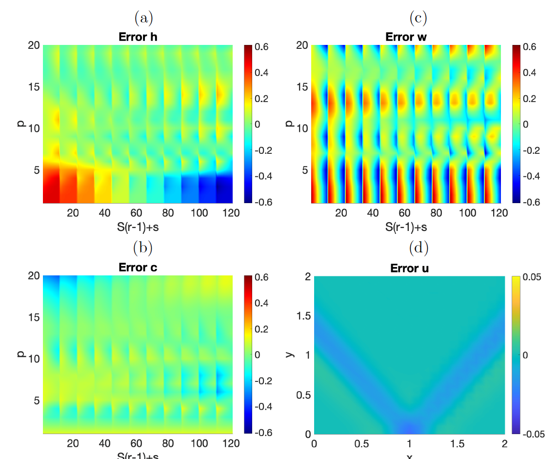
Figure 4 is the counterpart of 2 using \(1210\) data points instead of \(2420\). A similar cost value is reached three times faster. For the particular values of \((h,w,c)\) chosen, the approximation of the solution is even better. However, panels (a)-(c) show that the overall approximation for general values of \((h,w,c)\) can be worse. Notice that the cost functions are different since we consider less points. We can reduce further the cost values and get approximations comparable to those in Figure 3 (a)-(c) in a similar number of steps but in two thirds of the time.

6 Conclusions↩︎

We propose a strategy to train neural networks involving analytic activation functions based on gradient flows. Convergence to a solution is ensured by Lojasiewicz theory. The main advantage is simplicity of implementation. We illustrate the procedure training residual neural networks for simple parametric problems: an ordinary differential equation and an inversion problem defined by a wave equation, both involving a few parameters. Residual neural networks are powerful approximants even for small number of nodes. Simple codes to solve gradient systems of ordinary differential equations allow us to fit the coefficients of the networks yielding reasonable approximants in the tests considered. Latin hypercube sampling can help to reduce the size. Interestingly, the neural network trained for the inverse problem provides predictions of the parameters governing the wave even for ranges where the data contain basically no information to invert, which constitutes a remarkable regularizing effect. In general, the quality of the approximant worsens when different patterns appear as we vary the parametric regime. Otherwise it appears to be quite uniform.

Acknowledgements.↩︎

This research was partially supported by the FEDER/ MICINN-AEI grants PID2020-112796RB-C21 and and PID2024-155528OB-C21.

References↩︎