Intuitionistic Dynamic Logic
July 15, 2026

Faculty of Sciences
Department of Mathematics: Analysis, Logic and Discrete Mathematics
Intuitionistic Dynamic Logic
Lukas Zenger
Supervisor: Prof. Dr. Andreas Weiermann
Co-Supervisor: Prof. Dr. Thomas Studer
Co-Supervisor: Prof. Dr. David Fernández-Duque
Dissertation submitted in fulfilment of the requirements for the degree of
Doctor of Science: Mathematics
Academic year 2025–2026
Preface↩︎
This thesis is the culmination of my doctoral studies in computer science at University of Bern between March 2021 and May 2024 and in mathematics at Ghent University between October 2024 and August 2025. My research was conducted under the supervision of Prof. Dr. Andreas Weiermann, Prof. Dr. Thomas Studer and Prof. Dr. David Fernández-Duque.
This thesis investigates a family of intuitionistic modal logics extended with fixed point operators. Such logics are used to reason about dynamic phenomena, such as the change within a mathematical system over time, the change of state in an automaton after a program step or the change of an agent’s knowledge after an information update. For this reason I refer to them as intuitionistic dynamic logics, where the term ‘dynamic’ highlights their role in formalizing processes of change. At the origin of my doctoral studies stood the goal to develop a coherent mathematical theory of intuitionistic temporal logics, whose modal and fixed point operators capture temporal properties such as ‘in the next time step’ or ‘eventually in the future’. As it often happens in theoretical research, my interests expanded over the course of my PhD, leading me to study related systems such as intuitionistic epistemic logic, bi-intuitionistic modal logic and intuitionistic modal logic with the master modality. All of these logics are discussed in detail in this thesis.
Although logic lies at the intersection of mathematics, philosophy and computer science, the focus here is primarily mathematical. A significant part of the thesis is devoted to the proof theory of intuitionistic dynamic logics, which is studied using Hilbert-style axiomatizations as well as non-wellfounded and cyclic sequent calculi. The latter two are proof systems that allow formal proofs to be infinitely long. Such infinite proofs are particularly well-suited to handle the infinite nature of fixed point operators, but they present considerable technical challenges. The remaining part of the thesis addresses model theoretic and computational aspects of intuitionistic dynamic logics, including expressivity, finite model property, decidability and complexity results.
Intuitionistic modal and dynamic logics are also relevant from a philosophical point of view. While I am interested in the philosophy of intuitionism and questions regarding intuitionistic justifications for modalities, such considerations are not included in the thesis. In fact, the intuitionist shall be warned: I use a classical metatheory when reasoning about intuitionistic dynamic logics and I do not attempt to provide an intuitionistic reading of the studied modalities.
Acknowledgments I would like to express my gratitude to the many people who have contributed to my thesis and my life in general during the past four years. First of all, I would like to thank my supervisors, Andreas Weiermann, Thomas Studer and David Fernández-Duque, for their guidance and help throughout my doctoral studies. Thomas, who was my main supervisor during the three years spent at the University of Bern, has helped me greatly to improve as a logician. I am particularly grateful for his course on proof theory, that he held on my request, which helped me learn about areas of proof theory that I had missed in my previous education. As a supervisor, he always provided me with the help I needed while at the same time giving me the academic freedom to pursue my own interests and learn to work independently. I am also grateful for his wise council regarding the many difficulties that I encountered during my doctoral studies. To Andreas, who was my main supervisor at Ghent University, I am particularly grateful that he provided to me the opportunity to continue my doctoral studies for an additional year after my funding ran out in Bern. This allowed me to bring my PhD to a satisfying conclusion. I would also like to thank him for his efforts organizing my defense and ensuring a smooth transition from Bern to Ghent. To David I would like to express my gratitude for his guidance and help in writing some of the papers that lead to this thesis. His impressive mathematical abilities and great ideas have contributed significantly to many of the results presented in the thesis and his explanations to my understanding of the topic. I also sincerely appreciate his council regarding the writing of this thesis and the suggestion for the title.
I thank the members of the examination committee for reading my thesis and the many helpful comments to improve it: Iris van der Giessen, Bahareh Afshari, Martín Diéguez Lodeiro, Seyedmojtaba Mojtahedi and Giovanni Solda.
I am deeply obliged to my co-authors for their contribution to my thesis: To Jan Rooduijn, Lide Grotenhuis, Brett McLean, David Fernández-Duque, Graham E. Leigh, Borja Sierra Miranda, Bahareh Afshari and Thomas Studer. I am very lucky to have had the opportunity to work with so many talented logicians and hope to continue our collaboration in the future. At this place a special thanks goes to Bahareh, who has guided my academic journey ever since I started my master’s degree in Amsterdam. As my master’s thesis supervisor, she introduced me to the topic of modal fixed point logics, helped me find a PhD position and continued her support throughout my doctoral studies. I also thank the logic groups in Bern and Ghent for the good working atmosphere, the interesting seminars and the social activities.
The last four years have by no means been easy for me. Apart from the pressure and the relative solitude that a PhD life brings, I have also struggled with my mental health. It is important in such situations to have a good social network. Luckily, I
have been blessed with good friends and a supportive family. I would like to thank my parents Christoph and Beatrice for their continued support throughout my entire life and in particular in the recent weeks and months. I thank my brother Michael and his
(soon to be) wife Luza for their care and visits after the submission of my thesis. A special thanks goes to my friends who have always supported me despite my struggles. Thank you Bas, Wijnand, Hugh Mee, Simon, Gabriel, Jiajia, Alessandro, Raphael,
Tianwei, Irina, Massimo, Tong and Freddy.
Lukas Zenger
Bern, October 2025
1 Introduction↩︎
The subject of this thesis is intuitionistic dynamic logic: a family of logical systems characterized by two key features. First, they extend intuitionistic propositional logic with modalities and with fixed point operators. As such they are intuitionistic versions of modal fixed point logics. Second, they provide a formal framework for reasoning about change, whether in mathematical structures evolving over time or in the knowledge state of an agent after an information update. This chapter offers an informal overview of intuitionistic dynamic logics, outlines the motivation for their study, and summarizes the main contributions of the thesis. The formal definitions and results are developed in the subsequent chapters.
1.1 What Are Intuitionistic Dynamic Logics?↩︎
Intuitionistic dynamic logics build on two foundations: intuitionistic logic and intuitionistic modal logic, further enriched with fixed point operators.
Intuitionistic propositional logic (\(\mathsf{IPL}\)) shares the language of classical propositional logic (\(\mathsf{CPL}\)) but deviates from the latter in one crucial aspect: classical logic assumes the law of excluded middle, which states that for any proposition \(p\), the formula \(p \vee \neg p\) is true. As a consequence, every formula in classical logic is considered to be either true or false. Intuitionistic logic, on the other hand, rejects the law of excluded middle, which makes it a proper subsystem of \(\mathsf{CPL}\). Intuitionistic logic was developed by Heyting [1]–[3] with regard to the foundations of mathematics and has emerged as the logical basis of constructive mathematics [4]. \(\mathsf{IPL}\) has also found other interpretations based on topology, computation and, most relevant here, information.
In the information based interpretation of \(\mathsf{IPL}\) due to Kripke [5], an information state is a set \(w\) of propositions, each representing a piece of information available at \(w\). Propositions absent from \(w\) are not considered false but rather unsupported by the available data. The law of excluded middle is therefore not expected to hold, which motivates the use of intuitionistic instead of classical logic to reason about information. Kripke introduced formal semantics for \(\mathsf{IPL}\) based on information orderings: tuples \((W, \leq)\) where \(W\) is a set of information states and \(w \leq v\) means that the information state \(v\) contains all information of \(w\) and possibly more. In this semantics truth is monotone in \(\leq\): if \(w \models \varphi\) and \(w \leq v\), then \(v \models \varphi\). The evaluation of implications is given by \(w \models \varphi \rightarrow \psi\) if for all \(v \geq w\) if \(v \models \varphi\), then \(v \models \psi\). An implication \(\varphi \rightarrow \psi\) thus expresses the consequences of gaining information: \({w \models \varphi \rightarrow \psi}\) expresses that whenever \(w\) is extended by information making \(\varphi\) true, the information also makes \(\psi\) true.
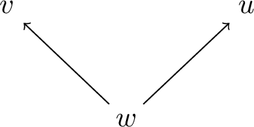
Example 1.1. Let \(w\) be an information state which contains all current mathematical knowledge and consider the P vs. NP problem. Clearly, the statements \(P = NP\) and \(P \not = NP\) are absent in \(w\), since the conjecture is unresolved. Two extensions of \(w\) are therefore \(v\) (containing \(P = NP\)) and \(u\) (containing \(P \not = NP\)). The information ordering is depicted in Figure 1. A well-known result in complexity theory states that if \(P=NP\), then also \(NP = coNP\), implying that \(NP=coNP\) is contained in \(v\) as well. Hence \(w \models (P= NP) \rightarrow (NP = coNP)\). This formula therefore expresses a true statement about the consequences of gaining the information \(P=NP\) at \(w\).
Intuitionistic modal logic (\(\mathsf{IML}\)) extends \(\mathsf{IPL}\) by modal operators, typically \(\larger[-1.5]\square\) and \(\larger[-1.5]\Diamond\). Traditionally, \(\larger[-1.5]\square\varphi\) expresses that \(\varphi\) is necessarily true and \(\larger[-1.5]\Diamond\varphi\) that \(\varphi\) is possibly true. Other interpretations include \(\larger[-1.5]\square\varphi\) as \(\varphi\) is known in epistemic logic or \(\varphi\) is true in the next time step in temporal logic. Semantically, \(\mathsf{IML}\) employs dynamic models which are based on information orderings \((W, \leq)\) extended with a binary relation \(R \subseteq W \times W\). In difference to classical logic, where truth is static, the evaluation of formulas on dynamic models takes into account higher worlds relative to \(\leq\) as well as the worlds accessible over \(R\). Truth in \(\mathsf{IML}\) is therefore dynamic.
The information theoretic interpretation of \(\mathsf{IPL}\) naturally extends to \(\mathsf{IML}\), where the relation \(R\) is used to model non-monotonic information updates (e.g. updates that revise or discard information). The formula \(\larger[-1.5]\Diamond\varphi\) expresses that there exists an update after which \(\varphi\) is true, while \(\larger[-1.5]\square\varphi\) expresses that \(\varphi\) is true after every update. This yields the interpretation of \(\mathsf{IML}\) as logics to reason about monotone and non-monotonic information updates.
The study of intuitionistic modal logic originated in the seminal work of Fitch [6] in 1948. Since then \(\mathsf{IML}\) has grown into an active research area within logic, motivated by philosophical reasons [7]–[9] and by applications to computer science [10]–[12].
Intuitionistic dynamic logics further extend \(\mathsf{IML}\) with the capacity to express infinitary properties. To that end the language is extended by operators whose truth conditions are characterized as fixed points of specific functions, yielding the name fixed point operators. Such operators are not definable in the language of \(\mathsf{IML}\) and significantly increase its expressive power.
Example 1.2. In the information theoretic interpretation of \(\mathsf{IML}\), \(w \models \larger[-1.5]\square\varphi\) expresses that \(\varphi\) is true after any information update of \(w\). Moreover, \(w \models \larger[-1.5]\square^n \varphi\) where \[\larger[-1.5]\square^n \varphi = \underbrace{\larger[-1.5]\square\ldots \larger[-1.5]\square}_{n \text{ times }} \varphi\] expresses that \(\varphi\) is true after any \(n\) updates. The statement that \(\varphi\) is true after any finite number of updates is, however, not expressible, since such a statement corresponds to the infinite formula \[\label{e:32introduction1} \bigwedge_{n < \omega} \larger[-1.5]\square^n \varphi = \varphi \wedge \larger[-1.5]\square\varphi \wedge \larger[-1.5]\square^2 \varphi \wedge \ldots\qquad{(1)}\] which is not well-formed. A fixed point operator \(\ooalign{\larger[-1.5]\square\cr \hidewidth\raise.035ex* \mkern 1.12mu\cr}\) called master modality* compactly expresses this infinite statement by equating \(\ooalign{\larger[-1.5]\square\cr \hidewidth\raise.035ex* \mkern 1.12mu\cr}\varphi\) to the infinite conjunction above.*
Apart from the master modality, many other fixed point operators will be encountered in this thesis, most notably in the context of temporal logics. Here, fixed point operators are used to express statements about the future, such as ‘eventually in the future, something will be the case’ or ‘henceforth in the future, something will always be the case’. Similar to the study of classical modal fixed point logics, most notably the modal \(\mu\)-calculus (see e.g. [13]), the addition of fixed point operators to \(\mathsf{IML}\) does not only increase the expressivity of the resulting logics, but also the difficulty of their mathematical theory, mostly due to the infinite nature of these operators. An overview of the state of the art of the study of intuitionistic dynamic logic is provided in the following subsection.
1.2 State of the Art↩︎
In difference to the study of intuitionistic modal logic, the study of intuitionistic dynamic logic is arguably still in its infancy. However, in recent years several intuitionistic dynamic logics have been introduced and studied in the literature. Among those are intuitionistic versions of temporal logic, which have been mainly studied in two different contexts: metaprogramming and topological dynamics. The former involves the addition of temporal operators to \(\lambda\)-calculi to model aspects of metaprogramming such as staged computation (see e.g. [14]–[16]). The latter is of particular interest to this thesis and dates back to the topological logic project. This project aims to develop computationally well-behaved logical systems to reason about topological dynamic systems, i.e. topological spaces equipped with a continuous function, with potential applications in automated theorem proving in mind. Topological dynamic systems are applied in diverse fields ranging from biology to theoretical computer science. The origin of the project dates back to the seminal work of Artemov, Davoren and Nerode [17] in the late 1990’s, who introduced a classical modal logic and showed how to interpret formulas on topological dynamic systems. In particular, the logic features a standard modal box operator interpreted as the interior operator on topological spaces in the sense of Tarski [18] as well as a modal operator ‘next’ to reason about the continuous function \(f\). Their logic was extended by Kremer and Mints [19] with the fixed point point ‘henceforth’ to reason about the asymptotic behaviour of \(f\), resulting in a logic called dynamic topological logic (\(\mathsf{DTL}\)). Unfortunately, \(\mathsf{DTL}\) was later shown to be undecidable [20], with which interest in \(\mathsf{DTL}\) waned. In 2018, Fernández-Duque introduced an intuitionistic version of linear temporal logic, called \(\mathsf{iLTL}\) in this thesis, and showed that it enjoys a natural interpretation both over topological dynamic systems as well as dynamic models based on information orderings [21]. Furthermore, he established the decidability of \(\mathsf{iLTL}\), thus providing a decidable logic capable of expressing interesting properties of topological dynamic systems. The logic \(\mathsf{iLTL}\) is an extension of intuitionistic propositional logic with a modality ‘next’ as well as a fixed point operator ‘eventually’ and thus an intuitionistic dynamic logic in our sense. It was later shown that \(\mathsf{iLTL}\) admits a sound and complete axiomatization [22] and that \(\mathsf{iLTL}\) extended with additional fixed point operators remains decidable [23]. The proof theory of \(\mathsf{iLTL}\), however, remains largely unexplored, with the exception of a cyclic sequent calculus introduced recently by Menéndez Turata in his PhD thesis [24].
Apart from intuitionistic temporal logics, intuitionistic dynamic logics have also been studied in an epistemic setting. Jäger and Marti introduced an intuitionistic version of common knowledge logic called \(\mathsf{ICK}\) [25], [26], which extends intuitionistic propositional logic by modal operators \(\mathsf{K}_i\), where \(\mathsf{K}_i \varphi\) expresses that an agent \(i\) knows \(\varphi\), as well as a fixed point operator expressing a powerful notion of group knowledge called common knowledge. Furthermore, variants of \(\mathsf{ICK}\) with operators for distributed knowledge were also studied in [27]–[29]. In difference to \(\mathsf{iLTL}\), the work in \(\mathsf{ICK}\) is primarily proof theoretic, highlighted by the development and study of axiomatizations and sequent calculi. Artemov and Protopopescu introduced a different version of intuitionistic epistemic logic called \(\mathsf{IEL}\) [8]. In difference to \(\mathsf{ICK}\), which treats knowledge as in the classical case, Artemov and Protopopescu aim to give an intuitionistic reading to knowledge, resulting in a substantially different logical systems.
Last but not least, intuitionistic versions of the modal \(\mu\)-calculus have recently been studied by Pacheco [30] who focuses on game semantics and by Afshari and Grotenhuis [31] who develop non-wellfounded and cyclic proof systems for intuitionistic \(\mu\)-calculus with the Lewis arrow.
1.3 Motivation↩︎
The original motivation for the research presented in this thesis is related to the dynamic topological logic project and the logic \(\mathsf{iLTL}\). As mentioned in the previous subsection, the proof theory of \(\mathsf{iLTL}\) is largely unexplored, a gap which needs to be filled when it comes to application in automated theorem proving. Moreover, while a sound and complete axiomatization for \(\mathsf{iLTL}\) was provided in [22], the problem of finding an axiomatization for the extended language with ‘henceforth’ has remained open for several years. Importantly, while the set of validities of \(\mathsf{iLTL}\) evaluated over topological models coincides with the set of validities over dynamic models based on information orderings, the same is not true in the extended language (see Chapter 6). The main goal of this thesis was therefore to develop the proof theory of \(\mathsf{iLTL}\) and a sound and complete axiomatization for the extended language of \(\mathsf{iLTL}\) with ‘henceforth’, in the setting of dynamic models based on information orderings. The presence of fixed point operators complicates this venture, due to the fact that proof systems require a formal counterpart to induction to reason about fixed point operators. Luckily, modal fixed point logics have been studied extensively in the classical realm and it is the methods developed there that come to the rescue. In the classical realm, automata, games, non-wellfounded and cyclic proofs as well as semantic techniques such as filtrations and simulations have proven suitable for the study of fixed points in modal logic [32]–[34]. Little is known, however, whether these techniques are applicable to the intuitionistic case. In fact, it can be expected that the application of such methods is significantly complicated, due to the underlying intuitionistic logic and the more complicated mathematical structures used to evaluate formulas (i.e. dynamic models). A second motivation, based in mathematical curiosity, is therefore to investigate how to adapt such techniques, in particular non-wellfounded and cyclic proofs, to the intuitionistic case, with the hope that our findings will not only provide a rigorous mathematical theory for \(\mathsf{iLTL}\), but also prove useful for the study of other, related logical systems. Thus the second motivation naturally leads to a third one, which is to explore related logics and to adapt the techniques developed for \(\mathsf{iLTL}\) to these systems.
From a more general perspective, intuitionistic modal and dynamic logics have found tangible applications in computer science, for example to model aspects of metaprogramming such as staged computation [12], [14], [15], [35]–[37] and to philosophy, for example to give an intuitionistic account of knowledge [8], [9], [38]. Furthermore, the information theoretic interpretation of intuitionistic dynamic logics opens the possibility for applications to artificial intelligence, such as to knowledge representation, (epistemic) planning or logic programming. These applications in turn motivate the development of a rigorous mathematical theory, and in particular well-behaved proof systems that facilitate proof-search algorithms. Moreover, applications to computer science lead to the study of the computational properties of intuitionistic dynamic logics.
1.4 Contributions↩︎
This thesis studies five intuitionistic dynamic logics:
Intuitionistic master modality (\(\mathsf{IM}\)): an intuitionistic dynamic logic which extends \(\mathsf{IPL}\) by a single modality \(\larger[-1.5]\square\) and the aforementioned master modality \(\ooalign{\larger[-1.5]\square\cr \hidewidth\raise.035ex* \mkern 1.12mu\cr}\).
Intuitionistic common knowledge logic (\(\mathsf{ICK}\)): an intuitionistic version of epistemic logic with common knowledge introduced by Jäger and Marti [25].
Intuitionistic linear temporal logic (\(\mathsf{iLTL}\)): an intuitionistic version of linear temporal logic introduced by Fernández-Duque [21].
Bi-intuitionistic modal logic (\(\mathsf{biML}\)): an extension of \(\mathsf{IPL}\) with modalities \(\larger[-1.5]\square\) and \(\larger[-1.5]\Diamond\) as well as the co-implication connective from bi-intuitionistic logic.
Bi-intuitionistic linear temporal logic (\(\mathsf{biLTL}\)): a bi-intuitionistic version of linear temporal logic.
Apart from introducing new logics, namely \(\mathsf{biML}\) and \(\mathsf{biLTL}\), the main contributions of this thesis are threefold: semantic, syntactic and computational.
On the semantic side we study various classes of dynamic models which satisfy different confluence conditions and frame conditions. The former are interaction principles between \(\leq\) and \(R\), which play an important role in the study of intuitionistic modal logics. The latter are conditions placed on \(R\), such as transitivity. We establish expressivity results, and show that several logics satisfy the finite model property. The most important contribution is the proof of the finite model property for \(\mathsf{biML}\) and \(\mathsf{biLTL}\), which is shown via an intricate combinatorial analysis of the semantics by employing labelled and quasi models.
On the syntactic side, we develop several proof systems in form of Hilbert-style axiomatizations as well as cyclic and non-wellfounded sequent calculi. We show how to adapt classical techniques such as canonical model constructions and proof search arguments to obtain soundness and completeness results. In some cases, such as for \(\mathsf{IM}\) or for \(\mathsf{ICK}\), an adaption is relatively straightforward. For other cases, however, such as \(\mathsf{biLTL}\), adapting the classical techniques to obtain completeness is not possible and we are forced to develop different methods. We highlight the development of a sound and complete axiomatization for an extension of the language of \(\mathsf{iLTL}\) with the fixed point operator ‘henceforth’; a problem that has been open for several years.
Finally, on the computational side, we establish decidability and complexity results for the problem of checking validity for several intuitionistic dynamic logics. The most important results are, on the one hand, a precise complexity bound for \(\mathsf{ICK}\) over S5 models, and on the other hand, the proofs that \(\mathsf{biML}\) and \(\mathsf{biLTL}\) are decidable.
1.5 Structure of the Thesis and Sources of the Material↩︎
Chapter 2 serves as an introduction to the mathematical formalisms that are used throughout the thesis. In particular we formally introduce \(\mathsf{IPL}\) and \(\mathsf{IML}\), provide a brief introduction to proof theory and discuss fixed point operators. Furthermore the history of \(\mathsf{IPL}\) and \(\mathsf{IML}\) is discussed. Chapters 3 - 6 each study one of the five intuitionistic dynamic logics mentioned before. Chapters 3 - 5 are based on [39]–[41]; the first two are joint publications with Bahareh Afshari, Lide Grotenhuis and Graham E. Leigh and the last is a joint publication with Jan Rooduijn. Chapters [c: bi-int ml new] and 6 are based on [42], [43], both of which are joint publications with David Fernández-Duque and Brett McLean. A joint publication with Borja Sierra-Miranda and Thomas Studer [44] about non-wellfounded proof theory is not discussed in this thesis.
2 Preliminaries↩︎
This chapter introduces the logical systems upon which the thesis is built. We begin by setting up notational conventions and basic definitions. Then we formally introduce intuitionistic propositional logic, in particular its syntax and its semantics, which is defined over intuitionistic Kripke models. Moreover, we give a general definition of proof system and introduce a Hilbert-style axiomatization and a Gentzen-style sequent calculus for intuitionistic propositional logic; the axiomatizations and sequent calculi presented later on are based on these two systems. Afterwards we formally introduce intuitionistic modal logic, namely its syntax and its semantics, which is defined over dynamic models: extensions of intuitionistic Kripke models by a modal accessibility relation. Furthermore, we discuss a range of confluence conditions and frame conditions. Finally, we discuss fixed point operators and then finish the chapter with a historical overview of intuitionistic (modal) logic.
2.1 Basic Definitions↩︎
This section introduces the notation and the basic mathematical objects, such as partial functions or trees, used throughout the rest of the thesis.
We denote the set of natural numbers by \(\omega\) and write \(n < \omega\) to denote that \(n\) is a natural number. Given a set \(X\), the power set of \(X\) is denoted by \(\mathcal{P}(X)\) and the cardinality by \(\left|X\right|\).
2.1.1 Binary Relations↩︎
Given sets \(X\) and \(Y\) a binary relation is a subset \(R \subseteq X \times Y\) of the cartesian product of \(X\) and \(Y\). Given \(x \in X\) and \(y \in Y\) we write both \((x,y) \in R\) and \(x \mathrel{R}y\) to denote that \(x\) and \(y\) are related by \(R\). Moreover we denote by \(dom(R)\) the domain and by \(ran(R)\) the range of \(R\). Formally, \[\begin{align} dom(R) &\mathrel{\vcenter{:}}= \{ x \in X \mid \text{ there exists } y \in Y \text{ with } x \mathrel{R} y \};\\ ran(R) & \mathrel{\vcenter{:}}= \{ y \in Y \mid \text{ there exists } x \in X \text{ with } x \mathrel{R} y \}.\\ \end{align}\] If \(x \in dom(R)\) we write \(\exists{R(x)}\) and otherwise \(\nexists{R(x)}\). Given \(U \subseteq X\) and \(V \subseteq Y\), we write \[R{\upharpoonright}_{U \times V} \mathrel{\vcenter{:}}= \{(x,y) \in U \times V \mid (x,y) \in R\}\] for the restriction of \(R\) to \(U\) and \(V\). Given two binary relations \(R_1 \subseteq X \times Y\) and \(R_2 \subseteq Y \times Z\), the composition of \(R_1\) with \(R_2\) is denoted by \(R_2 \circ R_1\), formally \[R_2 \circ R_1 \mathrel{\vcenter{:}}= \{(x,z) \in X \times Z \mid \text{ there exists } y \in Y \text{ with } (x,y) \in R_1 \text{ and } (y,z) \in R_2\}.\]
We are interested in specific binary relations, which are introduced below.
Definition 2.1. Let \(X\) and \(Y\) be sets.
A partial function* from \(X\) to \(Y\) is a binary relation \(f \subseteq X \times Y\) which is functional: for all \(x \in X\) and \(y,y' \in Y\) if \((x,y) \in f\) and \((x,y') \in f\), then \(y = y'\).*
A function* is a partial function \(f\subseteq X \times Y\) such that \(dom(f) = X\).*
We denote (partial) functions by \(f: X \longrightarrow Y\) and write \(f(x) = y\) instead of \(x \mathrel{f} y\). Functions are always assumed to be total; whenever a function is partial, we will explicitly say so.
Definition 2.2. Let \(X\) be a set and \(R \subseteq X \times X\).
\(R\) is a partial order* on \(X\) if*
\(R\) is reflexive: for all \(x \in X\): \(x \mathrel{R}x\);
\(R\) is transitive: for all \(x,y,z \in X\): \(x \mathrel{R}y\) and \(y \mathrel{R}z\) imply \(x \mathrel{R}z\);
\(R\) is antisymmetric: for all \(x,y \in X\): \(x \mathrel{R}y\) and \(y \mathrel{R}x\) imply \(x=y\).
\(R\) is a well-order* on \(X\) if*
\(R\) is a partial order on \(X\);
\(R\) is total: for all \(x,y \in X\): \(x \mathrel{R}y\) or \(y \mathrel{R}x\);
Every non-empty \(U \subseteq X\) has a \(R\)-least element: there exists \(x \in U\) such that for all \(y \in U\): \(x \mathrel{R}y\).
\(R\) is an equivalence relation* on \(X\) if*
\(R\) is reflexive;
\(R\) is transitive;
\(R\) is symmetric: for all \(x,y \in X\): \(x \mathrel{R}y\) implies \(y \mathrel{R}x\).
Partial orders and well-orders are denoted by \(\leq\).1 As usual, we write \(x < y\) if \(x \leq y\) and \(x \not = y\). Given a partial order \(\leq\) on \(X\), the tuple \((X, \leq)\) is called a poset. If \(\leq\) is a well-order on \(X\), then \((X, \leq)\) is called a well-ordered set. Given a poset \((X, \leq)\) and \(x \in X\), let \[\begin{align} x^\uparrow &\mathrel{\vcenter{:}}= \{ y \in X \mid x \leq y\}\\ x^\downarrow &\mathrel{\vcenter{:}}= \{ y \in X \mid y \leq x\}. \end{align}\] We call \(x^\uparrow\) the upset of \(x\) and \(x^\downarrow\) the downset of \(x\).
Equivalence relations are denoted by \(\sim\). If \(\sim\) is an equivalence relation on \(X\) and \(x \in X\), the equivalence class of \(x\) is given by \[[x] \mathrel{\vcenter{:}}= \{ y \in X \mid x \sim y\}.\]
The quotient of \(X\) under \(\sim\) is given by \[\frac{X}{\sim} \mathrel{\vcenter{:}}= \{[x] \mid x \in X\}.\]
2.1.2 Trees↩︎
Trees will be used primarily for studying formal proofs. We will usually be quite informal about the precise structure of a tree. Here, the definition of trees and related concepts are introduced.
Definition 2.3. A tree* is a tuple \(\mathcal{T}=(T, \leq, r)\) where*
\((T, \leq)\) is a poset;
\(r \in T\) and for all \(t \in T\): \(r \leq t\);
for all \(t \in T\), \((t^\downarrow, \leq\upharpoonright_{t^\downarrow \times t^\downarrow})\) is a well-ordered set.
Elements of \(T\) are called nodes and \(r\) is called the root. If \(s,t \in T\) with \(s < t\) and there does not exist an \(s' \in T\) with \(s < s' < t\), then \(s\) is called the parent of \(t\) and \(t\) is called a child of \(s\). If \(s < t\), then \(s\) is called an ancestor of \(t\) and \(t\) is called a descendant of \(s\). Nodes without children are called leafs. A path is a sequence of nodes \((t_i)_i\) such that for all \(i\) the node \(t_{i+1}\) is a child of \(t_i\). Given a finite path \((t_i)_{i \leq n}\) for \(n < \omega\), the length \(l((t_i)_{i \leq n})\) of \((t_i)_{i \leq n}\) is defined to be \(l((t_i)_{i \leq n}) \mathrel{\vcenter{:}}= n\). A branch is a path starting at the root which is either infinite or ends in a leaf. A tree \(\mathcal{T}=(T, \leq, r)\) is finite if \(T\) is finite and infinite otherwise. Given a finite tree \(\mathcal{T}\), the height \(h(\mathcal{T})\) of \(\mathcal{T}\) is defined to be \(h(\mathcal{T}) \mathrel{\vcenter{:}}= max\{l(\rho) \mid \rho \text{ is a branch of } \mathcal{T}\}\). A tree \(\mathcal{T}\) is finitely branching if every node of \(\mathcal{T}\) has only finitely many children. The following is a well-known result about finitely branching trees.
Theorem 2.1 (Kőnig’s Lemma). Let \(\mathcal{T}\) be a finitely branching tree. If \(\mathcal{T}\) is infinite, then \(\mathcal{T}\) contains an infinite branch.
A labelled tree is a tree together with a labelling function which assigns to each node a label.
Definition 2.4. Let \(\mathcal{S}\) be a set. A \(\mathcal{S}\)-labelled tree* is a tuple \(\pi = (T, \leq, r, \ell)\) where*
\((T, \leq, r)\) is a tree;
\(\ell: T \longrightarrow \mathcal{S}\) is a function.
The height of a finite labelled tree \((T, \leq, r, \ell)\) is the height of \((T, \leq, r)\). Finally, the following notion of subtree will be used repeatedly.
Definition 2.5. Let \(\mathcal{T}=(T, \leq, r)\) be a tree and \(u \in T\) a node. The subtree of \(\mathcal{T}\) rooted at \(u\)* is the tree \(\mathcal{T}_u = (u^\uparrow, \leq\upharpoonright_{u^\uparrow \times u^\uparrow}, u)\).*
2.2 Intuitionistic Logic↩︎
Every intuitionistic dynamic logic studied in this thesis is an extension of intuitionistic propositional logic with modalities and fixed point operators. We only study propositional logics, therefore we usually call intuitionistic propositional logic simply intuitionistic logic. This section introduces the syntax and semantics of intuitionistic logic (\(\mathsf{IPL}\)). An overview of the history of intuitionistic logic and its many interpretations is deferred to Section 2.6.
The language \(\mathcal{L}_\mathsf{IPL}\) of \(\mathsf{IPL}\) consists of a countable set of atomic propositions \(\mathsf{Prop}\), the constant falsum \(\bot\), the connectives conjunction \(\wedge\), disjunction \(\vee\) and implication \(\rightarrow\) as well as brackets \((\) and \()\). Formulas of \(\mathcal{L}_\mathsf{IPL}\) are given by the following grammar in Backus–Naur form: \[\varphi ::= \bot \, \lvert \, p \, \lvert \, (\varphi \wedge \varphi) \, \lvert \, (\varphi \vee \varphi) \, \lvert \, (\varphi \rightarrow \varphi)\] where \(p \in \mathsf{Prop}\). Formulas (in every system studied subsequently) are always denoted by Greek letters \(\varphi, \psi, \chi\) and \(\gamma\), while propositions are denoted by Latin letters \(p,q,r\). Subscripts are also used such as \(\varphi_1, \varphi_2\) and so on. We write \(\varphi \in \mathcal{L}_\mathsf{IPL}\) to denote that \(\varphi\) is a formula of \(\mathcal{L}_\mathsf{IPL}\). We omit outermost brackets when displaying formulas and simply write e.g. \(\varphi \wedge \psi\) instead of \((\varphi \wedge \psi)\). In fact, brackets will only be used to give unique precedence of the connectives in longer formulas. The connectives negation \(\neg\) and if and only if \(\leftrightarrow\), as well as the constant verum \(\top\) are treated as defined connectives, where \(\top \mathrel{\vcenter{:}}= \bot \rightarrow \bot\), \(\neg \varphi \mathrel{\vcenter{:}}= \varphi \rightarrow \bot\) and \(\varphi \leftrightarrow \psi \mathrel{\vcenter{:}}= (\varphi \rightarrow \psi) \wedge (\psi \rightarrow \varphi)\).
Formulas of \(\mathsf{IPL}\) are evaluated on intuitionistic Kripke models.
Definition 2.6. An intuitionistic Kripke model* is a tuple \(\mathcal{M}=(W, \leq, V)\) where*
\(W\) is a non-empty set;
\(\leq\) is a partial order on \(W\);
\(V: W \longrightarrow \mathcal{P}(\mathsf{Prop})\) is monotone in \(\leq\), i.e. for all \(w, v \in W\): \[w \leq v \text{ implies } V(w) \subseteq V(v).\]
Intuitionistic Kripke models are usually simply called Kripke models and denoted by \(\mathcal{M}\) and \(\mathcal{N}\). Elements of \(W\) are called worlds or (information) states and are denoted by \(w,v,u\) and so on. The relation \(\leq\) is called the intuitionistic order and if \(w \leq v\), then we call \(v\) an intuitionistic successor of \(w\). The function \(V\) is called a valuation. A tuple \((\mathcal{M}, w)\) where \(\mathcal{M}=(W, \leq, V)\) is a Kripke model and \(w \in W\) is called a pointed Kripke model.
Remark 2.2. Intuitionistic Kripke models are the mathematical structures based on information orderings mentioned in Chapter 1. The set \(W\) is considered to be a set of information states, where for each state \(w \in W\) the valuation \(V\) assigns to \(w\) the information it contains. The intuitionistic order \(\leq\) models extensions of the information state, where the monotonicity of \(V\) in \(\leq\) guarantees that extensions of \(w\) contain at least as much information as \(w\) itself.
Definition 2.7. The truth relation* \(\models\) between worlds of a Kripke model \(\mathcal{M}= (W, \leq, V)\) and formulas is defined inductively as follows, where \(p \in \mathsf{Prop}\) and \(w \in W\).*
| \(\mathcal{M},w \not \models \bot\) | ||
| \(\mathcal{M},w \models p\) | iff | \(p \in V(w)\) |
| \(\mathcal{M},w \models \varphi \wedge \psi\) | iff | \(\mathcal{M}, w \models \varphi\) and \(\mathcal{M},w \models \psi\) |
| \(\mathcal{M},w \models \varphi \vee \psi\) | iff | \(\mathcal{M}, w \models \varphi\) or \(\mathcal{M},w \models \psi\) |
| \(\mathcal{M},w \models \varphi \rightarrow \psi\) | iff | for all \(v \geq w\) if \(\mathcal{M},v \models \varphi\), then \(\mathcal{M},v \models \psi\) |
If \(\mathcal{M}, w \models \varphi\), then \(\varphi\) is called true* at \(w\).*
A formula \(\varphi\) is called satisfiable over the class of Kripke models if there exists a Kripke model \(\mathcal{M}=(W, \leq, V)\) and a world \(w \in W\) with \(\mathcal{M},w \models \varphi\) and unsatisfiable otherwise. Furthermore, \(\varphi\) is called valid over the class of Kripke models if \(\mathcal{M}, w \models \varphi\) for all Kripke models \(\mathcal{M}=(W, \leq, R)\) and all worlds \(w \in W\) and falsifiable otherwise.
Definition 2.8. The set of valid \(\mathcal{L}_\mathsf{IPL}\)-formulas over the class of intuitionistic Kripke models is denoted by \(\mathbf{IPL}\).
For the defined connectives a simple computation shows that the following truth conditions hold. The proof is omitted.
Lemma 2.1. Let \((\mathcal{M},w)\) be a pointed Kripke model and \(\varphi, \psi \in \mathcal{L}_\mathsf{IPL}\). The following hold.
| \(\mathcal{M}, w \models \top\) | ||
| \(\mathcal{M}, w \models \neg \varphi\) | iff | for all \(v \geq w\), \(\mathcal{M}, v \not \models \varphi\) |
| \(\mathcal{M}, w \models \varphi \leftrightarrow \psi\) | iff | for all \(v \geq w\), \(\mathcal{M}, v \models \varphi\) if and only if \(\mathcal{M}, v \models \psi\) |
A defining property of Kripke semantics for intuitionistic logic is the Monotonicity Lemma, which states that the truth relation is monotone in \(\leq\).
Lemma 2.2 (Monotonicity). Let \(\mathcal{M}=(W, \leq, V)\) be a Kripke model, \(w,v \in W\) worlds and \(\varphi\) a formula. If \(w \leq v\) and \(\mathcal{M}, w \models \varphi\), then \(\mathcal{M}, v \models \varphi\).
Proof. The proof is by induction on the structure of \(\varphi\). The case for \(\varphi= \bot\) trivially holds. For \(\varphi = p \in \mathsf{Prop}\) if \(\mathcal{M}, w \models p\), then \(p \in V(w)\). Since \(w \leq v\), the monotonicity of \(V\) implies that \(p \in V(v)\). Hence \(\mathcal{M}, v \models p\). The cases for \(\varphi = \psi \wedge \chi\) and \(\varphi = \psi \vee \chi\) follow directly from the truth conditions for \(\wedge\) and \(\vee\) and from the induction hypothesis. Suppose \(\varphi = \psi \rightarrow \chi\) and \(\mathcal{M},w \models \psi \rightarrow \chi\). By definition, for all \(u \geq w\) if \(\mathcal{M},u \models \psi\), then \(\mathcal{M},u \models \chi\). If \(u \geq v\), then the transitivity of \(\leq\) implies that \(u \geq w\) and so if \(\mathcal{M}, u \models \psi\), then \(\mathcal{M}, u \models \chi\). Hence \(\mathcal{M}, v \models \psi \rightarrow \chi\). ◻
We finish the section by stating two properties of the Kripke semantics for intuitionistic logic. Recall that the law of excluded middle states that for any proposition \(p\) the formula \(p \vee \neg p\) is valid.
Lemma 2.3. The law of excluded middle does not hold for intuitionistic logic: \(p \vee \neg p\) is not valid over the class of intuitionistic Kripke models.
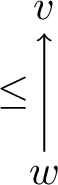
Proof. Consider the intuitionistic Kripke model \(\mathcal{M}=(W, \leq, R)\) where \(W =\{ w, v\}\), \(\leq = \{(w,w), (w,v), (v,v)\}\) and \(V(w) = \emptyset\) and \(V(v) = \{p\}\) (see Figure 2).2 It is clear that \(\mathcal{M}\) is a Kripke model. By definition \(\mathcal{M}, w \not \models p\). Moreover, \(\mathcal{M}, v \models p\), implying that \(\mathcal{M}, w \not \models \neg p\). Hence \(\mathcal{M}, w \not \models p \vee \neg p\). ◻
A Kripke model \(\mathcal{M}=(W, \leq, V)\) is finite if \(W\) is a finite set. Intuitionistic logic satisfies the finite model property if every falsifiable formula can be falsified in a finite Kripke model. The following is for example proven in [45].
Lemma 2.4. Intuitionistic logic satisfies the finite model property.
2.3 Proof systems↩︎
An important tool used in our study of intuitionistic dynamic logics are proof systems. Intuitively, a proof system consists of a set of axioms - formulas assumed to be true without proof - and a set of inference rules - rules that govern how to prove new formulas from axioms and formulas which have already been proven. The rules of a proof system do not refer to the semantics of the logic. Instead they are purely mechanical and dictate how to manipulate the syntactic structure of formulas to obtain new ones. Accordingly, just as the formal semantics of a logic determine the set of valid formulas, a proof system determines the set of provable formulas. The bridge between the semantic and syntactic realm are soundness and completeness proofs: soundness establishes that every provable formula is valid while completeness establishes that every valid formula is provable.
We will study two types of proof systems: (Hilbert-style) axiomatizations and (Gentzen-style) sequent calculi. Regarding the sequent calculi, we will in particular study non-wellfounded and cyclic proofs. This section introduces the basic definitions shared by all systems encountered in the thesis. Afterwards we introduce an axiomatization and a sequent calculus for \(\mathsf{IPL}\). A discussion of non-wellfounded and cyclic proofs is deferred to Chapter 3.
2.3.1 General Definitions↩︎
Some proof systems manipulate formulas while others manipulate more complicated mathematical structures. Therefore we give a general definition of inference rules and proof systems relative to an arbitrary set \(\mathcal{S}\).
Definition 2.9. Let \(\mathcal{S}\) be a set.
A rule instance* (w.r.t. \(\mathcal{S}\)) is a finite tuple \(\langle s, \langle s_1, \ldots, s_n\rangle \rangle\) where \(s, s_1, \ldots s_n \in \mathcal{S}\) and \(0 \leq n < \omega\). The first element \(s\) is called the conclusion and the elements \(s_i\) for \(1 \leq i \leq n\) in the second component are called premises.*
An (inference) rule* \(\mathsf{r}\) (w.r.t. \(\mathcal{S}\)) is a set of rule instances.*
A proof system* \(\mathrm{P}\) (w.r.t. \(\mathcal{S}\)) is a finite set of inference rules.*
Given a rule instance \(\langle s, \langle s_1, \ldots, s_n\rangle \rangle\), its arity is \(n\). Rule instances with arity \(0\) are called axioms. A rule instance \(\langle s, \langle s_1, \ldots, s_n \rangle \rangle \in \mathsf{r}\) is depicted as \[\infer[\mathsf{r}]{s}{s_1 & \ldots & s_n}\] with the intended reading that if the premises \(s_1, \ldots, s_n\) are obtained, then we can derive the conclusion \(s\). Inference rules where each rule instance is an axiom are called axiom schemes. Inference rules that are not axiom schemes are called proper. We will mostly consider inference rules where each rule instance has the same arity.3 Such inference rules will be depicted schematically, i.e. we depict the rule by providing one rule instance from which all other instances can be obtained via uniform substitution.
Definition 2.10. Let \(\mathrm{P}\) be a proof system (w.r.t. \(\mathcal{S}\)) and \(\pi =(T, \leq, r, \ell)\) a \(\mathcal{S}\)-labelled tree. Then \(\pi\) is labelled according to the rules of* \(\mathrm{P}\) if whenever \(t,t_1, \ldots, t_n \in T\) with \(t\) being the parent and \(t_1, \ldots, t_n\) the children of \(t\) in \(\pi\), \(\langle \ell(t), \langle \ell(t_1), \ldots, \ell(t_n)\rangle \rangle\) is a rule instance of a rule in \(\mathrm{P}\).*
The two types of proof systems studied in this thesis are axiomatizations and sequent calculi. These two types of systems differ with respect to the set of elements they manipulate. Axiomatizations manipulate formulas of a logical language (e.g. \(\mathcal{L}_\mathsf{IPL}\)). Sequent calculi, on the other hand, manipulate so called sequents, which have more structure.
2.3.2 An Axiomatization for Intuitionistic Logic↩︎
This subsection introduces an axiomatization for intuitionistic logic. The axiomatization manipulates \(\mathcal{L}_\mathsf{IPL}\)-formulas. An axiomatization typically consist of a list of axiom schemes together with a few proper inference rules. The presented system is taken from [46].
Definition 2.11. The Hilbert-style axiomatization \(\mathrm{IPL_H}\) consists of the inference rules depicted in Table 1.
| \(\mathsf{1:}\) | \(\varphi \rightarrow (\psi \rightarrow \varphi)\) |
| \(\mathsf{2:}\) | \((\varphi \rightarrow (\psi \rightarrow \chi)) \rightarrow ((\varphi \rightarrow \psi) \rightarrow (\varphi \rightarrow \chi))\) |
| \(\mathsf{3:}\) | \((\varphi \wedge \psi) \rightarrow \varphi\) |
| \(\mathsf{4:}\) | \((\varphi \wedge \psi) \rightarrow \psi\) |
| \(\mathsf{5:}\) | \(\varphi \rightarrow (\varphi \vee \psi)\) |
| \(\mathsf{6:}\) | \(\psi \rightarrow (\varphi \vee \psi)\) |
| \(\mathsf{7:}\) | \((\varphi \rightarrow \chi) \rightarrow ((\psi \rightarrow \chi) \rightarrow ((\varphi \vee \psi) \rightarrow \chi))\) |
| \(\mathsf{8:}\) | \(\bot \rightarrow \varphi\) |
| \(\mathsf{MP:}\) | \(\infer{\psi}{\varphi & \varphi \rightarrow \psi}\) |
The rules \(\mathsf{1}\) – \(\mathsf{8}\) are axiom schemes. Instead of writing for example \[\infer[\mathsf{1}]{\varphi \rightarrow (\psi \rightarrow \varphi)}{}\] for an axiom, we prefer to simply write \(\varphi \rightarrow (\psi \rightarrow \varphi)\) when we list the axiomatization to clearly distinguish axiom schemes from proper inference rules. The rule \(\mathsf{MP}\) is the modus ponens rule, which will be featured in all axiomatizations considered in this thesis. It states that from \(\varphi\) and \(\varphi \rightarrow \psi\) we can derive \(\psi\). We implicitly assume that every inference rule is closed under uniform substitution. We will therefore not explicitly add a substitution rule to our systems. In other words, each axiom scheme and inference rule can be instantiated by uniformly substituting the formulas displayed in Table 1 by other formulas. Formal proofs in an axiomatization are called derivations.
Definition 2.12. A derivation* in \(\mathrm{IPL_H}\) of a formula \(\varphi\) is a finite tree \(\pi\) labelled by formulas according to the rules of \(\mathrm{IPL_H}\) such that the root of \(\pi\) is labelled by \(\varphi\) and every leaf of \(\pi\) is labelled by an axiom.*
If there exists a derivation of \(\varphi\), then we write \(\vdash_\mathrm{IPL_H} \varphi\) and say that \(\varphi\) is \(\mathrm{IPL_H}\)-derivable. If the proof system is clear from context, we omit the mention of \(\mathrm{IPL_H}\).
Example 2.1. The formula \(\varphi \rightarrow \varphi\) is derivable in \(\mathrm{IPL_H}\). First, recall that \(\top = \bot \rightarrow \bot\) which is derivable, since it is an instance of \(\mathsf{8}\). Therefore we obtain the following derivation:
It is easy to see that the above structure is a tree labelled by formulas according to the rules of \(\mathrm{IPL_H}\), where the root is labelled by \(\varphi \rightarrow \varphi\) and each leaf by an axiom.
We will usually not display derivations as trees and instead simply explain which axioms to choose and what rules to apply in order to get the desired result. The following example illustrates this.
Example 2.2. We claim that if \(\varphi \rightarrow \psi\) and \(\psi \rightarrow \chi\) are derivable, then so is \(\varphi \rightarrow \chi\). First note that \[(\psi \rightarrow \chi) \rightarrow (\varphi \rightarrow (\psi \rightarrow \chi))\] is an instance of the axiom scheme \(\mathsf{1}\). Thus since \(\psi \rightarrow \chi\) is derivable we obtain \[\vdash \varphi \rightarrow (\psi \rightarrow \chi)\] by \(\mathsf{MP}\). Now the following is an instance of the axiom scheme \(\mathsf{2}\): \[(\varphi \rightarrow (\psi \rightarrow \chi)) \rightarrow ((\varphi \rightarrow \psi) \rightarrow (\varphi \rightarrow \chi)).\] Thus applying \(\mathsf{MP}\) twice yields \(\vdash \varphi \rightarrow \chi\) as claimed.
The axiomatization \(\mathrm{IPL_H}\) is sound and complete with respect to the class of intuitionistic Kripke models.
Theorem 2.3 (Soundness and completeness of \(\mathrm{IPL_H}\)). Let \(\varphi \in \mathcal{L}_\mathsf{IPL}\). Then \(\varphi\) is valid over the class of intuitionistic Kripke models if and only if \(\varphi\) is derivable in \(\mathrm{IPL_H}\).
Soundness is established by a standard induction on the height of derivations. Completeness is established by a canonical model construction. For a proof, see [46].
Definition 2.13. Let \(\mathcal{L}\) be any language extending \(\mathcal{L}_\mathsf{IPL}\). An \(\mathcal{L}\)-formula \(\varphi\) is an intuitionistic tautology* if there exists an \(\mathrm{IPL_H}\)-derivable \(\mathcal{L}_\mathsf{IPL}\)-formula \(\varphi'\), such that \(\varphi\) is obtained from \(\varphi'\) via uniform substitution.*
For example, in the language extending \(\mathcal{L}_\mathsf{IPL}\) with \(\larger[-1.5]\square\) we have that \(\larger[-1.5]\square\varphi \rightarrow (\larger[-1.5]\square\psi \rightarrow \larger[-1.5]\square\varphi)\) is an intuitionistic tautology, since \(p \rightarrow (q \rightarrow p)\) is an axiom and we obtain the formula by substituting \(p\) by \(\larger[-1.5]\square\varphi\) and \(q\) by \(\larger[-1.5]\square\psi\).
2.3.3 A Sequent Calculus for Intuitionistic Logic↩︎
Hilbert-style axiomatizations provide a neat way to capture the validites of a logic. However, Examples 2.1 and 2.2 hint at a general problem of such a formalism: the presence of the modus ponens rule makes it difficult to construct a proof for a given formula, since in order to prove a formula, we have to guess the correct instances of axiom schemes and then apply modus ponens. To circumvent this issue, we will consider sequent calculi, which manipulate sequents and are generally much nicer to work with. Here, we introduce a sequent calculus for \(\mathsf{IPL}\) which will be the foundation for all sequent calculi studied later on. The system is taken from [47].
Definition 2.14. A sequent* (for \(\mathsf{IPL}\)) is a structure \(\Gamma \Rightarrow \Delta\) where \(\Gamma, \Delta\) are finite sets of \(\mathcal{L}_\mathsf{IPL}\)-formulas.*
We denote sequents by \(\sigma\) and use \(\Gamma_\sigma\) to refer to the left side of \(\sigma\) and \(\Delta_\sigma\) to refer to the right side. As usual \(\Gamma, \varphi\) denotes \(\Gamma \cup \{\varphi\}\).
Convention 2.4. For a non-empty and finite set of formulas \(\Gamma = \{\varphi_1, \ldots, \varphi_n\}\), define \[\begin{align} \bigwedge \Gamma &\mathrel{\vcenter{:}}= (\varphi_1 \wedge (\varphi_2 \wedge (\ldots \wedge \varphi_n)\ldots ) \\ \bigvee \Gamma &\mathrel{\vcenter{:}}= (\varphi_1 \vee (\varphi_2 \vee (\ldots \vee \varphi_n) \ldots ) \end{align}\] Furthermore, we set \[\begin{align} \bigwedge \emptyset &\mathrel{\vcenter{:}}= \top \\ \bigvee \emptyset & \mathrel{\vcenter{:}}= \bot. \end{align}\]
The interpretation of a sequent \(\sigma\) is the formula \[\sigma^I \mathrel{\vcenter{:}}= \bigwedge \Gamma_\sigma \rightarrow \bigvee \Delta_\sigma\]
Given a pointed model \((\mathcal{M}, w)\), we write \(\mathcal{M}, w \models \sigma\) if and only if \(\mathcal{M}, w \models \sigma^I\). Note that sequents are multi-conclusion, i.e. \(\Delta\) might contain more than one formula. The more standard calculus for \(\mathsf{IPL}\) employs single-conclusion sequents (see e.g. [47]), however as we will later explain, for our purposes multi-conclusion sequents are better suited.
Definition 2.15. The sequent calculus \(\mathrm{IPL_G}\) consists of the rules depicted in Table 2.
| \(\infer[\mathsf{id}]{\Gamma, \varphi \Rightarrow \varphi, \Delta}{}\) | \(\infer[\bot]{\Gamma, \bot \Rightarrow \Delta}{}\) |
| \(\infer[\wedge \mathsf{L}]{\Gamma, \varphi \wedge \psi \Rightarrow \Delta}{\Gamma, \varphi, \psi \Rightarrow \Delta}\) | \(\infer[\wedge \mathsf{R}]{\Gamma\Rightarrow \varphi \wedge \psi ,\Delta}{\Gamma \Rightarrow \varphi, \Delta & \Gamma \Rightarrow \psi, \Delta}\) |
| \(\infer[\vee \mathsf{L}]{\Gamma, \varphi \vee \psi \Rightarrow \Delta}{\Gamma, \varphi \Rightarrow \Delta & \Gamma, \psi \Rightarrow \Delta}\) | \(\infer[\vee \mathsf{R}]{\Gamma \Rightarrow \varphi \vee \psi, \Delta}{\Gamma \Rightarrow \varphi, \psi, \Delta}\) |
| \(\infer[{\to} \mathsf{L}]{\Gamma, \varphi \rightarrow \psi\Rightarrow \Delta}{\Gamma, \varphi \rightarrow \psi \Rightarrow \varphi, \Delta & \Gamma, \psi \Rightarrow \Delta}\) | \(\infer[{\to} \mathsf{R}]{\Gamma \Rightarrow \varphi \rightarrow \psi, \Delta}{\Gamma, \varphi \Rightarrow \psi}\) |
The rules \(\mathsf{id}\) and \(\bot\) are axioms. All other rules are standard inference rules from classical propositional logic, with the exception of \({\rightarrow} \mathsf{R}\), which has a single-conclusion premise. This restriction ensures that the law of excluded middle is not derivable. Note that commas in sequents are interpreted as conjunctions on the left side of the sequent arrow and as disjunctions on the right side, which explains the rules for conjunction and disjunction. In each inference rule, the distinguished formula in the conclusion is called principal and the distinguished formulas in the premises are called residual. For example, in the rule \({\wedge}\mathsf{L}\) the principal formula is \(\varphi \wedge \psi\) and the residual formulas are \(\varphi\) and \(\psi\). All other formulas are called side formulas.
Definition 2.16. A proof* of a sequent \(\sigma\) in \(\mathrm{IPL_G}\) is a finite tree \(\pi\) labelled by sequents according to the rules of \(\mathrm{IPL_G}\) such that the root is labelled by \(\sigma\) and each leaf is labelled by an axiom.*
If there is a proof of \(\sigma\), we write \(\vdash_\mathrm{IPL_G} \sigma\) and say that \(\sigma\) is \(\mathrm{IPL_G}\)-provable. We omit the mention of \(\mathrm{IPL_G}\) if the proof system is clear from context. If \(\varphi\) is a formula, then \(\varphi\) is provable if and only if \(\Rightarrow \varphi\) is provable.
Example 2.3. The axiom \(\mathsf{7}\) is provable in \(\mathrm{IPL_G}\).
One of the advantages of using the sequent calculus \(\mathrm{IPL_G}\) instead of the axiomatization \(\mathrm{IPL_H}\) stems from the fact that the former allows for upwards proof search: given a sequent \(\sigma\) we find a proof by writing \(\sigma\) at the root and then apply rules upwards until axioms are encountered. The rules of \(\mathrm{IPL_G}\) are analytic: all formulas occurring in the premises of a rule are subformulas of formulas in the conclusion. Hence, in a proof of \(\sigma\), only finitely many formulas and thus finitely many different sequents can occur, which implies that there are only finitely many sensible candidates for a proof to check.4 Note that this is not possible for a rule like modus ponens: in order to derive \(\psi\), we have to guess a formula \(\varphi\) so that we can apply modus ponens to \(\varphi\) and \(\varphi \rightarrow \psi\) and there are infinitely many candidates for \(\varphi\). There are thus two ways to read the rules of a sequent calculus: downwards (i.e. going from premises to the conclusion) and upwards (i.e. going from the conclusion to the premises). The first way is consistent with the idea that rules preserve validity: if the premises are valid, then the conclusion is valid too. When thinking of mathematical proofs, the downwards reading is correct, since proofs are arguments starting with axioms and ending with the conclusion that is supposed to be proven. However, when performing proof search, we will read rules upwards instead. In this reading, we think of rules as preserving falsifiability: if the conclusion is falsifiable, then so is at least one of the premises. Since proofs in a sequent calculus are generally constructed by reading rules upwards and this reading makes it also easier to understand a proof, we will usually consider the upwards reading interpretation. However, we will always make it clear when applying rules whether we think of them as upwards or downwards.
Theorem 2.5 (Soundness and completeness of \(\mathrm{IPL_G}\)). For any sequent \(\sigma\), \(\sigma^I\) is valid over the class of intuitionistic Kripke models if and only if \(\sigma\) is provable in \(\mathrm{IPL_G}\).
Soundness is established by a standard induction on the height of proofs. Completeness can be established in two ways: either by a canonical model construction or by embedding the axiomatization \(\mathrm{IPL_H}\) into \(\mathrm{IPL_G}\). For the latter we are required to extend the sequent calculus with the cut rule \[\infer[\mathsf{cut}]{\Gamma \Rightarrow \Delta}{\Gamma, \varphi \Rightarrow \Delta & \Gamma \Rightarrow \varphi, \Delta}\] where \(\varphi\) is any formula, in order to derive \(\mathsf{MP}\). Note that the cut rule is not analytic, since \(\varphi\) does not need to be a subformula of a formula in the conclusion. Thus to obtain completeness for \(\mathrm{IPL_G}\) and to keep the property of analyticity, after embedding \(\mathrm{IPL_H}\) into \(\mathrm{IPL_G}\) plus the cut rule, we must show that the cut rule can be eliminated without altering the set of provable sequents. This elimination process is called cut elimination and can be done for \(\mathrm{IPL_G}\), see e.g. [47]. For more details about sequent calculi and the structural properties of \(\mathrm{IPL_G}\), the reader is referred to [47].
2.4 Intuitionistic Modal Logic↩︎
Intuitionistic modal logic (\(\mathsf{IML}\)) refers to the extension of \(\mathsf{IPL}\) by modalities from modal logic. Traditionally, one considers the modalities \(\larger[-1.5]\square\) and \(\larger[-1.5]\Diamond\), whose interpretation is as follows: a formula \(\larger[-1.5]\square\varphi\) is read as \(\varphi\) is necessarily true and a formula \(\larger[-1.5]\Diamond\varphi\) is read as \(\varphi\) is possibly true. Many other interpretations for \(\larger[-1.5]\square\) and \(\larger[-1.5]\Diamond\) have been proposed and studied in the literature and some will be encountered in this thesis. In particular, in epistemic logic the modality \(\larger[-1.5]\square\) is read as a knowledge operator: \(\larger[-1.5]\square\varphi\) means that \(\varphi\) is known. In linear temporal logic, both \(\larger[-1.5]\square\) and \(\larger[-1.5]\Diamond\) correspond to the temporal modality \(\mathbin{{\bigcirc}}\), where \(\mathbin{{\bigcirc}}\varphi\) is read as \(\varphi\) is true in the next time step. In contrast to classical modal logic, the equivalence \[\larger[-1.5]\square\varphi \leftrightarrow \neg \larger[-1.5]\Diamond\neg \varphi\] is usually not taken to be valid in intuitionistic modal logics (e.g. Simpson’s fifth criterion for an intuitionistic modal logic is that \(\larger[-1.5]\square\) and \(\larger[-1.5]\Diamond\) are independent [7]). Nevertheless, intuitionistic modal logics satisfying the equivalence above have been proposed, for example by Bull [48]. This section introduces the syntax and semantics of intuitionistic modal logic. Furthermore, we discuss confluence conditions and frame conditions for the models of \(\mathsf{IML}\). A brief overview of the history of intuitionistic modal logic is deferred to Section 2.6.
The language \(\mathcal{L}_\mathsf{IML}\) of intuitionistic modal logic extends \(\mathcal{L}_\mathsf{IPL}\) by the modal operators box \(\larger[-1.5]\square\) and diamond \(\larger[-1.5]\Diamond\). Formulas of \(\mathcal{L}_\mathsf{IML}\) are given by the following grammar in Backus–Naur form: \[\varphi ::= \bot \, \lvert \, p \, \lvert \, \varphi \wedge \varphi \, \lvert \, \varphi \vee \varphi \, \lvert \, \varphi \rightarrow \varphi \, \lvert \, \larger[-1.5]\square\varphi \, \lvert \, \larger[-1.5]\Diamond\varphi.\] where \(p \in \mathsf{Prop}\). The modal operator \(\larger[-1.5]\square^k\) for \(k < \omega\) is defined inductively by \(\larger[-1.5]\square^0 \varphi \mathrel{\vcenter{:}}= \varphi\) and \(\larger[-1.5]\square^{k+1} \varphi \mathrel{\vcenter{:}}= \larger[-1.5]\square\larger[-1.5]\square^k \varphi\). Similarly, the modal operator \(\larger[-1.5]\Diamond^k\) is defined by \(\larger[-1.5]\Diamond^0 \varphi \mathrel{\vcenter{:}}= \varphi\) and \(\larger[-1.5]\Diamond^{k+1} \varphi \mathrel{\vcenter{:}}= \larger[-1.5]\Diamond\larger[-1.5]\Diamond^k \varphi\).
Formulas of intuitionistic modal logic are evaluated on intuitionistic Kripke models extended by an additional binary relation to evaluate the modalities. The resulting models are called dynamic models.
Definition 2.17. A dynamic model* is a tuple \(\mathcal{M}=(W, \leq, R, V)\) where*
\((W, \leq, V)\) is an intuitionistic Kripke model;
\(R \subseteq W \times W\) is a binary relation.
The relation \(R\) is called the modal (accessibility) relation. If \(w \mathrel{R}v\), then \(v\) is called a modal successor of \(w\). We define the relation \(R^k \subseteq W \times W\) for \(k < \omega\) inductively as follows. For all \(w,v \in W\), \(w \mathrel{R}^0 v\) if \(w=v\). Moreover, \(w \mathrel{R}^{k+1} v\) if there exists \(u \in W\) with \(w \mathrel{R}u\) and \(u \mathrel{R}^k v\).
Definition 2.18. The truth relation* \(\models\) between worlds of a dynamic model \({\mathcal{M}=(W, \leq, R, V)}\) and formulas extends the truth relation defined in Definition 2.7 with the following two clauses, where \(w \in W\).*
| \(\mathcal{M}, w \models \larger[-1.5]\square\varphi\) | iff | for all \(u,v \in W\) if \(w \leq v\) and \(v \mathrel{R}u\), then \(\mathcal{M}, u \models \varphi\) |
| \(\mathcal{M}, w \models \larger[-1.5]\Diamond\varphi\) | iff | for all \(v \in W\) if \(w \leq v\), then there exists \(u \in W\) with \(v \mathrel{R}u\) |
| and \(\mathcal{M}, u \models \varphi\) |
If \(\mathcal{M}, w \models \varphi\), then \(\varphi\) is called true* at \(w\).*
Let \(\mathcal{C}\) be a class of dynamic models and \(\varphi\) a formula. Then \(\varphi\) is satisfiable over \(\mathcal{C}\) if there exists a dynamic model \(\mathcal{M}\in \mathcal{C}\) and a world \(w\) such that \(\mathcal{M}, w \models \varphi\), and unsatisfiable otherwise. Moreover, \(\varphi\) is valid over \(\mathcal{C}\) if for any dynamic model \(\mathcal{M}\in \mathcal{C}\) and any world \(w\), \(\mathcal{M}, w \models \varphi\), and falsifiable otherwise.
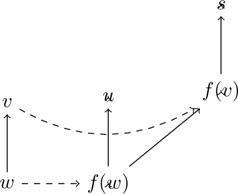
Example 2.4. Figure 3 shows a dynamic model \(\mathcal{M}\), where the modal accessibility relation is a function \(f\). If we disregard the modal relation, \(\mathcal{M}\) is the disjoint union of two intuitionistic Kripke models: a model \(\mathcal{N}_0\) rooted at \(w\) and a model \(\mathcal{N}_1\) rooted at \(f(w)\). The modal relation \(f\) then models the transformation of \(\mathcal{N}_0\) into \(\mathcal{N}_1\).
Suppose \(p \in \mathsf{Prop}\) and \(V\) is the valuation of \(\mathcal{M}\) such that \(p \not \in V(s)\). We claim that \(\mathcal{M}, v \models \larger[-1.5]\square\neg p\). Note that since \(p \not \in V(s)\) and \(V\) is monotone in \(\leq\), also \(p \not \in V(f(v))\). Therefore, \(\mathcal{M}, f(v) \models \neg p\). Since \(f(v)\) is the only modal successor of \(v\) and there are no (proper) intuitionistic successors of \(v\), \(\mathcal{M}, v \models \larger[-1.5]\square\neg p\) as claimed. Now suppose that additionally \({p \in V(u)}\). Then \(\mathcal{M}, w \models \larger[-1.5]\square\neg p\) if and only \(\mathcal{M}, f(w) \models \neg p\) and \(\mathcal{M}, f(v) \models \neg p\). The latter has already been confirmed. For the former, however, note that \(p \in V(u)\), implying that \(\mathcal{M}, f(w) \not \models \neg p\) which in turn implies that \(\mathcal{M}, w \not \models \larger[-1.5]\square\neg p\).
Note that the modalities are evaluated using both \(\leq\) and \(R\). This deviates from the evaluation of modalities in classical modal logic where \(w \models \larger[-1.5]\square\varphi\) if and only if for all \(v\) if \(w \mathrel{R}v\), then \(v \models \varphi\), and \(w \models \larger[-1.5]\Diamond\varphi\) if and only if there exists \(v\) with \(w \mathrel{R}v\) and \(v \models \varphi\). This deviation is necessary since the classical truth conditions do not preserve the monotonicity property of intuitionistic logic: if for example \(w \models \larger[-1.5]\square\varphi\) and \(w \leq v\), then there is no reason that \(v \models \larger[-1.5]\square\varphi\), since the modal successors of \(w\) and \(v\) might be unrelated to one another. To understand the importance of this, observe that a semantics without the monotonicity property will not yield a ‘logic’ with the most basic property: closure under substitutions.
Example 2.5. Consider the formula \(p \rightarrow \neg \neg p\) for \(p \in \mathsf{Prop}\). It is easy to check that \(p \rightarrow \neg \neg p\) is valid over the class of dynamic models. Now substitute \(p\) for \(\larger[-1.5]\squareq\) where \({q \in \mathsf{Prop}}\). By using the classical truth conditions, the formula \(\larger[-1.5]\squareq \rightarrow \neg \neg \larger[-1.5]\squareq\) obtained by the substitution is no longer valid. For a counterexample consider a dynamic model consisting of three worlds, say \(w,v\) and \(u\), such that \(w \leq v\) and \(v \mathrel{R}u\). The valuation is given by \(V(w) = V(v) = V(u) = \emptyset\). Then it easily checked that \(w \models \larger[-1.5]\squareq\) (since \(w\) does not have any modal successors) while \(v \not \models \larger[-1.5]\squareq\), since \(v \mathrel{R}u\) and \(u \not \models q\). Since \(v\) has no intuitionistic successor, \(v \models \neg \larger[-1.5]\squareq\), implying that \(w \not \models \neg \neg \larger[-1.5]\squareq\). Consequently \(w \not \models \larger[-1.5]\squareq \rightarrow \neg \neg \larger[-1.5]\squareq\).
By using the intuitionistic truth conditions for the modalities instead, monotonicity of the semantics is preserved, as illustrated in the following lemma.
Lemma 2.5 (Monotonicity). Let \(\mathcal{M}=(W, \leq, R, V)\) be a dynamic model, \(w,v \in W\) and \(\varphi\) a formula. If \(w \leq v\) and \(\mathcal{M}, w \models \varphi\), then \(\mathcal{M},v \models \varphi\).
Proof. The proof is by induction on the structure of \(\varphi\). The base cases as well as the cases where \(\varphi = \psi \ast \chi\) for \(\ast \in \{\wedge, \vee, \rightarrow\}\) are covered in Lemma 2.2. Suppose \(\varphi = \larger[-1.5]\square\psi\) and \(\mathcal{M},w \models \larger[-1.5]\square\psi\). Then for all \(u_0, u_1 \in W\) if \(w \leq u_0 \mathrel{R}u_1\), then \(\mathcal{M},u_1 \models \psi\). Suppose \(v \leq v' \mathrel{R}u\) for \(v',u \in W\). Since \(v \geq w\) also \(v' \geq w\) and hence \(w \leq v' \mathrel{R}u\). Hence \(\mathcal{M},u \models \psi\) and therefore \(\mathcal{M},v \models \larger[-1.5]\square\psi\). The case for \(\varphi = \larger[-1.5]\Diamond\psi\) is similar. ◻
In the definition of a dynamic model the intuitionstic order \(\leq\) and the modal relation \(R\) are unrelated to one another. We now turn our attention to confluence conditions: interaction principles between \(\leq\) and \(R\) that will be of recurring importance in this thesis. We give a general definition.
Definition 2.19. Let \((X, \leq_X)\) and \((Y, \leq_Y)\) be partially ordered sets and \(R \subseteq X \times Y\) a binary relation between \(X\) and \(Y\). Then
\(R\) is forth-up confluent* (for \((\leq_X, \leq_Y)\)) if for all \(x,x' \in X\) and all \(y \in Y\) it holds that whenever \(x \leq_X x'\) and \(x \mathrel{R}y\), there exists \(y' \in Y\) with \(y \leq_Y y'\) and \(x' \mathrel{R}y'\).*
\(R\) is forth-down confluent* (for \((\leq_X, \leq_Y)\)) if for all \(x,x' \in X\) and \(y \in Y\) it holds that whenever \(x' \leq_X x\) and \(x \mathrel{R}y\), there exists \(y' \in Y\) with \(y' \leq_Y y\) and \(x' \mathrel{R}y'\).*
\(R\) is triangle confluent* (for \((\leq_X, \leq_Y)\)) if for all \(x,x' \in X\) and \(y \in Y\) it holds that whenever \(x \leq_X x'\) and \(x' \mathrel{R}y\), we have \(x \mathrel{R}y\).*
\(R\) is back-up confluent* (for \((\leq_X, \leq_Y)\)) if for all \(x \in X\) and \(y,y' \in Y\) it holds that whenever \(x \mathrel{R}y\) and \(y \leq_Y y'\), there exists \(x' \in X\) with \(x \leq_X x'\) and \(x' \mathrel{R}y'\).*
\(R\) is back-down confluent* (for \((\leq_X, \leq_Y)\)) if for all \(x \in X\) and \(y,y' \in Y\) it holds that whenever \(x \mathrel{R}y\) and \(y' \leq_{\mathcal{Y}} y\), there exists \(x' \in X\) with \(x' \leq_{\mathcal{X}} x\) and \(x' \mathrel{R}y'\).*
See Figure 4 for a depiction of the different confluence conditions.

We will usually consider dynamic models \(\mathcal{M}=(W, \leq, R, V)\) where \(R\) satisfies some confluence condition C for \((\leq, \leq)\). In this case, we simply call \(R\) C-confluent. However, we will also study confluent relations between different posets in Chapter [c: bi-int ml new] and Chapter 6.
One reason why we are interested in confluence conditions is that in forth-up and forth-down confluent dynamic models, the intuitionistic truth conditions for the modalities coincide with the classical truth conditions; the latter can thus be used for convenience. Other reasons will be presented in later chapters. The following is proven in [49].
Lemma 2.6. Let \(\mathcal{M}=(W, \leq, R, V)\) be a dynamic model, \(w \in W\) and \(\varphi\) a formula.
If \(R\) is forth-up confluent, then \(\mathcal{M}, w \models \larger[-1.5]\Diamond\varphi\) if and only if there exists \(v \in W\) with \(w \mathrel{R}v\) and \(\mathcal{M}, v \models \varphi\).
If \(R\) is forth-down confluent, then \(\mathcal{M}, w \models \larger[-1.5]\square\varphi\) if and only if for all \(v \in W\) if \(w \mathrel{R}v\), then \(\mathcal{M}, v \models \varphi\).
Proof sketch.. 1. Suppose \(R\) is forth-up confluent. The direction from left-to-right is trivial. For the direction from right-to-left, suppose there exists \(v \in W\) with \(w \mathrel{R}v\) and \(\mathcal{M}, v \models \varphi\). If \(w \leq u\), then by forth-up confluence there exists \(v'\) with \(v \leq v'\) and \(u \mathrel{R}v'\). By monotonicity \(\mathcal{M},v' \models \varphi\). Hence \(\mathcal{M}, w \models \larger[-1.5]\Diamond\varphi\). The reasoning for 2. is similar. ◻
Corollary 2.1. If \(\mathcal{M}=(W, \leq, R,V)\) is a dynamic model, \(w \in W\), \(\varphi\) a formula and \(R\) is triangle confluent, then \(\mathcal{M}, w \models \larger[-1.5]\square\varphi\) if and only if for all \(v \in W\) if \(w \mathrel{R}v\), then \(\mathcal{M}, v \models \varphi\).
Proof. Note that \(R\) being triangle confluent implies that \(R\) is forth-down confluent. ◻
We are also interested in dynamic models which satisfy certain frame conditions.
Definition 2.20. A dynamic model \(\mathcal{M}=(W, \leq, R, V)\) is called
**reflexive* if \(w \mathrel{R}w\) holds for all \(w \in W\).*
**transitive* if \(w \mathrel{R}v\) and \(v \mathrel{R}u\) imply \(w \mathrel{R}u\) for all \(w,v, u \in W\).*
**symmetric* if \(w \mathrel{R}v\) implies \(v \mathrel{R}w\) for all \(w,v \in W\).*
**serial* if \(dom(R) = W\).*
an S4 model* if \(R\) is reflexive and transitive.*
an S5 model* if \(R\) is an equivalence relation.*
**(total) functional* if \(R\) is a (total) partial function.*
In Chapter 5 and Chapter 6 we will study intuitionistic linear temporal logic, where formulas are evaluated over dynamic models which are total functional. The following lemma is straightforward to check, since in total functional models every world has a unique modal successor. The proof is omitted.
Lemma 2.7. Let \(\mathcal{M}=(W, \leq, f, V)\) be a total functional model. Then the following are equivalent.
\(f\) is forth-up confluent.
\(f\) is forth-down confluent.
\(f\) is monotone in \(\leq\), i.e. for all \(w,v \in W\): \(w \leq v \text{ implies } f(w) \leq f(v)\).
Given this lemma, we will call total functional models which are forth-up or forth-down confluent simply forward confluent.
2.5 Fixed Point Operators↩︎
Intuitionistic dynamic logics are extensions of intuitionistic modal logics with fixed point operators. Intuitively, fixed point operators express infinite statements, such as ‘in all future time steps, \(\varphi\) is true’. In this section we briefly explain why such operators are called fixed point operators. Strictly speaking, the theory explained in this section is not needed for understanding the rest of the thesis. However, we believe that it is informative to understand the concept of a fixed point operator, as it relates the presented logics to one another and also to other modal fixed point logics. We do not give a general definition, but instead explain the concept with an example.
Consider a dynamic model of the form \(\mathcal{M}=(W, \leq, R, V)\), where \(R\) is triangle confluent. Consider the language extending \(\mathcal{L}_\mathsf{IPL}\) by the modality \(\larger[-1.5]\square\) as well as a unary operator \(\ooalign{\larger[-1.5]\square\cr \hidewidth\raise.035ex* \mkern 1.12mu\cr}\) which is characterized semantically as \(\mathcal{M}, w \models \ooalign{\larger[-1.5]\square\cr \hidewidth\raise.035ex* \mkern 1.12mu\cr}\varphi\) if and only if for all \(v \in W\) if \(w \mathrel{R}^* v\), then \(\mathcal{M}, v \models \varphi\) where \(R^*\) is the reflexive transitive closure of \(R\). In other words, \(\ooalign{\larger[-1.5]\square\cr \hidewidth\raise.035ex* \mkern 1.12mu\cr}\varphi\) is true at \(w\) if \(\varphi\) is true in any world \(v\) reachable from \(w\) over finitely many modal steps. Equivalently, \(\ooalign{\larger[-1.5]\square\cr \hidewidth\raise.035ex* \mkern 1.12mu\cr}\varphi\) is equivalent to the infinite conjunction \[\bigwedge_{n < \omega} \larger[-1.5]\square^n \varphi.\] The operator \(\ooalign{\larger[-1.5]\square\cr \hidewidth\raise.035ex* \mkern 1.12mu\cr}\) is called a fixed point operator, namely \(\ooalign{\larger[-1.5]\square\cr \hidewidth\raise.035ex* \mkern 1.12mu\cr}\varphi\) is the greatest fixed point of the propositional function \(x \mapsto \varphi \wedge \larger[-1.5]\squarex\). Let us make precise what is meant by this.
Given a formula \(\varphi\), let \[\llbracket \varphi \rrbracket_\mathcal{M}\mathrel{\vcenter{:}}= \{ w \in W \mid \mathcal{M}, w \models \varphi\}\] be the truth set of \(\varphi\) in \(\mathcal{M}\). Let \(U \subseteq W\) and \(p \in \mathsf{Prop}\) be a proposition not occurring in \(\varphi\). Let \(U^\uparrow\) be the least upwards closed set containing U. Define \(V_U^p: W \longrightarrow \mathcal{P}(\mathsf{Prop})\) as follows: \[V_U^p(w) \mathrel{\vcenter{:}}= \begin{cases} V(w) \cup \{p\} & \text{ if } w\in U^\uparrow \\ V(w) \setminus \{p\} & \text{ otherwise.} \end{cases}\] In other words, the valuation \(V_U^p\) changes the valuation \(V\) by making \(p\) true at the worlds in \(U^\uparrow\) and nowhere else. For any other proposition \(q\), \(q \in V(w)\) if and only if \(q \in V_U^P(w)\). Let \(\mathcal{M}_U^p\) denote the dynamic model \((W, \leq, R, V_U^p)\). Now consider the formula \(\psi = \varphi \wedge \larger[-1.5]\squarep\). This formula induces a function \(f_\psi: \mathcal{P}(W) \longrightarrow \mathcal{P}(W)\) given by \[U \mapsto \llbracket \varphi \wedge \larger[-1.5]\squarep\rrbracket_{\mathcal{M}_U^p}.\]
Given a function \(S: \mathcal{P}(W) \longrightarrow \mathcal{P}(W)\), a fixed point of \(S\) is a subset \(U \subseteq W\) such that \(S(U) = U\). Moreover, \(U\) is the greatest fixed point of \(S\) if for any other fixed point \(U'\) of \(S\) holds that \(U' \subseteq U\) and \(U\) is the least fixed point of \(S\) if for any other fixed point \(U'\) of \(S\) holds that \(U \subseteq U'\). If \(S\) is monotone on \(\mathcal{P}(W)\), meaning that whenever \(U \subseteq U'\) we have \(S(U) \subseteq S(U')\), then the Knaster–Tarski Theorem [50] guarantees that \(S\) has a least and a greatest fixed point.
It is not hard to check that the function \(f_\psi\) is monotone on \(\mathcal{P}(W)\): we have \(\llbracket \varphi \wedge \larger[-1.5]\squarep \rrbracket_{\mathcal{M}} = \llbracket \varphi \rrbracket_\mathcal{M}\cap \llbracket {\larger[-1.5]\squarep} \rrbracket_\mathcal{M}\). Since \(p\) does not occur in \(\varphi\), for any \(U \subseteq U'\), \(\llbracket \varphi \rrbracket_{\mathcal{M}_U^p} = \llbracket \varphi \rrbracket_{\mathcal{M}_{U'}^p}\). Furthermore, clearly \(\llbracket \larger[-1.5]\squarep \rrbracket_{\mathcal{M}_U^p} \subseteq \llbracket \larger[-1.5]\squarep \rrbracket_{\mathcal{M}_{U'}^p}\). Hence \(f_\psi(U) \subseteq f_\psi(U')\). By the Knaster–Tarski Theorem \(f_\psi\) has a greatest fixed point \(U\). One can now show that the greatest fixed point of \(f_\psi\) is exactly the set \(\llbracket \ooalign{\larger[-1.5]\square\cr \hidewidth\raise.035ex* \mkern 1.12mu\cr}\varphi \rrbracket_\mathcal{M}\); for a proof, see [26]. This is the precise meaning behind the statement that \(\ooalign{\larger[-1.5]\square\cr \hidewidth\raise.035ex* \mkern 1.12mu\cr}\varphi\) is the greatest fixed point of the function \(x \mapsto \varphi \wedge \larger[-1.5]\squarex\).
This construction is not dependent on \(\psi\). For any formula \(\gamma\) we can consider the function \(f_\gamma\) induced by \(\gamma\) and if \(f_\gamma\) is monotone, then there exist the least and greatest fixed points. A defining property of all intuitionistic dynamic logics studied in this thesis is that they are extensions with fixed point operators for specific functions. This is not a necessary restriction; instead we could extend the language of \(\mathsf{IML}\) by operators \(\mu\) and \(\nu\) which are applicable to any formula and define the truth set of a formula \(\mu x. \varphi\) as the least fixed point of the function \(f_\varphi\) induced by \(\varphi\) and similarly, \(\nu x. \varphi\) as the greatest fixed point.5 This results in an expressive logical system which is capable of expressing least and greatest fixed points of every monotone function, as opposed to only some. This logic is called intuitionistic modal \(\mu\)-calculus, see Pacheco [30]. For an introduction to modal fixed point logics in general, we refer the reader to the excellent article about the classical modal \(\mu\)-calculus by Stirling [13].
2.6 Historical Remarks↩︎
We finish this chapter by providing a brief historical overview of intuitionistic logic and intuitionistic modal logic.
2.6.1 Intuitionism and Intuitionistic Logic↩︎
The origin of intuitionistic logic goes back to intuitionism, one of the main positions in philosophy of mathematics developed by Dutch mathematician Brouwer [51]. Classical mathematics (at least implicitly) assumes an objective notion of truth: every well-formed mathematical statement such as ‘\(2+2= 4\)’ is either true or false. A common interpretation in philosophy is that truth is a relationship between language and reality [52]. For example, the sentence ‘Young Boys is the best football club in Bern’ is true due to the objective reality regarding football clubs in Bern. But what is the objective reality of the statement ‘\(2+2 = 4\)’ which is regarded to be true in mathematics? The realist position, which originates in the work of Plato, claims that there are objectively existing mathematical objects, such as natural numbers. In other words, there exists a universe of mathematical objects and the statement ‘\(2+2 = 4\)’ expresses the objective reality in this universe and is thus true. Intuitionism rejects the realist position and instead claims that mathematics is a mental activity and mathematical objects exist insofar they have been constructed in the mind of the mathematician. Similarly, proofs are mental constructions and a mathematical statement is true insofar it has been proven. As a consequence, intuitionism rejects indirect proofs which are often used in classical mathematics. For example, an existential statement \(\exists x. \varphi(x)\) is typically proven in classical mathematics by deriving a contradiction from \(\forall x. \neg \varphi(x)\). But such an indirect proof does not result in the construction of an object \(c\) which satisfies \(\varphi(c)\). Instead the indirect proof assumes that the statement \(\exists x. \varphi(x)\) is either true or false, thus deriving a contradiction from its negation \(\forall x. \neg \varphi(x)\) means that \(\exists x. \varphi(x)\) must be true. In intuitionistic mathematics, such an existential statement is proven constructively by constructing the object \(c\) and providing a constructive proof of \(\varphi(c)\). Negations of statements are also treated differently in intuitionistic mathematics. A proof of \(\neg \varphi\) is a proof that \(\varphi\) cannot be proven. Under this interpretation the law of excluded middle does not hold: in classical mathematics \(p \vee \neg p\) is always true since either \(p\) is true or \(p\) is false, in which case \(\neg p\) is true; in intuitionistic mathematics any statement \(p\) is either proven or not proven, but the lack of a proof for \(p\) does not imply that \(p\) cannot be proven, but rather that no proof for \(p\) has been constructed so far. Thus if \(p\) formalizes any unresolved mathematical conjecture, such as the Goldbach conjecture, there is no proof of \(p \vee \neg p\) and so the law of excluded middle fails. This example shows that intuitionistic mathematics uses different logical reasoning principles than classical mathematics. In 1930, Brouwer’s student Heyting isolated the acceptable reasoning principles of intuitionistic mathematics in a formal logical system, leading to the development of intuitionistic logic [1]–[3]. Since then, intuitionistic logic has developed into arguably one of the most successful logical systems, partly due to the following two reasons. First, it is generally accepted that intuitionistic logic succeeded in capturing intuitionistic reasoning and has thus fulfilled its philosophical purpose. Second, alternative interpretations of intuitionistic logic have emerged, which deviate from the original interpretation regarding intuitionism. Among those are interpretations based on computation, topology or information. For example, the Curry–Howard isomorphism relates, roughly speaking, proofs (in some formal proof system for intuitionistic logic) with programs (in some formal model of computation), illustrating a close connection between intuitionistic proofs and computation [53]. This close relation is also illustrated by the fact that many foundational systems for computer science are based on intuitionistic logic [46]. The interpretation of intuitionistic logic guiding this thesis is based on information. As outlined in Chapter 1, we consider intuitionistic logic as a logic to reason about information and information change. This interpretation goes back to Kripke [5], who introduced intuitionistic Kripke models for intuitionistic logic in 1965. As we have seen, these models can be regarded as information orderings and the evaluation of implications as expressing consequences of gaining information. Originally, Kripke provided an interpretation of his semantics as a way to capture the intuitionistic idea that mathematical statements are true if proven and false if proven to be unprovable. The worlds \(w\) of an intuitionistic Kripke model are thought to be information states containing all mathematical theorems which have been proven up to a certain time point. If \(w \leq v\), then \(v\) is thought of as an information state at a later time point obtained by adding more theorems that have been proven in the meantime. If \(w \not \models \varphi\), then \(\varphi\) is not thought to be refuted, but simply to not (yet) been proven. The truth relation should thus be understood as expressing whether a formula has been proven at this point or not. If \(w \models \neg \varphi\), then \(\varphi\) has been proven to be unprovable, implying that for any extension of \(w\), \(\varphi\) cannot be true. Kripke semantics thus provide an intuitive interpretation of intuitionistic logic and are furthermore natural to work with mathematically. However, it should be noted that they are not entirely satisfactory from the point of view of intuitionism: the interpretation of formulas on Kripke models does not refer to the notion of proof directly nor to the idea of constructions; moreover while we have seen that the proof systems of intuitionistic logic presented in Section 2.3 are sound and complete with respect to the class of Kripke models, the completeness proofs require a classical meta theory and are thus not intuitionistically acceptable [7].
For an introduction to intuitionism, we refer the reader to [54]. For a detailed account of the history of intuitionism and constructivism, see [55]. For a detailed introduction to the mathematical theory of intuitionistic logic, see [45], [46].
2.6.2 Intuitionistic Modal Logic↩︎
The modern origin of modal logic arguably goes back to the seminal work of Lewis [56] in 1918, who studied logics of strict implications. After the development of intuitionistic logic by Heyting, both logics were studied independently for several decades. The earliest combination of intuitionistic logic and modal logic is found in the work of Fitch [6] in 1948; however, it was the invention of Kripke semantics for modal logic [57] and for intuitionistic logic [5] by Kripke which laid the foundation for studying intuitionistic modal logic. In the 1980’s, Plotkin and Stirling [58], Ewald [59] and Fischer-Servi [60] independently introduced birelational semantics for intuitionistic modal logic by combining the two types of Kripke models, resulting in the development of the structures that we call dynamic models in this thesis. What followed was the development of a sheer bewildering amount of different intuitionistic modal logics, which differ semantically by the confluence conditions imposed on the dynamic models used for their evaluation. Roughly, these logics fall into two camps: constructive modal logics such as the systems introduced by Fitch [6] and Wijesekera [61] built for modelling computational aspects such as staged computation [11], and intuitionistic modal logics such as the systems by Fischer-Servi [60] and Plotkin and Stirling [58] aimed at capturing an intuitionistic meta reading of modalities and Kripke semantics. In his influential PhD thesis, Simpson [7] set up six criteria that an intuitionistic modal logic should satisfy to be classified as ‘intuitionistic’; one criteria is that there should be an intuitionistically comprehensible explanation of the modalities [7]. Simpson achieves this by providing a translation of intuitionistic modal logic into intuitionistic first-order logic - akin to the translation of modal logic into classical first-order logic - which can then be used as a formalized meta theory. The resulting logic turns out to be \(\mathsf{IK}\), which is semantically obtained by considering all validities over dynamic models satisfying forth-up and back-up confluence.
The restriction to dynamic models satisfying confluence conditions substantially increases the mathematical difficulty of the resulting logics. For example, the logic \(\mathsf{IS4}\) - an intuitionistic version of the modal logic \(\mathsf{S4}\) which satisfies the six criteria posed by Simpson - has only recently been proven to be decidable [62] and the presented proof is highly non-trivial. On the other hand, weaker logics obtained by either not considering any confluence conditions or by considering a restricted language behave more similar to classical modal logics and are generally easier to deal with, see e.g. [25].
3 Intuitionistic Master Modality↩︎
3.1 Introduction↩︎
This chapter introduces a simple intuitionistic dynamic logic called intuitionistic master modality (\(\mathsf{IM}\)). The language of \(\mathsf{IM}\) extends \(\mathcal{L}_\mathsf{IPL}\) by the modality \(\larger[-1.5]\square\) and the fixed point operator \(\ooalign{\larger[-1.5]\square\cr \hidewidth\raise.035ex* \mkern 1.12mu\cr}\) called the master modality, which we encountered in Section 2.5. The modality \(\larger[-1.5]\Diamond\) is not present in the language. Intuitively, \(\ooalign{\larger[-1.5]\square\cr \hidewidth\raise.035ex* \mkern 1.12mu\cr}\varphi\) expresses that \(\varphi\) is true in any world of a dynamic model reachable from the current world over a finite (but arbitrary) number of modal steps. Thus \(\ooalign{\larger[-1.5]\square\cr \hidewidth\raise.035ex* \mkern 1.12mu\cr}\varphi\) is true if \(\larger[-1.5]\square^n \varphi\) is true for any natural number \(n\) and it is characterized as the greatest fixed point of the propositional function \(x \mapsto \varphi \wedge \larger[-1.5]\squarex\). Given the interpretation that intuitionistic modal logic reasons about information updates, a formula \(\ooalign{\larger[-1.5]\square\cr \hidewidth\raise.035ex* \mkern 1.12mu\cr}\varphi\) expresses that \(\varphi\) remains true under any number of information updates. The goal of this chapter is to study the mathematical theory of \(\mathsf{IM}\); in particular the expressivity of its language and its proof theory.
To the best of our knowledge, this work constitutes the first mathematical investigation of \(\mathsf{IM}\). It is worth noting, however, that a multi-modal variant of \(\mathsf{IM}\), known as intuitionistic common knowledge logic (\(\mathsf{ICK}\)), was previously introduced and studied by Jäger and Marti. [25], [27]. Classical versions of \(\mathsf{IM}\) have also been studied extensively, see e.g. [63]. Originally, one of our main motivations to study \(\mathsf{IM}\) was the interpretation of \(\mathsf{IM}\) as an intuitionistic linear temporal logic. To that end formulas are evaluated on dynamic models where the modal relation is a function modeling time. Such models are called functional models. In difference to stronger temporal logics such as \(\mathsf{iLTL}\), which will be studied in Chapter 5, the functional models of \(\mathsf{IM}\) do not satisfy any confluence conditions. The modality \(\larger[-1.5]\square\) is then interpreted as a temporal ‘next’ operator and the master modality as a temporal ‘henceforth’, i.e. \(\ooalign{\larger[-1.5]\square\cr \hidewidth\raise.035ex* \mkern 1.12mu\cr}\varphi\) is true if \(\varphi\) is true in any future time step. As it turns out, the language of \(\mathsf{IM}\) is not expressive enough for such an interpretation. Namely, the set of valid formulas over functional models coincides with the set of valid formulas of arbitrary dynamic models, implying that the restriction to functions does not have an impact on the logic. This discourages an interpretation of \(\mathsf{IM}\) as temporal logic. Nevertheless, \(\mathsf{IM}\) remains a relevant logical system in its own right: \(\mathsf{IM}\) is an interesting case study for applying techniques from the study of classical modal fixed point logics to the intuitionistic realm. This is due to the relatively simple mathematical theory of \(\mathsf{IM}\), caused by the lack of meaningful confluence conditions imposed on its dynamic models. Moreover, \(\mathsf{IM}\) serves as the stepping stone to investigate other, more expressive, intuitionistic dynamic logics, such as intuitionistic common knowledge logic which will be studied in Chapter 4 or intuitionistic versions of propositional dynamic logic (\(\mathsf{PDL}\)). The techniques developed to investigate \(\mathsf{IM}\) can be applied or adapted for more complex logics, as illustrated in Chapter 4 where much of the proof theoretic work for \(\mathsf{IM}\) is applied successfully to \(\mathsf{ICK}\).
The next section introduces the syntax and semantics of \(\mathsf{IM}\). The semantics is given in terms of dynamic models, where we consider three classes: the class of all dynamic models, the class of functional dynamic models and the class of dynamic models which are triangle confluent. Regarding expressivity, we prove that the language of \(\mathsf{IM}\) cannot distinguish between all three classes of models, in the sense that they all produce the same set of validites (see Theorem 3.1). Afterwards we turn to proof theory and introduce a sound and complete axiomatization for \(\mathsf{IM}\). The completeness proof is by a standard canonical model construction. Our proof is similar to the completeness proof for classical common knowledge logic presented in [64], highlighting the straightforward adaptation of classical techniques to \(\mathsf{IM}\). Completeness for a multi-modal version of \(\mathsf{IM}\) was already established for a different axiomatization by Marti in his PhD thesis [26], and the presented proof closely follows Marti’s proof. The remaining sections study a sequent calculus for \(\mathsf{IM}\). Due to the presence of the master modality, our proof systems require a formal counterpart to induction. Instead of using an induction rule as is done in [25], we instead employ non-wellfounded and cyclic proofs. First, we give a brief introduction to such proof formalisms and then introduce the cyclic calculus \(\mathrm{cIM}\) and the non-wellfounded calculus \(\mathrm{nIM}\). The calculus \(\mathrm{nIM}\) is not studied in its own right but used as a tool to establish completeness for \(\mathrm{cIM}\). We prove soundness of \(\mathrm{cIM}\) by an indirect argument and completeness for \(\mathrm{nIM}\) via a proof search argument. It is then shown how to translate non-wellfounded proofs into cyclic proofs, whence establishing completeness for \(\mathrm{cIM}\) as well. The presented proof search method is quite robust, which will be illustrated by showing how to obtain dynamic, triangle and functional countermodels from a failed proof search, which requires only minor adjustments to the overall argument. This will also provide an alternative proof of Theorem 3.1 using proof theoretic means.
3.2 Syntax and Semantics↩︎
The language \(\mathcal{L}_\mathrm{IM}\) of \(\mathsf{IM}\) extends \(\mathcal{L}_\mathsf{IPL}\) by the modal operator \(\larger[-1.5]\square\) and the fixed point operator \(\ooalign{\larger[-1.5]\square\cr \hidewidth\raise.035ex* \mkern 1.12mu\cr}\) called the master modality. Formulas of \(\mathcal{L}_\mathrm{IM}\) are given by the following grammar in Backus–Naur form: \[\varphi ::= \bot \, \lvert \, p \, \lvert \, \varphi \wedge \varphi \, \lvert \, \varphi \vee \varphi \, \lvert \, \varphi \rightarrow \varphi \, \lvert \, \larger[-1.5]\square\varphi \, \lvert \, \ooalign{\larger[-1.5]\square\cr \hidewidth\raise.035ex* \mkern 1.12mu\cr}\varphi.\] where \(p \in \mathsf{Prop}\). As before we write \(\varphi \in \mathcal{L}_\mathrm{IM}\) to denote that \(\varphi\) is a \(\mathcal{L}_\mathrm{IM}\)-formula and we use the same conventions for the brackets and the notation as introduced for \(\mathcal{L}_\mathsf{IPL}\).
Definition 3.1. The closure* \(\mathsf{Cl}(\varphi)\) of a formula \(\varphi\) is defined by induction on \(\varphi\) as follows.*
\(\mathsf{Cl}(\bot) = \{\bot\}\)
\(\mathsf{Cl}(p) = \{ p \}\) for \(p \in \mathsf{Prop}\)
\(\mathsf{Cl}(\varphi \ast \psi) = \mathsf{Cl}(\varphi) \cup \mathsf{Cl}(\psi) \cup \{ \varphi \ast \psi\}\) for \(\ast \in \{\wedge, \vee, \rightarrow\}\)
\(\mathsf{Cl}(\larger[-1.5]\square\varphi) = \mathsf{Cl}(\varphi) \cup \{\larger[-1.5]\square\varphi\}\)
\(\mathsf{Cl}(\ooalign{\larger[-1.5]\square\cr \hidewidth\raise.035ex* \mkern 1.12mu\cr}\varphi) = \mathsf{Cl}(\varphi) \cup \{\ooalign{\larger[-1.5]\square\cr \hidewidth\raise.035ex* \mkern 1.12mu\cr}\varphi, \larger[-1.5]\square\ooalign{\larger[-1.5]\square\cr \hidewidth\raise.035ex* \mkern 1.12mu\cr}\varphi\}\)
Given a set \(\Gamma\) of formulas, the closure* \(\mathsf{Cl}(\Gamma)\) of \(\Gamma\) is defined by \[\mathsf{Cl}(\Gamma):= \bigcup_{\varphi\in\Gamma}\mathsf{Cl}(\varphi).\] A set of formulas \(\Gamma\) is closed if \(\Gamma = \mathsf{Cl}(\Gamma)\).*
The following lemma is established by a straightforward induction on the structure of \(\varphi\). The proof is omitted.
Lemma 3.1. For any formula \(\varphi\), the closure \(\mathsf{Cl}(\varphi)\) is finite.
The complexity of a formula is defined as follows.
Definition 3.2. The complexity* \(c(\varphi)\) of a formula \(\varphi\) is defined by induction on \(\varphi\) as follows.*
\(c(\bot) = c(p) = 0\)
\(c(\varphi \ast \psi) = c(\varphi) + c(\psi) +1\) for \(\ast \in \{\wedge, \vee, \rightarrow\}\)
\(c(\larger[-1.5]\square\varphi) = c(\ooalign{\larger[-1.5]\square\cr \hidewidth\raise.035ex* \mkern 1.12mu\cr}\varphi) = c(\varphi) + 1\)
Given a finite set of formulas \(\Gamma\), the complexity* \(c(\Gamma)\) of \(\Gamma\) is defined as \[c(\Gamma) = \sum_{\varphi \in \Gamma}c(\varphi).\]*
We will evaluate formulas of \(\mathcal{L}_\mathsf{IM}\) over three classes of dynamic models: the class of all dynamic models (see Definition 2.17), the class of functional models (see Definition 2.20), and the class of triangle models, which are defined as follows.
Definition 3.3. A triangle model* is a dynamic model \(\mathcal{M}=(W, \leq, R, V)\) where \(R\) is triangle confluent.6*
By Corollary 2.1 we can use the classical truth conditions for the modalities when evaluating formulas over triangle models, but in order to obtain monotonicity we shall use the intuitionistic truth conditions for modalities when evaluating formulas over dynamic and functional models. Thus we introduce two truth relations \(\models\) and \(\models_t\).
For any binary relation \(S\), let \(S^*\) denote the reflexive transitive closure of \(S\). Given a dynamic model \(\mathcal{M}=(W,\leq,R,V)\), let \(\tilde{R}\) denote the composition \(R \circ {\leq}\), i.e. \(w \mathrel{\tilde{R}} v\) holds if and only if there exists \(u \in W\) with \(w \leq u\) and \(u \mathrel{R}v\). Note that, since \(\leq\) is reflexive, \(w \mathrel{(\tilde{R})^*} v\) holds if and only if there exist a natural number \(n\) and worlds \(u_0, \ldots, u_{2n}\) such that \(u_0 = w\), \(u_{2n} = v\) and for all \(0 \leq i < n\) both \(u_{2i} \leq u_{2i+1}\) and \(u_{2i+1} \mathrel{R}u_{2(i+1)}\) hold.
Definition 3.4. The truth relation* \(\models\) between worlds of a dynamic (functional) model \(\mathcal{M}=(W, \leq, R, V)\) and formulas is defined by extending Definition 2.7 with the following clauses, where \(w \in W\).*
| \(\mathcal{M},w \models \larger[-1.5]\square\varphi\) | iff | for all \(v \in W\) if \(w \mathrel{\tilde{R}} v\), then \(\mathcal{M},v \models \varphi\), |
| \(\mathcal{M},w \models \ooalign{\larger[-1.5]\square\cr \hidewidth\raise.035ex* \mkern 1.12mu\cr}\varphi\) | iff | for all \(v \in W\) if \(w \mathrel{(\tilde{R})^*} v\), then \(\mathcal{M},v \models \varphi\). |
If \(\mathcal{M}, w \models \varphi\), then \(\varphi\) is called true* at \(w\).*
A formula \(\varphi\) is satisfiable over the class of dynamic (functional) models if there exists a dynamic (functional) model \(\mathcal{M}=(W, \leq, R, V)\) and a world \(w \in W\) such that \({\mathcal{M},w \models \varphi}\), and unsatisfiable otherwise. The formula \(\varphi\) is valid over the class of dynamic (functional) models if for any dynamic (functional) model \(\mathcal{M}=(W, \leq, R, V)\) and any world \(w \in W\) holds that \(\mathcal{M},w \models \varphi\), and falsifiable otherwise.
Lemma 3.2 (Monotonicity of \(\models\)). Let \(\varphi\in \mathcal{L}_\mathrm{IM}\) and let \({\mathcal{M}= (W, \leq, R, V)}\) be a dynamic (functional) model with \(w,v \in W\). If \(w \leq v\) and \(\mathcal{M},w \models \varphi\), then \(\mathcal{M},v \models \varphi\).
Proof. Recall that every functional model is a dynamic model. Therefore it suffices to prove the lemma for dynamic models. Let \({\mathcal{M}= (W, \leq, R, V)}\) be a dynamic model with \(w,v \in W\) and suppose that \(w \leq v\). We proceed by induction on the structure of \(\varphi\). Each case apart from \(\varphi = \ooalign{\larger[-1.5]\square\cr \hidewidth\raise.035ex* \mkern 1.12mu\cr}\psi\) is covered in Lemma 2.2 and Lemma 2.5.
Suppose \(\mathcal{M},w \models \ooalign{\larger[-1.5]\square\cr \hidewidth\raise.035ex* \mkern 1.12mu\cr}\psi\). Then for all \(u \in W\) with \(w \mathrel{(\tilde{R})^*} u\) holds that \(\mathcal{M},u \models \psi\). Suppose \(v \mathrel{(\tilde{R})^*} u\) for some \(u \in W\). Then there exist \(u_0, \ldots, u_{2n} \in W\) with \(u_0 = v\), \(u_{2n} = u\) and for all \(0 \leq i < n\), \(u_{2i} \leq u_{2i+1}\) and \(u_{2i+1} \mathrel{R}u_{2(i+1)}\). Therefore, \(v \leq u_1\) and since \(w \leq v\), also \(w \leq u_1\). Hence \(w \mathrel{(\tilde{R})^*} u\) and so \(\mathcal{M},u \models \psi\). We conclude that \(\mathcal{M},v \models \ooalign{\larger[-1.5]\square\cr \hidewidth\raise.035ex* \mkern 1.12mu\cr}\psi\). ◻
Next, we introduce the truth relation \(\models_t\) for evaluating formulas on triangle models.
Definition 3.5. The definition of the truth relation \(\models_t\) between worlds of a triangle model \(\mathcal{M}=(W, \leq, R,V)\) and formulas is defined by extending Definition 2.7 with the following clauses, where \({w \in W}\).
| \(\mathcal{M},w \models_t \larger[-1.5]\square\varphi\) | iff | for all \(v \in W\) if \(w \mathrel{R} v\), then \(\mathcal{M},v \models_t \varphi\), |
| \(\mathcal{M},w \models_t \ooalign{\larger[-1.5]\square\cr \hidewidth\raise.035ex* \mkern 1.12mu\cr}\varphi\) | iff | for all \(v \in W\) if \(w \mathrel{R^*} v\), then \(\mathcal{M},v \models_t \varphi\). |
Note that every triangle model \(\mathcal{M}=(W, \leq, R, V)\) satisfies \(R = \tilde{R}\). The monotonicity property for \(\models_t\) follows immediately from Corollary 2.1 and Lemma 3.2.
Lemma 3.3 (Monotonicity of \(\models_t\)). Let \(\varphi\in \mathcal{L}_\mathrm{IM}\) and let \({\mathcal{M}= (W, \leq, R, V)}\) be a triangle model with \(w,v \in W\). If \(w \leq v\) and \(\mathcal{M},w \models_t \varphi\), then \(\mathcal{M},v \models_t \varphi\).
Definition 3.6. Let
\(\mathbf{IM}\) be the set of valid \(\mathcal{L}_\mathrm{IM}\)-formulas over the class of dynamic models.
\(\mathbf{IM_f}\) be the set of valid \(\mathcal{L}_\mathrm{IM}\)-formulas over the class of functional models.
\(\mathbf{IM_t}\) be the set of valid \(\mathcal{L}_\mathrm{IM}\)-formulas over the class of triangle models.
The logic \(\mathbf{IM_f}\) can be interpreted as an intuitionistic version of linear temporal logic, where \(f\) is the function mapping each world to its temporal successor, \(\larger[-1.5]\square\) is interpreted as ‘next’ and \(\ooalign{\larger[-1.5]\square\cr \hidewidth\raise.035ex* \mkern 1.12mu\cr}\) as ‘henceforth’. It makes sense under such an interpretation to assume \(f\) to be a total function. Note that \(\mathbf{IM_f}\) does not validate some of the standard tautologies of linear temporal logic, such as \(\larger[-1.5]\square(p \vee q) \rightarrow (\larger[-1.5]\squarep \vee \larger[-1.5]\squareq)\).
Lemma 3.4. \(\larger[-1.5]\square(p \vee q) \rightarrow (\larger[-1.5]\squarep \vee \larger[-1.5]\squareq) \not \in \mathbf{IM_f}\).
Proof. Consider the functional model \(\mathcal{M}=(W, \leq, f, V)\) depicted in Figure 5, where \(V(w) = V(v) = \emptyset\), \(V(f(w)) = \{p\}\) and \(V(f(v)) = \{q\}\). Note that \(\mathcal{M}, w \models \larger[-1.5]\square(p \vee q)\) since \(\mathcal{M}, f(w) \models p\) and hence \(\mathcal{M}, f(w) \models p \vee q\) and \(\mathcal{M}, f(v) \models q\) and so \(\mathcal{M}, f(v) \models p \vee q\). However, \(\mathcal{M}, w \not \models \larger[-1.5]\squarep\), since \(w \leq v\) and \(\mathcal{M}, f(v) \not \models p\). Similarly, \(\mathcal{M}, w \not \models \larger[-1.5]\squareq\) since \(\mathcal{M}, f(w) \not \models q\). Hence \(\mathcal{M}, w \not \models \larger[-1.5]\squarep \vee \larger[-1.5]\squareq\). ◻
![Figure 5: A (total) functional model falsifying \larger[-1.5]\square(p \vee q) \rightarrow (\larger[-1.5]\squarep \vee \larger[-1.5]\squareq).](/article/2607.13528/_pdflatex/wubnaghy.png "fig:")
We finish this section with the following lemma, stating that every formula valid over the class of dynamic models is also valid over the classes of functional and triangle models. Note that this trivially holds since both functional and triangle models are dynamic models and \(\mathcal{M}, w \models \varphi\) if and only if \(\mathcal{M}, w \models_t \varphi\) for any triangle model \(\mathcal{M}\) and any world \(w\) by Corollary 2.1.
Lemma 3.5. The following hold.
\(\mathbf{IM} \subseteq \mathbf{IM_t}\)
\(\mathbf{IM} \subseteq \mathbf{IM_f}\)
3.3 Expressivity↩︎
This section explores whether the language \(\mathcal{L}_\mathsf{IM}\) can distinguish between the classes of dynamic, functional and triangle models. The main result is Theorem 3.1, stating that all three classes have the same set of valid formulas, i.e. \[\mathbf{IM} = \mathbf{IM_t} = \mathbf{IM_f}.\]
That \(\mathbf{IM} = \mathbf{IM_t}\) is straightforward, and was already observed about the language of \(\mathcal{L}_\mathrm{IM}\) without the master modality in [65]. The following lemma provides a brief proof sketch.
Lemma 3.6. \(\mathbf{IM} = \mathbf{IM_t}\).
Proof sketch. That \(\mathbf{IM} \subseteq \mathbf{IM_t}\) is Lemma 3.5. For the other inclusion let \(\mathcal{M}=(W, \leq, R, V)\) be a dynamic model and define \(\mathcal{M}' = (W, \leq, (R \circ {\leq}), V)\). Clearly, \((R \circ {\leq})\) is triangle confluent and therefore \(\mathcal{M}'\) is a triangle model. We show by induction on the structure of \(\varphi\) that for any \(w \in W\) and any \(\varphi \in \mathcal{L}_\mathrm{IM}\) hold that \[\mathcal{M}, w \models \varphi \text{ iff } \mathcal{M}', w \models_t \varphi\]
The base cases and the cases where the main connective of \(\varphi\) belongs to \(\{\wedge, \vee, \rightarrow \}\) are routine. The cases where \(\varphi = \larger[-1.5]\square\psi\) or \(\varphi = \ooalign{\larger[-1.5]\square\cr \hidewidth\raise.035ex* \mkern 1.12mu\cr}\psi\) then follow immediately from the observation that \(\tilde{R} = (R \circ {\leq})\). Therefore if a formula \(\varphi\) is falsifiable over the class of dynamic models, then there exists a dynamic model \(\mathcal{M}\) and a world \(w\) with \(\mathcal{M}, w \not \models \varphi\), implying that \(\mathcal{M}', w \not \models_t \varphi\). Hence \(\varphi\) is falsifiable over the class of triangle models and so \(\mathbf{IM_t} \subseteq \mathbf{IM}\). ◻
3.3.1 Dynamic and Functional Models↩︎
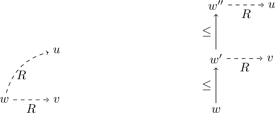
The goal of this subsection is to establish \(\mathbf{IM} = \mathbf{IM_f}\). By Lemma 3.5, \(\mathbf{IM} \subseteq \mathbf{IM_f}\). For the other inclusion, given a formula \(\varphi\) and a dynamic model \(\mathcal{M}\) falsifying \(\varphi\), we have to show how to construct a functional model \(\mathcal{M}'\) falsifying \(\varphi\). The functional model \(\mathcal{M}'\) will be constructed in stages: we start by adding a copy of the world \(w\) of \(\mathcal{M}\) which falsifies \(\varphi\). Then, in later steps, we add copies of worlds of \(\mathcal{M}\) in such a way that the copy of \(w\) satisfies and falsifies the same formulas as \(w\), and the resulting model is functional. The crucial insight is that if a world \(w\) of \(\mathcal{M}\) has multiple modal successors, we can simply add, for each modal successor, a copy of \(w\) as an intuitionistic successor of \(w\) and for each copy one modal successor. Due to the intuitionistic truth conditions, both models then satisfy the same modal formulas. See Figure 6 for an illustration. In order to formalize the construction, we introduce induced structures.
Definition 3.7. Let \(\mathcal{M}=(W, \leq, R, V)\) be a dynamic model. An \(\mathcal{M}\)-induced structure* is a tuple \(\mathcal{I}=(I, \leq_I, R_I, V_I)\) together with a function \(\pi: I \longrightarrow W\) such that the following hold.*
\(I\) is a finite set.
\((I, \leq_I)\) is a poset and if \(x \leq_I y\), then \(\pi(x) \leq \pi(y)\).
\(R_I: I \longrightarrow I\) is a partial function such that if \(R_I(x) = y\), then \(\pi(x) \mathrel{R} \pi(y)\).
\(V_I = V \circ \pi\).
Since we are only interested in falsifying the formula \(\varphi\), it suffices to ensure that the constructed model evaluates formulas in the closure of \(\varphi\) correctly. Therefore the following definition is given relative to a finite and closed set of formulas \(\Sigma\).
Definition 3.8. Let \(\Sigma\) be a closed and finite set of formulas. Let \(\mathcal{M}=(W, \leq, R, V)\) be a dynamic model, \(\langle \mathcal{I}=(I, \leq_I, R_I, V_I), \pi \rangle\) an \(\mathcal{M}\)-induced structure and \(x \in I\).
An \(\rightarrow\)-defect* of \(\mathcal{I}\) is a tuple \((x,\psi \rightarrow \chi)\) where \(x \in I\) and \(\psi \rightarrow \chi \in \Sigma\), such that \(\mathcal{M}, \pi(x) \not \models \psi \rightarrow \chi\), but there does not exist a world \(y \in I\) such that \(y \geq_I x\) and \(\mathcal{M}, \pi(y) \models \psi\) and \(\mathcal{M}, \pi(y) \not \models \chi\).*
A \(\larger[-1.5]\square\)-defect* of \(\mathcal{I}\) is a tuple \((x,\larger[-1.5]\square\psi)\) where \(x \in I\) and \(\larger[-1.5]\square\psi \in \Sigma\), such that \(\mathcal{M}, \pi(x) \not \models \larger[-1.5]\square\psi\) but there does not exists a world \(y \in I\) with \(x \mathrel{( R_I \circ {\leq_I})} y\) and \(\mathcal{M}, \pi(y) \not \models \psi\).*
A \(\ooalign{\larger[-1.5]\square\cr \hidewidth\raise.035ex* \mkern 1.12mu\cr}\)-defect of \(\mathcal{I}\) is a tuple \((x, \ooalign{\larger[-1.5]\square\cr \hidewidth\raise.035ex* \mkern 1.12mu\cr}\psi)\) where \(x \in I\) and \(\ooalign{\larger[-1.5]\square\cr \hidewidth\raise.035ex* \mkern 1.12mu\cr}\psi \in \Sigma\), such that \(\mathcal{M}, \pi(x) \not \models \ooalign{\larger[-1.5]\square\cr \hidewidth\raise.035ex* \mkern 1.12mu\cr}\psi\) but there does not exist a world \(y \in I\) with \(x \mathrel{( R_I \circ {\leq_I})^\ast} y\) and \(\mathcal{M}, \pi(y) \not \models \psi\).
Observe that for any \(\mathcal{M}\)-induced structure \(\mathcal{I}\) and any closed and finite set of formulas \(\Sigma\), there are only finitely many defects, due to \(I\) and \(\Sigma\) being finite.
Suppose \(\mathcal{M}=(W, \leq, R, V)\) is a dynamic model and \(w \in W\) a world such that \(\mathcal{M},w \not \models \varphi\). We are going to construct a functional model \(\mathcal{I}_\omega=(I_\omega, \leq_\omega, R_\omega, V_\omega)\) falsifying \(\varphi\) in stages. To that end let \(\Sigma = \mathsf{Cl}(\varphi)\). We define for each natural number \(n\) an \(\mathcal{M}\)-induced structure \(\mathcal{I}_n\) as well as a first-in-first-out queue \(D\) that stores the defects of \(\mathcal{I}_n\) and we simultaneously prove that \(\mathcal{I}_n\) is an \(\mathcal{M}\)-induced structure. The functional model \(\mathcal{I}_\omega\) is then defined as the limit of the sequence \((\mathcal{I}_n)_{n < \omega}\).
Stage 0: Define the \(\mathcal{M}\)-induced structure \(\langle \mathcal{I}_0 =(I_0, \leq_0, R_0, V_0), \pi_0\rangle\) as follows.
\(I_0 \mathrel{\vcenter{:}}= \{\tilde{x}\}\) where \(\tilde{x}\) is a fresh world not contained in \(W\).
\(\leq_0 \mathrel{\vcenter{:}}= \{(\tilde{x},\tilde{x})\}\).
\(R_0 \mathrel{\vcenter{:}}= \emptyset\).
\(V_0(\tilde{x}) \mathrel{\vcenter{:}}= V(w)\).
\(\pi_0(\tilde{x}) \mathrel{\vcenter{:}}= w\).
To complete stage 0, initialize the queue \(D\) by adding all defects of \(\mathcal{I}_0\) to \(D\) in arbitrary order. It is immediate to check that \(\mathcal{I}_0\) is an \(\mathcal{M}\)-induced structure.
Stage n+1: Suppose \(\langle \mathcal{I}_n =(I_n, \leq_n, R_n, V_n), \pi_n \rangle\) has been defined and \(D\) currently stores the defects of \(\mathcal{I}_n\). We show first how to construct \(\langle \mathcal{I}_{n+1}, \pi_{n+1}\rangle\) depending on the defect at the head of the queue \(D\) and then how to update \(D\).
(\(\rightarrow\)-defects) Suppose the defect at the head of the queue \(D\) is an \(\rightarrow\)-defect \((y, \psi \rightarrow \chi)\). Then \(y \in I_n\), \(\psi \rightarrow \chi \in \Sigma\) and \(\mathcal{M}, \pi_n(y) \not \models \psi \rightarrow \chi\), however there does not exists a world \(y' \in I_n\) with \(y' \geq_n y\) such that \(\mathcal{M}, \pi_n(y') \models \psi\) and \(\mathcal{M}, \pi_n(y') \not \models \chi\). Since \({\mathcal{M}, \pi_n(y) \not \models \psi \rightarrow \chi}\), there exists a world \(u \geq \pi_n(y)\) such that \(\mathcal{M},u \models \psi\) and \(\mathcal{M},u \not \models \chi\). Let \(y'\) be a fresh world not occurring in \(I_n\) or \(W\) and define
\(I_{n+1} \mathrel{\vcenter{:}}= I_n \cup \{y'\}\);
let \(\leq_{n+1}\) be the reflexive transitive closure of \(\leq_n \cup \{(y, y')\}\);
\(R_{n+1} \mathrel{\vcenter{:}}= R_n\);
\(V_{n+1}\) is defined by \[V_{n+1}(z) := \begin{cases} V(u) & \text{if } z=y'\\ V_n(z) & \text{otherwise;}\\ \end{cases}\]
\(\pi_{n+1}\) is defined by \[\pi_{n+1}(z) := \begin{cases} u & \text{if } z= y'\\ \pi_n(z) & \text{otherwise.}\\ \end{cases}\]
To see that \(\mathcal{I}_{n+1}\) is an \(\mathcal{M}\)-induced structure, first note that by induction hypothesis \(I_n\) is a finite set, and therefore \(I_{n+1}\) is a finite set too. Suppose \(x \leq_{n+1} z\). Then either \(x \leq_n z\) which implies by induction hypothesis that \(\pi_n(x) \leq \pi_n(z)\) and thus also \(\pi_{n+1}(x) \leq \pi_{n+1}(z)\), or \(x \leq_n y\) and \(z= y'\), which, by construction and induction hypothesis, implies \(\pi_{n+1}(x) \leq \pi_{n+1}(y) \leq \pi_{n+1}(z)\). That \((I_{n+1}, \leq_{n+1})\) is a poset follows immediately from the induction hypothesis and the construction. Next, \(R_{n+1} = R_n\) by construction and thus, by induction hypothesis, \(R_{n+1}\) is a partial function and if \(R_{n+1}(x) = z\), then \(\pi_{n+1}(x)\mathrel{R}\pi_{n+1}(z)\). If \(x \in I_n\), then \(V_n(x) = V(\pi_n(x))\) by induction hypothesis, so by construction \(V_{n+1}(x) = V(\pi_{n+1}(x))\). Otherwise \(x= y'\) and \(V_{n+1}(x) = V(\pi_{n+1}(x))\) by construction. Thus \(V_{n+1}= V \circ \pi_{n+1}\). Finally, by induction hypothesis \(\pi_n: I_n \longrightarrow W\) is a function. Since \(y'\) is a fresh world, \(\pi_{n+1}:I_{n+1} \longrightarrow W\) is a function as well. Thus \(\langle \mathcal{I}_{n+1}, \pi_{n+1}\rangle\) is an \(\mathcal{M}\)-induced structure.
(\(\larger[-1.5]\square\)-defects) Suppose the defect at the head of the queue \(D\) is a \(\larger[-1.5]\square\)-defect \((y, \larger[-1.5]\square\psi)\). Then \(y \in I_n\), \(\larger[-1.5]\square\psi \in \Sigma\), \(\mathcal{M}, \pi_n(y) \not \models \larger[-1.5]\square\psi\) but there does not exist a world \(y' \in I_n\) with \(y \mathrel{(R_n \circ {\leq_n})} y'\) and \(\mathcal{M}, \pi_n(y') \not \models \psi\). Since \(\mathcal{M}, \pi_n(y) \not \models \larger[-1.5]\square\psi\), there exist worlds \(u_0, u_1 \in W\) with \(\pi_n(y) \leq u_0 \mathrel{R} u_1\) and \(\mathcal{M}, u_1 \not \models \psi\). Let \(y_0, y_1\) be fresh worlds7 not occurring in \(I_n\) or \(W\). Define
\(I_{n+1} \mathrel{\vcenter{:}}= I_n \cup \{y_0, y_1\}\);
let \(\leq_{n+1}\) be the reflexive transitive closure of \(\leq_n \cup \{(y, y_0)\}\);
\(R_{n+1} \mathrel{\vcenter{:}}= R_n \cup \{(y_0,y_1)\}\);
\(V_{n+1}\) is defined by \[V_{n+1}(z) := \begin{cases} V(u_0) & \text{if } z= y_0\\ V(u_1) & \text{if } z= y_1 \\ V_n(z) & \text{otherwise;}\\ \end{cases}\]
\(\pi_{n+1}\) is defined by \[\pi_{n+1}(z) := \begin{cases} u_0 & \text{if } z= y_0\\ u_1 & \text{if } z= y_1 \\ \pi_n(z) & \text{otherwise.}\\ \end{cases}\]
Let us check that \(\mathcal{I}_{n+1}\) is an \(\mathcal{M}\)-induced structure. That \(I_{n+1}\) is finite, \(x \leq_{n+1} y\) implies \(\pi_{n+1}(x) \leq \pi_{n+1}(y)\) and that \((I_{n+1}, \leq_{n+1})\) is a poset follow by similar argument as above. Suppose \(R_{n+1}(x) = z\). Then either \(R_n(x) = z\), which by induction hypothesis implies that \(\pi_n(x) \mathrel{R} \pi_n(y)\) and so \(\pi_{n+1}(x) \mathrel{R} \pi_{n+1}(y)\) by construction, or \(x=y_0\) and \(z = y_1\). In that case we have by construction \(\pi_{n+1}(x) \mathrel{R} \pi_{n+1}(y)\) as well. Moreover, by induction hypothesis and construction, \(R_{n+1}\) is a partial function. That \(V_{n+1} = V \circ \pi_{n+1}\) and that \(\pi_{n+1}\) is a function follow by similar arguments as above.
(\(\ooalign{\larger[-1.5]\square\cr \hidewidth\raise.035ex* \mkern 1.12mu\cr}\)-defects) Suppose the defect at the head of the queue \(D\) is a \(\ooalign{\larger[-1.5]\square\cr \hidewidth\raise.035ex* \mkern 1.12mu\cr}\)-defect \((y, \ooalign{\larger[-1.5]\square\cr \hidewidth\raise.035ex* \mkern 1.12mu\cr}\psi)\). Then \({y \in I_n}\), \(\ooalign{\larger[-1.5]\square\cr \hidewidth\raise.035ex* \mkern 1.12mu\cr}\psi \in \Sigma\), \(\mathcal{M}, \pi_n(y) \not \models \ooalign{\larger[-1.5]\square\cr \hidewidth\raise.035ex* \mkern 1.12mu\cr}\psi\) but there does not exist a world \(y' \in I_n\) with \({y \mathrel{(R_n \circ {\leq_n})^*} y'}\) such that \(\mathcal{M}, \pi_n(y') \not \models \psi\). Since \(\mathcal{M}, \pi_n(y) \not \models \ooalign{\larger[-1.5]\square\cr \hidewidth\raise.035ex* \mkern 1.12mu\cr}\psi\), there exists a world \(u \in W\) with \(\pi_n(y) \mathrel{(R \circ {\leq})^*} u\) and \(\mathcal{M},u \not \models \psi\). Let \(u_0, \ldots, u_{2k} \in W\) such that \(u_0 = \pi_n(y)\), \(u_{2k} = u\) and for all \(0 \leq i < k\) holds that \(u_{2i} \leq u_{2i+1}\) and \(u_{2i+1} \mathrel{R}u_{2(i+1)}\). Observe that \(k > 0\) as by assumption \(\mathcal{M}, \pi_n(y) \models \psi\) (again, some worlds \(u_{2i+1}\) might be identical to \(u_{2i}\)). Let \(y_i\) for \(1 \leq i \leq 2k\) be fresh worlds not occuring in \(I_n\) or \(W\). Define
\(I_{n+1} \mathrel{\vcenter{:}}= I_n \cup \{y_1, \ldots, y_{2k}\}\);
let \(\leq_{n+1}\) be the reflexive transitive closure of \[\leq_n \cup \{(y, y_1)\} \cup \{(y_{2i}, y_{2i+1}) \, \lvert \, 1 \leq i < k\};\]
\(R_{n+1} \mathrel{\vcenter{:}}= R_n \cup \{(y_{2i+1}, y_{2(i+1)}) \, \lvert \, 0 \leq i < k\}\);
\(V_{n+1}\) is defined by \[V_{n+1}(z) \mathrel{\vcenter{:}}= \begin{cases} V(u_i) & \text{if } z= y_i \text{ for } 1 \leq i \leq 2k\\ V_n(z) & \text{otherwise;}\\ \end{cases}\]
\(\pi_{n+1}\) is defined by \[\pi_{n+1}(z) \mathrel{\vcenter{:}}= \begin{cases} u_i & \text{if } z= y_i \text{ for } 1 \leq i \leq 2k\\ \pi_n(z) & \text{otherwise.}\\ \end{cases}\]
Let us check that \(\mathcal{I}_{n+1}\) is an \(\mathcal{M}\)-induced structure. That \(I_{n+1}\) is finite and \((I_{n+1}, \leq_{n+1})\) is a poset follows by similar arguments as above. Suppose \(x \leq_{n+1} z\). Then either \(x \leq_n z\), in which case by induction hypothesis and construction \(\pi_{n+1}(x) \leq \pi_{n+1}(z)\), or \(x\leq_n y\) and \(z = y_1\), in which case by induction hypothesis and construction \(\pi_{n+1}(x) \leq \pi_{n+1}(y) \leq \pi_{n+1}(z)\), or \(x= y_{2i}\) and \(z =y_{2i+1}\) for \(1 \leq i \leq k\) (observe that by construction no world lies below \(y_{2i}\) in the order \(\leq_{n+1}\)). In this case \(\pi_{n+1}(x) \leq \pi_{n+1}(z)\) by construction. Thus \(x \leq_{n+1} z\) implies \(\pi_{n+1}(x) \leq \pi_{n+1}(z)\). By induction hypothesis \(R_n\) is a partial function and so by construction \(R_{n+1}\) is a partial function as well. Suppose \(R_{n+1}(x) = z\). Then either \(R_n(x) = z\), from which by induction hypothesis and construction follows that \(\pi_{n+1}(x) \mathrel{R} \pi_{n+1}(z)\), or \(x = y_{2i+1}\) and \(z=y_{2(i+1)}\) for \(1 \leq i < k\). In that case \(\pi_{n+1}(x) \mathrel{R} \pi_{n+1}(z)\) by construction. Thus \(R_{n+1}(x) = z\) implies \(\pi_{n+1}(x) \mathrel{R} \pi_{n+1}(z)\). Finally, the cases for \(V_{n+1}\) and \(\pi_{n+1}\) follow by similar arguments as above.
Having defined \(\langle \mathcal{I}_{n+1}, \pi_{n+1}\rangle\), we update the queue \(D\) as follows. First, delete every defect that has been resolved in the step from \(n\) to \(n+1\). Then add every new defect of \(\mathcal{I}_{n+1}\) to the tail of the queue \(D\). Observe that by induction hypothesis, the queue \(D\) stores finitely many defects at stage \(n\). After updating, we add at most finitely many new defects to \(D\), since \(I_{n+1}\) and \(\Sigma\) are finite. We have therefore shown the following:
Lemma 3.7. For all \(n < \omega\), \(\langle \mathcal{I}_n, \pi_n\rangle\) is an \(\mathcal{M}\)-induced structure.
The functional model \(\mathcal{I}_\omega\) is now defined as the limit of the sequence \((\mathcal{I}_n)_{n < \omega}\).
Definition 3.9. Let \(\mathcal{I}_\omega = (I_\omega, \leq_\omega, R_\omega, V_\omega)\) be defined by \[\lambda_\omega \mathrel{\vcenter{:}}= \bigcup_{n < \omega} \lambda_n\] where \(\lambda \in \{I, \leq, R, V\}\). Additionally, let \(\pi_\omega \mathrel{\vcenter{:}}= \bigcup_{n < \omega} \pi_n\).
The structure \(\mathcal{I}_\omega\) is called the \(\mathcal{M}\)-induced model. Observe that \(x \in I_\omega\) if and only if there exists \(n < \omega\) such that \(x \in I_n\). Moreover, \(x \leq_\omega y\) if and only if there exists \(n < \omega\) such that \(x \leq_n y\) and similarly for \(x \mathrel{R}_\omega y\) and \(p \in V_\omega(x)\).
Lemma 3.8. Let \(x,y \in I_\omega\) and \(n \leq m < \omega\). The following hold.
If \(x \leq_n y\), then \(x \leq_m y\).
If \(x \in I_n\), then \(\pi_n(x) = \pi_m(x) = \pi_\omega(x)\).
If \(x \in I_n\), then \(V_n(x) = V_m(x) = V_\omega(x)\).
Proof. By construction. ◻
Lemma 3.9. \(\mathcal{I}_\omega\) is a functional model and \(\pi_\omega\) is a function.
Proof. By Lemma 3.7 and the definition of an induced structure we have that \(\leq_n\) is a partial order on \(I_n\) for each \(n < \omega\). This immediately implies that \(\leq_\omega\) is reflexive and transitive. For antisymmetry, suppose \(x,y \in I_\omega\) with \(x \leq_\omega y\) and \(y \leq_\omega x\). Then there are natural numbers \(n,m\) such that \(x \leq_n y\) and \(y \leq_m x\). Suppose without loss of generality that \(n \leq m\). By Lemma 3.8, \(x \leq_m y\) and since \(\leq_m\) is antisymmetric, \(x = y\). Therefore \(\leq_\omega\) is a partial order on \(I_\omega\). Next, suppose that \(x \mathrel{R_\omega} y\) and \(x \mathrel{R_\omega} z\). Let \(n\) be the least natural number such that \(x,y,z \in I_n\). Recall that \(R_n\) is a partial function. Moreover, for any \(m > n\) the construction does not add modal successors to worlds in \(I_n\).8 Therefore \(x \mathrel{R_n} y\) and \(x \mathrel{R_n} z\), implying that \(y=z\). Thus \(R_\omega\) is a partial function. Finally, suppose that \(x \leq_\omega y\). Let \(n\) be the least natural number such that \(x,y \in I_n\). By construction \(V_n(x) = V(\pi_n(x))\) and \(V_n(y) = V(\pi_n(y))\). Since \(x \leq_n y\), Property 2. of an \(\mathcal{M}\)-induced structure guarantees that \(\pi_n(x) \leq \pi_n(y)\). Since \(V\) is monotone, \(V(\pi_n(x)) \subseteq V(\pi_n(y))\). Thus \(V_n(x) \subseteq V_n(y)\). Lemma 3.8 then implies \(V_\omega(x) \subseteq V_\omega(y)\), and so that \(V_\omega\) is monotone in \(\leq_\omega\). ◻
It remains to show that the \(\mathcal{M}\)-induced model preserves truth. Recall that \(\varphi \in \mathcal{L}_\mathrm{IM}\) with \(\mathcal{M}, w \not \models \varphi\) and \(\mathsf{Cl}(\varphi) = \Sigma\).
Lemma 3.10. For any \(\psi \in \Sigma\) and any \(z \in I_\omega\), the following holds. \[\mathcal{M}, \pi_\omega(z) \models \psi \text{ if and only if } \mathcal{I}_\omega, z \models \psi.\]
Proof. The proof proceeds by induction on \(\psi\). The case for \(\psi = \bot\) is trivial. Suppose \(\psi = p\) for \(p \in \mathsf{Prop}\). Using Lemma 3.8 we obtain that \(\mathcal{M}, \pi_\omega(z) \models p\) if and only if \(p \in V(\pi_\omega(z))\) if and only if \(p \in V_\omega(z)\) if and only if \(\mathcal{I}_\omega, z \models p\). For the induction step, the cases for \(\psi = \chi \wedge \gamma\) and \(\psi = \chi \vee \gamma\) follow immediately from the induction hypothesis and the fact that \(\chi, \gamma \in \Sigma\) since \(\Sigma\) is assumed to be closed.
Case for \(\rightarrow\). Suppose \(\psi = \chi \rightarrow \gamma\). Note that \(\chi, \gamma \in \Sigma\). If \(\mathcal{I}_\omega, z \not \models \chi \rightarrow \gamma\), then there exists a world \(y\) such that \(z \leq_\omega y\) and \(\mathcal{I}_\omega, y \models \chi\) and \(\mathcal{I}_\omega, y \not \models \gamma\). Let \(n\) be the least natural number such that \(z,y \in I_n\) and \(z \leq_n y\). Thus \(\pi_n(z) \leq \pi_n (y)\) and hence \(\pi_\omega(z) \leq \pi_\omega (y)\). The induction hypothesis yields \(\mathcal{M}, \pi_\omega(y) \models \chi\) and \(\mathcal{M}, \pi_\omega(y) \not \models \gamma\). Hence \(\mathcal{M}, \pi_\omega(z) \not \models \chi \rightarrow \gamma\). For the other direction suppose \(\mathcal{M}, \pi_\omega(z) \not \models \chi \rightarrow \gamma\). Let \(n\) be the least natural number such that \(z \in I_n\). Then either there exists \(y \in I_n\) with \(z \leq_n y\) and \(\mathcal{M}, \pi_n(y) \models \chi\) and \(\mathcal{M}, \pi_n(y) \not \models \psi\), or at the end of stage \(n\) the queue \(D\) is updated with the defect \((z, \chi \rightarrow \gamma)\). In that case there exists \(m > n\) such that at stage \(m\) the defect \((z, \chi \rightarrow \gamma)\) is resolved, i.e. there exists \(y \in I_{m+1}\) with \(z \leq_{m+1} y\) and \(\mathcal{M}, \pi_{m+1}(y) \models \chi\) and \(\mathcal{M}, \pi_{m+1}(y) \not \models \psi\). In either case \(z \leq_\omega y\) and \(\mathcal{M}, \pi_\omega(y) \models \chi\) and \(\mathcal{M}, \pi_\omega(y) \not \models \psi\), so the induction hypothesis implies \(\mathcal{I}_\omega, y \models\chi\) and \(\mathcal{I}_\omega, y \not \models \gamma\) and so \(\mathcal{I}_\omega, z \not \models\chi \rightarrow \gamma\).
Case for \(\larger[-1.5]\square\). Suppose \(\psi = \larger[-1.5]\square\gamma\) and note that \(\gamma \in \Sigma\). If \(\mathcal{I}_\omega, z \not \models \larger[-1.5]\square\gamma\), then there exists a world \(y\) such that \(z \mathrel{(R_\omega \circ {\leq_\omega})} y\) and \(\mathcal{I}_\omega, y \not \models \gamma\). The induction hypothesis implies that \(\mathcal{M}, \pi_\omega(y) \not \models \gamma\). Let \(n\) be the least natural number such that \(z,y \in I_n\) and \(z \mathrel{(R_n \circ {\leq_n})} y\). So \(\pi_n(z) \mathrel{(R \circ {\leq})} \pi_n(y)\). Hence, \(\pi_\omega(z) \mathrel{(R \circ {\leq})} \pi_\omega(y)\), implying that \(\mathcal{M}, \pi_\omega(z) \not \models \larger[-1.5]\square\gamma\). For the other direction suppose that \(\mathcal{M}, \pi_\omega(z) \not \models \larger[-1.5]\square\gamma\). Let \(n\) be the least natural number such that \(z \in I_n\). Either there exists \(y \in I_n\) with \(z \mathrel{(R_n \circ {\leq_n})} y\) and \(\mathcal{M}, \pi_n(y) \not \models \gamma\) or at the end of stage \(n\), the \(\larger[-1.5]\square\)-defect \((z, \larger[-1.5]\square\gamma)\) is added to the tail of the queue \(D\). In that case there exists \(m > n\) such that at stage \(m\) the defect \((z, \larger[-1.5]\square\gamma)\) is resolved. Thus there exists \(y \in I_{m+1}\) with \(z \mathrel{(R_{m+1} \circ {\leq_{m+1}})} y\) and \(\mathcal{M}, \pi_{m+1}(y) \not \models \gamma\). In either case \(z \mathrel{(R_\omega \circ {\leq_\omega})} y\) and \(\mathcal{M}, \pi_\omega(y) \not \models \gamma\). By induction hypothesis \(\mathcal{I}_\omega, y \not \models \gamma\) and so \(\mathcal{I}_\omega, z \not \models \larger[-1.5]\square\gamma\). The case for \(\varphi = \ooalign{\larger[-1.5]\square\cr \hidewidth\raise.035ex* \mkern 1.12mu\cr}\psi\) is similar and omitted. ◻
Corollary 3.1. \(\mathbf{IM_f} \subseteq \mathbf{IM}\).
Proof. Suppose \(\varphi\) is falsifiable over the class of dynamic models. Then there exists a dynamic model \(\mathcal{M}=(W, \leq, R, V)\) and a world \(w \in W\) such that \(\mathcal{M},w \not \models \varphi\). Let \(\Sigma = \mathsf{Cl}(\varphi)\) and consider the \(\mathcal{M}\)-induced model \(\mathcal{I}_\omega\) with \(\pi_\omega(x) = w\) for some \(x \in I_\omega\). By Lemma 3.9, \(\mathcal{I}_\omega\) is a functional model. It then follows from Lemma 3.10 that \(\mathcal{I}_\omega, x \not \models \varphi\). Hence \(\varphi\) is falsifiable over the class of functional models. ◻
Theorem 3.1. Let \(\varphi \in \mathcal{L}_\mathrm{IM}\). The following are equivalent.
\(\varphi\) is valid over the class of dynamic models.
\(\varphi\) is valid over the class of functional models.
\(\varphi\) is valid over the class of triangle models.
Theorem 3.1 raises the question whether a similar result holds for serial dynamic models (i.e. dynamic models with a serial modal accessibility relation), serial triangle models and total functional models? Clearly, transforming serial dynamic models into serial triangle models works by employing the same construction as given in Lemma 3.6. For transforming serial dynamic models into total functional models, some small adaptions of the construction presented in the proof of Theorem 3.1 are required. We briefly sketch the basic idea.
In the construction of a functional model, \(\larger[-1.5]\square\)-defects \((x, \larger[-1.5]\square\varphi)\) were resolved by first adding an intuitionistic successor \(y\) of \(x\) and then a modal successor \(z\) of \(y\) to provide a witness where \(\larger[-1.5]\square\varphi\) is falsified. This implies that many worlds in \(\mathcal{I}_\omega\) do not have a modal successor. When constructing a total functional model we must guarantee that every world has a unique modal successor. There are several ways how to achieve this. Perhaphs the easiest solution is to use the same construction as for functional models (i.e. \(\larger[-1.5]\square\)- and \(\ooalign{\larger[-1.5]\square\cr \hidewidth\raise.035ex* \mkern 1.12mu\cr}\)-defects are resolved by adding intuitionistic successors and then modal successors), but to consider an additional type of defect called a functional defect. Such a defect is simply a world \(x\) in an induced structure for which no modal successor exists. Functional defects are then resolved by considering the related world \(\pi(x)\) in the serial dynamic model and chose an arbitrary modal successor \(u\) of \(\pi(x)\), which exists by seriality. Then add a fresh world \(y\) to the induced structure as a modal successor of \(x\) and define \(\pi(y) = u\). The resulting structure is a total functional model which satisfies the corresponding version of Lemma 3.10.
This explanation should suffice to convince us that \(\mathcal{L}_\mathrm{IM}\) cannot distinguish between serial dynamic models, serial triangle models and total functional models either.
Remark 3.2. The previous observation discourages an intepretation of \(\mathcal{L}_\mathrm{IM}\) over total functional models as an intuitionistic version of linear temporal logic, since the resulting logic is simply the logic obtained by evaluating \(\mathcal{L}_\mathrm{IM}\) over serial dynamic models.
3.4 Axiomatization↩︎
This section introduces a Hilbert-style axiomatization capturing the \(\mathcal{L}_\mathrm{IM}\)-validities over the classes of dynamic / triangle / functional models. An axiomatization for a multi-modal version of \(\mathsf{IM}\) was presented in [26]. Here, we present a different axiomatization, which is more in line with axiomatizations given later on in the thesis. The presented axiomatization is called \(\mathrm{IM_H}\). We also establish basic properties of \(\mathrm{IM_H}\), such as soundness and the Deduction Theorem.
Definition 3.10. The axiomatization \(\mathrm{IM_H}\) consists of the axiom schemes and rules depicted in Table 3.
The axiom schemes are \(\mathsf{Int}\), \(\mathsf{K}\) and \(\mathsf{Fix}\). Instances of \(\mathsf{Int}\) are intuitionistic tautologies, i.e. \(\mathcal{L}_\mathrm{IM}\)-formulas obtained from a \(\mathrm{IPL_H}\)-derivable formula via uniform substitution; see Definition 2.13. The axiom scheme \(\mathsf{K}\) describes that \(\larger[-1.5]\square\) distributes over implications while \(\mathsf{Fix}\) describes that \(\ooalign{\larger[-1.5]\square\cr \hidewidth\raise.035ex* \mkern 1.12mu\cr}\varphi\) is equivalent to its unfolding \(\varphi \wedge \larger[-1.5]\square\ooalign{\larger[-1.5]\square\cr \hidewidth\raise.035ex* \mkern 1.12mu\cr}\varphi\). The inference rules are \(\mathsf{MP}\), \(\mathsf{Nec}\), \(\mathsf{Mon}\) and \(\mathsf{Ind}\). The rule \(\mathsf{Ind}\) is the induction rule. If we have a proof of \(\varphi\) (the base case) and a proof of \(\varphi \rightarrow \larger[-1.5]\square\varphi\) (the induction step), then we can apply \(\mathsf{Ind}\) and \(\mathsf{MP}\) to obtain a proof of \(\ooalign{\larger[-1.5]\square\cr \hidewidth\raise.035ex* \mkern 1.12mu\cr}\varphi\).
| \(\mathsf{Int}\): Intuitionistic tautologies | |
| \(\mathsf{K}\): \(\lb(\varphi \rightarrow \psi) \rightarrow (\lb \varphi \rightarrow \lb \psi)\) | |
| \(\mathsf{Fix}\): \(\lbm \varphi \leftrightarrow (\varphi \wedge \lb \lbm \varphi)\) | |
| \(\mathsf{MP}\): \(\infer{\psi}{\varphi & \varphi \rightarrow \psi}\) | \(\mathsf{Nec}\): \(\infer{\lb \varphi}{\varphi}\) |
| \(\mathsf{Mon}\): \(\infer{\lbm \varphi \rightarrow \lbm \psi}{\varphi \rightarrow \psi}\) | \(\mathsf{Ind}\): \(\infer{\varphi \rightarrow \lbm \varphi}{\varphi \rightarrow \lb \varphi}\) |
Definition 3.11. Let \(\Gamma \cup \{\varphi\} \subseteq \mathcal{L}_\mathrm{IM}\). A derivation of \(\varphi\) with assumptions in \(\Gamma\)* in \(\mathrm{IM_H}\) is a finite tree \(\pi\) labelled by formulas according to the rules of \(\mathrm{IM_H}\) such that the following hold.*
Every leaf is labelled by an axiom or by a formula \(\psi \in \Gamma\).
If a node \(u \in \pi\) is labelled by the conclusion of a rule instance of \(\mathsf{Nec}\), \(\mathsf{Mon}\) or \(\mathsf{Ind}\), then every leaf of the subtree of \(\pi\) rooted at \(u\) is labelled by an axiom.
We write \(\Gamma \vdash_\mathrm{IM_H} \varphi\) if there exists a derivation of \(\varphi\) with assumptions in \(\Gamma\) and \(\vdash_\mathrm{IM_H} \varphi\) if \(\Gamma = \emptyset\). If the proof system \(\mathrm{IM_H}\) is clear from context, we also write \(\Gamma \vdash \varphi\).
If \(\Gamma \vdash \varphi\), then \(\varphi\) is called derivable from \(\Gamma\). If \(\Gamma = \emptyset\), then \(\varphi\) is simply called derivable. Note that the rules \(\mathsf{Nec}\), \(\mathsf{Mon}\) and \(\mathsf{Ind}\) cannot be applied to assumptions. We will use the standard proof theoretic conventions and denote sets of formulas with \(\Gamma, \Delta\) etc. and we write \(\Gamma, \varphi\) for \(\Gamma \cup \{\varphi\}\). Moreover, derivations (with or without assumptions) are denoted by \(\pi\) or \(\tau\).
The following lemma serves as an example for derivations and, at the same time, establishes the derivability of some formulas that will become useful in the completeness proof.
Lemma 3.11. The following hold:
If \(\vdash \varphi \rightarrow \psi\) and \(\vdash \psi \rightarrow \chi\), then \(\vdash \varphi \rightarrow \chi\).
\(\vdash \larger[-1.5]\square(\varphi \wedge \psi) \rightarrow (\larger[-1.5]\square\varphi \wedge \larger[-1.5]\square\psi)\) and \(\vdash (\larger[-1.5]\square\varphi \wedge \larger[-1.5]\square\psi) \rightarrow \larger[-1.5]\square(\varphi \wedge \psi)\).
\(\vdash (\larger[-1.5]\square\varphi \vee \larger[-1.5]\square\psi) \rightarrow \larger[-1.5]\square(\varphi \vee \psi)\).9
If \(\vdash \varphi\), then \(\vdash \psi \rightarrow \varphi\) for any \(\psi \in \mathcal{L}_\mathrm{IM}\).
If \(\vdash \varphi\), then \(\vdash \ooalign{\larger[-1.5]\square\cr \hidewidth\raise.035ex* \mkern 1.12mu\cr}\varphi\) (necessitation of \(\ooalign{\larger[-1.5]\square\cr \hidewidth\raise.035ex* \mkern 1.12mu\cr}\)).
Proof. 1. It suffices to observe that \((\varphi \rightarrow \psi) \rightarrow ((\psi \rightarrow \chi) \rightarrow (\varphi \rightarrow \chi))\) is an intuitionistic tautology and hence derivable. The statement then follows by applying \(\mathsf{MP}\) to the above formula and the formulas that are derivable by assumption.
. Observe that \((\varphi \wedge \psi) \rightarrow \varphi\) and \((\varphi \wedge \psi) \rightarrow \psi\) are intuitionistic tautologies. By \(\mathsf{Nec}\), \(\vdash \larger[-1.5]\square((\varphi \wedge \psi) \rightarrow \varphi)\) and \(\vdash \larger[-1.5]\square((\varphi \wedge \psi) \rightarrow \psi)\). By the \(\mathsf{K}\)–axiom and \(\mathsf{MP}\) we obtain \(\vdash \larger[-1.5]\square(\varphi \wedge \psi) \rightarrow \larger[-1.5]\square\varphi\) and \(\vdash \larger[-1.5]\square(\varphi \wedge \psi) \rightarrow \larger[-1.5]\square\psi\). Since \[(\larger[-1.5]\square(\varphi \wedge \psi) \rightarrow \larger[-1.5]\square\varphi) \rightarrow ((\larger[-1.5]\square(\varphi \wedge \psi) \rightarrow \larger[-1.5]\square\psi) \rightarrow (\larger[-1.5]\square(\varphi \wedge \psi) \rightarrow (\larger[-1.5]\square\varphi \wedge \larger[-1.5]\square\psi)))\] is an intuitionistic tautology, we obtain \(\vdash \larger[-1.5]\square(\varphi \wedge \psi) \rightarrow (\larger[-1.5]\square\varphi \wedge \larger[-1.5]\square\psi)\) by applying \(\mathsf{MP}\) twice. For the other direction observe that \[\label{e:321} \vdash \varphi \rightarrow (\psi \rightarrow (\varphi \wedge \psi))\tag{1}\] as this formula is an intuitionistic tautology. Applying \(\mathsf{Nec}\) yields \[\label{e:322} \vdash \larger[-1.5]\square(\varphi \rightarrow (\psi \rightarrow (\varphi \wedge \psi))).\tag{2}\] Note that the following formula is an instance of \(\mathsf{K}\) and is hence derivable: \[\label{e:323} \vdash \larger[-1.5]\square(\varphi \rightarrow (\psi \rightarrow (\varphi \wedge \psi))) \rightarrow (\larger[-1.5]\square\varphi \rightarrow \larger[-1.5]\square(\psi \rightarrow (\varphi \wedge \psi))).\tag{3}\] Applying \(\mathsf{MP}\) to (2 ) and (3 ) yields \[\label{e:324} \vdash \larger[-1.5]\square\varphi \rightarrow \larger[-1.5]\square(\psi \rightarrow (\varphi \wedge \psi)).\tag{4}\] The following is an instance of \(\mathsf{K}\): \[\label{e:325} \vdash \larger[-1.5]\square(\psi \rightarrow (\varphi \wedge \psi)) \rightarrow (\larger[-1.5]\square\psi \rightarrow \larger[-1.5]\square(\varphi \wedge \psi)).\tag{5}\] Item [l:32derivable32formulas32item321] of this lemma applied to (4 ) and (5 ) yields \[\label{e:326} \vdash \larger[-1.5]\square\varphi \rightarrow (\larger[-1.5]\square\psi \rightarrow \larger[-1.5]\square(\varphi \wedge \psi)).\tag{6}\] Observe that the following is an intuitionistic tautology and thus derivable: \[\label{e:327} \vdash (\larger[-1.5]\square\varphi \rightarrow (\larger[-1.5]\square\psi \rightarrow \larger[-1.5]\square(\varphi \wedge \psi))) \rightarrow ((\larger[-1.5]\square\varphi \wedge \larger[-1.5]\square\psi) \rightarrow \larger[-1.5]\square(\varphi \wedge \psi))\tag{7}\] Applying \(\mathsf{MP}\) to (6 ) and (7 ) thus yields \[\label{e:328} \vdash (\larger[-1.5]\square\varphi \wedge \larger[-1.5]\square\psi) \rightarrow \larger[-1.5]\square(\varphi \wedge \psi)\tag{8}\] which concludes the proof.
. Observe that \(\varphi \rightarrow (\varphi \vee \psi)\) and \(\psi \rightarrow (\varphi \vee \psi)\) are intuitionistic tautologies. By \(\mathsf{Nec}\), \(\vdash \larger[-1.5]\square(\varphi \rightarrow (\varphi \vee \psi))\) and \(\vdash \larger[-1.5]\square(\psi \rightarrow (\varphi \vee \psi))\). By using the \(\mathsf{K}\)–axiom and \(\mathsf{MP}\) we obtain \(\vdash \larger[-1.5]\square\varphi \rightarrow \larger[-1.5]\square(\varphi \vee \psi)\) and \(\vdash \larger[-1.5]\square\psi \rightarrow \larger[-1.5]\square(\varphi \vee \psi)\). Since \[(\larger[-1.5]\square\varphi \rightarrow \larger[-1.5]\square(\varphi \vee \psi)) \rightarrow ((\larger[-1.5]\square\psi \rightarrow \larger[-1.5]\square(\varphi \vee \psi)) \rightarrow ((\larger[-1.5]\square\varphi \vee \larger[-1.5]\square\psi) \rightarrow \larger[-1.5]\square(\varphi \vee \psi)))\] is an intuitionistic tautology, we obtain \(\vdash (\larger[-1.5]\square\varphi \vee \larger[-1.5]\square\psi) \rightarrow \larger[-1.5]\square(\varphi \vee \psi)\) by applying \(\mathsf{MP}\) twice.
. Suppose that \(\vdash \varphi\) and let \(\psi \in \mathcal{L}_\mathrm{IM}\). Since \(\varphi \rightarrow (\psi \rightarrow \varphi)\) is an intuitionistic tautology, we obtain \(\vdash \psi \rightarrow \varphi\) by \(\mathsf{MP}\).
. Suppose that \(\vdash \varphi\). By \(\mathsf{Nec}\), \(\vdash \larger[-1.5]\square\varphi\). By 4. we obtain \(\vdash \varphi \rightarrow \larger[-1.5]\square\varphi\). Applying \(\mathsf{Ind}\) yields \(\vdash \varphi \rightarrow \ooalign{\larger[-1.5]\square\cr \hidewidth\raise.035ex* \mkern 1.12mu\cr}\varphi\). Finally, by applying \(\mathsf{MP}\) we obtain \(\vdash \ooalign{\larger[-1.5]\square\cr \hidewidth\raise.035ex* \mkern 1.12mu\cr}\varphi\). ◻
Lemma 3.12 (Assumption weakening). If \(\Gamma \vdash \varphi\) and \(\Gamma \subseteq \Delta\), then \(\Delta \vdash \varphi\).
Proof. This follows immediately from the definition of a derivation with assumptions. ◻
We may now prove the Deduction Theorem, which will play a crucial role in the completeness proof.
Theorem 3.3 (Deduction Theorem). Let \(\Gamma \cup \{\varphi, \psi\} \subseteq \mathcal{L}_\mathrm{IM}\). Then \(\Gamma, \varphi \vdash \psi\) if and only if \(\Gamma \vdash \varphi \rightarrow \psi\).
Proof. For the direction from right to left suppose \(\Gamma \vdash \varphi \rightarrow \psi\). Hence \(\Gamma, \varphi \vdash \varphi \rightarrow \psi\) by Lemma 3.12. Since \(\Gamma, \varphi \vdash \varphi\), applying \(\mathsf{MP}\) to \(\varphi\) and \(\varphi \rightarrow \psi\) yields \(\Gamma, \varphi \vdash \psi\).
For the direction from left to right we proceed by induction on the height \(h(\pi)\) of the derivation \(\pi\) witnessing \(\Gamma, \varphi \vdash \psi\).
\(h(\pi) = 0\): Then either \(\psi\) is an instance of an axiom scheme or \(\psi \in \Gamma \cup \{\varphi\}\). In the first case \(\vdash \psi\) and thus by Lemma 3.11, Item [l:32derivable32formulas32item324]. \(\vdash \varphi \rightarrow \psi\). By Lemma 3.12, \(\Gamma \vdash \varphi \rightarrow \psi\). In the second case first suppose \(\psi = \varphi\). Then \(\varphi \rightarrow \psi\) is an intuitionistic tautology and therefore \(\Gamma \vdash \varphi \rightarrow \psi\). Otherwise \(\psi \in \Gamma\), implying that \(\Gamma \vdash \psi\). Since \(\psi \rightarrow (\varphi \rightarrow \psi)\) is an intuitionistic tautology, \(\Gamma \vdash \psi \rightarrow (\varphi \rightarrow \psi)\). Applying \(\mathsf{MP}\) yields \(\Gamma \vdash \varphi \rightarrow \psi\).
\(h(\pi) > 0\): Consider the last rule applied in \(\pi\) (i.e. the rule instance where the conclusion labels the root).
1. Suppose the last rule applied in \(\pi\) is an instance of \(\mathsf{MP}\): \[\infer{\psi}{\gamma & \gamma \rightarrow \psi}\] By induction hypothesis there are derivations \(\pi_0, \pi_1\) witnessing \(\Gamma \vdash \varphi \rightarrow \gamma\) and \(\Gamma \vdash \varphi \rightarrow (\gamma \rightarrow \psi)\). Consider the following derivation:
Therefore, \(\Gamma \vdash \varphi \rightarrow \psi\).
2. Suppose the last rule applied in \(\pi\) is an instance of \(\mathsf{R}\) for \(\mathsf{R} \in \{\mathsf{Nec}, \mathsf{Mon}, \mathsf{Ind}\}\), with premise \(\gamma\) and conclusion \(\psi\). By definition of a derivation from assumptions, every leaf of \(\pi\) is labelled by an axiom, implying that \(\vdash \psi\). Lemma 3.11, Item [l:32derivable32formulas32item324] implies that \(\vdash \varphi \rightarrow \psi\) and so, by Lemma 3.12, \(\Gamma \vdash \varphi \rightarrow \psi\). ◻
We obtain the following useful corollary. Recall that \(\bigwedge \emptyset = \top\).
Corollary 3.2. For any finite set of formulas \(\Gamma \cup \{\varphi\}\) the following holds:
\(\Gamma \vdash \varphi\) if and only if \(\vdash \bigwedge \Gamma \rightarrow \varphi\).
Proof. By induction on \(\lvert \Gamma \rvert\). For \(\lvert \Gamma \rvert = 0\) we have that \(\Gamma = \emptyset\) and so that \(\vdash \varphi\) holds. Since \(\varphi \rightarrow (\top \rightarrow \varphi)\) is an intuitionistic tautology, \(\vdash \top \rightarrow \varphi\) is derived
by an application of \(\mathsf{MP}\).
Suppose \(\lvert \Gamma \rvert = n+1\). Let \(\Gamma = \Gamma_0 \cup \Gamma_1\) where \(\Gamma_0 = \{ \varphi_1, \ldots, \varphi_n \}\) and \(\Gamma_1 = \{\varphi_{n+1}\}\). By the Deduction Theorem \(\Gamma \vdash \varphi\) if and only if \(\Gamma_0 \vdash \varphi_{n+1} \rightarrow \varphi\). By
induction hypothesis \[\Gamma_0 \vdash \varphi_{n+1} \rightarrow \varphi \text{ if and only if } \vdash \bigwedge \Gamma_0 \rightarrow (\varphi_{n+1} \rightarrow \varphi).\] It remains to show that
\[\label{e:32c:32deduction32theorem} \vdash \bigwedge \Gamma_0 \rightarrow (\varphi_{n+1} \rightarrow \varphi) \text{ if and only if } \vdash \bigwedge \Gamma \rightarrow
\varphi.\tag{9}\] Note that \((p \rightarrow (q \rightarrow r)) \rightarrow((p \wedge q) \rightarrow r)\) is derivable in \(\mathrm{IPL_H}\). Thus \[(\bigwedge \Gamma_0 \rightarrow (\varphi_{n+1} \rightarrow \varphi)) \rightarrow (\bigwedge \Gamma \rightarrow \varphi)\] is an intuitionistic tautology and hence derivable. Applying \(\mathsf{MP}\) yields \[\vdash \bigwedge \Gamma_0 \rightarrow (\varphi_{n+1} \rightarrow \varphi) \text{ implies } \vdash \bigwedge \Gamma \rightarrow \varphi.\] The direction from right-to-left
is similar but uses \(((p \wedge q) \rightarrow r) \rightarrow (p \rightarrow (q \rightarrow r))\) instead. Hence, \[\Gamma \vdash \varphi \text{ if and only if } \vdash \bigwedge \Gamma
\rightarrow \varphi.\] which concludes the proof. ◻
We conclude this section by proving that \(\mathrm{IM_H}\) is sound. First, let us check that all axioms and rules of \(\mathrm{IM_H}\) are valid or validity preserving, respectively.
Lemma 3.13. Every instance of an axiom of \(\mathrm{IM_H}\) is valid over the classes of dynamic models, functional models and triangle models.
Proof. The case for intuitionistic tautologies follows from Theorem 2.3. Recall that by Theorem 3.1 all three classes of models have the same set of validities. Therefore we use triangle models to show the validity of the remaining axioms.
Axiom \(\mathsf{K}\). Let \(\mathcal{M}=(W, \leq, R,V)\) be a triangle model, \(w \in W\) a world and \(\larger[-1.5]\square(\varphi \rightarrow \psi) \rightarrow (\larger[-1.5]\square\varphi \rightarrow \larger[-1.5]\square\psi)\) an instance of \(\mathsf{K}\). Suppose \(w \leq v\) and \(\mathcal{M},v \models_t \larger[-1.5]\square(\varphi \rightarrow \psi)\). Thus for any world \(u \in W\) with \(v \mathrel{R} u\) holds \(\mathcal{M},u \models_t \varphi \rightarrow \psi\). Now let \(v' \in W\) be any world such that \(v \leq v'\) and suppose that \(\mathcal{M},v' \models_t \larger[-1.5]\square\varphi\). Then for any world \(u' \in W\) with \(v' \mathrel{R} u'\) holds \(\mathcal{M}, u' \models_t \varphi\). Since \(v \leq v'\) and \(v' \mathrel{R} u'\), triangle confluence implies that \(v \mathrel{R} u'\). Hence \(\mathcal{M}, u' \models_t \varphi \rightarrow \psi\). As \(\mathcal{M}, u' \models_t \varphi\), also \(\mathcal{M}, u' \models_t \psi\). Thus \(\mathcal{M},v' \models_t \larger[-1.5]\square\psi\). Therefore \(\mathcal{M},v \models_t \larger[-1.5]\square\varphi \rightarrow \larger[-1.5]\square\psi\), implying that \(\mathcal{M},w \models_t \larger[-1.5]\square(\varphi \rightarrow \psi) \rightarrow (\larger[-1.5]\square\varphi \rightarrow \larger[-1.5]\square\psi)\). Consequently, instances of \(\mathsf{K}\) are valid.
Axiom \(\mathsf{Fix}\). Let \(\mathcal{M}=(W, \leq, R,V)\) be a triangle model, \(w \in W\) a world and \(\ooalign{\larger[-1.5]\square\cr \hidewidth\raise.035ex* \mkern 1.12mu\cr}\varphi \leftrightarrow (\varphi \wedge \larger[-1.5]\square\ooalign{\larger[-1.5]\square\cr \hidewidth\raise.035ex* \mkern 1.12mu\cr}\varphi)\) an instance of \(\mathsf{Fix}\). Suppose \(w \leq v\) and \(\mathcal{M},v \models_t \ooalign{\larger[-1.5]\square\cr \hidewidth\raise.035ex* \mkern 1.12mu\cr}\varphi\). So \(\mathcal{M},u \models_t \varphi\) for all \(u \in W\) with \(v \mathrel{R^*} u\). In particular, \(v \mathrel{R^*} v\) and so \(\mathcal{M},v \models_t \varphi\). Let \(u \in W\) be any world with \(v \mathrel{R} u\) and let \(u' \in W\) be any world with \(u \mathrel{R^*} u'\). Then also \(v \mathrel{R^*} u'\) and thus \(\mathcal{M}, u' \models_t \varphi\). Hence, \(\mathcal{M},u \models_t \ooalign{\larger[-1.5]\square\cr \hidewidth\raise.035ex* \mkern 1.12mu\cr}\varphi\), implying that \(\mathcal{M},v \models_t \larger[-1.5]\square\ooalign{\larger[-1.5]\square\cr \hidewidth\raise.035ex* \mkern 1.12mu\cr}\varphi\). Together, \(\mathcal{M},v \models_t \varphi \wedge \larger[-1.5]\square\ooalign{\larger[-1.5]\square\cr \hidewidth\raise.035ex* \mkern 1.12mu\cr}\varphi\) and so \(\mathcal{M},w \models_t \ooalign{\larger[-1.5]\square\cr \hidewidth\raise.035ex* \mkern 1.12mu\cr}\varphi \rightarrow (\varphi \wedge \larger[-1.5]\square\ooalign{\larger[-1.5]\square\cr \hidewidth\raise.035ex* \mkern 1.12mu\cr}\varphi)\). The other direction is similar. Thus instances of \(\mathsf{Fix}\) are valid. ◻
Lemma 3.14. The rules \(\mathsf{MP}\), \(\mathsf{Nec}\), \(\mathsf{Mon}\) and \(\mathsf{Ind}\) preserve validity: if the premises are valid, then the conclusion is valid too.
Proof. We show the contrapositive: if the conclusion is falsifiable, then so is one of the premises. Let \(\mathcal{M}=(W, \leq, R, V)\) be a triangle model and let \(w \in W\) be a world. The cases for \(\mathsf{MP}\) and \(\mathsf{Nec}\) are standard and omitted.
Rule \(\mathsf{Mon}\). Suppose that \(\mathcal{M},w \not \models_t \ooalign{\larger[-1.5]\square\cr \hidewidth\raise.035ex* \mkern 1.12mu\cr}\varphi \rightarrow \ooalign{\larger[-1.5]\square\cr \hidewidth\raise.035ex* \mkern 1.12mu\cr}\psi\). Then there exists \(v \in W\) with \(v\geq w\) such that \(\mathcal{M},v \models_t \ooalign{\larger[-1.5]\square\cr \hidewidth\raise.035ex* \mkern 1.12mu\cr}\varphi\) and \(\mathcal{M},v \not \models_t \ooalign{\larger[-1.5]\square\cr \hidewidth\raise.035ex* \mkern 1.12mu\cr}\psi\). Therefore there exists \(u \in W\) such that \(v \mathrel{R^*} u\) and \(\mathcal{M},u \not \models_t \psi\). However, \(\mathcal{M},u \models_t \varphi\) by assumption and so \(\mathcal{M},u \not \models_t \varphi \rightarrow \psi\). Therefore \(\varphi \rightarrow \psi\) is falsifiable.
Rule \(\mathsf{Ind}\). Suppose that \(\mathcal{M},w \not \models_t \varphi \rightarrow \ooalign{\larger[-1.5]\square\cr \hidewidth\raise.035ex* \mkern 1.12mu\cr}\varphi\). So there exists \(v \in W\) where \(v \geq w\) such that \(\mathcal{M}, v \models_t \varphi\) and \(\mathcal{M}, v \not \models_t \ooalign{\larger[-1.5]\square\cr \hidewidth\raise.035ex* \mkern 1.12mu\cr}\varphi\). Let \(n\) be the least natural number such that there exist \(u_0, \ldots, u_n \in W\) with \(u_0 = v\), for all \(0 \leq i <n\) holds \(u_i \mathrel{R} u_{i+1}\), and \(\mathcal{M}, u_n \not \models_t \varphi\). By assumption \(n > 0\). Then \(\mathcal{M}, u_{n-1} \models_t \varphi\) but \(\mathcal{M}, u_{n-1} \not \models_t \larger[-1.5]\square\varphi\). Hence \(\mathcal{M}, u_{n-1} \not \models_t \varphi \rightarrow \larger[-1.5]\square\varphi\), implying that \(\varphi \rightarrow \larger[-1.5]\square\varphi\) is falsifiable. ◻
Soundness of \(\mathsf{IM_H}\) is then established by induction on the height of derivations. The proof is routine.
Theorem 3.4 (Soundness of \(\mathsf{IM_H}\)). The axiomatization \(\mathrm{IM_H}\) is sound: If \(\vdash \varphi\), then \(\varphi\) is valid (over the classes of dynamic models, triangle models and functional models).
3.5 Completeness of the Axiomatization↩︎
This section establishes completeness of \(\mathrm{IM_H}\). The proof is by a canonical model construction, where we construct for each formula \(\varphi\) a finite canonical model. The presented proof closely follows the completeness proof for a multi-modal version of \(\mathsf{IM}\) given in [26].
Fix an arbitrary finite and closed set of formulas \(\Sigma\).
Definition 3.12. A \(\Sigma\)-prime theory* is a set of formulas \(\Gamma \subseteq \Sigma\) such that the following hold.*
\(\Gamma\) is consistent: \(\Gamma \not \vdash \bot\).
\(\Gamma\) is deductively closed* with respect to \(\Sigma\): if \(\Gamma \vdash \varphi\) and \(\varphi \in \Sigma\), then \(\varphi \in \Gamma\).*
\(\Gamma\) satisfies the disjunction property: if \(\varphi \vee \psi \in \Gamma\), then \(\varphi \in \Gamma\) or \(\psi \in \Gamma\).
\(\Sigma\)-prime theories will form the worlds of the canonical model. The following version of the Lindenbaum Lemma states that any consistent set of \(\Sigma\)-formulas can be extended into a \(\Sigma\)-prime theory.
Lemma 3.15 (Lindenbaum). If \(\Gamma \subseteq \Sigma\) and \(\Gamma \not \vdash \varphi\), then there exists a \(\Sigma\)-prime theory \(\Delta\) with \(\Gamma \subseteq \Delta\) and \(\Delta \not \vdash \varphi\).
Proof. Suppose \(\Gamma \not \vdash \varphi\) and consider an enumeration \(\psi_0, \ldots, \psi_k\) of the formulas in \(\Sigma\). We first show how to construct a set of formulas \(\Delta\) by induction on \(n \leq k\).
Define \(\Delta_0 \mathrel{\vcenter{:}}= \Gamma\).
Define \[\Delta_{n+1} \mathrel{\vcenter{:}}= \begin{cases} \Delta_n \cup \{\psi_n\}, \text{ if } \Delta_n, \psi_n \not \vdash \varphi \\\ \Delta_n, \text{ otherwise. }\\ \end{cases}\]
Observe that \(\Delta_n \subseteq \Delta_{n+1}\) for each \(n \leq k\). Define \(\Delta := \Delta_{k+1}\).
A simple inductive proof shows that \(\Delta_n \not \vdash \varphi\) for each \(n \leq k+1\). In fact, the base case holds by assumption and the induction step follows immediately by construction and the induction hypothesis. Therefore \(\Delta \not \vdash \varphi\), implying that \(\Delta\) is consistent. Next, for showing that \(\Delta\) is deductively closed, suppose that \(\Delta \vdash \chi\) for some \(\chi \in \Sigma\). Then there exists \(n \leq k\) such that \(\chi = \psi_n\). Consider \(\Delta_{n+1}\). If \(\psi_n \in \Delta_{n+1}\), then \(\psi_n \in \Delta\) and we are done. Otherwise, \(\Delta_n, \psi_n \vdash \varphi\), implying that \(\Delta, \psi_n \vdash \varphi\). By the Deduction Theorem \(\Delta \vdash \psi_n \rightarrow \varphi\). But since \(\Delta \vdash \psi_n\) by assumption, \(\Delta \vdash \varphi\) which is a contradiction. Hence \(\psi_n \in \Delta_{n+1}\) and so \(\psi_n \in \Delta\), implying that \(\Delta\) is deductively closed with respect to \(\Sigma\). For the disjunction property, suppose \(\chi \vee \gamma \in \Delta\). Since \(\Delta \subseteq \Sigma\), \(\chi \vee \gamma \in \Sigma\) and since \(\Sigma\) is closed also \(\chi, \gamma \in \Sigma\). Therefore there are \(n_1, n_2 \leq k\) with \(\chi = \psi_{n_1}\) and \(\gamma = \psi_{n_2}\). Suppose towards contradiction that \(\psi_{n_1} \not \in \Delta\) and \(\psi_{n_2} \not \in \Delta\). Thus \(\Delta_{n_1}, \psi_{n_1} \vdash \varphi\) and \(\Delta_{n_2}, \psi_{n_2} \vdash \varphi\). Therefore also \(\Delta, \psi_{n_1} \vdash \varphi\) and \(\Delta, \psi_{n_2} \vdash \varphi\). By the Deduction Theorem \(\Delta \vdash \psi_{n_1} \rightarrow \varphi\) and \(\Delta \vdash \psi_{n_2} \rightarrow \varphi\). Since \(\psi_{n_1} \vee \psi_{n_2} \in \Delta\), also \(\Delta \vdash \psi_{n_1} \vee \psi_{n_2}\). Observe that \[(\psi_{n_1} \rightarrow \varphi) \rightarrow ((\psi_{n_2} \rightarrow \varphi) \rightarrow ((\psi_{n_1} \vee \psi_{n_2}) \rightarrow \varphi))\] is an intuitionistic tautology. Hence, by applying \(\mathsf{MP}\) three times we obtain \(\Delta \vdash \varphi\), a contradiction. Therefore \(\psi_{n_1} \in \Delta\) or \(\psi_{n_2} \in \Delta\), implying that \(\Delta\) satisfies the disjunction property. \(\Delta\) is therefore a \(\Sigma\)-prime theory extending \(\Gamma\), such that \(\Delta \not \vdash \varphi\). ◻
Lemma 3.16. Let \(\Gamma\) be a \(\Sigma\)-prime theory.
If \(\varphi \wedge \psi \in \Sigma\), then \(\varphi \wedge \psi \in \Gamma\) if and only if \(\varphi \in \Gamma\) and \(\psi \in \Gamma\).
If \(\varphi \vee \psi \in \Sigma\), then \(\varphi \vee \psi \in \Gamma\) if and only if \(\varphi \in \Gamma\) or \(\psi \in \Gamma\).
\(\ooalign{\larger[-1.5]\square\cr \hidewidth\raise.035ex* \mkern 1.12mu\cr}\varphi \in \Gamma\) if and only if \(\varphi \in \Gamma\) and \(\larger[-1.5]\square\ooalign{\larger[-1.5]\square\cr \hidewidth\raise.035ex* \mkern 1.12mu\cr}\varphi \in \Gamma\).
Proof. Let \(\Gamma\) be a \(\Sigma\)-prime theory and let \(\varphi \ast \psi \in \Sigma\) for \(\ast \in \{\wedge,
\vee\}\). First of all, observe that since \(\Sigma\) is closed, \(\varphi, \psi \in \Sigma\).
1. For the direction from left-to-right suppose \(\varphi \wedge \psi \in \Gamma\). Then \(\Gamma \vdash \varphi \wedge \psi\). Since \((\varphi \wedge \psi)
\rightarrow \varphi\) and \((\varphi \wedge \psi) \rightarrow \psi\) are intuitionistic tautologies, applying \(\mathsf{MP}\) yields \(\Gamma \vdash
\varphi\) and \(\Gamma \vdash \psi\). As \(\Gamma\) is deductively closed with respect to \(\Sigma\), \(\varphi \in
\Gamma\) and \(\psi \in \Gamma\). For the other direction suppose \(\varphi \in \Gamma\) and \(\psi \in \Gamma\). Then \(\Gamma \vdash \varphi\) and \(\Gamma \vdash \psi\). Observe that \(\varphi \rightarrow (\psi \rightarrow (\varphi \wedge \psi))\) is an intuitionistic tautology.
Hence \(\Gamma \vdash \varphi \wedge \psi\) by two applications of \(\mathsf{MP}\). Thus, as \(\Gamma\) is deductively closed with respect to \(\Sigma\), \(\varphi \wedge \psi \in \Gamma\).
2. The direction from left-to-right follows from \(\Gamma\) being a \(\Sigma\)-prime theory and therefore satisfying the disjunction property. For the other direction suppose without loss of
generality that \(\varphi \in \Gamma\). Observe that \(\varphi \rightarrow (\varphi \vee \psi)\) is an intuitionistic tautology. Therefore \(\Gamma \vdash \varphi
\rightarrow (\varphi \vee \psi)\). Applying \(\mathsf{MP}\) yields \(\Gamma \vdash \varphi \vee \psi\) and thus, since \(\Gamma\) is deductively
closed with respect to \(\Sigma\), \(\varphi \vee \psi \in \Gamma\).
3. Note that \(\Sigma\) being closed implies that \(\ooalign{\larger[-1.5]\square\cr \hidewidth\raise.035ex* \mkern 1.12mu\cr}\varphi \in \Sigma\) if and only if \(\varphi,\larger[-1.5]\square\ooalign{\larger[-1.5]\square\cr \hidewidth\raise.035ex* \mkern 1.12mu\cr}\varphi \in \Sigma\). Both directions then follow immediately from the axiom \(\mathsf{Fix}\). ◻
For a set of formulas \(\Gamma\), define the following notation. \[\begin{align} \larger[-1.5]\square\Gamma & := \{ \larger[-1.5]\square\varphi \mid \varphi \in \Gamma \} \\ \larger[-1.5]\square^{-1} \Gamma & := \{\varphi \mid \larger[-1.5]\square\varphi \in \Gamma\}\\ \end{align}\]
We are ready to define the canonical model relative to a given finite and closed set of formulas \(\Sigma\). From now on until the end of the section, the Greek letters \(\Gamma, \Delta\) and \(\Omega\) refer exclusively to \(\Sigma\)-prime theories for some fixed \(\Sigma\).
Definition 3.13. Let \(\Sigma\) be a finite and closed set of formulas. The canonical model* relative to \(\Sigma\) is given by \(\mathcal{M}_\Sigma = (W_\Sigma, \leq_\Sigma, R_\Sigma, V_\Sigma)\) where*
\(W_\Sigma \mathrel{\vcenter{:}}= \{ \Gamma\mid \Gamma \text{ is a \Sigma-prime theory} \}\);
\(\Gamma \leq_\Sigma \Delta\) if and only if \(\Gamma \subseteq \Delta\);
\(\Gamma \mathrel{R_\Sigma} \Delta\) if and only if \(\larger[-1.5]\square^{-1} \Gamma \subseteq \Delta\);
\(V_\Sigma(\Gamma) := \Gamma \cap \mathsf{Prop}\).
Lemma 3.17. For a finite and closed set of formulas \(\Sigma\), the canonical model \(\mathcal{M}_\Sigma\) is a finite triangle model.
Proof. Let us first show that \(\mathcal{M}_\Sigma\) is a triangle model. By soundness, the empty set is consistent. The Lindenbaum Lemma therefore implies that there exists a \(\Sigma\)-prime theory and thus that \(W_\Sigma \not = \emptyset\). That \((W_\Sigma, \leq_\Sigma)\) is a partial order follows immediately from the subset relation \(\subseteq\) being reflexive, transitive and antisymmetric. For triangle confluence, suppose \(\Gamma \leq_\Sigma \Delta\) and \(\Delta \mathrel{R_\Sigma} \Omega\). By definition \(\Gamma \subseteq \Delta\) and \(\larger[-1.5]\square^{-1} \Delta \subseteq \Omega\). Therefore \(\larger[-1.5]\square^{-1} \Gamma \subseteq \Omega\) and so \(\Gamma \mathrel{R_\Sigma} \Omega\). It remains to show that \(V_\Sigma\) is monotone in \(\leq_\Sigma\), which follows immediately from definition.
Regarding the size of \(\mathcal{M}_\Sigma\), observe that there are at most \(2^{\lvert \Sigma \rvert}\) many \(\Sigma\)-prime theories. Therefore, since \(\Sigma\) is finite, so is \(\mathcal{M}_\Sigma\). ◻
The last step to obtain completeness is to establish the Truth Lemma, which states that for any formula \(\varphi \in \Sigma\) and any \(\Sigma\)–prime theory \(\Gamma\), \(\Gamma \vdash \varphi\) if and only if \(\mathcal{M}_\Sigma, \Gamma \models_t \varphi\). For \(\Gamma \in W_\Sigma\), let the reachable component of \(\Gamma\) be the set \(\mathsf{R}_\Sigma^*(\Gamma) \mathrel{\vcenter{:}}= \{\Delta \in W_\Sigma \mid \Gamma \mathrel{R}_\Sigma^* \Delta\}\). Note that \(\mathsf{R}_\Sigma^*(\Gamma)\) is finite.
Definition 3.14. Let \(\Gamma \in W_\Sigma\). The characteristic formula* of \(\Gamma\) is the formula \[\chi(\Gamma) \mathrel{\vcenter{:}}= \bigwedge \Gamma.\] Furthermore, the reachable component formula is the formula \[\gamma(\Gamma) \mathrel{\vcenter{:}}= \bigvee_{\Delta \in R_\Sigma^*(\Gamma)} \chi(\Delta).\]*
The characteristic formula \(\chi(\Gamma)\) characterizes the prime theory \(\Gamma\). The reachable component formula \(\gamma(\Gamma)\) characterizes the reachable component of \(\Gamma\).
Lemma 3.18. Let \(\Gamma \in W_\Sigma\). The following hold.
\(\Gamma \vdash \chi(\Gamma)\).
For any \(\Delta \in R_\Sigma^*(\Gamma)\), \(\Delta \vdash \gamma(\Gamma)\).
If \(\psi \in \mathcal{L}_\mathrm{IM}\) such that \(\psi \in \Delta\) for every \(\Delta \in R_\Sigma^*(\Gamma)\), then \(\vdash \gamma(\Gamma) \rightarrow \psi\).
Proof. 1. is trivial. For 2. note that \(\chi(\Delta)\) is one of the disjuncts of \(\gamma(\Gamma)\), implying that \(\chi(\Delta) \rightarrow \gamma(\Gamma)\) is an intuitionistic tautology. Hence, 1. implies that \(\Delta \vdash \gamma(\Gamma)\). For 3. by assumption \(\psi\) is a conjunct of each \(\chi(\Delta)\) occurring as a disjunct of \(\gamma(\Gamma)\), which immediately implies that \(\gamma(\Gamma) \rightarrow \psi\) is an intuitionistic tautology and hence derivable. ◻
Lemma 3.19 (Truth Lemma). Let \(\Sigma\) be a finite and closed set of formulas. Let \(\mathcal{M}_\Sigma\) be the canonical model relative to \(\Sigma\). Then for any \(\Sigma\)-prime theory \(\Gamma\) and any formula \(\varphi \in \Sigma\) the following holds.
\(\varphi \in \Gamma\) if and only if \(\mathcal{M}_\Sigma, \Gamma \models_t \varphi\).
Proof. We proceed by induction on the structure of \(\varphi\). The case where \(\varphi = \bot\) is trivial, and the case where \(\varphi = p\) for \(p \in \mathsf{Prop}\) follows immediately from the definition. For the induction step, the cases where \(\varphi = \psi \wedge \chi\) or \(\varphi = \psi \vee \chi\) follow immediately from Lemma 3.16, the induction hypothesis and \(\Sigma\) being closed.
(\(\rightarrow\)) Suppose \(\varphi = \psi \rightarrow \chi\). For the left–to–right direction suppose \(\psi \rightarrow \chi \in \Gamma\). Let \(\Delta\) be any \(\Sigma\)-prime theory extending \(\Gamma\), i.e. \(\Gamma \subseteq \Delta\) and suppose \(\mathcal{M}_\Sigma, \Delta \models_t \psi\). By induction hypothesis \(\psi \in \Delta\) implying that \(\Delta \vdash \psi\). Since \(\Delta\) extends \(\Gamma\), we have \(\psi \rightarrow \chi \in \Delta\) and thus \(\Delta \vdash \psi \rightarrow \chi\). Applying \(\mathsf{MP}\) yields \(\Delta \vdash \chi\). As \(\Delta\) is deductively closed with respect to \(\Sigma\), \(\chi \in \Delta\). The induction hypothesis yields \(\mathcal{M}_\Sigma, \Delta \models_t \chi\). \(\Delta\) was an arbitrary \(\Sigma\)-prime theory extending \(\Gamma\), therefore \(\mathcal{M}_\Sigma, \Gamma \models_t \psi \rightarrow \chi\). For the right–to–left direction we proceed by contraposition. Suppose \(\psi \rightarrow \chi \not \in \Gamma\). Then \(\Gamma \not \vdash \psi \rightarrow \chi\). By the Deduction Theorem \(\Gamma, \psi \not \vdash \chi\). By the Lindenbaum Lemma there exists a \(\Sigma\)-prime theory \(\Delta\) with \(\Gamma \cup \{\psi\} \subseteq \Delta\) and \(\Delta \not \vdash \chi\). Hence, \(\psi \in \Delta\) and \(\chi \not \in \Delta\). The induction hypothesis yields \(\mathcal{M}_\Sigma, \Delta \models_t \psi\) and \(\mathcal{M}_\Sigma, \Delta \not \models_t \chi\). As \(\Gamma \leq_\Sigma \Delta\), we have \(\mathcal{M}_\Sigma, \Gamma \not \models_t \psi \rightarrow \chi\).
(\(\larger[-1.5]\square\)) Suppose \(\varphi = \larger[-1.5]\square\psi\). For the left–to–right direction suppose \(\larger[-1.5]\square\psi \in \Gamma\). Let \(\Delta\) be any \(\Sigma\)-prime theory such that \(\Gamma \mathrel{R_\Sigma} \Delta\) holds. By definition \(\larger[-1.5]\square^{-1} \Gamma \subseteq \Delta\). Hence, \(\psi \in \Delta\). By induction hypothesis \(\mathcal{M}_\Sigma, \Delta \models_t \psi\). As \(\Delta\) was arbitrary, we conclude that \(\mathcal{M}_\Sigma, \Gamma \models_t \larger[-1.5]\square\psi\). For the right–to–left direction suppose \(\mathcal{M}_\Sigma, \Gamma \models_t \larger[-1.5]\square\psi\). Note that \[\label{e:32truth32lemma1} \larger[-1.5]\square^{-1} \Gamma \vdash \psi\tag{10}\] as otherwise, by the Lindenbaum Lemma, there would exist a \(\Sigma\)-prime theory \(\Delta\) with \(\larger[-1.5]\square^{-1} \Gamma \subseteq \Delta\) and \(\Delta \not \vdash \psi\). Hence \(\psi \not \in \Delta\), and so by induction hypothesis \(\mathcal{M}_\Sigma, \Delta \not \models_t \psi\), contradicting that \(\mathcal{M}_\Sigma, \Gamma \models_t \larger[-1.5]\square\psi\). Therefore (10 ) holds. Since \(\larger[-1.5]\square^{-1}\Gamma\) is a finite set, from (10 ) and Corollary 3.2 we obtain \[\label{e:32truthlemma2} \vdash \bigwedge \larger[-1.5]\square^{-1} \Gamma \rightarrow \psi.\tag{11}\] By \(\mathsf{Nec}\) we obtain \(\vdash \larger[-1.5]\square(\bigwedge \larger[-1.5]\square^{-1} \Gamma \rightarrow \psi)\). By the \(\mathsf{K}\)-axiom and \(\mathsf{MP}\) we obtain \(\vdash \larger[-1.5]\square(\bigwedge \larger[-1.5]\square^{-1} \Gamma) \rightarrow \larger[-1.5]\square\psi\). We claim that \[\label{e:32truthlemma3} \larger[-1.5]\square\larger[-1.5]\square^{-1} \Gamma \vdash \larger[-1.5]\square(\bigwedge \larger[-1.5]\square^{-1} \Gamma).\tag{12}\] If true, then applying \(\mathsf{MP}\) to \(\vdash \larger[-1.5]\square(\bigwedge \larger[-1.5]\square^{-1} \Gamma) \rightarrow \larger[-1.5]\square\psi\) and (12 ) gives \(\larger[-1.5]\square\larger[-1.5]\square^{-1} \Gamma \vdash \larger[-1.5]\square\psi\). Lemma 3.12 then yields \(\Gamma \vdash \larger[-1.5]\square\psi\) implying that \(\larger[-1.5]\square\psi \in \Gamma\). We prove (12 ) by induction on the size of \(\larger[-1.5]\square^{-1} \Gamma\). For \(\lvert \larger[-1.5]\square^{-1} \Gamma \rvert = 0\), the statement reduces to \(\emptyset \vdash \larger[-1.5]\square\top\) which is trivially true. For \(\lvert \larger[-1.5]\square^{-1} \Gamma \rvert = k+1\) let \(\larger[-1.5]\square^{-1}\Gamma_0 = \{ \varphi_1, \ldots, \varphi_k\}\) and let \(\larger[-1.5]\square^{-1}\Gamma = \larger[-1.5]\square^{-1} \Gamma_0 \cup \{ \varphi_{k+1}\}\). By induction hypothesis \[\larger[-1.5]\square\larger[-1.5]\square^{-1} \Gamma_0 \vdash \larger[-1.5]\square(\bigwedge \larger[-1.5]\square^{-1} \Gamma_0).\] Hence also \(\larger[-1.5]\square\larger[-1.5]\square^{-1} \Gamma \vdash \larger[-1.5]\square(\bigwedge \larger[-1.5]\square^{-1} \Gamma_0)\). Since \(\larger[-1.5]\square\larger[-1.5]\square^{-1} \Gamma \vdash \larger[-1.5]\square\varphi_{k+1}\) we also obtain \[\larger[-1.5]\square\larger[-1.5]\square^{-1} \Gamma \vdash \larger[-1.5]\square(\bigwedge \larger[-1.5]\square^{-1} \Gamma_0) \wedge \larger[-1.5]\square\varphi_{k+1}.\] Lemma 3.11, Item [l:32derivable32formulas32item322]. yields \[\larger[-1.5]\square\larger[-1.5]\square^{-1} \Gamma \vdash \larger[-1.5]\square(\bigwedge \larger[-1.5]\square^{-1} \Gamma)\] which finishes the proof of the claim.
(\(\ooalign{\larger[-1.5]\square\cr \hidewidth\raise.035ex* \mkern 1.12mu\cr}\)) Suppose \(\varphi = \ooalign{\larger[-1.5]\square\cr \hidewidth\raise.035ex* \mkern 1.12mu\cr}\psi\). For the left–to–right direction suppose \(\ooalign{\larger[-1.5]\square\cr \hidewidth\raise.035ex* \mkern 1.12mu\cr}\psi \in \Gamma\). Let \(\Delta \in R_\Sigma^*(\Gamma)\). Then there are prime theories \(\Delta_0, \ldots, \Delta_n\) with \(\Delta_0 = \Gamma\), \(\Delta_n = \Delta\) and for each \(0 \leq i < n\) holds \(\Delta_i \mathrel{R_\Sigma} \Delta_{i+1}\). We prove that \(\psi \in \Delta_n\) and \(\ooalign{\larger[-1.5]\square\cr \hidewidth\raise.035ex* \mkern 1.12mu\cr}\psi \in \Delta_n\) by induction on \(n\). For \(n=0\), \(\ooalign{\larger[-1.5]\square\cr \hidewidth\raise.035ex* \mkern 1.12mu\cr}\psi \in \Delta_0 = \Gamma\) by assumption. Moreover, Lemma 3.16, Item [l:32properties32of32prime32theories32IM4432Item323]. implies that \(\varphi \in \Gamma\). For \(n = k+1\) we have that \(\psi \in \Delta_k\) and \(\ooalign{\larger[-1.5]\square\cr \hidewidth\raise.035ex* \mkern 1.12mu\cr}\psi \in \Delta_k\) by induction hypothesis. By Lemma 3.16, Item [l:32properties32of32prime32theories32IM4432Item323]. \(\larger[-1.5]\square\ooalign{\larger[-1.5]\square\cr \hidewidth\raise.035ex* \mkern 1.12mu\cr}\psi \in \Delta_k\) and therefore \(\ooalign{\larger[-1.5]\square\cr \hidewidth\raise.035ex* \mkern 1.12mu\cr}\psi \in \Delta_{k+1}\), implying that also \(\psi \in \Delta_{k+1}\). Therefore \(\psi \in \Delta\) for any \(\Delta \in R_\Sigma^*(\Gamma)\). The induction hypothesis yields that \(\mathcal{M}_\Sigma, \Delta \models_t \psi\) for any such \(\Delta\) and thus that \(\mathcal{M}_\Sigma, \Gamma \models_t \ooalign{\larger[-1.5]\square\cr \hidewidth\raise.035ex* \mkern 1.12mu\cr}\psi\).
For the right–to–left direction suppose that \(\mathcal{M}_\Sigma, \Gamma \models_t \ooalign{\larger[-1.5]\square\cr \hidewidth\raise.035ex* \mkern 1.12mu\cr}\psi\). For any \(\Delta \in R_\Sigma^*(\Gamma)\) thus holds that \(\mathcal{M}_\Sigma, \Delta \models_t \psi\). By induction hypothesis \(\psi \in \Delta\). In order to show that \(\Gamma \vdash \ooalign{\larger[-1.5]\square\cr \hidewidth\raise.035ex* \mkern 1.12mu\cr}\psi\), we claim that \(\vdash \gamma(\Gamma) \rightarrow \ooalign{\larger[-1.5]\square\cr \hidewidth\raise.035ex* \mkern 1.12mu\cr}\gamma(\Gamma)\). By the presence of the rule \(\mathsf{Ind}\), it suffices to prove that \(\vdash \gamma(\Gamma) \rightarrow \larger[-1.5]\square\gamma(\Gamma)\). To that end note that for any \(\Delta \in R_\Sigma^*(\Gamma)\), \[\larger[-1.5]\square^{-1} \Delta \vdash \gamma(\Gamma).\] In fact if \(\larger[-1.5]\square^{-1} \Delta \not \vdash \gamma(\Gamma)\) for some \(\Delta \in R_\Sigma^*(\Gamma)\), then by the Lindenbaum Lemma there exists a prime theory \(\Omega\) such that \(\larger[-1.5]\square^{-1}\Delta \subseteq \Omega\) and \(\Omega \not \vdash \gamma(\Gamma)\). By construction \(\Delta \mathrel{R_\Sigma} \Omega\), implying that \(\Omega \in R_\Sigma^*(\Gamma)\). By Lemma 3.18, \(\Omega \vdash \gamma(\Gamma)\) which is a contradiction. Thus \(\larger[-1.5]\square^{-1} \Delta \vdash \gamma(\Gamma)\). By Corollary 3.2 and \(\mathsf{Nec}\) we obtain \[\vdash \larger[-1.5]\square(\bigwedge \larger[-1.5]\square^{-1} \Delta \rightarrow \gamma(\Gamma)).\] Using the \(\mathsf{K}\)-axiom and \(\mathsf{MP}\) yields \[\vdash \larger[-1.5]\square\bigwedge \larger[-1.5]\square^{-1} \Delta \rightarrow \larger[-1.5]\square\gamma(\Gamma).\] By (12 ), \[\larger[-1.5]\square\larger[-1.5]\square^{-1} \Delta \vdash \larger[-1.5]\square\gamma(\Gamma).\] Hence, by Lemma 3.12 we obtain \(\Delta \vdash \larger[-1.5]\square\gamma(\Gamma)\). By Corollary 3.2 \(\vdash \chi(\Delta) \rightarrow \larger[-1.5]\square\gamma(\Gamma)\). As \(\Delta\) was arbitrary, we obtain \(\vdash \gamma(\Gamma) \rightarrow \larger[-1.5]\square\gamma(\Gamma)\) by repeatedly using the (correct substitution instance of the) intuitionistic tautology \((p \rightarrow r) \rightarrow ((q \rightarrow r) \rightarrow ((p \vee q) \rightarrow r)\). Thus applying Ind to \(\gamma(\Gamma) \rightarrow \larger[-1.5]\square\gamma(\Gamma)\) yields \(\vdash \gamma(\Gamma) \rightarrow \ooalign{\larger[-1.5]\square\cr \hidewidth\raise.035ex* \mkern 1.12mu\cr}\gamma(\Gamma)\).
By Lemma 3.18, \(\Gamma \vdash \gamma(\Gamma)\) and so we obtain \[\Gamma \vdash \ooalign{\larger[-1.5]\square\cr \hidewidth\raise.035ex* \mkern 1.12mu\cr}\gamma(\Gamma).\] Since \(\psi \in \Delta\) for every \(\Delta \in R_\Sigma^*(\Gamma)\), Lemma 3.18 implies \(\vdash \gamma(\Gamma) \rightarrow \psi\). Applying \(\mathsf{Mon}\) gives \[\vdash \ooalign{\larger[-1.5]\square\cr \hidewidth\raise.035ex* \mkern 1.12mu\cr}\gamma(\Gamma) \rightarrow \ooalign{\larger[-1.5]\square\cr \hidewidth\raise.035ex* \mkern 1.12mu\cr}\psi.\] Thus applying \(\mathsf{MP}\) yields \[\Gamma \vdash \ooalign{\larger[-1.5]\square\cr \hidewidth\raise.035ex* \mkern 1.12mu\cr}\psi\] and hence \(\ooalign{\larger[-1.5]\square\cr \hidewidth\raise.035ex* \mkern 1.12mu\cr}\psi \in \Gamma\). ◻
It remains to show completeness of \(\mathrm{IM_H}\) with respect to the class of triangle models (and so also with respect to the classes of functional and of dynamic models).
Theorem 3.5 (Completeness of \(\mathsf{IM_H}\)). The axiomatization \(\mathrm{IM_H}\) is complete: If \(\varphi\) is valid (over the classes of triangle models, dynamic models and functional models), then \(\vdash \varphi\).
Proof. Let \(\Sigma = \mathsf{Cl}(\varphi)\) and suppose \(\not \vdash \varphi\). By the Lindenbaum Lemma there exists a \(\Sigma\)-prime theory \(\Gamma\) such that \(\Gamma \not \vdash \varphi\). By the Truth Lemma, \(\varphi\) is falsified at world \(\Gamma\) of the canonical model relative to \(\Sigma\). As this model is a triangle model, \(\varphi\) is not valid over the class of triangle models. Theorem 3.1 then implies that \(\varphi\) is not valid over the classes of dynamic models and functional models as well. ◻
The logic \(\mathbf{IM_t}\) has the finite (triangle) model property if every falsifiable formula over the class of triangle models is falsifiable over the class of finite triangle models. Since the canonical model is finite, we obtain the finite (triangle) model property. As usual, the finite model property combined with a finite sound and complete axiomatization yields decidability.
Theorem 3.6 (Finite model property and decidability). The logic \(\mathbf{IM_t}\) has the finite model property and therefore the validity problems for \(\mathbf{IM}, \mathbf{IM_t}\) and \(\mathbf{IM_f}\) are decidable.
3.6 Non-Wellfounded and Cyclic Proofs↩︎
The axiomatization \(\mathrm{IM_H}\) captures the validities of \(\mathsf{IM}\) in a neat way. However, from a proof theoretic perspective, axiomatizations are unsatisfactory, since the presence of the modus ponens rule obstructs the proof theoretic analysis. As witnessed in the previous sections, to check whether an \(\mathcal{L}_\mathrm{IM}\)-formula \(\varphi\) is derivable in \(\mathrm{IM_H}\), we have to guess the right instances of intuitionistic tautologies in order to apply modus ponens. This drawback can be circumvented by passing to analytic sequent calculi. Analytic means that every provable sequent \(\sigma\) has a proof in which only formulas that are relevant to the formulas in \(\sigma\) may occur. What ‘relevant’ means depends on the specific logic at hand. For \(\mathsf{IM}\) we count as relevant those formulas that belong to the closure of \(\sigma\). The obstacle for constructing an analytic sequent calculus for \(\mathsf{IM}\) lies in the presence of the master modality, which, as a fixed point operator, requires an induction rule to treat its infinite behaviour (recall that \(\mathrm{IM_H}\) featured the rule \(\mathsf{Ind}\)). A sequent calculus with an induction rule for a multi-modal version of \(\mathsf{IM}\) was proposed by Jäger and Marti [25]. Their induction rule translates to our setting as follows. \[\infer[\mathsf{Ind_s}]{\Pi, \ooalign{\larger[-1.5]\square\cr \hidewidth\raise.035ex* \mkern 1.12mu\cr}\Gamma, \psi \Rightarrow \ooalign{\larger[-1.5]\square\cr \hidewidth\raise.035ex* \mkern 1.12mu\cr}\varphi, \Delta}{\ooalign{\larger[-1.5]\square\cr \hidewidth\raise.035ex* \mkern 1.12mu\cr}\Gamma, \psi \Rightarrow \varphi, \Delta & \ooalign{\larger[-1.5]\square\cr \hidewidth\raise.035ex* \mkern 1.12mu\cr}\Gamma, \psi \Rightarrow \larger[-1.5]\square\psi, \Delta}\]
This rule states that if we can prove \(\varphi\) from \(\psi\) and we can prove \(\larger[-1.5]\square\psi\) from \(\psi\), then we can also prove \(\ooalign{\larger[-1.5]\square\cr \hidewidth\raise.035ex* \mkern 1.12mu\cr}\varphi\) from \(\psi\). The drawback of induction rules is that their presence usually leads to a non-analytic system. For example, the calculus presented by Jäger and Marti is proven sound and complete, but the proof makes essential use of the cut rule and no cut elimination result is given. It is unclear whether completeness can be obtained without cut. For example, for a classical version of \(\mathsf{IM}\) (namely common knowledge logic) evaluated over S5 models, a sequent calculus with induction rule is presented by Alberucci and Jäger [66]. Once again the cut rule is required, but the authors manage to obtain a partial cut elimination result. Nevertheless, a restriction to analytic cuts (i.e. instances of the cut rule where the cut formula belongs to the set of formulas which is ‘relevant’) was not achieved.
Let us pause here and briefly discuss why induction rules cause problems for obtaining analytic calculi. Proofs by induction are difficult to formalize due to the problem of finding the right induction hypothesis. A standard example is the following. Suppose we want to show that for all natural numbers \(n\), \[\label{e:32induction32problem} s_n= \sum_{k \leq n} \frac{1}{k^2} < 2.\tag{13}\] This statement does not admit a direct inductive proof: the induction hypothesis gives us that \(s_n < 2\). But in order to prove that \(s_{n+1} < 2\), we would require to know that \(\frac{1}{(n+1)^2} < 2 - s_n\), which is not provided by the induction hypothesis. We may circumvent this problem by guessing a stronger statement which implies (13 ). Namely, the following statement suffices:
\[s_n= \sum_{k \leq n} \frac{1}{k^2} \leq 2 - \frac{1}{n}.\]
This is a problem frequently encountered in inductive proofs and translates into the realm of sequent calculi: the problem of guessing the right induction hypothesis results in an induction rule which is either non-analytic or requires the presence of the cut rule to obtain completeness.
One possible solution is to abandon induction rules for sequent calculi all together and replace them by a formal counterpart for proofs by infinite descent. It is usually accepted that such proofs are equally strong as inductive proofs, see for example [67]. Proofs by infinite descent are not formalized by adding a corresponding rule, but instead by the shape of the proof tree: we consider non-wellfounded proofs, which are proofs in a sequent calculus as defined in Chapter 2 but the proof tree is allowed to have infinitely long branches. The entire infinite branch is then the formal representation of an argument by infinite descent. To obtain infinite branches, we will use simple unfolding rules for \(\ooalign{\larger[-1.5]\square\cr \hidewidth\raise.035ex* \mkern 1.12mu\cr}\) of the form \[\infer{\ooalign{\larger[-1.5]\square\cr \hidewidth\raise.035ex* \mkern 1.12mu\cr}\varphi}{\varphi \wedge \larger[-1.5]\square\ooalign{\larger[-1.5]\square\cr \hidewidth\raise.035ex* \mkern 1.12mu\cr}\varphi}\] which replace (when read bottom-up) a formula of the form \(\ooalign{\larger[-1.5]\square\cr \hidewidth\raise.035ex* \mkern 1.12mu\cr}\varphi\) by its unfolding \(\varphi \wedge \larger[-1.5]\square\ooalign{\larger[-1.5]\square\cr \hidewidth\raise.035ex* \mkern 1.12mu\cr}\varphi\). The presence of such a rule naturally leads to non-wellfounded proofs, as we can generate infinite branches by starting with a formula \(\ooalign{\larger[-1.5]\square\cr \hidewidth\raise.035ex* \mkern 1.12mu\cr}\varphi\), unfold it into \(\varphi \wedge \larger[-1.5]\square\ooalign{\larger[-1.5]\square\cr \hidewidth\raise.035ex* \mkern 1.12mu\cr}\varphi\) and then use the other rules of the calculus to decompose \(\varphi \wedge \larger[-1.5]\square\ooalign{\larger[-1.5]\square\cr \hidewidth\raise.035ex* \mkern 1.12mu\cr}\varphi\) back into \(\ooalign{\larger[-1.5]\square\cr \hidewidth\raise.035ex* \mkern 1.12mu\cr}\varphi\), creating a repetition. Note that between such a repetition the branch must pass through a modality rule to get from \(\larger[-1.5]\square\ooalign{\larger[-1.5]\square\cr \hidewidth\raise.035ex* \mkern 1.12mu\cr}\varphi\) to \(\ooalign{\larger[-1.5]\square\cr \hidewidth\raise.035ex* \mkern 1.12mu\cr}\varphi\). Intuitively, we may think of this step as taking a modal step in a dynamic model: if at \(w\) the formula \(\larger[-1.5]\square\ooalign{\larger[-1.5]\square\cr \hidewidth\raise.035ex* \mkern 1.12mu\cr}\varphi\) is falsified, then there exists a modal successor \(v\) at which \(\ooalign{\larger[-1.5]\square\cr \hidewidth\raise.035ex* \mkern 1.12mu\cr}\varphi\) is falsified. In order to seperate valid from invalid infinitary reasoning, infinite branches in a non-wellfounded proof must satisfy a global correctness criterion. For \(\mathsf{IM}\), this criterion roughly states that every infinite branch must progress infinitely often, where progress means passing through an unfolding of a \(\ooalign{\larger[-1.5]\square\cr \hidewidth\raise.035ex* \mkern 1.12mu\cr}\)-formula. Infinite branches therefore contain infinitely many instances of the rule for \(\ooalign{\larger[-1.5]\square\cr \hidewidth\raise.035ex* \mkern 1.12mu\cr}\). Intuitively, this conditions implies that an infinite branch proves \(\ooalign{\larger[-1.5]\square\cr \hidewidth\raise.035ex* \mkern 1.12mu\cr}\varphi\) by proving \(\larger[-1.5]\square^n \varphi\) for any natural number \(n\).
Non-wellfounded proofs therefore trade the finiteness of proofs for analyticity of the calculus. One may object that this seems hardly an improvement, but we would like to disagree. First, one goal of proof theory is to study mathematical proofs as mathematical objects. Proofs by infinite descent are infinite arguments that are commonly employed in mathematics; it seems natural to study such proofs in their own right. Second, some non-wellfounded calculi can be proven to be regularly complete: every valid sequent has a regular non-wellfounded proof. Roughly, a non-wellfounded proof is regular if it contains only finitely many subtrees up to isomorphism. Regular non-wellfounded proofs can be depicted as a finite trees with back-edges: arrows that point from the leaves back into the tree. The intended meaning is that the infinite tree can be obtained by taking the finite tree with back-edges and co-recursively glue the trees rooted at the nodes to which the arrows point at on top of the corresponding leaf. Such finite trees with back-edges are called cyclic proofs and may be understood as finite representations of infinite proofs. Just as infinite branches in a non-wellfounded proof satisfy a global criterion, finite branches in a cyclic proof that end in a leaf with a back-edge must satisfy a local correctness criterion. Cyclic calculi therefore enjoy the advantages of both sides: finite proofs and analytic rules. However, not every non-wellfounded calculus is regularly complete; we will see an example in Chapter 5.
The goal of this section is to introduce a non-wellfounded sequent calculus called \(\mathrm{nIM}\) and a cyclic sequent calculus called \(\mathrm{cIM}\) for \(\mathsf{IM}\). We begin by introducing the basic definitions and the two calculi. The focus then lies on the cyclic calculus \(\mathrm{cIM}\) which is proven to be sound and complete. The non-wellfounded calculus \(\mathrm{nIM}\) is only used as a tool to establish completeness for \(\mathrm{cIM}\): we will use a proof search argument to show that \(\mathrm{nIM}\) is complete. The proof search argument provides another example of the adaptation of techniques which are successfully used for classical modal fixed point logics to the intuitionistic realm. However, the presence of the intuitionistic order complicates the overall argument. Completeness of \(\mathrm{cIM}\) is then derived by showing how to prune non-wellfounded proofs into cyclic proofs.
3.6.1 Basic Definitions↩︎
In order to formalize the aforementioned correctness criteria, the two calculi \(\mathrm{nIM}\) and \(\mathrm{cIM}\) employ a simple formula annotation. Intuitively, this annotation keeps track of the development of a master modality formula throughout a branch. The annotation is used to show that the cyclic calculus is sound. Moreover, it simplifies the global correctness criterion for infinite branches in the non-wellfounded calculus, even though the use of annotations is not necessary to obtain a sound non-wellfounded calculus (see Chapter 5 for a non-wellfounded calculus without annotation).
Definition 3.15. An annotated formula* is a pair \((\varphi, a)\) where \(\varphi \in \mathcal{L}_\mathrm{IM}\) is a formula and \(a \in \{\mathsf{f},\mathsf{u}\}\) is an annotation. The annotation \(\mathsf{f}\) designates that the formula is in focus and \(\mathsf{u}\) that the formula is unfocused.*
Annotated formulas are written as \(\varphi^a\). We display annotated formulas without using brackets, e.g. the formula \(\varphi \to \psi^\mathsf{u}\) should be read as \((\varphi \rightarrow \psi)^\mathsf{u}\). For the remainder of this chapter, the term formula refers to annotated formula. Formulas without annotations are referred to as plain formulas. Finite sets of annotated formulas are denoted by \(\Gamma, \Delta, \Sigma\) and \(\Pi\) with or without subscripts. For a set of annotated formulas \(\Gamma\) define \[\Gamma^- = \{\varphi \mid \varphi^a \in \Gamma\} \text{ and } \Gamma^\mathsf{u}= \{\varphi^\mathsf{u}\mid \varphi^a \in \Gamma\}.\]
Definition 3.16. A sequent* is an ordered pair \(\Gamma \Rightarrow \Delta\) where \(\Gamma\) and \(\Delta\) are finite sets of annotated formulas, such that the following conditions hold.*
Every formula in \(\Gamma\) is unfocused.
At most one formula in \(\Delta\) is in focus.
If a formula \(\varphi\) is in focus, then \(\varphi = \ooalign{\larger[-1.5]\square\cr \hidewidth\raise.035ex* \mkern 1.12mu\cr}\psi\) or \(\varphi = \larger[-1.5]\square\ooalign{\larger[-1.5]\square\cr \hidewidth\raise.035ex* \mkern 1.12mu\cr}\psi\) for some formula \(\psi\).
Sequents are denoted by \(\sigma\), where \(\Gamma_\sigma\) and \(\Delta_\sigma\) denotes the left and right side of \(\sigma\) respectively. The interpretation of \(\sigma\) is the formula \(\sigma^I \coloneq \bigwedge \Gamma_\sigma^- \rightarrow \bigvee \Delta_\sigma^-\). Note that annotations convey no semantic meaning. Given a pointed model \((\mathcal{M},w)\) we write \(\mathcal{M},w \models \sigma\) iff \(\mathcal{M}, w \models \sigma^I\), i.e. the notation for the interpretation is usually surpressed. Given a sequent \(\sigma\), the closure of \(\sigma\) is the set \(\mathsf{Cl}(\sigma) \coloneq \mathsf{Cl}(\Gamma^-_\sigma) \cup \mathsf{Cl}(\Delta^-_\sigma)\).
Note that sequents \(\sigma\) are multi-conclusion, i.e. \(\Delta_\sigma\) may contain more than one formula. This streamlines the proof search argument for completeness as it allows writing the disjunction and left-implication rules in invertible form. But it is not an essential restriction; we showed in [39] how single-conclusion proofs are obtained from multi-conclusion proofs by a co-recursive proof translation.
In the next subsections we will define the non-wellfounded calculus \(\mathrm{nIM}\) and the cyclic calculus \(\mathrm{cIM}\). Both calculi consist of the rules depicted in Table 4.
| \(\infer[\mathsf{id}]{\Gamma, \varphi^\u \Rightarrow \varphi^a, \Delta}{}\) | \(\infer[\bot]{\Gamma, \bot^\u \Rightarrow \Delta}{}\) |
| \(\infer[\wedge \mathsf{L}]{\Gamma, \varphi \wedge \psi^\u \Rightarrow \Delta}{\Gamma, \varphi^\u, \psi^\u \Rightarrow \Delta}\) | \(\infer[\wedge \mathsf{R}]{\Gamma\Rightarrow \varphi \wedge \psi^\u ,\Delta}{\Gamma \Rightarrow \varphi^\u, \Delta & \Gamma \Rightarrow \psi^\u, \Delta}\) |
| \(\infer[\vee \mathsf{L}]{\Gamma, \varphi \vee \psi^\u\Rightarrow \Delta}{\Gamma, \varphi^\u \Rightarrow \Delta & \Gamma, \psi^\u \Rightarrow \Delta}\) | \(\infer[\vee \mathsf{R}]{\Gamma \Rightarrow \varphi \vee \psi^\u, \Delta}{\Gamma \Rightarrow \varphi^\u, \psi^\u, \Delta}\) |
| \(\infer[{\to} \mathsf{L}]{\Gamma, \varphi \rightarrow \psi^\u\Rightarrow \Delta}{\Gamma, \varphi \rightarrow \psi^\u \Rightarrow \varphi^\u, \Delta & \Gamma, \psi^\u \Rightarrow \Delta}\) | \(\infer[{\to} \mathsf{R}]{\Gamma \Rightarrow \varphi \rightarrow \psi^\u, \Delta}{\Gamma, \varphi^\u \Rightarrow \psi^\u}\) |
| \(\infer[\mathsf{u}]{\Gamma \Rightarrow \varphi^\f, \Delta}{\Gamma \Rightarrow \varphi^\u, \Delta}\) | \(\infer[\mathsf{f}]{\Gamma \Rightarrow \varphi^\u, \Delta}{\Gamma \Rightarrow \varphi^\f, \Delta}\) |
| \(\infer[\lbm \mathsf{L}]{\Gamma, \lbm \varphi^\u \Rightarrow \Delta}{\Gamma, \varphi^\u, \lb \lbm \varphi^\u \Rightarrow \Delta}\) | \(\infer[\lbm \mathsf{R}]{\Gamma \Rightarrow \lbm \varphi^a,\Delta}{\Gamma \Rightarrow \varphi^\u, \Delta & \Gamma \Rightarrow \lb \lbm \varphi^a, \Delta}\) |
| \(\infer[\lb]{\Pi, \lb \Gamma \Rightarrow \lb \varphi^a, \Sigma}{\Gamma \Rightarrow \varphi^a}\) | |
The rules in Table 4 for \(\wedge, \vee, \rightarrow\) as well as \(\mathsf{id}\) and \(\bot\) are annotated versions of the rules for \(\mathrm{IPL_G}\). The annotations do not play a role for these rules, since only formulas of the form \(\ooalign{\larger[-1.5]\square\cr \hidewidth\raise.035ex* \mkern 1.12mu\cr}\psi\) or \(\larger[-1.5]\square\ooalign{\larger[-1.5]\square\cr \hidewidth\raise.035ex* \mkern 1.12mu\cr}\psi\) can be in focus. The rules \(\mathsf{u}\) and \(\mathsf{f}\) are called the focus rules and are used to change the focus annotation of a formula. The rule \(\larger[-1.5]\square\) is a standard modal rule, while \(\ooalign{\larger[-1.5]\square\cr \hidewidth\raise.035ex* \mkern 1.12mu\cr}\mathsf{L}\) and \(\ooalign{\larger[-1.5]\square\cr \hidewidth\raise.035ex* \mkern 1.12mu\cr}\mathsf{R}\) replace a master modality formula \(\ooalign{\larger[-1.5]\square\cr \hidewidth\raise.035ex* \mkern 1.12mu\cr}\varphi\) - when read bottom-up - with its unfolding and thus reflect the equivalence \(\ooalign{\larger[-1.5]\square\cr \hidewidth\raise.035ex* \mkern 1.12mu\cr}\varphi \leftrightarrow \varphi \wedge \larger[-1.5]\square\ooalign{\larger[-1.5]\square\cr \hidewidth\raise.035ex* \mkern 1.12mu\cr}\varphi\). Note that the annotations play a role in the rules \(\ooalign{\larger[-1.5]\square\cr \hidewidth\raise.035ex* \mkern 1.12mu\cr}\mathsf{R}\) and \(\larger[-1.5]\square\). All rules apart from \(\mathsf{u}\) and \(\mathsf{f}\) are called logical rules.
Definition 3.17. A rule \(\mathsf{R}\) is invertible* if whenever the conclusion is valid, then so are the premises.10*
Note that the rules \({\rightarrow} \mathsf{R}\) and \(\larger[-1.5]\square\) have single-conclusion premises. Therefore it is routine to check that these two rules are not invertible, while all other rules are.
Lemma 3.20. All rules in Table 4 apart from \({\rightarrow} \mathsf{R}\) and \(\larger[-1.5]\square\) are invertible.
We will therefore refer to \(\larger[-1.5]\square\) and \({\to}\mathsf{R}\) as the non-invertible rules and to all other rules as invertible. It will also be useful to refer to formulas occurring in a rule instance according to their specific role. For each rule except \(\larger[-1.5]\square\), the distinguished formula in the conclusion is called principal and the distinguished formula(s) in the premises are called its residual(s). For the rule \(\larger[-1.5]\square\), all formulas in the conclusion are called principal and each formula in the premise is the residual of its corresponding boxed formula in the conclusion (formulas in \(\Sigma\) and \(\Pi\) have no residuals). In every rule instance, any formula that is neither principal nor residual is called a side formula.
Example 3.1. For an instance of \({\to}\mathsf{L}\) of the form \[\infer[{\to} \mathsf{L}]{\Gamma, \varphi \rightarrow \psi^\mathsf{u}\Rightarrow \Delta}{\Gamma, \varphi \rightarrow \psi^\mathsf{u}\Rightarrow \varphi^\mathsf{u}, \Delta & \Gamma, \psi^\mathsf{u}\Rightarrow \Delta}\] the principal formula is \(\varphi\to \psi^\mathsf{u}\) in the conclusion, its residuals are \(\varphi\to \psi^\mathsf{u}\) and \(\varphi^\mathsf{u}\) in the left premise and \(\psi^\mathsf{u}\) in the right premise. The formulas in \(\Gamma\) and \(\Delta\) (both in the conclusion and the premises) are side formulas. For an instance of \(\larger[-1.5]\square\) of the form \[\infer[\larger[-1.5]\square]{\Pi, \larger[-1.5]\square\psi_1^\mathsf{u}, \ldots, \larger[-1.5]\square\psi_k^\mathsf{u}\Rightarrow \larger[-1.5]\square\varphi^a, \Sigma}{\psi_1^\mathsf{u}, \ldots , \psi_k^\mathsf{u}\Rightarrow \varphi^a}\] all formulas in the conclusion are principal. The formulas in \(\Pi\) and \(\Sigma\) have no residuals. The residual of \(\larger[-1.5]\square\psi_i^\mathsf{u}\) for \(1 \leq i \leq k\) is the formula \(\psi_i^\mathsf{u}\) in the premise and the residual of \(\larger[-1.5]\square\varphi^a\) is the formula \(\varphi^a\) in the premise. There are no side formulas.
The condition that sequents have at most one formula in focus imposes restrictions on rule applications, as is illustrated by the following lemma.
Lemma 3.21. If in an instance of \(\ooalign{\larger[-1.5]\square\cr \hidewidth\raise.035ex* \mkern 1.12mu\cr}\mathsf{R}\) the principal formula is in focus, then the left premise has no formula in focus.
Proof. Suppose towards contradiction that there is an application of \(\ooalign{\larger[-1.5]\square\cr \hidewidth\raise.035ex* \mkern 1.12mu\cr}\mathsf{R}\) in which the principal formula is in focus and the left premise has a formula in focus, too.
Since \(\varphi^\mathsf{u}\) is by definition not in focus, the formula in focus must occur in \(\Delta\). Since the right premise cannot contain two formulas in focus, the formula in focus in \(\Delta\) must be \(\larger[-1.5]\square\ooalign{\larger[-1.5]\square\cr \hidewidth\raise.035ex* \mkern 1.12mu\cr}\varphi^\mathsf{f}\). But then the conclusion sequent contains two formulas in focus, a contradiction. ◻
We will usually construct proofs bottom-up. That is if \(\sigma\) is a sequent and \(\mathsf{r}\) a rule, then ‘\(\mathsf{r}\) is applied to \(\sigma\)’ means that we consider a rule instance of \(\mathsf{r}\) with conclusion \(\sigma\).
3.6.2 Non-Wellfounded Proofs↩︎
We introduce the non-wellfounded calculus \(\mathrm{nIM}\). The calculus is based on the rules from Table 4. We then define the notions of (non-wellfounded) pre-proof and of (non-wellfounded) proof, where a proof is defined as a pre-proof which satisfies certain correctness conditions on its finite and infinite branches.
Definition 3.18. The sequent calculus \(\mathrm{nIM}\) consists of all rules depicted in Table 4.
Non-wellfounded (pre-)proofs in \(\mathrm{nIM}\) are called \(\mathrm{nIM}\)-(pre-)proofs. For the following it may be instructive to recall the basic definitions about trees, in particular the definitions of paths and branches (c.f. Chapter 2, Section 2.1).
Definition 3.19. An \(\mathrm{nIM}\)-pre-proof* of a sequent \(\sigma\) is a finite or countably infinite tree \(\pi\) whose nodes are labelled by sequents according to the rules of \(\mathrm{nIM}\) and whose root is labelled by \(\sigma\).*
Note that pre-proofs are finite-branching since every rule of \(\mathrm{nIM}\) has only finitely many premises and therefore, by König’s Theorem, infinite pre-proofs contain infinite branches.
If there is no danger of confusion, we will tacitly identify a node in a pre-proof with the sequent labelling it and thereby paths and branches of a pre-proof with sequences of sequents. In order for a pre-proof to be a proof it must satisfy a global correctness criterion on its infinite branches: every infinite branch must contain a good suffix.
Definition 3.20. Let \(\pi\) be an \(\mathrm{nIM}\)-pre-proof and \(\rho\) an infinite branch of \(\pi\). A suffix \(\rho'\) of \(\rho\) is called good* if every sequent in \(\rho'\) has a formula in focus and \(\rho'\) passes through infinitely many applications of \(\ooalign{\larger[-1.5]\square\cr \hidewidth\raise.035ex* \mkern 1.12mu\cr}\mathsf{R}\) where the principal formula is in focus.*
Definition 3.21. An \(\mathrm{nIM}\)-proof* of a sequent \(\sigma\) is an \(\mathrm{nIM}\)-pre-proof of \(\sigma\), such that every leaf is labelled by an axiom and every infinite branch \(\rho\) has a good suffix \(\rho'\).*
An illustration of a non-wellfounded proof is provided in Example 3.2 below. The following lemma establishes a straightforward yet crucial property of good suffixes.
Lemma 3.22. Every good suffix contains infinitely many applications of the rule \(\larger[-1.5]\square\).
Proof. Let \(\rho\) be an infinite branch of an \(\mathrm{nIM}\)-proof \(\pi\) and let \(\rho'\) be a good suffix of \(\rho\). Suppose towards contradiction that \(\rho'\) contains only finitely many applications of \(\larger[-1.5]\square\). Let \(\rho''\) be the suffix of \(\rho'\) after the last application of \(\larger[-1.5]\square\). Since \(\rho'\) is good, every sequent in \(\rho''\) has a formula in focus. This implies that the focus rules cannot be applied in \(\rho''\). Furthermore, \(\rho''\) contains infinitely many applications of \(\ooalign{\larger[-1.5]\square\cr \hidewidth\raise.035ex* \mkern 1.12mu\cr}\mathsf{R}\) where the principal formula is in focus. Let \(n\) be the least natural number such that \(\rho''(n)\) is the conclusion of an application of \(\ooalign{\larger[-1.5]\square\cr \hidewidth\raise.035ex* \mkern 1.12mu\cr}\mathsf{R}\) with the principal formula in focus. By Lemma 3.21, \(\rho''(n+1)\) must be the right premise. Thus the formula in focus is of the form \(\larger[-1.5]\square\ooalign{\larger[-1.5]\square\cr \hidewidth\raise.035ex* \mkern 1.12mu\cr}\varphi^\mathsf{f}\) for some formula \(\varphi\). By inspection of the rules of \(\mathrm{nIM}\), the only rule that can be applied to \(\larger[-1.5]\square\ooalign{\larger[-1.5]\square\cr \hidewidth\raise.035ex* \mkern 1.12mu\cr}\varphi^\mathsf{f}\) is \(\larger[-1.5]\square\), \(\mathsf{u}\) or \(\mathsf{f}\). Since there are no applications of \(\larger[-1.5]\square\), \(\mathsf{u}\) or \(\mathsf{f}\) in \(\rho''\), the formula in focus must be a side formula in any rule application after \(\rho''(n+1)\), implying that \(\rho''\) passes only through finitely many applications of \(\ooalign{\larger[-1.5]\square\cr \hidewidth\raise.035ex* \mkern 1.12mu\cr}\mathsf{R}\) where the principal formula is in focus; a contradiction. ◻
3.6.3 Cyclic Proofs↩︎
Next, we introduce the cyclic calculus \(\mathrm{cIM}\) which uses the same rules as \(\mathrm{nIM}\). As before, we first introduce cyclic pre-proofs and then characterize the subset of pre-proofs that are proofs.
Definition 3.22. The sequent calculus \(\mathrm{cIM}\) consists of all rules depicted in Table 4.
Cyclic (pre-)proofs in \(\mathrm{cIM}\) are called \(\mathrm{cIM}\)-(pre-)proofs.
Definition 3.23. A \(\mathrm{cIM}\)-pre-proof* of a sequent \(\sigma\) is a finite \(\mathrm{nIM}\)-pre-proof of \(\sigma\).*
In order to distinguish cyclic pre-proofs from cyclic proofs, we require to formulate a local correctness criterion for those branches in a cyclic proof that do not end in an axiom. This criterion is essentially a finite version of the global correctness criterion for \(\mathrm{nIM}\)-proofs.
Definition 3.24. A path \(\rho\) in a \(\mathrm{cIM}\)-pre-proof is successful* if the following hold.*
Every sequent in \(\rho\) has a formula in focus.
The path \(\rho\) passes through at least one instance of \(\ooalign{\larger[-1.5]\square\cr \hidewidth\raise.035ex* \mkern 1.12mu\cr}\mathsf{R}\) where the principal formula is in focus.
Given a \(\mathrm{cIM}\)-pre-proof \(\pi\), a pair of nodes \((u,v)\) of \(\pi\) is called a repetition if \(u \not= v\), there exists a path from \(u\) to \(v\) and both nodes are labelled by the same sequent. A repetition \((u,v)\) is successful if the path from \(u\) to \(v\) is successful.
Definition 3.25. A \(\mathrm{cIM}\)-proof* of a sequent \(\sigma\) is a \(\mathrm{cIM}\)-pre-proof \(\pi\) of \(\sigma\) such that every leaf \(l\) of \(\pi\) is either labelled by an axiom or there exists a node \(c(l)\) in \(\pi\) such that \((c(l),l)\) is a successful repetition.*
Given a cyclic proof \(\pi\), leafs labelled by axioms are called axiomatic leafs and all other leafs are called non-axiomatic leafs.

Example 3.2. The induction axiom \((\varphi \wedge \ooalign{\larger[-1.5]\square\cr \hidewidth\raise.035ex* \mkern 1.12mu\cr}(\varphi \rightarrow \larger[-1.5]\square\varphi)) \rightarrow \ooalign{\larger[-1.5]\square\cr \hidewidth\raise.035ex* \mkern 1.12mu\cr}\varphi\) for the master modality is provable in \(\mathrm{nIM}\) and \(\mathrm{cIM}\). A cyclic proof is presented in Figure [fig:example-proof], where \(\gamma\) stands for the formula \(\varphi \rightarrow \larger[-1.5]\square\varphi\). The nodes distinguished by the arrow form a repetition. Note that the path from the lower to the higher node always has a formula in focus and passes through an instance of \(\ooalign{\larger[-1.5]\square\cr \hidewidth\raise.035ex* \mkern 1.12mu\cr}\mathsf{R}\) where the principal formula is in focus. Therefore the repetition is successful. As every other leaf is labelled by an axiom, the depicted pre-proof is a cyclic proof. From this cyclic proof we obtain a non-wellfounded proof of the induction axiom by unfolding the tree infinitely often over the successful repetition.
3.7 Soundness of the Cyclic Calculus↩︎
The remainder of this chapter deals with establishing soundness and completeness of \(\mathrm{cIM}\) for the classes of dynamic, functional and triangle models. Apart from simply providing soundness and completeness proofs, we also aim to give an alternative (proof-theoretic) proof of Theorem 3.1. By Lemma 3.5, we have \(\mathbf{IM} \subseteq \mathbf{IM_t}\) and \(\mathbf{IM} \subseteq \mathbf{IM_f}\). In the proof of Theorem 3.1, we established the other inclusions by showing how to translate dynamic models into triangle models and into functional models. Here, we will establish the other inclusions by first showing that every \(\mathrm{cIM}\)-provable formula belongs to \(\mathbf{IM}\), and then that every formula in \(\mathbf{IM_t}\) and \(\mathbf{IM_f}\) is \(\mathrm{cIM}\)-provable.
This section carries out the first step by proving soundness of \(\mathrm{cIM}\) with respect to the class of dynamic models.11 Therefore, the terms ‘valid’, ‘invalid’ and so on refer in this section exclusively to the class of dynamic models.
Since cyclic proofs may contain non-axiomatic leafs, a more complex argument than an induction on the height of a proof is required to establish soundness. Intuitively, the cyclic calculus is sound because success of repetitions ensures that along every repetition, progress is made in the form of a modal step: as a result, when proving \(\ooalign{\larger[-1.5]\square\cr \hidewidth\raise.035ex* \mkern 1.12mu\cr}\phi\) we are essentially proving \(\larger[-1.5]\square^n\phi\) for every \(n<\omega\). To prove this formally, we argue by contraposition. We first assign to each invalid sequent with a formula in focus a measure in the form of a natural number. Then, assuming there is a cyclic proof \(\pi\) of an invalid sequent, we show that there must be a successful repetition \((u,v)\) in \(\pi\) of invalid sequents whose measure strictly decreases along the path \((u,v)\). As \(u\) and \(v\) are labelled by the same sequent, this contradicts the fact that measures are well-defined. The following proof is routine (c.f. Lemma 3.13).
Lemma 3.23. Suppose \[\infer[\mathsf{r}]{\sigma}{\sigma_1 & \dotsm & \sigma_n}\] is an instance of a rule \(\mathsf{r}\) of \(\mathrm{cIM}\). If \(\sigma\) is invalid, then there is a natural number \(i\) with \(1 \leq i \leq n\) such that \(\sigma_i\) is invalid.
Let \(\sigma\) be a sequent that has a formula in focus, i.e., \(\Delta_\sigma\) contains a formula of the form \(\larger[-1.5]\square^j \ooalign{\larger[-1.5]\square\cr \hidewidth\raise.035ex* \mkern 1.12mu\cr}\varphi^\mathsf{f}\) for \(j \in \{0,1\}\). Denote by \(\sigma(n)\) the sequent \(\Gamma_\sigma \Rightarrow \Delta_\sigma, \larger[-1.5]\square^j \larger[-1.5]\square^n \varphi^\mathsf{u}\), i.e., the sequent expanding the right side of \(\sigma\) by the formula \(\larger[-1.5]\square^j \larger[-1.5]\square^n \varphi^\mathsf{u}\).
Lemma 3.24. If \(\sigma\) has a formula in focus and is invalid, then there exists a natural number \(n\), such that \(\sigma(n)\) is invalid.
Proof. Let \(\sigma\) be an invalid sequent with a formula in focus. Then there exists a formula \(\larger[-1.5]\square^j \ooalign{\larger[-1.5]\square\cr \hidewidth\raise.035ex* \mkern 1.12mu\cr}\varphi^\mathsf{f}\in \Delta_\sigma\) for \(j \in \{0,1\}\) and a pointed dynamic model \((\mathcal{M},w)\) with \(\mathcal{M},w \models \bigwedge \Gamma_\sigma^-\) and \(\mathcal{M},w \not \models \bigvee \Delta_\sigma^-\). So in particular \(\mathcal{M},w \not \models \larger[-1.5]\square^j \ooalign{\larger[-1.5]\square\cr \hidewidth\raise.035ex* \mkern 1.12mu\cr}\varphi\). If \(j=0\), then there exists a world \(v\) with \(w \mathrel{(\tilde{R})^*} v\) and \(\mathcal{M},v \not \models \varphi\). Since \(\leq\) is reflexive there are worlds \(u_0, \ldots, u_{2n}\) such that \(u_0 = w\), \(u_{2n} = v\) and for all \(0 \leq i < 2n\) it holds that if \(i\) is even, then \(u_i \leq u_{i+1}\) and if \(i\) is odd, then \(u_i \mathrel{R} u_{i+1}\). Therefore \(w \mathrel{(\tilde{R})^n} v\), implying that \(\mathcal{M},w \not \models \larger[-1.5]\square^n \varphi\). If \(j=1\), then there is a world \(v\) with \(w \mathrel{\tilde{R}} v\) and \(\mathcal{M},v \not \models \ooalign{\larger[-1.5]\square\cr \hidewidth\raise.035ex* \mkern 1.12mu\cr}\varphi\). By the previous case we have that \(\mathcal{M},v \not \models \larger[-1.5]\square^n \varphi\) for some \(n\). Hence \(\mathcal{M},w \not \models \larger[-1.5]\square\larger[-1.5]\square^n \varphi\). Therefore \(\mathcal{M},w \not \models \sigma(n)\) for some natural number \(n\). ◻
As a consequence, every invalid sequent \(\sigma\) with a formula in focus can be assigned a measure: \[\mu(\sigma) \mathrel{\vcenter{:}}= \min \{n < \omega \mid \sigma(n) \text{ is invalid}\}.\] We may now prove a strenghtening of Lemma 3.23.
Lemma 3.25. Suppose \[\infer[\mathsf{r}]{\sigma}{\sigma_1 & \dotsm & \sigma_n}\] is an instance of a rule \(\mathsf{r}\) of \(\mathrm{cIM}\). If \(\sigma\) is invalid, then there is a natural number \(i\) with \(1 \leq i \leq n\) such that \(\sigma_i\) is invalid. If both \(\sigma\) and \(\sigma_i\) have a formula in focus, then, moreover, \[\mu(\sigma_i) \leq \mu(\sigma),\] where the inequality is strict if \(\mathsf{r} = \ooalign{\larger[-1.5]\square\cr \hidewidth\raise.035ex* \mkern 1.12mu\cr}\mathsf{R}\) and the principal formula is in focus.
Proof. By Lemma 3.23 it suffices to only consider the case where both the conclusion and at least one premise have a formula in focus. We first treat the case that the formula in focus is not principal. Then \(\mathsf{r}\notin \{{\to}\mathsf{R}, \larger[-1.5]\square\}\), as this would contradict the existence of a premise with a formula in focus. By inspection of the rules, note that then every premise must have a formula in focus, and so the following is a correct rule instance of \(\mathsf{r}\). \[\infer[\mathsf{r}]{\sigma(\mu(\sigma))}{\sigma_1(\mu(\sigma)) & \dotsm & \sigma_n(\mu(\sigma))}\] By Lemma 3.23, since \(\sigma(\mu(\sigma))\) is invalid, there exists a premise \(\sigma_i(\mu(\sigma))\) that is invalid. Hence \(\sigma_i\) is invalid and \(\mu(\sigma_i) \leq \mu(\sigma)\).
Now suppose that the formula in focus is principal in \(\mathsf{r}\). Then \(\mathsf{r}=\ooalign{\larger[-1.5]\square\cr \hidewidth\raise.035ex* \mkern 1.12mu\cr}\mathsf{R}\) or \(\mathsf{r}=\larger[-1.5]\square\). If \(\mathsf{r} = \ooalign{\larger[-1.5]\square\cr \hidewidth\raise.035ex* \mkern 1.12mu\cr}\mathsf{R}\), then \(\sigma\) is of the form \(\Gamma \Rightarrow \ooalign{\larger[-1.5]\square\cr \hidewidth\raise.035ex* \mkern 1.12mu\cr}\varphi^\mathsf{f}, \Delta\) with premises \(\sigma_1\) and \(\sigma_2\) given by \(\Gamma \Rightarrow \varphi^\mathsf{u}, \Delta\) and \(\Gamma \Rightarrow \larger[-1.5]\square\ooalign{\larger[-1.5]\square\cr \hidewidth\raise.035ex* \mkern 1.12mu\cr}\varphi^\mathsf{f}, \Delta\), respectively. As there exists a pointed dynamic model \((\mathcal{M},w)\) that falsifies \(\sigma(\mu(\sigma))\), \(w\) has an intuitionistic successor \(v\) such that \(\mathcal{M},v\models \bigwedge \Gamma^-\) and \({\mathcal{M},v\not\models \ooalign{\larger[-1.5]\square\cr \hidewidth\raise.035ex* \mkern 1.12mu\cr}\varphi \lor \larger[-1.5]\square^{\mu(\sigma)} \varphi\lor \bigvee\Delta^{-}}\). If \(\mu(\sigma) = 0\), then \(\mathcal{M},v \not \models \varphi\), so \((\mathcal{M},v)\) falsifies the left premise \(\sigma_1\). By Lemma 3.21, \(\sigma_1\) does not have a formula in focus, and so the statement of the lemma holds. If \(\mu(\sigma) > 0\), then \(\mathcal{M},v \not \models \larger[-1.5]\square\larger[-1.5]\square^{\mu(\sigma) - 1} \varphi\), implying that \(\mathcal{M}, v \not \models \larger[-1.5]\square\ooalign{\larger[-1.5]\square\cr \hidewidth\raise.035ex* \mkern 1.12mu\cr}\varphi\). Hence \((\mathcal{M},v)\) falsifies \(\sigma_2(\mu(\sigma)-1)\). So \(\sigma_2\) is invalid and we have \(\mu(\sigma_2) < \mu(\sigma)\).
If \(\mathsf{r} = \larger[-1.5]\square\), then the conclusion \(\sigma\) is of the form \(\Pi, \larger[-1.5]\square\Gamma \Rightarrow \larger[-1.5]\square\ooalign{\larger[-1.5]\square\cr \hidewidth\raise.035ex* \mkern 1.12mu\cr}\varphi^\mathsf{f}, \Sigma\) and the single premise \(\sigma_1\) is of the form \(\Gamma \Rightarrow \ooalign{\larger[-1.5]\square\cr \hidewidth\raise.035ex* \mkern 1.12mu\cr}\varphi^\mathsf{f}\). By assumption there exists a pointed dynamic model \((\mathcal{M}, w)\) falsifying \(\sigma(\mu(\sigma))\). Thus, there exists \(w \leq v\) with \(\mathcal{M}, v \models \bigwedge \larger[-1.5]\square\Gamma^-\) and \(\mathcal{M}, v \not \models \larger[-1.5]\square\larger[-1.5]\square^{\mu(\sigma)} \varphi\). This implies that there exists a world \(u \in W\) with \(v \mathrel{\tilde{R}} u\) and \(\mathcal{M}, u \not \models \larger[-1.5]\square^{\mu(\sigma)} \varphi\). Note that \(\mathcal{M}, u \models \bigwedge \Gamma^-\). Therefore \((\mathcal{M}, u)\) falsifies \(\sigma_1(\mu(\sigma))\), implying that \(\sigma_1\) is invalid and \(\mu(\sigma_1) \leq \mu(\sigma)\). ◻
Theorem 3.7 (Soundness of \(\mathrm{cIM}\) with respect to dynamic models). If there is a \(\mathrm{cIM}\)-proof of a sequent \(\sigma\), then \(\sigma\) is valid over the class of dynamic models.
Proof. Let \(\pi\) be a \(\mathrm{cIM}\)-proof of \(\sigma\) and suppose for contradiction that \(\sigma\) is invalid. By repeatedly applying Lemma 3.25 we obtain a path of invalid sequents \[\rho = \sigma_1,\sigma_2, \ldots, \sigma_n\] through \(\pi\) such that \(\sigma=\sigma_1\) and \(\sigma_n\) is a leaf. As \(\sigma_n\) cannot be an axiom and \(\pi\) is a proof, there exists \(i < n\) such that \((\sigma_i, \sigma_n)\) is a successful repetition. Then the path from \(\sigma_i\) to \(\sigma_n\) always has a formula in focus and passes through at least one instance of \(\ooalign{\larger[-1.5]\square\cr \hidewidth\raise.035ex* \mkern 1.12mu\cr}\mathsf{R}\) in which the formula in focus is principal. Hence, by construction, we have \(\mu(\sigma_n) < \mu(\sigma_i)\), contradicting that \(\sigma_n=\sigma_i\). ◻
Note that soundness of \(\mathrm{cIM}\) with respect to the class of dynamic models implies soundness with respect to the classes of functional and of triangle models.
Corollary 3.3. If there is a \(\mathrm{cIM}\)-proof of a sequent \(\sigma\), then \(\sigma\) is valid over the classes of functional models and of triangle models.
3.8 Completeness of the Cyclic Calculus↩︎
This section establishes completeness of the cyclic calculus with respect to triangle and functional models. The argument proceeds in two steps. First, we set up a general framework for proving completeness via proof search games, from which completeness of the non-wellfounded calculus \(\mathrm{nIM}\) is deduced. We then show how to transform an arbitrary \(\mathrm{nIM}\)-proof into a \(\mathrm{cIM}\)-proof, whence obtaining completeness of \(\mathrm{cIM}\).
3.8.1 Proof Search Games↩︎
Each sequent \(\sigma\) will be associated with a proof search tree which will form the arena of a two-player game between Prover, whose winning strategies establish proofs of \(\sigma\), and Refuter, whose winning strategies describe countermodels for \(\sigma\). Completeness then becomes a corollary of determinacy of the game.
A proof search tree for \(\sigma\) is built by applying rules bottom-up to \(\sigma\). The invertible rules are applied first until a saturated sequent is obtained.
Definition 3.26. A sequent \(\Gamma \Rightarrow \Delta\) is saturated* if the following hold.*
If \(\varphi\wedge \psi^\mathsf{u}\in \Gamma\), then \(\varphi^\mathsf{u}\in \Gamma\) and \(\psi^\mathsf{u}\in \Gamma\).
If \(\varphi \vee \psi^\mathsf{u}\in \Gamma\), then \(\varphi^\mathsf{u}\in \Gamma\) or \(\psi^\mathsf{u}\in \Gamma\).
If \(\varphi \rightarrow \psi^\mathsf{u}\in \Gamma\), then \(\varphi^\mathsf{u}\in \Delta\) or \(\psi^\mathsf{u}\in \Gamma\).
If \(\ooalign{\larger[-1.5]\square\cr \hidewidth\raise.035ex* \mkern 1.12mu\cr}\varphi^\mathsf{u}\in \Gamma\), then \(\varphi^\mathsf{u}\in \Gamma\) and \(\larger[-1.5]\square\ooalign{\larger[-1.5]\square\cr \hidewidth\raise.035ex* \mkern 1.12mu\cr}\varphi^\mathsf{u}\in \Gamma\).
If \(\varphi \wedge \psi^\mathsf{u}\in \Delta\), then \(\varphi^\mathsf{u}\in \Delta\) or \(\psi^\mathsf{u}\in \Delta\).
If \(\varphi \vee \psi^\mathsf{u}\in \Delta\), then \(\varphi^\mathsf{u}\in \Delta\) and \(\psi^\mathsf{u}\in \Delta\).
If \(\ooalign{\larger[-1.5]\square\cr \hidewidth\raise.035ex* \mkern 1.12mu\cr}\varphi^\mathsf{u}\in \Delta\), then \(\varphi^\mathsf{u}\in \Delta\) or \(\larger[-1.5]\square\ooalign{\larger[-1.5]\square\cr \hidewidth\raise.035ex* \mkern 1.12mu\cr}\varphi^\mathsf{u}\in \Delta\).
\(\ooalign{\larger[-1.5]\square\cr \hidewidth\raise.035ex* \mkern 1.12mu\cr}\varphi^\mathsf{f}\not \in \Delta\) for all formulas \(\varphi\).
Given a sequent \(\sigma\), a formula occurring in \(\sigma\) is said to be saturated* if \(\sigma\) satisfies the corresponding clause above for that formula.*
As we are working with set sequents, formulas can simultaneously function as principal and as side formulas. We call an application of a rule preserving if the principal formula(s) also occurs as a side formula. For example, in the following two applications of \(\ooalign{\larger[-1.5]\square\cr \hidewidth\raise.035ex* \mkern 1.12mu\cr}\mathsf{L}\) to the sequent \(\ooalign{\larger[-1.5]\square\cr \hidewidth\raise.035ex* \mkern 1.12mu\cr}\varphi^\mathsf{u}\Rightarrow \psi^\mathsf{u}\), the left application is preserving but the right application is not:
| \(\infer[\ooalign{\larger[-1.5]\square\cr \hidewidth\raise.035ex* \mkern 1.12mu\cr}\mathsf{L}]{\ooalign{\larger[-1.5]\square\cr \hidewidth\raise.035ex* \mkern 1.12mu\cr}\varphi^\mathsf{u}\Rightarrow \psi^\mathsf{u}}{\ooalign{\larger[-1.5]\square\cr \hidewidth\raise.035ex* \mkern 1.12mu\cr}\varphi^\mathsf{u}, \varphi^\mathsf{u}, \larger[-1.5]\square\ooalign{\larger[-1.5]\square\cr \hidewidth\raise.035ex* \mkern 1.12mu\cr}\varphi^\mathsf{u}\Rightarrow \psi^\mathsf{u}}\) | \(\infer[\ooalign{\larger[-1.5]\square\cr \hidewidth\raise.035ex* \mkern 1.12mu\cr}\mathsf{L}]{\ooalign{\larger[-1.5]\square\cr \hidewidth\raise.035ex* \mkern 1.12mu\cr}\varphi^\mathsf{u}\Rightarrow \psi^\mathsf{u}}{\varphi^\mathsf{u}, \larger[-1.5]\square\ooalign{\larger[-1.5]\square\cr \hidewidth\raise.035ex* \mkern 1.12mu\cr}\varphi^\mathsf{u}\Rightarrow \psi^\mathsf{u}}\) |
When a rule is applied preservingly to a sequent \(\sigma\), we ensure that the premise(s) preserve the information contained in \(\sigma\) by preserving all formulas of \(\sigma\). Note that applications of the non-invertible rules \(\larger[-1.5]\square\) and \({\to}{\mathsf{R}}\) are never preserving. Moreover, applications of \(\ooalign{\larger[-1.5]\square\cr \hidewidth\raise.035ex* \mkern 1.12mu\cr}\mathsf{R}\) where the principal formula is in focus are not preserving either (since sequents can only have one formula in focus).
We will now give a general definition of proof search trees, that will be employed in the following completeness arguments. The particular form of the proof search tree depends on the kind of countermodel one wants to obtain from a winning strategy of Refuter. In general, proof search trees are built by first applying invertible rules until a saturated sequent is encountered. Then a non-invertible rule must be applied. Since we do not know which non-invertible rule to apply to which formula, all possible non-invertible rule instances are merged into a new rule, called the choice rule. Depending on the specific form of the choice rule, different kinds of countermodels can be read off from a failed proof search. Therefore, the following general definition of proof search tree is given relative to an arbitrary choice rule. For technical reasons proof search trees will be labelled by indexed sequents \(\Gamma \Rightarrow_k \Delta\), i.e. sequents decorated with a natural number \(k\) which is called the index of the sequent. Each rule is applied to indexed sequents just as it is applied to normal (non-indexed) sequents. Every proof search tree for a sequent \(\sigma\) additionally contains an enumeration of the formulas in \(\mathsf{Cl}(\sigma)\).
Definition 3.27. Fix some inference rule \(\mathsf{C}\) and a sequent \(\sigma\). A proof search tree (with choice rule \(\mathsf{C}\))* for \(\sigma\) consists of an arbitrary enumeration of the formulas in \(\mathsf{Cl}(\sigma)\) and a finite or countably infinite tree \(\mathcal{T}\) whose nodes are labelled by indexed sequents according to \(\mathsf{C}\) and the invertible logical rules of \(\mathrm{nIM}\) such that the following hold.*
The root is labelled by \(\Gamma_\sigma\Rightarrow_0 \Delta_\sigma\);
Every invertible rule is applied preservingly, with the exception of \(\ooalign{\larger[-1.5]\square\cr \hidewidth\raise.035ex* \mkern 1.12mu\cr}\mathsf{R}\) if the principal formula is in focus;
No invertible rule is applied to a sequent in which the principal formula is already saturated;
Invertible rules leave the index of the sequent unchanged;
A node is a leaf if and only if it is labelled by an axiom or by a saturated sequent to which the \(\mathsf{C}\)-rule cannot be applied;
The \(\mathsf{C}\)-rule is only applied to saturated sequents.
The \(\mathsf{C}\)-rule replaces both the non-invertible and the focus rules. Each completeness proof we present will be relative to a suitable ‘choice’ rule \(\mathsf{C}\). For completeness with respect to triangle models, the respective choice rule will leave the index of sequents unchanged, implying that every sequent in such a proof search tree will be indexed by \(0\). Thus for that proof the index can be ignored, which we will do without further mention. The completeness proof for functional models on the other hand will make use of the index and the respective choice rule will change the index of sequents. Similarly, the enumeration of \(\mathsf{Cl}(\sigma)\) will only be used in the completeness proof for functional models.
Let \(\sigma\) be a sequent and let \(\Gamma_\sigma^{ns} \subseteq \Gamma_\sigma\) and \(\Delta_\sigma^{ns} \subseteq \Delta_\sigma\) be the sets of formulas occurring on the left side and right side of \(\sigma\), respectively, which are not saturated and are not of the form \(\larger[-1.5]\square\varphi\). Recall that \(c(\Gamma)\) denotes the complexity of \(\Gamma\) (c.f. Definition 3.2).
Lemma 3.26. Every sequent \(\sigma\) has a proof search tree.
Proof sketch.. Let \(\sigma\) be a sequent and suppose that \(\sigma_1\) is a premise of some preserving rule application of an invertible logical rule to \(\sigma\) where the principal formula is not saturated or a premise of a rule instance of \(\ooalign{\larger[-1.5]\square\cr \hidewidth\raise.035ex* \mkern 1.12mu\cr}\mathsf{R}\) with the
principal formula in focus. An inspection of the rules yields that \[\label{e:32proof32search32tree32exists} c(\Gamma_\sigma^{ns}) + c(\Delta_\sigma^{ns}) >
c(\Gamma_{\sigma_1}^{ns}) + c(\Delta_{\sigma_1}^{ns}).\tag{14}\] In particular if \(\sigma\) is \(\Gamma, \ooalign{\larger[-1.5]\square\cr \hidewidth\raise.035ex* \mkern
1.12mu\cr}\varphi^\mathsf{u}\Rightarrow \Delta\) and the rule applied is \(\ooalign{\larger[-1.5]\square\cr \hidewidth\raise.035ex* \mkern 1.12mu\cr}\mathsf{L}\) with \(\ooalign{\larger[-1.5]\square\cr \hidewidth\raise.035ex* \mkern 1.12mu\cr}\varphi^\mathsf{u}\) principal, then the premise \(\sigma_1\) is \(\Gamma,
\ooalign{\larger[-1.5]\square\cr \hidewidth\raise.035ex* \mkern 1.12mu\cr}\varphi^\mathsf{u}, \varphi^\mathsf{u}, \larger[-1.5]\square\ooalign{\larger[-1.5]\square\cr \hidewidth\raise.035ex* \mkern 1.12mu\cr}\varphi^\mathsf{u}\Rightarrow \Delta\).
Note that \(c(\varphi) < c(\ooalign{\larger[-1.5]\square\cr \hidewidth\raise.035ex* \mkern 1.12mu\cr}\varphi)\) and \(\ooalign{\larger[-1.5]\square\cr \hidewidth\raise.035ex* \mkern
1.12mu\cr}\varphi, \larger[-1.5]\square\ooalign{\larger[-1.5]\square\cr \hidewidth\raise.035ex* \mkern 1.12mu\cr}\varphi \not \in \Gamma_{\sigma_1}^{ns}\), implying that (14 ) holds. By induction on
\(c(\Gamma_\sigma^{ns}) + c(\Delta_\sigma^{ns})\) we can therefore prove that preservingly applying invertible logical rules bottom-up to non-saturated formulas starting at \(\sigma\)
results in a finite tree where each leaf is either an axiom or saturated.
Leafs that are axioms or saturated sequents which are not conclusions of a \(\mathsf{C}\)-rule instance are closed. To any other leaf we apply the \(\mathsf{C}\)-rule bottom-up. We then
co-recursively repeat this procedure for each open leaf, resulting in the construction of a proof search tree. ◻
As a corollary of this construction we obtain the following result.
Lemma 3.27. Every infinite branch of a proof search tree contains infinitely many applications of \(\mathsf{C}\).
Next, we define proof search games, which are played by two players called Prover and Refuter on a given proof search tree \(\mathcal{T}\).
Definition 3.28. Let \(\sigma\) be a sequent and \(\mathcal{T}\) a proof search tree for \(\sigma\) with choice rule \(\mathsf{C}\). The proof search game* \(\mathcal{G}(\mathcal{T}, \mathsf{C})\) is played by two players called Prover and Refuter. The arena is the proof search tree \(\mathcal{T}\), where each position is a node of \(\mathcal{T}\). Prover owns every position \(t \in \mathcal{T}\) which is labelled by the conclusion of a \(\mathrm{C}\)-rule instance. Refuter owns every other position. The admissible moves for each player are the children of every node player owns. A play is a sequence of positions \((t_i)_i\) such that \(t_0\) is the root of \(\mathcal{T}\) and any two consecutive positions are related by an admissible move. A play is either finite and ends in a leaf of \(\mathcal{T}\) or infinite. Note that every play is a branch of \(\mathcal{T}\). The winning conditions are as follows.*
Prover wins a play \((t_i)_i\) if the play is finite and ends in an axiom or if it is infinite and \((t_i)_i\) has a good suffix.
Refuter wins a play \((t_i)_i\) if the play is finite and ends in a non-axiomatic sequent or infinite and does not have a good suffix.
We will usually identify plays in \(\mathcal{G}(\mathcal{T}, \mathsf{C})\) and branches of \(\mathcal{T}\) without explicit mention. The following definitions are given for both players Prover and Refuter. We simply write Player instead.
Definition 3.29. Given a proof search game \(\mathcal{G}(\mathcal{T}, \mathsf{C})\), a strategy* for Player is a partial function \(f : \mathcal{T} \longrightarrow \mathcal{T}\) such that for any node \(u\) of \(\mathcal{T}\), \(\nexists{f(u)}\) if \(u\) is not owned by Player or if \(u\) is a leaf and \(\exists f(u)\) where \(f(u)\) is a child node of \(u\) otherwise.*
A strategy thus tells Player how to move in every owned position. Note that each node \(u \in \mathcal{T}\) is unique, implying that strategies as defined here are aware of the history of the game. Player uses strategy \(f\) if whenever the current play is in position \(u\) and \(\exists f(u)\), then Player moves to \(f(u)\).
Definition 3.30. A strategy \(f\) for Player is winning* if Player wins every play in which \(f\) is used.*
Given a game \(\mathcal{G}(\mathcal{T}, \mathsf{C})\) and a strategy \(f\) for Player, the strategy tree of \(f\) is the subtree of \(\mathcal{T}\) which consists of all plays that can occur when Player uses \(f\). The formal definition is as follows.
Definition 3.31. The strategy tree* \(\mathcal{T}_f\) of a strategy \(f\) for Player in \(\mathcal{G}(\mathcal{T}, \mathsf{C})\) is the subtree of \(\mathcal{T}\) defined by*
\(\mathcal{T}_f\) contains the root of \(\mathcal{T}\).
If \(u \in \mathcal{T}\) belongs to \(\mathcal{T}_f\) and \(\exists f(u)\), then for any child \(v\) of \(u\) in \(\mathcal{T}\) holds that \(v \in \mathcal{T}_f\) if and only if \(v=f(u)\).
If \(u \in \mathcal{T}\) belongs to \(\mathcal{T}_f\) and \(\nexists{f(u)}\), then all children \(v\) of \(u\) in \(\mathcal{T}\) belong to \(\mathcal{T}_f\).
Given a sequent \(\sigma\) and a proof search tree \(\mathcal{T}\) for \(\sigma\), a refutation of \(\sigma\) is defined as follows.
Definition 3.32. A refutation* of a sequent \(\sigma\) is a subtree \(\mathcal{R}\) of a proof search tree \(\mathcal{T}\) for \(\sigma\) satisfying the following properties.*
\(\mathcal{R}\) contains the root of \(\mathcal{T}\).
No leaf of \(\mathcal{R}\) is an axiom.
No infinite branch of \(R\) has a good suffix.
If \(\mathcal{R}\) contains a node \(u\) that is labelled by the conclusion of a \(\mathsf{C}\)-application, then \(\mathcal{R}\) contains all children of \(u\) in \(\mathcal{T}\).
If \(\mathcal{R}\) contains a node \(u\) that is labelled by the conclusion of any other rule than \(\mathsf{C}\), \(\mathsf{id}\) or \(\bot\), then \(\mathcal{R}\) contains exactly one child of \(u\) in \(\mathcal{T}\).
It is immediate to see from the definition of the winning conditions of Refuter that the strategy trees of winning strategies for Refuter are refutations.
Lemma 3.28. Let \(f\) be a winning strategy for Refuter in the game \(\mathcal{G}(\mathcal{T}, \mathsf{C})\). Then \(\mathcal{T}_f\) is a refutation.
In the next sections we will show that when using specific choice rules \(\mathsf{C}\), refutations of \(\sigma\) correspond to countermodels for \(\sigma\), while the winning strategies for Prover correspond to \(\mathrm{nIM}\)-proofs of \(\sigma\). To show that refutations correspond to countermodels, we will make use of the following ‘canonical’ model construction. For this construction, we assume that the premises of the choice rule \(\mathsf{C}\) have been partitioned into two groups: the intuitionistic premises and the modal premises.
Definition 3.33. Let \(\sigma\) be a sequent and let \(\mathcal{R}\) be a refutation of \(\sigma\). The canonical model* based on \(\mathcal{R}\) is the model \(\mathcal{M}_\mathcal{R}=(W, \leq, R, V)\) defined as follows.*
\(W = \frac{\mathcal{R}}{\sim}\), where \(s \sim t\) iff there exists a path between \(s\) and \(t\) in \(\mathcal{R}\) in which no instance of the \(\mathsf{C}\)-rule occurs.
\(\leq\) is the reflexive, transitive closure of the relation \({\leq_0} \subseteq W \times W\) given by \[\begin{align} w \leq_0 v \text{ iff } &\text{there exist } s \in w \text{ and } t \in v \text{ such that } s \text{ is the conclusion and }\\ &t \text{ an intuitionistic premise} \text{ of the same } \mathsf{C}\text{-rule instance.} \end{align}\]
\(R\subseteq W\times W\) is such that \[\begin{align} w \mathrel{R} v \text{ iff } &\text{there exist } s \in w \text{ and } t \in v \text{ such that } s \text{ is the conclusion and }\\ &t \text{ is a modal} \text{ premise of the same } \mathsf{C}\text{-rule instance.} \end{align}\]
\(V \colon W \longrightarrow \mathcal{P}(\mathsf{Prop})\) is defined by \(V(w) = \Gamma_w \cap \mathsf{Prop}\) where \(\Gamma_w\) is the left side of the sequent labelling the unique node in \(w\) that is the conclusion of a \(\mathsf{C}\)-rule application or a leaf of \(\mathcal{R}\).
The construction of \(\mathcal{M}_\mathcal{R}\) reflects the idea that applying invertible rules to sequents in \(\mathcal{R}\) provides more information about the current ‘world’, while applying non-invertible rules (captured by the \(\mathsf{C}\)-rule) corresponds to taking either a modal or an intuitionistic step.
3.8.2 Completeness for Triangle Models↩︎
To show completeness of \(\mathrm{nIM}\) for triangle models, we consider the following choice rule \(\mathsf{C_t}\). A \(\larger[-1.5]\square\)-formula is a formula of the form \(\larger[-1.5]\square\varphi\) for any formula \(\varphi\). Similarly, a \(\ooalign{\larger[-1.5]\square\cr \hidewidth\raise.035ex* \mkern 1.12mu\cr}\)-formula is a formula of the form \(\ooalign{\larger[-1.5]\square\cr \hidewidth\raise.035ex* \mkern 1.12mu\cr}\varphi\) for any formula \(\varphi\) and an \(\rightarrow\)-formula is a formula of the form \(\varphi \rightarrow \psi\) for any formulas \(\varphi, \psi\).
Definition 3.34. The choice rule \(\mathsf{C_t}\) is given by \[\infer[\mathsf{C_t}]{\Pi, \larger[-1.5]\square\Gamma \Rightarrow \{(\varphi_i \rightarrow \psi_i)^{\mathsf{u}}\}_{i=0}^l,\{\larger[-1.5]\square\chi^{a_i}_i\}_{i=0}^m, \Sigma}{\Pi, \larger[-1.5]\square\Gamma, \varphi^\mathsf{u}_0 \Rightarrow \psi^{\mathsf{u}}_0 &\dotsm & \Pi, \larger[-1.5]\square\Gamma, \varphi^\mathsf{u}_l \Rightarrow \psi^{\mathsf{u}}_l & \Gamma \Rightarrow \chi^{b_0}_0 &\dotsm& \Gamma \Rightarrow \chi^{b_m}_m}\] where the annotations \(b_i\) are equal to \(\mathsf{f}\) whenever the underlying formula \(\chi_i\) is a \(\ooalign{\larger[-1.5]\square\cr \hidewidth\raise.035ex* \mkern 1.12mu\cr}\)-formula, and equal to \(\mathsf{u}\) otherwise. Moreover, \(\Pi\cup\Sigma\) contains no \(\larger[-1.5]\square\)-formulas and \(\Sigma\) contains no \(\to\)-formulas. The modal premises are those of the form \(\Gamma\Rightarrow \chi^{b_i}_i\), and the others are the intuitionistic premises. In case the conclusion of a \(\mathsf{C_t}\)-instance has no \(\rightarrow\)- or \(\larger[-1.5]\square\)-formulas on the right-hand side, then we stipulate that \(l = -1\) or \(m=-1\), respectively.
Lemma 3.29. If \(\mathcal{T}\) is a proof search tree for \(\sigma\) with choice rule \(\mathsf{C_t}\) and Prover has a winning strategy in \(\mathcal{G}(\mathcal{T}, \mathsf{C_t})\), then \(\sigma\) has a \(\mathrm{nIM}\)-proof.
Proof. Let \(f\) be a winning strategy for Prover in \(\mathcal{G}(\mathcal{T}, \mathsf{C_t})\) and \(\mathcal{T}_f\) the strategy tree of \(f\). By definition \(\mathcal{T}_f\) contains the root of \(\mathcal{T}\) which is labelled by \(\sigma\). By definition of \(\mathcal{G}(\mathcal{T}, \mathsf{C_t})\), the only positions owned by Prover are those nodes of \(\mathcal{T}\) that are labelled by the conclusion of a \(\mathsf{C_t}\)-rule instance. Therefore whenever \(\mathcal{T}_f\) contains a node \(u\) labelled by the conclusion of an invertible rule instance, \(\mathcal{T}_f\) contains all of \(u\)’s children. If \(u\) is labelled by the conclusion of a \(\mathsf{C_t}\)-rule instance, then \(\mathcal{T}_f\) contains exactly one child \(v\) of \(u\). Observe that if \(v\) is an intuitionistic premise, then the sequents labelling \(v\) and \(u\) form an instance of the rule \({\rightarrow}\mathsf{R}\), and if \(v\) is a modal premise, then the sequents labelling \(v\) and \(u\) form an instance of \(\larger[-1.5]\square\), or an instance of \(\larger[-1.5]\square\) followed by an instance of \(\mathsf{f}\). Let \(\pi\) be \(\mathcal{T}_f\) where whenever \(u\) is labelled by the conclusion of an instance of \(\mathsf{C_t}\) \[\Pi, \larger[-1.5]\square\Gamma \Rightarrow \{(\varphi_i \rightarrow \psi_i)^{\mathsf{u}}\}_{i=0}^l,\larger[-1.5]\square\chi_0^{a_0}, \ldots, \larger[-1.5]\square\chi_m^{a_m}, \Sigma\] with \(a_i = \mathsf{u}\) and its unique child \(v\) is a modal premise labelled by \[\Gamma \Rightarrow \chi_i^\mathsf{f}\] for \(0 \leq i \leq m\), then \(u\) has a unique child \(u'\) in \(\pi\) (where \(u'\) does not occur in \(\mathcal{T}_f\) or \(\mathcal{T}\)) labelled by \[\Gamma \Rightarrow \chi_i^\mathsf{u}\] and \(u'\) has a unique child which is \(v\). Observe that \((u,u')\) form an instance of \(\larger[-1.5]\square\) and \((u', v)\) form an instance of \(\mathsf{f}\). Hence by construction \(\pi\) is an \(\mathrm{nIM}\)-pre-proof of \(\sigma\). Since \(\mathcal{T}_f\) is the strategy tree of a winning strategy for Prover, every leaf of \(\pi\) is labelled by an axiom and every infinite branch contains a good suffix. Thus \(\pi\) is an \(\mathrm{nIM}\)-proof of \(\sigma\). ◻
Proposition 3.8. If \(\mathcal{T}\) is a proof search tree for \(\sigma\) with choice rule \(\mathsf{C_t}\) and Refuter has a winning strategy in \(\mathcal{G}(\mathcal{T}, \mathsf{C_t)}\), then \(\sigma\) is falsifiable over the class of triangle models.
Proof. Let \(f\) be a winning strategy for Refuter in \(\mathcal{G}(\mathcal{T}, \mathsf{C_t})\) and \(\mathcal{T}_f\) the strategy tree of \(f\). By Lemma 3.28, \(\mathcal{T}_f = \mathcal{R}\) is a subtree of \(\mathcal{T}\) that is a refutation of \(\sigma\). Let \(\mathcal{M}_\mathcal{R}=(W, \leq, R, V)\) be the canonical model based on \(\mathcal{R}\). It is straightforward to check that \(\mathcal{M}_\mathcal{R}\) is a dynamic model. Let \(\mathcal{M}=(W,\leq, (R \circ {\leq}),V)\) be the induced triangle model. For each \(s \in \mathcal{T}\) let \(\Gamma_s \Rightarrow \Delta_s\) be the sequent labelling \(s\). For each \(w\in W\), let \(\Gamma_w \mathrel{\vcenter{:}}= \bigcup_{s \in w} \Gamma_s\) and let \(\Delta_w \mathrel{\vcenter{:}}= \bigcup_{s \in w} \Delta_s\).
Let \(\varphi\) be a formula. By induction on the structure of \(\varphi\), we simultaneously prove that for any \(w\in W\) holds
\(\mathcal{M},w\models_t \varphi\) if \(\varphi\in \Gamma^-_{w}\), and
\(\mathcal{M},w\not\models_t \varphi\) if \(\varphi\in \Delta^-_{w}\).
For any \(w \in W\) let \(t_w \in w\) be the unique node which is either a leaf of \(\mathcal{R}\) or labelled by the conclusion of a \(\mathsf{C_t}\)-instance. The case for \(p \in \mathsf{Prop}\) follows immediately from the defintion of the valuation \(V\). For \(\varphi = \bot\) note that if \(\bot \in \Gamma_w^-\), then there exists \(s \in w\) such that \(\bot \in \Gamma_s^-\). Therefore \(\Gamma_s \Rightarrow \Delta_s\) is an instance of the axiom \(\bot\). By definition of a proof search tree, \(s\) is a leaf of \(\mathcal{R}\), implying that \(\mathcal{R}\) contains an axiomatic leaf, which contradicts the assumption that \(\mathcal{R}\) is a refutation. Hence \(\bot \not \in \Gamma_w^-\). If \(\bot \in \Delta_w^-\), then by definition \(\mathcal{M}, w \not \models_t \bot\). The cases for \(\varphi = \psi \wedge \chi\) and \(\varphi = \psi \vee \chi\) follow immediately from saturation and the induction hypothesis. For example if \(\psi \wedge \chi \in \Gamma_w^-\), then, since invertible rules are applied preservingly, \(\psi \wedge \chi \in \Gamma_{t_w}^-\). Since \(\Gamma_{t_w} \Rightarrow \Delta_{t_w}\) is saturated, we have \(\psi, \chi \in \Gamma_{t_w}^-\) and hence \(\psi, \chi \in \Gamma_w^-\). By induction hypothesis \(\mathcal{M}, w \models_t \psi\) and \(\mathcal{M}, w \models_t \chi\), implying that \(\mathcal{M}, w \models_t \psi \wedge \chi\). The other cases involving \(\psi \wedge \chi\) and \(\psi \vee \chi\) are similar and omitted.
Case for \(\rightarrow\). For (a) if \(\varphi\rightarrow \psi\in \Gamma^-_w\), then since rules are applied preservingly we have \(\varphi \rightarrow \psi \in \Gamma_{t_w}^-\). If \(v\geq w\), then since rules are applied preservingly and by definition of \(\mathsf{C_t}\), it holds that \(\varphi\to \psi\in \Gamma^-_{t_v}\). Since \(\Gamma_{t_v} \Rightarrow \Delta_{t_v}\) is saturated, \(\varphi \in \Delta^-_v\) or \(\psi \in \Gamma^-_v\). By the induction hypothesis, \(\mathcal{M},v\models_t \psi\) or \(\mathcal{M},v\not\models_t \varphi\), so we obtain \(\mathcal{M},w\models_t \varphi\to\psi\). For (b) if \(\varphi\to \psi\in \Delta_w^-\), then \(\varphi \rightarrow \psi \in \Delta_{t_w}^-\), since \(\varphi \rightarrow \psi\) may only be principal in instances of \(\mathsf{C_t}\). By definition of \(\mathsf{C_t}\) and construction of \(\leq\) there exists a \(v\geq_0 w\) such that \(\varphi\in \Gamma^-_v\) and \(\psi\in \Delta^-_v\). The induction hypothesis then implies that \(\mathcal{M},v\models_t \varphi\) and \(\mathcal{M},v\not\models_t\psi\), and so \(\mathcal{M},w\not\models_t \varphi\to\psi\).
Case for \(\larger[-1.5]\square\). For (a) if \(\larger[-1.5]\square\varphi\in \Gamma_w^-\), then \(\larger[-1.5]\square\varphi \in \Gamma_{t_w}^-\). If \(w\mathrel{(R \circ {\leq}) }v\), then there are two cases. First if there exists a node \(s \in v\) which is a modal premise of the \(\mathsf{C_t}\)-instance with \(t_w\) as conclusion, then by definition of \(\mathsf{C_t}\) we have \(\varphi\in \Gamma_v^-\). Second if there exists \(u \geq w\) and a node \(s \in v\) which is the premise of a \(\mathsf{C_t}\)-instance with conclusion \(t_u\), then by definition of \(\mathsf{C_t}\) and the proof search tree \(\larger[-1.5]\square\varphi \in \Gamma_{t_u}^-\) and hence, as before, \(\varphi \in \Gamma_v^-\).12 The induction hypothesis then implies \(\mathcal{M},v\models_t \varphi\), so we obtain \(\mathcal{M},w\models_t \larger[-1.5]\square\varphi\). For (b) if \(\larger[-1.5]\square\varphi\in \Delta_w^-\), then \(\larger[-1.5]\square\varphi \in \Delta_{t_w}^-\). By definition of \(\mathsf{C_t}\) and \(R\) there exists a \(v\) with \(w\mathrel{R}v\) such that \(\varphi\in \Delta_v^-\). By induction hypothesis \(\mathcal{M},v\not\models_t \varphi\), so \(\mathcal{M},w\not\models_t \larger[-1.5]\square\varphi\).
Case for \(\ooalign{\larger[-1.5]\square\cr \hidewidth\raise.035ex* \mkern 1.12mu\cr}\). For (a) if \(\ooalign{\larger[-1.5]\square\cr \hidewidth\raise.035ex* \mkern 1.12mu\cr}\varphi\in \Gamma^-_w\), then \(\ooalign{\larger[-1.5]\square\cr \hidewidth\raise.035ex* \mkern 1.12mu\cr}\varphi \in \Gamma_{t_w}^-\). Suppose \(w\mathrel{(R\circ{\leq})^*}v\). Let \[w = u_0 \mathrel{(R \circ \leq)} u_1 \mathrel{(R \circ \leq)} \ldots \mathrel{(R \circ \leq)} u_n = v.\] be the \({(R \circ \leq)}\)-path from \(w\) to \(v\). We prove inductively that for each \(i \leq n\) holds that \(\varphi, \larger[-1.5]\square\ooalign{\larger[-1.5]\square\cr \hidewidth\raise.035ex* \mkern 1.12mu\cr}\varphi \in \Gamma_{u_i}^-\). For \(u_0\), note that \(u_0= w\) and so it follows from saturation that \(\varphi, \larger[-1.5]\square\ooalign{\larger[-1.5]\square\cr \hidewidth\raise.035ex* \mkern 1.12mu\cr}\varphi \in \Gamma_w^-\). For \(i >0\) we have by (the inner) induction hypothesis that \(\larger[-1.5]\square\ooalign{\larger[-1.5]\square\cr \hidewidth\raise.035ex* \mkern 1.12mu\cr}\varphi \in \Gamma_{u_{i-1}}^-\) and hence \({\larger[-1.5]\square\ooalign{\larger[-1.5]\square\cr \hidewidth\raise.035ex* \mkern 1.12mu\cr}\varphi \in \Gamma_{t_{u_{i-1}}}^-}\). If \(u_i\) contains a node \(t\) which is a modal premise of the same \(\mathsf{C_t}\)-instance of which \(t_{u_{i-1}}\) is the conclusion of, then the definition of \(\mathsf{C_t}\) yields that \(\ooalign{\larger[-1.5]\square\cr \hidewidth\raise.035ex* \mkern 1.12mu\cr}\varphi \in \Gamma_t^-\) and thus \(\ooalign{\larger[-1.5]\square\cr \hidewidth\raise.035ex* \mkern 1.12mu\cr}\varphi \in \Gamma_{u_i}^-\). By saturation, we have \(\varphi, \larger[-1.5]\square\ooalign{\larger[-1.5]\square\cr \hidewidth\raise.035ex* \mkern 1.12mu\cr}\varphi \in \Gamma_{u_i}^-\). Otherwise \(u_i\) is a modal successor of some world \(u' \geq u_{i-1}\). Since \(\larger[-1.5]\square\ooalign{\larger[-1.5]\square\cr \hidewidth\raise.035ex* \mkern 1.12mu\cr}\varphi \in \Gamma_{t_{u_{i-1}}}^-\), it follows from the definition of \(\mathsf{C_t}\) and the proof search tree that \(\larger[-1.5]\square\ooalign{\larger[-1.5]\square\cr \hidewidth\raise.035ex* \mkern 1.12mu\cr}\varphi \in \Gamma_{\tilde{u}}^-\) for all \(\tilde{u} \geq u_{i-1}\). Hence \(\larger[-1.5]\square\ooalign{\larger[-1.5]\square\cr \hidewidth\raise.035ex* \mkern 1.12mu\cr}\varphi \in \Gamma_{u'}^-\) and so \(\varphi, \larger[-1.5]\square\ooalign{\larger[-1.5]\square\cr \hidewidth\raise.035ex* \mkern 1.12mu\cr}\varphi \in \Gamma_{u_i}^-\) by the same argument as in the previous case. We conclude that \(\varphi \in \Gamma_v^-\) and so by induction hypotheses \(\mathcal{M}, v \models_t \varphi\). Hence \(\mathcal{M}, w \models_t \ooalign{\larger[-1.5]\square\cr \hidewidth\raise.035ex* \mkern 1.12mu\cr}\varphi\).
For (b) if \(\ooalign{\larger[-1.5]\square\cr \hidewidth\raise.035ex* \mkern 1.12mu\cr}\varphi\in \Delta^-_w\), then saturation implies \(\varphi\in \Delta^-_{t_w}\) or \(\larger[-1.5]\square\ooalign{\larger[-1.5]\square\cr \hidewidth\raise.035ex* \mkern 1.12mu\cr}\varphi\in \Delta^-_{t_w}\).13 Suppose, for contradiction, that for all \(w\mathrel{(R \circ {\leq})^*} v\) we have \(\varphi \not \in \Delta^-_v\). This implies that \(\larger[-1.5]\square\ooalign{\larger[-1.5]\square\cr \hidewidth\raise.035ex* \mkern 1.12mu\cr}\varphi \in \Delta_{t_w}\). Then we can define an infinite path \(\rho\) in \(\mathcal{R}\) starting from \(t_w\) as follows: at each \(\mathsf{C_t}\)-application, we pick the modal premise that has \(\ooalign{\larger[-1.5]\square\cr \hidewidth\raise.035ex* \mkern 1.12mu\cr}\varphi^\mathsf{f}\) as consequent. Note that since no \(w \mathrel{(R \circ {\leq})^*} v\) satisfies \(\varphi\in \Delta^-_v\), this is always possible. The path \(\rho\) then forms a good suffix of the infinite branch of \(\mathcal{R}\) in which it is contained, contradicting that \(\mathcal{R}\) is a refutation. So there must be some \(w \mathrel{(R \circ {\leq})^*} v\) with \(\varphi\in \Delta^-_v\), and thus \(\mathcal{M},v\not\models_t \varphi\) by the induction hypothesis. Therefore \(\mathcal{M},w\not\models_t \ooalign{\larger[-1.5]\square\cr \hidewidth\raise.035ex* \mkern 1.12mu\cr}\varphi\).
Let \(w \in W\) contain the root of \(R\). By definition \(\Gamma_\sigma \subseteq \Gamma_w\) and \(\Delta_\sigma \subseteq \Delta_w\). Thus \(\mathcal{M},w \not \models \sigma\). ◻
We have established that winning strategies for Prover correspond to \(\mathrm{nIM}\)-proofs and winning strategies for Refuter to (triangle) countermodels. In order to obtain completeness, we require that the game \(\mathcal{G}(\mathcal{T}, \mathsf{C_t})\) is determined, which means that exactly one of the two players has a winning strategy. It is well-known that proof search games like \(\mathcal{G}(\mathcal{T}, \mathsf{C_t})\) can be reformulated as Gale–Steward games. In fact, since Gale–steward games only permit infinite plays, it suffices to extend every finite branch in the proof search tree \(\mathcal{T}\) by an infinite sequence of nodes labelled by the same sequent as the leaf and determine that such plays are then won by Prover if the suffix contains only axioms and by Refuter otherwise. The resulting game is then a Gale–Steward game. It is a standard result in non-wellfounded proof theory that the set of winning plays for each player in such a game is Borel. In fact, the winning sets belongs to a low level of the Borel hierarchy, namely \(\Delta_3\). Therefore we may apply the following theorem.
Theorem 3.9 (Martin 1975 [68]). If \(\mathcal{G}\) is a Gale–Steward game and the set of winning plays for each player is Borel, then \(\mathcal{G}\) is determined.
To prove that the set of winning plays for each player is Borel is out of the scope of this thesis. We would require to build a Büchi automaton which recognizes the good branches in the adapted proof search tree. For a precise construction, see [24].
Theorem 3.10 (Completeness of \(\mathrm{nIM}\) with respect to triangle models). If \(\sigma\) is valid over the class of triangle models, then \(\sigma\) has a \(\mathrm{nIM}\)-proof.
Proof. Suppose a sequent \(\sigma\) is valid over the class of triangle models. Let \(\mathcal{T}\) be a proof search tree with choice rule \(\mathsf{C_t}\) for \(\sigma\) and consider the two-player game \(\mathcal{G}(\mathcal{T}, \mathsf{C_t})\). By determinacy, exactly one of the two players Prover and Refuter has a winning strategy. By validity of \(\sigma\) and Proposition 3.8, Refuter cannot have a winning strategy. Hence Prover has a winning strategy. Therefore, by Lemma 3.29, \(\sigma\) is provable in \(\mathrm{nIM}\). ◻
3.8.3 Completeness for Functional Models↩︎
To obtain completeness with respect to functional models, it suffices to replace the choice rule \(\mathsf{C_t}\) in the previous argument by a suitable choice rule \(\mathsf{C_f}\). The design of \(\mathsf{C_f}\) will guarantee that the canonical model (relative to \(\mathsf{C_f}\)) is functional. In the completeness proof for triangle models, when we reached a saturated sequent, the choice rule \(\mathsf{C_t}\) created multiple premises corresponding to intuitionistic and modal successors of the current world. Here, when we reach a saturated sequent with multiple \(\larger[-1.5]\square\)-formulas on the right side, only one of these formulas can be used to create a modal successor, since we are building a functional model. This leaves the question how to deal with the remaining \(\larger[-1.5]\square\)-formulas on the right side, which also have to be falsified. In the proof of Theorem 3.1, whenever a world in an \(\mathcal{M}\)-induced structure had multiple \(\larger[-1.5]\square\)-defects, the issue of falsifying all of them was resolved by adding copies of that world as intuitionistic successors and resolving one \(\larger[-1.5]\square\)-defect in each of these copies. A similar strategy will work in the completeness proof here. Namely, the choice rule \(\mathsf{C_f}\) will pick exactly one \(\larger[-1.5]\square\)-formula on the right (if one exists) to create a modal successor, while the other \(\larger[-1.5]\square\)-formulas generate intuitionistic successors, where they can be falsified as well. To keep track of which right \(\larger[-1.5]\square\)-formula has to be ‘taken care of’ at a particular step, the proof search tree will make use of the indexes introduced earlier.
Recall that a proof search tree for \(\sigma\) contains an enumeration \(e\) of the formulas of \(\mathsf{Cl}(\sigma)\). Suppose \(\lvert \mathsf{Cl}(\sigma) \rvert = m\).
Definition 3.35. The choice rule \(\mathsf{C_f}\) is given by \[\infer[\mathsf{C_f}]{\Pi, \larger[-1.5]\square\Gamma \Rightarrow_k \{\varphi_i \rightarrow \psi^{\mathsf{u}}_i\}_{i=0}^l, \{\larger[-1.5]\square\chi^{a_i}_{i}\}_{i=0}^{r}, \Sigma}{\{\Pi, \larger[-1.5]\square\Gamma, \varphi^\mathsf{u}_i \Rightarrow_0 \psi^\mathsf{u}_i\}_{i=0}^{l}& \Gamma_{\tau} \Rightarrow_{(k+1)_m}\Delta_{\tau} & \Gamma \Rightarrow_0 \chi^b_{i}}\] where \(\tau\) is the sequent labelling the conclusion (so \(\Gamma_\tau\) and \(\Delta_\tau\) denote the left and right side of the conclusion, respectively), and \(b\) equals \(\mathsf{f}\) if \(\chi_{k}\) is a \(\ooalign{\larger[-1.5]\square\cr \hidewidth\raise.035ex* \mkern 1.12mu\cr}\)-formula and equals \(\mathsf{u}\) otherwise. If there are no \(\rightarrow\)-formulas or no \(\larger[-1.5]\square\)-formulas on the right-hand side, then \(l= -1\) or \(r= -1\), respectively. Moreover, we require that \(k < m+1\) and \(e(\larger[-1.5]\square\chi_i) = k\). If there is no formula \(\larger[-1.5]\square\chi_i\) on the right side of the conclusion with \(e(\larger[-1.5]\square\chi_i) = k\), then the instance of \(\mathsf{C_f}\) does not have the rightmost premise. The expression \((k+1)_m\) denotes ‘\(k+1\) modulo \(m\)’. Furthermore, \(\Pi\cup\Sigma\) contains no \(\larger[-1.5]\square\)-formulas and \(\Sigma\) contains no \(\to\)-formulas. The rightmost premise is the modal premise and the others are intuitionistic premises, where we call the premise \(\Gamma_\tau \Rightarrow_{(k+1)_m} \Delta_\tau\) the right intuitionistic premise* and all others the left intuitionistic premises.*
The choice rule \(\mathsf{C_f}\) thus chooses the \(k\)-th formula in the enumaration of \(\sigma\) to create a modal successor if the \(k\)-th formula is a \(\larger[-1.5]\square\)-formula and present on the right side of the conclusion. Otherwise, the world \(w\) containing the conclusion of \(\mathsf{C_f}\) does not have a modal successor. Moreover, \(\mathsf{C_f}\) adds an intuitionistic successor which is a copy of \(w\) where the index is increased. Note that the premise \(\Gamma_\tau \Rightarrow_{(k+1)_m}\Delta_\tau\) differs from the conclusion only in the index and is therefore saturated, implying that it is the conclusion of another \(\mathsf{C_f}\)-instance, where the corresponding world either has no modal successor or a modal successor falsifying a different \(\larger[-1.5]\square\)-formula.
Example 3.3. Consider the sequent \(\sigma= p^\mathsf{u}\Rightarrow \larger[-1.5]\squarep^\mathsf{u}, \larger[-1.5]\squareq^\mathsf{u}\) and let \(e(p) = 0\), \(e(q) = 1\), \(e(\larger[-1.5]\squarep) = 2\) and \(e(\larger[-1.5]\squareq) = 3\) be an enumeration of \(\mathsf{Cl}(\sigma)\). The following is a proof search tree for \(\sigma\).
Note that \(\sigma\) is saturated. The first two \(\mathsf{C_f}\)-instances only produce a right-intuitionistic premise, where both times the index is increased by 1. The third \(\mathsf{C_f}\)-instance has a conclusion with index \(2\), which is the number of \(\larger[-1.5]\squarep\) in the enumeration of \(\mathsf{Cl}(\sigma)\). Therefore this instance creates also a modal successor falsifying \(p\). Note that the modal successor is saturated and thus a leaf. Once \(\larger[-1.5]\squareq\) is taken care of in the \(\mathsf{C_f}\)-instance, the index is reset to \(0\). The resulting proof search tree is exactly a refutation for \(\sigma\), yielding the countermodel depicted in Figure 8. The valuation is given by \(V(w_i)= \{p\}\) for \(i < \omega\) and \(V(f(w_2)) = V(f(w_3))= \emptyset\). Figure 8 only depicts the worlds up to \(w_4\). It is straightforward to check that \(\mathcal{M}, w_0 \not \models \sigma^I\).
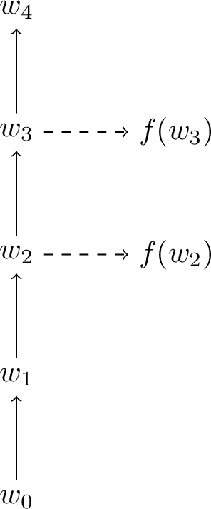
Lemma 3.30. If \(\mathcal{T}\) is a proof search tree for \(\sigma\) with choice rule \(\mathsf{C_f}\) and Prover has a winning strategy in \(\mathcal{G}(\mathcal{T},\mathsf{C_f})\), then \(\sigma\) has a \(\mathrm{nIM}\)-proof.
Proof sketch. As in the proof of Lemma 3.29, the strategy tree of a winning strategy for Prover is a subtree \(\mathcal{S}\) of \(\mathcal{T}\) that contains exactly one child of each node \(u\) labelled by a sequent which is the conclusion of a \(\mathsf{C_f}\)-rule. We obtain a derivation \(\pi\) from \(\mathcal{S}\) as follows. First of all delete all indices from sequents occurring in \(\mathcal{S}\). Then in case the child of \(u\) is not labelled by the premise of the form \(\Gamma_{\tau} \Rightarrow_{(k+1)_m}\Delta_{\tau}\), we can simply view this as an application of \({\rightarrow}\mathsf{R}\) or \(\larger[-1.5]\square\) (possibly with a subsequent application of \(\mathsf{f}\)). In case the direct successor is labelled by the premise of the form \(\Gamma_{\tau} \Rightarrow_{(k+1)_m}\Delta_{\tau}\), we simply view this as no rule application at all, as the left and right side of the sequent have not changed. It is clear that from these steps one can obtain a pre-proof \(\pi\) of \(\sigma\). Due to the winning conditions of Prover, every leaf of \(\mathcal{S}\) must be an axiom and every infinite branch must have a good suffix. Thus \(\pi\) is a \(\mathrm{nIM}\)-proof of \(\sigma\). ◻
Proposition 3.11. If \(\mathcal{T}\) is a proof search tree for \(\sigma\) with choice rule \(\mathsf{C_f}\) and Refuter has a winning strategy in \(\mathcal{G}(\mathcal{T},\mathsf{C_f})\), then \(\sigma\) is falsifiable over the class of functional models.
Proof. Let \(\mathcal{T}\) be a proof search tree for \(\sigma\) and \(e\) be the enumeration of \(\sigma\) where \(\lvert \mathsf{Cl}(\sigma) \rvert = m\). Let \(f\) be a winning strategy for Refuter in \(\mathcal{G}(\mathcal{T},\mathsf{C_f})\) and \(\mathcal{T}_f\) the strategy tree of \(f\). By Lemma 3.28, \(\mathcal{T}_f = \mathcal{R}\) is a refutation. Let \(\mathcal{M}_\mathcal{R}=(W, \leq, R, V)\) be the canonical model based on \(\mathcal{R}\). It is straighforward to check that \(\mathcal{M}_\mathcal{R}\) is a dynamic model. Moreover, since every instance of \(\mathsf{C_f}\) has at most one modal premise, each world in \(\mathcal{M}_\mathcal{R}\) has at most one modal successor, implying that \(\mathcal{M}_\mathcal{R}\) is functional.
We follow the proof of Proposition 3.8. For any formula \(\varphi\), by induction on the structure on \(\varphi\) we simultaneously prove that for any \(w\in W\) we have
\(\mathcal{M},w\models \varphi\) if \(\varphi\in \Gamma^-_{w}\) and
\(\mathcal{M},w\not\models \varphi\) if \(\varphi\in \Delta^-_{w}\),
where \(\Gamma_w \mathrel{\vcenter{:}}= \bigcup_{s \in w} \Gamma_s\) and \(\Delta_w \mathrel{\vcenter{:}}= \bigcup_{s \in w} \Delta_s\). For each \(w \in W\) let \(t_w\) be the unique node in \(w\) which is labelled by the conclusion of a \(\mathsf{C_f}\)-instance. The base cases as well as the cases for \(\varphi = \psi \ast \chi\) with \(\ast \in \{\wedge, \vee, \rightarrow\}\) are identical to the corresponding cases in the proof of Proposition 3.8.
Case for \(\larger[-1.5]\square\). For (a) if \(\larger[-1.5]\square\varphi\in \Gamma^-_w\), then \(\larger[-1.5]\square\varphi \in \Gamma_{t_w}^-\). Suppose \(w\leq v \mathrel{R} u\). Then, by definition of the \(\mathsf{C_f}\)-rule, \(\varphi\in \Gamma^-_{u}\). The induction hypothesis then implies \(\mathcal{M},u\models \varphi\), so \(\mathcal{M},w\models \larger[-1.5]\square\varphi\). For (b) if \(\larger[-1.5]\square\varphi\in \Delta^-_w\), then \(\larger[-1.5]\square\varphi \in \Delta_{t_w}^-\). As \(\Gamma_{t_w}\Rightarrow \Delta_{t_w}\) is the conclusion of a \(\mathsf{C_f}\)-instance, it must be of the form \(\Pi, \larger[-1.5]\square\Gamma \Rightarrow_k \{\varphi_i \rightarrow \psi_i^\mathsf{u}\}_{i=0}^l, \{\larger[-1.5]\square\chi_{j}^{a_j}\}_{j=0}^{r}, \larger[-1.5]\square\varphi^a, \Sigma\) with \(e(\larger[-1.5]\square\varphi^a) = k'\) for some \(k' \leq m\). Now, by construction of \(\leq\) and the rule \(\mathsf{C_f}\), it follows that there exists a \(v\geq w\) such that \(\Gamma_v\Rightarrow \Delta_v\) is equal to \(\Pi, \larger[-1.5]\square\Gamma \Rightarrow_{k'} \{\varphi_i \rightarrow \psi_i^\mathsf{u}\}_{i=0}^l, \{\larger[-1.5]\square\chi_{j}^{a_j}\}_{j=0}^{r}, \larger[-1.5]\square\varphi^a, \Sigma\). So, by construction of \(R\), there exists a \(u\) with \(v\mathrel{R} u\) and \(\varphi \in \Delta^-_{u}\). The induction hypothesis then implies \(\mathcal{M},u\not\models \varphi\), so \(\mathcal{M},w\not\models \larger[-1.5]\square\varphi\).
Case for \(\ooalign{\larger[-1.5]\square\cr \hidewidth\raise.035ex* \mkern 1.12mu\cr}\). For (a) if \(\ooalign{\larger[-1.5]\square\cr \hidewidth\raise.035ex* \mkern 1.12mu\cr}\varphi \in \Gamma_w^-\), then \(\ooalign{\larger[-1.5]\square\cr \hidewidth\raise.035ex* \mkern 1.12mu\cr}\varphi \in \Gamma_{t_w}^-\). Suppose \(w \mathrel{\tilde{R}^*} v\). Let \[w = u_0 \leq u_1 \mathrel R u_2 \leq ... \leq u_{n-1} \mathrel R u_n = v\] be the \(\tilde{R}\)-path from \(w\) to \(v\). We prove inductively that for each \(i \leq n\) holds that \(\varphi, \larger[-1.5]\square\ooalign{\larger[-1.5]\square\cr \hidewidth\raise.035ex* \mkern 1.12mu\cr}\varphi \in \Gamma^-_{u_i}\). For \(u_0 = w\), saturation yields \(\varphi, \larger[-1.5]\square\ooalign{\larger[-1.5]\square\cr \hidewidth\raise.035ex* \mkern 1.12mu\cr}\varphi \in \Gamma_w^-\). For \(i >0\) we have by (the inner) induction hypothesis that \(\varphi, \larger[-1.5]\square\ooalign{\larger[-1.5]\square\cr \hidewidth\raise.035ex* \mkern 1.12mu\cr}\varphi \in \Gamma_{u_{i-1}}^-\). If \(u_{i-1} \mathrel{R}u_i\), then we have \(\ooalign{\larger[-1.5]\square\cr \hidewidth\raise.035ex* \mkern 1.12mu\cr}\varphi \in \Gamma_{u_i}^-\), and so saturation yields \(\varphi, \larger[-1.5]\square\ooalign{\larger[-1.5]\square\cr \hidewidth\raise.035ex* \mkern 1.12mu\cr}\varphi \in \Gamma_{u_i}^-\). Otherwise \(u_{i-1} \leq u_i\). The definition of \(\mathsf{C_f}\) and the fact that invertible rules are applied preservingly implies that \(\varphi, \larger[-1.5]\square\ooalign{\larger[-1.5]\square\cr \hidewidth\raise.035ex* \mkern 1.12mu\cr}\varphi \in \Gamma_{u_i}^-\). Hence \(\varphi \in \Gamma_v^-\), and so by induction hypothesis \(\mathcal{M}, v \models \varphi\). Hence \(\mathcal{M}, w \models \ooalign{\larger[-1.5]\square\cr \hidewidth\raise.035ex* \mkern 1.12mu\cr}\varphi\).
For (b) if \(\ooalign{\larger[-1.5]\square\cr \hidewidth\raise.035ex* \mkern 1.12mu\cr}\varphi \in \Delta_w^-\), then by saturation \(\varphi \in \Delta_{t_w}^-\) or \(\larger[-1.5]\square\ooalign{\larger[-1.5]\square\cr \hidewidth\raise.035ex* \mkern 1.12mu\cr}\varphi \in \Delta_{t_w}^-\). Suppose towards contradiction that for all \(w \mathrel{\tilde{R}^\ast} v\) holds that \(\varphi \not \in \Delta_v^-\). This implies that \(\varphi \not \in \Gamma_{t_w}^-\), hence \(\larger[-1.5]\square\ooalign{\larger[-1.5]\square\cr \hidewidth\raise.035ex* \mkern 1.12mu\cr}\varphi \in \Gamma_{t_w}^-\). Then we can define an infinite path \(\rho\) in \(\mathcal{R}\) starting from \(t_w\) as follows. At each \(\mathsf{C_f}\)-application, pick the modal premise in case \(\ooalign{\larger[-1.5]\square\cr \hidewidth\raise.035ex* \mkern 1.12mu\cr}\varphi^\mathsf{f}\) is the formula in the consequent of its sequent and otherwise pick the right intuitionistic premise. Since \(\larger[-1.5]\square\ooalign{\larger[-1.5]\square\cr \hidewidth\raise.035ex* \mkern 1.12mu\cr}\varphi \in \Delta_{t_w}^-\) and \(e(\larger[-1.5]\square\ooalign{\larger[-1.5]\square\cr \hidewidth\raise.035ex* \mkern 1.12mu\cr}\varphi^a) = k\) for some \(k \leq m\), eventually, when following the path consisting of right intuitionistic premises starting in \(t_w\), the index of the sequent \(\Gamma_{t_w} \Rightarrow \Delta_{t_w}\) will become \(k\), implying that eventually the modal premise of a \(\mathsf{C_f}\)-application will have the formula \(\ooalign{\larger[-1.5]\square\cr \hidewidth\raise.035ex* \mkern 1.12mu\cr}\varphi^\mathsf{f}\) on the right side. On the path from the modal premise of one \(\mathsf{C_f}\)-instance to the conclusion of the next \(\mathsf{C_f}\)-instance, the formula \(\ooalign{\larger[-1.5]\square\cr \hidewidth\raise.035ex* \mkern 1.12mu\cr}\varphi^\mathsf{f}\) must be principal in an instance of \(\ooalign{\larger[-1.5]\square\cr \hidewidth\raise.035ex* \mkern 1.12mu\cr}\mathsf{R}\). Since \(\varphi \not \in \Delta_v^-\) for any \(w \mathrel{\tilde{R}^*} v\), the right premise of this instance is chosen by Refuter, implying that \(\larger[-1.5]\square\ooalign{\larger[-1.5]\square\cr \hidewidth\raise.035ex* \mkern 1.12mu\cr}\varphi^\mathsf{f}\) occurs on the right-hand side of the next saturated sequent and therefore the argument can be iterated. The generated branch \(\rho\) has always a formula in focus (namely \(\ooalign{\larger[-1.5]\square\cr \hidewidth\raise.035ex* \mkern 1.12mu\cr}\varphi\) or \(\larger[-1.5]\square\ooalign{\larger[-1.5]\square\cr \hidewidth\raise.035ex* \mkern 1.12mu\cr}\varphi\)) and passes infinitey often through \(\ooalign{\larger[-1.5]\square\cr \hidewidth\raise.035ex* \mkern 1.12mu\cr}\mathsf{R}\), implying that it has a good suffix. This contradicts the assumption that \(\mathcal{R}\) is a refutation. Thus there exists \(w \mathrel{\tilde{R}^*} v\) with \(\varphi \in \Delta_v^-\). The induction hypothesis implies \(\mathcal{M}, v \not \models \varphi\), hence \(\mathcal{M}, w \not \models \ooalign{\larger[-1.5]\square\cr \hidewidth\raise.035ex* \mkern 1.12mu\cr}\varphi\).
Let \(w \in W\) contain the root of \(\mathcal{R}\). By definition \(\Gamma_\sigma \subseteq \Gamma_w\) and \(\Delta_\sigma \subseteq \Delta_w\). Thus \(\mathcal{M},w \not \models \sigma\). ◻
Combining these results, once again together with determinacy of the game, yields completeness of \(\mathrm{nIM}\) with respect to functional models. The proof of the following theorem is analogous to the proof of Theorem 3.10.
Theorem 3.12 (Completeness of \(\mathrm{nIM}\) with respect to functional models). If a sequent \(\sigma\) is valid over the class of functional models, then \(\sigma\) has a \(\mathrm{nIM}\)-proof.
3.8.4 Translating Non-Wellfounded into Cyclic Proofs↩︎
With completeness of \(\mathrm{nIM}\) for triangle and functional models at hand, we now show that \(\mathrm{cIM}\) is complete by translating non-wellfounded proofs into cyclic proofs. Due to the presence of the focus annotation, the translation is relatively straightforward.
Lemma 3.31. Let \(\rho\) be an infinite branch of an \(\mathrm{nIM}\)-proof \(\pi\). Then \(\rho\) contains a successful repetition.
Proof. Note that each rule of \(\mathrm{nIM}\) (and hence of \(\mathrm{cIM}\)) is analytic in the following sense. If \[\infer[\mathsf{r}]{\sigma}{\sigma_1 & \ldots & \sigma_n}\] is a rule instance of \(\mathsf{r} \in \mathrm{nIM}\), then \(\mathsf{Cl}(\sigma_i) \subseteq \mathsf{Cl}(\sigma)\) for all \(1 \leq i \leq n\). This implies that every sequent occurring in \(\rho\) consists of formulas of \(\mathsf{Cl}(\sigma)\) where \(\sigma\) is the sequent labelling the root of \(\pi\). Since \(\mathsf{Cl}(\sigma)\) is finite by Lemma 3.1, there are only finitely many sequents occurring in \(\rho\). Thus, there exists a sequent \(\Gamma \Rightarrow \Delta\) which labels infinitely many nodes in \(\rho\). Since \(\pi\) is an \(\mathrm{nIM}\)-proof, there exists a good suffix \(\rho'\) of \(\rho\), i.e. every sequent in \(\rho'\) has a formula in focus and \(\rho'\) passes infinitely often through \(\ooalign{\larger[-1.5]\square\cr \hidewidth\raise.035ex* \mkern 1.12mu\cr}\mathsf{R}\) with the principal formula in focus. Let \(i < \omega\) be the least natural number such that \(\rho(i)\) belongs to \(\rho'\) and is labelled by \(\Gamma \Rightarrow \Delta\). Since there are infinitely many nodes labelled by \(\Gamma \Rightarrow \Delta\) in \(\rho'\) and \(\rho'\) passes through infinitely many instances of \(\ooalign{\larger[-1.5]\square\cr \hidewidth\raise.035ex* \mkern 1.12mu\cr}\mathsf{R}\) with the principal formula in focus, there exists a least natural number \(i < j < \omega\) such that \(\rho(j)\) is labelled by \(\Gamma \Rightarrow \Delta\) as well and the path from \(\rho(i)\) to \(\rho(j)\) passes through an instance of \(\ooalign{\larger[-1.5]\square\cr \hidewidth\raise.035ex* \mkern 1.12mu\cr}\mathsf{R}\) with the principal formula in focus. Therefore \((\rho(i), \rho(j))\) is a successful repetition occurring in the branch \(\rho\). ◻
Note that the existence of a successful repetition in \(\rho\) implies the existence of a lowermost successful repetition in \(\rho\).
Definition 3.36. Let \(\pi\) be an \(\mathrm{nIM}\)-proof. The induced cyclic proof* \(\pi_c\) is the subtree of \(\pi\) obtained by pruning every infinite branch at the lowermost successful repetition.*
The following then follows immediately from Lemma 3.31.
Lemma 3.32. If \(\pi\) is an \(\mathrm{nIM}\)-proof, then \(\pi_c\) is a \(\mathrm{cIM}\)-proof.
Proof. Since \(\pi\) is an \(\mathrm{nIM}\)-proof, every infinite branch contains a successful repetition by Lemma 3.31. Therefore, by Kőnig’s Lemma, \(\pi_c\) is finite and every branch \(\rho\) of \(\pi_c\) corresponds to an initial segment of a branch \(\rho'\) of \(\pi\). If \(\rho'\) is a finite branch, then \(\rho = \rho'\) and since \(\pi\) is an \(\mathrm{nIM}\)-proof, \(\rho\) ends in an axiom. Otherwise \(\rho'\) is an infinite branch and \(\rho\) is the initial segment of \(\rho'\) ending at the first successful repetition of \(\rho'\). Thus every leaf of \(\pi_c\) is an axiom or belongs to a successful repetition, implying that \(\pi_c\) is a \(\mathrm{cIM}\)-proof. ◻
Completeness of \(\mathrm{cIM}\) then follows as a corollary of Theorem 3.10, Theorem 3.12 and Lemma 3.32.
Theorem 3.13 (Completeness of \(\mathrm{cIM}\)). If a sequent \(\sigma\) is valid over the classes of dynamic models, of triangle models or of functional models, then \(\sigma\) has a \(\mathrm{cIM}\)-proof.
Proof. By Lemma 3.5 every formula valid over the class of dynamic models is also valid over the classes of functional and of triangle models. Thus suppose \(\sigma\) is valid over the classes of triangle models or functional models. Theorem 3.10 or Theorem 3.12 then imply that \(\sigma\) has an \(\mathrm{nIM}\)-proof \(\pi\). Lemma 3.32 implies that \(\pi_c\) is a \(\mathrm{cIM}\)-proof of \(\sigma\). ◻
Theorem 3.7 and Theorem 3.13 together provide an alternative proof of Theorem 3.1 that \(\mathbf{IM}= \mathbf{IM_t} = \mathbf{IM_f}\).
3.9 Conclusion↩︎
We have introduced a simple intuitionistic dynamic logic called intuitionistic master modality. The following summarizes the results established in this chapter.
We have presented three classes of models to evaluate formulas of \(\mathsf{IM}\), namely dynamic models, triangle models and functional models.
Theorem 3.1 shows that all three classes generate the same set of validities.
We have presented a sound and complete axiomatization for \(\mathsf{IM}\) and established several properties about derivations, such as the Deduction Theorem. The presented completeness proof closely follows the completeness proof for a multi–modal version of \(\mathsf{IM}\) presented by Marti [26] (who uses a different axiomatization) and yields the finite model property for \(\mathsf{IM}\) as well as decidability.
We have developed a sound and complete cyclic calculus for \(\mathsf{IM}\). Completeness was established via a proof search argument, whose robustness was illustrated by giving an alternative proof of Theorem 3.1.
That the language of \(\mathsf{IM}\) without the master modality cannot distinguish between dynamic and triangle models has already been observed by other authors, for example Litak and Visser [65]. Adding the master modality to the language does not impact this result, as in order to evaluate \(\larger[-1.5]\square\) and \(\ooalign{\larger[-1.5]\square\cr \hidewidth\raise.035ex* \mkern 1.12mu\cr}\), the truth conditions of dynamic models consider the same worlds as when one takes the closure under triangle confluence. The result that \(\mathsf{IM}\) cannot distinguish between dynamic and functional models is new and perhaps more surprising. However, this is once again caused by the evaluation of the modalities, where in order to evaluate a \(\larger[-1.5]\square\)-formula at a world \(w\), one has to consider all modal successors of all intuitionistic successors of \(w\). This implies that it does not matter whether we consider models with one or multiple modal successors, as we can always add more intuitionistic successors to obtain additional modal successors. A consequence of Theorem 3.1 is that stronger confluence conditions are needed when we want to obtain an interesting intuitionistic linear temporal logic, namely conditions that allow us to evaluate modalities by only looking at the modal successor of the current world. This will be done in Chapter 5, where we will study dynamic models where the modal accessibility relation is a total function \(f\) which is order-preserving.
Our observations regarding the three classes of models naturally lead to the following question.
Question 3.1. What logic is obtained when evaluating \(\mathcal{L}_\mathrm{IM}\) over functional triangle models?
Over such models \((W, \leq, f, V)\) if \(f\) is a total function, then note that for any world \(w \in W\) and any \(v \geq w\), \(f(w) = f(v)\). In other words, the entire intuitionistic tree rooted at \(w\) has the same modal successor. This implies that the modalities satisfy classical principles like the boxed law of excluded middle: \(\larger[-1.5]\squarep \vee \neg \larger[-1.5]\squarep\) is valid.14 A similar phenomenon will be encountered in Chapter 4 when we combine triangle confluence with frame conditions.
The completeness proof for \(\mathrm{IM_H}\) demonstrates a rather straightforward adaptation of the mathematical methods used to obtain completeness for classical modal logic with the master modality to the intuitionistic case. In fact, the presented canonical model construction combines the canonical model construction for intuitionistic logic (see [46]) with the standard technique to handle the master modality from the classical realm (see e.g. [64]). Due to the lack of strong confluence properties, we can directly define finite canonical models for fragments of the language. As we will see in Chapter 6, this is no longer possible when stronger confluence conditions are considered.
The developed cyclic calculus \(\mathrm{cIM}\) for \(\mathsf{IM}\) is an extension of a multi-succedent calculus for \(\mathsf{IPL}\) with rules for \(\larger[-1.5]\square\) and \(\ooalign{\larger[-1.5]\square\cr \hidewidth\raise.035ex* \mkern 1.12mu\cr}\). Many classical techniques, such as focus annotations and proof search games, are directly applicable to \(\mathsf{IM}\) as demonstrated in this chapter. The main difference between the intuitionistic and the classical case is that the presence of the intuitionistic implication complicates the proof search argument, as we have to deal with falsifying \(\rightarrow\)-formulas in intuitionistic successors and \(\larger[-1.5]\square\)-formulas in modal successors, as opposed to only dealing with the latter in classical modal logic with the master modality (for an in depth study of cyclic proof systems for classical modal logic with the master modality, see the PhD thesis of Rooduijn [63]; for proof search arguments for classical common knowledge logics, see [69]). The increase in the mathematical difficulty is not substantial though, once again due to the lack of strong enough confluence conditions, which allows us to falsify \(\rightarrow\)- and \(\larger[-1.5]\square\)-formulas independently of one another. The system \(\mathrm{cIM}\) is well-behaved: it is analytic and does not require a cut rule; furthermore it also does not require additional structure on sequents such as labels or nesting, and has a simple success condition on cyclic branches. Our work therefore lies the foundation for studying the proof theory of \(\mathsf{IM}\) in more details. In particular, the following questions are left open.
Question 3.1. Does \(\mathsf{IM}\) have Craig/uniform/Lyndon interpolation?
Studer showed that classical common knowledge logics does not have Craig interpolation and hence also not uniform and Lyndon interpolation [70]. The provided counterexample however requires the language to feature at least two agents, which implies that there is hope for obtaining Craig interpolation for \(\mathsf{IM}\). The cyclic system \(\mathrm{cIM}\) is thereby a good starting point for studying this problem from a proof theoretic point of view. Another open proof theoretic question concerns the problem of cut elimination.
Question 3.1. Do \(\mathrm{cIM}\) and \(\mathrm{nIM}\) admit cut elimination?
In recent work, Sierra-Miranda and Studer showed cut elimination for a non-wellfounded proof system for classical modal logic with the master modality [71]. The similarities between their system and \(\mathrm{nIM}\) suggest that their proof may be adaptable to the intuitionistic case.
4 Intuitionistic Common Knowledge Logic↩︎
4.1 Introduction↩︎
Epistemic logic describes a family of logical systems used to reason about knowledge and belief of agents as well as studying various notions of group knowledge. Traditionally, epistemic logics are devised as (classical) modal logics. Given a finite set of agents \(\mathsf{A}\), the language of epistemic logic extends propositional logic with modal operators \(\mathsf{K}_i\) for \(i \in \mathsf{A}\) which are interpreted as the knowledge operator of agent \(i\). Thus a formula of the form \(\mathsf{K}_i \varphi\) is read as ‘agent \(i\) knows that \(\varphi\)’. Of particular interest is the study of nesting of knowledge among different agents, i.e. what agents know about the knowledge of other agents. For example, the formula \(\mathsf{K}_i \mathsf{K}_j \neg \mathsf{K}_i \neg \varphi\) expresses that agent \(i\) knows, that agents \(j\) knows, that agent \(i\) considers \(\varphi\) to be possible. Such kind of reasoning naturally leads to the study of notions of group knowledge. Perhaps the most famous example of such a notion is common knowledge. Informally, among a group of agents a formula \(\varphi\) is common knowledge if every agent knows \(\varphi\) and every agent knows, that every agent knows \(\varphi\), and so on. Write \(\mathsf{E}\varphi\) for ‘everybody (in the group) knows \(\varphi\)’. Formally, \(\mathsf{E}\varphi\) is defined as \[\mathsf{E}\varphi \mathrel{\vcenter{:}}= \bigwedge_{i \in \mathsf{A}} \mathsf{K}_i \varphi.\] As usual, let \(\mathsf{E}^0 \varphi \mathrel{\vcenter{:}}= \varphi\) and \(\mathsf{E}^{n+1} \varphi \mathrel{\vcenter{:}}= \mathsf{E}\mathsf{E}^n \varphi\). Then ‘common knowledge of \(\varphi\)’ is equivalent to the infinite conjunction \[\bigwedge_{k < \omega} E^k \varphi.\] In order to express common knowledge, we use a new operator \(\mathsf{C}\) where \(\mathsf{C}\varphi\) is given as the greatest fixed point of the propositional function \(x \mapsto \varphi \wedge \mathsf{E}x\). Epistemic logic with common knowledge is called common knowledge logic (\(\mathsf{CK}\)) and has found applications in computer science, such as in the study of distributed systems (see e.g. [72]).
Epistemic logic over an intuitionistic base logic, called intuitionistic epistemic logic has been studied at least since the 1990’s and the work by Williamson [38]. In the last decade, several systems of intuitionistic epistemic logic have been developed. These systems fall into two general categories. The first category aims to develop systems of intuitionistic epistemic logic to study knowledge from the point of view of intuitionism. Such systems usually attempt to provide a BHK interpretation of knowledge. In this category falls the work of Williamson [38], the intuitionistic epistemic logic IEL developed by Artemov and Protopopescu [8], as well as recent work about logics of knowing-wh (which are epistemic logics featuring operators to capture different types of knowledge such as knowing-how) and explicit interpretations of intuitionistic logic by Wang et al. (see e.g. [73]–[77]). The second category is primarily motivated by mathematical reasons as well as applications to computer science and studies intuitionistic modal logics, where the \(\larger[-1.5]\square\)-operator is interpreted as a knowledge operator and which are extended by fixed point operators for group knowledge such as common knowledge or distributed knowledge. In particular, logics from this category do not attempt to give a BHK reading of knowledge and largely treat knowledge classically. To this category belongs most notably the intuitionistic common knowledge logic \(\mathsf{ICK}\), developed by Jäger and Marti [25]. Jäger and Marti focus on the mathematical theory of \(\mathsf{ICK}\) by developing a sound and complete axiomatization and a sound and complete sequent calculus with induction rule. Moreover, they also study intuitionistic epistemic logic with distributed knowledge [27], which is further studied in [28], [29]. \(\mathsf{ICK}\) is a multi-modal version of the logic \(\mathsf{IM}\) studied in the previous chapter. Given a finite set of agent names \(\mathsf{A}\), the language features a \(\larger[-1.5]\square\)-operator for each agent \(i \in \mathsf{A}\), written as \(\mathsf{K}_i\). In that setting the master modality becomes more expressive, as it is no longer simply a reflexive transitive closure operator of \(\larger[-1.5]\square\), but instead of \(\mathsf{E}\). For example, it is easily verified that over triangle models where the modal accessibility relation is reflexive and transitive, the master modality is definable in terms of \(\larger[-1.5]\square\). This is not the case in the multi-modal setting of \(\mathsf{ICK}\) with common knowledge. Formulas of \(\mathsf{ICK}\) are evaluated on triangle models, satisfying standard frame conditions such as reflexive triangle models, S4 triangle models and S5 triangle models. Jäger and Marti provide a sequent calculus for \(\mathsf{ICK}\) over the class of triangle and over the class of reflexive triangle models, but do not extend their work to the S4 and S5 case [25]. Furthermore, Marti also provides an axiomatization [69]. The presented sequent calculus characterizes common knowledge via an induction rule, and features a cut rule which is used in the completeness proof. Whether cut elimination is possible is not discussed, however in a similar calculus for classical common knowledge logic presented by Alberucci and Jäger [66], the cut rule cannot be eliminated (at least for the logic over S5 models) and no restriction to analytic cuts is possible, which sheds doubt on whether such an enterprise is possible for \(\mathsf{ICK}\).
In this chapter we aim to use the cyclic calculus developed in Chapter 3 to build a uniform proof theory for \(\mathsf{ICK}\) evaluated over the classes of triangle models, reflexive triangle models, S4 triangle models and S5 triangle models. To that end we will first show how to translate \(\mathrm{cIM}\) into a multi-modal version and then introduce rules for the frame conditions. As it turns out, the adaptation of the calculus to account for reflexive and S4 models is straightforward by adding the standard modal rules for reflexivity and transitivity to the calculus. Moreover, completeness can be established by following the proof search argument introduced in the previous chapter with only minor changes to the ‘choice rule’. The case for S5 is more difficult. First, the combination of triangle confluence with S5 frame conditions results in rather strange models where given a world \(w\), the entire intuitionistic tree rooted at \(w\) belongs to the equivalence class of \(w\) under \(R\). In such a setting knowledge essentially reduces to classical knowledge, which satisfies classical principles such as the ‘boxed law of excluded middle’: for every proposition \(p\), the formula \(\mathsf{K}_i p \vee \neg \mathsf{K}_i p\) is valid. Second, the S5 conditions lead to the standard proof theoretical problems already encountered for classical S5 modal logic: we will show that the extension of \(\mathrm{cIM}\) with rules for the frame conditions is not cut-free complete. This could perhaps be circumvented by passing to labelled or nested sequents, but we will follow the method presented in a joint publication with Rooduijn [41] on classical common knowledge logic over S5 and instead extend the calculus with a cut rule. Analytic completeness is then established via a canonical model construction by restricting applications of the cut rule to analytic cuts. Importantly, the extension with the cut rule allows us to prove completeness directly; a detour to a non-wellfounded system as for \(\mathrm{cIM}\) is no longer required. It is in fact unclear whether the proof search argument can be adapted in the presence of the cut rule. Furthermore, we investigate the relationship between \(\mathsf{ICK}\) over S5 and \(\mathsf{CK}\) over S5 by developing a translation from \(\mathsf{CK}\) into \(\mathsf{ICK}\) and we show that proof search in the cyclic calculus for the S5 case can be automated by reducing the problem of finding proofs to the problem of solving a certain parity game. Finally, combining the translation and parity game, we show that the problem of finding proofs in the cyclic calculus for \(\mathsf{ICK}\) over S5 triangle models is ExpTime-complete.
4.2 Syntax and Semantics↩︎
Let \(\mathsf{A}\) be a finite set of agent names. The language \(\mathcal{L}_\mathsf{ICK}\) extends \(\mathcal{L}_\mathsf{IPL}\) by modal operators \(\mathsf{K}_i\) for \(i \in \mathsf{A}\) and the fixed point operator \(\mathsf{C}\), where \(\mathsf{C}\varphi\) is characterized as the greatest fixed point of the propositional function \(x \mapsto \varphi \wedge \mathsf{E}x\). Formulas of \(\mathcal{L}_\mathrm{ICK}\) are defined by the following grammar in Backus-Naur form: \[\varphi ::= \bot \, \lvert \, p \, \lvert \, \varphi \wedge \varphi \, \lvert \, \varphi \vee \varphi \, \lvert \, \varphi \rightarrow \varphi \, \lvert \, \mathsf{K}_i \varphi \, \lvert \, \mathsf{C}\varphi.\] where \(p \in \mathsf{Prop}\) and \(i \in \mathsf{A}\). The modal operator \(K_i\) is the knowledge operator of agent \(i\): \(\mathsf{K}_i \varphi\) is read as ‘agent i knows \(\varphi\)’. The modal operator \(\mathsf{C}\) is the common knowledge operator: \(\mathsf{C}\varphi\) is read as ‘\(\varphi\) is common knowledge (among the agents in \(\mathsf{A}\))’. The modality \(\mathsf{E}\), read as ‘everybody knows’, is defined by \[\mathsf{E}\varphi \mathrel{\vcenter{:}}= \bigwedge_{i \in \mathsf{A}} K_i \varphi.\] Due to the presence of multiple knowledge operators, the definition of the closure of a formula (c.f. Definition 3.1) is adjusted as follows.
Definition 4.1. The closure* \(\mathsf{Cl}(\varphi)\) of a formula \(\varphi\) is defined by induction on \(\varphi\) as follows.*
\(\mathsf{Cl}(\bot) = \{\bot\}\)
\(\mathsf{Cl}(p) = \{ p \}\) for \(p \in \mathsf{Prop}\)
\(\mathsf{Cl}(\varphi \ast \psi) = \mathsf{Cl}(\varphi) \cup \mathsf{Cl}(\psi) \cup \{ \varphi \ast \psi\}\) for \(\ast \in \{\wedge, \vee, \rightarrow\}\)
\(\mathsf{Cl}(\mathsf{K}_i \varphi) = \mathsf{Cl}(\varphi) \cup \{\mathsf{K}_i \varphi\}\)
\(\mathsf{Cl}(\mathsf{C}\varphi) = \mathsf{Cl}(\varphi) \cup \{\mathsf{C}\varphi\} \cup \{ \mathsf{K}_i \mathsf{C}\varphi \mid i \in \mathsf{A}\}\)
Given a set \(\Gamma\) of formulas, the closure* \(\mathsf{Cl}(\Gamma)\) of \(\Gamma\) is defined by \[\mathsf{Cl}(\Gamma):= \bigcup_{\varphi\in\Gamma}\mathsf{Cl}(\varphi).\] A set of formulas \(\Gamma\) is closed if \(\Gamma = \mathsf{Cl}(\Gamma)\).*
Additionally, we define the negation closure of a formula, which will be used to treat \(\mathsf{ICK}\) over S5 models.
Definition 4.2. The negation closure* \(\mathsf{Cl}^\neg(\varphi)\) of a formula \(\varphi\) is the least closed set of formulas containing \(\varphi\), such that whenever \(\mathsf{K}_i \psi \in \mathsf{Cl}^\neg(\varphi)\), then \(\neg \mathsf{K}_i \psi \in \mathsf{Cl}^\neg(\varphi)\). The negation closure \(\mathsf{Cl}^\neg(\Gamma)\) of a set of formulas \(\Gamma\) is given by \[\mathsf{Cl}^\neg(\Gamma) \mathrel{\vcenter{:}}= \bigcup_{\varphi \in \Gamma} \mathsf{Cl}^\neg (\varphi).\] A set \(\Gamma\) is negation closed if \(\Gamma = \mathsf{Cl}^\neg(\Gamma)\).*
The following lemma is easily verified by an induction on the structure of formulas.
Lemma 4.1. For any formula \(\varphi\), \(\mathsf{Cl}(\varphi)\) and \(\mathsf{Cl}^\neg(\varphi)\) are finite. Moreover, if \(\Gamma\) is a finite set of formulas, then \(\mathsf{Cl}(\Gamma)\) and \(\mathsf{Cl}^\neg(\Gamma)\) are finite.
The complexity of a formula is defined as follows.
Definition 4.3. The complexity* \(c(\varphi)\) of a formula \(\varphi\) is defined inductively as follows.*
\(c(\bot) = c(p) = 0\)
\(c(\varphi \ast \psi) = c(\varphi) + c(\psi) +1\) for \(\ast \in \{\wedge, \vee, \rightarrow\}\)
\(c(\mathsf{K}_i \varphi) = c(\mathsf{C}\varphi) = c(\varphi) + 1\)
Given a finite set of formulas \(\Gamma\), the complexity* of \(\Gamma\) is defined as \[c(\Gamma) = \sum_{\varphi \in \Gamma}c(\varphi).\]*
Formulas of \(\mathcal{L}_\mathrm{ICK}\) are evaluated over triangle models equipped with a modal accessibility relations for each agent. We follow [25] and call such models (intuitionistic) epistemic models.
Definition 4.4. An (intuitionistic) epistemic model* is a tuple \(\mathcal{M}=(W, \leq, \{R_i\}_{i \in \mathsf{A}}, V)\) such that \((W, \leq, R_i, V)\) is a triangle model for each \(i \in \mathsf{A}\).*
Given an epistemic model \(\mathcal{M}=(W, \leq, \{R_i\}_{i \in \mathsf{A}}, V)\), define the relation \[R := \bigcup_{i \in A} R_i\] and let \(R^*\) be the reflexive and transitive closure of \(R\).
Definition 4.5. The truth relation* \(\models_t\) between worlds \(w\) of an epistemic model \(\mathcal{M}\) and formulas \(\varphi\) extends Definition 2.7 by the following clauses.*
| \(M,w \models_t \mathsf{K}_i \varphi\) | iff | for all \(v \in W\) if \(w \mathrel{R_i} v\), then \(M,v \models \varphi\) |
| \(M, w \models_t \mathsf{C}\varphi\) | iff | for all \(v \in W\) if \(w \mathrel{R^*} v\), then \(M,v \models \varphi\) |
Since only triangle models are studied in this chapter, we will supress the index \(t\) in \(\models_t\) and simply write \(\models\). The notions of satisfiability and validity are defined as before. Since \(\mathsf{ICK}\) is simply a multi-modal version of \(\mathsf{IM}\) it is obvious that the monotonicity lemma (c.f. Lemma 3.2) still holds.
We will study \(\mathcal{L}_\mathsf{ICK}\) over the classes of epistemic models, reflexive epistemic models, S4 epistemic models and S5 epistemic models. The definition of these classes of models is a generalization of Definition 2.20.
Definition 4.6. An epistemic model \(\mathcal{M}=(W, \leq, \{R_i\}_{i \in \mathsf{A}}, V)\) is called a
**reflexive epistemic model* if for each \(i \in \mathsf{A}\), \(R_i\) is reflexive;*
**S4 epistemic model* if for each \(i \in \mathsf{A}\), \(R_i\) is reflexive and transitive;*
**S5 epistemic model* if for each \(i \in \mathsf{A}\), \(R_i\) is reflexive, transitive and symmetric.*
For simplicity we will usually refer to reflexive epistemic models simply as reflexive models throughout this chapter, and similarly for S4 and S5 epistemic models.
Definition 4.7. Denote by \(\mathbf{ICK}\) the set of valid formulas over the class of epistemic models. Furthermore, denote by \(\mathbf{ICK_\ast}\) for \(\mathbf{\ast} \in \{\mathbf{T}, \mathbf{S4}, \mathbf{S5}\}\) the set of valid formulas over the classes of reflexive, S4 and S5 models, respectively.
Note that \(\mathbf{ICK} \subseteq \mathbf{ICK_T} \subseteq \mathbf{ICK_{S4}} \subseteq \mathbf{ICK_{S5}}\). The following lemma shows that the logics \(\mathbf{ICK}\), \(\mathbf{ICK_T}\) and \(\mathbf{ICK_{S4}}\) contain the standard validities of classical epistemic logic regarding the knowledge and common knowledge operators (see e.g. [64] for axiomatizations of classical common knowledge logics over different frame conditions). The proof is by standard semantical arguments using the frame conditions that the models of the relevant logic satisfy and is omitted.
Lemma 4.2. Let \(\varphi, \psi\) be formulas and \(i \in \mathsf{A}\). Then
\(\mathsf{K}_i (\varphi \rightarrow \psi) \rightarrow (\mathsf{K}_i \varphi \rightarrow \mathsf{K}_i \psi) \in \mathbf{ICK}\);
\(\mathsf{C}(\varphi \rightarrow \psi) \rightarrow (\mathsf{C}\varphi \rightarrow \mathsf{C}\psi) \in \mathbf{ICK}\);
\(\mathsf{K}_i \varphi \rightarrow \varphi \in \mathbf{ICK_T}\);
\(\mathsf{K}_i \varphi \rightarrow \mathsf{K}_i \mathsf{K}_i \varphi \in \mathbf{ICK_{S4}}\).
The logic \(\mathbf{ICK_{S5}}\), on the other hand, contains some validities that are rather unexpected in the context of intuitionistic logic. The combination of S5 frame conditions with triangle confluence has a strong impact on the models and thus on the resulting logic. Given worlds \(w\) and \(v\) if \(w \leq v\), then by reflexivity \(v \mathrel{R_i} v\) and so by triangle confluence \(w \mathrel{R_i} v\) for all \(i \in \mathsf{A}\). In other words, the intuitionistic order is a subset of each modal accessibility relation: \({\leq} \subseteq {R_i}\) for each \(i \in \mathsf{A}\) (note that this already holds for S4 models). Moreover, by symmetry, we obtain that \(v \mathrel{R_i} w\), implying that given \(w\), the entire intuitionistic tree rooted at \(w\) belongs to the equivalence class of \(w\) under the equivalence relation induced by \(R_i\).
This leads to an interesting observation. Since every intuitionistic successor \(v\) of \(w\) belongs to the equivalence class of \(w\), every world accessible from \(v\) is accessible from \(w\) and vice versa, implying that for \(w \leq v\), \(w \models \mathsf{K}_i \varphi\) if and only \(v \models \mathsf{K}_i \varphi\). Moreover, since truth is persistent in \(\leq\) and falsity is persistent in \(\geq\), implications with a ‘boxed’ antecedent (i.e. formulas of the form \(\mathsf{K}_i \varphi \rightarrow \psi\) or \(\mathsf{C}\varphi \rightarrow \psi\)) are evaluated classically, as shown in the following lemma.
Lemma 4.3. Let \(\mathcal{M}\) be an S5 model, \(w\) a world, \(i \in \mathsf{A}\) and \(\varphi, \psi \in \mathcal{L}_\mathsf{ICK}\). Then the following holds.
\(\mathcal{M}, w \models \mathsf{K}_i \varphi \rightarrow \psi\) if and only if \(\mathcal{M}, w \not \models \mathsf{K}_i \varphi\) or \(\mathcal{M}, w \models \psi\).
Proof. For the left–to–right direction suppose \(\mathcal{M}, w \models \mathsf{K}_i \varphi \rightarrow \psi\). Then for all \(w \leq v\) if \(\mathcal{M}, v \models \mathsf{K}_i \varphi\), then \(\mathcal{M}, v \models \psi\). Thus, for \(v=w\), \(\mathcal{M}, w \not \models \mathsf{K}_i \varphi\) or \(\mathcal{M}, w \models \psi\). For the right–to–left direction we proceed by contraposition. Suppose \(\mathcal{M}, w \not \models \mathsf{K}_i \varphi \rightarrow \psi\). Then there exists \(w \leq v\) such that \(\mathcal{M}, v \models \mathsf{K}_i \varphi\) and \(\mathcal{M}, v \not \models \psi\). Since \(w \leq v\), by the Monotonicity Lemma \(\mathcal{M}, w \not \models \psi\). Now suppose \(w \mathrel{R}_i u\). Since \(w \leq v\) and \(v \mathrel{R}_i v\) by reflexivity of \(R_i\), triangle confluence implies that \(w \mathrel{R}_i v\). By symmetry of \(R_i\) we \(v \mathrel{R}_i w\) and so by transitivity of \(R_i\), \(v \mathrel{R}_i u\). Thus \(\mathcal{M}, u \models \varphi\), implying that \(\mathcal{M}, w \models \mathsf{K}_i \varphi\). ◻
As a corollary we obtain that \(\mathsf{ICK}\) over S5 models satisfies a boxed version of the law of excluded middle: for any formula \(\varphi\) the formula \(\mathsf{K}_i \varphi \vee \neg \mathsf{K}_i \varphi\) is valid. The proof is omitted.
Corollary 4.1. Let \(\varphi\) be a formula and \(i \in \mathsf{A}\). Then
\(\mathsf{K}_i \varphi \vee \neg \mathsf{K}_i \varphi \in \mathbf{ICK_{S5}}\);
\(\mathsf{C}\varphi \vee \neg \mathsf{C}\varphi \in \mathbf{ICK_{S5}}\);
\(\neg \mathsf{K}_i \varphi \rightarrow \mathsf{K}_i \neg \mathsf{K}_i \varphi \in \mathbf{ICK_{S5}}\).
4.3 Cyclic Calculi↩︎
This section introduces four sequent calculi for \(\mathsf{ICK}\) with the aim to capture the validities of \(\mathsf{ICK}\) over the classes of all epistemic models, reflexive models, S4 models and S5 models. Each calculus shares the same set of basic rules as \(\mathrm{cIM}\) and additional rules for the modalities, which differ depending on which frame condition ought to be captured. The calculus for \(\mathsf{ICK}\) over the class of epistemic models is denoted \(\mathrm{cICK}\) and is simply a multi-modal version of \(\mathrm{cIM}\). The calculi \(\mathrm{cICK}_{\mathrm{T}}\), \(\mathrm{cICK}_{\mathrm{S4}}\) and \(\mathrm{cICK}_{\mathrm{S5}}\) are modular extensions of \(\mathrm{cICK}\). The focus lies mostly on \(\mathrm{cICK}_{\mathrm{S5}}\), which is the extension of \(\mathrm{cICK}\) by two rules for the modalities and, additionally, the cut rule and a special rule dealing with implications \(\varphi \rightarrow \psi\) where \(\varphi\) is a boxed formula. We begin by introducing the basic components of the calculi. Since \(\mathrm{cICK}\) and its extensions are multi-modal versions of \(\mathrm{cIM}\), most definitions are identical or similar to the case of \(\mathsf{IM}\); for convenience we briefly repeat the basic definitions here and refer the reader to Chapter 3, Section 3.6 for further details.
An annotated formula is a tuple \((\varphi, a)\), written \(\varphi^a\), where \(\varphi \in \mathcal{L}_\mathsf{ICK}\) and \(a \in \{\mathsf{u}, \mathsf{f}\}\). The annotation \(\mathsf{u}\) designates that the formula is unfocused and \(\mathsf{f}\) that the formula is in focus.
Definition 4.8. A sequent* is an ordered pair of finite sets of annotated formulas \(\Gamma \Rightarrow \Delta\) such that*
Every formula in \(\Gamma\) is unfocused.
At most one formula in \(\Delta\) is in focus.
If a formula \(\varphi\) is in focus, then \(\varphi = \mathsf{C}\psi\) or \(\varphi = \mathsf{K}_i \mathsf{C}\psi\) for some formula \(\psi\) and \(i \in \mathsf{A}\).
We denote sequents by \(\sigma\) and write \(\Gamma_\sigma\) and \(\Delta_\sigma\) for the left and right side of \(\sigma\), respectively. The interpretaion of a sequent \(\sigma\) is the formula \(\sigma^I \mathrel{\vcenter{:}}= \bigwedge \Gamma_\sigma^- \rightarrow \bigvee \Delta_\sigma^-\). The closure \(\mathsf{Cl}(\sigma)\) of a sequent \(\sigma\) is defined as \(\mathsf{Cl}(\sigma) \mathrel{\vcenter{:}}= \mathsf{Cl}(\Gamma_\sigma) \cup \mathsf{Cl}(\Delta_\sigma)\). Additionally, the negation closure of a sequent \(\sigma\) is defined as \(\mathsf{Cl}^\neg (\sigma) \mathrel{\vcenter{:}}= \mathsf{Cl}^\neg(\Gamma_\sigma) \cup \mathsf{Cl}^\neg (\Delta_\sigma)\). Each calculus consists of all of the basic rules depicted in Table 5 and additionally some of the rules depicted in Table 6.
Definition 4.9. Consider the rules depicted in Table 5 and Table 6.
The calculus \(\mathrm{cICK}\) consists of the basic rules from Table 5 as well as the rules \(\mathsf{K_i}\) for \(i \in \mathsf{A}\), \(\mathsf{C}\mathsf{L}\) and \(\mathsf{C}\mathsf{R}\).
The calculus \(\mathrm{cICK}_\mathrm{T}\) is the extension of \(\mathrm{cICK}\) with the rules \(\mathsf{T_i}\) for \(i \in \mathsf{A}\).
The calculus \(\mathrm{cICK}_\mathrm{S4}\) is the calculus \(\mathrm{cICK}_\mathrm{T}\) with the rules \(\mathsf{K_i}\) replaced by the rules \(\mathsf{S4_i}\) for \(i \in \mathsf{A}\).
The calculus \(\mathrm{cICK}_\mathrm{S5}\) is the calculus \(\mathrm{cICK}_\mathrm{S4}\) with the rules \(\mathsf{S4_i}\) replaced by the rules \(\mathsf{S5_i}\) and extended by the rules \(\mathsf{K_i} {\rightarrow}\) and \(\mathsf{cut}\) for \(i \in \mathsf{A}\).
| \(\infer[\mathsf{id}]{\Gamma, \varphi^\u \Rightarrow \varphi^a, \Delta}{}\) | \(\infer[\bot]{\Gamma, \bot^\u \Rightarrow \Delta}{}\) |
| \(\infer[\wedge \mathsf{L}]{\Gamma, \varphi \wedge \psi^\u \Rightarrow \Delta}{\Gamma, \varphi^\u, \psi^\u \Rightarrow \Delta}\) | \(\infer[\wedge \mathsf{R}]{\Gamma\Rightarrow \varphi \wedge \psi^\u ,\Delta}{\Gamma \Rightarrow \varphi^\u, \Delta & \Gamma \Rightarrow \psi^\u, \Delta}\) |
| \(\infer[\vee \mathsf{L}]{\Gamma, \varphi \vee \psi^\u\Rightarrow \Delta}{\Gamma, \varphi^\u \Rightarrow \Delta & \Gamma, \psi^\u \Rightarrow \Delta}\) | \(\infer[\vee \mathsf{R}]{\Gamma \Rightarrow \varphi \vee \psi^\u, \Delta}{\Gamma \Rightarrow \varphi^\u, \psi^\u, \Delta}\) |
| \(\infer[{\to} \mathsf{L}]{\Gamma, \varphi \rightarrow \psi^\u\Rightarrow \Delta}{\Gamma, \varphi \rightarrow \psi^\u \Rightarrow \varphi^\u, \Delta & \Gamma, \psi^\u \Rightarrow \Delta}\) | \(\infer[{\to} \mathsf{R}]{\Gamma \Rightarrow \varphi \rightarrow \psi^\u, \Delta}{\Gamma, \varphi^\u \Rightarrow \psi^\u}\) |
| \(\infer[\mathsf{u}]{\Gamma \Rightarrow \varphi^\f, \Delta}{\Gamma \Rightarrow \varphi^\u, \Delta}\) | \(\infer[\mathsf{f}]{\Gamma \Rightarrow \varphi^\u, \Delta}{\Gamma \Rightarrow \varphi^\f, \Delta}\) |
| \(\infer[\mathsf{K_i}]{\Pi, \K_i \Gamma \Rightarrow \K_i \varphi^a, \Sigma}{\Gamma \Rightarrow \varphi^a}\) | \(\infer[\mathsf{cut}]{\Gamma \Rightarrow \Delta}{\Gamma, \varphi^\u \Rightarrow \Delta & \Gamma \Rightarrow \varphi^\u, \Delta}\) |
| \(\infer[\mathsf{T_i}]{\Gamma, \K_i \varphi^\u \Rightarrow \Delta}{\Gamma, \varphi^\u \Rightarrow \Delta}\) | \(\infer[\mathsf{S4_i}]{\Pi, \K_i \Gamma \Rightarrow \K_i \varphi^a, \Sigma}{ \K_i \Gamma \Rightarrow \varphi^a}\) |
| \(\infer[\mathsf{S5_i}]{\Pi, \K_i \Gamma \Rightarrow \K_i \varphi^a, \K_i \Delta, \Sigma}{ \K_i \Gamma \Rightarrow \varphi^a, \K_i \Delta}\) | \(\infer[\mathsf{K_i}{\rightarrow}]{\Gamma \Rightarrow \K_i \varphi \rightarrow \psi^\u, \Delta}{\Gamma, \K_i \varphi^\u \Rightarrow \psi^\u, \Delta}\) |
| \(\infer[\C \mathsf{L}]{\Gamma, \C \varphi^\u \Rightarrow \Delta}{\Gamma, \varphi^\u, \{\K_i \C \varphi^\u\}_{i \in \A} \Rightarrow \Delta}\) | \(\infer[\C \mathsf{R}]{\Gamma \Rightarrow \C \varphi^a,\Delta}{\Gamma \Rightarrow \varphi^\u, \Delta & \{\Gamma \Rightarrow \K_i \C \varphi^a, \Delta\}_{i \in \A}}\) |
For every rule in Table 5 as well the rules \(\mathsf{CL}\), \(\mathsf{CR}\) and \(\mathsf{K_i}{\rightarrow}\), the distinguished formula in the conclusion is called principal and the distinguished formulas in the premises are its residuals. For example, in the rule \(\mathsf{\mathsf{C}L}\) the principal formula is \(\mathsf{C}\varphi^\mathsf{u}\) and the residual formulas are \(\varphi^\mathsf{u}\) and \(\mathsf{K}_i \mathsf{C}\varphi^\mathsf{u}\) for \(i \in \mathsf{A}\). The rule \(\mathsf{cut}\) has no principal formulas, while both distinguished formulas in the premises are residual. These distinguished formulas are called the cut formulas. For the knowledge rules for agent \(i\) (i.e. \(\mathsf{K_i}\), \(\mathsf{T_i}\), \(\mathsf{S4_i}\) and \(\mathsf{S5_i}\)) every formula in the conclusion is principal and every formula in the premise is the residual of the corresponding principal formula. Formulas in \(\Sigma, \Pi\) have no residual formulas. All other formulas occurring in a rule are called side formulas.
4.3.1 Cyclic Proofs↩︎
We define the notion of cyclic proof for each system introduced above. Once again, the definitions simply adapt the definitions for \(\mathsf{IM}\) to the case for \(\mathsf{ICK}\).
Let \(\mathsf{P} \in \{\mathrm{cICK}, \mathrm{cICK}_\mathrm{T}, \mathrm{cICK}_\mathrm{S4}, \mathrm{cICK}_\mathrm{S5}\}\). A \(\mathsf{P}\)-pre-proof of a sequent \(\sigma\) is a finite tree \(\pi\) labeled by sequents according to the rules of \(\mathsf{P}\) and whose root is labeled by \(\sigma\).
Definition 4.10. A path \(\rho\) through a pre-proof \(\pi\) is successful* if the following hold.*
Every sequent in \(\rho\) has a formula in focus.
The path \(\rho\) passes through an instance of the rule \(\mathsf{C}\mathsf{R}\) where the principal formula is in focus.
Given a pre-proof \(\pi\), a pair of nodes \((u,v)\) of \(\pi\) is a repetition if \(u \not = v\), there exists a path from \(u\) to \(v\) and both nodes are labeled by the same sequent. A repetition \((u,v)\) is successful if the path from \(u\) to \(v\) is successful.
Definition 4.11. A cyclic proof* of a sequent \(\sigma\) in \(\mathsf{P}\) is a \(\mathsf{P}\)-pre-proof \(\pi\) of \(\sigma\) such that every leaf \(v\) of \(\pi\) is labeled by an axiom or there exists a node \(u\) in \(\pi\) such that \((u,v)\) form a successful repetition. If a sequent \(\sigma\) has a proof in \(\mathsf{P}\), then we say that \(\sigma\) is \(\mathsf{P}\)-provable.*
An example of a cyclic proof showing that \(\mathsf{C}\varphi^\mathsf{u}\Rightarrow \mathsf{C}(\varphi \vee \psi)^\mathsf{u}\) is \(\mathrm{cICK}\)-provable is displayed in Figure 9, where it is assumed that \(\mathsf{A}=\{1,2\}\). By inspecting the proof it is obvious that the example can be generalized to \(n\) agents for any natural number \(n>0\). Note that the presented calculi combine standard rules for \(\mathsf{IPL}\) and for common knowledge logic (see for example [41], [47]). The only exception is the calculus \(\mathrm{cICK}_{\mathrm{S5}}\) which features the rule \({\rightarrow}\mathsf{K_i}\). This rule formalizes the observation from Lemma 4.3 that implications of the form \(\mathsf{K}_i \varphi \rightarrow \psi\) behave classically. Observe that the rule is only applicable if the principal formula is of the form \(\mathsf{K}_i \varphi \rightarrow \psi\). It is therefore a special case of the classical right implication rule. We now give two examples showing that \(\mathrm{cICK}_{\mathrm{S5}}\) proves the boxed law of excluded middle for \(\mathsf{K}_i\) and \(\mathsf{C}\), which illustrate how the rule \({\rightarrow}\mathsf{K_i}\) can be used to prove classical principles.
Example 4.1. The sequent \(\Rightarrow \mathsf{K}_i p \vee \neg \mathsf{K}_i p^\mathsf{u}\) is provable in \(\mathrm{cICK}_\mathsf{S5}\). Recall that \(\neg \varphi\) is a shortcut for \(\varphi \rightarrow \bot\).
Note that with the standard intuitionistic right implication rule, this proof is not possible: if \({\rightarrow}\mathsf{R}\) is applied (bottom-up) to the sequent \(\Rightarrow \mathsf{K}_i p^\mathsf{u}, \mathsf{K}_i p \rightarrow \bot^\mathsf{u}\), the premise is \(\mathsf{K}_i p^\mathsf{u}\Rightarrow \bot^\mathsf{u}\), which is not provable.
Example 4.2. The following is a proof of \(\Rightarrow \mathsf{C}p \vee \neg \mathsf{C}p^\mathsf{u}\). For simplicity we assume that there is only one agent in the language, whose knowledge operator is \(\mathsf{K}_i\). The proof is generalized in a straightforward way for multiple agents. Let \(\pi\) be the following proof:
Let \(\tau\) be the following proof:
Finally, the following is then a cyclic proof of \(\Rightarrow \mathsf{C}p \vee \neg \mathsf{C}p^\mathsf{u}\):

Example 4.2 hints towards the fact that \(\mathrm{cICK}_\mathsf{S5}\) is not cut-free complete. This does not come as a surprise, given that it is well-known that classical S5 modal logic does not have a cut-free (plain) sequent calculus. A famous counterexample in the classical realm is the formula \(p \rightarrow \Box \Diamond p\). In the intuitionistic setting, \(\Box\) and \(\Diamond\) are not interdefinable, therefore our language cannot express \(\Diamond\). However, we may still use the formula as a counterexample, by identifying \(\Box\) with \(\mathsf{K}_i\) and \(\Diamond\) with \(\neg \mathsf{K}_i \neg\). An easy computation shows that \(\neg \mathsf{K}_i \neg\) is not evaluated as a \(\Diamond\), but instead its truth conditions are as follows: \(\mathcal{M}, w \models \neg \mathsf{K}_i \neg \varphi\) if and only if there exist \(u,u' \in W\) with \(w \mathrel{R_i} u\), \(u \leq u'\) and \(\mathcal{M}, u' \models \varphi\). Therefore the following holds.
Lemma 4.4. The formula \(p \rightarrow \mathsf{K}_i \neg \mathsf{K}_i \neg p\) is valid over the class of S5 models.
Proof. Let \(\mathcal{M}=(W, \leq, \{R_i\}_{i \in \mathsf{A}}, V)\) be an arbitrary S5 model and \(w \in W\) an arbitrary world. Let \(v \geq w\) and suppose that \(\mathcal{M},v \models p\). Let \(u \in W\) be any world such that \(v \mathrel{R_i} u\). We want to show that \(\mathcal{M}, u \models \neg \mathsf{K}_i \neg p\). By the previous observation it suffices to find worlds \(s,t\) such that \(u \mathrel{R_i} s\), \(s \leq t\) and \(\mathcal{M},t \models p\). By symmetry \(u \mathrel{R_i} v\). Since \(v \leq v\) and \(\mathcal{M},v \models p\), choosing \(s = t = v\) shows that \(\mathcal{M}, u \models \neg \mathsf{K}_i p\) and hence that \(\mathcal{M},v \models \mathsf{K}_i \neg \mathsf{K}_i \neg p\). Hence \(\mathcal{M},w \models p \rightarrow \mathsf{K}_i \neg \mathsf{K}_i \neg p\), implying that \(p \rightarrow \mathsf{K}_i \neg \mathsf{K}_i \neg p\) is valid. ◻
Proposition 4.1. \(\mathrm{cICK}_\mathsf{S5}\) is not cut-free complete.
Proof sketch. Observe that the sequent \(\sigma = (p^\mathsf{u}\Rightarrow \mathsf{K}_i \neg \mathsf{K}_i \neg p^\mathsf{u})\) does not contain a formula with a common knowledge operator. Therefore, the focus rules cannot be applied, implying that any proof of \(\sigma\) must be a proof where every branch ends in an axiom. Applying rules bottom-up, by inspection of the rules, the only rule applicable to \(\sigma\) (apart from \(\mathsf{cut}\)) is \(\mathsf{S5_i}\). There are two possible such applications. The first application has the sequent \(\Rightarrow \neg \mathsf{K}_i \neg p^\mathsf{u}\) as premise and the second has the sequent \(\Rightarrow \neg \mathsf{K}_i \neg p^\mathsf{u}, \mathsf{K}_i \neg \mathsf{K}_i \neg p^\mathsf{u}\) as premise (this case happens if \(\mathsf{K}_i \neg \mathsf{K}_i \neg p^\mathsf{u}\) in the conclusion is assumed to be contained in \(\mathsf{K}_i \Delta\); see the definition of the rule \(\mathsf{S5_i}\)). It is routine to check that both sequents cannot be proven.15 ◻
Note that the cut formulas used in the cyclic proof in Example 4.2 belong to the negation closure of the root sequent. Similarly, the sequent \(p^\mathsf{u}\Rightarrow K_i \neg K_i \neg p^\mathsf{u}\) is provable by using \(\neg K_i \neg p^\mathsf{u}\) as cut formula, which also belongs to the negation closure of the root sequent. Following this observation we will show that \(\mathrm{cICK}_\mathsf{S5}\) is complete when the cut-rule is restricted to analytic cuts, i.e. instances of \(\mathsf{cut}\) where the cut formula belongs to the negation closure of the root sequent. Therefore we will still obtain analytic completeness for \(\mathrm{cICK}_\mathsf{S5}\).
4.4 Soundness↩︎
This section establishes the soundness of all cyclic systems introduced before. We follow the same strategy as for the soundness proof of \(\mathrm{cIM}\) in Section 3.7, but some small adaptions are needed. The following lemma is routine (c.f. Lemma 3.13).
Lemma 4.5. All rules \(\mathsf{r}\) depicted in Table 5 and Table 6 preserve validity (over the respective class of models): if the conclusion of \(\mathsf{r}\) is invalid, the one of the premises is invalid.
Let \(\sigma\) be a sequent with a formula in focus, i.e. \(\Delta_\sigma\) contains a formula of the form \(\mathsf{K}_i^j \mathsf{C}\varphi^\mathsf{f}\) for \(j \in \{0,1\}\). Denote by \(\sigma(n)\) the sequent \(\Gamma_\sigma \Rightarrow \Delta_\sigma, \mathsf{K}_i^j \mathsf{E}^n \varphi^\mathsf{u}\), i.e. the sequent expanding the right side of \(\sigma\) by the formula \(\mathsf{K}_i^j \mathsf{E}^n \varphi^\mathsf{u}\). The following lemma is then proven as Lemma 3.24.
Lemma 4.6. If \(\sigma\) has a formula in focus and is invalid (over one of the classes of epistemic, reflexive, S4 or S5 models), then there exists a natural number \(n\) such that \(\sigma(n)\) is invalid.
Therefore we may define the following measure,
\[\mu(\sigma) := \min \{n < \omega \, \mid \, \sigma(n) \text{ is invalid}\}\]
and then prove a strengthening of Lemma 4.5.
Lemma 4.7. Suppose \[\infer[\mathsf{r}]{\sigma}{\sigma_1 & \dotsm & \sigma_n}\] is an instance of a rule in Table 5 or Table 6. If \(\sigma\) is invalid (over the respective class of models), then there is a natural number \(1 \leq k \leq n\) such that \(\sigma_k\) is invalid. If both \(\sigma\) and \(\sigma_k\) have a formula in focus, then, moreover, \[\mu(\sigma_k) \leq \mu(\sigma),\] where the inequality is strict if \(\mathsf{r} = \mathsf{C}\mathsf{R}\) and the principal formula is in focus.
Proof. The proof is similar to the proof of Lemma 3.25. We only treat the new cases in which the formula in focus is principal. This implies that \(\mathsf{r} \in \{\mathsf{K_i}, \mathsf{S4_i}, \mathsf{S5_i}, \mathsf{CR}\}\). The case for \(\mathsf{K_i}\) is similar to the case for \(\larger[-1.5]\square\) in the proof of Lemma 3.25 and we omit it.
Case for \(\mathsf{r} = \mathsf{S5_i}\). In this case the conclusion \(\sigma\) is of the form: \[\Pi, \mathsf{K}_i \Gamma \Rightarrow \mathsf{K}_i \mathsf{C}\psi^\mathsf{f}, \mathsf{K}_i \Delta, \Sigma.\] Since \(\sigma\) is invalid, there is a pointed S5 model \((\mathcal{M}, w)\) such that \(\mathcal{M}, w \not \models \sigma(n)\) where \(n= \mu(\sigma)\). Thus there exists \(w' \geq w\) such that \(\mathcal{M}, w' \models \bigwedge \Gamma_\sigma^-\) and \(\mathcal{M}, w' \not \models \bigvee \Delta_\sigma^- \vee \mathsf{K}_i \mathsf{E}^n \psi\). In particular it holds that \[\mathcal{M}, w' \not \models \mathsf{K}_i \mathsf{E}^{n} \psi.\] It follows that there is a world \(v \in W\) such that \(w' \mathrel{R_i} v\) and \(\mathcal{M}, v \not \models \mathsf{E}^n \psi\). Clearly this also means that \(\mathcal{M}, v \not \models \mathsf{C}\psi\). We claim that, in fact, \[\mathcal{M},v \not \models (\mathsf{K}_i \Gamma \Rightarrow \mathsf{C}\psi^\mathsf{f}, \mathsf{E}^n \psi^\mathsf{u}, \mathsf{K}_i\Delta)^I,\] which implies that the premise \(\sigma_1\) is invalid and that \(\mu(\sigma_1) \leq \mu(\sigma)\).
By the fact that \(R_i\) is transitive, it holds for all \(\varphi\) with \(\mathcal{M}, w' \models \mathsf{K}_i \varphi\) that \(\mathcal{M}, v \models \mathsf{K}_i \varphi\). Hence \(M, v \models \mathsf{K}_i \varphi\) for each \(\mathsf{K}_i \varphi^\mathsf{u}\in \mathsf{K}_i \Gamma\). Moreover, suppose that \(\mathsf{K}_i \psi^a \in \mathsf{K}_i \Delta\). Then \(\mathcal{M}, w' \not \models \mathsf{K}_i \psi\). Thus there is a state \(u \in W\) such that \(w' \mathrel{R_i} u\) and \(\mathcal{M}, u \not \models \psi\). By symmetry and transitivity, we get \(v \mathrel{R_i} u\), whence \(\mathcal{M}, v \not \models \mathsf{K}_i \psi\), as required.
Case for \(\mathsf{r} = \mathsf{S4_i}\). For this case observe that \(\mathsf{S4_i}\) is a special case of \(\mathsf{S5_i}\), namely it consists of all instances of \(\mathsf{S5_i}\) where \(\mathsf{K}_i \Delta = \emptyset\). In the case above, the symmetry of \(R_i\) is exclusively used to deal with formulas in \(\mathsf{K}_i \Delta\). Hence, we obtain the result by following the previous case using a pointed S4 model instead of a pointed S5 model, and skipping the part dealing with \(\mathsf{K}_i \Delta\).
Case for \(\mathsf{r} = \mathsf{CR}\). In this case the conclusion \(\sigma\) is of the form \(\Gamma \Rightarrow \mathsf{C}\varphi^\mathsf{f}, \Delta\) with premises \(\sigma_0\) given by \(\Gamma \Rightarrow \varphi^\mathsf{u}, \Delta\), and \(\sigma_i\) for \(1 \leq i \leq n\) given by \(\Gamma \Rightarrow \mathsf{K}_i\mathsf{C}\varphi^\mathsf{f}, \Delta\), respectively. As there exists a pointed epistemic model \((\mathcal{M},w)\) that falsifies \(\sigma(\mu(\sigma))\), \(w\) has an intuitionistic successor \(v\) such that \(\mathcal{M},v\models \bigwedge \Gamma^-\) and \(\mathcal{M},v\not\models \mathsf{C}\varphi \lor \mathsf{E}^{\mu(\sigma)} \varphi\lor \bigvee\Delta^{-}\). If \(\mu(\sigma) = 0\), then \(\mathcal{M},v \not \models \varphi\), so \((\mathcal{M},v)\) falsifies the left premise \(\sigma_0\). By Lemma 3.21, \(\sigma_0\) does not have a formula in focus, and so the statement of the lemma holds. If \(\mu(\sigma) > 0\), then \(\mathcal{M},v \not \models \mathsf{K}_i\mathsf{E}^{\mu(\sigma) - 1} \varphi\) for some \(i \in \mathsf{A}\). Hence \((\mathcal{M},v)\) falsifies \(\sigma_i(\mu(\sigma)-1)\). So \(\sigma_i\) is invalid and we have \(\mu(\sigma_i) < \mu(\sigma)\). ◻
Soundness for each cyclic calculus then follows by the same argument as used to prove Theorem 3.7.
Theorem 4.2 (Soundness of \(\mathrm{cICK}_\ast\)). Let \(\sigma\) be a sequent. The following hold.
If \(\sigma\) is \(\mathrm{cICK}\)-provable, then \(\sigma\) is valid over the class of epistemic models.
If \(\sigma\) is \(\mathrm{cICK}_\mathrm{T}\)-provable, then \(\sigma\) is valid over the class of reflexive epistemic models.
If \(\sigma\) is \(\mathrm{cICK}_\mathrm{S4}\)-provable, then \(\sigma\) is valid over the class of S4 epistemic models.
If \(\sigma\) is \(\mathrm{cICK}_\mathrm{S5}\)-provable, then \(\sigma\) is valid over the class of S5 epistemic models.
4.5 Completeness↩︎
This section establishes completeness of all cyclic calculi introduced above. Completeness of \(\mathrm{cICK}, \mathrm{cICK}_\mathrm{T}\) and \(\mathrm{cICK}_\mathrm{S4}\) for their respective classes of models will be shown by using the proof search technique introduced in Section 3.5. Since the resulting proofs are very similar, only brief sketches are provided. The main part of this section is the completeness proof for \(\mathrm{cICK}_\mathsf{S5}\).
4.5.1 Completeness for Epistemic, Reflexive and S4 Models↩︎
In order to prove completeness of \(\mathrm{cICK}\), \(\mathrm{cICK}_\mathsf{T}\) and \(\mathrm{cICK}_\mathsf{S4}\), we define corresponding non-wellfounded calculi \(\mathsf{nICK}\), \(\mathsf{nICK_T}\) and \(\mathsf{nICK_{S4}}\) following the definitions in Section 3.6. We then employ the same proof search strategy, where the definition of a saturated sequent is adapted from the definition for \(\mathrm{nIM}\) in the obvious way. Proof search trees are defined in Definition 3.27 (by replacing \(\ooalign{\larger[-1.5]\square\cr \hidewidth\raise.035ex* \mkern 1.12mu\cr}\) with \(\mathsf{C}\)). Neither the indexes nor the enumeration of the formulas in \(\mathsf{Cl}(\sigma)\) are needed and so are ignored henceforth. Proof search games are defined as for \(\mathrm{nIM}\). The definition of the canonical model has to be adapted to the multi-modal case: given a choice rule \(\mathsf{C}\), we assume that the modal premises are partitioned into \(\lvert \mathsf{A}\rvert\) groups. Then replace clause 3. in Definition 3.33 by the following clause.
For each \(i \in \mathsf{A}\), \(R_i \subseteq W \times W\) is such that
\(w \mathrel{R_i} v\) iff there exists \(s \in w\) and \(t \in v\) such that \(s\) is the conclusion and \(t\) a modal premise from group \(i\) of the same \(\mathsf{C}\)-rule instance.
The calculus \(\mathsf{nICK}\) is simply a multi-modal version of \(\mathrm{nIM}\), so for the choice rule a slightly adapted version of \(\mathsf{C_t}\) suffices to obtain completeness, namely the rule \[\infer[\mathsf{C_t'}]{\Pi, \{\mathsf{K}_i \Gamma_i\}_{i \in \mathsf{A}} \Rightarrow \{(\varphi_i \rightarrow \psi_i)^{\mathsf{u}}\}_{i=0}^l,\{\{\mathsf{K}_i\chi^{a_{i_j}}_{i_j}\}_{j=0}^{m_i}\}_{i \in \mathsf{A}}, \Sigma}{\Pi, \{\mathsf{K}_i \Gamma_i\}_{i \in \mathsf{A}}, \varphi^\mathsf{u}_0 \Rightarrow \psi^{\mathsf{u}}_0 &\dotsm & \Pi, \{\mathsf{K}_i \Gamma_i\}_{i \in \mathsf{A}}, \varphi^\mathsf{u}_l \Rightarrow \psi^{\mathsf{u}}_l & \{ \{\Gamma_i \Rightarrow \chi^{b_{i_j}}_{i_j}\}_{j = 0}^{m_i}\}_{i \in \mathsf{A}}}\] where the annotations \(b_{i_j}\) are equal to \(\mathsf{f}\) whenever the underlying formula \(\chi_{i_j}\) is a \(\mathsf{C}\)-formula, and equal to \(\mathsf{u}\) otherwise. Moreover, we require that \(\Pi\cup\Sigma\) contains no \(\mathsf{K}_i\)-formulas for any \(i \in \mathsf{A}\) and that \(\Sigma\) contains no \(\rightarrow\)-formulas. The modal premises are those of the form \(\Gamma_i \Rightarrow \chi^{b_{i_j}}_{i_j}\), where \(\{\Gamma_i \Rightarrow \chi_{i_j}^{b_{i_j}}\}_{j = 0}^{m_i}\) is group \(i\) and the others are the intuitionistic premises. In case the conclusion of a \(\mathsf{C_t}'\)-instance has no \(\rightarrow\)- or \(\mathsf{K}_i\)-formulas on the right-hand side for \(i \in \mathsf{A}\), then we stipulate that \(l = -1\) or \(m_i=-1\), respectively.
Observe that the conclusion and each modal premise form an instance of the rule \(\mathsf{K_i}\). It is then routine to show that winning strategies for Prover correspond to \(\mathrm{cICK}\)-proofs and winning strategies for Refuter to refutations. Finally, when proving that refutions induce countermodels, as in the proof of Proposition 3.8, we take the canonical model induced by the refutation, close it under triangle confluence16 and then show that it falsifies the root sequent of the refutation. The proof is similar to the proof of Proposition 3.8.
For \(\mathsf{nICK_T}\) the definition of saturated sequent has to be extended with the following clause:
- If \(\mathsf{K}_i \varphi^\mathsf{u}\in \Gamma\), then \(\varphi^\mathsf{u}\in \Gamma\).
Note that the rule \(\mathsf{T_i}\) is invertible. Hence the same choice rule \(\mathsf{C_t}'\) can be used and when proving that refutations induce a countermodel, we only have to close the modal relations of the canonical model under reflexivity. The additional saturation clause 8. ensures that for any world \(w\) of the canonical model \(\mathcal{M}\) and any formula \(\mathsf{K}_i \varphi\) holds that if \(\mathcal{M}, w \models \mathsf{K}_i \varphi\), then \(\mathcal{M}, w \models \varphi\).
Finally, for \(\mathsf{nICK_{S4}}\) we employ the following choice rule \[\infer[\mathsf{C_{S4}}]{\Pi, \{\mathsf{K}_i \Gamma_i\}_{i \in \mathsf{A}} \Rightarrow \{(\varphi_i \rightarrow \psi_i)^{\mathsf{u}}\}_{i=0}^l,\{\{\mathsf{K}_i\chi^{a_{i_j}}_{i_j}\}_{j=0}^{m_i}\}_{i \in \mathsf{A}}, \Sigma}{\Pi, \{\mathsf{K}_i \Gamma_i\}_{i \in \mathsf{A}}, \varphi^\mathsf{u}_0 \Rightarrow \psi^{\mathsf{u}}_0 &\dotsm & \Pi, \{\mathsf{K}_i \Gamma_i\}_{i \in \mathsf{A}}, \varphi^\mathsf{u}_l \Rightarrow \psi^{\mathsf{u}}_l & \{ \{\mathsf{K}_i \Gamma_i \Rightarrow \chi^{b_{i_j}}_{i_j}\}_{j = 0}^{m_i}\}_{i \in \mathsf{A}}}\] with the same conditions as for \(\mathsf{C_t}'\). Note that the only difference to \(\mathsf{C_t}'\) is that the applications of \(\mathsf{K_i}\) were replaced by applications of \(\mathsf{S4_i}\). When proving that refutations induce countermodels, it then suffices to close the modal accessibility relations of the canonical model induced by the refutation under reflexivity and transitivity. Note that since formulas in \(\mathsf{K}_i \Gamma\) are preserved when moving to a modal premise of group \(i\), closing the modal accessibility relation \(R_i\) under transitivity does not lead to the failure of any formula in \(\mathsf{K}_i \Gamma\). Therefore we obtain completeness for the non-wellfounded calculi \(\mathsf{nICK}\), \(\mathsf{nICK_T}\) and \(\mathsf{nICK_{S4}}\). By following the construction given in Lemma 3.32 we obtain completeness for the cyclic calculi.
Theorem 4.3 (Completeness of \(\mathrm{cICK}\), \(\mathrm{cICK}_{\mathsf{T}}\) and \(\mathrm{cICK}_\mathsf{S4}\)). Let \(\sigma\) be a sequent. The following hold.
If \(\sigma\) is valid over the class of epistemic models, then \(\sigma\) is \(\mathrm{cICK}\)-provable.
If \(\sigma\) is valid over the class of reflexive epistemic models, then \(\sigma\) is \(\mathrm{cICK}_{\mathsf{T}}\)-provable.
If \(\sigma\) is valid over the class of S4 epistemic models, then \(\sigma\) is \(\mathrm{cICK}_\mathsf{S4}\)-provable.
4.5.2 Completeness for S5 Models↩︎
This section shows that \(\mathrm{cICK}_\mathsf{S5}\) is complete with respect to the class of S5 epistemic models. Due to the presence of \(\mathsf{cut}\) we can prove completeness directly via a canonical model construction, which arguably simplifies the completeness proof. To obtain analytic completeness, applications of \(\mathsf{cut}\) will be restricted to a finite set of formulas relevant to the root sequent. So far we counted as relevant the formulas in the closure of the root sequent. However, as we have seen, the logic \(\mathbf{ICK_{S5}}\) satisfies many classical principles, implying that we need a stronger notion of closure to obtain completeness, namely the negation closure. In the following we provide the basic definitions and lemmas to obtain the canonical model for \(\mathrm{cICK}_\mathsf{S5}\).
Definition 4.12. Let \(\Sigma\) be a non-empty, negation closed and finite set of formulas. A sequent \(\sigma\) is called a
**\(\Sigma\)-sequent* if \(\Gamma_\sigma \cup \Delta_\sigma \subseteq \Sigma\);*
**\(\Sigma\)-provable* if there exists a \(\mathrm{cICK}_\mathsf{S5}\)-proof of \(\sigma\) in which only \(\Sigma\)-sequents occur;*
**\(\Sigma\)-saturated* if \(\sigma\) is \(\Sigma\)-unprovable and \(\Gamma_\sigma \cup \Delta_\sigma = \Sigma\).*
\(\Sigma\)-saturated sequents will be the worlds of the canonical model. Let us first prove an analogue of the Lindenbaum Lemma for saturated sequents.
Lemma 4.8 (Lindenbaum). If a \(\Sigma\)-sequent \(\sigma\) is \(\Sigma\)-unprovable, then there exists a \(\Sigma\)-saturated sequent \(\sigma'\) with \(\Gamma_\sigma \subseteq \Gamma_\sigma'\) and \(\Delta_\sigma \subseteq \Delta_\sigma'\).
Proof. Suppose \(\sigma\) is \(\Sigma\)-unprovable. Let \(\pi\) be the pre-proof of \(\sigma\) built as follows: starting with \(\sigma\) at the root, repeatedly apply the rule \(\mathsf{cut}\) bottom-up to introduce fresh \(\Sigma\)-formulas (i.e. formulas not yet occurring in the conclusion) until every leaf is labelled by a sequent \(\Gamma \Rightarrow \Delta\) with \(\Gamma \cup \Delta = \Sigma\). At least one of these sequents must be \(\Sigma\)-unprovable (and thus \(\Sigma\)-saturated), as otherwise \(\pi\) could be extended into a \(\Sigma\)-proof of \(\sigma\). Note that the saturated sequent extends \(\sigma\). ◻
Next, we will establish some important properties of saturated sequents, that will become useful in the proof of the Truth Lemma (c.f. Lemma 4.11).
Lemma 4.9. Let \(\Gamma \Rightarrow \Delta\) be a \(\Sigma\)-saturated sequent.
If \(\varphi \wedge \psi \in \Sigma\), then \(\varphi \wedge \psi \in \Gamma^-\) if and only if \(\varphi \in \Gamma^-\) and \(\psi \in \Gamma^-\).
If \(\varphi \vee \psi \in \Sigma\), then \(\varphi \vee \psi \in \Gamma^-\) if and only if \(\varphi \in \Gamma^-\) or \(\psi \in \Gamma^-\).
If \(\mathsf{K}_i \varphi \in \Gamma^-\), then \(\varphi \in \Gamma^-\) for all \(i \in \mathsf{A}\).
\(\mathsf{K}_i \varphi \in \Gamma^-\) if and only if \(\neg \mathsf{K}_i \varphi \in \Delta^-\) for all \(i \in \mathsf{A}\).
\(\mathsf{C}\varphi \in \Gamma^-\) if and only if \(\varphi \in \Gamma^-\) and \(\mathsf{K}_i \mathsf{C}\varphi \in \Gamma^-\) for all \(i \in \mathsf{A}\).
Proof. 1. Let \(\varphi \wedge \psi \in \Sigma\) and suppose towards contradiction that \(\varphi \wedge \psi \in \Gamma^-\) but (without loss of
generality) \(\varphi \not \in \Gamma^-\). By saturation \(\varphi \in \Delta^-\). Thus \(\Gamma \Rightarrow \Delta\) is \(\Sigma\)-provable by applying \(\wedge\mathsf{L}\) with principal formula \(\varphi \wedge \psi\) and then the axiom \(\mathsf{id}\).
For the other direction suppose that \(\varphi \wedge \psi \in \Sigma\) and both \(\varphi \in \Gamma^-\) and \(\psi \in \Gamma^-\). Assume towards
contradiction that \(\varphi \wedge \psi \not \in \Gamma^-\). By saturation \(\varphi \wedge \psi \in \Delta^-\). Thus \(\Gamma \Rightarrow \Delta\) is \(\Sigma\)-provable by applying \(\wedge \mathsf{R}\) with principal formula \(\varphi \wedge \psi\) and then the axiom \(\mathsf{id}\) in both resulting branches. The proofs of 2. and 3. are analogous by using the rules for disjunction and the rule \(\mathsf{T_i}\), respectively.
4. Suppose towards contradiction that \(\mathsf{K}_i \varphi \in \Gamma^-\) and \(\neg \mathsf{K}_i \varphi \not \in \Delta^-\). Note that \(\mathsf{K}_i \varphi \in \Gamma\) implies \(\mathsf{K}_i \varphi \in \Sigma\) and since \(\Sigma\) is negation closed, \(\neg
\mathsf{K}_i \varphi \in \Sigma\) as well. By saturation \(\neg \mathsf{K}_i \varphi \in \Gamma^-\). Then \(\Gamma \Rightarrow \Delta\) is \(\Sigma\)-provable by applying \({\rightarrow}\mathsf{L}\) with principal formula \(\mathsf{K}_i \varphi \rightarrow \bot^\mathsf{u}\) and then the axiom \(\mathsf{id}\) in the left branch and the axiom \(\bot\) in the right branch. For the other direction suppose towards contradiction that \(\neg \mathsf{K}_i \varphi \in
\Delta^-\) and \(\mathsf{K}_i \varphi \not \in \Gamma^-\). By saturation \(\mathsf{K}_i \varphi \in \Delta^-\). Then \(\Gamma \Rightarrow \Delta\) is
\(\Sigma\)-provable by applying \({\rightarrow}\mathsf{K_i}\) and then \(\mathsf{id}\). The proof of 5. is standard and omitted. ◻
Given a set of formulas \(\Gamma\), let \(\mathsf{K}_i^{-1} \Gamma \mathrel{\vcenter{:}}= \{\varphi \mid \mathsf{K}_i \varphi \in \Gamma\}\). The canonical model relative to \(\Sigma\) is defined as follows.
Definition 4.13. Let \(\Sigma\) be a non-empty, negation closed and finite set of formulas. The canonical model* (relative to \(\Sigma)\) is given by \(\mathcal{M}^\Sigma =(W^\Sigma, \leq^\Sigma, \{R_i^\Sigma\}_{i \in \mathsf{A}}, V^\Sigma)\) where*
\(W^\Sigma := \{\Gamma^- \mid \Gamma \Rightarrow \Delta \text{ is a \Sigma-saturated sequent}\}\);
\(A \leq^\Sigma B\) if and only if \(A \subseteq B\);
\(A \mathrel{R}_i^\Sigma B\) if and only if \(\mathsf{K}_i \mathsf{K}_i^{-1} A = \mathsf{K}_i \mathsf{K}_i^{-1} B\);
\(V^\Sigma(A) := A \cap \mathsf{Prop}\);
where \(A, B \in W^\Sigma\).
Lemma 4.10. The canonical model is an S5 epistemic model.
Proof. That \((W^\Sigma, \leq^\Sigma)\) is a partial order and each \(R_i^\Sigma\) is reflexive, transitive and symmetric is immediate. Furthermore, by definition of \(V^\Sigma\) and \(\leq^\Sigma\) the valuation is monotone. It remains to show that each \(R_i^\Sigma\) is triangle confluent. Suppose that \(A \leq^\Sigma B\) and \(B \mathrel{R_i^\Sigma} C\). By definition \(\mathsf{K}_i \mathsf{K}_i^{-1} B = \mathsf{K}_i \mathsf{K}_i^{-1}C\). Moreover, \(\mathsf{K}_i \mathsf{K}_i^{-1} A \subseteq \mathsf{K}_i \mathsf{K}_i^{-1} B\). Suppose towards contradiction that there exists a formula \(\mathsf{K}_i \varphi \in B\) such that \(\mathsf{K}_i \varphi \not \in A\). Let \(A = \Gamma^-\) where \(\Gamma \Rightarrow \Delta\) is a saturated sequent. By saturation \(\mathsf{K}_i \varphi \in \Delta^-\). By Lemma 4.9, \(\neg \mathsf{K}_i \varphi \in \Gamma^-\). Hence \(\neg \mathsf{K}_i \varphi \in B\), contradicting that \(\mathsf{K}_i \varphi \in B\). Therefore \(\mathsf{K}_i \mathsf{K}_i^{-1} A = \mathsf{K}_i \mathsf{K}_i^{-1} B = \mathsf{K}_i \mathsf{K}_i^{-1} C\), implying that \(A \mathrel{R_i^\Sigma} C\). ◻
Lemma 4.11 (Truth Lemma). Let \(\Sigma\) be a non-empty, negation closed and finite set of formulas and \(\mathcal{M}^\Sigma =(W^\Sigma, \leq^\Sigma, \{R_i^\Sigma\}_{i \in \mathsf{A}}, V^\Sigma)\) the canonical model relative to \(\Sigma\). Then for any \(\varphi \in \Sigma\) and any \(A \in W^\Sigma\) the following holds.
\(\varphi \in A\) if and only if \(\mathcal{M}^\Sigma, A \models \varphi\).
Proof. By induction on the structure of \(\varphi\). For \(\varphi = \bot\) observe that if \(\bot \in A\) and \(A = \Gamma^-\) where \(\Gamma \Rightarrow \Delta\) is \(\Sigma\)-saturated, then \(\Gamma \Rightarrow \Delta\) is \(\Sigma\)-provable by applying \(\bot\). Hence \(\bot \not \in A\) and by definition \(\mathcal{M}^\Sigma, A \not \models \bot\). For \(\varphi = p\) where \(p \in \mathsf{Prop}\), observe that \(p \in A\) if and only if \(p \in V^\Sigma(A)\) if and only if \(\mathcal{M}^\Sigma, A \models p\). The cases for \(\varphi = \psi \wedge \chi\) and \(\varphi = \psi \vee \chi\) follow directly from Lemma 4.9 and the induction hypothesis.
Case for \(\varphi = \psi \rightarrow \chi\). First suppose that \(\psi \rightarrow \chi \in A\). We want to show that \({\mathcal{M}^\Sigma, A \models \psi \rightarrow \chi}\). Let \(B \in W^\Sigma\) be any world such that \(A \leq^\Sigma B\). Hence \(A \subseteq B\) and so \(\psi \rightarrow \chi \in B\). Suppose \(\mathcal{M}^\Sigma, B \models \psi\). By induction hypothesis \(\psi \in B\). Let \(\Gamma \Rightarrow \Delta\) be \(\Sigma\)-saturated such that \(B = \Gamma^-\). Suppose towards contradiction that \(\chi \in \Delta^-\). We may assume without loss of generality that \(\chi\) occurs unfocused in \(\Delta\). Write \(\Gamma_0\) for \(\Gamma \setminus \{\psi^\mathsf{u}, \psi \rightarrow \chi^\mathsf{u}\}\) and \(\Delta_0\) for \(\Delta \setminus \{\chi^\mathsf{u}\}\). The following is a \(\Sigma\)-proof of \(\Gamma \Rightarrow \Delta\), which contradicts the assumption that \(\Gamma \Rightarrow \Delta\) is \(\Sigma\)-saturated:
Thus \(\chi \in B\) and the induction hypothesis yields \(\mathcal{M}^\Sigma, B \models \psi\). Hence \(\mathcal{M}^\Sigma, A \models \psi \rightarrow \chi\).
For the other direction suppose \(\psi \rightarrow \chi \not \in A\). Let \(A = \Gamma^-\) and let \(\Gamma \Rightarrow \Delta\) be \(\Sigma\)-saturated. By assumption \(\psi \rightarrow \chi \in \Delta^-\). Apply the rule \({\rightarrow}\mathsf{R}\) to \(\psi \rightarrow \chi\). The premise of this application is \(\Gamma, \psi^\mathsf{u}\Rightarrow \chi^\mathsf{u}\) which must be \(\Sigma\)-unprovable. Lemma 4.8 implies that there exists a \(\Sigma\)-saturated sequent \(\Gamma' \Rightarrow \Delta'\) with \(\Gamma, \psi^\mathsf{u}\subseteq \Gamma'\). Let \(B = \Gamma'^-\). By construction \(A \leq^\Sigma B\) and \(\psi \in B\) and \(\chi \not \in B\). Hence by induction hypothesis \(\mathcal{M}^\Sigma, B \models \psi\) and \(\mathcal{M}^\Sigma, B \not \models \chi\). Thus \(\mathcal{M}^\Sigma, A \not \models \psi \rightarrow \chi\).
Case for \(\varphi = \mathsf{K}_i \psi\). First suppose that \(\mathsf{K}_i \psi \in A\). Let \(B \in W^\Sigma\) be any world such that \(A \mathrel{R^\Sigma_i} B\). By definition \(\mathsf{K}_i \psi \in B\) and so by Lemma 4.9, \(\psi \in B\). Hence, by induction hypothesis, \(\mathcal{M}^\Sigma, B \models \psi\), implying that \(\mathcal{M}^\Sigma, A \models \mathsf{K}_i \psi\).
For the other direction suppose \(\mathsf{K}_i \psi \not \in A\). Let \(\Gamma \Rightarrow \Delta\) be \(\Sigma\)-saturated such that \(A = \Gamma^-\). By saturation \(\mathsf{K}_i\psi^a \in \Delta\) for some \(a \in \{\mathsf{u}, \mathsf{f}\}\). Let \(\Delta_0 = \Delta \setminus \{\mathsf{K}_i \psi^a \}\). Observe that the sequent \[\mathsf{K}_i \mathsf{K}_i^{-1} \Gamma \Rightarrow \psi^a, \mathsf{K}_i \mathsf{K}_i^{-1} \Delta_0\] is \(\Sigma\)-unprovable, as otherwise, by an application of \(\mathsf{S5_i}\) we could derive \(\Gamma \Rightarrow \Delta\). By Lemma 4.8 there exists a saturated sequent \(\Gamma' \Rightarrow \Delta'\) such that \(\mathsf{K}_i\mathsf{K}_i^{-1}\Gamma \subseteq \Gamma'\) and, moreover, \({\{\psi^a \} \cup \mathsf{K}_i \mathsf{K}^{-1} \Delta_0 \subseteq \Delta'}\). Let \(B = \Gamma'^-\). By construction \(\psi \not \in \Gamma'^-\) and so the induction hypothesis yields \(\mathcal{M}^\Sigma, B \not \models \psi\). It remains to show that \(A \mathrel{R_i^\Sigma} B\). By construction \(\mathsf{K}_i \mathsf{K}_i^{-1} A \subseteq \mathsf{K}_i \mathsf{K}_i^{-1} B\). For the other direction first observe that \(\mathsf{K}_i \psi \not \in B\), as otherwise \(\psi \in B\). Suppose \(\mathsf{K}_i \gamma \in B\). Then \(\mathsf{K}_i \gamma \not \in \Delta'^-\), and hence in particular \(\mathsf{K}_i \gamma \not \in \Delta^-\). Thus, by saturation, \(\mathsf{K}_i \gamma \in A\). Therefore \(A \mathrel{R_i^\Sigma} B\) and so \(\mathcal{M}^\Sigma, A \not \models \mathsf{K}_i \psi\).
Case for \(\varphi = \mathsf{C}\psi\). First suppose that \(\mathsf{C}\psi \in A\). We want to show that \(\mathcal{M}^\Sigma, B \models \psi\) for any \(B \in W^\Sigma\) such that \(A \mathrel{(R^\Sigma)^*} B\). We prove by induction on the length \(n\) of the path from \(A\) to \(B\) that \(\psi \in B\) and \(\mathsf{C}\psi \in B\). For the base case by assumption \(\mathsf{C}\psi \in A\). Moreover, by Lemma 4.9, \(\psi \in A\). For the induction step suppose that \(A \mathrel{(R^\Sigma)^n} B_0\) and \(B_0 \mathrel{R_i^\Sigma} B\) for some \(i \in \mathsf{A}\). By (the inner) induction hypothesis \(\psi \in B_0\) and \(\mathsf{C}\psi \in B_0\). By Lemma 4.9 also \(\mathsf{K}_i \mathsf{C}\psi \in B_0\). Hence, by definition of \(R_i^\Sigma\), we have that \(\mathsf{K}_i \mathsf{C}\psi \in B\). Lemma 4.9 implies that \(\mathsf{C}\psi \in B\) and \(\psi \in B\). Hence \(\psi \in B\) for any \(A \mathrel{(R^\Sigma)^*} B\). By (the outer) induction hypothesis \(\mathcal{M}^\Sigma, B \models \psi\) for any \(A \mathrel{(R^\Sigma)^*} B\) and therefore \(\mathcal{M}^\Sigma, A \models \mathsf{C}\psi\).
In case \(\mathsf{C}\psi \notin A\), consider a \(\Sigma\)-saturated sequent \(\Gamma \Rightarrow \Delta\) such that \(A = \Gamma^-\). By the presence of the rules \(\mathsf{u}\) and \(\mathsf{f}\), we may assume without loss of generality that \(\mathsf{C}\psi^\mathsf{f}\in \Delta\). Now suppose, towards a contradiction, that \(\mathcal{M}^\Sigma, A \models \mathsf{C}\psi\). For every \(A \mathrel{(R^\Sigma)^*} B\) then holds that \(\mathcal{M}^\Sigma, B \models \psi\). In particular, it follows that \(\mathcal{M}^\Sigma, A \models \psi\), whence, by the induction hypothesis, we have \(\psi^\mathsf{u}\in \Gamma\).
Let \(\Delta_0 = \Delta \setminus \{\mathsf{C}\psi^\mathsf{f}\}\). Consider the following proof, where we assume without loss of generality that there are \(n\) agents:
where each \(\pi_i\) is constructed as follows:
In the above proof the sequent \(\sigma'\) is given by \[\sigma' = \mathsf{K}_i \mathsf{K}_i^{-1} \Gamma \Rightarrow \psi^\mathsf{u}, \mathsf{K}_i \mathsf{K}_i^{-1} \Delta_0\] and the proof \(\pi'\) is obtained from the \(\Sigma\)-provability of \(\sigma'\). Indeed, if \(\sigma'\) were not \(\Sigma\)-provable, then by applying Lemma 4.8 and the induction hypothesis, we would obtain a saturated sequent \(\Gamma' \Rightarrow \Delta'\) extending \(\sigma'\) and a world \(B = \Gamma'^-\) such that \(\mathcal{M}^\Sigma, B \not \models \psi\). First note that \(\mathsf{K}_i \mathsf{C}\psi \not \in B\), as otherwise \(\psi \in B\), implying that the sequent \(\Gamma' \Rightarrow \Delta'\) is an instance of \(\mathsf{id}\) and hence \(\Sigma\)-provable. Therefore \(\mathsf{K}_i \mathsf{C}\psi \in \Delta'^-\). Note that \(A \mathrel{R_i^\Sigma} B\): by construction \(\mathsf{K}_i \mathsf{K}_i^{-1} A \subseteq \mathsf{K}_i \mathsf{K}_i^{-1} B\). Suppose towards contradiction that there exists a formula \(\mathsf{K}_i \chi \in B\) such that \(\mathsf{K}_i \chi \not \in A\). Hence \(\mathsf{K}_i \chi \not \in \Gamma^-\) and so by saturation \(\mathsf{K}_i \chi \in \Delta^-\). Since \(\chi \not = \mathsf{C}\psi\), \(\mathsf{K}_i \chi \in \Delta_0\) and so \(\mathsf{K}_i \chi \in \mathsf{K}_i \mathsf{K}_i^{-1} \Delta_0^-\). Therefore \(\mathsf{K}_i \chi \in \Delta'^-\), implying that \(\mathsf{K}_i \chi \not \in B\), a contradiction. Therefore \(A \mathrel{R_i^\Sigma} B\). Since \(\mathcal{M}^\Sigma, B \not \models \psi\), this contradicts the assumption that \(\mathcal{M}^\Sigma, A \models \mathsf{C}\psi\). Hence, \(\sigma'\) must be \(\Sigma\)-provable.
Furthermore, each sequent \(\sigma'_l\) for \(1 \leq l \leq n\) in the derivation \(\pi_i\) is given by \[\sigma'_l = \mathsf{K}_i \mathsf{K}_i^{-1} \Gamma \Rightarrow \mathsf{K}_l \mathsf{C}\psi^\mathsf{f}, \mathsf{K}_i \mathsf{K}_i^{-1} \Delta_0\] and each derivation \(\pi'_l\) is constructed by repeatedly applying \(\mathsf{cut}\) to add formulas from \(\Sigma\) until every leaf is either saturated or \(\Sigma\)-provable. To the leaves that are \(\Sigma\)-provable we append their respective proofs. Suppose \(\Gamma' \Rightarrow \mathsf{K}_l \mathsf{C}\psi^\mathsf{f}, \Delta'\) is a saturated leaf. Note that by construction \(\mathsf{K}_i \mathsf{K}_i^{-1} \Gamma = \mathsf{K}_i \mathsf{K}_i^{-1} \Gamma'\) and therefore \(A \mathrel{R_i^\Sigma} C\) for \(C = \Gamma'^-\). The assumption \(\mathcal{M}^\Sigma, A \models \mathsf{C}\psi\) therefore entails that \(\mathcal{M}^\Sigma, C \models \mathsf{C}\psi\) and thus \(\mathcal{M}^\Sigma, C \models \psi\) which, by induction hypothesis, implies that \(\psi \in C\). Hence we can apply the same process to \(\Gamma' \Rightarrow \mathsf{K}_l \mathsf{C}\psi^\mathsf{f}, \Delta'\) as we have just applied to \(\Gamma \Rightarrow \mathsf{K}_i \mathsf{C}\psi^\mathsf{f}, \Delta_0\).
Since \(\Sigma\) is finite, there are only finitely many distinct \(\Sigma\)-saturated sequents. This entails, by the pidgeonhole principle, that at some point one of the saturated leaves obtained from our construction must be identical to a saturated leaf reached earlier in the construction. Note that in this case the upward path from the earlier saturated leaf to the later one is successful. We then terminate the construction of this branch. Since every branch is terminated at some point, we end up with a \(\Sigma\)-proof of \(\Gamma \Rightarrow \Delta\), a contradiction. ◻
Theorem 4.4 (Completeness of \(\mathrm{cICK}_\mathsf{S5}\)). If a \(\Sigma\)-sequent \(\sigma\) is valid over the class of S5 epistemic models, then \(\sigma\) is \(\Sigma\)-provable in \(\mathrm{cICK}_\mathsf{S5}\).
Proof. Suppose that \(\sigma\) is not \(\Sigma\)-provable. By Lemma 4.8 there exists a saturated sequent \(\Gamma \Rightarrow \Delta\) such that \(\Gamma_\sigma \subseteq \Gamma\) and \(\Delta_\sigma \subseteq \Delta\). Let \(A \in W^\Sigma\) such that \(A = \Gamma^-\). By the Truth Lemma we have that \(\mathcal{M}^\Sigma, A \models \varphi\) for each \(\varphi \in \Gamma_\sigma\) and \(\mathcal{M}^\Sigma, A \not \models \varphi\) for each \(\varphi \in \Delta_\sigma\). Hence, \(\mathcal{M}^\Sigma, A \not \models \sigma^I\), implying that \(\sigma\) is not valid over the class of S5 epistemic models. ◻
Corollary 4.2 (Finite model property). If a formula \(\varphi\) is falsifiable over the class of S5 epistemic models, then \(\varphi\) is falsifiable in a finite S5 epistemic model.
Proof. Suppose \(\varphi\) is falsifiable over the class of S5 epistemic models. By Theorem 4.2 the sequent \(\Rightarrow \varphi^\mathsf{u}\) is not provable in \(\mathsf{cICK_{S5}}\). In particular, \(\Rightarrow \varphi^\mathsf{u}\) is not \(\Sigma\)-provable for \(\Sigma = \mathsf{Cl}^\neg(\varphi)\). Thus, by the same argument as in the proof of Theorem 4.4, \(\varphi\) is falsified in some world of the canonical model \(\mathcal{M}^\Sigma\). Observe that the size of the canonical model (i.e. the number of worlds) is bounded by \(2^{\lvert \Sigma \rvert}\), since every world is a subset of \(\Sigma\), whereas \(\Sigma\) is finite by Lemma 4.1. Hence \(\varphi\) is falsified on a finite S5 model. ◻
4.6 A Modal Variant of Kuroda’s Translation↩︎
Glivenko’s Theorem [78] shows that classical propositional logic (\(\mathsf{CPC}\)) can be embedded into \(\mathsf{IPC}\) via a double-negation translation, which maps every propositional formula \(\varphi\) onto \(\neg \neg \varphi\). The formula \(\neg \neg \varphi\) is classically equivalent to \(\varphi\) (but not intuitionistically) and furthermore satisfies the property that \(\varphi\) is classically valid if and only if \(\neg \neg \varphi\) is intuitionistically valid. A similar translation embedding classical first-order predicate logic into intuitionistic first-order predicate logic is Kuroda’s translation [79], which prefixes every formula with \(\neg \neg\) and additional adds \(\neg \neg\) after every universal quantifier.
This section shows that classical common knowledge logic (\(\mathsf{CK}\)) over S5 models can be embedded into \(\mathsf{ICK}\) over S5. This will be achieved by constructing a modal variant of Kuroda’s translation, which assigns to each formula \(\varphi\) of \(\mathcal{L}_\mathsf{ICK}\) a formula \(tr(\varphi)\) by adding \(\neg \neg\) in front of \(\varphi\) and after every knowledge and common knowledge operator. We will then show that for any formula \(\varphi\),
\(\varphi\) is classically equivalent to its translation \(tr(\varphi)\) and
\(\varphi\) is classically valid if and only \(tr(\varphi)\) is intuitionistically valid,
which entails that \(\mathsf{CK}\) can be regarded as a fragment of \(\mathsf{ICK}\). First, let us briefly recall some basic definitions for \(\mathsf{CK}\).
The language of classical common knowledge logic is \(\mathcal{L}_{\mathsf{ICK}}\). Formulas are evaluated on classical S5 epistemic models. In order to distinguish these models from the S5 epistemic models for \(\mathsf{ICK}\), we will refer to the former as classical and to the latter as intuitionistic S5 epistemic models.
Definition 4.14. A classical S5 epistemic model* is a tuple \(\mathcal{M}= (W, \{R_i\}_{i \in \mathsf{A}}, V)\) where*
\(W\) is a non-empty set of worlds;
\(R_i \subseteq W \times W\) is an equivalence relation for each \(i \in \mathsf{A}\);
\(V: W \longrightarrow \mathcal{P}(\mathsf{Prop})\) is a valuation function.
In difference to intuitionistic epistemic models, classical epistemic models do not feature the intuitionistic order \(\leq\). Formulas are evaluated on classical S5 epistemic models as follows. Let \(\mathcal{M}= (W, \{R_i\}_{i \in \mathsf{A}}, V)\) be a classical S5 epistemic model and \(w \in W\) a world.
| \(\mathcal{M}, w \not \models \bot\) | ||
| \(\mathcal{M}, w \models p\) | iff | \(p \in V(w)\) |
| \(\mathcal{M}, w \models \varphi \wedge \psi\) | iff | \(\mathcal{M}, w \models \varphi\) and \(\mathcal{M}, w \models \psi\) |
| \(\mathcal{M}, w \models \varphi \vee \psi\) | iff | \(\mathcal{M}, w \models \varphi\) or \(\mathcal{M}, w \models \psi\) |
| \(\mathcal{M}, w \models \varphi \rightarrow \psi\) | iff | \(\mathcal{M}, w \not \models \varphi\) or \(\mathcal{M}, w \models \psi\) |
| \(\mathcal{M}, w \models \mathsf{K}_i \varphi\) | iff | for all \(v \in W\) if \(w \mathrel{R_i}v\), then \(\mathcal{M}, v \models \varphi\) |
| \(\mathcal{M}, w \models \mathsf{C}\varphi\) | iff | for all \(v \in W\) if \(w \mathrel{R^*} v\), then \(\mathcal{M}, v \models \varphi\). |
The notions of satisfiability and validity are defined as usual. Let \(\mathbf{CK_{S5}}\) denote the set of valid \(\mathcal{L}_{\mathsf{ICK}}\)-formulas over the class of classical S5 models. It is easily checked that \(\mathcal{M}, w \models \neg \varphi\) where \(\neg \varphi = \varphi \rightarrow \bot\) if and only if \(\mathcal{M}, w \not \models \varphi\) and therefore that \(\mathcal{M}, w \models \varphi\) if and only if \(\mathcal{M}, w \models \neg \neg \varphi\).
The following definition introduces a function \(tr: \mathcal{L}_{\mathsf{ICK}} \longrightarrow \mathcal{L}_{\mathsf{ICK}}\) which serves as our modal variant of Kuroda’s translation.
Definition 4.15. Define the function \(\tau: \mathcal{L}_{\mathsf{ICK}} \longrightarrow \mathcal{L}_{\mathsf{ICK}}\) by induction on \(\varphi\) as follows. \[\begin{align} \tau(\bot) & \mathrel{\vcenter{:}}= \bot & \tau(p) & \mathrel{\vcenter{:}}= p \text{ for } p \in \mathsf{Prop}\\ \tau(\varphi \wedge \psi) & \mathrel{\vcenter{:}}= \tau (\varphi) \wedge \tau(\psi) & \tau(\varphi \vee \psi) & \mathrel{\vcenter{:}}= \tau (\varphi) \vee \tau(\psi)\\ \tau(\varphi \rightarrow \psi) & \mathrel{\vcenter{:}}= \tau (\varphi) \rightarrow \tau(\psi) & \tau(\mathsf{C}\varphi) & \mathrel{\vcenter{:}}= \mathsf{C}\neg \neg \tau(\varphi) \\ \tau(\mathsf{K}_i \varphi) & \mathrel{\vcenter{:}}= \mathsf{K}_i \neg \neg \tau(\varphi) \text{ for } i \in \mathsf{A} \end{align}\]
Then define \(tr: \mathcal{L}_{\mathsf{ICK}} \longrightarrow \mathcal{L}_{\mathsf{ICK}}\) by \(tr(\varphi) \mathrel{\vcenter{:}}= \neg \neg \tau(\varphi).\)
In the following we show that \(tr\) satisfies Properties 1. and 2. stated above.
Lemma 4.12. For any \(\mathcal{L}_\mathsf{ICK}\)-formula \(\varphi\), \(\varphi \leftrightarrow tr(\varphi) \in \mathbf{CK_{S5}}\).
Proof. We first prove by induction on the structure of \(\varphi\) that for any classical S5 model \(\mathcal{M}=(W, \{R_i\}_{i \in \mathsf{A}}, V)\) and any world \(w \in W\), \(\mathcal{M},w \models \varphi\) if and only if \(\mathcal{M},w \models \tau(\varphi)\). The base cases for \(\varphi = \bot\) and \(\varphi = p\) for \(p \in \mathsf{Prop}\) are trivial. The cases for \(\varphi = \psi \ast \chi\) where \(\ast \in \{\wedge, \vee, \rightarrow\}\) follow immediately from the induction hypothesis. Suppose \(\varphi = \mathsf{K}_i \psi\). By definition \(\tau(\varphi) = \mathsf{K}_i \neg \neg \tau(\psi)\). Then \(\mathcal{M},w \models K_i \psi\) if and only if \(M,v \models \psi\) for all \(v \in W\) with \(w\mathrel{R_i} v\) if and only if (by induction hypothesis) \(\mathcal{M},v \models \tau(\psi)\) for all \(v \in W\) with \(w \mathrel{R_i} v\) if and only if \(\mathcal{M},v \models \neg \neg \tau(\psi)\) for all \(v \in W\) with \(w \mathrel{R_i} v\) if and only if \(\mathcal{M},w \models \mathsf{K}_i \neg \neg \tau(\varphi)\). The case for \(\varphi = \mathsf{C}\psi\) is similar.
By definition, \(tr(\varphi) = \neg \neg \tau(\varphi)\). Then \(\mathcal{M},w \models \varphi\) if and only if \(\mathcal{M},w \models \tau(\varphi)\) if and only if \(\mathcal{M},w \models \neg \neg \tau(\varphi)\). Therefore \(\varphi \leftrightarrow tr(\varphi) \in \mathbf{CK_{S5}}\). ◻
Recall that \(\mathbf{ICK_{S5}}\) has the finite model property. Therefore to check whether a formula is valid it suffices to consider the class of finite intuitionistic S5 epistemic models. Let \({\mathcal{M}=(W, \leq, \{R_i\}_{i \in \mathsf{A}}, V)}\) be a finite intuitionistic S5 epistemic model. Then \(w \in W\) is called a maximal world if for all \(v \in W\), if \(w \leq v\), then \(w=v\).
Definition 4.16. Let \(\mathcal{M}=(W, \leq, \{R_i\}_{i \in \mathsf{A}}, V)\) be a finite intuitionistic S5 epistemic model. The \(\mathcal{M}\)-induced model \(\mathcal{M}^c =(W^c, \{R_i^c\}_{i \in \mathsf{A}}, V^c)\) is defined as follows.
\(W^c \mathrel{\vcenter{:}}= \{w \in W \, \lvert \, w \text{ is a maximal world}\}\)
\(R_i^c \mathrel{\vcenter{:}}= R_i \cap (W^c \times W^c)\)
\(V^c \mathrel{\vcenter{:}}= V \cap (W^c \times \mathcal{P}(\mathsf{Prop}))\)
Lemma 4.13. Let \(\mathcal{M}=(W, \leq, \{R_i\}_{i \in \mathsf{A}}, V)\) be a finite intuitionistic S5 epistemic model. The \(\mathcal{M}\)-induced model is a classical S5 epistemic model.
Proof. Since \(\mathcal{M}\) is a finite model, maximal worlds exist and therefore \(W^c \not = \emptyset\). By definition \(V^c: W^c \longrightarrow \mathcal{P}(\mathsf{Prop})\). It remains to show that each \(R_i^c\) is an equivalence relation on \(W^c\). This follows immediately from the fact that \(R_i^c\) is the restriction of \(R_i\) to worlds in \(W^c\), and \(R_i\) is an equivalence relation on \(W\). ◻
Lemma 4.14. Let \(\mathcal{M}=(W, \leq, \{R_i\}_{i \in \mathsf{A}}, V)\) be a finite intuitionistic S5 epistemic model and let \(\mathcal{M}^c =(W^c, \{R_i^c\}_{i \in \mathsf{A}}, V^c)\) be the \(\mathcal{M}\)-induced model. Let \(w \in W^c\). For any \(\mathcal{L}_\mathsf{ICK}\)-formula \(\varphi\), \(\mathcal{M},w \models \tau(\varphi)\) if and only if \(\mathcal{M}^c, w \models \varphi\).
Proof. We proceed by induction on the structure of \(\varphi\). The base cases where \(\varphi = \bot\) and \(\varphi = p\) for \(p \in \mathsf{Prop}\) are trivial. The cases where \(\varphi = \psi \ast \gamma\) for \(\ast \in \{\wedge, \vee\}\) follow immediately from the induction hypothesis. Suppose \(\varphi = \psi \rightarrow \gamma\). Then \(\tau(\varphi) = \tau(\psi) \rightarrow \tau(\gamma)\). Since \(w\) is a maximal world, observe that \(\mathcal{M},w \models \tau(\psi) \rightarrow \tau(\gamma)\) if and only if \(\mathcal{M},w \not \models \tau(\psi)\) or \(\mathcal{M},w \models \tau(\gamma)\). Therefore the claim follows immediately from the induction hypothesis.
Case for \(\varphi = \mathsf{K}_i \psi\). By definition, \(\tau(\varphi) = \mathsf{K}_i \neg \neg \tau(\psi)\). Suppose first that \(\mathcal{M}^c, w \models \mathsf{K}_i \psi\). Then for all \(v \in W^c\) if \(w \mathrel{R_i^c} v\), then \(\mathcal{M}^c,v \models \psi\). Suppose \(w \mathrel{R_i} u\). Let \(v \geq u\) be a maximal world. Reflexivity and transitivity of \(R_i\) as well as triangle confluence imply that \(w \mathrel{R_i} v\). Therefore \(w \mathrel{R_i^c} v\). By assumption \(\mathcal{M}^c, v \models \psi\) and hence, by induction hypothesis, \(\mathcal{M},v \models \tau(\psi)\). Thus \(\mathcal{M},u \models \neg \neg \tau(\psi)\) and so \(\mathcal{M},w \models \mathsf{K}_i \neg \neg \tau(\psi)\).
For the other direction suppose that \(\mathcal{M}, w \models \mathsf{K}_i \neg \neg \tau(\psi)\). Then for all \(v \in W\) if \({w \mathrel{R_i} v}\), then \(\mathcal{M},v \models \neg \neg \tau(\psi)\). Let \(v \in W^c\) such that \(w \mathrel{R_i^c} v\). Then \(w \mathrel{R_i} v\) and therefore \({\mathcal{M}, v \models \neg \neg \tau(\psi)}\). Since \(v\) is maximal it follows that \(\mathcal{M},v \models \tau(\psi)\). By induction hypothesis \(\mathcal{M}^c, v \models \psi\). Hence \(\mathcal{M}^c, w \models \mathsf{K}_i \psi\).
Case for \(\varphi = \mathsf{C}\psi\). By definition, \(\tau(\varphi) = \mathsf{C}\neg \neg \tau(\psi)\). Let \(u_0, \ldots, u_n\) such that \(u_0 = w\) and for each \(0 \leq i < n\) there is \(j \in \mathsf{A}\) with \(u_i \mathrel{R_j} u_{i+1}\).
We prove by induction on \(n\) that there exists \(v_0, \ldots, v_n \in W^c\) such that \(v_0 = w\) and for all \(0 \leq i \leq n\), \(u_i \leq v_i\) and if \(i <n\) and \(u_i \mathrel{R_j} u_{i+1}\), then \(v_i \mathrel{R_j^c} v_{i+1}\). For \(n=0\) let \(v_0 = w\). For \(n>0\) the induction hypothesis yields that there are \(v_0, \ldots, v_{n-1} \in W^c\) with \(v_0 = w\), for all \(0 \leq i \leq n-1\), \(u_i \leq v_i\) and if \(i < n-1\) and \(u_i \mathrel{R_j} u_{i+1}\) for some \(j \in \mathsf{A}\), then \(v_i \mathrel{R_j^c} v_{i+1}\). Let \(j \in \mathsf{A}\) such that \(u_{n-1}\mathrel{R_j} u_n\). Let \(v_n \in W\) be a maximal world with \(u_n \leq v_n\). By reflexivity \(v_n \mathrel{R_j} v_n\). By triangle confluence \(u_n \mathrel{R_j} v_n\) and so by transitivity \(u_{n-1} \mathrel{R_j} v_n\). Since \(u_{n-1} \leq v_{n-1}\), by reflexivity and triangle confluence \(u_{n-1} \mathrel{R_j} v_{n-1}\). By symmetry and transitivity \(v_{n-1} \mathrel{R_j} v_n\). Hence, since \(v_{n-1}, v_n \in W^c\), we have \(v_{n-1} \mathrel{R_j^c} v_n\).
Now suppose that \(\mathcal{M}^c, w \models \mathsf{C}\psi\). Then for all \(v \in W^c\) if \(w \mathrel{(R^c)^*} v\), then \({\mathcal{M},v \models \psi}\). Suppose that \(w \mathrel{R^*} u\) for some \(u \in W\). By the proof above there exists \(v \in W^c\) with \({w\mathrel{(R^c)^*} v}\) and \(u \leq v\). By assumption \(\mathcal{M}^c, v \models \psi\). Thus by induction hypothesis \({\mathcal{M},v \models \tau(\psi)}\). Since \(u \leq v\) it follows that \(\mathcal{M},u \models \neg \neg \tau(\psi)\). Therefore \(\mathcal{M},w \models \mathsf{C}\neg \neg \tau(\psi)\).
For the other direction suppose that \(\mathcal{M},w \models \mathsf{C}\neg \neg \tau(\varphi)\). Then for all \(u \in W\) if \(w \mathrel{R^*} u\), then \(\mathcal{M},u \models \neg \neg \tau (\psi)\). Let \(v \in W^c\) with \(w \mathrel{(R^c)^*} v\). Then \(w \mathrel{R^*} v\) and so \(\mathcal{M},v \models \neg \neg \tau(\psi)\). Since \(v\) is a maximal world, \(\mathcal{M},v \models \tau(\psi)\). By induction hypothesis \(\mathcal{M}^c, v \models \psi\). Therefore \(\mathcal{M}^c, w \models \mathsf{C}\psi\). ◻
Note that every classical S5 epistemic model \(\mathcal{M}=(W, \{R_i\}_{i \in \mathsf{A}}, V)\) induces an intuitionistic S5 epistemic model \(\mathcal{M}^i = (W, \leq, \{R_i\}_{i \in \mathsf{A}}, V)\) by setting \(w \leq v\) if and only if \(w = v\). Observe that \(R_i\) is triangle confluent for each \(i \in \mathsf{A}\).
Lemma 4.15. If \(\mathcal{M}= (W, \{R_i\}_{i \in \mathsf{A}}, V)\) is a classical S5 epistemic model and \(w \in W\), then for any formula \(\varphi\), \(\mathcal{M}, w \models \varphi\) if and only if \(\mathcal{M}^i, w \models \varphi\).
Proof. By definition of \(\leq\), \(\mathcal{M}^i, w \models \varphi \rightarrow \psi\) if and only if \(\mathcal{M}^i, w \not \models \varphi\) or \(\mathcal{M}^i, w \models \psi\). ◻
Theorem 4.5. For any \(\mathcal{L}_\mathsf{ICK}\)-formula \(\varphi\) the following hold.
\(\varphi \leftrightarrow tr(\varphi) \in \mathbf{CK_{S5}}\).
\(\varphi \in \mathbf{CK_{S5}}\) if and only if \(tr(\varphi) \in \mathbf{ICK_{S5}}\).
Proof. 1. is proven in Lemma 4.12. For 2. let \(\varphi \in \mathcal{L}_\mathsf{ICK}\) be any formula. First suppose that \(tr(\varphi) \in \mathbf{ICK_{S5}}\). Then \(tr(\varphi)\) is valid over the class of intuitionistic S5 epistemic models. Thus, in particular, \(tr(\varphi)\) is valid over the class of classical S5 epistemic models by Lemma 4.15. Item 1. of this theorem implies that \(\varphi \in \mathbf{CK_{S5}}\). For the other direction suppose that \(\varphi \in \mathbf{CK_{S5}}\). Let \(\mathcal{M}\) be an arbitrary finite intuitionistic S5 epistemic model and let \(w\) be an arbitrary world. Let \(\mathcal{M}^c\) be the \(\mathcal{M}\)-induced model. Let \(u\) be a maximal world of \(\mathcal{M}\) with \(w \leq u\). By assumption \(\mathcal{M}^c, u \models \varphi\). By Lemma 4.14, \(\mathcal{M}, u \models \tau(\varphi)\). Therefore \(\mathcal{M},w \models \neg \neg \tau(\varphi)\), i.e. \(\mathcal{M},w \models tr(\varphi)\). Therefore \(tr(\varphi)\) is valid over the class of finite intuitionistic S5 epistemic models. Corollary 4.2 yields that \(tr(\varphi)\) is valid over the class of intuitionistic S5 epistemic models, i.e. \(tr(\varphi) \in \mathbf{ICK_{S5}}\). ◻
4.7 Complexity↩︎
The last section of this chapter investigates the computational properties of the cyclic calculus \(\mathrm{cICK}_{\mathsf{S5}}\). First, we show that proof search in \(\mathrm{cICK}_{\mathsf{S5}}\) can be automated by reducing the problem of finding a \(\mathrm{cICK}_\mathsf{S5}\)-proof for a sequent to the problem of solving a certain parity game (for which computationally well-behaved algorithms exist, see e.g. [80]). From this we obtain an exponential upper bound for solving the proof search problem for \(\mathrm{cICK}_\mathsf{S5}\) (see Table 7). By using the results from the previous section about the modal variant of Kuroda’s translation as well as soundness and completeness, we then provide a polynomial reduction of the proof search problem for \(\mathrm{cICK}_\mathsf{S5}\) to the validity problem for \(\mathbf{CK}\) (see Table 8), which is known to be ExpTime-complete [81], thus establishing that the proof-search problem is ExpTime-complete as well. We assume familiarity with parity games; for an introduction the reader is referred to [32].
| Input: | A sequent \(\sigma\). |
| Question: | Is \(\sigma\) \(\CICK_{\mathsf{S5}}\)-provable? |
4.7.1 Proof Search Games↩︎
Each sequent \(\sigma\) is associated with a parity game \(\mathcal{G}_\sigma\) called the proof search game associated to \(\sigma\). This game is played two players, one called Prover and the other called Refuter. Intuitively, like before, Prover is trying to show that a given sequent is provable, while Refuter tries to show the opposite. In difference to the proof search games employed in Chapter 3, the games here are parity games and not Gale–Steward games. The proof search games employed here are not used to prove completeness and hence we do not require to obtain a countermodel from a winning strategy for Refuter. Instead, it suffices to show that Prover has a winning strategy in \(\mathcal{G}_\sigma\) if and only if \(\sigma\) has a \(\mathrm{cICK}_{\mathrm{S5}}\)-proof. Crucially, parity games are memoryless determined, meaning that exactly one of the two players has a memoryless winning strategy (see e.g. [32]). From this we will be able to obtain that \(\mathrm{cICK}_{\mathrm{S5}}\) is uniformly complete, c.f. Theorem 4.8.
Recall that a rule instance in a sequent calculus is a tuple \(\langle \sigma, \langle \sigma_1, \ldots, \sigma_n \rangle \rangle\) and a rule is a set of rule instances (c.f. Definition 2.9).
| Input: | An \(\LICK\)-formula \(\varphi\). |
| Question: | Is \(\varphi \in \mathbf{CK_{S5}}\)? |
Definition 4.17. A rule position* in \(\mathrm{cICK}_\mathsf{S5}\) is a triple \(\langle \sigma, \mathsf{r}, \langle \sigma_1, \ldots, \sigma_n \rangle\rangle\) such that \(\mathsf{r}\) is a rule of \(\mathrm{cICK}_{\mathrm{S5}}\) and \(\langle \sigma, \langle \sigma_1, \ldots, \sigma_n \rangle \rangle \in \mathsf{r}\).*
We use \(\pi_n^k\) to denote the projection function which takes as input an \(n\)-tuple and outputs the \(k\)-th component. Thus for a rule position \(i =\langle \sigma, \mathsf{r}, \langle \sigma_1, \ldots, \sigma_n \rangle\rangle\), \(\pi_3^1(i) = \sigma\), \(\pi_3^2(i) = \mathsf{r}\) and \(\pi_3^3(i) = \langle \sigma_1, \ldots, \sigma_n \rangle\). Given a finite set of formulas \(\Sigma\), a \(\Sigma\)-rule position is a rule position involving only \(\Sigma\)-sequents. For the remainder of this section \(\Sigma\) always denotes a finite and negation closed set of formulas. We associate to each \(\Sigma\)-sequent \(\sigma\) a game as follows.
Definition 4.18. Let \(\sigma\) be a \(\Sigma\)-sequent. The proof search game* \(\mathcal{G}_\sigma\) associated to \(\sigma\) takes positions in \(S \cup I\), where \(S\) is the set of \(\Sigma\)-sequents and \(I\) is the set of \(\Sigma\)-rule positions in \(\mathrm{cICK}_\mathsf{S5}\). The ownership function and admissible moves are as described in the following table:*
| Position | Owner | Admissible moves |
|---|---|---|
| \(\sigma\) | Prover | \(\{i \in I \mid \pi_3^1(i) = \sigma\}\) |
| \(\langle \sigma, \mathsf{r}, \langle \sigma_1, \ldots, \sigma_n \rangle\rangle\) | Refuter | \(\{\sigma_i \mid 1 \leq i \leq n\}\) |
The positions are given the following priorities:
Every position of the form \(\Gamma \Rightarrow \Delta^\mathsf{u}\) has priority \(3\);
Every position of the form \(\langle\sigma, \mathsf{C R}, \langle \sigma_1, \ldots, \sigma_n \rangle\rangle\) where the principal formula is in focus has priority \(2\);
Every other position has priority \(1\).
A position is called a dead end* if its owner has no admissible moves in this position available. A play in \(\mathcal{G}_\sigma\) is a sequence of positions starting in \(\sigma\), such that any two consecutive positions are related by an admissible move. A play is either finite and ends in a dead end or infinite. The winning conditions for a play are as follows: Prover wins every finite play in which the dead end belongs to Refuter and every infinite play in which the highest priority encountered infinitely often is even. Refuter wins every finite play in which the dead end belongs to Prover and every infinite play in which the highest priority encountered infinitely often is odd.*
Observe that the only dead ends are rule instances of axioms. Therefore Prover wins every finite play. It is straightforward to check that for every \(\Sigma\)-sequent \(\sigma\) the game \(\mathcal{G}_\sigma\) is a parity game. Given a set \(X\), let \(X^{< \omega} \mathrel{\vcenter{:}}= \bigcup_{n < \omega} X^n\). Therefore the set of all initial segments of all possible plays in a game is a subset of \((S \cup I)^{< \omega}\). The following definitions apply to both Prover and Refuter. We write ‘Player’ instead.
Definition 4.19. Let \(\mathcal{G}_\sigma\) be a proof search game with positions \(S \cup I\).
A strategy* for Player is partial function \(\mathcal{S}: (S \times I)^{< \omega} \longrightarrow S \cup I\) which maps each initial segment of a play ending in a position owned by Player for which admissible moves exist onto an admissible move.*
A memoryless strategy* for Player is a partial function \(\mathcal{S}: S \cup I \longrightarrow S \cup I\) which maps each position owned by Player onto an admissible move.*
A strategy \(\mathcal{S}\) for Player is winning if Player wins every play in which \(\mathcal{S}\) is used. The strategy tree of a memoryless strategy \(\mathcal{S}\) is the tree of all possible plays that can occur when Player uses \(\mathcal{S}\).
Definition 4.20. Let \(\sigma\) be a \(\Sigma\)-sequent and \(\mathcal{G}_\sigma\) the proof search game associated to \(\sigma\). Let \(\mathcal{S}\) be a memoryless strategy for Player. The strategy tree \(\mathcal{T}_\mathcal{S}\) is a \((S \cup I)\)-labeled tree defined as follows.
The root of \(\mathcal{T}_\mathcal{S}\) is labeled by \(\sigma\).
If a node \(t\) of \(\mathcal{T}_\mathcal{S}\) is labeled by \(p \in S \cup I\) where \(p\) is owned by Player and an admissible move exists, then \(t\) has a unique child \(u\) labeled by \(\mathcal{S}(p)\).
If a node \(t\) of \(\mathcal{T}_\mathcal{S}\) is labeled by \(p \in S \cup I\) which is not owned by Player, then
if \(p \in S\) and \(I_p = \{i \in I \mid \pi_3^1(i)=p\}\), then \(t\) has \(\left|I_p\right|\) children, each labeled with a different \(i \in I_p\).
if \(p \in I\) and \(\pi_3^3(i) = \langle \sigma_1, \ldots, \sigma_n\rangle\), then \(t\) has \(n\) children, each labeled with a different \(\sigma_i\).
Note that due to \(\Sigma\) being finite and rules having finitely many premises, strategy trees are finite branching (and possibly non-wellfounded). The goal is to show that a sequent \(\sigma\) has a \(\mathrm{cICK}_\mathrm{S5}\)-proof if and only if Prover has a memoryless winning strategy in \(\mathcal{G}_\sigma\). To that end we require to do some preliminary work. Recall that in a cyclic proof \(\pi\) there exists for every non-axiomatic leaf \(l\) a node \(u\) such that \((u, l)\) is a successful repetition. As there might exist several candidates for the node \(u\), we fix for each non-axiomatic leaf \(l\) one candidate \(c(l)\) which we call the companion of \(l\).
Definition 4.21. A finite tree with back edges* is a pair \((\mathcal{T},f)\) where \(\mathcal{T}\) is a finite tree and \(f: \mathcal{T} \longrightarrow \mathcal{T}\) a partial function, such that every \(u \in dom(f)\) is a leaf of \(\mathcal{T}\) and the node \(f(u)\) is a proper ancestor of \(u\).*
Observe that cyclic proofs can be considered to be finite trees with back edges which satisfy the property that if \(u \in dom(f)\), then \(u\) is a non-axiomatic leaf and \(f(u)\) is the companion of \(u\).
Definition 4.22. Let \((\mathcal{T}, f)\) be a finite tree with back edges. A looping path* \(\rho\) through \((\mathcal{T},f)\) is a (possibly infinite) sequence \(\rho = \rho(0), \rho(1),\ldots\) of nodes in \(\mathcal{T}\) which satisfies the following properties:*
\(\rho(0)\) is the root of \(\mathcal{T}\).
If \(\rho(i)\) is a leaf \(l\) of \(\mathcal{T}\) and \(l \not \in dom(f)\), then \(\rho\) is finite and ends at \(\rho(i)\).
If \(\rho(i)\) is a leaf \(l\) of \(\mathcal{T}\) with \(f(l) = u\), then \(\rho(i+1)\) is a child node of \(u\).
Otherwise, \(\rho(i+1)\) is a child node of \(\rho(i)\).
If condition 3. applies, then we say that \(\rho\) passes through the leaf \(l\). The following lemma states a first basic result about infinite looping paths through finite trees with back edges. The proof of the lemma follows immediately from the fact that such trees are finite.
Lemma 4.16. Suppose \((\mathcal{T},f)\) is a finite tree with back edges and \(\rho\) is an infinite looping path through \((\mathcal{T},f)\). Then there exists a leaf \(l \in dom(f)\) through which \(\rho\) passes infinitely often.
Next, we define a partial order on the range of the back edge function \(f\).
Definition 4.23. Let \((\mathcal{T},f)\) be a finite tree with back edges. Define the one-step dependency order* \(\preceq_1\) on \(ran(f)\) as follows:*
\(u \preceq_1 v\) \(: \Leftrightarrow\) \(u\) occurs on the path from \(v\) to \(v'\) for some \(v' \in f^{-1}(v)\)
Define the dependency order* \(\preceq\) on \(ran(f)\) as the transitive closure of \(\preceq_1\).*
Note that \(u \preceq v\) implies that \(v\) is the companion of some leaf \(v'\) and \(u\) lies on the path from \(v\) to \(v'\). It is routine to check that the dependency order \(\preceq\) is reflexive, transitive and antisymmetric, implying that \(\preceq\) is a partial order on \(ran(f)\). We will use the dependency order to show that for every infinite looping path there exists a lowermost companion through which the path passes infinitely often. Let \((\mathcal{T},f)\) be a finite tree with back edges and let \(\rho\) be an infinite looping path through \((\mathcal{T},f)\). Denote by \(Inf(\rho)\) the set of nodes of \(\mathcal{T}\) that occur infinitely often in \(\rho\).
Lemma 4.17. Let \((\mathcal{T},f)\) be a finite tree with back edges and let \(\rho\) be an infinite looping path through \((\mathcal{T},f)\). Then the set \(Inf(\rho) \cap ran(f)\) has a \(\preceq\)-greatest element.
Proof. Observe that the set \(Inf(\rho) \cap ran(f)\) is finite since \(\mathcal{T}\) is a finite tree. Furthermore, observe that \(Inf(\rho) \cap ran(f)\) is non-empty, as \(\rho\) must pass through some leaf \(l \in dom(f)\) infinitely often (see Lemma 4.16). It therefore suffices to prove that all \(\preceq\)-maximal elements in \(Inf(\rho) \cap ran(f)\) are identical. To that end let \(u \in Inf(\rho) \cap ran(f)\) be a \(\preceq\)-maximal element and let \(\mathcal{T}_u\) be the subtree of \(\mathcal{T}\) rooted at \(u\). First of all, if \(l \in Inf(\rho) \cap dom(f) \cap \mathcal{T}_u\), then \(f(l)\) is a proper ancestor of \(l\), implying that either \(f(l)\) belongs to \(\mathcal{T}_u\) or \(f(l)\) is a proper ancestor of \(u\). Note that \(f(l) \in Inf(\rho)\), since \(l \in Inf(\rho)\). Hence, since \(u\) is \(\preceq\)-maximal, \(f(l)\) cannot be a proper ancestor of \(u\), as otherwise \(u \prec f(l)\), implying that \(f(l)\) must belong to \(\mathcal{T}_u\). Note that there exists a natural number \(n\) such that the suffix \(\rho' = (\rho(i))_{i \geq n}\) only passes through leafs \(l \in dom(f) \cap Inf(\rho)\). Let \(k \geq n\) be the least natural number such that \(\rho(k) = u\). Since for each \(l \in dom(f) \cap Inf(\rho) \cap \mathcal{T}_u\) holds that \(f(l) \in \mathcal{T}_u\), it follows that \(\rho(i)\) belongs to \(T_u\) for all \(i \geq k\). Therefore \(Inf(\rho) \cap \mathcal{T}_u = Inf(\rho)\). Since \(u\) is \(\preceq\)-maximal, it thus follows that \(u\) is the \(\preceq\)-greatest element of \(Inf(\rho) \cap ran(f)\). ◻
A slightly different version of the following lemma is proven in [82].
Lemma 4.18. Suppose \(\pi\) is a \(\mathrm{cICK}_\mathsf{S5}\)-proof and \(\rho\) is an infinite looping path through \(\pi\). Then there exists a suffix \(\rho'\) of \(\rho\) in which every sequent has a formula in focus.
Proof. Let \(f\) be the back-edge function of \(\pi\). By Lemma 4.17 there exists a non-axiomatic leaf \(l_0 \in \pi\) such that \(c(l_0)\) is \(\preceq\)-greatest in \(Inf(\rho) \cap ran(f)\). In particular, this implies that the following hold.
\(\rho\) passes through \(l_0\) infinitely often.
If \(Inf(\rho) \cap dom(f) = \{l_0, \ldots, l_n\}\), then there exists a path from \(c(l_0)\) to \(c(l_i)\) for all \(1 \leq i \leq n\).
Let \(\pi_0\) be the subtree rooted at \(c(l_0)\). We claim that every path from \(c(l_0)\) to \(l_i\) for \(0 \leq i \leq n\) always has a formula in focus. The proof proceeds by induction on the cardinality of \(Inf(\rho) \cap dom(f)\). The base case where \(Inf(\rho) \cap dom(f) = \{l_0\}\) is trivial since the path from \(c(l_0)\) to \(l_0\) is successful by definition of a cyclic proof. For the induction step suppose that \(Inf(\rho) \cap dom(f) = \{l_0, \ldots, l_n, l_{n+1}\}\). By induction hypothesis the path from \(c(l_0)\) to \(l_i\) for \(0 \leq i \leq n\) always has a formula in focus. Consider the path \(\rho'\) from \(c(l_0)\) to \(l_{n+1}\). If \(c(l_{n+1})\) lies on the path from \(c(l_0)\) to \(l_0\), then every sequent occurring on the path from \(c(l_0)\) to \(c(l_{n+1})\) has a formula in focus and, by definition of a cyclic proof, also every sequent from \(c(l_{n+1})\) to \(l_{n+1}\). If the companion \(c(l_{n+1})\) of \(l_{n+1}\) does not lie on the path from \(c(l_0)\) to \(l_0\), then since \(\rho\) passes infinitely often through \(l_0\) and through \(l_{n+1}\), there must be \(1 \leq i \leq n\) such that \(l_i\) belongs to the subtree \(\pi_1\) of \(\pi_0\) rooted at \(c(l_{n+1})\) and \(c(l_i)\) does not belong to \(\pi_1\), as otherwise, once \(\rho\) passes through \(l_{n+1}\) it can never pass through \(l_0\) again, contradicting the assumption that \(l_0, l_{n+1} \in Inf(\rho)\). By induction hypothesis the path from \(c(l_0)\) to \(l_i\) has always a formula in focus. Observe that this path must contain the path from \(c(l_0)\) to \(c(l_{n+1})\) as an initial segment, since \(l_i\) belongs to \(\pi_1\). Hence the path from \(c(l_0)\) to \(l_{n+1}\) always has a formula in focus.
Let \(i\) be the least natural number such that the suffix \(\rho'\) of \(\rho\) starting at \(\rho(i)\) only passes through non-axiomatic leafs in \(Inf(\rho)\). Then, by the previous observation, \(\rho'\) always has a formula in focus. ◻
Recall that a play \(m\) in a proof search game is a sequence \(m(0),m(1),m(2), \ldots\) of positions. Observe that all even positions \(m(2i)\) are owned by Prover and all odd positions \(m(2i+1)\) by Refuter. For an initial segment \(m(0), \ldots m(i)\) of \(m\) we say that its length is \(i\).
Definition 4.24. Let \(\sigma\) be a \(\Sigma\)-sequent and let \(\pi\) be a \(\Sigma\)-proof of \(\sigma\) in \(\mathrm{cICK}_\mathsf{S5}\). Let \(\rho\) be an infinite looping path through \(\pi\) and let \(m\) be an infinite play in \(\mathcal{G}_\sigma\).
An initial segment \(m(0), \ldots, m(i)\) of \(m\) corresponds* to an initial segment \(\rho(0), \ldots, \rho(j)\) of \(\rho\) if \(i = 2j\) and for each \(0 \leq k \leq i\) with \(k = 2l\) it holds that \(m(k)\) is the sequent that labels \(\rho(l)\).*
The play \(m\) and the path \(\rho\) are called corresponding* if every initial segment of \(m\) with even length corresponds to an initial segment of \(\rho\).*
Proposition 4.6. Let \(\sigma\) be a \(\Sigma\)-sequent. If \(\sigma\) is \(\Sigma\)-provable in \(\mathrm{cICK}_\mathsf{S5}\), then Prover has a memoryless winning strategy in \(\mathcal{G}_\sigma\).
Proof. Suppose that \(\sigma\) is \(\Sigma\)-provable in \(\mathrm{cICK}_\mathrm{S5}\) and let \(\pi\) be a \(\mathrm{cICK}_\mathrm{S5}\)-proof of \(\sigma\) in which every occurring sequent is a \(\Sigma\)-sequent. We denote the root of \(\pi\) by \(r_\pi\). We simultaneously define a strategy \(\mathcal{S}\) for Prover in the game \(\mathcal{G}_\sigma\) and show how to map each initial segment of a play of even length in which Prover uses \(\mathcal{S}\) onto an initial segment of a looping path through \(\pi\). The strategy \(\mathcal{S}\) is a partial function which maps initial segments of plays \(m(0),\ldots, m(2i)\) of even length onto rule positions. Therefore strategy \(\mathcal{S}\) uses memory.
For the base case observe that each play in \(\mathcal{G}_\sigma\) begins in \(\sigma\). Therefore \(\langle m(0) \rangle\) for \(m(0)= \sigma\) is an initial segment of every play in \(\mathcal{G}_\sigma\). Similarly, every looping path through \(\pi\) starts in \(r_\pi\) which is labeled by \(\sigma\). Thus \(\langle \rho(0) \rangle\) for \(\rho(0) = r_\pi\) is an initial segment of every looping path through \(\pi\). Observe that \(\langle m(0) \rangle\) corresponds to \(\langle \rho(0) \rangle\).
For the inductive step suppose that we have already mapped the initial segment \[m_i = \langle m(0), \ldots, m(2i) \rangle\] of a play onto the initial segment \[\rho_i = \langle \rho(0), \ldots, \rho(i) \rangle\] of a looping path, such that \(m_i\) corresponds to \(\rho_i\), where \(i \geq 0\). Let \(j \in I\) be the \(\Sigma\)-rule position \[j = (m(2i), \mathsf{r}, \langle \sigma_1', \ldots, \sigma_k' \rangle),\] which generates \(\rho(i)\) in \(\pi\) when read top down. Then define \[\mathcal{S}(m_i) = j.\] Now suppose that Refuter extends the play by choosing premise \(\sigma_l'\). Then let \(m(2i+1) = j\) and let \(m(2i+2) = \sigma_l'\) and extend the initial segment \(m_i\) to \[m_{i+1} = \langle m(0), \ldots, m(2i), m(2i+1), m(2i+2) \rangle\] Furthermore, let \(\rho(i+1)\) be the child of \(\rho(i)\) which is labelled by \(\sigma_l'\) and extend \(\rho_i\) to \[\rho(i+1) = \langle \rho(0), \ldots, \rho(i), \rho(i+1) \rangle\] Observe that \(m(i+1)\) corresponds to \(\rho(i+1)\).
Finally, in order to turn \(\mathcal{S}\) into a function which maps every initial segment of a play with even length (and thus every initial segment ending in a position owned by Prover) onto a rule instance (and not just those that correspond to initial segments of looping paths), we add the following clause. Fix a \(\Sigma\)-instance \(j' \in I\). For any initial segment \(m_i' = \langle m(0)', \ldots, m(2i)' \rangle\) of a play which is not covered in the above construction define \(\mathcal{S}(m_i')= j'\). Observe that \(\mathcal{S}\) is a well-defined strategy for Prover, which has the property that if \(m\) is a play of \(\mathcal{G}_\sigma\) in which Prover uses strategy \(\mathcal{S}\), then there exists by construction a looping path \(\rho\) through \(\pi\) such that every initial segment of \(m\) of even length corresponds to some initial segment of \(\rho\). Therefore \(m\) corresponds to \(\rho\).
We show that \(\mathcal{S}\) is a winning strategy for Prover. To that end let \(m\) be a play in \(\mathcal{G}_\sigma\) in which Prover uses strategy \(\mathcal{S}\) and let \(\rho\) be the looping path through \(\pi\) which corresponds to \(m\). In case \(m\) is finite Prover wins by default. So suppose \(m\) is infinite. Then \(\rho\) is also infinite. By Lemma 4.18, \(\rho\) has a suffix \(\rho'\) in which every sequent has a formula in focus. Note that \(\rho'\) passes through infinitely many rule instances of \(\mathsf{C}\mathsf{R}\) where the principal formula is in focus: let \(f(u)\) be the \(\preceq\)-greatest element of \(Inf(\rho) \cap ran(f)\) where \(f\) is the back-edge function of \(\pi\). By assumption \(\rho'\) passes infinitely often through the non-axiomatic leaf \(u\). Between each two passings, \(\rho'\) must pass through an instance of \(\mathsf{C}\mathsf{R}\) with the principal formula in focus, since the path from \(f(u)\) to \(u\) is successful. Therefore, since \(\rho\) corresponds to \(m\), the play \(m\) passes, after finitely many moves, only through positions with priority 1 or 2, and infinitely often through positions with priority 2. Hence, the highest priority encountered infinitely often is even and Prover wins the play. We conclude that \(\mathcal{S}\) is a winning strategy for Prover. Finally, since in a given parity game exactly one of the two players has a memoryless winning strategy [32], the existence of a winning strategy for Prover implies the existence of a memoryless winning strategy for Prover. ◻
Let us now consider the converse direction of Proposition 4.6.
Proposition 4.7. Let \(\sigma\) be a \(\Sigma\)-sequent. If Prover has a memoryless winning strategy in \(\mathcal{G}_\sigma\), then \(\sigma\) is \(\Sigma\)-provable in \(\mathrm{cICK}_\mathsf{S5}\).
Proof. Suppose that Prover has a memoryless winning strategy in \(\mathcal{G}_\sigma\). Let \(\mathcal{T}'\) be the corresponding strategy tree. Define the ‘condensed’ labeled tree \(\mathcal{T}=(T, \leq)\) of \(\mathcal{T'}\) as follows.
A node \(t\) of \(\mathcal{T}'\) is a node of \(\mathcal{T}\) if and only if \(t\) is labeled by \(p \in S\) in \(\mathcal{T}'\).
A node \(s\) in \(\mathcal{T}\) is a child of a node \(t\) in \(\mathcal{T}\) if and only if there exists a node \(s'\) in \(\mathcal{T}'\) such that \(s'\) is a child of \(t\) and \(s\) is a child of \(s'\) in \(\mathcal{T}'\).
A node \(t\) in \(\mathcal{T}\) is labeled by \(p \in S\) if and only if \(t\) is labeled by \(p\) in \(\mathcal{T}'\).
Note that \(\mathcal{T}\) is a finite branching (and possibly non-wellfounded) tree labeled by \(\Sigma\)-sequents according to the rules of \(\mathrm{cICK}_{\mathrm{S5}}\). Let \(\pi\) be the finite subtree of \(T\) obtained by pruning every infinite branch of \(T\) at the first repetition. Observe that the root of \(\pi\) is labelled by \(\sigma\) and \(\pi\) is generated by rules of \(\mathrm{cICK}_\mathrm{S5}\). Furthermore, since \(\mathcal{T}\) is finite branching, \(\pi\) is finite by Kőnig’s Lemma. Therefore \(\pi\) is a pre-proof. In order to show that \(\pi\) is indeed a \(\mathrm{cICK}_\mathsf{S5}\)-proof, let \(l\) be an arbitrary leaf of \(\pi\). If \(l\) is also a leaf of \(\mathcal{T}\), then \(l\) is a node in \(\mathcal{T}'\) which has a unique child \(l'\) labeled by a rule position of the form \(\langle \sigma', \mathsf{id}, \langle \rangle \rangle\) or of the form \(\langle \sigma', \bot, \langle \rangle \rangle\), implying that \(\sigma'\) is an instance of \(\mathsf{id}\) or of \(\bot\). Hence, \(l\) is an axiomatic leaf in \(\pi\). Otherwise, \(l\) was generated by pruning an infinite branch of \(T\). In that case there exists a node \(c(l)\), such that \(\langle c(l), l \rangle\) is a repetition. It remains to show \(\langle c(l), l \rangle\) is successful. Suppose towards a contradiction that \(\langle c(l), l \rangle\) is not successful. Then on the path \(\rho\) from \(c(l)\) to \(l\) either some sequent does not have a formula in focus or \(\rho\) does not pass through an application of \(\mathsf{C}\mathsf{R}\) where the principal formula is in focus. Let \(\rho'\) be the finite sequence of positions in \(S \cup I\) obtained from \(\rho\) in the obvious way (i.e. after each position \(\rho(i) \in S\) of \(\rho\), add the rule position which has \(\rho(i)\) as conclusion and \(\rho(i+1)\) as premise). Then either there is a position occurring in \(\rho'\) which has priority \(3\), or every position in \(\rho'\) has priority \(1\). Since \(\mathcal{T}'\) is the strategy tree of a memoryless strategy, there exists an infinite branch in \(\mathcal{T}'\) that has a suffix which is an infinite concatenation \(\rho' \cdot \rho' \cdot \rho' \cdots\). On this path the highest priority encountered infinitely often is odd, contradicting the assumption that \(\mathcal{T}'\) is the strategy tree of a winning strategy for Prover. Therefore each repetition is successful and so we conclude that \(\pi\) is a \(\Sigma\)-proof of \(\sigma\) in \(\mathrm{cICK}_\mathrm{S5}\). ◻
Let \(R_I\) be the set of all rule instances of \(\mathrm{cICK}_{\mathrm{S5}}\) involving only \(\Sigma\)-sequents. Observe that the above constructed proof is uniform in the following sense:
Definition 4.25. A \(\Sigma\)-proof \(\pi\) is uniform* if there exists a function \(f: S \longrightarrow R_I\) such that whenever a sequent \(\sigma \in S\) occurs in \(\pi\), it occurs as the conclusion of the rule instance \(f(\sigma)\).*
Note that in a uniform proof the first repetition in each branch is successful. We conclude:
Theorem 4.8. The following are equivalent for any sequent \(\sigma\):
\(\sigma\) is \(\mathrm{cICK}_\mathsf{S5}\)-provable.
\(\sigma\) has a \(\Sigma\)-proof in \(\mathrm{cICK}_\mathsf{S5}\).
Prover has a memoryless winning strategy in \(\mathcal{G}_\sigma\).
\(\sigma\) has a uniform \(\Sigma\)-proof in \(\mathrm{cICK}_\mathsf{S5}\).
It should be noted that the construction of the proof search games and the corresponding proofs are not depending on \(\mathrm{cICK}_\mathsf{S5}\). In fact, the same proof holds for all proof systems for intuitionistic common knowledge logic (and of intuitionistic master modality) considered in this thesis.
4.7.2 Exponential Completeness↩︎
This subsection shows that the proof search problem for \(\mathrm{cICK}_{\mathrm{S5}}\) is ExpTime-complete. Let us first establish an exponential upper bound. Recall the notion of complexity of a formula and of a set of formulas (c.f. Definition 4.3). Given a sequent \(\sigma\), define the complexity of \(\sigma\) to be \(c(\sigma) \mathrel{\vcenter{:}}= c(\Gamma_\sigma) + c(\Delta_\sigma)\). Note that if \(\Sigma\) is the negation closure of \(\Gamma^- \cup \Delta^-\), then \(\lvert \Sigma \rvert\) is linear in \(c(\Gamma \Rightarrow \Delta)\).
Lemma 4.19. Given a \(\Sigma\)-sequent \(\sigma\), the number of positions in \(\mathcal{G}_\sigma\) is polynomially bounded in \(\lvert \mathcal{P}(\Sigma) \rvert\).
Proof. Observe that each unannotated \(\Sigma\)-sequent is an ordered pair of subsets of \(\Sigma\). Therefore there are \(\lvert \mathcal{P}(\Sigma) \lvert^2\) many unannotated \(\Sigma\)-sequents. By taking the focus annotations into account we obtain at most \(\lvert \mathcal{P}(\Sigma) \lvert^3\) many \(\Sigma\)-sequents. Hence \(\lvert S \rvert \leq \lvert \mathcal{P}(\Sigma) \lvert^3\). Next, note that for each \(\Sigma\)-sequent \(\sigma'\) and each rule \(\mathsf{r}\), there are at most \(2 \cdot\lvert \Sigma \rvert\) many ways of applying \(\mathsf{r}\) to \(\sigma'\). We therefore obtain the upper bound \[\lvert I \rvert \leq 16 \cdot 2 \cdot \lvert \Sigma \rvert \cdot \lvert \mathcal{P}(\Sigma) \rvert^3 \in \mathcal{O}(\lvert \mathcal{P}(\Sigma) \rvert^4).\] Together, the set of positions of \(\mathcal{G}_\sigma\) is in \(\mathcal{O}(\lvert \mathcal{P}(\Sigma) \rvert^4)\), i.e. polynomial in \(\lvert \mathcal{P}(\Sigma) \rvert\). ◻
In order to get a polynomial bound for deciding the winner of a given proof search game we can now make use of one of the many existing algorithms for solving parity games. For instance the following result by Calude et al. [80].
Theorem 4.9 ([80]). There is an algorithm which finds the winner of a parity game in time \(\mathcal{O}(n^{log(m)+6})\) for a parity game with \(n\) positions and priorities in \(\{1,2,...,m\}\). Furthermore, the algorithm can compute a memoryless winning strategy for the winner in time \(\mathcal{O}(n^{log(m)+7} \cdot log(n))\).
Let \(\sigma\) be a sequent and let \(\Sigma\) be its negation closure. By Lemma 4.19 the number \(n\) of positions in \(\mathcal{G}_\sigma\) is polynomial in the size of \(\lvert \mathcal{P}(\Sigma) \lvert\). Since the number of different priorities in our games is constant, Theorem 4.9 implies that there is an algorithm deciding the winner of \(\mathcal{G}_\sigma\) in time polynomial in \(\lvert \mathcal{P}(\Sigma) \lvert\) and so exponential in \(c(\sigma)\). By the same argument the above mentioned algorithm also computes a memoryless winning strategy in exponential time.
Corollary 4.3. For any sequent \(\sigma\), there is an algorithm deciding whether \(\sigma\) is \(\mathrm{cICK}_\mathsf{S5}\)-provable that runs in exponential time in \(c(\sigma)\).
Theorem 4.10. The proof search problem for \(\mathsf{cICK_{S5}}\) is ExpTime-complete.
Proof. That the proof search problem for \(\mathsf{cICK_{S5}}\) belongs to ExpTime is Corollary 4.3. Deciding whether a formula of classical S5 common knowledge logic is valid is known to be ExpTime-complete [81]. By Theorem 4.5, Theorem 3.4 and Theorem 4.4, \(\sigma^I \in \mathbf{CK_{S5}}\) if and only if \(tr(\sigma^I) \in \mathbf{ICK_{S5}}\) if and only if \(tr(\sigma)\) is provable in \(\mathsf{cICK_{S5}}\), where \(tr(\sigma) = tr(\Gamma_\sigma) \Rightarrow tr(\Delta_\sigma)\). Observe that the function mapping \(\sigma\) to \(tr(\sigma)\) is computable in polynomial time in the size of \(\sigma\), and therefore is a polynomial-time reduction from the validity problem of \(\mathbf{CK_{S5}}\) onto the proof search problem for \(\mathsf{\mathrm{cICK}_{S5}}\), implying that the proof search problem is ExpTime-hard. ◻
4.8 Conclusion↩︎
This chapter studied sound and complete analytic cyclic sequent calculi for intuitionistic common knowledge logic over epistemic models satisfying additional frame conditions. The introduced calculi are extensions of \(\mathrm{cIM}\) with rules for multiple modalities and frame conditions. Our work extends the seminal studies by Jäger and Marti [25], [26] and uses techniques developed in [39], [41]. The following summarizes the main results.
We have presented the cyclic calculi \(\mathrm{cICK}\), \(\mathrm{cICK}_{\mathrm{T}}\), \(\mathrm{cICK}_{\mathrm{S4}}\) and \(\mathrm{cICK}_{\mathrm{S5}}\) and shown that \(\mathrm{cICK}_{\mathrm{S5}}\) is not cut-free complete.
We have proven soundness and completeness of all four calculi with respect to the classes of epistemic models, reflexive epistemic models, S4 epistemic models and S5 epistemic models, respectively. The completeness proof for the first three calculi was an adaptation of the proof search method for \(\mathrm{cIM}\), thereby demonstrating the robustness of the method once more, while completeness for \(\mathrm{cICK}_{\mathrm{S5}}\) was proven by employing the technique of analytic cuts and a canonical model construction.
We have embedded classical common knowledge over S5 into intuitionistic common knowledge logic over S5 by adapting Kuroda’s translation to the modal case.
We have shown that proof search in \(\mathrm{cICK}_\mathsf{S5}\) can be automated by translating the calculus into a parity game and we have established a precise complexity bound for the proof search problem of \(\mathrm{cICK}_\mathsf{S5}\).
The calculus \(\mathrm{cICK}_{\mathrm{S5}}\) requires analytic cuts for completeness. An alternative solution would be to pass to calculi that manipulate sequents which have more structure, such as labelled or nested sequents. Labelling or nesting is a successful tool to handle frame conditions, thus the cut rule can be dropped. However, the combination of labelled/nested sequents with non-wellfounded proofs leads to the problem of how to detect successful repetitions in non-wellfounded branches of a proof and thus of how to obtain cyclic proof systems. The notion of repetition employed for \(\mathrm{cIM}\) and \(\mathrm{cICK}\) is too strong here, as in general it can not be expected to find a precise repetition in the presence of labels or nesting. Instead, a more likely solution is to weaken the notion of repetition. For example, since nested sequents are essentially finite trees of normal sequents, which might grow indefinitely along a non-wellfounded branch, a more promising notion of repetition would be a pair of sequents \((\sigma, \sigma')\) such that \(\sigma\) can be embedded into \(\sigma'\), implying that every rule applied between \(\sigma\) and \(\sigma'\) can be repeated at \(\sigma'\). We have been unable to solve this problem so far, and to the best of my knowledge there is no satisfying solution proposed in the literature. We thus leave it as an open question for future research.
Question 4.1. Is it possible to develop non-wellfounded labelled or nested proofs for \(\mathsf{ICK}\) over S5 which are regularly complete? How should the notion of ‘repetition’ be formulated to prove that every non-wellfounded branch has a successful repetition?
Another open question regards the S5 epistemic models studied in this chapter. As demonstrated, the interaction of S5 frame conditions with triangle confluence leads to models where the modalities behave essentially ‘classical’. While this is an interesting mathematical observation, it is unclear whether such a logic is interesting from an application driven point of view. A possible next step is to replace triangle confluence with forth-down confluence. It is not hard to see that forth-down confluent and triangle confluent models result in the same logic when the modal accessibility relation satisfies no frame conditions. However, for S5 frame conditions, when using forth-down confluent models, the observation that the entire intuitionistic tree of a world \(w\) belongs to the same equivalence class no longer holds, implying that in such a setting triangle confluence is stronger than forth-down confluence. The following questions are thus left open by our work.
Question 4.1. What is the logic obtained from evaluating \(\mathcal{L}_\mathsf{ICK}\) over S5 forth-down confluent epistemic models? Are such models preferable over S5 epistemic (triangle confluent) models?
5 Intuitionistic Linear Temporal Logic↩︎
5.1 Introduction↩︎
The intuitionistic dynamic logics studied so far are evaluated over dynamic models which satisfy weak confluence conditions. As seen in Theorem 3.1 the language of \(\mathsf{IM}\) (and thus also the language of \(\mathsf{ICK}\)) cannot distinguish between dynamic models, triangle models and in particular functional models. This observation discouraged an interpration of \(\mathcal{L}_\mathrm{IM}\) as an intuitionistic linear temporal logic. In this chapter we will turn our attention to more expressive logics which are evaluated over classes of dynamic models satisfying stronger confluence properties. Specifically, we will study a version of intuitionistic linear temporal logic called \(\mathsf{iLTL}\), whose formulas are evaluated over two classes of total functional models: those satisfying forward confluence, and those satisfying both forward and back-up confluence (c.f. Definition 2.19). We follow [83] and call such models expanding and persistent, respectively. The language of \(\mathsf{iLTL}\) is capable of distinguishing between arbitrary (serial) dynamic models and expanding models, and also between expanding models and persistent models.
The origin of \(\mathsf{iLTL}\) goes back to the dynamic topological logic project. This project aims to develop computationally well-behaved logics to reason about topological dynamics: topological spaces equipped with a continuous function. Such dynamic systems are applied in diverse fields ranging from biology to physics and theoretical computer science. The dynamic topological logic project originated in the work of Artemov, Davoren and Nerode [17] who used modal logic - where \(\larger[-1.5]\square\) is evaluated as the ‘interior’ operator in the sense of Tarski [18] - extended with a temporal ‘next’ operator to reason about the action of the continuous function. Their logic was extended by Kremer and Mints [19] who introduced the logic \(\mathsf{DTL}\), which additionally features a fixed point operator from temporal logic to reason about the asymptotic behaviour of the continuous function. After \(\mathsf{DTL}\) was proven undecidable [20], the focus of the project shifted to intuitionistic versions of \(\mathsf{DTL}\) and thus to intuitionistic dynamic logics.
The logic \(\mathsf{iLTL}\) was studied in this context by Fernández-Duque [21]. For the following, familiarity with basic topology is assumed. A topological dynamic system is a tuple \(\mathcal{X}=(X, \tau, f)\) where \((X, \tau)\) is a topological space (e.g. the real line with the Euclidean topology) and \(f: X \longrightarrow X\) is a continuous function acting on \(X\). The function \(f\) is thought of as a temporal function, which maps each point of \(X\) onto its temporal successor. A topological model then consists of a topological dynamic system \((X, \tau, f)\) equipped with a valuation function \(V: \mathsf{Prop}\longrightarrow \tau\) which assigns to each proposition an open set, intuitively the set of points where the proposition holds. The language of \(\mathsf{iLTL}\) extends \(\mathcal{L}_\mathsf{IPL}\) by the temporal operators \(\mathbin{{\bigcirc}}\), \(\Diamond\) and \(\mathbin{\Box}\), where \(\mathbin{{\bigcirc}}\varphi\) is read as ‘in the next time step \(\varphi\) holds’, \(\Diamond\varphi\) is read as ‘eventually in the future \(\varphi\) holds’ and \(\mathbin{\Box}\varphi\) is read as ‘henceforth in the future \(\varphi\) holds’. Temporal formulas of \(\mathcal{L}_\mathsf{iLTL}\) are evaluated using the temporal function \(f\). More formally, we assign a truth set to formulas, which is the set of points at which the formula is true, as follows, where \(\circ\) denotes the interior operator.
| \(\llbracket \bot \rrbracket\) | \(\mathrel{\vcenter{:}}=\) | \(\emptyset\) |
| \(\llbracket p \rrbracket\) | \(\mathrel{\vcenter{:}}=\) | \(V(p)\) for \(p \in \mathsf{Prop}\) |
| \(\llbracket \varphi \wedge \psi \rrbracket\) | \(\mathrel{\vcenter{:}}=\) | \(\llbracket \varphi \rrbracket \cap \llbracket \psi \rrbracket\) |
| \(\llbracket \varphi \vee \psi \rrbracket\) | \(\mathrel{\vcenter{:}}=\) | \(\llbracket \varphi \rrbracket \cup \llbracket \psi \rrbracket\) |
| \(\llbracket \varphi \rightarrow \psi \rrbracket\) | \(\mathrel{\vcenter{:}}=\) | \(((X \setminus \llbracket \varphi \rrbracket) \cup \llbracket \psi \rrbracket)^\circ\) |
| \(\llbracket {\mathbin{{\bigcirc}}\varphi} \rrbracket\) | \(\mathrel{\vcenter{:}}=\) | \(f^{-1}(\llbracket \varphi \rrbracket)\) |
| \(\llbracket {\Diamond\varphi} \rrbracket\) | \(\mathrel{\vcenter{:}}=\) | \(\bigcup_{n < \omega} f^{-n}(\llbracket \varphi \rrbracket)\) |
| \(\llbracket {\mathbin{\Box}\varphi} \rrbracket\) | \(\mathrel{\vcenter{:}}=\) | \((\bigcap_{n < \omega} f^{-n}(\llbracket \varphi \rrbracket))^\circ\) |
Note that the truth set of each formula is open. In particular for the temporal cases, this follows from \(f\) being continuous, \(\tau\) being closed under arbitrary unions and in the case for \(\mathbin{\Box}\) from taking the interior of the infinite intersection. Write \(\mathcal{X} \models \varphi\) if \(\llbracket \varphi \rrbracket = X\) for any valuation \(V\). The resulting logic (without \(\mathbin{\Box}\)) was shown to be decidable and capable of expressing interesting properties about the underlying topological dynamic system by Fernández-Duque [21]. For example, call a topological dynamic system \((X, \tau, f)\) Poincaré-recurrent if any open set \(U \subseteq X\) contains a recurrent point, i.e. there exists \(x \in U\) and a natural number \(n > 0\) such that \(f^n(x) \in U\).
Theorem 5.1 (Fernández-Duque [21]). A topological dynamic system \(\mathcal{X}\) is Poincaré-recurrent if and only if \[\mathcal{X} \models p \rightarrow \neg \neg {\mathbin{{\bigcirc}}} \Diamond p.\]
Furthermore, Boudou, Diéguez and Fernández-Duque provided a sound and complete axiomatization \(\mathrm{iLTL_H}\) for the \(\mathbin{\Box}\)-free fragment of \(\mathsf{iLTL}\) over the class of topological dynamic models [22], which is presented in Table ¿tbl:tab:32axiomatization32iltl?.17
| \(\mathsf{Int}\): | Intuitionistic tautologies |
| \(\mathsf{K}\): | \(\X(\varphi \rightarrow \psi) \rightarrow (\X \varphi \rightarrow \X \psi)\) |
| \(\mathsf{D}\): | \(\neg \X \bot\) |
| \(\mathsf{Dist_\wedge}\): | \((\X \varphi \wedge \X \psi) \rightarrow \X (\varphi \wedge \psi)\) |
| \(\mathsf{Dist_\vee}\): | \(\X (\varphi \vee \psi) \rightarrow (\X \varphi \vee \X \psi)\) |
| \(\mathsf{Fix}\): | \(\varphi \vee \X \E \varphi \rightarrow \E \varphi\) |
| \(\mathsf{MP}\): \(\infer{\psi}{\varphi & \varphi \rightarrow \psi}\) | \(\mathsf{Nec}\): \(\infer{\X \varphi}{\varphi}\) |
| \(\mathsf{Mon}\): \(\infer{\E \varphi \rightarrow \E \psi}{\varphi \rightarrow \psi}\) | \(\mathsf{Ind}\): \(\infer{\E \varphi \rightarrow \varphi}{\X \varphi \rightarrow \varphi}\) |
When identifying the modal box operator \(\larger[-1.5]\square\) of \(\mathsf{IM}\) with \(\mathbin{{\bigcirc}}\), the difference between the modal axioms of \(\mathrm{IM_H}\) and \(\mathrm{iLTL_H}\) is the presence of two additional axioms, namely \(\mathsf{D}\) which expresses the seriality of the temporal function and \(\mathsf{Dist_\vee}\) which expresses that \(\mathbin{{\bigcirc}}\) distributes over disjunctions, which is not the case for \(\mathsf{IM}\). The axiom \(\mathsf{Dist_\wedge}\) is also not present in \(\mathrm{IM_H}\), but, as shown in Lemma 3.11, is derivable in \(\mathrm{IM_H}\) and thus also in \(\mathrm{iLTL_H}\). Apart from completeness with respect to the class of topological dynamic models, it was also shown in [22] that \(\mathrm{iLTL_H}\) is sound and complete with respect to the class of expanding models. Furthermore, Balbiani, Boudou, Diéguez and Fernández-Duque established that the language of \(\mathsf{iLTL}\) including \(\mathbin{\Box}\) is decidable over the class of expanding models [23], [83].
Several problems about \(\mathsf{iLTL}\) remain open. The first is about finding a sound and complete axiomatization for the language of \(\mathsf{iLTL}\) including \(\mathbin{\Box}\) (only an infinitary axiomatization has been found in [84]). This problem will be addressed in Chapter 6, where we present a finitary axiomatization for the language which is additionally extended by the co-implication connective of bi-intuitionistic logic. Second, it is unknown whether \(\mathsf{iLTL}\) over persistent models is decidable or even recursively enumerable and third, the proof theory of \(\mathsf{iLTL}\) remains largely unexplored. This chapter addresses the third problem. We will study non-wellfounded proof systems for \(\mathsf{iLTL}\) without \(\mathbin{\Box}\). Instead of using \(\Diamond\) in the language, we consider a slightly stronger temporal operator \(\mathbin{\mathsf{U}}\) (‘until’) with the intended semantics that a formula \(\varphi \mathbin{\mathsf{U}}\psi\) holds at a world \(w\) if \(\psi\) holds eventually in the future and until then \(\varphi\) holds. Thus \(\Diamond\) is definable in terms of \(\mathbin{\mathsf{U}}\). We present well-behaved non-wellfounded proof systems for \(\mathsf{iLTL}\) over the classes of expanding and persistent models, by adapting the techniques used for \(\mathsf{IM}\) and \(\mathsf{ICK}\). In order to capture the stronger confluence conditions of expanding and persistent models, our calculi employ a simple form of nested sequents, such that formulas can be operated on at different time steps. Such nesting is inspired from the work of Kojima and Igarashi [85] on sequent calculi for intuitionistic linear temporal logics featuring \(\mathbin{{\bigcirc}}\) as the only temporal operator. The resulting non-wellfounded calculi are analytic and sound and complete. However, it turns out that both calculi are not complete when restricted to regular proofs, implying that we won’t be able to prove completeness for a cyclic version of the calculus. In his recent PhD thesis, Menéndez Turata [24] improved upon our work and showed how to obtain complete cyclic proof systems for \(\mathsf{iLTL}\) over expanding models for the full language, but did not address persistent models.
We begin by introducing syntax and semantics of \(\mathsf{iLTL}\). Then we introduce two non-wellfounded sequent calculi \(\mathrm{niLTL_e}\) and \(\mathrm{niLTL_p}\) which are shown to be sound and complete for the classes of expanding and persistent models, respectively. Soundness is shown by a proof by infinite descent, which nicely illustrates the connection between such proofs and non-wellfounded proofs. Completeness is shown by proof search. In difference to \(\mathsf{IM}\), the proof search argument is significantly more complicated due to the confluence conditions of the models. Finally, we show that both calculi are not regularly complete by providing counterexamples.
5.2 Syntax and Semantics↩︎
The language \(\mathcal{L}_\mathsf{iLTL}\) of intuitionistic linear-time temporal logic \(\mathsf{iLTL}\) extends \(\mathcal{L}_\mathsf{IPL}\) by the temporal operators \(\mathbin{{\bigcirc}}\) and \(\mathbin{\mathsf{U}}\). Formulas are given by the following grammar in Backus–Naur form: \[\varphi \Coloneqq \bot \mid p \mid \varphi \wedge \varphi \mid \varphi \vee \varphi \mid \varphi \rightarrow \varphi \mid \mathbin{{\bigcirc}}\varphi \mid \varphi \mathbin{\mathsf{U}}\varphi\] where \(p \in \mathsf{Prop}\). The operator \(\mathbin{{\bigcirc}}\) is the ‘next’-operator: read \(\mathbin{{\bigcirc}}\varphi\) as ‘in the next time step, \(\varphi\) holds’ and \(\mathbin{\mathsf{U}}\) is the ‘until’-operator: read \(\varphi \mathbin{\mathsf{U}}\psi\) as ‘\(\varphi\) holds until \(\psi\) holds (and \(\psi\) eventually holds)’. \(\mathbin{\mathsf{U}}\) is a least fixed point operator: \(\varphi \mathbin{\mathsf{U}}\psi\) is characterized as the least fixed point of the propositional function \(x \mapsto \psi \vee (\varphi \wedge \mathbin{{\bigcirc}}x)\). The aforementioned temporal modality \(\Diamond\) (‘eventually’) can be defined in terms of \(\mathbin{\mathsf{U}}\) by \[\Diamond\varphi \mathrel{\vcenter{:}}= \top \mathbin{\mathsf{U}}\varphi.\] The temporal modality \(\mathbin{\Box}\) (‘henceforth’) is however not definable in this language [83].
Definition 5.1. The complexity* \(c(\varphi)\) of a formula \(\varphi\) is defined as in Definition 4.3 with the modal cases replaced by \[\begin{align} c(\mathbin{{\bigcirc}}\varphi) &= c(\varphi) + 1 \\ c(\varphi \mathbin{\mathsf{U}}\psi) &= c(\varphi) + c(\psi) + 1 \end{align}\]*
Formulas of \(\mathsf{iLTL}\) are evaluated on two classes of dynamic models where the modal accessibility relation is a function which in one case is forward confluent and in the other case both forward and back-up confluent (c.f. Definition 2.19). Recall that given a dynamic model \(\mathcal{M}=(W, \leq, f, V)\) where \(f\) is a function, \(f\) is forward-confluent if and only if \(f\) is monotone in \(\leq\), i.e. if \(w \leq v\), then \(f(w) \leq f(v)\) (c.f. Lemma 2.7).
Definition 5.2. Let \(\mathcal{M}=(W, \leq, f, V)\) be a total functional dynamic model.
\(\mathcal{M}\) is expanding* if \(f\) is forward-confluent.*
\(\mathcal{M}\) is persistent* if \(\mathcal{M}\) is expanding and, additionally, \(f\) is back-up confluent.*
The confluence conditions guarantee that classical truth conditions for the temporal modalities can be used without losing the monotonicity property.
Definition 5.3. Given an expanding (persistent) model \(\mathcal{M}=(W, \leq, V, f)\), the truth relation* \(\models\) between worlds of \(\mathcal{M}\) and formulas extends Definition 2.7 by the following clauses for the temporal operators, where \(w \in W\).*
| \(\mathcal{M},w \models \mathbin{{\bigcirc}}\varphi\) | iff | \(\mathcal{M},f(w) \models \varphi\), |
| \(\mathcal{M},w \models \varphi\mathbin{\mathsf{U}}\psi\) | iff | there exists \(n < \omega\) such that \(\mathcal{M}, f^n(w) \models \psi\) and for all |
| \(0 \leq m< n\), \(\mathcal{M}, f^m(w) \models \varphi\). |
As usual, a formula \(\varphi\) is satisfiable over the class of expanding (persistent) models if there exists an expanding (persistent) model \(\mathcal{M}=(W, \leq, f, V)\) and a world \(w \in W\) with \(\mathcal{M}, w \models \varphi\) and unsatisfiable otherwise. A formula \(\varphi\) is valid over the class of expanding (persistent) models if for all expanding (persistent) models \(\mathcal{M}=(W, \leq, f, V)\) and all worlds \(w \in W\) holds that \(\mathcal{M}, w \models \varphi\) and invalid otherwise.
Definition 5.4. Let
\(\mathbf{iLTL_e}\) be the set of all valid \(\mathcal{L}_\mathsf{iLTL}\)-formulas over the class of expanding models.
\(\mathbf{iLTL_p}\) be the set of valid \(\mathcal{L}_\mathsf{iLTL}\)-formulas over the class of persistent models.
Since every persistent model is an expanding model, clearly \(\mathbf{iLTL_e} \subseteq \mathbf{iLTL_p}\) holds. The following lemma shows that the inclusion is strict.
Lemma 5.1. For any \(\varphi, \psi \in \mathcal{L}_\mathsf{iLTL}\), the formula \((\mathbin{{\bigcirc}}\varphi \rightarrow \mathbin{{\bigcirc}}\psi) \rightarrow \mathbin{{\bigcirc}}(\varphi \rightarrow \psi)\) is valid over the class of persistent models. However, \((\mathbin{{\bigcirc}}p \rightarrow \mathbin{{\bigcirc}}q) \rightarrow \mathbin{{\bigcirc}}(p \rightarrow q)\) is not valid over the class of expanding models for \(p,q \in \mathsf{Prop}\).
Proof. Let \(\mathcal{M}=(W, \leq, f, V)\) be a persistent model and \(w, v \in W\) such that \(w \leq v\) and \({\mathcal{M}, v \models \mathbin{{\bigcirc}}\varphi \rightarrow \mathbin{{\bigcirc}}\psi}\). Hence, for all \(u \geq v\) if \(\mathcal{M}, u \models \mathbin{{\bigcirc}}\varphi\), then \(\mathcal{M}, u \models \mathbin{{\bigcirc}}\psi\). Let \(u' \geq f(v)\) and suppose \(\mathcal{M}, u' \models \varphi\). By back-up confluence there exists \(u \geq v\) with \(f(u) = u'\). Hence \(\mathcal{M}, u \models \mathbin{{\bigcirc}}\varphi\), implying \(\mathcal{M}, u \models \mathbin{{\bigcirc}}\psi\). Thus \(\mathcal{M}, u' \models \psi\). Since \(u' \geq f(v)\) was arbitrary, we have \(\mathcal{M}, f(v) \models \varphi \rightarrow \psi\) and so \(\mathcal{M}, v \models \mathbin{{\bigcirc}}(\varphi \rightarrow \psi)\). Hence \(\mathcal{M}, w \models (\mathbin{{\bigcirc}}\varphi \rightarrow \mathbin{{\bigcirc}}\psi) \rightarrow \mathbin{{\bigcirc}}(\varphi \rightarrow \psi)\). As \(\mathcal{M}\) and \(w\) were arbitrary, \((\mathbin{{\bigcirc}}\varphi \rightarrow \mathbin{{\bigcirc}}\psi) \rightarrow \mathbin{{\bigcirc}}(\varphi \rightarrow \psi)\) is valid over the class of persistent models.
To see that \((\mathbin{{\bigcirc}}p \rightarrow \mathbin{{\bigcirc}}q) \rightarrow \mathbin{{\bigcirc}}(p \rightarrow q)\) is not valid over the class of expanding models, consider the expanding model \(\mathcal{M}=(W, \leq, f, V)\) depicted in Figure 10. Let \(V(w) = V(f(w)) = \emptyset\) and let \(V(v) = \{p\}\). Then it is straighforward to check that \(\mathcal{M}, w \models \mathbin{{\bigcirc}}p \rightarrow \mathbin{{\bigcirc}}q\) but \(\mathcal{M}, w \not \models \mathbin{{\bigcirc}}(p \rightarrow q)\). ◻
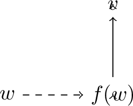
Lemma 5.2. Let \(\mathcal{M}=(W, \leq, f, V)\) be an expanding model and \(w,v \in W\). If \(w \leq v\), then \(f^n(w) \leq f^n(v)\) for all \(n < \omega\).
Proof. By induction on \(n\). For \(n=0\) recall that \(f^0(w) = w \leq v = f^0(v)\). For \(n >0\) we have \(f^{n-1}(w) \leq f^{n-1}(v)\) by induction hypothesis and therefore \(f^n(w) \leq f^n(v)\) by forward confluence. ◻
Lemma 5.3. Let \(\mathcal{M}=(W, \leq, f, V)\) be a persistent model, \(w,v \in W\) and \(n < \omega\). If \(f^n(w) \leq v\), then there exists \(u \in W\) with \(w \leq u\) and \(f^n(u) = v\).
Proof. By induction on \(n\). For \(n= 0\) we have that \(f^0(w) = w \leq v\), so let \(u = v\). For \(n > 0\) since \(f(f^{n-1}(w)) = f^n(w)\) and \(f^n(w) \leq v\), by back-up confluence there exists \(u' \in W\) with \(f^{n-1}(w) \leq u'\) and \(f(u') = v\). By induction hypothesis there exists \(u \in W\) with \(w \leq u\) and \(f^{n-1}(u) = u'\). Thus \(f^n(u) = v\). ◻
Lemma 5.4 (Monotonicity). Let \(\mathcal{M}=(W, \leq, V, f)\) be an expanding (persistent) model, \(w,v \in W\) and \(\varphi\) a formula. If \(\mathcal{M},w \models \varphi\) and \(w \leq v\), then \(\mathcal{M},v \models \varphi\).
Proof. By induction on \(\varphi\). The base cases as well as the cases where \(\varphi = \psi \ast \chi\) for \({\ast \in \{\wedge, \vee, \rightarrow\}}\) follow from Lemma 2.2. The case for \(\varphi = \mathbin{{\bigcirc}}\psi\) follows from Lemma 2.5, Lemma 2.6 and Lemma 2.7. For \(\varphi = \psi \mathbin{\mathsf{U}}\chi\) if \(\mathcal{M}, w \models \psi \mathbin{\mathsf{U}}\chi\), then there exists \(n < \omega\) such that \(f^n(w) \models \chi\) and for all \(0 \leq m < n\), \(\mathcal{M}, f^m(w) \models \psi\). By Lemma 5.2, \(f^k(w) \leq f^k(v)\) for all \(0 \leq k \leq n\). Thus by induction hypothesis \(\mathcal{M}, f^n(v) \models \chi\) and for all \(0 \leq m < n\), \(\mathcal{M}, f^m(v) \models \psi\), implying that \(\mathcal{M}, v \models \psi \mathbin{\mathsf{U}}\chi\). ◻
5.3 Nested Non-Wellfounded Proofs↩︎
This section presents non-wellfounded sequent calculi for \(\mathsf{iLTL}\) over expanding models and over persistent models, respectively. In difference to the non-wellfounded calculus \(\mathrm{nIM}\) for \(\mathsf{IM}\), the systems do not feature a focus annotation. Recall that the focus annotation in \(\mathrm{nIM}\) was used to prove soundness of the cyclic system. Since we only study non-wellfounded systems here, the focus annotation is no longer needed. However, due to the lack of a focus annotation, the global correctness criterion imposed on infinite branches is formulated differently using formula traces. To ensure completeness, the calculi incorporate a simple form of nesting, which is inspired by the work of Kojima and Igarashi [85] who developed a nested sequent calculus for a version of \(\mathsf{iLTL}\) where the only temporal modality is \(\mathbin{{\bigcirc}}\).
Definition 5.5. A nested formula* is a tuple \((\varphi,n)\), denoted by \(\varphi^n\), with \(\varphi \in \mathcal{L}_\mathsf{iLTL}\) and \(n< \omega\). A sequent is an ordered pair \(\Gamma \Rightarrow \Delta\), where \(\Gamma\) and \(\Delta\) are finite sets of nested formulas.*
Note that in difference to the definition of sequents for \(\mathrm{nIM}\), every tuple \(\Gamma \Rightarrow \Delta\) with \(\Gamma, \Delta\) being finite sets of nested formulas is a sequent. As before, we denote sequents by \(\sigma\) and \(\Gamma_\sigma\), \(\Delta_\sigma\) denote the left side and right side of \(\sigma\), respectively. For the remainder of this chapter nested formulas are simply called formulas. Formulas that are not nested are called plain. As for \(\mathrm{nIM}\) we consider multi-conclusion sequents. Once again, this is to simplify the proof search argument in the completeness proof. At first glance, nested formulas might look little different to annotated formulas, but this is misleading. The difference becomes clear in the interpretation of a sequent.
Definition 5.6. The interpretation* of a nested formula \(\varphi^n\) is the plain formula \(\mathbin{{\bigcirc}}^n \varphi\). The interpretation of a sequent \(\sigma\) is the plain formula \[\sigma^I \mathrel{\vcenter{:}}= \bigwedge_{\varphi^n \in \Gamma_\sigma}\mathbin{{\bigcirc}}^{n} \varphi \rightarrow \bigvee_{\psi^m \in \Delta_\sigma} \mathbin{{\bigcirc}}^{m} \psi\]*
To simplify notation, we write \(\mathcal{M},w \models \varphi^n\) if \(M,w \models \mathbin{{\bigcirc}}^n \varphi\) and \(\mathcal{M},w\models \sigma\) if \(M,w \models \sigma^I\). For any set \(\Gamma\) of nested formulas, define \[\Gamma^{+1} \mathrel{\vcenter{:}}= \{\varphi^{n+1}: \varphi^n\in \Gamma\}.\]
We will now introduce the sequent calculi \(\mathrm{niLTL_e}\) and \(\mathrm{niLTL_p}\), which will be proven to be sound and complete with respect to the classes of expanding models and of persistent models, respectively. Both calculi are based on the basic rules depicted in Table 9 as well as some of the additional rules in Table 10.
Definition 5.7. Consider the rules depicted in Table 9 and Table 10.
The sequent calculus \(\mathrm{niLTL_e}\) consists of the basic rules as well as the rules \({\rightarrow} \mathsf{R}\) and \(\mathsf{S}\).
The sequent calculus \(\mathrm{niLTL_p}\) consists of the basic rules as well as the rule \({\rightarrow} \mathsf{R_p}\).
| \(\infer[\mathsf{id}]{ \Gamma, \varphi^n \Rightarrow \varphi^n, \Delta}{}\) | \(\infer[\bot]{\Gamma, \bot^n \Rightarrow \Delta}{}\) |
| \(\infer[\wedge \mathsf{L}]{\Gamma, \varphi \wedge \psi^n \Rightarrow \Delta}{\Gamma, \varphi^n,\psi^n \Rightarrow \Delta}\) | \(\infer[\wedge \mathsf{R}]{\Gamma \Rightarrow \varphi \wedge \psi^n, \Delta}{\Gamma \Rightarrow \varphi^n, \Delta & \Gamma \Rightarrow \psi^n, \Delta}\) |
| \(\infer[\vee \mathsf{L}]{\Gamma, \varphi \vee \psi^n \Rightarrow \Delta}{\Gamma, \varphi^n \Rightarrow \Delta & \Gamma, \psi^n \Rightarrow \Delta}\) | \(\infer[\vee \mathsf{R}]{\Gamma \Rightarrow \varphi \vee \psi^n, \Delta}{\Gamma \Rightarrow \varphi^n,\psi^n, \Delta}\) |
| \(\infer[\X \mathsf{L}]{\Gamma, \X \varphi^{n} \Rightarrow \Delta}{\Gamma, \varphi^{n+1} \Rightarrow \Delta}\) | \(\infer[\X\mathsf{R}]{\Gamma\Rightarrow \X \varphi^{n} \!, \Delta}{\Gamma\Rightarrow \varphi^{n+1} \!, \Delta}\) |
| \(\infer[\U \mathsf{L}]{\Gamma, \varphi \U \psi^n \Rightarrow \Delta}{\Gamma, \psi^n \Rightarrow \Delta & \Gamma, \varphi^n\! ,\X (\varphi \U \psi)^n \Rightarrow \Delta}\) | \(\infer[\U \mathsf{R}]{\Gamma \Rightarrow \varphi \U \psi^n\!, \Delta}{\Gamma\Rightarrow \psi^n\!, \varphi^n\!, \Delta & \Gamma \Rightarrow \psi^n\! , \X (\varphi \U \psi)^n\!, \Delta}\) |
| \(\infer[{\rightarrow} \mathsf{L}]{\Gamma, \varphi \rightarrow \psi^n \Rightarrow \Delta}{\Gamma, \varphi \rightarrow \psi^n \Rightarrow \varphi^n, \Delta & \Gamma, \psi^n \Rightarrow \Delta}\) | |
| \(\infer[{\rightarrow} \mathsf{R}]{\Gamma \Rightarrow \varphi \rightarrow \psi^0, \Delta}{\Gamma, \varphi^0 \Rightarrow \psi^0}\) | \(\infer[{\rightarrow} \mathsf{R_p}]{\Gamma \Rightarrow \varphi \rightarrow \psi^n, \Delta}{\Gamma, \varphi^n \Rightarrow \psi^n}\) |
| \(\infer[\mathsf{S}]{\Sigma, \Gamma^{+1} \Rightarrow \Delta^{+1}, \Pi}{\Gamma \Rightarrow \Delta}\) | |
The rules \(\mathsf{id}\) and \(\bot\) are called axioms. The basic rules for \(\wedge, \vee, \rightarrow\) are nested versions of the corresponding rules in the sequent calculus for intuitionistic logic \(\mathrm{IPL_s}\) (see Definition 2.15). The \(\mathbin{\mathsf{U}}\)-rules capture the equivalence \[\varphi\mathbin{\mathsf{U}}\psi\equiv \psi\lor (\varphi\land \mathbin{{\bigcirc}}(\varphi\mathbin{\mathsf{U}}\psi)).\] Note that the rules \(\mathbin{{\bigcirc}}\mathsf{L}\) and \(\mathbin{{\bigcirc}}\mathsf{R}\) are purely structural as \(\mathbin{{\bigcirc}}\varphi^n\) has the same interpretation as \(\varphi^{n+1}\). Regarding the additional rules observe that the rule \({\rightarrow} \mathsf{R}\) can only be applied to implications with nesting level \(0\) while the rule \({\rightarrow} \mathsf{R_p}\) can be applied to implications of arbitrary nesting level. Interestingly, this is the crucial difference between the calculi \(\mathrm{niLTL_e}\) and \(\mathrm{niLTL_p}\). To understand why, it is instructive to think semantically about what these rules express. Naturally, both rules should preserve validity when read top-down. The rule \({\rightarrow} \mathsf{R_p}\) then expresses that if \(\mathbin{{\bigcirc}}^n \varphi \rightarrow \mathbin{{\bigcirc}}^n \psi\) is valid, so is \(\mathbin{{\bigcirc}}^n (\varphi \rightarrow \psi)\). By Lemma 5.1 this rule preserves validity over persistent models, but not over expanding models. Thus, for \(\mathrm{niLTL_e}\), we must use the standard implication rule, where the nesting level is \(0\). This restriction forces us to include an additional rule for \(\mathrm{niLTL_e}\), namely the ‘shift’-rule \(\mathsf{S}\), that allows us to reduce the nesting level of formulas and captures necessitation. For \(\mathrm{niLTL_p}\), the shift-rule is not required.
Recall the (semantic) definition of an invertible rule (c.f. Definition 3.17). The following lemma is routine.
Lemma 5.5. All basic rules are invertible, while all additional rules are not invertible.
We will therefore refer to the additional rules as the non-invertible rules and to all other rules as the invertible rules.
For each rule, the distinguished formula in the conclusion is called principal and the distinguished formulas in the premises are called its residuals. For \(\mathrm{S}\), all formulas in the conclusion are principal and each formula in the premise is the residual of its corresponding principal formula; in particular, formulas in \(\Sigma\) and \(\Pi\) have no residual. In every rule application, any formula that is neither principal nor residual is called a side formula. For the remainder of this section, let \(\mathsf{P} \in \{\mathrm{niLTL_e}, \mathrm{niLTL_p}\}\).
Definition 5.8. A \(\mathsf{P}\)-pre-proof* of a sequent \(\sigma\) is a finite or infinite tree whose nodes are labeled according to the rules of \(\mathsf{P}\) and whose root is labeled by \(\sigma\).*
Recall the definition of a path through a tree (c.f. Section 2.1). If there is no danger of confusion, paths will be identified with the sequence of sequents that label the nodes of the path.
Definition 5.9. Let \(\rho =(\rho(i))_i\) be a path through a pre-proof \(\pi\). A (formula) trace* on \(\rho\) is a finite or infinite sequence of nested formulas \(\varphi_0^{n_0}, \varphi_1^{n_1},\dots\) such that for each index \(i\) the following hold.*
\(\varphi_i^{n_i}\) occurs on the left side of the sequent labelling \(\rho(i)\);
If \(\varphi_{i}^{n_i}\) is a principal formula in the rule applied at \(\rho(i)\), then \(\varphi_{i+1}^{n_{i+1}}\) is a residual formula of \(\varphi_i^{n_i}\) in \(\rho(i+1)\);
if \(\varphi_{i}^{n_i}\) is a side formula in the rule applied at \(\rho(i)\), then \(\varphi_{i+1}^{n_{i+1}}=\varphi_{i}^{n_i}\).
For any rule \(\mathsf{r}\), a trace \((\varphi_i^{n_i})_{i}\) passes actively through \(\mathsf{r}\) if there is an index \(j\) such that \(\varphi_j^{n_j}\) is a principal formula in an instance of \(\mathsf{r}\). To keep the notation simple, when reasoning about traces \((\varphi_i^{n_i})_i\), we will usually omit the index for the nesting and simply write \((\varphi_i)_i\). It will always be clear from context that we refer to nested formulas and not to plain formulas.
Note that the focus annotation employed in the non-wellfounded system \(\mathrm{nIM}\) in Chapter 3 captures specific formulas traces. Namely a good suffix in a branch of an \(\mathrm{nIM}\)-pre-proof always has a formula in focus which is of the form \(\ooalign{\larger[-1.5]\square\cr \hidewidth\raise.035ex* \mkern 1.12mu\cr}\psi^f\) or \(\larger[-1.5]\square\ooalign{\larger[-1.5]\square\cr \hidewidth\raise.035ex* \mkern 1.12mu\cr}\psi^f\) for some formula \(\psi\). Therefore we obtain a trace through a good suffix by considering the infinite sequence of focused formulas \((\varphi_i)_i\) occurring in the suffix. Note that this sequence satisfies the definition of a formula trace above (minus the first condition, which has to be replaced by the condition that the trace formula (i.e. the formula in focus) occurs on the right side of the sequent). The focus annotation thus keeps track of one trace through a suffix of an infinite branch, and in order for the suffix to be good, it is required that the trace passes infinitely often through an instance of \(\ooalign{\larger[-1.5]\square\cr \hidewidth\raise.035ex* \mkern 1.12mu\cr}\mathsf{R}\). Here, we define similarly the notion of a good trace.
Definition 5.10. A formula trace is good* if it actively passes through infinitely many applications of the rule \(\mathbin{\mathsf{U}}\mathrm{L}\).*
The following lemma describes a straightforward yet key property of good formula traces, where the complexity of a nested formula is simply the complexity of the underlying plain formula. We provide a proof sketch.
Lemma 5.6. If \((\varphi_i)_i\) is a good formula trace, then there is a plain formula of the form \(\varphi\mathbin{\mathsf{U}}\psi\) and some \(k < \omega\) such that for all \(i\geq k\), \(\varphi_i\) is of the form \(\varphi\mathbin{\mathsf{U}}\psi^{n_i}\) or \(\mathbin{{\bigcirc}}(\varphi\mathbin{\mathsf{U}}\psi)^{n_i}\) for \(n_i < \omega\).
Proof Sketch.. Let \((\varphi_i)_i\) be a good formula trace. Then \((\varphi_i)_i\) actively passes through infinitely many applications of the rule \(\mathbin{\mathsf{U}}\mathsf{L}\). Let \((i_j)_j\) be the infinite sequence of natural numbers such that for all \(i < \omega\) the trace formula \(\varphi_{i}\) is principal in an instance of \(\mathbin{\mathsf{U}}\mathsf{L}\) if and only if \(i = i_j\) for some \(j < \omega\). We claim that for all \(j < \omega\), \(c(\varphi_{i_j}) \geq c(\varphi_{i_{j+1}})\). To show this let \(j < \omega\) and consider \(\varphi_{i_j}\) and \(\varphi_{i_{j+1}}\). By assumption \(\varphi_{i_j}\) is of the form \(\varphi \mathbin{\mathsf{U}}\psi^{n_{i_j}}\) for some plain formulas \(\varphi\) and \(\psi\) and \(\varphi_{i_j+1}\) is either \(\psi^{n_{i_j}}\) or \(\varphi^{n_{i_j}}\) or \(\mathbin{{\bigcirc}}(\varphi \mathbin{\mathsf{U}}\psi)^{n_{i_j}}\). By inspection of the rules, note that the only rule that increases the complexity of a trace formula (when read bottom-up) is the rule \(\mathbin{\mathsf{U}}\mathsf{L}\) (recall that trace formulas cannot occur on the right side of a sequent). Since there are no applications of \(\mathbin{\mathsf{U}}\mathsf{L}\) between \(\varphi_{i_j +1}\) and \(\varphi_{i_{j+1}}\), we have \(c(\varphi_{i_j +1}) \geq c(\varphi_{i_{j+1}})\). If \(\varphi_{i_j + 1}\) is \(\varphi^{n_{i_j}}\) or \(\psi^{n_{i_j}}\), then \(c(\varphi_{i_j}) > c(\varphi_{i_{j+1}})\). If \(\varphi_{i_j + 1} = \mathbin{{\bigcirc}}(\varphi \mathbin{\mathsf{U}}\psi)^{n_{i_j}}\), then note that the only rules through which the trace can actively pass through between \(i_j+1\) and \(i_{j+1}\) are instances of \(\mathsf{S}\) and of \(\mathbin{{\bigcirc}}\mathsf{L}\). Note that the trace must actively pass through exactly one instance of \(\mathbin{{\bigcirc}}\mathsf{L}\), implying that \(c(\varphi_{i_j}) = c(\varphi_{i_{j+1}})\). Therefore \((c(\varphi_{i_j}))_{j}\) is an infinite sequence of decreasing natural numbers, which strictly decreases whenever \(\varphi_{i_{j}}\) is the principal formula in an instance of \(\mathbin{\mathsf{U}}\mathsf{L}\) and \(\varphi_{i_j+1} \not = \mathbin{{\bigcirc}}\varphi_{i_j}\). Since natural numbers are well-founded, there exists a natural number \(k\) such that \(c(\varphi_{i_j}) = c(\varphi_{i_{k}})\) for all \(j > k\). Thus the only rules through which the suffix \((\varphi_i)_{i \geq k}\) actively passes through are instances of \(\mathsf{S},\mathbin{{\bigcirc}}\mathsf{L}\) or instances of \(\mathbin{\mathsf{U}}\mathsf{L}\) where if \(\varphi_i\) is principal, then \(\varphi_{i+1} = \mathbin{{\bigcirc}}\varphi_i\). Hence for all \(i \geq k\), \(\varphi_i = \varphi \mathbin{\mathsf{U}}\psi^{n_i}\) or \(\varphi_i = \mathbin{{\bigcirc}}(\varphi \mathbin{\mathsf{U}}\psi)^{n_i}\) for some plain formula \(\varphi \mathbin{\mathsf{U}}\psi\) and \(n_i < \omega\). ◻
Definition 5.11. A \(\mathsf{P}\)-proof* of a sequent \(\sigma\) is a \(\mathsf{P}\)-pre-proof \(\pi\) of \(\sigma\) such that*
every leaf in \(\pi\) is labeled by an axiom;
every infinite branch of \(\pi\) contains a suffix that has a good formula trace.
Example 5.1. The formula \((\mathbin{{\bigcirc}}\varphi \rightarrow \mathbin{{\bigcirc}}\psi) \rightarrow \mathbin{{\bigcirc}}(\varphi \rightarrow \psi)^0\) is provable in \(\mathrm{niLTL_p}\):
Note that the same formula is not provable in \(\mathrm{niLTL_e}\). The lower-most application of \({\rightarrow}\mathsf{R_p}\) can be replaced by an application of \({\rightarrow} \mathsf{R}\), however, the next application of \({\rightarrow}\mathsf{R_p}\) cannot be replaced. If we apply \(\mathsf{S}\), then the formula on the left-hand side is lost and the resulting sequent \(\Rightarrow \varphi \rightarrow \psi^0\) is not provable. If we apply \({\rightarrow}\mathsf{L}\) first, then the resulting right premise \(\mathbin{{\bigcirc}}\psi^0 \Rightarrow \varphi \rightarrow \psi^1\) is provable by applying \(\mathbin{{\bigcirc}}\mathsf{L}\) to \(\mathbin{{\bigcirc}}\psi^0\), \(\mathsf{S}\) and then \({\rightarrow} \mathsf{R}\), but the left premise \(\mathbin{{\bigcirc}}\varphi \rightarrow \mathbin{{\bigcirc}}\psi^0 \Rightarrow \mathbin{{\bigcirc}}\varphi^0, \varphi \rightarrow \psi^1\) is not provable, since \({\rightarrow} \mathsf{R}\) has a single-conclusion premise.
5.4 Soundness↩︎
This section establishes soundness of \(\mathrm{niLTL_e}\) with respect to the class of expanding models and of \(\mathrm{niLTL_p}\) with respect to the class of persistent models. The proof is essentially an infinitary version of the soundness proof for \(\mathrm{cIM}\). The measure \(\mu(\sigma)\) assigned to sequents is generalised to signatures: maps that associate a natural number to each ‘relevant’ formula in a sequent \(\sigma\). We then assume towards a contradiction that there is a proof \(\pi\) of an invalid sequent \(\sigma\) and show, using a countermodel of \(\sigma\), how to find an infinite path \(\rho\) of invalid sequents in \(\pi\) such that their signatures never increase but strictly decrease infinitely often, thus obtaining a contradiction to the well-foundedness of the natural numbers. The aforementioned ‘relevant’ formulas are called eventualities.
Definition 5.12. An eventuality* is a formula of the form \(\mathbin{{\bigcirc}}^j (\varphi\mathbin{\mathsf{U}}\psi)^n\) with \(n,j < \omega\). Given a sequent \(\sigma\), a formula \(E\) is an eventuality of \(\sigma\) if \(E\) is an eventuality occurring in \(\Gamma_\sigma\).*
Let \(\mathbin{\mathsf{U}}^k\) be the operator defined inductively by \(\varphi\mathbin{\mathsf{U}}^0 \psi=\psi\) and \(\varphi\mathbin{\mathsf{U}}^{k+1}\! \psi=\varphi\land \mathbin{{\bigcirc}}(\varphi\mathbin{\mathsf{U}}^{k}\! \psi)\). For an eventuality \(E=\mathbin{{\bigcirc}}^j (\varphi\mathbin{\mathsf{U}}\psi)^n\) and \(k < \omega\) define \[\begin{align} E[k]:=\mathbin{{\bigcirc}}^j (\varphi\mathbin{\mathsf{U}}^{k}\! \psi)^n. \end{align}\] Given a sequent \(\sigma\), a signature for \(\sigma\) is a map \(\tau\) which assigns a natural number to each eventuality of \(\sigma\). Let \(\Gamma_\sigma[\tau]\) be the set obtained from \(\Gamma_\sigma\) by replacing each eventuality \(E\) with \(E[\tau(E)]\). Furthermore, let \(\sigma[\tau]\) denote the sequent \(\Gamma_\sigma[\tau]\Rightarrow \Delta_\sigma\).
Lemma 5.7. Let \(\mathcal{M}=(W, \leq, f, V)\) be an expanding (persistent) model and \(E\) an eventuality. Then \(\mathcal{M}, w \models E\) if and only if there exists a natural number \(k\) such that \(\mathcal{M}, w \models E[k]\).
Proof. Let \(E\) be an eventuality, \(\mathcal{M}=(W, \leq, f, V)\) an expanding (persistent) model and \(w \in W\) a world with \(\mathcal{M}, w \models E\). There are formulas \(\varphi, \psi\) and natural numbers \(j,n\) such that \(E = \mathbin{{\bigcirc}}^j (\varphi \mathbin{\mathsf{U}}\psi)^n\). If \(\mathcal{M}, w \models E\), then \(\mathcal{M}, f^{j+n}(w) \models \varphi \mathbin{\mathsf{U}}\psi\). By definition there exists a natural number \(k\) such that for all \(j+n \leq i < k\) holds that \(\mathcal{M}, f^i(w) \models \varphi\) and \(\mathcal{M}, f^k(w) \models \psi\). Hence \(\mathcal{M}, f^{n+j}(w) \models \mathbin{{\bigcirc}}^i \varphi\) for all \(i < k -(j +n)\) and so \(\mathcal{M}, f^{j+n}(w) \models \varphi \mathbin{\mathsf{U}}^k \psi\). Thus \(\mathcal{M}, w \models \mathbin{{\bigcirc}}^j (\varphi \mathbin{\mathsf{U}}^k \psi)^n\). For the other direction suppose there exists a natural number \(k\) such that \(\mathcal{M}, w \models E[k]\). So \(\mathcal{M}, f^{j+n}(w) \models \varphi \mathbin{\mathsf{U}}^k \psi\). An induction on \(k\) shows that \(\mathcal{M}, f^{j+n}(w) \models \varphi \mathbin{\mathsf{U}}\psi\). The proof is routine. Hence \(\mathcal{M}, w \models E\). ◻
Note that Lemma 5.7 implies that given \(\mathcal{M}, w\) and \(E\) with \(\mathcal{M}, w \models E\), there exists a least natural number \(k\) with \(\mathcal{M}, w \models E[k]\).
Theorem 5.2 (Soundness for \(\mathrm{niLTL_e}\)). Every sequent provable in \(\mathrm{niLTL_e}\) is valid over the class of expanding models.
Proof. Let \(\pi\) be an \(\mathrm{niLTL_e}\)-proof of \(\sigma\) and suppose, for contradiction, that \(\sigma\) is not valid. Let \(\mathcal{M}=(W,\leq,f,V)\) be an expanding model and \(w\in W\) such that \(\mathcal{M},w\not\models\sigma\). For brevity, we will identify each node in \(\pi\) with the sequent that labels it.
We will inductively define an infinite path \((\sigma_i)_i\) of sequents through \(\pi\), an infinite sequence of worlds \((w_i)_i\) in \(\mathcal{M}\) and an infinite sequence of signatures \((\tau_i)_i\) such that the following hold for every \(i < \omega\):
\(\tau_i\) is a signature for \(\sigma_i\);
\(w_i\models \bigwedge \Gamma_{\sigma_i}[\tau_i]\) and \(w_i\not\models \bigvee \Delta_{\sigma_i}\) (thus \(w_i\not\models \sigma_i[\tau_i]\) and so by Lemma 5.7, \(w_i\not\models \sigma_i\));
for every eventuality \(E\) of \(\sigma_i\), the following hold:
\(\tau_i(E)\) is the least natural number \(k\) such that \(w_i\models E[k]\);
if \(E\) is a side formula in the rule application with conclusion \(\sigma_i\), then \(E\) is an eventuality of \(\sigma_{i+1}\) and \(\tau_{i+1}(E)\leq\tau_i(E)\).
We define \((\sigma_i)_i\), \((w_i)_i\) and \((\tau_i)_i\) by induction on \(i\) as follows.
Set \(\sigma_0=\sigma\). Since \(w\not\models \sigma\), there exists a \(v\geq w\) such that \(v\models \bigwedge \Gamma_\sigma\) and \(v\not\models \bigvee \Delta_\sigma\). Set \(w_0=v\) and for every eventuality \(E\) in \(\Gamma_\sigma\), define \(\tau_0(E)\) to be the least \(k\) such that \(w_0 \models E[k]\) (which exists by Lemma 5.718). Note that by construction \((\sigma_0,w_0, \tau_0)\) satisfies the properties 1. – 3.
Suppose \(\sigma_i, w_i\) and \(\tau_i\) are given and satisfy the properties 1. – 3. To define \(\sigma_{i+1}, w_{i+1}\) and \(\tau_{i+1}\) we use a case distinction based on the rule applied at \(\sigma_i\) in \(\pi\) (i.e. the rule that has \(\sigma_i\) as conclusion). Note that this rule cannot be an axiom, since \(w_i\not\models \sigma_i\) and it is straightfoward to check that the conclusion of every instance of an axiom is valid. Case for \(\wedge \mathsf{L}\). Suppose \(\sigma_i = (\Gamma, \varphi \wedge \psi^n \Rightarrow \Delta)\) with \(\varphi \wedge \psi^n\) principal in the rule application. By assumption \(w_i \models \varphi \wedge \psi^n\), implying that \(f^n(w_i) \models \varphi \wedge \psi\). Hence \(f^n(w_i) \models \varphi\) and \(f^n(w_i) \models \psi\) and so \(w_i \models \varphi^n\) and \(w_i \models \psi^n\). Let \(\sigma_{i+1} \mathrel{\vcenter{:}}= (\Gamma, \varphi^n, \psi^n \Rightarrow \Delta)\) and \(w_{i+1} = w_i\). If \(\varphi^n\) or \(\psi^n\) is an eventuality, define \(\tau_{i+1}(\varphi^n)\) to be the least natural number \(k\) such that \(w_{i+1} \models \varphi^n[k]\) and similarly for \(\tau_{i+1}(\psi^n)\). On all other eventuality \(E\), let \(\tau_{i+1}(E) \mathrel{\vcenter{:}}= \tau_i(E)\). Note that the properties 1. – 3. hold.
Case for \(\wedge \mathsf{R}\). Suppose \(\sigma_i = (\Gamma \Rightarrow \varphi \wedge \psi^n, \Delta)\) with \(\varphi \wedge \psi^n\) principal in the rule application. By assumption \(w_i \not \models (\varphi \wedge \psi^n)\), implying that \(f^n(w_i) \not \models \varphi \wedge \psi\). Thus \(f^n(w) \not \models \varphi\) or \(f^n(w) \not \models \psi\), so \(w_i \not \models \varphi^n\) or \(w_i \not \models \psi^n\). If \(w_i \not \models \varphi^n\), let \(\sigma_{i+1} \mathrel{\vcenter{:}}= (\Gamma \Rightarrow \varphi^n, \Delta)\), \(w_{i+1} \mathrel{\vcenter{:}}= w_i\) and \(\tau_{i+1} \mathrel{\vcenter{:}}= \tau_i\). Note that the properties 1. – 3. hold. The case where \(w_i \not \models \psi^n\) is similar by choosing the sequent in the right premise of \(\wedge \mathsf{R}\) as \(\sigma_{i+1}\).
Cases for \(\vee \mathsf{L}\) and \(\vee \mathsf{R}\). The cases for \(\vee \mathsf{L}\) and \(\vee \mathsf{R}\) are symmetric to the cases for \(\wedge \mathsf{R}\) and for \(\wedge \mathsf{L}\), respectively.
Case for \({\rightarrow} \mathsf{L}\). Suppose \(\sigma_i = (\Gamma, \varphi \rightarrow \psi^n \Rightarrow \Delta)\) and \(\varphi \rightarrow \psi^n\) is principal in the rule application. By assumption \(w_i \models \varphi \rightarrow \psi^n\), implying that \(f^n(w_i) \models \varphi \rightarrow \psi\). If \(f^n(w_i) \not \models \varphi\), then \(w_i \not \models \varphi^n\) and so let \(\sigma_{i+1} \mathrel{\vcenter{:}}= (\Gamma, \varphi \rightarrow \psi^n \Rightarrow \varphi^n, \Delta)\), \(w_{i+1} \mathrel{\vcenter{:}}= w_i\) and \(\tau_{i+1} \mathrel{\vcenter{:}}= \tau_i\). Note that the properties 1. – 3. are satisfied. Otherwise \(f^n(w_i) \models \psi\), implying that \(w_i \models \psi^n\). Hence let \(\sigma_{i+1} \mathrel{\vcenter{:}}= (\Gamma, \psi^n \Rightarrow \Delta)\), \(w_{i+1} \mathrel{\vcenter{:}}= w_i\) and if \(\psi^n\) is an eventuality, let \(\tau_{i+1}(\psi^n)\) be the least natural number \(k\) such that \(w_{i+1} \models \psi^n[k]\). On all other eventualities \(E\), \(\tau_{i+1}(E) \mathrel{\vcenter{:}}= \tau_i(E)\). Note that the properties 1. – 3. are satisfied.
Case for \({\to} \mathrm{R}\). Suppose \(\sigma_i= (\Gamma \Rightarrow \varphi\rightarrow \psi^0,\Delta)\) with \(\varphi\rightarrow \psi^0\) principal in the rule application. Let \(\sigma_{i+1}=(\Gamma, \varphi^0\Rightarrow \psi^0)\). Since \(w_i \not \models \varphi \rightarrow \psi^0\), there exists a \(v \geq w_i\) such that \(v \models \varphi^0\) and \(v\not\models \psi^0\). Let \(w_{i+1} = v\). For any eventuality \(E\) in \(\Gamma\cup\{\varphi^0\}\), let \(\tau_{i+1}\) map \(E\) to the least \(k\) such that \(w_{i+1}\models E[k]\). Note that \(\tau_{i+1}\) is a well-defined signature for \(\sigma_{i+1}\). Moreover, by construction, the properties 2. and 3.(a) hold. Since \(w_{i+1}\geq w_i\), by monotonicity (Lemma 5.4) we have \(\tau_{i+1}(E)\leq \tau_{i}(E)\) for each eventuality \(E\) in \(\Gamma\), implying that 3.(b) holds as well.
Case for \(\mathbin{{\bigcirc}}\mathrm{L}\). Suppose \(\sigma_i= (\Gamma, \mathbin{{\bigcirc}}\varphi^n\Rightarrow \Delta)\) with \(\mathbin{{\bigcirc}}\varphi^n\) principal in the rule application. Let \(\sigma_{i+1}=(\Gamma, \varphi^{n+1}\Rightarrow \Delta)\) and \(w_{i+1}=w_i\). If \(\varphi^{n+1}\) is an eventuality, then define \({\tau_{i+1}(\varphi^{n+1})\mathrel{\vcenter{:}}= \tau_i(\mathbin{{\bigcirc}}\varphi^n)}\). For any other eventuality \(E\), let \(\tau_{i+1}(E) \mathrel{\vcenter{:}}= \tau_i(E)\). Note once again that the properties 1.-3. hold. In particular, the formula \(\varphi^{n+1}\) has the same interpretation as \(\mathbin{{\bigcirc}}\varphi^n\), implying that \(\tau_{i+1}(\varphi^{n+1})\) is the least \(k\) such that \(w_{i+1} \models \varphi^{n+1}[k]\).
Case for \(\mathrm{S}\). Suppose \(\sigma_i= (\Sigma,\Gamma^{+1} \Rightarrow \Delta^{+1},\Pi)\) such that \(\Gamma \Rightarrow \Delta\) is the premise of the rule application. Let \(\sigma_{i+1}=(\Gamma \Rightarrow \Delta)\), \(w_{i+1}=f(w_i)\) and \(\tau_{i+1}(E^n)=\tau_i(E^{n+1})\) for every eventuality \(E^n\) in \(\Gamma\). By construction \(\tau_{i+1}\) is a signature. Note that since \(w_i \models \Gamma^{+1}_{\sigma_i}[\tau_i]\), it holds that \(f(w_i) \models \Gamma_{\sigma_i}[\tau_{i+1}]\). Therefore the property 2. holds as well. Property 3.(b) is given by construction, while 3.(a) holds since if there would exists a natural number \(k < \tau_{i+1}[E]\) with \(w_{i+1} \models E[k]\) for some eventuality \(E\) in \(\Gamma\), then \(w_i \models E^{+1}[k]\), implying that \(\tau_i\) does not satisfy property 3.(a); a contradiction.
Case for \(\mathbin{\mathsf{U}}\mathrm{L}\). Suppose \(\sigma_i= (\Gamma, \varphi\mathbin{\mathsf{U}}\psi^n\Rightarrow \Delta)\) with \(\varphi\mathbin{\mathsf{U}}\psi^n\) principal in the rule application. We distinguish two cases.
If \(\tau_i(\varphi\mathbin{\mathsf{U}}\psi^n)=0\), let \(\sigma_{i+1}=(\Gamma, \psi^n\Rightarrow \Delta)\) and \(w_{i+1}=w_i\). If \(\psi^n\) is an eventuality and not in \(\Gamma\), let \(\tau_{i+1}\) map \(\psi^n\) to the least \(k\) such that \(w_{i+1}\models \psi^n[k]\). On other eventualities, \(\tau_{i+1}\) acts as \(\tau_i\). Clearly, \(\tau_{i+1}\) is a signature. Note that since \(\tau_i(\varphi \mathbin{\mathsf{U}}\psi^n) = 0\), we have \(f^n(w_i) \models \psi\) since \(\varphi \mathbin{\mathsf{U}}^0 \psi = \psi\). Thus the property 2. holds. Properties 3. (a) and (b) hold by construction.
If \(\tau_i(\varphi\mathbin{\mathsf{U}}\psi^n)>0\), let \(\sigma_{i+1}=(\Gamma, \varphi^n, \mathbin{{\bigcirc}}(\varphi\mathbin{\mathsf{U}}\psi)^n\Rightarrow \Delta)\) and \(w_{i+1}=w_i\). If \(\varphi^n\) is an eventuality and not in \(\Gamma\), let \(\tau_{i+1}\) map \(\varphi^n\) to the least \(k\) such that \(w_{i+1}\models \varphi^n[k]\). Define \(\tau_{i+1}(\mathbin{{\bigcirc}}(\varphi\mathbin{\mathsf{U}}\psi)^n) \mathrel{\vcenter{:}}= \tau_i(\varphi\mathbin{\mathsf{U}}\psi^n)-1\). On other eventualities, \(\tau_{i+1}\) acts as \(\tau_i\). By construction the properties 1. and 3.(b) hold. Note that since \(w_i \models \varphi \mathbin{\mathsf{U}}\psi^n[k]\) where \(k = \tau_i(\varphi\mathbin{\mathsf{U}}\psi^n)\), we have that \(w_{i+1} \models \mathbin{{\bigcirc}}(\varphi \mathbin{\mathsf{U}}\psi)^n[k-1]\), and \(k-1\) is the least natural number with this property. Thus we obtain that the properties 2. and 3.(a) hold as well.
Therefore we obtain \((\sigma_i)_i\), \((w_i)_i\) and \((\tau_i)_i\) satisfying the properties 1. – 3. Since \(\pi\) is a proof, the infinite branch \((\sigma_i)_i\) must contain a good trace \((\varphi_i)_{i \geq j}\) starting in some sequent \(\sigma_j\). By Lemma 5.6, we may assume that this trace only passes actively through the rules \(\mathbin{{\bigcirc}}\mathrm{L}\), \(\mathrm{S}\) and \(\mathbin{\mathsf{U}}\mathrm{L}\), and it cannot pass through the latter in a degenerative way.19 Now consider the infinite sequence \((\tau_i(\varphi_i))_{i \geq j}\) of natural numbers. Note that, by property 3(b), if \(\varphi_i\) is a side formula then \(\tau_{i+1}(\varphi_{i+1})\leq \tau_{i}(\varphi_{i})\). Moreover, if \(\varphi_i\) is principal in an application of \(\mathbin{{\bigcirc}}\mathrm{L}\) or \(\mathrm{S}\) then \(\tau_{i+1}(\varphi_{i+1})= \tau_{i}(\varphi_{i}),\) and if \(\varphi_i\) is principal in a (non-degenerative) application of \(\mathbin{\mathsf{U}}\mathrm{L}\) then \(\tau_{i+1}(\varphi_{i+1})<\tau_{i}(\varphi_{i})\) by construction. As the trace is good, the latter case occurs infinitely often, and so we obtain an infinite, strictly decreasing sequence of natural numbers and thereby a contradiction. ◻
We finish the section by proving that \(\mathrm{niLTL_p}\) is sound with respect to the class of persistent models. The proof follows the same argument as for \(\mathrm{niLTL_e}\), with the only differences that the case for \(\mathsf{S}\) can be skipped and the case for \({\rightarrow}\mathsf{R}\) must be replaced by the case for \({\rightarrow}\mathsf{R_p}\).
Theorem 5.3 (Soundness for \(\mathrm{niLTL_p}\)). Every sequent provable in \(\mathrm{niLTL_p}\) is valid over the class of persistent models.
Proof. Let \(\pi\) be an \(\mathrm{niLTL_p}\)-proof of \(\sigma\) and suppose towards contradiction that \(\sigma\) is not valid. Let \(\mathcal{M}=(W, \leq, f, V)\) be a persistent model and \(w \in W\) such that \(\mathcal{M}, w \not \models \sigma\). As in the soundness proof for \(\mathrm{niLTL_e}\) we define inductively a path \((\sigma_i)_i\) of sequents through \(\pi\), a sequence of worlds \((w_i)_i\) in \(\mathcal{M}\) and a sequence of signatures \((\tau_i)_i\) such that the properties 1. - 3. in the proof of Theorem 5.2 hold. We consider the only new case. All other cases are identical to the cases shown above.
Case for \({\rightarrow}\mathsf{R_p}\). Suppose \(\sigma_i = (\Gamma \Rightarrow \varphi \rightarrow \psi^n, \Delta)\) with \(\varphi \rightarrow \psi^n\) principal in the rule application. Let \(\sigma_{i+1} = (\Gamma, \varphi^n \Rightarrow \psi^n)\). Since \(w_i \not \models \varphi \rightarrow \psi^n\), it holds that \(f^n(w_i) \not \models \varphi \rightarrow \psi\). Hence there exists \(v \geq f^n(w_i)\) with \(v \models \varphi\) and \(v \not \models \psi\). By Lemma 5.3 we find a world \(u \geq w_i\) such that \(v = f^n(u)\). Then \(u \models \varphi^n\) and \(u \not \models \psi^n\). Let \(w_{i+1}=u\). It is straightforward to check that \(w_{i+1} \models \bigwedge\Gamma \wedge \varphi^n\) and \(w_{i+1} \not \models \psi^n\). Let \(\tau_{i+1}\) be the signature obtained by mapping each eventuality \(E\) in \(\Gamma \cup \{\varphi^n\}\) to the least natural number \(k\) such that \(w_{i+1} \models E[k]\). From monotonicity (Lemma 5.4) then follows that \(\tau_{i+1}(E) \leq \tau_i(E)\) for each eventuality \(E\) in \(\Gamma \cup \{\varphi^n\}\).
A contradiction to the wellfoundnedness of the natural numbers is now obtained by the same argument as given in the proof of Theorem 5.2 ◻
5.5 Completeness↩︎
This section establishes completeness of \(\mathrm{niLTL_e}\) with respect to the class of expanding models and of \(\mathrm{niLTL_p}\) with respect to the class of persistent models. As for \(\mathrm{nIM}\) the proof proceeds via a proof search argument. For each sequent \(\sigma\) we construct an infinite two-player game between Prover and Refuter such that a winning strategy for Prover corresponds to a proof of \(\sigma\) and a winning strategy for Refuter to the existence of a countermodel for \(\sigma\). The game will be played on a proof search tree, which is a finitely branching, non-wellfounded tree that presents a systematic search for a proof of \(\sigma\). The presented completeness proofs share many similarities with the completeness proof for \(\mathrm{nIM}\). However, there are some crucial differences, due to the presence of forward and back-up confluence, that the countermodels induced by a refutation must satisfy.20 For \(\mathrm{nIM}\), when a formula \(\ooalign{\larger[-1.5]\square\cr \hidewidth\raise.035ex* \mkern 1.12mu\cr}\varphi\) was present on the right side of a sequent, it sufficed to unfold it once to saturate the formula, i.e. it was enough to guarantee that \(\ooalign{\larger[-1.5]\square\cr \hidewidth\raise.035ex* \mkern 1.12mu\cr}\varphi\) was locally correct in the world corresponding to the saturated sequent. In the presence of forward confluence, this does not suffice. Suppose for example that a formula of the form \(\Diamond(\varphi \vee \psi)^0\) (i.e. \(\top \mathbin{\mathsf{U}}(\varphi \vee \psi)^0\)) occurs on the left side of a sequent \(\sigma\) corresponding to the world \(w\). The countermodel then must contain a temporal successor \(f^n(w)\) which satisfies \(\varphi \vee \psi\), which will be guaranteed by the fact that no infinite branch in a refutation can contain a good trace, i.e. after finitely many times unfolding \(\Diamond(\varphi \vee \psi)\) the Refuter must chose the left premise of \(\mathbin{\mathsf{U}}\mathsf{L}\), which will result in the corresponding world satisfying \(\varphi \vee \psi^0\). Saturation then guarantees that \(\varphi^0\) or \(\psi^0\) is contained on the left side of the saturated sequent, implying that the corresonding world \(f^n(w)\) satisfies \(\varphi\) or \(\psi\). However if there exists a world \(v \geq w\), then by forward confluence \(f^n(v) \geq f^n(w)\), so by monotonicity \(f^n(v)\) must satisfy the same disjunct as \(f^w(v)\). In the way proof search trees are defined, the finite segment in a branch corresponding to \(f^n(v)\) is unrelated to the finite segment corresponding to \(f^n(w)\) in the proof search tree. Thus it could happen that at the segment corresponding to \(f^n(w)\), when we apply \(\vee \mathsf{L}\) to \(\varphi \vee \psi^0\), Refuter chooses \(\varphi\), while at the segment corresponding \(f^n(v)\), Refuter chooses \(\psi\), implying that the resulting model is not monotone. To circumvent this problem, we will make use of the nesting and impose that in order to saturate a sequent, we must apply \(\mathbin{\mathsf{U}}\mathsf{L}\) finitely many times until the left premise is chosen, implying that some branches (namely those containing a good trace) will never encounter a saturated sequent. The nesting is crucial for this, as we are able to continue unfolding by eliminating \(\mathbin{{\bigcirc}}\)-operators and instead increase the nesting level.
5.5.1 Completeness for Expanding Models↩︎
We start by giving a suitable notion of saturated sequent.
Definition 5.13. A sequent \(\Gamma\Rightarrow \Delta\) is left-saturated* if the following hold.*
if \(\varphi\land \psi^n\in \Gamma\), then \(\varphi^n,\psi^n\in\Gamma\);
if \(\varphi\lor \psi^n\in \Gamma\), then \(\varphi^n\in\Gamma\) or \(\psi^n\in\Gamma\);
if \(\varphi\to \psi^n\in \Gamma\), then \(\varphi^n\in\Delta\) or \(\psi^n\in\Gamma\);
if \(\mathbin{{\bigcirc}}\varphi^n\in \Gamma\), then \(\varphi^{n+1}\in\Gamma\);
if \(\varphi\mathbin{\mathsf{U}}\psi^n\in \Gamma\), then there exists an \(m\geq n\) such that \(\psi^m\in\Gamma\) and \(\varphi^k\in \Gamma\) for all \(n\leq k< m\).
The sequent is saturated* if, in addition,*
if \(\varphi\land \psi^n\in \Delta\), then \(\varphi^n\in\Delta\) or \(\psi^n\in\Delta\);
if \(\varphi\lor \psi^n\in \Delta\), then \(\varphi^n,\psi^n\in\Delta\);
if \(\mathbin{{\bigcirc}}\varphi^n\in \Delta\), then \(\varphi^{n+1}\in\Delta\);
if \(\varphi\mathbin{\mathsf{U}}\psi^0\in \Delta\), then \(\psi^0,\varphi^0\in\Delta\) or \(\psi^0,\mathbin{{\bigcirc}}(\varphi\mathbin{\mathsf{U}}\psi)^0\in\Delta\).
Given a sequent \(\sigma\), we say that a formula \(\varphi\) is saturated in \(\sigma\)* if \(\sigma\) satisfies the relevant saturation clause for \(\varphi\).*
Note that the saturation clause for right \(\mathbin{\mathsf{U}}\)-formulas is restricted to the zeroth nesting level. As before, we call an application of a rule succinct if the principal formula(s) is not also a side formula, and preserving if the principal formula(s) is also a side formula. Note that rule applications of \({\to} \mathrm{R}\) and \(\mathrm{S}\) are always succinct.
Definition 5.14. A proof search tree* \(\mathcal{T}\) for a sequent \(\sigma\) is a finite or infinite tree whose nodes are labeled according to the rules of \(\mathrm{niLTL_e}\) and in which the following holds.*
The root of \(\mathcal{T}\) is labeled by \(\sigma\).
A node of \(\mathcal{T}\) is a leaf if and only if it is labeled by an axiom.
Every left rule application is succinct.
Every right rule application except \({\to} \mathrm{R}\) is preserving.
No invertible rule is applied to a sequent in which the principal formula is already saturated.
Instead of the rules \({\to} \mathrm{R}\) and \(\mathrm{S}\), we have the rule \[\begin{align} \infer[\mathsf{C},]{\Sigma,\Gamma^{+1}\Rightarrow (\varphi_0\to \psi_0)^{0},\dots,(\varphi_k\to \psi_k)^{0},\Delta^{+1}, \Pi}{\Sigma,\Gamma^{+1}, \varphi_0^{0} \Rightarrow \psi_0^{0} &\dots&\Sigma,\Gamma^{+1}, \varphi_k^{0} \Rightarrow \psi_k^{0}& \Gamma \Rightarrow \Delta} \end{align}\] where it is required that every formula in \(\Sigma\cup \Pi\) is of nesting level \(0\), \(\Pi\) does not contain a formula of the form \(\varphi\to \psi^0\) and the conclusion is a saturated sequent. We call the premises of the form \(\Sigma,\Gamma^{+1}, \varphi_i^0 \Rightarrow \psi_i^0\) the intuitionistic premises, and \(\Gamma\Rightarrow \Delta\) the modal premise* of \(\mathsf{C}\).*
The choice rule \(\mathsf{C}\) represents a choice between non-invertible rules that Prover has to make once the sequent is saturated. Note that the empty sequent is saturated; an empty sequent in a proof search tree can only be the conclusion of a \(\mathrm{C}\)-rule and has another empty sequent as its only direct successor. This is why, in difference to proof search trees for \(\mathrm{nIM}\), every leaf in a proof search tree is labeled by an axiom.
Lemma 5.8. Every sequent \(\sigma\) has a proof search tree.
Intuitively, given a sequent \(\sigma\), one can build a proof search tree as follows. First try to saturate all left formulas by succinctly applying invertible left rules. If a left-saturated sequent is obtained, saturate all right formulas by preservingly applying invertible right rules, then apply \(\mathsf{C}\) and start over. Observe that it is possible that some branches in a proof search tree do not contain a saturated sequent due the fifth saturation clause. The proof is similar to the proof of Lemma 3.26 and omitted.
The following lemmas describe some key properties of proof search trees. For a node \(s\) in a proof search-tree we write \(\Gamma_s\Rightarrow \Delta_s\) to denote the sequent labelling the node \(s\).
Lemma 5.9. If \(\mathcal{T}\) is a proof search tree wherein \(s\in \mathcal{T}\) is the conclusion of a \(\mathsf{C}\)-application with modal premise \(t\in \mathcal{T}\), then the following hold.
\(t\) is labeled by a left-saturated sequent;
if \(r\geq t\) and no \(\mathsf{C}\)-application occurs between \(t\) and \(r\), then \(\Gamma_r=\Gamma_t\).
Proof. Let \(\Gamma_s \Rightarrow \Delta_s = \Sigma,\Gamma^{+1}\Rightarrow (\varphi_0\to \psi_0)^{0},\dots,(\varphi_k\to \psi_k)^{0},\Delta^{+1}, \Pi\) and let \(\Gamma_t \Rightarrow \Delta_t = \Gamma \Rightarrow \Delta\). That \(\Gamma_t \Rightarrow \Delta_t\) is left-saturated follows directly from \(\Gamma_s \Rightarrow \Delta_s\) being left-saturated: note that formulas in \(\Sigma\) are of nesting level \(0\) while each formula in \(\Gamma^{+1}\) is of nesting level strictly larger than \(0\). Hence for any formula in \(\Gamma^{+1}\) its saturation clause is satisfied by formulas in \(\Gamma^{+1}\) and so \(\Gamma_t \Rightarrow \Delta_t\) is left-saturated. Suppose \(r \geq t\) and no \(\mathsf{C}\)-application occurs between \(t\) and \(r\). By 1. \(\Gamma_t\) is labeled by a left-saturated sequent. By Property 5. of a proof search tree no invertible rule is applied to a sequent in which the principal formula is already saturated. Furthermore, the only rule introducing new formulas on the left side of the sequent is \({\rightarrow}\mathsf{R}\), which is merged into the \(\mathsf{C}\)-rule. Therefore no rules can be applied to formulas in \(\Gamma_s\) for any node \(s\) between \(t\) and the next node labeled by the conclusion of a \(\mathrm{C}\)-rule application. Therefore \(\Gamma_t = \Gamma_r\). ◻
Lemma 5.10. Every infinite branch of a proof search tree \(\mathcal{T}\) contains infinitely many applications of \(\mathbin{\mathsf{U}}\mathsf{L}\) or \(\mathsf{C}\).
Proof. Let \((\rho_i)_{i}\) be an infinite branch of \(\mathcal{T}\). Suppose there exists a suffix \((\rho_i)_{i \geq j}\) that contains no applications of \(\mathbin{\mathsf{U}}\mathsf{L}\) or \(\mathsf{C}\). Due to Properties 3. to 5. of the proof search tree, there exists a \(k\geq j\) such that all formulas except for left \(\mathbin{\mathsf{U}}\)-formulas will be saturated in \(\rho_k\). The only rules which may be applied at that point are \(\mathbin{\mathsf{U}}\mathsf{L}\) or \(\mathsf{C}\), showing that \((\rho_i)_{i}\) must be finite. ◻
Lemma 5.11. Every infinite branch of a proof search tree \(\mathcal{T}\) that contains only finitely many \(\mathsf{C}\)-applications has a suffix with a good formula trace.
Proof. Let \(\beta\) be an infinite branch of \(\mathcal{T}\) with finitely many \(\mathsf{C}\)-applications. Let \(\rho\) be a suffix of \(\beta\) that starts after the last \(\mathsf{C}\)-application. By the previous lemma, \(\rho\) must contain infinitely many applications of \(\mathbin{\mathsf{U}}\mathrm{L}\). We show that \(\rho\) contains a good trace.
Consider the tree \(\mathcal{T}_{\rho}\) of formula traces on \(\rho\) (add a fresh node as the root). Now let \(\mathcal{T}'_{\rho}\) be the tree obtained from \(\mathcal{T}_\rho\) by identifying consecutive nodes that are labeled by the same formula. Note that \(\mathcal{T}'_\rho\) cannot be finite, since \(\rho\) must contain infinitely many applications of \(\mathbin{\mathsf{U}}\mathsf{L}\) and this rule may not be applied to formulas that also function as a side formula. Moreover, by inspection of the rules note that \(\mathcal{T}'_\rho\) is finitely branching. By König’s Lemma, \(\mathcal{T}'_\rho\) contains an infinite branch. Note that this branch corresponds to an infinite formula trace \((\varphi_i)_{i}\) on \(\rho\) that does not stagnate on a side formula, that is, \((\varphi_i)_{i}\) actively passes through a left rule infinitely often. Since left rules are applied succinctly and there are no \(\mathsf{C}\)-applications in \(\rho\), the trace \((\varphi_i)_{i}\) must actively passes through \(\mathbin{\mathsf{U}}\mathsf{L}\) infinitely often, implying that \((\varphi_i)_i\) is a good trace. ◻
Next we define proof search games. As before, proof search games are played on proof search trees by two players called Prover and Refuter. Since only one frame condition is considered (and therefore only one choice rule is needed), the choice rule \(\mathsf{C}\) is not displayed in the name of the proof search game.
Definition 5.15. Let \(\sigma\) be a sequent and \(\mathcal{T}\) a proof search tree for \(\sigma\). The proof search game \(\mathcal{G}(\mathcal{T}, \sigma)\) is played by two players called Prover* and Refuter. The arena is the proof search tree \(\mathcal{T}\), where each position is a node of \(\mathcal{T}\). Prover owns every position \(t \in \mathcal{T}\) which is labeled by the conclusion of a \(\mathsf{C}\)-rule instance. Refuter owns every other position. The admissible moves are as follows: if Player owns position \(t\), then Player plays by choosing any child node of \(t\) (if one exists). A play is a sequence of positions \((t_i)_i\) starting in the root of \(\mathcal{T}\) such that any two consecutive positions are related by an admissible move. A play is either finite and ends in a leaf of \(\mathcal{T}\) or infinite. The winning conditions are as follows:*
Prover wins a play \((t_i)_i\) if the play is finite or if it is infinite and \((t_i)_i\) contains a good trace.
Refuter wins a play \((t_i)_i\) if the play is infinite and does not contain a good trace.
Observe that every play in \(\mathcal{G}(\mathcal{T}, \sigma)\) corresponds to a branch of \(\mathcal{T}\). As for \(\mathrm{nIM}\) a strategy for Player is a partial function \(f\) which maps any position \(t\) owned by Player onto a child node of \(t\). Player uses strategy \(f\) if whenever a play is in position \(t\) owned by Player, then Player chooses \(f(t)\). A strategy \(f\) is a winning strategy if Player wins every play in which \(f\) is used. The strategy tree of a strategy \(f\) is the subtree of \(\mathcal{T}\) consisting of all plays that can occur when Player uses \(f\). For detailed definitions, see Definition 3.29, Definition 3.30 and Definition 3.31. The following lemma then follows directly from the winning conditions of Prover.
Lemma 5.12. Suppose Prover has a winning strategy in \(\mathcal{G}(\mathcal{T},\sigma)\). Then \(\sigma\) has a proof in \(\mathrm{niLTL_e}\).
Proof. Let \(\pi\) be the strategy tree of the winning strategy for Prover. By definition the root of \(\pi\) is labeled by \(\sigma\) and whenever \(\pi\) contains a node \(u\) labeled by a sequent which is the conclusion of an invertible rule, then all children of \(u\) are included (since \(u\) is owned by Refuter and thus Prover must have an answer to any admissible move Refuter makes at \(u\)). If \(u\) is labeled by a sequent which is the conclusion of an instance of \(\mathsf{C}\), then \(u\) is owned by Prover and the strategy tells Prover which child of \(u\) to choose. Suppose Prover chooses child node \(u_i\). If \(u_i\) is labeled by an intuitionistic premise of \(\mathsf{C}\), note that the sequents labelling \(u\) and \(u_i\) form an instance of the rule \({\rightarrow}\mathsf{R}\). If \(u_i\) is labeled by the modal premise of \(\mathrm{C}\), then the sequents labelling \(u\) and \(u_i\) form an instance of the rule \(\mathsf{S}\). Therefore \(\pi\) is a pre-proof of \(\sigma\) (modulo renaming of the edges). By definition of a proof search tree, every finite branch of \(\pi\) ends in a leaf labeled by an axiom. Furthermore, since \(\pi\) is the strategy tree of a winning strategy for Prover, every infinite branch contains a path with a good formula trace. Therefore \(\pi\) is a proof of \(\sigma\). ◻
Winning strategies for Prover therefore correspond to proofs. Similarly, winning strategies for Refuter correspond to refutations.
Definition 5.16. A refutation* of a sequent \(\sigma\) is a subtree \(\mathcal{R}\) of a proof search tree \(\mathcal{T}\) for \(\sigma\) such that the following hold.*
\(\mathcal{R}\) contains the root of \(\mathcal{T}\).
Every branch of \(\mathcal{R}\) is infinite.
If a node \(s\) in \(\mathcal{R}\) is (labeled by) the conclusion of an application of \(\mathsf{C}\) in \(\mathcal{T}\), then \(\mathcal{R}\) contains all children of \(s\) in \(\mathcal{T}\).
If a node \(s\) in \(\mathcal{R}\) is (labeled by) the conclusion of an application of any rule other than \(\mathsf{C}\) in \(\mathcal{T}\), then \(\mathcal{R}\) contains exactly one child of \(s\) in \(\mathcal{T}\).
No infinite branch of \(\mathcal{R}\) contains a path with a good formula trace.
Note that the final condition above together with Lemma 5.11 imply that every branch in a refutation must contain infinitely many applications of the \(\mathsf{C}\)-rule.
Lemma 5.13. Suppose Refuter has a winning strategy in \(\mathcal{G}(\mathcal{T}, \sigma)\). Then \(\sigma\) has a refutation.
Proof. Let \(\mathcal{R}\) be the strategy tree of the winning strategy for Refuter. By definition \(\mathcal{R}\) contains the root of \(\mathcal{T}\). For any node \(u\) in \(\mathcal{R}\) if \(u\) is labeled by a sequent which is the conclusion of an instance of an invertible rule, then \(u\) is owned by Refuter and therefore \(\mathcal{R}\) contains exactly one child node of \(u\) (namely the node obtained from the admissible move provided by the strategy). If \(u\) is labeled by a sequent which is the conclusion of an instance of the \(\mathsf{C}\)-rule, then \(u\) is owned by Prover and therefore every child node of \(u\) is included in \(\mathcal{R}\) (since the strategy must provide an answer to any admissible move Prover could make at \(u\)). Since \(\mathcal{R}\) is the strategy tree of a winning strategy for Refuter, \(\mathcal{R}\) cannot contain a finite branch, as this would imply that Prover has a winning play when Refuter plays using the strategy. Furthermore, due to the same reason, no infinite branch can contain a path with a good formula trace. Hence \(\mathcal{R}\) is a refutation. ◻
Fix a sequent \(\sigma\) and a refutation \(\mathcal{R}\) of \(\sigma\).
Definition 5.17. The canonical model \(\mathcal{M}_c = (W, \leq, f, V)\) for \(\sigma\) (relative to \(\mathcal{R}\)) is defined as follows.
\(W=\frac{\mathcal{R}}{\sim}\), where \(s\sim t\) iff there exists a path between \(s\) and \(t\) in which no \(\mathsf{C}\)-application occurs.
Define the function \(f\) by \[\begin{align} f(w)=v\text{ iff }&\text{there exist s\in w and t\in v such that s is the conclusion} \\&\text{and t is the \emph{modal} premise of the same \mathsf{C}-application.} \end{align}\] Note that \(f\) is a total function, since every branch of \(\mathcal{R}\) contains infinitely many \(\mathsf{C}\)-applications and every \(\mathsf{C}\)-application has a right premise.
First define the relation \(\leq_0\) on \(W\) by \[\begin{align} w\leq_0 v \text{ iff }&\text{there exist s\in w and t\in v such that s is the conclusion} \\&\text{and t an \emph{intuitionistic} premise of the same \mathrm{C}-application.} \end{align}\] Then let \(\leq\) be the reflexive transitive closure of the relation \[\begin{align} \leq_1\;\mathrel{\vcenter{:}}= \{(f^n(w),f^n(v)): w\leq_0 v \text{ and } n<\omega\}. \end{align}\]
Define the valuation by \(V(w)=\{p\in \mathsf{Prop}: p^0\in \Gamma_{w}\}\) where \(\Gamma_w = \bigcup_{s\in w} \Gamma_{s}.\)
Similar to \(\Gamma_w\) we write \(\Delta_w\) for \(\bigcup_{s\in w} \Delta_{s}\). The following is straightforward to check.
Lemma 5.14. For any world \(w\) of the canonical model \(\mathcal{M}_c\), the sequent \(\Gamma_w \Rightarrow \Delta_w\) is saturated.
Proof. By definition of a proof search tree and \(\sim\). ◻
Lemma 5.15. Let \(\mathcal{M}_c\) be the canonical model for \(\sigma\) relative to a refutation \(\mathcal{R}\). Let \(w \in W\) and let \(s \in w\) be the unique node which is the conlcusion of a \(\mathsf{C}\)-instance. Then for any formula \(\varphi\) any natural numbers \(k \leq n < \omega\), \(\varphi^n \in \Gamma_s\) if and only if \(\varphi^{n-k} \in \Gamma_{f^k(w)}\).
Proof. We proceed by induction on \(k\). The base case for \(k=0\) is trivial. For \(k > 0\), by induction hypothesis \(\varphi^n \in \Gamma_s\) if and only if \(\varphi^{n-k+1} \in \Gamma_{f^{k-1}(w)}\) if and only if there exists \(t_0 \in f^{k-1}(w)\) such that \(\varphi^{n-k+1} \in \Gamma_{t_0}\). Let \(t \in f^{k-1}(w)\) be the unique node which is the conclusion of a \(\mathsf{C}\)-rule instance. By Lemma 5.9, \(\varphi^{n-k+1} \in \Gamma_{t_0}\) if and only if \(\varphi^{n-k+1} \in \Gamma_t\). Let \(t'\) be the modal premise of the \(\mathsf{C}\)-rule with \(t\) as conclusion, then \(\varphi^{n-k+1} \in \Gamma_t\) if and only if \(\varphi^{n-k} \in \Gamma_{t'}\) if and only if \(\varphi^{n-k} \in \Gamma_{f^k(w)}\). ◻
Lemma 5.16. \(\mathcal{M}_c\) is an expanding model.
Proof. Forward confluence follows directly from the definition of \(\leq_1\). For monotonicity of the valuation, note that it suffices to show that the relation \(\leq_1\) is monotone in \(V\). In the following, we write \([t]\) for the equivalence class of \(t\) with respect to \(\sim\).
Let \(w,v\in W\) with \(w\leq_1 v\). Then there exist \(n<\omega\) and \(s,t\in \mathcal{R}\) such that \(w=f^n([s])\), \(v=f^n([t])\) and \(t\) is an intuitionistic premise of a \(\mathsf{C}\)-application with conclusion \(s\). By Lemma 5.15 for any proposition \(p\), \[\begin{align} 3\label{saturated32sequent32temporal32successor32property} p^0 &\in \Gamma_{f^n([s])} &&\text{ implies } p^n && \in \Gamma_{[s]},\\ p^n &\in \Gamma_{[t]} &&\text{ implies } p^0 && \in \Gamma_{f^n([t])}.\end{align}\tag{15}\] So we have the following chain of implications \[\begin{align} p^0\in \Gamma_{f^n([s])} \xRightarrow{(1)} p^n\in \Gamma_{[s]}\Longrightarrow p^n\in \Gamma_{[t]}\xRightarrow{(2)} p^0\in \Gamma_{f^n([t])}, \end{align}\] where the middle implication follows from the definition of \(\mathsf{C}\). This shows \(V(w)\subseteq V(v)\) as required. ◻
Proposition 5.4. If a sequent \(\sigma\) has a refutation, then \(\sigma\) is falsified in an expanding model.
Proof. Let \(\mathcal{R}\) be a refutation for \(\sigma\), \(\mathcal{M}_c\) the canonical model for \(\sigma\) relative to \(\mathcal{R}\) and \(\varphi\) a formula. By induction on the structure of \(\varphi\), we simultaneously prove that for any \(w\in W\) and \(n<\omega\) holds that
if \(\varphi^n\in \Gamma_{w}\), then \(\mathcal{M}_c, w\models \varphi^n\) and
if \(\varphi^n\in \Delta_{w}\), then \(\mathcal{M}_c, w\not\models \varphi^n\).
The proof relies on \(\Gamma_w \Rightarrow \Delta_w\) being saturated for any \(w \in W\). The case for \(\varphi = \bot\) is straightforward, since \(\bot^n \in \Gamma_{w}\) would imply that there exists \(s \in w\) which is labeled by an axiom, contradicting the assumption that \(\mathcal{R}\) is a refutation. Therefore \(\bot^n \not \in \Gamma_{w}\). If \(\bot^n \in \Delta_{w}\), then by definition \(\mathcal{M}_c, w \not \models \bot^n\).
Case for \(\varphi \in \mathsf{Prop}\). Let \(\varphi = p\) for \(p \in \mathsf{Prop}\). For (a) if \(p^n \in \Gamma_w\), then \(p^0\in \Gamma_{f^n(w)}\) and thus, by definition, \(\mathcal{M}_c, f^n(w) \models p\), implying that \(\mathcal{M}_c, w \models p^n\). For (b) if \(p^n \in \Delta_w\), then \(p^n\notin \Gamma_w\) since no sequent in \(\mathcal{R}\) can be an axiom. By Lemma 5.15 we have \(p^0\notin \Gamma_{f^n(w)}\) and thus \(\mathcal{M}_c, f^n(w) \not\models p\). Therefore \(\mathcal{M}_c,w \not \models p^n\).
Case for \(\wedge\). Let \(\varphi = \psi \wedge \gamma\). For (a) if \(\psi \wedge \gamma^n \in \Gamma_w\), then by saturation \(\psi^n, \gamma^n \in \Gamma_w\) and so by induction hypothesis \(\mathcal{M}_c, w \models \psi^n\) and \(\mathcal{M}_c, w \models \gamma^n\). Hence \(\mathcal{M}_c, f^n(w) \models \psi\) and \(\mathcal{M}_c, f^n(w) \models \gamma\), implying that \(\mathcal{M}_c, f^n(w) \models \psi \wedge \gamma\). Thus \(\mathcal{M}_c, w \models \psi \wedge \gamma^n\). For (b) if \(\psi \wedge \gamma^n \in \Delta_w\), then by saturation \(\psi^n \in \Delta^w\) or \(\gamma^n \in \Delta_w\). By induction hypothesis \(\mathcal{M}_c, w \not \models \psi^n\) or \(\mathcal{M}_c, w \not \models \gamma^n\). Hence \(\mathcal{M}_c, f^n(w) \not \models \psi\) or \(\mathcal{M}_c, f^n(w) \not \models \gamma\), implying that \(\mathcal{M}_c, f^n(w) \not \models \psi \wedge \gamma\) and thus \(\mathcal{M}_c, w \not \models \psi \wedge \gamma^n\).
Case for \(\vee\). This case is dual to the previous case.
Case for \(\rightarrow\). Let \(\varphi = \psi \rightarrow \gamma\). For (a) suppose \(\psi \rightarrow \gamma^n \in \Gamma_w\). By saturation either \(\gamma^n \in \Gamma_w\) or \(\psi^n \in \Delta_w\). In the first case we have \(\mathcal{M}_c, w \models \gamma^n\) by induction hypothesis. Therefore \(\mathcal{M}_c, f^n(w) \models \gamma\). By monotonicity, for any \(v \geq f^n(w)\) holds \(\mathcal{M}_c, v \models \gamma\), implying that \(\mathcal{M}, f^n(w) \models \psi \rightarrow \gamma\) and so \(\mathcal{M}_c, w \models \psi \rightarrow \gamma^n\).
In the second case note that by definition of \({\rightarrow} \mathsf{L}\), \(\psi^n \in \Delta_w\) implies that \(\psi \rightarrow \gamma^n \in \Gamma_s\), where \(s \in w\) is the unique node which is the conclusion of a \(\mathsf{C}\)-instance. Hence we have \(\psi \rightarrow \gamma^0\in \Gamma_{f^n(w)}\) by Lemma 5.15. Define \(u\mathrel{\vcenter{:}}= f^n(w)\) and let \(v\geq u\). We restrict ourselves to the case where \(v\geq_1 u\); the general case then follows from monotonicity. So there exists \(r,t\in \mathcal{R}\) such that \(t\) is an intuitionistic premise of a \(\mathsf{C}\)-instance with conclusion \(r\) and \(u = f^m([r])\) and \(v = f^m([t])\) for some \(m < \omega\). Since \(\psi \rightarrow \gamma^0\in \Gamma_u\), we have \(\psi \rightarrow \gamma^{m}\in \Gamma_{r}\) by Lemma 5.15, which implies that \(\psi \rightarrow \gamma^{m}\in \Gamma_{t}\). As before, we then have \(\mathcal{M}_c, [t] \models \gamma^m\) or \(\psi \rightarrow \gamma^{m}\in \Gamma_{t'}\), where \(t'\in [t]\) is the conclusion of a \(\mathrm{C}\)-instance. This implies \(\mathcal{M}_c, v\models \gamma\) or \(\psi \rightarrow \gamma^{0}\in \Gamma_{v}\) by Lemma 5.15. In the second case, saturation implies that \(\gamma^0\in \Gamma_v\) or \(\psi^0\in \Delta_v\). By induction hypothesis, in both cases we have \(\mathcal{M}_c, v\models \gamma^0\) or \(\mathcal{M}_c, v\not\models \psi^0\). Thus \(\mathcal{M}_c, u\models \psi \rightarrow \gamma^0\) and so \(\mathcal{M}_c, w\models \psi \rightarrow \gamma^n\).
For (b) suppose \(\psi \rightarrow \gamma^n \in \Delta_w\). Note that in a proof search tree the only rule applicable to \(\psi \rightarrow \gamma^n\) is the \(\mathsf{C}\)-rule, implying that \(\psi \rightarrow \gamma^0 \in \Delta_{f^n(w)}\). Let \(s \in f^n(w)\) be the unique node which is the conclusion of a \(\mathsf{C}\)-instance. Then \(\psi \rightarrow \gamma^0 \in \Delta_s\), implying that there exists an intuitionistic premise \(t\) with \(\psi^0 \in \Gamma_t\) and \(\chi^0 \in \Delta_t\). By letting \(v = [t]\) we obtain \(\psi^0 \in \Gamma_v\) and \(\chi_0 \in \Delta_v\) and so the induction hypothesis yields \(\mathcal{M}_c, v \models \psi\) and \(\mathcal{M}_c, v \not \models \gamma\). By construction \(f^n(w) \leq v\) and so \(\mathcal{M}_c, f^n(w) \not \models \psi \rightarrow \gamma\). Hence \(\mathcal{M}_c, w \not \models \psi \rightarrow \gamma^n\).
Case for \(\mathbin{{\bigcirc}}\). Suppose \(\varphi = \mathbin{{\bigcirc}}\psi\). For (a) if \(\mathbin{{\bigcirc}}\psi^n \in \Gamma_w\), then by saturation \(\psi^{n+1} \in \Gamma_w\) and so by induction hypothesis \(\mathcal{M}_c, w \models \psi^{n+1}\), implying that \(\mathcal{M}_c, w \models \mathbin{{\bigcirc}}\psi^n\). For (b) if \(\mathbin{{\bigcirc}}\psi^n \in \Delta_w\), then by saturation \(\psi^{n+1} \in \Delta_w\) and so by induction hypothesis \(\mathcal{M}_c, w \not \models \psi^{n+1}\), implying that \(\mathcal{M}_c, w \not \models \mathbin{{\bigcirc}}\psi^n\).
Case for \(\mathbin{\mathsf{U}}\). Let \(\varphi = \psi \mathbin{\mathsf{U}}\gamma\). For (a) if \(\psi \mathbin{\mathsf{U}}\gamma^n \in \Gamma_w\), then by saturation there exists an \(m\geq n\) such that \(\gamma^m\in \Gamma_w\) and \(\psi^k\in \Gamma_w\) for all \(n\leq k< m\). By induction hypothesis \(\mathcal{M}_c, w \models \psi^k\) for all \(n \leq k < m\) and \(\mathcal{M}_c, w \models \gamma^m\), implying that \(\mathcal{M}_c, f^n(w) \models \psi \mathbin{\mathsf{U}}\gamma\). Hence \(\mathcal{M}_c, w\models \psi \mathbin{\mathsf{U}}\gamma^n\). For (b) if \(\psi \mathbin{\mathsf{U}}\gamma^n \in \Delta_w\), then \(\psi \mathbin{\mathsf{U}}\gamma^0 \in \Delta_{f^n(w)}\) because \(\mathbin{\mathsf{U}}\mathsf{R}\)-applications are preserving. Saturation and the induction hypothesis imply \(\mathcal{M}_c, f^n(w)\not\models \gamma^0\) and either \(\mathcal{M}_c, f^n(w)\not\models \psi^0\) or \(\psi \mathbin{\mathsf{U}}\gamma^1\in \Delta_{f^n(w)}\). Similarly, for every \(m\geq n\), if \(\psi \mathbin{\mathsf{U}}\gamma^1\in \Delta_{f^{m}(w)}\) then \(\mathcal{M}_c, f^{m+1}(w)\not\models \gamma^0\) and either \(\mathcal{M}_c, f^{m+1}(w)\not\models \psi^0\) or \(\psi \mathbin{\mathsf{U}}\gamma^1\in \Delta_{f^{m+1}(w)}\). So either there exists an \(m\geq n\) such that \(\mathcal{M}_c, f^m(w)\not\models \psi^0\) and \(\mathcal{M}_c, f^k(w)\not\models \gamma^0\) for all \(n\leq k\leq m\), or \(\mathcal{M}_c, f^m(w)\not\models \gamma^0\) for all \(m\geq n\). Either way, \(\mathcal{M}_c, f^n(w)\not\models \psi \mathbin{\mathsf{U}}\gamma\), implying that \(\mathcal{M}_c, w \not \models \psi \mathbin{\mathsf{U}}\gamma^n\).
Let \(w \in W\) be the world containing the root of \(\mathcal{R}\) which is labeled by \(\sigma\). For any \(\varphi \in \Gamma_\sigma\), we have that \(\varphi \in \Gamma_w\) and for any \(\psi \in \Delta_\sigma\) we have that \(\psi \in \Delta_w\). Hence, by (a) and (b), \(\mathcal{M}_c, w \models \bigwedge \Gamma_\sigma\) and \(\mathcal{M}_c, w \not \models \bigvee \Delta_\sigma\), implying that \(\mathcal{M}_c, w \not \models \sigma^I\). Since \(\mathcal{M}_c\) is an expanding model by Lemma 5.16, it follows that \(\sigma\) is falsified in an expanding model. ◻
As for \(\mathrm{nIM}\), the set of winning plays for each player is Borel and therefore, by Martin’s Determinacy Theorem [68], the game \(\mathcal{G}(\mathcal{T}, \sigma)\) is determined. Thus we obtain completeness.
Theorem 5.5 (Completeness of \(\mathrm{niLTL_e}\)). Every sequent valid over the class of expanding models is provable in \(\mathrm{niLTL_e}\).
Proof. Suppose \(\sigma\) is valid. Let \(\mathcal{T}\) be a proof search tree for \(\sigma\). By Proposition 5.4 Refuter cannot have a winning strategy in \(\mathcal{G}(\mathcal{T}, \sigma)\). By determinacy Prover must have a winning strategy in \(\mathcal{G}(\mathcal{T}, \sigma)\). By Lemma 5.12, \(\sigma\) has an \(\mathrm{niLTL_e}\)-proof. ◻
5.5.2 Completeness for Persistent Models↩︎
Completeness for \(\mathrm{niLTL_p}\) is once again established using a proof search argument. Due to the more complex frame conditions on persistent models, an adaption of the argument given for \(\mathrm{niLTL_e}\) is needed. In particular, the canonical model relative to a refutation is defined differently. For \(\mathrm{niLTL_e}\), right premises of the \(\mathsf{C}\)-rule generated temporal successors of the current world. For \(\mathrm{niLTL_p}\), right premises of (the appropriate version of the) \(\mathsf{C}\)-rule will instead serve as a further description of the current world. To formalize this, an improved notion of saturation is required.
Definition 5.18. A pre-sequent* is a pair \(\Gamma \Rightarrow \Delta\) such that \(\Gamma, \Delta\) are sets of nested formulas.*
Note that a sequent is a pre-sequent where \(\Gamma, \Delta\) are finite.
Definition 5.19. Let \(k<\omega\). A pre-sequent \(\Gamma\Rightarrow \Delta\) is \(k\)-saturated* if it satisfies the clauses 1. to 8. of Definition 5.13 and the following additional clause.*
- for all \(n\leq k\), if \(\varphi\mathbin{\mathsf{U}}\psi^n\in \Delta\), then \(\psi^n,\varphi^n\in\Delta\) or \(\psi^n,\mathbin{{\bigcirc}}(\varphi\mathbin{\mathsf{U}}\psi)^n\in\Delta\).
Given a pre-sequent \(\sigma\), a formula \(\varphi\) is \(k\)-saturated in \(\sigma\)* if \(\sigma\) satisfies the relevant \(k\)-saturation clauses for \(\varphi\). Furthermore \(\sigma\) is strongly saturated if \(\sigma\) is \(k\)-saturated for all \(k < \omega\).*
Note that \(0\)-saturation is equivalent to the notion of saturation provided in Definition 5.13. Furthermore note that if a pre-sequent \(\sigma\) contains a formula \(\varphi \mathbin{\mathsf{U}}\psi^n\) on the right side, then if \(\sigma\) is strongly saturated, \(\Delta_\sigma\) must be infinite. The proof search tree defined below is labeled by indexed sequents \(\Gamma\Rightarrow_k \Delta\), that is, sequents decorated with a natural number \(k<\omega\), as were used for obtaining completeness of \(\mathrm{nIM}\) with respect to the class of functional models. Formally, there is no difference between indexed sequents here and the ones used for \(\mathrm{nIM}\): both are simply sequents decorated with a natural number. However, here the indexed sequents will play a different role in the argument, as they are used to keep track of the saturation level of the current sequent, and not to keep track which \(\larger[-1.5]\square\)-formula has to be falsified in the \(\mathsf{C}\)-instance.
Definition 5.20. A (persistent) proof search tree* for a sequent \(\Gamma\Rightarrow \Delta\) is a finite or infinite tree \(\mathcal{T}\) whose nodes are labeled with indexed sequents following the rules of \(\mathrm{niLTL_p}\) such that the following hold.*
The root of \(\mathcal{T}\) is labeled by \(\Gamma\Rightarrow_0 \Delta\).
A node of \(\mathcal{T}\) is a leaf if and only if it is labeled by an axiom.
Invertible rule applications leave the index of a sequent unchanged.
Every left rule application is succinct.
Every right rule application apart from \({\to}\mathrm{R}_\mathsf{p}\) is preserving.
No invertible rule is applied to a sequent of index \(k\) in which the principal formula is already \(k\)-saturated.
In place of the rule \({\to}\mathrm{R}_\mathsf{p}\), the choice rule \[\infer[\mathsf{C}_\mathsf{p}]{\Gamma\Rightarrow_k (A_0\to B_0)^{k}, \dots,(A_j\to B_j)^{k},\Delta}{\Gamma, A_0^{k} \Rightarrow_0 B_0^{k} & \dotsm & \Gamma, A_j^{k} \Rightarrow_0 B_j^{k}& \Gamma \Rightarrow_{k+1} (A_0\to B_0)^{k},\dots,(A_j\to B_j)^{k},\Delta}\] is utilised, where \(\Delta\) may not contain a formula of the form \(A\to B^k\) and the conclusion of the rule is a \(k\)-saturated sequent. The right-most premise is called the right premise* and all other premises are called left premises.*
Observe that the right premise of \(\mathsf{C_p}\) is an instance of a structural rule which does not change any formulas but instead increases the index by \(1\). Therefore, given that the conclusion is \(k\)-saturated, the right premise is still \(k\)-saturated, but not necessarily \((k+1)\)-saturated.
The following lemmas are proven as before; proofs are omitted.
Lemma 5.17. Every sequent has a proof search tree.
Lemma 5.18. Let \(\mathcal{T}\) be a proof search tree and let \(s\in \mathcal{T}\) be the conclusion of a \(\mathsf{C_p}\)-application with right premise \(t\in \mathcal{T}\). Then the following hold:
\(\Gamma_t=\Gamma_s\);
if \(r\geq t\) and no \(\mathsf{C_p}\)-application occurs between \(t\) and \(r\), then \(\Gamma_r=\Gamma_t\).
Lemma 5.19. Every infinite branch of a proof search tree \(\mathcal{T}\) contains infinitely many applications of \(\mathsf{UL}\) or \(\mathsf{C_p}\).
Lemma 5.20. Every infinite branch of a proof search tree \(\mathcal{T}\) that contains only finitely many \(\mathsf{C_p}\)-applications has a suffix with a good formula trace.
The game \(\mathcal{G}(\mathcal{T}, \sigma)\) for \(\mathcal{T}\) a proof search tree for \(\sigma\) is defined as before (c.f. Definition 5.15) where \(\mathsf{C}\) is replaced by \(\mathsf{C_p}\).
Lemma 5.21. If Prover has a winning strategy in \(\mathcal{G}(\mathcal{T}, \sigma)\), then \(\sigma\) has a \(\mathrm{niLTL_p}\)-proof.
Proof sketch.. Let \(\pi\) be the strategy tree of a winning strategy for Prover in \(\mathcal{G}(\mathcal{T}, \sigma)\), where the index of each sequent is removed. By definition the root of \(\mathcal{T}\) labeled by \(\sigma\) is the root of \(\pi\). Whenever \(\pi\) contains a node \(u\) of \(\mathcal{T}\) labeled by a sequent which is the conclusion of an invertible rule instance, then \(\pi\) contains all children of \(u\). If \(u\) is labeled by a sequent which is the conclusion of a \(\mathsf{C_p}\)-instance, then \(u\) is owned by Prover and therefore exactly one child \(u_i\) of \(u\) in \(\mathcal{T}\) is included in \(\pi\). If \(u_i\) is a left premise, then note that the sequents labelling \(u\) and \(u_i\) form an instance of the rule \({\to}\mathsf{R_p}\). If \(u_i\) is the right premise, then note that the sequents labelling \(u\) and \(u_i\) are identical. Therefore delete the node \(u_i\) in \(\pi\) and let the children of \(u_i\) be the children of \(u\). Denote the resulting labeled tree by \(\pi'\). Clearly, \(\pi'\) is a pre-proof of \(\sigma\). Since \(\pi\) is the strategy tree of a winning strategy for Prover, every leaf of \(\pi'\) is labeled by an axiom and every infinite branch contains a good trace, implying that \(\pi'\) is a proof. ◻
Winning strategies for Refuter, on the other hand, correspond to refutations which are defined as in Definition 5.16, with \(\mathsf{C}\) replaced by \(\mathsf{C_p}\). Note that the fifth condition together with Lemma 5.20 imply that every branch in a refutation must contain infinitely many applications of the \(\mathsf{C_p}\)-rule. The proof of the following lemma is identical to the proof of Lemma 5.13.
Lemma 5.22. If Refuter has a winning strategy in \(\mathcal{G}(\mathcal{T}, \sigma)\), then \(\sigma\) has a refutation.
It remains to show that the existence of a refutation for \(\sigma\) implies the existence of a countermodel. In the following let \(\sigma\) be a sequent and let \(\mathcal{R}\) be a refutation for \(\sigma\).
Definition 5.21. The canonical model \(\mathcal{M}_c =(W, \leq, f, V)\) for \(\sigma\) (relative to \(\mathcal{R}\)) is defined as follows.
Let \(\sim_0 \subseteq \mathcal{R} \times \mathcal{R}\) be the equivalence relation given by
\(s \sim_0 t\) iff there exists a path between \(s\) and \(t\) in which no \(\mathsf{C_p}\) application occurs.
Let \(\sim_1 \subseteq \mathcal{R} \times \mathcal{R}\) be the equivalence relation given by
\(s \sim_1 t\) iff there exist \(s' \in [s]\) and \(t' \in [t]\) such that \(s'\) is the conclusion and \(t'\) is the right premise of a \(\mathsf{C_p}\)-application.
Let \(\sim \subseteq \mathcal{R} \times \mathcal{R}\) be the smallest equivalence relation such that \((\sim_0 \cup \sim_1) \subseteq \sim\). Let \[W \mathrel{\vcenter{:}}= \frac{\mathcal{R}}{\sim} \cup \{w^n \, \lvert \, w \in \frac{\mathcal{R}}{\sim} \text{ and } 0 < n < \omega\}.\] If a world \(w \in \frac{\mathcal{R}}{\sim}\), then we write \(w^0\) for \(w\), i.e. each world in \(W\) is decorated with a natural number.
Let \(\leq_0 \subseteq \frac{\mathcal{R}}{\sim} \times \frac{\mathcal{R}}{\sim}\) be given as follows.
\(w^0 \leq_0 v^0\) iff there exist \(s \in w^0\) and \(t \in v^0\) such that \(s\) is the conclusion and \(t\) a left premise of the same \(\mathsf{C_p}\)-application in \(\mathcal{R}\).
Let \(\leq \subseteq W \times W\) be the reflexive transitive closure of \(\leq_1 \subseteq W \times W\) given as follows. \[\leq_1 \mathrel{\vcenter{:}}= \leq_0 \cup \{ (w^n, v^n) \, \lvert \, w^0 \leq_0 v^0 \text{ and } 0 < n < \omega\}\]
Let \(f: W \longrightarrow W\) be given as follows where \(n < \omega\): \[f(w^n) \mathrel{\vcenter{:}}= w^{n+1}.\]
Let \(V: W \longrightarrow \mathcal{P}(\mathsf{Prop})\) be given as follows. \[V(w^n) \mathrel{\vcenter{:}}= \{p \in \mathsf{Prop}\, \lvert \, p^n \in \Gamma_{w^0}\}.\]
where \[\Gamma_{w^0} = \bigcup_{s \in w^0} \Gamma_s.\footnote{\text{ Observe that \Gamma_{w^0} is in general infinite.}}\]
The construction of the canonical model formalizes the idea that the entire refutation corresponds to the intuitionistic tree rooted at time point \(0\), while every temporal successor is added in ‘manually’.
Lemma 5.23. The canonical model \(\mathcal{M}_c\) is persistent.
Proof. It is straightforward to check that \((W, \leq)\) is a partial order and that \(f\) is well-defined. Note that it suffices to prove monotonicity as well as forward and backward confluence relative to \(\leq_1\), since \(\leq\) is the reflexive transitive closure of \(\leq_1\). For forward confluence suppose that \(w^i \leq_1 v^j\). From the definition of \(\leq_1\) follows that \(i = j\) and \(w^0 \leq_0 v^0\). Hence by definition of \(f\) and \(\leq_1\) it holds that \(f(w^i) = w^{i+1} \leq_1 v^{i+1} = f(v^i)\). For back-up confluence suppose that \(v^{i+1} \geq_1 f(w^j)\). Again, by definition, \(j =i\) and therefore \(w^{i+1} \leq_1 v^{i+1}\). Hence \(w^0 \leq_0 v^0\), and so \(w^i \leq_1 v^i\) with \(f(v^i)= v^{i+1}\). The valuation function is clearly well-defined. For monotonicity suppose that \(w^i \leq_1 v^i\). Then \(w^0 \leq_0 v^0\), implying that there exist \(s \in w^0\) and \(t \in v^0\) such that \(s\) is the conclusion and \(t\) a left premise of the same \(\mathsf{C_p}\)-application in \(\mathcal{R}\). From the definition of \(\mathsf{C_p}\) follows that \(\Gamma_{w^0} \subseteq \Gamma_{v^0}\), implying that \(V(w^i) \subseteq V(v^i)\). ◻
For any \(w^0 \in W\), denote by \(\Delta_{w^0}\) the set of formulas \[\Delta_{w^0} = \bigcup_{s \in w^0} \Delta_s.\]
As for \(\Gamma_{w^0}\), note that \(\Delta_{w^0}\) is in general infinite.
Lemma 5.24. Given \(w^0\in W\), the pre-sequent \(\Gamma_{w^0} \Rightarrow \Delta_{w^0}\) is strongly saturated.
Proof. By construction. ◻
Proposition 5.6. If a sequent \(\sigma\) has a refutation, then \(\sigma\) is falsified in a persistent model.
Proof. Let \(\mathcal{R}\) be a refutation for \(\sigma\), \(\mathcal{M}_c\) the canonical model for \(\sigma\) relative to \(\mathcal{R}\) and \(\varphi\) a formula. By induction on the structure of \(\varphi\), we simultaneously prove that for any \(w^0 \in W\) and any \(n < \omega\) holds that
if \(\varphi^n \in \Gamma_{w^0}\), then \(\mathcal{M}_c, w^0 \models \varphi^n\), and
if \(\varphi^n \in \Delta_{w^0}\), then \(\mathcal{M}_c, w^0 \not \models \varphi^n\).
The cases for \(\varphi = \bot\), \(\varphi = \mathbin{{\bigcirc}}\psi\) and \(\varphi = \psi \ast \gamma\) for \(\ast \in \{\wedge, \vee, \rightarrow\}\) are similar to the corresponding cases in the proof of Proposition 5.4. We check the remaining cases.
Case for \(\varphi \in \mathsf{Prop}\). Let \(\varphi = p\) for \(p \in \mathsf{Prop}\). For (a) if \(p^n \in \Gamma_{w^0}\), then \(\mathcal{M}_c, w^n \models p\) by definition of \(V\), implying that \(\mathcal{M}_c, f^n(w^0) \models p\) and thus \(\mathcal{M}_c, w^0 \models p^n\). For (b) if \(p^n \in \Delta_{w^0}\), then \(p^n \not \in \Gamma_{w^0}\), as otherwise \(\mathcal{R}\) would contain a branch ending in an axiom, and thus by definition of \(V\), \(\mathcal{M}_c, w^n \not \models p\). Hence \(\mathcal{M}_c, f^n(w^0) \not \models p\), implying that \(\mathcal{M}_c, w^0 \not \models p^n\).
Case for \(\rightarrow\). Let \(\varphi = \psi \rightarrow \gamma\). Due to the presence of back-up confluence, this case is simpler than its corresponding case in Proposition 5.4. For (a) suppose \(\psi \rightarrow \gamma^n \in \Gamma_{w^0}\). Let \(s \in w_0\) be the lowermost node in \(\mathcal{R}\) which is the conclusion of a \(\mathsf{C_p}\)-instance. For any node \(t \in w_0\) which is a descendant of \(s\) in \(\mathcal{R}\), note that by definition of \(\mathsf{C_p}\) and Lemma 5.18, \(\Gamma_s = \Gamma_t\). Therefore there exists a node \(s_0 \in w\) which is an ancestor of \(s\) in \(\mathcal{R}\) with \(\psi \rightarrow \gamma^n \in \Gamma_{s_0}\). By definition of the rule \({\rightarrow}\mathsf{L}\) either \(\psi \rightarrow \gamma^n \in \Gamma_s\) or \(\gamma^n \in \Gamma_s\). In the second case \(\gamma^n \in \Gamma_{w^0}\) and so by induction hypothesis \(\mathcal{M}_c, w^0 \models \gamma^n\). By monotonicity for all \(v \geq w\) holds \(\mathcal{M}_c, v \models \gamma^n\). In the first case suppose \(w \leq_0 v\). Then there exist nodels \(t,t'\) in \(\mathcal{R}\) such that \(t \in w^0\), \(t' \in v\) and \(t\) is the conclusion and \(t'\) a left premise of the same \(\mathsf{C_p}\)-instance. By the previous observation \(\psi \rightarrow \gamma^n \in \Gamma_t\) and so by definition of \(\mathsf{C_p}\) also \(\psi \rightarrow \gamma^n \in \Gamma_{t'}\), implying that \(\psi \rightarrow \gamma^n \in \Gamma_v\). By saturation of \(\Gamma_v \Rightarrow \Delta_v\) holds that \(\psi^n \in \Delta_v\) or \(\gamma^n \in \Gamma_v\), implying that by induction hypothesis \(\mathcal{M}_c, v \not \models \psi^n\) or \(\mathcal{M}_c, v \models \gamma^n\). Note that by definition of \(\leq_0\), \(v = v^0\). Moreover, observe that \(\leq\) restricted to \(\frac{\mathcal{R}}{\sim}\) is the reflexive transitive closure of \(\leq_0\). Thus the above argument generalizes to all worlds \(v \geq w\) in the obvious way. Hence for all \(v \geq w^0\) holds that \(\mathcal{M}_c, v \not \models \psi^n\) or \(\mathcal{M}_c, v \models \gamma^n\), implying that \(\mathcal{M}_c, w^0 \models \mathbin{{\bigcirc}}^n \psi \rightarrow \mathbin{{\bigcirc}}^n \gamma\). By Lemma 5.1 the formula \((\mathbin{{\bigcirc}}\psi \rightarrow \mathbin{{\bigcirc}}\gamma) \rightarrow \mathbin{{\bigcirc}}(\psi \rightarrow \gamma)\) is valid over the class of persistent models, hence \(\mathcal{M}_c, w^0 \models \psi \rightarrow \gamma^n\).
For (b) suppose \(\psi \rightarrow \gamma^n \in \Delta_{w^0}\). So there exists a node \(s_0 \in w^0\) with \(\psi \rightarrow \gamma^n \in \Delta_{s_0}\). Let \(s \in w^0\) be the unique conclusion of a \(\mathsf{C_p}\)-instance such that the sequent labelling \(s\) is indexed by \(n\). Note that the only rule applicable to \(\psi \rightarrow \gamma^n\) is \(\mathsf{C_p}\) if the index of the conclusion is \(n\). Thus \(\psi \rightarrow \gamma^n \in \Delta_t\) for any descendant \(t \in w^0\) between \(s_0\) and \(s\), implying that \(\psi \rightarrow \gamma^n \in \Delta_s\). By definition of \(\mathsf{C_p}\) there exists a left premise \(t\) of this rule instance with \(\psi^n \in \Gamma_t\) and \(\gamma^n \in \Delta_t\). For \(v = [t]\) the induction hypothesis yields \(\mathcal{M}_c, v \models \psi^n\) and \(\mathcal{M}_c, v \not \models \gamma^n\). By construction \(w^0 \leq v\) and so \(\mathcal{M}_c, w^0 \not \models \mathbin{{\bigcirc}}^n \psi \rightarrow \mathbin{{\bigcirc}}^n \gamma\). By Lemma 5.1, \(\mathcal{M}_c, w^0 \not \models \psi \rightarrow \gamma^n\).
Case for \(\mathbin{\mathsf{U}}\). Suppose \(\varphi = \psi \mathbin{\mathsf{U}}\gamma\). For (a) if \(\psi \mathbin{\mathsf{U}}\gamma^n \in \Gamma_{w^0}\), then by saturation there exists \(m \geq n\) such that \(\gamma^m \in \Gamma_{w^0}\) and \(\psi^k \in \Gamma_{w^0}\) for all \(n \leq k < m\). Thus by induction hypothesis \(w^0 \models \psi \mathbin{\mathsf{U}}\gamma^n\). For (b) if \(\psi\mathbin{\mathsf{U}}\gamma^n\in\Delta_{w^0}\), then by strong saturation \(\gamma^n,\psi^n\in\Delta_{w^0}\) or \(\gamma^n,\mathbin{{\bigcirc}}(\psi \mathbin{\mathsf{U}}\gamma)^n\in \Delta_{w^0}\). By induction hypothesis we then obtain \(\mathcal{M}_c, w^0\not\models \gamma^n\) and either \(\mathcal{M}_c, w^0\not\models \psi^n\) or by saturation \(\psi \mathbin{\mathsf{U}}\gamma^{n+1}\in \Delta_{w^0}\). Similarly, by strong saturation, for every \(m\geq n\) holds that \(\psi\mathsf{U}\gamma^m\in \Delta_{w^0}\) implies that \(\mathcal{M}_c, w^0\not\models \gamma^m\) and either \(\mathcal{M}_c, w^0\not\models \psi^m\) or \(\psi\mathbin{\mathsf{U}}\gamma^{m+1}\in \Delta_{w^0}\). So either there exists an \(m\geq n\) such that \(\mathcal{M}_c, w^0\not\models \psi^m\) and \(\mathcal{M}_c, w\not\models \gamma^k\) for all \(n\leq k\leq m\), or \(\mathcal{M}_c, w^0\not\models \gamma^m\) for all \(m\geq n\). From both cases follows \(\mathcal{M}_c, w^0\not\models \psi\mathbin{\mathsf{U}}\gamma^n\). ◻
Finally, as before, completeness follows from determinacy of \(\mathcal{G}(\mathcal{T}, \sigma)\).
Theorem 5.7 (Completeness of \(\mathrm{niLTL_p}\)). Every sequent valid over the class of persistent models is provable in \(\mathrm{niLTL_p}\).
5.6 A Counterexample to Regular Completeness↩︎
The previous section showed that the calculus \(\mathrm{niLTL_e}\) is complete with respect to the class of expanding models and \(\mathrm{niLTL_p}\) is complete with respect to the class of persistent models. The proofs utilized a proof search argument. Unfortunately the presented proof does not yield regular completeness for either \(\mathrm{niLTL_e}\) or \(\mathrm{niLTL_p}\), due to the presence of the nesting. In particular, the constructed proof search trees do not establish a bound on the nesting level occurring in the sequents in a proof. For \(\mathrm{niLTL_e}\) the \(\mathsf{S}\)-rule is only applied to saturated sequents (as part of the \(\mathsf{C}\)-rule), however successful branches may only pass through finitely many instances of \(\mathsf{C}\), implying that the nesting level may grow indefinitely. The calculus \(\mathrm{niLTL_p}\) does not even feature a rule which reduces the nesting level. This phenomenon causes issues when it comes to establishing cyclic completeness. In order to obtain a cyclic calculus, we would require a bound on the nesting depth to find successful repetitions. In this section we show that this is not possible by providing an example of a valid sequent which is not provable in \(\mathrm{niLTL_e}\) with a bounded nesting level. Consider the following sequent: \[\Diamond (\varphi \vee \psi)^0 \Rightarrow \gamma \rightarrow \Diamond \varphi^0, \gamma \rightarrow \Diamond \psi^0.\] Recall that \(\Diamond \varphi = \top \mathbin{\mathsf{U}}\varphi\). First of all, let us show that \(\sigma\) is \(\mathrm{niLTL_e}\)-provable. In the proof depicted below, let \(\Delta = \{\gamma \rightarrow \Diamond\varphi^0, \gamma \rightarrow \Diamond\psi^0\}\)
The subproof \(\pi_0\) is given as follows.
The subproof \(\pi_1\) is similar, the only difference being that the formulas \(\Diamond \varphi^0\) and \(\Diamond \psi^0\) have to be unfolded twice to reach an axiom instead of just once. In the same way, we obtain the subproofs \(\pi_i\) for each \(i<\omega\).
Note that \(\pi\) is indeed a proof, as it contains only one infinite branch and this branch contains a good trace, and that the nesting level in \(\pi\) is unbounded. Furthermore, note that any proof of this sequent will have an infinite branch on the right with unbounded nesting levels. Working bottom-up, applying any other rule than \(\mathbin{\mathsf{U}}\mathsf{L}\) to the root sequent results in an unprovable sequent, and applying any rule other than \(\mathbin{{\bigcirc}}\mathsf{L}\) to its right premise results in an unprovable sequent as well. The same argument applies to each sequent in the right-most branch of \(\pi\). Therefore \(\sigma\) cannot be proven with a bound on the nesting level, implying that \(\mathrm{niLTL_e}\) is not regularly complete.
5.7 Conclusion↩︎
This chapter studied non-wellfounded proof systems for intuitionistic linear temporal logic \(\mathsf{iLTL}\) featuring the temporal operators \(\mathbin{{\bigcirc}}\) and \(\mathbin{\mathsf{U}}\). The following summarizes the main contributions.
We have introduced the non-wellfounded nested calculus \(\mathrm{niLTL_e}\) and shown that it is sound and complete for the class of expanding models.
We have introduced the non-wellfounded nested calculus \(\mathrm{niLTL_p}\) and shown that it is sound and complete for the class of persistent models.
The nesting is used to manipulate formulas within the scope of \(\mathbin{{\bigcirc}}\)-operators, which is needed to deal with the confluence conditions imposed on expanding and persistent models. The main difference between the two calculi lies in the right implication rules: for \(\mathrm{niLTL_e}\), only implication formulas with nesting level \(0\) can function as principal formulas; for \(\mathrm{niLTL_p}\), any implication formula can be principal. The rule \({\rightarrow}\mathsf{R_p}\) directly corresponds to the dual \(\mathsf{K}\)-axiom \((\mathbin{{\bigcirc}}\varphi \rightarrow \mathbin{{\bigcirc}}\psi) \rightarrow \mathbin{{\bigcirc}}(\varphi \rightarrow \psi)\) which is valid over the class of persistent models but not over the class of expanding models. Both systems are arguably elegant and easy to work with. The main drawback of our work is that the presented systems are not regularly complete, as shown in Section 5.6. The presented example shows that the problem of obtaining regular completeness lies in the non-invertibility of the right implication rule. In order to prove the sequent \[\Diamond (\varphi \vee \psi)^0 \Rightarrow \gamma \rightarrow \Diamond \varphi^0, \gamma \rightarrow \Diamond \psi^0\] we cannot find a bound on the nesting level since whenever we apply \({\rightarrow}\mathsf{R}\) we lose one of the two formulas on the right side. Therefore, the only solution is to continue unfolding \(\Diamond(\varphi \vee \psi)\) on the left side, thereby increasing the nesting level indefinitely. Only once we follow a left branch after an instance of \(\mathsf{UL}\) we may decompose the formula \(\varphi \vee \psi^n\) and then in each branch chose the correct implication formula on the right side to obtain an axiom.
Our observations imply that the presented calculi need to be adapted to obtain regular completeness. One possibility is to extend the system with the cut rule and attempt to prove regular completeness for an extended system using analytic cuts. As for \(\mathsf{ICK}\), we would attempt to prove regular completeness by directly considering a cyclic version of \(\mathrm{niLTL_e}\) (or \(\mathrm{niLTL_p}\)). However, the situation is considerably harder than for \(\mathsf{ICK}\). When defining a finite canonical model for a fragment of the language, the resulting structure does not preserve forward confluence. A similar issue will be encountered in Chapter 6 where a bi-intuitionistic version of temporal logic is studied. We were not able to solve this problem. In fact, it seems unlikely that regular completeness may be obtained by using analytic cuts, due to computational reasons. The precise complexity bound for checking validity for \(\mathsf{iLTL}\) is unknown. The best known upper bound is non-elementary [23], meaning that the algorithm cannot be bounded by any tower of exponentials. If we would obtain completeness for a cyclic version of \(\mathrm{niLTL_e}\) with analytic cuts, we would obtain an exponential upper bound by the same argument as presented in Chapter 4 for \(\mathsf{ICK}\) over S5 models. It seems at least unlikely that such an improvement is possible; though certainty will only be obtained once a precise complexity bound for \(\mathsf{iLTL}\) is established, which we leave as an open question. For \(\mathsf{iLTL}\) over persistent models it is unknown whether the validity problem is even recursively enumerable. Once again, a cyclic version of \(\mathrm{niLTL_p}\) with analytic cuts would lead to a decidability result and an exponential upper bound, which again seems rather unlikely.
Question 5.1. What is the precise complexity bound for the validity problem of \(\mathsf{iLTL}\) over expanding models? Is \(\mathsf{iLTL}\) over persistent models decidable?
A better solution was proposed by Menéndez Turata in his recent PhD thesis [24], who considered labeled instead of nested sequents. This change allows to write the right implication rule in invertible form, while structural rules manipulating labels guarantee that the monotonicity of the valuation of an induced countermodel is obtained in future time steps (a task that in our case the nesting fulfils). This change makes it possible to regularize non-wellfounded proofs: Menéndez Turata presents a non-wellfounded and a cyclic proof system for the language of \(\mathsf{iLTL}\) with the temporal operators \(\mathbin{{\bigcirc}}\), \(\mathbin{\mathsf{U}}\) and ‘release’ \(\mathsf{R}\). As for the cyclic proofs for \(\mathsf{IM}\), a specific annotation of formulas is used to detect good cycles. For details, the reader is refered to [24]. The method used by Menéndez Turata is perhaps adapable to our framework of using nested sequents. To that end we would need to add additional structure to sequents, namely a second type of nesting that allows for operating on formulas within the scope of implications. In that way a proof search algorithm could explore both the ‘future regions’ and the ‘intuitionistic regions’ in a proof search tree without getting stuck due to non-invertible rules. The details of such an adaptation are unknown to us and left for future work.
6 Bi-Intuitionistic Linear Temporal Logic↩︎
6.1 Introduction↩︎
The final contribution of this thesis is to present a sound and complete axiomatization for the language of intuitionistic linear temporal logic with the temporal operators ‘next’, ‘eventually’ and ‘henceforth’ evaluated over (total functional) expanding models. Recall the axiomatization \(\mathrm{iLTL_H}\) for \(\mathsf{iLTL}\) without ‘henceforth’ depicted in the introduction of Chapter 5, which was originally presented and proven sound and complete in [22]. It was shown in [22] that \(\mathrm{iLTL_H}\) is sound and complete with respect to topological semantics and with respect to expanding models, showing that the language without ‘henceforth’ cannot distinguish between these two classes. The problem of axiomatizing the full language including ‘henceforth’ has remained open for several years. A natural guess for obtaining a sound and complete system for \(\mathsf{iLTL}\) with henceforth would be to extend \(\mathsf{iLTL}_\mathrm{H}\) with a standard fixed point axiom for henceforth as well as rules for monotonicity and induction, i.e. extend \(\mathsf{iLTL}_\mathrm{H}\) with the following axioms and rules.
| \(\mathsf{Fix}_{\mathbin{\Box}}\) | \(\mathbin{\Box}\varphi \rightarrow (\varphi \wedge {\mathbin{{\bigcirc}}} {\mathbin{\Box}} \varphi)\) |
| \(\mathsf{Mon}_{\mathbin{\Box}}\) | \(\infer{\mathbin{\Box}\varphi\to \mathbin{\Box}\psi }{ \varphi\to\psi}\) |
| \(\mathsf{Ind}_{\mathbin{\Box}}\) | \(\infer{ \varphi\to \mathbin{\Box}\varphi }{ \varphi\to\mathbin{{\bigcirc}}\varphi}\) |
However, it was shown in [86] that the axioms and rules above are valid and validity preserving both over topological dynamic and expanding models. In the presence of ‘henceforth’, the sets of validities over these classes of models are not identical, as opposed to the language without ‘henceforth’. This can be seen, for example, from the Rodríguez–Vidal formula \(\mathbf{RV} \mathrel{\vcenter{:}}= \mathbin{\Box}(p \vee q) \rightarrow (\mathbin{\Box}p \vee \Diamond q)\), expressing that if \(p \vee q\) is true henceforth, then \(q\) is true eventually or henceforth \(p\) is true. Clearly, this formula is valid over expanding models: if \(\mathcal{M}, f^n(w) \models p \vee q\) for all \(n < \omega\), then either there is \(n < \omega\) such that \(\mathcal{M}, f^n(w) \models q\) or otherwise \(\mathcal{M}, f^n(w) \models p\) for all \(n < \omega\). Over topological models, the formula \(\mathbf{RV}\) is not valid, as shown in the following example.
Example 6.1. Recall that a topological dynamic system is a tuple \((X, \tau, f)\) where \((X, \tau)\) is a topological space and \(f: X \longrightarrow X\) a continuous function. A topological model is a topological dynamic system equipped with a valuation assigning to each proposition an open set. For details about the evaluation of formulas on a topological model, see the introduction to Chapter 5. For the example here, it suffices to remember that
| \(\llbracket {\Diamond\varphi} \rrbracket\) | \(\mathrel{\vcenter{:}}=\) | \(\bigcup_{n < \omega} f^{-n}(\llbracket \varphi \rrbracket)\) |
| \(\llbracket {\mathbin{\Box}\varphi} \rrbracket\) | \(\mathrel{\vcenter{:}}=\) | \((\bigcap_{n < \omega} f^{-n}(\llbracket \varphi \rrbracket))^\circ\) |
where \(A^\circ\) denoted the interior of \(A \subseteq X\). A topological model falsifying \(\mathbf{RV}\) is obtained by considering the reals \(\mathbb{R}\) with the standard Euclidean topology. Thus open sets are (unions) of open intervals \((x- \epsilon, x + \epsilon)\) for some \(\epsilon > 0\). We obtain a topological model by adding the continuous function \(f\) on \(\mathbb{R}\) with \(f(x) = 2x\) and defining the valuation \(V\) by letting \(V(p) = (- \infty, 1)\) and \(V(q) = (0, \infty)\) (see Figure 11).
By construction \(\llbracket {p\vee q} \rrbracket = \mathbb{R}\), so \(\llbracket {\mathbin{\Box}(p \vee q)} \rrbracket = \mathbb{R}\) as well. We claim that \(0 \not \in \llbracket \mathbf{RV} \rrbracket\) and hence that \(\llbracket \mathbf{RV} \rrbracket \not = \mathbb{R}\). It suffices to show that \(0 \not \in \llbracket {\mathbin{\Box}p \vee \Diamond q} \rrbracket\). It is clear that \(0 \not \in \llbracket{\Diamond q} \rrbracket\) simply because \(f^n(0) = 0 \not \in V(q)\) for all \(n\). Now since \(\llbracket {\mathbin{\Box}p} \rrbracket\) is open, if \(0 \in \llbracket {\mathbin{\Box}p}\rrbracket\), then there exists an \(\epsilon > 0\) such that \((- \epsilon, \epsilon) \subseteq \llbracket {\mathbin{\Box}p} \rrbracket\). But for every \(x > 0\) there exists \(n < \omega\) with \(f^n(x) > 1\), which implies that \(f^n(x) \not \in\llbracket {p} \rrbracket\) and so that \(x \not \in \llbracket {\mathbin{\Box}p }\rrbracket\). Thus such an interval can not exist, implying that \(0 \not \in \llbracket {\mathbin{\Box}p} \rrbracket\) and so that \(\mathbf{RV}\) is not valid over the class of topological models.
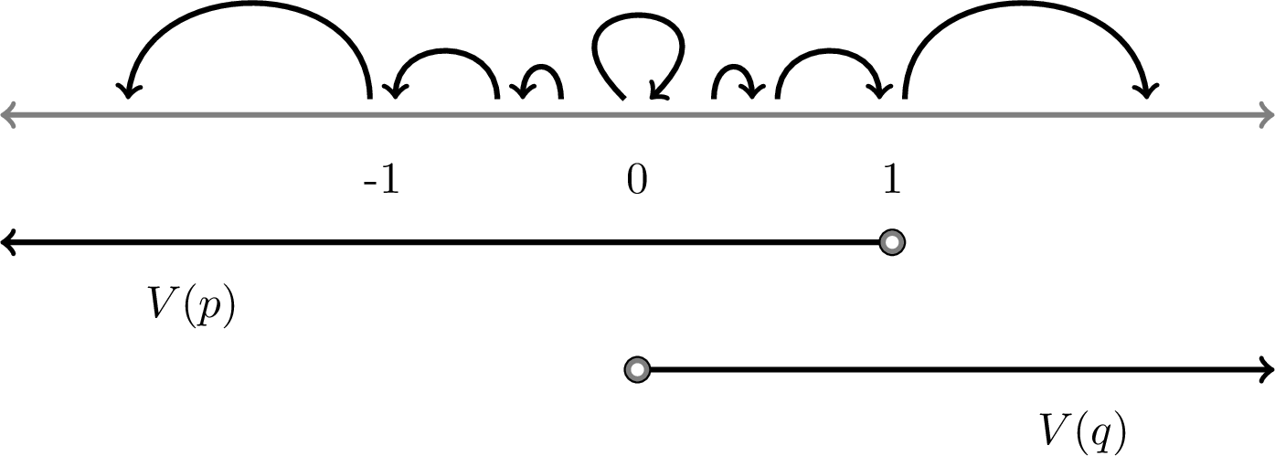
This implies that the proposed axiomatization above cannot be complete for expanding models, as otherwise there would exist a derivation of \(\mathbf{RV}\) and since the axiomatization is sound with respect to topological models, \(\mathbf{RV}\) would be valid over topological models. Instead of extending \(\mathrm{IM_H}\) with different axioms, we present an alternative and perhaps surprising solution. When extending the language of \(\mathsf{iLTL}\) with the co-implication connective \(\mathbin{\tikz[baseline=-.5ex] \draw[-to reversed] (0,0) -- (1em,0);}\), the natural axiomatization becomes ‘magically’ complete. This is because the presence of \(\mathbin{\tikz[baseline=-.5ex] \draw[-to reversed] (0,0) -- (1em,0);}\) and temporal modalities creates implicit interaction, which can be used to derive formulas such as \(\mathbf{RV}\). Thus the derivation of \(\mathbf{RV}\) (see Example 6.3) features formulas with co-implications, even though \(\mathbf{RV}\) itself belongs to the \(\mathbin{\tikz[baseline=-.5ex] \draw[-to reversed] (0,0) -- (1em,0);}\)-free fragment. Thus, our axiomatization is not conservative over the \(\mathbin{\tikz[baseline=-.5ex] \draw[-to reversed] (0,0) -- (1em,0);}\)-free fragment. The resulting logic is called bi-intuitionistic linear temporal logic \(\mathsf{biLTL}\), which contains \(\mathsf{iLTL}\) as a fragment.
The next two sections introduce the syntax and semantics of \(\mathsf{biLTL}\), as well as the axiomatization \(\mathrm{biLTL_H}\). We will then establish soundness as well as completeness for the axiomatization obtained from \(\mathrm{biLTL_H}\) restricted to the language without \(\mathbin{\Box}\) and \(\Diamond\). The final sections then establish completeness for \(\mathrm{biLTL_H}\).
6.2 Syntax and Semantics↩︎
The language of bi-intuitionistic temporal logic \(\mathcal{L}_\mathsf{biLTL}\) extends \(\mathcal{L}_\mathsf{IPL}\) by the temporal operators \(\mathbin{{\bigcirc}}\), \(\Diamond\) and \(\mathbin{\Box}\), as well as by the binary connective \(\mathbin{\tikz[baseline=-.5ex] \draw[-to reversed] (0,0) -- (1em,0);}\). The operators \(\Diamond\) and \(\mathbin{\Box}\) are fixed point operators. \(\Diamond\varphi\) is characterized as the least fixed point of the propositional function \(x \mapsto \varphi \vee \mathbin{{\bigcirc}}x\). \(\mathbin{\Box}\varphi\) is characterized as the greatest fixed point of the propositional function \(x \mapsto \varphi \wedge \mathbin{{\bigcirc}}x\). Formulas are given by the following grammar in Backus–Naur form (where \(p \in \mathsf{Prop}\)): \[\varphi \mathrel{\vcenter{:}}= \bot \mid p \mid \varphi \wedge \varphi \mid \varphi \vee \varphi \mid \varphi \rightarrow \varphi \mid \varphi \mathbin{\tikz[baseline=-.5ex] \draw[-to reversed] (0,0) -- (1em,0);}\varphi \mid \mathbin{{\bigcirc}}\varphi \mid \Diamond\varphi \mid \mathbin{\Box}\varphi\] As before, the connective \(\mathbin{\tikz[baseline=-.5ex] \draw[-to reversed] (0,0) -- (1em,0);}\) is called co-implication and the temporal operators \(\mathbin{{\bigcirc}}\), \(\Diamond\) and \(\mathbin{\Box}\) are read as ‘next’, ‘eventually’ and ‘henceforth’, respectively. The \(\Diamond\)- and \(\mathbin{\Box}\)-free fragment of \(\mathcal{L}_\mathsf{biLTL}\) is denoted by \(\mathcal{L}_{\mathbin{{\bigcirc}}}\). As for bi-intuitionistic modal logic in the previous chapter, the constant \(\bot\) can be defined in terms of \(\mathbin{\tikz[baseline=-.5ex] \draw[-to reversed] (0,0) -- (1em,0);}\) by setting \(\bot \mathrel{\vcenter{:}}= p \mathbin{\tikz[baseline=-.5ex] \draw[-to reversed] (0,0) -- (1em,0);}p\) for \(p \in \mathsf{Prop}\) and we will treat \(\bot\) as a defined constant henceforth. Moreover, we also once again define weak negation \(\sim\) by \({\sim} \varphi \mathrel{\vcenter{:}}= \top \mathbin{\tikz[baseline=-.5ex] \draw[-to reversed] (0,0) -- (1em,0);}\varphi\). Formulas of \(\mathcal{L}_\mathsf{biLTL}\) are evaluated over (total functional) expanding models as used for \(\mathsf{iLTL}\) in Chapter 5. Let us briefly recall the definition.
Definition 6.1. An expanding model* is a total functional dynamic model \({\mathcal{M}=(M, {\leq}, f, V)}\), where \(f\) is forward-confluent.*
Recall that \(f\) being forward confluent is equivalent to \(f\) being order-preserving.
Definition 6.2. Let \({\mathcal{M}=(W, \leq, f, V)}\) be an expanding model. The truth relation* \(\models\) between worlds of \(\mathcal{M}\) and formulas is defined by extending Definition 2.7 with the following clauses, where \(w \in W\).*
| \(\mathcal{M},w \models \varphi \mathbin{\tikz[baseline=-.5ex] \draw[-to reversed] (0,0) -- (1em,0);}\psi\) | iff | \(\exists v \leq w\) : \(\mathcal{M},v \models \varphi\) and \(\mathcal{M},v \not \models \psi\) |
| \(\mathcal{M},w \models \Diamond\varphi\) | iff | there exists \(n < \omega\) : \(\mathcal{M},f^n(w) \models \varphi\) |
| \(\mathcal{M},w \models \mathbin{\Box}\varphi\) | iff | for all \(n < \omega\) : \(\mathcal{M},f^n(w) \models \varphi\) |
A formula \(\varphi\) is satisfiable over the class of expanding models if there exists an expanding model \(\mathcal{M}\) and a world \(w\) with \(\mathcal{M}, w \models \varphi\) and unsatisfiable otherwise. Moreover, \(\varphi\) is valid if \(\mathcal{M}, w \models \varphi\) for all expanding models \(\mathcal{M}\) and all worlds \(w\) and falsifiable otherwise.
Lemma 6.1 (Monotonicity). Let \(\mathcal{M}=(W, {\leq}, f,V)\) be an expanding model, \(w \in W\), and \(\varphi\) be a formula. If \(\mathcal{M},w \models \varphi\) and \(w \leq v\), then \(\mathcal{M},v \models \varphi\).
Proof. By induction on the structure of \(\varphi\). The base cases as well as the cases for \(\varphi = \psi \ast \gamma\) for \(\ast \in \{\wedge, \vee, \rightarrow\}\) are covered in Lemma 3.2. The case for \(\varphi = \psi \mathbin{\tikz[baseline=-.5ex] \draw[-to reversed] (0,0) -- (1em,0);}\gamma\) is covered in Lemma [l: monotonicity for biml] and the cases for \(\varphi = \mathbin{{\bigcirc}}\psi\) and \(\varphi = \Diamond\psi\) are covered in Lemma 5.4 (recall that \(\Diamond\) is definable in terms of \(\mathbin{\mathsf{U}}\)). Suppose \(\varphi = \mathbin{\Box}\psi\) and \(\mathcal{M}, w \models \mathbin{\Box}\psi\). Then for all \(n < \omega\), \(\mathcal{M}, f^n(w) \models \psi\). Since \(w \leq v\), Lemma 5.2 implies that for all \(n < \omega\), \(f^n(w) \leq f^n(v)\). By induction hypothesis \(\mathcal{M}, f^n(v) \models \psi\) for all \(n < \omega\), hence \(\mathcal{M}, v \models \mathbin{\Box}\psi\). ◻
Definition 6.3. The set of valid \(\mathcal{L}_\mathsf{biLTL}\)-formulas over the class of expanding models is denoted by \(\mathbf{biLTL}\).
6.3 Axiomatization↩︎
This section introduces the axiomatization \(\mathrm{biLTL_H}\) that captures \(\mathcal{L}_\mathsf{biLTL}\)-validities over expanding models. As mentioned in the introduction, to obtain a sound and complete system in the presence of co-implication it suffices to expand \(\mathrm{iLTL_H}\) by standard rules for \(\mathbin{\Box}\). This implies that the system \(\mathrm{biLTL_H}\) does not contain any axioms or rules for the interaction between co-implication and the temporal modalities.
Definition 6.4. The Hilbert-style axiomatization \(\mathrm{biLTL_H}\) consists of the axiom schemes and rules depicted in Table ¿tbl:tab:axioms32and32rules32of32biltl?.
| \(\mathsf{biPC}\) | all bi-intuitionistic tautologies |
| \(\mathsf{D}\) | \({\neg} {\X} \bot\) |
| \(\mathsf{Dist}\) | \(\X (\varphi \vee \psi) \to (\X \varphi \vee \X \psi)\) |
| \(\mathsf{K}\) | \(\X (\varphi \rightarrow \psi) \rightarrow (\X \varphi \rightarrow \X \psi)\) |
| \(\mathsf{Fix}_{\E}\) | \((\varphi\vee\X\E \varphi)\to\E \varphi\) |
| \(\mathsf{Fix}_{\G}\) | \(\G\varphi\to (\varphi\wedge{\X}{\G}\varphi)\) |
| \(\mathsf{MP}\) | \(\infer{\psi}{\varphi & \varphi \rightarrow \psi}\) | ||
| \(\mathsf{Nec}\) | \(\infer{\X \varphi}{\varphi}\) | \(\mathsf{DN}\) | \(\infer{\neg{\sim} \varphi}{\varphi }\) |
| \(\mathsf{Mon}_{\E}\) | \(\infer{\E\varphi\to \E\psi }{ \varphi\to\psi}\) | \(\mathsf{Mon}_{\G}\) | \(\infer{\G\varphi\to \G\psi }{ \varphi\to\psi}\) |
| \(\mathsf{Ind}_{\E}\) | \(\infer{\E\varphi\to \varphi }{\X\varphi\to\varphi}\) | \(\mathsf{Ind}_{\G}\) | \(\infer{ \varphi\to \G \varphi }{ \varphi\to\X \varphi}\) |
We also define the Hilbert-style axiomatization \(\mathrm{biLTL_H^{\mathbin{{\bigcirc}}}}\) which is obtained from \(\mathrm{biLTL_H}\) by restricting the language (and therefore the axioms and rules) to \(\mathcal{L}_{\mathbin{{\bigcirc}}}\). For example, a formula \(\varphi\) is an instance of an axiom scheme of \(\mathrm{biLTL_H^{\mathbin{{\bigcirc}}}}\) if \(\varphi \in \mathcal{L}_{\mathbin{{\bigcirc}}}\) and is an instance of an axiom scheme of \(\mathrm{biLTL_H}\).
Definition 6.5. The Hilbert-style axiomatization \(\mathrm{biLTL_H^{\mathbin{{\bigcirc}}}}\) consists of the axioms \(\mathsf{biPC}\), \(\mathsf{D}\), \(\mathsf{Dist}\), \(\mathsf{K}\) and the rules \(\mathsf{MP}\), \(\mathsf{Nec}\) and \(\mathsf{DN}\).
Definition 6.6. Let \(\Gamma \cup \{\varphi\}\) be a set of \(\mathcal{L}_\mathsf{biLTL}\)-formulas or of \(\mathcal{L}_{\mathbin{{\bigcirc}}}\)-formulas, respectively. A derivation with assumptions in \(\Gamma\)* of \(\varphi\) in \(\mathrm{biLTL_H}\) or \(\mathrm{biLTL_H^{\mathbin{{\bigcirc}}}}\) is a finite tree \(\pi\) labelled by \(\mathcal{L}_\mathsf{biLTL}\)-formulas or \(\mathcal{L}_{\mathbin{{\bigcirc}}}\)-formulas, respectively, and according to the rules of \(\mathrm{biLTL_H}\), such that*
every leaf of \(\pi\) is labelled by an axiom or by a formula in \(\Gamma\), and
if a node \(u\) is labelled by the conclusion of a rule instance of a rule different than \(\mathsf{MP}\), then every leaf of the subtree of \(\pi\) rooted at \(u\) is labelled by an axiom.
We write \(\Gamma \vdash \varphi\) if \(\varphi\) has a derivation with assumptions in \(\Gamma\) and \(\vdash \varphi\) if \(\Gamma = \emptyset\). Furthermore, we write \(\Gamma \vdash \Delta\) where \(\Delta\) is any set of formulas if there exists a finite subset \(\Delta_0 \subseteq \Delta\) with \(\Gamma \vdash \bigvee \Delta_0\). Note that every \(\mathrm{biLTL_H^{\mathbin{{\bigcirc}}}}\)-derivation is a \(\mathrm{biLTL_H}\)-derivation. Similarly, every \(\mathrm{biLTL_H}\)-derivation in which only formulas of \(\mathcal{L}_{\mathbin{{\bigcirc}}}\) occur is a \(\mathrm{biLTL_H^{\mathbin{{\bigcirc}}}}\)-derivation. Thus we will not display in the notation \(\Gamma \vdash \varphi\) whether derivability is in \(\mathrm{biLTL_H}\) or \(\mathrm{biLTL_H^{\mathbin{{\bigcirc}}}}\), however, it will always be clear from context. The Deduction Theorem for \(\mathrm{biLTL_H}\) and \(\mathrm{biLTL_H^{\mathbin{{\bigcirc}}}}\) is proven as Theorem 3.3; the proof is omitted.
Theorem 6.1 (Deduction Theorem). Let \(\Gamma\cup \{\varphi, \psi\}\) be a set of \(\mathcal{L}_\mathsf{biLTL}\)- or \(\mathcal{L}_{\mathbin{{\bigcirc}}}\)-formulas. Then \(\Gamma, \varphi \vdash \psi\) if and only if \(\Gamma \vdash \varphi \rightarrow \psi\).
The following lemma is proven in [87].
Lemma 6.2. For arbitrary formulas in \(\mathcal{L}_\mathsf{biLTL}\) the following hold.
\(\vdash \varphi \rightarrow ( \psi \vee \chi) \text{ if and only if } {\vdash (\varphi \mathbin{\tikz[baseline=-.5ex] \draw[-to reversed] (0,0) -- (1em,0);}\psi) \rightarrow \chi }\).
If \(\vdash \varphi\to \varphi'\) and \(\vdash \psi'\to\psi\), then \(\vdash (\varphi\mathbin{\tikz[baseline=-.5ex] \draw[-to reversed] (0,0) -- (1em,0);}\psi) \to(\varphi'\mathbin{\tikz[baseline=-.5ex] \draw[-to reversed] (0,0) -- (1em,0);}\psi')\).
We will now illustrate how (implicit) interaction between co-implication and temporal modalities arise in proofs of our calculus.
Example 6.2.
One might expect that in the presence of co-implication a dual version of the standard \(\mathsf{K}\)-axiom, namely \((\mathbin{{\bigcirc}}\varphi \mathbin{\tikz[baseline=-.5ex] \draw[-to reversed] (0,0) -- (1em,0);}\mathbin{{\bigcirc}}\psi) \rightarrow \mathbin{{\bigcirc}}(\varphi \mathbin{\tikz[baseline=-.5ex] \draw[-to reversed] (0,0) -- (1em,0);}\psi)\) is required in the axiomatization. However, this formula is in fact derivable in \(\mathrm{biLTL_H^{\mathbin{{\bigcirc}}}}\). To see this, observe that the formula \(\varphi\rightarrow (\psi\vee (\varphi\mathbin{\tikz[baseline=-.5ex] \draw[-to reversed] (0,0) -- (1em,0);}\psi))\) is a substitution instance of a bi-intuitionistic tautology and hence derivable. Applying \(\mathsf{Nec}\) yields \[\mathbin{{\bigcirc}}(\varphi\rightarrow (\psi\vee (\varphi\mathbin{\tikz[baseline=-.5ex] \draw[-to reversed] (0,0) -- (1em,0);}\psi))).\] Using axiom \(\mathsf{K}\) and \(\mathsf{MP}\) we obtain \[\mathbin{{\bigcirc}}\varphi \rightarrow \mathbin{{\bigcirc}}(\psi \vee (\varphi \mathbin{\tikz[baseline=-.5ex] \draw[-to reversed] (0,0) -- (1em,0);}\psi))\] Using axiom \(\mathsf{Dist}\) and \(\mathsf{MP}\) yields that \[\mathbin{{\bigcirc}}\varphi\to (\mathbin{{\bigcirc}}\psi\vee \mathbin{{\bigcirc}}(\varphi\mathbin{\tikz[baseline=-.5ex] \draw[-to reversed] (0,0) -- (1em,0);}\psi))\] is derivable. By Lemma 6.2, this shows that \((\mathbin{{\bigcirc}}\varphi\mathbin{\tikz[baseline=-.5ex] \draw[-to reversed] (0,0) -- (1em,0);}\mathbin{{\bigcirc}}\psi )\rightarrow \mathbin{{\bigcirc}}(\varphi\mathbin{\tikz[baseline=-.5ex] \draw[-to reversed] (0,0) -- (1em,0);}\psi)\) is derivable as well.
Example 6.3. The formula \(\mathbf{RV}\), i.e. \(\mathbin{\Box}(\varphi\vee\psi)\rightarrow (\Diamond\varphi\vee\mathbin{\Box}\psi)\), is derivable in \(\mathrm{biLTL_H}\). To see this, note that by Lemma [l: bi-int tautologies] the formula \[\mathbin{\Box}(\varphi\vee\psi)\rightarrow(\Diamond\varphi\vee(\mathbin{\Box}(\varphi\vee\psi)\mathbin{\tikz[baseline=-.5ex] \draw[-to reversed] (0,0) -- (1em,0);}\Diamond\varphi))\] is a substitution instance of a bi-intuitionistic tautology, so it suffices to check that \[\label{e:32example32RV321} (\mathbin{\Box}(\varphi\vee\psi)\mathbin{\tikz[baseline=-.5ex] \draw[-to reversed] (0,0) -- (1em,0);}\Diamond\varphi)\rightarrow \mathbin{\Box}\psi\qquad{(2)}\] is derivable. By \(\mathsf{Fix_{\Diamond/ \mathbin{\Box}}}\), the formulas \(\mathbin{\Box}(\varphi\vee\psi) \rightarrow {\mathbin{{\bigcirc}}\mathbin{\Box}} (\varphi\vee\psi)\) and \(\mathbin{{\bigcirc}}\Diamond\varphi \rightarrow \Diamond\varphi\) are derivable. So Lemma 6.2 implies that \[(\mathbin{\Box}(\varphi\vee\psi)\mathbin{\tikz[baseline=-.5ex] \draw[-to reversed] (0,0) -- (1em,0);}\Diamond\varphi)\rightarrow ({\mathbin{{\bigcirc}}\mathbin{\Box}}(\varphi\vee\psi)\mathbin{\tikz[baseline=-.5ex] \draw[-to reversed] (0,0) -- (1em,0);}\mathbin{{\bigcirc}}\Diamond\varphi))\] is derivable as well. Hence by Example 6.2, \[(\mathbin{\Box}(\varphi\vee\psi)\mathbin{\tikz[baseline=-.5ex] \draw[-to reversed] (0,0) -- (1em,0);}\Diamond\varphi)\to \mathbin{{\bigcirc}}( \mathbin{\Box}(\varphi\vee\psi)\mathbin{\tikz[baseline=-.5ex] \draw[-to reversed] (0,0) -- (1em,0);}\Diamond\varphi)\] is derivable. Using \(\mathsf{Ind}_{\mathbin{\Box}}\) gives that \[(\mathbin{\Box}(\varphi\vee\psi)\mathbin{\tikz[baseline=-.5ex] \draw[-to reversed] (0,0) -- (1em,0);}\Diamond\varphi)\rightarrow \mathbin{\Box}( \mathbin{\Box}(\varphi\vee\psi)\mathbin{\tikz[baseline=-.5ex] \draw[-to reversed] (0,0) -- (1em,0);}\Diamond\varphi)\] is derivable, implying that in order to prove (?? ) it suffices to show that
\[\label{e:32example32RV322} (\mathbin{\Box}(\varphi\vee\psi)\mathbin{\tikz[baseline=-.5ex] \draw[-to reversed] (0,0) -- (1em,0);}\Diamond\varphi)\rightarrow \psi\qquad{(3)}\]
is derivable. Note that \(\mathbin{\Box}(\varphi\vee\psi)\rightarrow \varphi\vee\psi\) and \(\varphi\to\Diamond\varphi\) are derivable by \(\mathsf{Fix_{\mathbin{\Box}}}\) and \(\mathsf{Fix_{\Diamond}}\). Thus we obtain that \[( \mathbin{\Box}(\varphi\vee\psi)\mathbin{\tikz[baseline=-.5ex] \draw[-to reversed] (0,0) -- (1em,0);}\Diamond\varphi) \rightarrow ((\varphi\vee \psi )\mathbin{\tikz[baseline=-.5ex] \draw[-to reversed] (0,0) -- (1em,0);}\varphi)\] is derivable by Lemma 6.2. But \(((\varphi\vee \psi )\mathbin{\tikz[baseline=-.5ex] \draw[-to reversed] (0,0) -- (1em,0);}\varphi) \rightarrow \psi\) is a substitution instance of a bi-intuitionistic tautology; hence \(( \mathbin{\Box}(\varphi\vee\psi)\mathbin{\tikz[baseline=-.5ex] \draw[-to reversed] (0,0) -- (1em,0);}\Diamond\varphi) \rightarrow \psi\) is derivable, as desired.
The rest of this section establishes that \(\mathrm{biLTL_H}\) (and hence also \(\mathrm{biLTL_H^{\mathbin{{\bigcirc}}}}\)) is sound with respect to expanding models.
Lemma 6.3. The axioms of \(\mathrm{biLTL_H}\) are valid over the class of expanding models and the rules preserve validity.
Proof. For the axioms we only check the cases for the modalities. Let \(\mathcal{M}=(W, {\leq}, f,V)\) be an expanding model and \(w \in W\) a world.
Axiom \(\mathsf{D}\). Observe that for any \(v \geq w\) the world \(f(v)\) exists and therefore \(\mathcal{M},v \not \models \mathbin{{\bigcirc}}\bot\). Hence \(\mathcal{M},w \models {\neg} {\mathbin{{\bigcirc}}} {\bot}\).
Axiom \(\mathsf{Dist}\). Let \(v \geq w\) be any world such that \(\mathcal{M},v \models \mathbin{{\bigcirc}}(\varphi \vee \psi)\). Thus \(\mathcal{M}, f(v) \models \varphi \vee \psi\) and so \(\mathcal{M},f(v) \models \varphi\) or \(\mathcal{M},f(v) \models \psi\). Therefore \(\mathcal{M}, v \models \mathbin{{\bigcirc}}\varphi\) or \(\mathcal{M},v \models \mathbin{{\bigcirc}}\psi\) and so \(\mathcal{M},v \models \mathbin{{\bigcirc}}\varphi \vee \mathbin{{\bigcirc}}\psi\). We conclude that \(\mathcal{M},w \models \mathbin{{\bigcirc}}(\varphi \vee \psi) \rightarrow (\mathbin{{\bigcirc}}\varphi \vee \mathbin{{\bigcirc}}\psi)\).
Axiom \(\mathsf{K}\). Let \(v \geq w\) be any world such that \(\mathcal{M},v \models \mathbin{{\bigcirc}}(\varphi \rightarrow \psi)\). Then \(\mathcal{M}, f(v) \models \varphi \rightarrow \psi\). Suppose \(u \geq v\) and \(\mathcal{M},u \models \mathbin{{\bigcirc}}\varphi\). Hence \(\mathcal{M}, f(u) \models \varphi\). By forward confluence, \(f(v) \leq f(u)\) and since \(\mathcal{M},f(v) \models \varphi \rightarrow \psi\), \(\mathcal{M}, f(u) \models \psi\). Thus \(\mathcal{M},u \models \mathbin{{\bigcirc}}\psi\) and so \(\mathcal{M},v \models \mathbin{{\bigcirc}}\varphi \rightarrow \mathbin{{\bigcirc}}\psi\). From this we conclude that \(\mathcal{M},w \models \mathbin{{\bigcirc}}(\varphi \rightarrow \psi) \rightarrow (\mathbin{{\bigcirc}}\varphi \rightarrow \mathbin{{\bigcirc}}\psi)\).
Axiom \(\mathsf{Fix_\Diamond}\). Let \(v \geq w\) be any world such that \(\mathcal{M},v \models \varphi \vee \mathbin{{\bigcirc}}\Diamond\varphi\). Then \(\mathcal{M},v \models \varphi\) or \(\mathcal{M},v \models \mathbin{{\bigcirc}}\Diamond\varphi\). In both cases, \(\mathcal{M},v \models \Diamond\varphi\). Hence \(\mathcal{M},w \models (\varphi \vee \mathbin{{\bigcirc}}\Diamond\varphi) \rightarrow \Diamond\varphi\).
Axiom \(\mathsf{Fix_{\mathbin{\Box}}}\). Let \(v \geq w\) be any world such that \(\mathcal{M},v \models \mathbin{\Box}\varphi\). Then \(\mathcal{M},f^n(v) \models \varphi\) for all \(n < \omega\). In particular, \(\mathcal{M},v \models \varphi\) and \(\mathcal{M},f^n(f(v)) \models \varphi\) for all \(n < \omega\). Thus \(M,f(v) \models \mathbin{\Box}\varphi\) and so \(\mathcal{M},v \models {\mathbin{{\bigcirc}}} {\mathbin{\Box}} \varphi\). Together, \(\mathcal{M},v \models \varphi \wedge {\mathbin{{\bigcirc}}} {\mathbin{\Box}} \varphi\), and so \(\mathcal{M},w \models {\mathbin{\Box}} \varphi \rightarrow \varphi \wedge {\mathbin{{\bigcirc}}} {\mathbin{\Box}} \varphi\).
For the rules we check all cases with the exception of \(\mathsf{MP}\) and \(\mathsf{Nec}\).
Rule \(\mathsf{DN}\). Suppose that \(\varphi\) is valid. Let \(v\) be any world such that \(v \geq w\). Let \(u\) be any world such that \(u \leq v\). Since \(\varphi\) is valid, \(\mathcal{M},u \models \varphi\). As \(u\) is an arbitrary world, we conclude that \(\mathcal{M},v \not \models {\sim} \varphi\). As \(v\) is an arbitrary world as well, it follows that \(\mathcal{M},w \models {\neg} {\sim} \varphi\). Hence \({\neg} {\sim} \varphi\) is valid.
Rule \(\mathsf{Mon}_\Diamond\). Suppose \(\varphi \rightarrow \psi\) is valid. Let \(v \geq w\) be any world and suppose \(\mathcal{M},v \models \Diamond\varphi\). So there exists \(n < \omega\) such that \(\mathcal{M},f^n(v) \models \varphi\). Since \(\mathcal{M},f^n(v) \models \varphi \rightarrow \psi\), also \(\mathcal{M},f^n(v) \models \psi\). Hence, \(\mathcal{M},v \models \Diamond\psi\), and so \(\mathcal{M},w \models \Diamond\varphi \rightarrow \Diamond\psi\). We conclude that \(\Diamond\varphi \rightarrow \Diamond\psi\) is valid.
Rule \(\mathsf{Mon}_{\mathbin{\Box}}\). Suppose \(\varphi \rightarrow \psi\) is valid. Let \(v \geq w\) be any world and suppose that \(\mathcal{M},v \models \mathbin{\Box}\varphi\). So for all \(n < \omega\) it holds that \(\mathcal{M},f^n(v) \models \varphi\). Since for each \(n < \omega\), \(\mathcal{M}, f^n(v) \models \varphi \rightarrow \psi\), it also holds that \(\mathcal{M},f^n(v) \models \psi\). Thus \(\mathcal{M},v \models \mathbin{\Box}\psi\), and so \(\mathcal{M},w \models \mathbin{\Box}\varphi \rightarrow \mathbin{\Box}\psi\). We conclude that \(\mathbin{\Box}\varphi \rightarrow \mathbin{\Box}\psi\) is valid.
Rule \(\mathsf{Ind}_\Diamond\). Suppose \(\mathbin{{\bigcirc}}\varphi \rightarrow \varphi\) is valid. We first show that for any \(n < \omega\), \(\mathcal{M},f^n(w) \models \varphi\) implies \(\mathcal{M},w \models \varphi\) by induction on \(n\). The base case where \(n=0\) is trivial. For the induction step suppose that the claim holds for \(n=k\) and consider the case where \(n=k+1\). If \(\mathcal{M},f^{k+1}(w) \models \varphi\), then \(\mathcal{M},f^k(w) \models \mathbin{{\bigcirc}}\varphi\). Since \(\mathbin{{\bigcirc}}\varphi \rightarrow \varphi\) is valid, we have \(\mathcal{M},f^k(w) \models \varphi\). By the induction hypothesis, \(\mathcal{M},w \models \varphi\), which concludes the proof of the claim. Next, let \(v \geq w\) be any world and suppose \(\mathcal{M},v \models \Diamond\varphi\). Then there exists \(n < \omega\) with \(\mathcal{M},f^n(v) \models \varphi\). By the previous claim it follows that \(\mathcal{M},v \models \varphi\). Hence \(\mathcal{M},w \models \Diamond\varphi \rightarrow \varphi\), and so \(\Diamond\varphi \rightarrow \varphi\) is valid.
Rule \(\mathsf{Ind}_{\mathbin{\Box}}\). Suppose \(\varphi \rightarrow \mathbin{{\bigcirc}}\varphi\) is valid. We first show that \(\mathcal{M},w \models \varphi\) implies \(\mathcal{M},f^n(w) \models \varphi\) for all \(n < \omega\) by induction on \(n\). The base case where \(n=0\) is trivial. For the induction step suppose the claim holds for \(n=k\) and consider the case for \(n=k+1\). By the induction hypothesis \(\mathcal{M},f^k(w) \models \varphi\). Since \(\varphi \rightarrow \mathbin{{\bigcirc}}\varphi\) is valid, \(\mathcal{M},f^k(w) \models \mathbin{{\bigcirc}}\varphi\), and therefore \(\mathcal{M},f^{k+1}(w) \models \varphi\), which concludes the proof of the claim. Next, let \(v \geq w\) be any world such that \(\mathcal{M},v \models \varphi\). By the previous claim it follows that \(\mathcal{M},f^n(v) \models \varphi\) for all \(n < \omega\), and thereby that \(\mathcal{M},v \models \mathbin{\Box}\varphi\). Thus \(\mathcal{M},w \models \varphi \rightarrow \mathbin{\Box}\varphi\), implying that \(\varphi \rightarrow \mathbin{\Box}\varphi\) is valid. ◻
From the previous lemma, soundness of \(\mathrm{biLTL_H}\) is inferred by a standard induction on the height of proofs.
Theorem 6.2 (Soundness of \(\mathrm{biLTL_H}\)). For any \(\mathcal{L}_\mathsf{biLTL}\)-formula \(\varphi\) if \(\varphi\) is provable in \(\mathrm{biLTL_H}\), then \(\varphi\) is valid over the class of expanding models.
6.4 Completeness for the Next-Fragment↩︎
This section establishes completeness of \(\mathrm{biLTL_H^{\mathbin{{\bigcirc}}}}\) by emplyoing a standard canonical model construction. As the canonical model is also used later on in the completeness proof of \(\mathrm{biLTL_H}\), the following definitions and lemmas apply to both \(\mathcal{L}_\mathsf{biLTL}\) and \(\mathcal{L}_{\mathbin{{\bigcirc}}}\). Write \(\mathcal{L}\) for \({\mathcal{L} \in \{ \mathcal{L}_\mathsf{biLTL},\mathcal{L}_{\mathbin{{\bigcirc}}}\}}\).
Definition 6.7. An \(\mathcal{L}\)-prime theory* is a set of \(\mathcal{L}\)-formulas \(\Gamma\), such that the following hold.*
\(\Gamma\) is deductively closed: if \(\Gamma \vdash \varphi\), then \(\varphi \in \Gamma\).
\(\Gamma\) satisfies the disjunction property: if \(\varphi \vee \psi \in \Gamma\), then \(\varphi \in \Gamma\) or \(\psi \in \Gamma\).
\(\Gamma\) is consistent: \(\Gamma \not \vdash \bot\).
The following properties are readily checked for any prime theory \(\Gamma\) (see Lemma 3.16).
Lemma 6.4. Let \(\Gamma\) be a \(\mathcal{L}\)-prime theory and \(\varphi, \psi \in \mathcal{L}\).
\(\varphi \wedge \psi \in \Gamma\) if and only if \(\varphi \in \Gamma\) and \(\psi \in \Gamma\).
\(\varphi \vee \psi \in \Gamma\) if and only if \(\varphi \in \Gamma\) or \(\psi \in \Gamma\).
If \(\varphi \rightarrow \psi \in \Gamma\), then \(\varphi \not \in \Gamma\) or \(\psi \in \Gamma\).
If \(\varphi \mathbin{\tikz[baseline=-.5ex] \draw[-to reversed] (0,0) -- (1em,0);}\psi \in \Gamma\), then \(\varphi \in \Gamma\).
If \(\Diamond\varphi \in \Gamma\), then \(\varphi \in \Gamma\) or \({\mathbin{{\bigcirc}}}{\Diamond}\varphi \in \Gamma\).
If \(\mathbin{\Box}\varphi \in \Gamma\), then \(\varphi \in \Gamma\) and \({\mathbin{{\bigcirc}}}{\mathbin{\Box}}\varphi \in \Gamma\).
Given a set of formulas \(\Gamma\), define \(\mathbin{{\bigcirc}}^{-1} \Gamma \mathrel{\vcenter{:}}= \{\varphi \mid \mathbin{{\bigcirc}}\varphi \in \Gamma\}\).
Lemma 6.5. If \(\Gamma\) is a prime theory, then \(\mathbin{{\bigcirc}}^{-1}\Gamma\) is a prime theory as well.
Proof. Suppose \(\Gamma\) is a prime theory. We check all three properties of a prime theory.
1. Suppose \(\mathbin{{\bigcirc}}^{-1}\Gamma \vdash \varphi\) by derivation \(\pi\), where \(\pi\) is a \(\mathrm{biLTL_H}\)- or a \(\mathrm{biLTL_H^{\mathbin{{\bigcirc}}}}\)-derivation. We proceed by induction on the height of \(\pi\). In the base case \(\varphi\) is an axiom or belongs to \(\mathbin{{\bigcirc}}^{-1} \Gamma\). If \(\varphi\) is an axiom, then by necessitation, \(\Gamma \vdash \mathbin{{\bigcirc}}\varphi\) and therefore by the fact that \(\Gamma\) is deductively closed \(\mathbin{{\bigcirc}}\varphi \in \Gamma\). Hence \(\varphi \in \mathbin{{\bigcirc}}^{-1} \Gamma\). If instead \(\varphi\) belongs to \(\mathbin{{\bigcirc}}^{-1} \Gamma\), then there is nothing left to show. For the induction step first suppose the last rule applied in \(\pi\) is \(\mathsf{MP}\) with conclusion \(\varphi\) and premises \(\psi\) and \(\psi \rightarrow \varphi\). By induction hypothesis \(\psi, \psi \rightarrow \varphi \in \mathbin{{\bigcirc}}^{-1} \Gamma\). Hence \(\mathbin{{\bigcirc}}\psi, \mathbin{{\bigcirc}}(\psi \rightarrow \varphi) \in \Gamma\). By the presence of the \(\mathsf{K}\)-axiom and \(\mathsf{MP}\) we conclude that \(\mathbin{{\bigcirc}}\varphi \in \Gamma\), and thus \(\varphi \in \mathbin{{\bigcirc}}^{-1} \Gamma\). Next, suppose the last rule applied in \(\pi\) is \(\mathsf{R}\) where \(\mathsf{R} \not = \mathsf{MP}\), with premise \(\psi\) and conclusion \(\gamma\). By definition of a derivation from assumptions it must hold that \(\psi\) is provable from the empty set, i.e. \(\vdash \psi\), and hence \(\vdash \gamma\) as well. Thus applying \(\mathsf{Nec}\) yields \(\vdash \mathbin{{\bigcirc}}\gamma\), and so \(\Gamma \vdash \mathbin{{\bigcirc}}\gamma\). Since \(\Gamma\) is deductively closed, \(\mathbin{{\bigcirc}}\gamma \in \Gamma\), implying that \(\gamma \in \mathbin{{\bigcirc}}^{-1} \Gamma\).
2. Suppose \(\varphi \vee \psi \in \mathbin{{\bigcirc}}^{-1} \Gamma\). Then \(\mathbin{{\bigcirc}}(\varphi \vee \psi) \in \Gamma\). By \(\mathsf{Dist}\) and \(\mathsf{MP}\), \(\mathbin{{\bigcirc}}\varphi \vee \mathbin{{\bigcirc}}\psi \in \Gamma\). As \(\Gamma\) satisfies the disjunction property, \(\mathbin{{\bigcirc}}\varphi \in \Gamma\) or \(\mathbin{{\bigcirc}}\psi \in \Gamma\). Hence \(\varphi \in \mathbin{{\bigcirc}}^{-1} \Gamma\) or \(\psi \in \mathbin{{\bigcirc}}^{-1} \Gamma\).
3. Suppose towards contradiction that \(\mathbin{{\bigcirc}}^{-1} \Gamma \vdash \bot\). Then \(\bot \in \mathbin{{\bigcirc}}^{-1} \Gamma\) as \(\mathbin{{\bigcirc}}^{-1} \Gamma\) is deductively closed. Thus \(\mathbin{{\bigcirc}}\bot \in \Gamma\). But \(\Gamma \vdash {\neg} {\mathbin{{\bigcirc}}} \bot\), and thus \(\Gamma \vdash \bot\); a contradiction. ◻
Next, the standard Lindenbaum Lemma holds for \(\mathrm{biLTL_H}\) and \(\mathrm{biLTL_H^{\mathbin{{\bigcirc}}}}\). The proof is from [87].
Lemma 6.6 (Lindenbaum). Let \(\Gamma \cup \{\gamma\} \subseteq \mathcal{L}\). If \(\Gamma \not \vdash \gamma\), then there exists a \(\mathcal{L}\)-prime theory \(\Delta\) with \(\Gamma \subseteq \Delta\) and \(\Delta \not \vdash \gamma\).
Proof. Suppose \(\Gamma \not \vdash \gamma\) and consider an arbitrary enumeration of the formulas of \(\mathcal{L}\). We first show how to construct a set of formulas \(\Delta_n\) for each \(n < \omega\) by induction on \(n\).
Define \(\Delta_0 \mathrel{\vcenter{:}}= \Gamma\)
Suppose we have defined \(\Delta_n\). Let \(\varphi \vee \psi\) be the first formula in the enumeration that has a disjunction as its principal connective, has not yet been treated in a previous step and \(\Delta_n \vdash \varphi \vee \psi\). Then define \(\Delta_{n+1}\) as follows:
\[\Delta_{n+1} \mathrel{\vcenter{:}}= \begin{cases} \Delta_n \cup \{\varphi\} \text{ if } \Delta_n, \varphi \not \vdash \gamma\\ \Delta_n \cup \{\psi\} \text{ otherwise. }\\ \end{cases}\]
Observe that for each \(n < \omega\) holds that \(\Delta_n \subseteq \Delta_{n+1}\). Define \(\Delta\) to be \[\Delta \mathrel{\vcenter{:}}= \bigcup_{n < \omega} \Delta_n\] By construction \(\Gamma \subseteq \Delta\). In order to show that \(\Delta\) is a prime theory, let us first check whether it satisfies the disjunction property. If \(\varphi \vee \psi \in \Delta\), then \(\Delta \vdash \varphi \vee \psi\). Let \(n\) be the least natural number such that \(\Delta_n \vdash \varphi \vee \psi\). By construction there exists \(m \geq n\) such that either \(\varphi\) or \(\psi\) is added to \(\Delta_{m+1}\). Thus, since \(\Delta_{m+1} \subseteq \Delta\) it holds that \(\varphi \in \Delta\) or \(\psi \in \Delta\). In order to show that \(\Delta\) is deductively closed, suppose that \(\Delta \vdash \varphi\). Then \(\Delta \vdash \varphi \vee \varphi\), and thus \(\varphi \in \Delta\) by the same argument as above. In order to show that \(\Delta \not \vdash \gamma\), we first prove by induction on \(n\) that each \(\Delta_n \not \vdash \gamma\). The base case holds by assumption. So suppose that \(\Delta_n \not \vdash \gamma\) and the formula treated at that step is \(\varphi \vee \psi\). If \(\Delta_{n+1} = \Delta_n \cup \{\varphi\}\), then \(\Delta_{n+1} \not \vdash \gamma\) by construction. Otherwise \(\Delta_n \cup \{\varphi\} \vdash \gamma\) and \(\Delta_{n+1} = \Delta_n \cup \{\psi\}\). Suppose towards contradiction that \(\Delta_{n+1} \vdash \gamma\). Therefore \[\begin{align} \Delta_n, \varphi \vdash \gamma\\ \Delta_n, \psi \vdash \gamma\\ \end{align}\] By the Deduction Theorem \(\Delta_n \vdash \varphi \rightarrow \gamma\) and \(\Delta_n \vdash \psi \rightarrow \gamma\). Therefore \(\Delta_n \vdash (\varphi \vee \psi) \rightarrow \gamma\). Since \(\Delta_n \vdash \varphi \vee \psi\) by assumption it therefore follows that \(\Delta_n \vdash \gamma\), a contradiction. Hence \(\Delta_{n+1} \not \vdash \gamma\). Finally if \(\Delta \vdash \gamma\), then \(\Delta_n \vdash \gamma\) for some \(n\). As this cannot be the case, we conclude that \(\Delta \not \vdash \gamma\). Observe that this also implies that \(\Delta\) is consistent and hence a prime theory. ◻
We are now ready to define the canonical models for \(\mathcal{L}_\mathsf{biLTL}\) and \(\mathcal{L}_{\mathbin{{\bigcirc}}}\).
Definition 6.8. Let \(\mathcal{L}\) be either \(\mathcal{L}_{\mathbin{{\bigcirc}}}\) or \(\mathcal{L}_\mathsf{biLTL}\). The canonical model* for \(\mathcal{L}\) is defined to be \(\mathcal{M}_\mathrm{c}=(W_\mathrm{c}, {\leq_\mathrm{c}}, f_\mathrm{c}, V_\mathrm{c})\) where*
\(W_\mathrm{c} = \{ \Gamma \subseteq \mathcal{L} \mid \Gamma\) is a \(\mathcal{L}\)-prime theory\(\}\),
\(\Gamma \leq_\mathrm{c} \Gamma'\) \(\iff\) \(\Gamma \subseteq \Gamma'\),
\(f_\mathrm{c}(\Gamma) = \mathbin{{\bigcirc}}^{-1} \Gamma\),
\(V_\mathrm{c}(\Gamma) = \{ p \in \mathsf{Prop}\mid p \in \Gamma\}\).
Lemma 6.7. The canonical model for either \(\mathcal{L}_{\mathbin{{\bigcirc}}}\) or \(\mathcal{L}_\mathsf{biLTL}\) is an expanding model.
Proof. By definition of \(\leq_c\) holds that \((W_c, \leq_c)\) is a poset and \(V_c\) is monotone. Note that for each \(\Gamma, \Gamma' \in W_c\) if \(\mathbin{{\bigcirc}}^{-1} \Gamma = \mathbin{{\bigcirc}}^{-1} \Gamma'\), then \(\Gamma = \Gamma'\). Moreover by Lemma 6.5, \(\mathbin{{\bigcirc}}^{-1} \Gamma \in W_c\), implying that \(f_c: W_c \longrightarrow W_c\) is well-defined. If \(\Gamma \leq_c \Gamma'\), then \(\Gamma \subseteq \Gamma'\) and so \(\mathbin{{\bigcirc}}^{-1} \Gamma \subseteq \mathbin{{\bigcirc}}^{-1} \Gamma'\), implying that \(f_c (\Gamma) \leq_c f_c (\Gamma')\). Therefore \(\mathcal{M}_c\) is an expanding model. ◻
The proof of the first part of the following lemma is standard, while the second part was proven in [87].
Lemma 6.8 (Witnessing Lemma). Let \(\mathcal{L}\) be either \(\mathcal{L}_{\mathbin{{\bigcirc}}}\) or \(\mathcal{L}_\mathsf{biLTL}\). Let \(\Gamma\) be a \(\mathcal{L}\)-prime theory and \(\psi, \gamma\) any \(\mathcal{L}\)-formulas. The following hold.
\(\psi \rightarrow \gamma \not \in \Gamma\) if and only if there exists a prime theory \(\Delta\) with \(\Gamma \leq_c \Delta\) and \(\psi \in \Delta\) and \(\gamma \not \in \Delta\).
\(\psi \mathbin{\tikz[baseline=-.5ex] \draw[-to reversed] (0,0) -- (1em,0);}\gamma \in \Gamma\) if and only if there exists a prime theory \(\Delta\) with \(\Delta \leq_c \Gamma\) and \(\psi \in \Delta\) and \(\gamma \not \in \Delta\).
Proof. For 1. suppose that \(\psi \rightarrow \gamma \not \in \Gamma\). So \(\Gamma \not \vdash \psi \rightarrow \gamma\). The Deduction Theorem implies that \(\Gamma, \psi \not \vdash \gamma\). By the Lindenbaum Lemma there exists a prime theory \(\Delta\) such that \(\Gamma \cup \{\psi\} \subseteq \Delta\) and \(\gamma \not \in \Delta\). Note that \(\Gamma \leq_c \Delta\). For the other direction suppose \(\psi \rightarrow \gamma \in \Gamma\). Let \(\Delta\) be any prime theory with \(\Gamma \leq_c \Delta\). Then \(\psi \rightarrow \gamma \in \Delta\) and so by Lemma 6.4, \(\psi \not \in \Delta\) or \(\gamma \in \Delta\).
For 2. suppose that \(\psi \mathbin{\tikz[baseline=-.5ex] \draw[-to reversed] (0,0) -- (1em,0);}\gamma \in \Gamma\). Suppose towards contradiction that \(\psi \vdash \gamma, \Gamma^c\) where \(\Gamma^c = \mathcal{L} \setminus \Gamma\). Hence there exists a finite \(\Omega \subseteq \Gamma^c\) such that \(\psi \vdash \gamma \vee \bigvee \Omega\) and so by the Deduction Theorem \[\vdash \psi \rightarrow (\gamma \vee \bigvee \Omega)\] Lemma 6.2 then implies that \[\vdash (\psi \mathbin{\tikz[baseline=-.5ex] \draw[-to reversed] (0,0) -- (1em,0);}\gamma) \rightarrow \bigvee \Omega\] So also \(\Gamma \vdash (\psi \mathbin{\tikz[baseline=-.5ex] \draw[-to reversed] (0,0) -- (1em,0);}\gamma) \rightarrow \bigvee \Omega\). But as \(\psi \mathbin{\tikz[baseline=-.5ex] \draw[-to reversed] (0,0) -- (1em,0);}\gamma \in \Gamma\) we conclude that \[\Gamma \vdash \bigvee \Omega,\] which implies that there exists \(\delta \in \Omega\) such that \(\delta \in \Gamma\) as \(\Gamma\) is prime, contradicting \(\Gamma \cap \Gamma^c = \emptyset\). Therefore \(\psi \not \vdash \gamma,\Gamma^c\). By the Lindenbaum Lemma there exists a prime theory \(\Delta\) such that \(\psi \in \Delta\) and \((\Gamma^c \cup \{\gamma\}) \cap \Delta = \emptyset\). Therefore \(\Delta \subseteq \Gamma\), implying \(\Delta \leq_\mathrm{c} \Gamma\). Finally, observe that by construction \(\psi \in \Delta\) and \(\gamma \not \in \Delta\).
For the other direction suppose that \(\psi \mathbin{\tikz[baseline=-.5ex] \draw[-to reversed] (0,0) -- (1em,0);}\gamma \not \in \Gamma\). So \(\Gamma \not \vdash \psi \mathbin{\tikz[baseline=-.5ex] \draw[-to reversed] (0,0) -- (1em,0);}\gamma\). Moreover, for each \(\Delta \subseteq \Gamma\) it holds that \(\Delta \not \vdash \psi \mathbin{\tikz[baseline=-.5ex] \draw[-to reversed] (0,0) -- (1em,0);}\gamma\). Observe that \[\vdash \psi \rightarrow (\gamma \vee (\psi \mathbin{\tikz[baseline=-.5ex] \draw[-to reversed] (0,0) -- (1em,0);}\gamma)).\] Therefore for every \(\Delta \subseteq \Gamma\) if \(\Delta \vdash \psi\), then \(\Delta \vdash \gamma\) i.e. if \(\psi \in \Delta\), then \(\gamma \in \Delta\). ◻
For the remainder of this section we work exclusively in the language \(\mathcal{L}_{\mathbin{{\bigcirc}}}\) and show that \(\mathrm{biLTL_H^{\mathbin{{\bigcirc}}}}\) is complete.
Lemma 6.9 (Truth Lemma). Let \(\mathcal{M}_\mathrm{c}\) be the canonical model for \(\mathcal{L}_{\mathbin{{\bigcirc}}}\). For every \(\Gamma \in W_\mathrm{c}\) and any \(\mathcal{L}_{\mathbin{{\bigcirc}}}\)-formula \(\varphi\), it holds that
\(\varphi \in \Gamma \text{ if and only if } \mathcal{M}_\mathrm{c}, \Gamma \models \varphi\).
Proof. We proceed by induction on the structure of \(\varphi\). The base case follows immediately from the definition of the valuation \(V_\mathrm{c}\) and the fact that prime theories are consistent. For the induction step the cases where \(\varphi = \psi \wedge \chi\) and \(\varphi = \psi \vee \chi\) are standard and omitted. The cases for \(\varphi= \psi \rightarrow \chi\) and \(\varphi = \psi \mathbin{\tikz[baseline=-.5ex] \draw[-to reversed] (0,0) -- (1em,0);}\chi\) follow immediately from Lemma 6.8 and the induction hypothesis.
\(\varphi = \mathbin{{\bigcirc}}\psi\): For the direction from left to right suppose that \(\mathbin{{\bigcirc}}\psi \in \Gamma\). Then, by definition, \(\psi \in \mathbin{{\bigcirc}}^{-1} \Gamma\). By the induction hypothesis \(\mathcal{M}_\mathrm{c}, \mathbin{{\bigcirc}}^{-1} \Gamma \models \psi\). As \(f_\mathrm{c}(\Gamma) = \mathbin{{\bigcirc}}^{-1} \Gamma\) we conclude that \(\mathcal{M}_\mathrm{c}, \Gamma \models \mathbin{{\bigcirc}}\psi\). For the direction from right to left suppose that \(\mathcal{M}_\mathrm{c}, \Gamma \models \mathbin{{\bigcirc}}\psi\). This implies that \(\mathcal{M}_\mathrm{c},f_\mathrm{c}(\Gamma) \models \psi\). By construction \(f_\mathrm{c}(\Gamma) = \mathbin{{\bigcirc}}^{-1} \Gamma\). By the induction hypothesis \(\psi \in \mathbin{{\bigcirc}}^{-1} \Gamma\). Hence by definition \(\mathbin{{\bigcirc}}\psi \in \Gamma\). ◻
Theorem 6.3 (Completeness of \(\mathrm{biLTL_H^{\mathbin{{\bigcirc}}}}\)). If a \(\mathcal{L}_{\mathbin{{\bigcirc}}}\)-formula \(\varphi\) is valid over the class of expanding models, then \(\varphi\) is \(\mathrm{biLTL_H^{\mathbin{{\bigcirc}}}}\)-derivable.
Proof. Suppose \(\varphi\) is not \(\mathrm{biLTL_H^{\mathbin{{\bigcirc}}}}\)-derivable, i.e. \(\emptyset \not \vdash \varphi\). By the Lindenbaum Lemma there exists a prime theory \(\Gamma\) with \(\Gamma \not \vdash \varphi\). Hence \(\varphi \not \in \Gamma\), and so by the Truth Lemma, \(\mathcal{M}_\mathrm{c}, \Gamma \not \models \varphi\). Therefore \(\varphi\) is not valid. ◻
6.5 Proof Strategy for the Full Language↩︎
The remainder of this chapter is devoted to prove that \(\mathrm{biLTL_H}\) is complete for the class of expanding models. Unlike for \(\mathrm{biLTL_H^{\mathbin{{\bigcirc}}}}\), the Truth Lemma for the canonical model does not hold, since it may be for example that \(\Diamond\varphi\in \Gamma\), but there is no \(n\) such that \(\varphi\in f^n_\mathrm{c}(\Gamma)\). This is because \(\Diamond\varphi \vdash \bigvee _{i<n} \mathbin{{\bigcirc}}^i \varphi\) is not derivable for any specific \(n\), and derivations are finite. Hence it is possible for \(\Diamond\varphi\) to hold but each individual \(\mathbin{{\bigcirc}}^n \varphi\) to fail in a prime theory.
A similar situation occurs for classical linear temporal logic (\(\mathsf{LTL}\)), but one can then pass to a filtration \(\frac{\mathcal{M}_\mathrm{c}}{\Sigma}\) of \(\mathcal{M}_\mathrm{c}\), i.e. the quotient of \(\mathcal{M}_\mathrm{c}\) modulo the equivalence relation given by \[\Gamma\sim\Gamma' \text{ if and only if } \Gamma\cap \Sigma=\Gamma'\cap \Sigma.\] Assuming \(\Sigma\) is finite, the equivalence class of each prime theory \(\Gamma\) is determined by its characteristic formula \(\chi(\Gamma)\mathrel{\vcenter{:}}= \bigwedge ( \Gamma\cap \Sigma)\).21 The filtrated model does respect the semantics of \(\Diamond\). More precisely, \(\frac{\mathcal{M}_\mathrm{c}}{\Sigma}\) satisfies a version of the Truth Lemma restricted to formulas of \(\Sigma\), which is sufficient as long as \(\Sigma\) contains enough formulas. The tradeoff is that \(\frac{\mathcal{M}_\mathrm{c}}{\Sigma}\) is no longer equipped with a function, as the quotient may assign more than one temporal successor to each equivalence class of prime theories. To see why, recall that if \(\Gamma \sim \Gamma'\), then \(\Gamma \cap \Sigma = \Gamma' \cap \Sigma\). Since \(\Sigma\) is a finite set, it is possible that there exists a formula \(\varphi \in \Sigma\) such that \(\mathbin{{\bigcirc}}\varphi \not \in \Sigma\), and therefore that \(\mathbin{{\bigcirc}}\varphi \in \Gamma\) but \(\mathbin{{\bigcirc}}\varphi \not \in \Gamma'\). This implies that \(f_c(\Gamma) \not \sim f_c(\Gamma')\). Accordingly, the quotient model must relate the equivalence class of \(\Gamma\) with both equivalences of \(f_c(\Gamma)\) and of \(f_c(\Gamma')\).
However, this is not a problem, since in a later phase one can choose a path \(\Gamma_0,\Gamma_1,\Gamma_2,\dots\) that constitutes a genuine \(\mathsf{LTL}\)-model. In particular, if \(\varphi\) is not derivable, we can choose \(\Sigma\) to be the set of subformulas of \(\varphi\) and their negations and \(\Gamma_0\) so that \(\varphi\not\in \Gamma_0\), thereby obtaining a model falsifying \(\varphi\).
We wish to adapt this strategy, but there is an issue: filtration in general does not conserve order-preservation of the temporal dynamics (i.e. \(w \leq v\) implies \(f(w) \leq f(v)\)), so we must define \(\frac{\mathcal{M}_\mathrm{c}}{\Sigma}\) differently. This structure should be a quasimodel, which is similar to a model except that the temporal transition function is replaced by a non-deterministic relation. Each point in a quasimodel is assigned a type, which is similar to a prime theory except that a type only decides a finite set of formulas; i.e., a type is a pair \(\Phi=(\Phi^+,\Phi^-)\) of (usually) finite sets of formulas for which a ‘Truth Lemma’ should hold. In other words, a quasimodel is essentially what was called a labelled model in Chapter [c: bi-int ml new]. Quasimodels are designed so that they can be ‘unwound’ into a genuine model, much like for the filtrated model of classical \(\mathsf{LTL}\).
To construct \(\frac{\mathcal{M}_\mathrm{c}}{\Sigma}\) in the bi-intuitionistic setting, we use the tools and results from Chapter [c: bi-int ml new], where a finite labelled model \(\mathrm I_{ \Sigma }\) was constructed and related to any given model via a dynamic and strongly surjective simulation \(\check{E}_0\). The structure \(\mathrm I_{ \Sigma }\upharpoonright_{dom(\check{E}_0)}\) was shown to be a labelled model, and will play the role of \(\frac{\mathcal{M}_\mathrm{c}}{\Sigma}\) here. These results were given in a general modal setting, however we will show how they can be readily applied to the specific case of \(\mathsf{biLTL}\).
Much as the characteristic formula \(\chi(\Gamma)\) determines the equivalence class of \(\Gamma\) in the classical setting, we can characterise which points of \(\mathrm I_{ \Sigma }\) are \(\check{E}_0\)-related to a given prime theory \(\Gamma\) using simulation formulas. Unlike the classical setting, we need two distinct formulas, \(\chi^+\) and \(\chi^-\), to capture respectively the ‘positive’ and ‘negative’ information determining a simulation. These simulation formulas enable us to prove that \(\frac{\mathcal{M}_\mathrm{c}}{\Sigma}\) is indeed a quasimodel.
At the end of the chapter we put all the ingredients together to show that \(\mathrm{biLTL_H}\) is complete for the class of expanding models: the argument is that if \(\varphi\) is not derivable then we can find a prime theory \(\Gamma\) with \(\varphi\in \Gamma ^-\). By choosing a point \(w\) of \(\frac{\mathcal{M}_\mathrm{c}}{\Sigma}\) with \(w\mathrel {\check{E}_0} \Gamma\), we see that \(\varphi\) is falsified on \(\frac{\mathcal{M}_\mathrm{c}}{\Sigma}\). By applying the unwinding procedure to \(\frac{\mathcal{M}_\mathrm{c}}{\Sigma}\), we obtain a genuine model falsifying \(\varphi\). Thus every formula that is not derivable can be falsified in some expanding model, implying that \(\mathrm{biLTL_H}\) is complete.
6.6 Types, Labelled Structures and Quasimodels↩︎
This section introduces the aforementioned relational structures called quasimodels. Many definitions are akin to the definitions of labelled models in Chapter [c: bi-int ml new], but adjusted to the case of \(\mathsf{biLTL}\). From now on, \(\Sigma\) denotes a set of \(\mathcal{L}_\mathsf{biLTL}\)-formulas closed under subformulas.
Definition 6.9. Let \(\Phi^+, \Phi^- \subseteq \Sigma\). A \(\Sigma\)-type* is a pair \(\Phi = (\Phi^+, \Phi^-)\) of disjoint subsets of \(\Sigma\) satisfying the properties 2. – 7. of Definition [d: type] and the following properties.*
If \(\mathbin{\Box}\varphi \in \Phi^+\), then \(\varphi \in \Phi^+\).
If \(\Diamond\varphi \in \Phi^-\), then \(\varphi \in \Phi^-\).
As before, it is not necessary that \(\Phi^+ \cup \Phi^- = \Sigma\). Thus types are once again ‘partial’. The set of all \(\Sigma\)-types is denoted by \(\mathrm{T}_\Sigma\). The partial orders \(\leq_{\mathrm{T}}\) and \(\subseteq_\mathrm{T}\) are defined as before. Moreover, the notion of a defect of a type is also defined as before, c.f. Definition [d: defects].
Recall the definition of a \(\Sigma\)-labelled poset \(\mathcal{X}=(X, \leq_{\mathcal{X}}, \ell_{\mathcal{X}})\) (c.f. Definition [d: labelled poset]). In Chapter [c: bi-int ml new] sensible relations were defined with respect to a sensibility condition to have a general argument for the multiple frame conditions considered. Here, we only consider one class of frames and therefore only require one specific sensibility condition.
Definition 6.10. Let \(\Phi, \Psi\) be \(\Sigma\)-types. The pair \((\Phi, \Psi)\) is called sensible* if the following conditions hold.*
If \(\mathbin{{\bigcirc}}\varphi \in \Phi^+\), then \(\varphi \in \Psi^+\).
If \(\mathbin{{\bigcirc}}\varphi \in \Phi^-\), then \(\varphi \in \Psi^-\).
If \(\Diamond\varphi \in \Phi^+\), then \(\varphi \in \Phi^+\) or \(\Diamond\varphi \in \Psi^+\).
If \(\Diamond\varphi \in \Phi^-\), then \(\varphi \in \Phi^-\) and \(\Diamond\varphi \in \Psi^-\).
If \(\mathbin{\Box}\varphi \in \Phi^+\), then \(\varphi \in \Phi^+\) and \(\mathbin{\Box}\varphi \in \Psi^+\).
If \(\mathbin{\Box}\varphi \in \Phi^-\), then \(\varphi \in \Phi^-\) or \(\mathbin{\Box}\varphi \in \Psi^-\).
Given a \(\Sigma\)-labelled poset \(\mathcal{X}=(X, {\leq}, \ell)\), a pair \((x,y) \in X \times X\) is called sensible* if \((\ell(x), \ell(y))\) is sensible. A relation \(R \subseteq X \times X\) is called sensible if \(R\) is forth-up and forth-down confluence (with respect to \((\leq_{\mathcal{X}}, \leq_{\mathcal{X}})\)) and every pair \((x,y) \in R\) is sensible.*
One can easily check that the relation \(S \subseteq \mathrm{T}_\Sigma \times \mathrm{T}_\Sigma\) given by
\((\Phi, \Psi) \in S\) if and only if \((\Phi, \Psi)\) is sensible
is a sensibility condition. Therefore every sensible structure considered henceforth is \(S\)-sensible.
Definition 6.11. Given a \(\Sigma\)-labelled poset \(\mathcal{X}=(X, {\leq}, \ell)\), a sensible relation \(R \subseteq X \times X\) is called \(\omega\)-sensible* if the following hold.*
If \(\Diamond\varphi \in \ell(x)^+\), then there are \(n < \omega\) and \(y \in X\) such that \(x \mathrel R^n y\) and \(\varphi \in \ell(y)^+\).
If \(\mathbin{\Box}\varphi \in \ell(x)^-\), then there are \(n < \omega\) and \(y \in X\) such that \(x \mathrel R^n y\) and \(\varphi \in \ell(y)^-\).
Definition 6.12. A \(\Sigma\)-labelled system* is a tuple \(\mathcal{X}=(X, {\leq}, \ell, R)\) consisting of a labelled poset equipped with a sensible relation \(R \subseteq X \times X\). If moreover \(R\) is serial and \(\omega\)-sensible, then \(\mathcal{X}\) is a \(\Sigma\)-quasimodel.*
We may write simply labelled system or quasimodel when \(\Sigma\) is clear from context. A formula \(\varphi\) is falsified at world \(x\) of a \(\Sigma\)-labelled system \(\mathcal{X}=(X, {\leq}, \ell, R)\) if \(\varphi \in \ell(x)^-\), and satisfied if \(\varphi \in \ell(x)^+\). A formula \(\varphi\) is falsifiable over the class of \(\Sigma\)-quasimodels if there exists a \(\Sigma\)-quasimodel \(\mathcal{X}=(X, {\leq}, \ell, R)\) and a world \(x \in X\) such that \(\varphi\) is falsified at \(x\).
Observe that every expanding model can be regarded as a \(\Sigma\)-quasimodel by simply labelling each world with those formulas in \(\Sigma\) that are true or false respectively. Thus we obtain the following result.
Lemma 6.10. If \(\varphi \in \Sigma\) is falsifiable over the class of expanding models, then \(\varphi\) is falsifiable over the class of \(\Sigma\)-quasimodels.
The converse of Lemma 6.10 is also true, but establishing it requires some work. This will be done in the next section. However, we can already state the result for a particular subclass of quasimodels.
Definition 6.13. A \(\Sigma\)-quasimodel \(\mathcal{X}=(X, {\leq}, \ell, R)\) is total functional* if \(R \subseteq X \times X\) is a function.*
Lemma 6.11. If a formula is falsifiable over the class of total functional \(\Sigma\)-quasimodels, then it is falsifiable over the class of expanding models.
Proof. Given a total functional \(\Sigma\)-quasimodel \(\mathcal{X}=(X, {\leq}, \ell, f)\) define an expanding model \(\mathcal{M}=(X, {\leq}, V, f)\) where \(V(y) \mathrel{\vcenter{:}}= \ell(y)^+ \cap \mathsf{Prop}\). Observe that \(\mathcal{M}\) is well-defined. We prove simultaneously that for \(\varphi \in \Sigma\) if \(\varphi \in \ell(x)^+\), then \(\mathcal{M}, x \models \varphi\) and if \(\varphi \in \ell(x)^-\), then \(\mathcal{ M}, x \not \models \varphi\) by induction on \(\varphi\). The base case where \(\varphi \in \mathsf{Prop}\) follows directly from the definition of the valuation. The cases for \(\varphi = \psi \ast \gamma\) for \(\ast \in \{\wedge, \vee, \rightarrow, \mathbin{\tikz[baseline=-.5ex] \draw[-to reversed] (0,0) -- (1em,0);}\}\) follow from the definition of a type and a labelled poset. For example if \(\psi \wedge \gamma \in \ell(x)^-\), then \(\psi \in \ell(x)^-\) or \(\gamma \in \ell(x)^-\). By induction hypothesis \(\mathcal{M}, x \not \models \psi\) or \(\mathcal{M}, x \not \models \gamma\). Thus \(\mathcal{M}, x \not \models \psi \wedge \gamma\). Suppose \(\varphi = \mathbin{{\bigcirc}}\psi \in \ell(x)^-\). By sensibility of \(f\), \(\psi \in \ell(f(x))^-\) and so by induction hypothesis \(\mathcal{M}, f(x) \not \models \psi\). Therefore \(\mathcal{M}, x \not \models \mathbin{{\bigcirc}}\psi\). The case for \(\mathbin{{\bigcirc}}\psi \in \ell(x)^+\) is similar. Suppose \(\varphi = \Diamond\psi \in \ell(x)^-\). By definition of a type \(\psi \in \ell(x)^-\) and \(\Diamond\psi \in \ell(f(x))^-\). By a simple induction on \(n\) it follows that \(\psi, \Diamond\psi \in \ell(f^n(x))^-\) for all natural numbers \(n\). Thus by induction hypothesis \(\mathcal{M}, f^n(x) \not \models \psi\) for all \(n\), implying that \(\mathcal{M},x \not \models \Diamond\psi\). Suppose \(\Diamond\psi \in \ell(x)^+\). Then by \(\omega\)-sensibility there exists a natural number \(n\) such that \(\psi \in \ell(f^n(x))\). By induction hypothesis \(\mathcal{M}, f^n(x) \models \psi\) and therefore \(\mathcal{M}, x \models \Diamond\psi\). The cases for \(\varphi = \mathbin{\Box}\psi\) are similar. ◻
6.7 From Quasimodels to Expanding Models↩︎
This section establishes that if a formula in \(\mathcal{L}_\mathsf{biLTL}\) is falsifiable over the class of quasimodels, then it is falsifiable over the class of expanding models. Given a quasimodel falsifying a formula \(\varphi\), we will show how to construct a total functional quasimodel which falsifies \(\varphi\) as well. The construction is similar to the construction of a functional model from a dynamic model presented in Chapter 3, Section 3.3, however the confluence conditions complicate the argument. Applying Lemma 6.11 then yields an expanding model which falsifies \(\varphi\). For the construction it is useful to observe that forward confluence can be iterated, thereby yielding the following lemma for finite \(R\)-paths, which is a generalization of Lemma 5.2.
Lemma 6.12. Let \(\mathcal{X}=(X, {\leq}, \ell, R)\) be a quasimodel and \(w_0, \ldots w_n \in X\) such that \(w_0\mathrel R w_1 \mathrel R \dots \mathrel R w_n\).
If \(w_0\leq u_0\), then there exist \(u_0\mathrel R u_1 \mathrel R \dots \mathrel R u_n\) such that \(w_i\leq u_i\) for all \(i\leq n\).
If \(u_0\leq w_0\) then there exist \(u_0\mathrel R u_1 \mathrel R \ldots \mathrel R u_n\) such that \(u_i\leq w_i\) for all \(i\leq n\).
Proof. For 1. proceed by induction on the length \(n\) of the path \(w_0, \ldots, w_n\). For \(n=0\) the statement is vacuously true. For \(n> 0\) there exist \(u_0 \mathrel R u_1 \mathrel R \ldots \mathrel R u_{n-1}\) with \(w_i \leq u_i\) for all \(i < n\) by induction hypothesis. In particular, \(w_{n-1} \leq u_{n-1}\). Since \(w_{n-1} \mathrel R w_n\), forth-up confluence yields \(u_n \in X\) with \(u_{n-1} \mathrel R u_n\) and \(w_n \leq u_n\). The same argument using forth-down confluence instead of forth-up confluence suffices to also show 2. ◻
For the remainder of this section let \(\mathcal{X}=(X, {\leq}, \ell, R)\) be a fixed \(\Sigma\)-quasimodel. Suppose that \(\mathcal{X}\) falsifies some formula \(\varphi \in \Sigma\). We are now going to show how to construct from \(\mathcal{X}\) a total functional \(\Sigma\)-quasimodel falsifying \(\varphi\). Recall that \(\exists{f(x)}\) denotes that \(x \in dom(f)\) and \(\nexists{f(x)}\) that \(x \not \in dom(f)\) for \(f\) a partial function.
Definition 6.14. An \(\mathcal{X}\)-induced structure* is a tuple \(\mathcal{I} =(I, {\leq_I}, \ell_I, f_I)\) together with a map \(\pi\colon I\to X\) where:*
\(I\) is finite,
\(\leq_I\) is acyclic and if \(w \leq_I v\) then \(\pi(w)\leq \pi(v)\),
\(\ell_I = \ell_X \circ \pi\), and
\(f_I: I \to I\) is a partial function such that:
If \(\exists{f_I(x)}\), then \(\pi(x) \mathrel R \pi ( f_I(x))\).
If \(x \leq_I y\) then \(\exists{f(x)} \iff \exists{f(y)}\).
If \(x \leq_I y\) and \(\exists{f(x)}\), then \(f_I(x) \leq_I f_I(y)\).
For each \(x\in I\) there is a maximal \(k\) such that \(\exists{f^k(x)}\).
In view of [maximal] and the assumption that \(I\) is finite, there is a maximal \(k\) such that \(f^k(x)\) is defined for any \(x\in I\), and hence we may define \(W_{i}\) to be the set of \(x\in I\) such that \(f^{k-i}(x)\) is defined but \(f^{k-i+1}(x)\) is not. This partitions \(I\) into sets \(W_0,\ldots,W_k\), and it is easy to see that \(x \leq_I y\) implies that \(x,y\in W_i\) for some \(i\), and moreover \(f[W_i]\subseteq W_{i+1}\) for all \(i\).
A defect of an \(\mathcal{X}\)-induced structure records that a claim made by its labelling \(\ell_I\) lacks a witness.
Definition 6.15. Let \(\mathcal{I}\) be an \(\mathcal{X}\)-induced structure.
A \(\rightarrow\)-defect* is a pair \((x, \varphi \rightarrow \psi)\) where \(x \in I\) and \(\varphi \rightarrow \psi \in \ell_I(x)^-\), but there is no \(y \geq_I x\) with \(\varphi \in \ell_I(y)^+\) and \(\psi \in \ell_I(y)^-\).*
A \(\mathbin{\tikz[baseline=-.5ex] \draw[-to reversed] (0,0) -- (1em,0);}\)-defect is a pair \((x, \varphi \mathbin{\tikz[baseline=-.5ex] \draw[-to reversed] (0,0) -- (1em,0);}\psi)\) where \(x \in I\) and \(\varphi \mathbin{\tikz[baseline=-.5ex] \draw[-to reversed] (0,0) -- (1em,0);}\psi \in \ell_I(x)^+\), but there is no \(y \leq_I x\) with \(\varphi \in \ell_I(y)^+\) and \(\psi \in \ell_I(y)^-\).
A \(\mathbin{{\bigcirc}}\)-defect* is a world \(x \in I\) with \(\nexists{f_I(x)}\).*
A \(\Diamond\)-defect* is a pair \((x, \Diamond\varphi)\) where \(x \in I\), \(\nexists{f_I(x)}\), and \(\Diamond\varphi \in \ell_I(x)^+\), but \(\varphi \not \in \ell_I(x)^+\).*
A \(\mathbin{\Box}\)-defect* is a pair \((x, \mathbin{\Box}\varphi)\) where \(x \in I\), \(\nexists{f_I(x)}\), and \(\mathbin{\Box}\varphi \in \ell_I(x)^-\), but \(\varphi \not \in \ell_I(x)^-\).*
Let \(x \in X\) be such that \(\varphi \in \ell(x)^-\). We build a total functional \(\Sigma\)-quasimodel falsifying \(\varphi\) in stages. We start with an \(\mathcal{X}\)-induced structure \(\mathcal{I}_0\) consisting of a single world and then construct in the step \(n+1\) an \(\mathcal{X}\)-induced structure \(\mathcal{I}_{n+1}\) extending \(\mathcal{I}_n\). We make use of a first-in-first-out queue \(D\) that stores the defects of the current \(\mathcal{X}\)-induced structure. Observe that for any \(\mathcal{X}\)-induced structure, the set of defects of said structure is always finite (since the structure and \(\Sigma\) are finite) and non-empty (due to \(\mathbin{{\bigcirc}}\)-defects). The \(\mathcal{X}\)-induced structure \(\mathcal{I}_n\) is defined by induction on \(n\) as follows.
Base case: Define \(\mathcal{I}_0=(I_0, {\leq_0}, \ell_0, f_0)\), where \(I_0 = \{x'\}\) (where \(x'\) is a fresh world not occurring in \(X\)), \({\leq_0} = \{(x',x')\}\), \(\ell_0(x') = \ell(x)\), \(f_0 = \emptyset\), and \(\pi_0(x') = x\). It is straightforward to check that \((\mathcal{I}_0, \pi_0)\) is an \(\mathcal{X}\)-induced structure. Initialise \(D\) with all defects of \(\mathcal{I}_0\) in arbitrary order.
Induction step: Suppose we have defined \(\mathcal{I}_{n}=(I_n, {\leq_n}, \ell_n, f_n)\) and \(\pi_n\), and shown that \((\mathcal{I}_{n},\pi_{n})\) is an \(\mathcal{X}\)-induced structure. By induction hypothesis, \(D\) currently stores all defects of \(\mathcal{I}_n\). We first show how to define \((\mathcal{I}_{n+1},\pi_{n+1})\) and then how to update the queue \(D\). We start by setting \(I_{n+1} = I_n\) and proceed by a case distinction on the defect at the head of the queue \(D\).
(\(\mathbin{{\bigcirc}}\)-defects) Suppose the defect at the head of \(D\) is a \(\mathbin{{\bigcirc}}\)-defect \(y \in I_n\). Choose any \(u \in X\) with \(\pi_n(y)\mathrel R u\). Add a new point \(u'\) to \(I_{n+1}\) and define \(f_{n+1}(y)= u'\), \(\ell_{n+1}(u') = \ell(u)\), and \(\pi_{n+1}(u')=u\). We extend \(f_{n+1}\) to the connected component of \(y\) by adding new worlds, working first ‘bottom up’ starting with worlds covering \(y\). If \(y'\) covers \(y\), use forth-up confluence to find \(z \in X\) with \(\pi_n(y')\mathrel R z\). Add a fresh node \(z'\) to \(\mathcal{I}_{n+1}\) and define \(f_{n+1}(y') = z'\), \(u' \leq_{n+1} z'\) and close \(\leq_{n+1}\) under transitivity and reflexivity,22, \(\pi_{n+1}(z')= z\), and \(\ell_{n+1}(z')=\ell(z)\). Then for \(y''\) covering such \(y'\), use forth-up confluence again (relative to \(y'\)) to define \(f_{n+1}(y'')\), and so on. Next repeat the process for those worlds below \(\{y' \mid y' \geq y\}\) where \(f_{n+1}\) is not yet defined, this time working ‘top down’ and using forth-down confluence. Continue alternating between ‘bottom up’ and ‘top down’ until \(f_{n+1}\) is defined on the connected component of \(y\).
This process terminates because the newly added points are not in the connected component of \(y\), which is finite. Thus if the connected component of \(y\) in \(\mathcal{I}_n\) is of size \(m\), then \(m\) new points are added.
(\(\rightarrow\)-defects) Suppose the defect at the head of \(D\) is a \(\rightarrow\)-defect \((y, \psi \rightarrow \chi)\). Then \(\psi \rightarrow \chi \in \ell_n(y)^-\), but there is no \(z' \in I_n\) with \(y \leq_n z'\), and \(\varphi \in \ell_n(z')^+\) and \(\psi \in \ell_n(z')^-\). As \(\mathcal{X}\) is a quasimodel, there exists \(\pi_n(y) \leq z \in X\) with \(\psi \in \ell(z)^+\) and \(\chi \in \ell(z)^-\). Let \(k\) be largest natural number such that \(f^k_n(y)\) is defined. Using Lemma 6.12, find \(z=z_0\mathrel R z_1\mathrel R\dots \mathrel R z_k\) with \(\pi_n(f^i_n(y)) \leq z_i\). Then add fresh points \(z'_0,\ldots,z'_k\) to \(I_{n+1}\) and extend \(\pi_n\), \(\leq_n\), \(f_n\) and \(\ell_n\) by setting \(\pi_{n+1}(z'_i)=z_i\), \(f^i_n(y) \leq_{n+1} z'_i\), \(f_{n+1}(z'_i)=z'_{i+1}\) and \(\ell_{n+1}(z'_i)=\ell(z_i)\).
This process terminates because there is a maximal number \(l\) such that every point in \(I_n\) has at most \(l\) temporal successors. Therefore \(k \leq l\) new points are added.
(\(\mathbin{\tikz[baseline=-.5ex] \draw[-to reversed] (0,0) -- (1em,0);}\)-defects) Suppose the defect at the head of \(D\) is a \(\mathbin{\tikz[baseline=-.5ex] \draw[-to reversed] (0,0) -- (1em,0);}\)-defect \((y, \psi \mathbin{\tikz[baseline=-.5ex] \draw[-to reversed] (0,0) -- (1em,0);}\chi)\). The construction of \((\mathcal{I}_{n+1}, \pi_{n+1})\) is then just as for \(\rightarrow\)-defects.
(\(\Diamond\)-defects) Suppose the defect at the head of \(D\) is a \(\Diamond\)-defect \((y, \Diamond\psi)\). Then \(\nexists{f_n(y)}\) and \(\Diamond\psi \in \ell_n(y)^+\), but \(\psi \not \in \ell_n(y)^+\). As \(\mathcal{X}\) is a quasimodel we find \(u_1, \ldots, u_n \in X\) with \(\pi_n(y)\mathrel R u_1\mathrel R u_2\mathrel R \ldots\mathrel R u_n\) and \(\psi \in \ell(u_n)^+\). We add worlds \(u'_1, \ldots, u'_n\) to \(I_{n+1}\) with \(\pi_{n+1}(u'_i) = u_i\), \(f_{n+1}(y) = u'_{1}\) and \(f_{n+1}(u'_i) = u'_{i+1}\), and \(\ell_{n+1}(u'_i) = \ell (u_i)\). Then we proceed as in the case of a \(\mathbin{{\bigcirc}}\)-defect to define \(f_{n+1}\) on the connected component of \(y\), and proceed inductively to define \(f_{n+1}\) on the connected component of each \(u'_i\). In this case, we must add \(n\)-many components for some natural number \(n\). Hence, the construction for ‘next’-defects must be repeated \(n\)-many times. Thus the termination of this process is proven by induction on \(n\), with a secondary induction on the number of worlds in a component as in the \(\mathbin{{\bigcirc}}\)-defect case.
(\(\mathbin{\Box}\)-defects) Suppose the defect at the head of \(D\) is a \(\mathbin{\Box}\)-defect \((y, \mathbin{\Box}\psi)\). The construction is then as for \(\Diamond\)-defects.
Updating D We have shown how to construct \((\mathcal{I}_{n+1}, \pi_{n+1})\) from \((\mathcal{I}_n, \pi_n)\). Next we show how to update the queue \(D\). First, delete every defect from \(D\) that has been resolved in the construction of \((\mathcal{I}_{n+1}, \pi_{n+1})\) (observe that in each of the above cases it is possible that multiple defects have been resolved at once). Then each remaining defect is rewritten as follows. Remaining \(\rightarrow\)- or \(\mathbin{\tikz[baseline=-.5ex] \draw[-to reversed] (0,0) -- (1em,0);}\)-defects are left unchanged. For an \(\Diamond\)-defect \((y, \Diamond\psi)\) if \(\nexists{f_{n+1}(y)}\) holds, then the defect is left unchanged. Otherwise there are \(u_1, \ldots, u_k\) with \(f_{n+1}(y)=u_1, f_{n+1}(u_1)=u_2, \ldots, f_{n+1}(u_{k-1}) = u_k\) and \(\nexists{f_{n+1}(u_k)}\). By assumption \(\Diamond\psi \in \ell_{n+1}(u_k)^+\) and \(\psi \not \in \ell_{n+1}(u_k)^+\). Thus overwrite \((y, \Diamond\psi)\) with \((u_k, \Diamond\psi)\). The \(\mathbin{\Box}\)-defects and \(\mathbin{{\bigcirc}}\)-defects are overwritten in the same way. Finally, add all new defects of \(\mathcal{I}_{n+1}\) to the tail of the queue.
Lemma 6.13. For each \(n < \omega\), \(\mathcal{I}_n\) is an \(\mathcal{X}\)-induced structure.
Proof. Proceed by induction on \(n\). For the base case it is easily checked that \(\mathcal{I}_0\) is an \(\mathcal{X}\)-induced structure. Suppose \(\mathcal{I}_n\) is an \(\mathcal{X}\)-induced structure and consider \(\mathcal{I}_{n+1}\). As shown in the construction above, \(\mathcal{I}_{n+1}\) is obtained from \(\mathcal{I}_n\) by resolving a defect of \(\mathcal{I}_n\). Furthermore it was shown that for each defect only finitely many new points were added. Therefore \(I_{n+1}\) is finite. That \(\leq_{n+1}\) is acyclic follows from \(\leq_n\) being acyclic and the fact that whenever a new point \(x'\) is added above or below an existing point \(x\), then \(x'\) is only related (via \(\leq_{n+1}\)) to \(x\) (and every point reachable via transitivity and reflexivity) but unrelated to any other point in \(I_n\). For example, if \(\mathcal{I}_{n+1}\) is obtained from resolving an implication defect \((x, \varphi \rightarrow \psi)\), it is possible that the construction finds \(z \geq \pi_n(x)\) and there exists \(y \geq_n x\) with \(\pi(y) \geq z\). In that case, the construction does not add a new point \(x'\) to \(I_n\) with \(x \leq_{n+1} x' \leq_{n+1} y\), but instead adds a fresh copy \(x'\) to \(I_n\) with \(x' \geq_{n+1} x\) and \(x'\) unrelated to \(y\). This ensures that no cycles are created in the construction for each defect. If \(x \leq_{n+1} y\), then either \(x \leq_n y\) or (without loss of generality) \(y\) was added in the construction to generate \(\mathcal{I}_{n+1}\). In the first case \(\pi_{n+1}(x) \leq \pi_{n+1}(y)\). In the second case, the construction for each defect guarantees that \(\pi_{n+1}(x) \leq \pi_{n+1}(y)\). That \(\ell_{n+1}(x) = \ell(\pi(x))\) follows directly from the induction hypothesis (in case \(x \in I_n\)) and from the construction otherwise. For 4. each item follows directly from the construction. ◻
Observe that by construction, each \(\mathcal{I}_{n+1}\) contains \(\mathcal{I}_n\) as a substructure. Define \((\mathcal{I}_\omega \mathrel{\vcenter{:}}= (I_\omega, {\leq_\omega}, \ell_\omega, f_\omega), \pi_\omega)\) where \[\lambda_\omega = \bigcup_{n < \omega} \lambda_n\] for \(\lambda \in \{I, {\leq}, \ell, f, \pi\}\). Observe that \(x' \in I_\omega\) with \(\pi_\omega(x') = x\) and therefore \(\varphi \in \ell_\omega(x')^-\). Thus \(\mathcal{I}_\omega\) falsifies \(\varphi\).
Lemma 6.14. The structure \((I_\omega, \leq_\omega, \ell_\omega)\) is a \(\Sigma\)-labelled poset.
Proof. That \((I_\omega, \leq_\omega)\) is a partial order follows from the fact that \(\leq_\omega\) is an increasing union of partial orders. The labelling function \(\ell_\omega\) satisfies the property that for each \(y \in I_\omega\), \(\ell_\omega(y) = \ell(\pi_\omega(y))\). Hence \(\ell_\omega\) assigns \(\Sigma\)-types to worlds in \(I_\omega\) and so \((I_\omega, \leq_\omega, \ell_\omega)\) is \(\Sigma\)-labelled. Suppose \(y \leq_\omega z\). Then \(\pi_\omega(y) \leq \pi_\omega(z)\), and thus \(\ell(\pi_\omega(y)) \leq_{\mathrm{T}} \ell(\pi_\omega(z))\). From the previous observation, it follows that \(\ell_\omega(y) \leq_{\mathrm{T}} \ell_\omega(z)\). Suppose \(y \in I_\omega\) and \(\psi \rightarrow \chi \in \delta \ell_\omega(y)\). So \(\psi \rightarrow \chi \in \ell_\omega(y)^-\) but \(\psi \not \in \ell_\omega(y)^+\). Let \(n\) be the least natural number such that \(y \in I_n\). First suppose that there exists a world \(z \in I_n\) with \(y \leq_n z\) and \(\psi \in \ell_n(z)^+\) and \(\chi \in \ell_n(z)^-\). Then \(z \in I_\omega\) and since \(\ell_n (z) = \ell_\omega(z)\) we are done. Otherwise at the end of step \(n\) the queue \(D\) is updated and the defect \((y, \psi \rightarrow \chi)\) is added to \(D\). Then there exists \(k \geq n\) such that at step \(k\) the defect \((y, \psi \rightarrow \chi)\) is resolved (either the defect is at the head of \(D\) and is resolved actively or another defect is resolved that also resolves \((y, \psi \rightarrow \chi)\)). Thus in \(\mathcal{I}_{k+1}\) there exists a world \(z \geq_{k+1} y\) with \(\psi \in \ell_n(z)^+\) and \(\chi \in \ell_n(z)^-\). By construction \(z \in I_\omega\). The case for co-implication defects is analogous. ◻
Lemma 6.15. \(f_\omega\) is a total function.
Proof. By construction \(f_\omega \subseteq I_\omega \times I_\omega\). We check that \(f_\omega\) is total and functional. For totality, let \(y \in I_\omega\), and let \(n\) be the least natural number for which \(y \in I_n\). Then either \(\exists{f_n(y)}\) or at step \(n\) \(y\) is added to \(D\) as a \(\mathbin{{\bigcirc}}\)-defect. In that case there exists \(m \geq n\) at which \(y\) is resolved, implying that \(\exists{f_m(y)}\). Both cases imply that \(\exists{f_\omega(y)}\). For functionality if \(f_n(y) = z\), let us call \(z\) a ‘temporal successor of \(y\)’. It then suffices to observe—by inspection of the construction and property 4(b) of an \(\mathcal{X}\)-induced structure—that the construction adds for each world at most one temporal successor. ◻
Combining these results we obtain the following lemma.
Lemma 6.16. \(\mathcal{I}_\omega\) is a functional \(\Sigma\)-quasimodel falsifying \(\varphi\).
Proof. That \((I_\omega, \leq_\omega, \ell_\omega)\) is a \(\Sigma\)-labelled poset is Lemma 6.14. That \(f_\omega : I_\omega \to I_\omega\) is a total function is Lemma 6.15. For forth–up and forth–down confluence observe that \(f_\omega\) satisfies both of these confluence properties if and only if \(f_\omega\) is order-preserving, due to the fact that \(f_\omega\) is a function (c.f. Lemma 2.7). Thus suppose that \(y \leq_\omega z\). Let \(n\) be the least natural number for which \(y,z \in I_n\) and \(\exists{f_n(y)}\) and \(\exists{f_n(z)}\). Observe that \(y \leq_n z\). Since \(\mathcal{I}_n\) is an \(\mathcal{X}\)-induced structure, Property 4(c) of such a structure guarantees that \(f_n(y) \leq_n f_n(z)\). Hence \(f_\omega(y) \leq_\omega f_\omega(z)\), i.e. \(f_\omega\) is order-preserving. Next, for any \(y \in I_\omega\) by construction \(\pi_\omega(y)\mathrel R \pi_\omega(f_\omega(y))\), and so \(f_\omega\) is sensible. Next, suppose that for \(y \in I_\omega\) and \(\Diamond\psi \in \Sigma\) it holds that \(\Diamond\psi \in \ell_\omega(y)^+\). If \(\psi \in \ell_\omega(y)^+\), then we are done. Otherwise let \(n\) be the least natural number for which \(y \in I_n\). Since \(\ell_n(y) = \ell_\omega(y)\) we have that \(\Diamond\psi \in \ell_n(y)^+\) and \(\psi \not \in \ell_n(y)^+\). Suppose \(f_n^k(y) = y_k\) and \(\nexists{f_n(y_k)}\). Then either there exists \(1 \leq i \leq k\) with \(\psi \in \ell_n(f_n^i(y))^+\) or \((y_k, \Diamond\psi)\) is added to the queue \(D\) as a \(\Diamond\)-defect. In the first case \(\psi \in \ell_\omega(f_\omega^i(y))^+\). In the second case let \(l\) be the natural number bigger \(n\) such that in the \(l\)-th step the defect \((y_k, \Diamond\psi)\) (or its corresponding defect obtained from rewriting \((y_k, \Diamond\psi)\) finitely many times) is deleted from \(D\). Thus \(\mathcal{I}_l\) contains a world \(u\) such that \(f_l^j(y) = u\) for some \(j \geq 1\) and \(\psi \in \ell_l(u)^+\). Hence there exists \(j < \omega\) with \(\psi \in \ell_\omega(f_\omega^j(y))^+\). The case for \(\mathbin{\Box}\psi\) is similar and therefore \(f_\omega\) is \(\omega\)-sensible. Finally, by construction, \(x' \in I_\omega\) and \(\varphi \in \ell_\omega(x')^-\). Putting everything together, \(\mathcal{I}_\omega\) is a functional \(\Sigma\)-quasimodel falsifying \(\varphi\). ◻
Finally, we obtain the main result of this section:
Theorem 6.4. A formula \(\varphi\) is falsifiable over the class of expanding models if and only if \(\varphi\) is falsifiable over the class of \(\Sigma\)-quasimodels.
Proof. The left-to-right direction is Lemma 6.10. For the right-to-left direction, suppose \(\varphi\) is falsifiable over the class of \(\Sigma\)-quasimodels. Hence there exists a \(\Sigma\)-quasimodel \(\mathcal{X}=(X, {\leq}, \ell, R)\) and \(x \in X\) with \(\varphi \in \ell(x)^-\). By Lemma 6.16 there exists a functional \(\Sigma\)-quasimodel falsifying \(\varphi\). So by Lemma 6.11 there exists an expanding model falsifying \(\varphi\). Thus \(\varphi\) is falsifiable over the class of expanding models. ◻
6.8 Simulations↩︎
A key ingredient in our completeness proof will be to relate worlds in a finite quasimodel to prime theories in the canonical model. As in chapter [c: bi-int ml new] dynamic simulations will be used to achieve this. Let us briefly recall the definitions.
Definition 6.16. Let \(\Sigma \subseteq \Delta \subseteq \mathcal{L}_\mathsf{biLTL}\) be subformula closed, and let \(\mathcal{X} = (X, {\leq_\mathcal{X}}, \ell_\mathcal{X})\) and \(\mathcal{Y} = (Y, {\leq_\mathcal{Y}}, \ell_\mathcal{Y})\) be \(\Sigma\)-labelled and \(\Delta\)-labelled posets respectively. A binary relation \(E \subseteq X \times Y\) is a simulation* if the following hold:*
If \(x \mathrel E y\), then \(\ell_\mathcal{X}(x) \subseteq_\mathrm{T} \ell_\mathcal{Y}(y)\).
\(E\) is forth-up and forth-down confluence with respect to \((\leq_\mathcal{X}, \leq_\mathcal{Y})\).
If there exists a simulation \(E\) such that \(x \mathrel E y\), then we write \((\mathcal{X},x) \rightharpoonup (\mathcal{Y},y)\).
The following result is crucial for the completeness argument, yet straighforward to prove. Given labelled systems \(\mathcal{X}=(X, \leq_\mathcal{X}, \ell_\mathcal{X}, R_\mathcal{X})\) and \(\mathcal{Y}=(Y, \leq_\mathcal{Y}, \ell_\mathcal{Y}, R_\mathcal{Y})\) and a simulation \(E \subseteq X \times Y\), let \(X{\upharpoonright_{dom(E)}}\) be the structure obtained from restricting \(\mathcal{X}\) to the domain of \(E\), as before.
Lemma 6.17. Let \(\mathcal{X}\), \(\mathcal{Y}\) be labelled systems and \(E \subseteq X\times Y\) a simulation. Then \(\mathcal{X}{\upharpoonright_{dom(E)}}\) is a labelled system.
Proof. Denote \(\mathcal{X}{\upharpoonright_{dom(E)}}\) by \(\mathcal{Z}=(Z, \leq_\mathcal{Z}, \ell_\mathcal{Z}, R_\mathcal{Z})\) where \(Z = dom (E)\). That \((Z, \leq_\mathcal{Z})\) is a poset follows directly from \((X, \leq_\mathcal{X})\) being a poset and \((Z, \leq_\mathcal{Z})\) being the restriction of \((X, \leq_\mathcal{X})\) to the domain of \(E\). If \(x \leq_\mathcal{Z} z\), then \(x \leq_\mathcal{X} z\) and therefore \(\ell_\mathcal{X}(x) \leq_{\mathrm{T}} \ell_\mathcal{X}(z)\). Since \(\ell_\mathcal{X}(x') = \ell_\mathcal{Z}(x')\) for all \(x' \in Z\) it follows that \(\ell_\mathcal{Z}(x) \leq_{\mathrm{T}} \ell_\mathcal{Z}(z)\). For the defects suppose that \(\varphi \rightarrow \psi \in \ell_\mathcal{Z}(x)^-\). Then \(\varphi \rightarrow \psi \in \ell_\mathcal{X}(x)^-\). Since \(\mathcal{X}\) is a labelled system, there exists \(z \in X\) with \(x \leq_\mathcal{X} z\) and \(\varphi \in \ell_\mathcal{X}(z)^+\) and \(\psi \in \ell_\mathcal{X}(z)^-\). As \(x \in Z\) there exists \(y \in Y\) with \(x \mathrel{E} y\). By forth-up confluence there exists \(y' \in Y\) with \(y \leq_\mathcal{Y} y'\) and \(z \mathrel{E} y'\). Hence \(z \in Z\), \(x \leq_\mathcal{Z} z\) and \(\varphi \in \ell_\mathcal{Z}(z)^+\) and \(\psi \in \ell_\mathcal{Z}(z)^-\). The case for \(\mathbin{\tikz[baseline=-.5ex] \draw[-to reversed] (0,0) -- (1em,0);}\)-defects is similar. Hence \((Z, \leq_\mathcal{Z}, \ell_\mathcal{Z})\) is a labelled poset and it remains to show that \(R_\mathcal{Z}\) is sensible. This follows immediately from the fact that \(R_\mathcal{X}\) is sensible and \(R_\mathcal{Z} = R_\mathcal{X} \cap (Z \times Z)\). ◻
Finally, let us briefly recall the definition of a dynamic simulation.
Definition 6.17. Let \(\mathcal{X} =(X,{\leq_\mathcal{X}},\ell_\mathcal{X},R_\mathcal{X})\) and \(\mathcal{Y}=(Y,{\leq_\mathcal{Y}},\ell_\mathcal{Y},R_\mathcal{Y})\) be labelled systems. A dynamic simulation* is a simulation \(E \subseteq X\times Y\) such that whenever \(x\mathrel E y \mathrel R_\mathcal{Y} y'\) then there exists \(x'\) such that \(x\mathrel R_\mathcal{X} x'\mathrel E y'\).*
6.9 Finite Quasimodel Property↩︎
In this section, we show that every falsifiable formula is falsified on a finite quasimodel. We wish to apply the techniques and results from Chapter [c: bi-int ml new] to \(\mathsf{biLTL}\), where we proved that every \(\mathcal{L}_{\mathsf{bIM}}\)-formula falsified on an expanding model is falsified in a finite labelled model. The caveat is that the finite model property was proven for a language with two modalities, which here we denote \(\blacklozenge\) and \(\blacksquare\). These do not correspond to our own \(\Diamond\) and \(\mathbin{\Box}\), but rather both correspond to \(\mathbin{{\bigcirc}}\), which, being a functional modality, is self dual.
In order to apply the results from Chapter [c: bi-int ml new], let us start by considering only the language \(\mathcal{L}_{\mathbin{{\bigcirc}}}\). Recall the definition of a \(\Sigma\)-type for the language \(\mathcal{L}_{\mathsf{bIM}}\) (c.f. Definition [d: type]) and identify both \(\blacklozenge\) and \(\blacksquare\) with \(\mathbin{{\bigcirc}}\). To avoid confusion, we denote these types by \(\mathrm{T}_{\Sigma}^{\mathbin{{\bigcirc}}}\). Recall the definition of a sensibility condition (c.f. Definition [d: sensibility condition]). The following theorem combines the results proven in Chapter [c: bi-int ml new] and applied to \(\mathcal{L}_{\mathbin{{\bigcirc}}}\).
Theorem 6.5. Let \(\Sigma\subseteq \mathcal{L}_{\mathbin{{\bigcirc}}}\) be finite and closed under subformulas and \(S \subseteq \mathrm{T}_\Sigma^{\mathbin{{\bigcirc}}} \times \mathrm{T}_\Sigma^{\mathbin{{\bigcirc}}}\) a sensibility condition. Then there exists a finite acyclic \(\Sigma\)-labelled system \(\mathbb{U}= \mathbb{U}(\Sigma,S)\) that is sensible with respect to \(S\) and such that for every \(\Sigma\)-labelled system \(\mathcal{X}=(X,{\leq_\mathcal{X}},\ell_\mathcal{X}, R_\mathcal{X})\) there exists a strongly surjective dynamic simulation \(E_* \subseteq U \times X\), where \(U\) is the set of worlds of \(\mathbb{U}\).
Note that the structure \(\mathbb{U}\) yields finite quasimodels for \(\mathcal{L}_{\mathbin{{\bigcirc}}}\). In order to apply Theorem 6.5 to the full language \(\mathcal{L}_\mathsf{biLTL}\), the idea is to regard each formula of the form \(\Diamond\varphi\) or \(\mathbin{\Box}\varphi\) as a proposition, but replace e.g. \(\mathbin{\Box}\varphi\) by \(\varphi\wedge\mathbin{\Box}\varphi\) in order to ensure that our types still satisfy the correct conditions for \(\mathbin{\Box}\) and \(\Diamond\). To that end we introduce the concept of a fleeting type. The intuition is that a fleeting type is a \(\Sigma\)-type which does not satisfy the conditions involving \(\Diamond\) and \(\mathbin{\Box}\). Therefore, when uniformly replacing instances of \(\Diamond\) and \(\mathbin{\Box}\) by fresh propositions, a fleeting type becomes simply a \(\mathrm{T}_\Sigma^{\mathbin{{\bigcirc}}}\)-type.
Definition 6.18. Let \(\Sigma\) be a finite and subformula closed set of \(\mathcal{L}_\mathsf{biLTL}\)-formulas and \(\Phi^+, \Phi^- \subseteq \Sigma\). The pair \((\Phi^+, \Phi^-)\) is a fleeting type* if it satisfies the conditions 1. - 7. of Definition 6.9. Denote the set of all fleeting \(\Sigma\)-types by \(\mathrm{T}_\Sigma^{\mathsf{f}}\).*
A fleetingly labelled poset is then a labelled poset, albeit labelled by fleeting types. The formal definition is as follows.
Definition 6.19. A fleetingly labelled poset* is a tuple \(\mathcal{X}=(X, \leq_{\mathcal{X}}, \ell_{\mathcal{X}})\) such that*
\((X, \leq_\mathcal{X})\) is a poset.
\(\ell_{\mathcal{X}}: X \longrightarrow \mathrm{T}_\Sigma^{\mathsf{f}} \times \mathrm{T}_\Sigma^{\mathsf{f}}\) such that
if \(x \leq_{\mathcal{X}} y\), then \(\ell_{\mathcal{X}}(x) \leq_\mathrm{T}\ell_{\mathcal{X}}(y)\).
if \(\varphi \rightarrow \psi \in \ell_\mathcal{X}(x)^-\), then there exists \(y \geq_\mathcal{X} x\) with \(\varphi \in \ell_\mathcal{X}(y)^+\) and \(\psi \in \ell_\mathcal{X}(y)^-\).
if \(\varphi \mathbin{\tikz[baseline=-.5ex] \draw[-to reversed] (0,0) -- (1em,0);}\psi \in \ell_\mathcal{X}(x)^+\), then there exists \(y \leq_\mathcal{X} x\) with \(\varphi \in \ell_\mathcal{X}(y)^+\) and \(\psi \in \ell_\mathcal{X}(y)^-\).
For a formula \(\varphi \in \mathcal{L}_\mathsf{biLTL}\), define \(\tau(\varphi)\) by recursively replacing instances of \(\mathbin{\Box}\varphi\) by \(\varphi\wedge{\mathbin{{\bigcirc}}\mathbin{\Box}}\varphi\), and instances of \(\Diamond\varphi\) by \(\varphi\vee\mathbin{{\bigcirc}}\Diamond\varphi\). Formally, \(\tau (\varphi)\) is definded inductively as follows.
| \(\tau (p)\) | \(\mathrel{\vcenter{:}}=\) | \(p\) for \(p \in \mathsf{Prop}\) |
| \(\tau ({ \varphi \ast \psi})\) | \(\mathrel{\vcenter{:}}=\) | \(\tau (\varphi)\ast \tau (\psi)\) for \(\ast \in \{\wedge, \vee, \rightarrow, \mathbin{\tikz[baseline=-.5ex] \draw[-to reversed] (0,0) -- (1em,0);}\}\) |
| \(\tau({\mathbin{{\bigcirc}}\varphi})\) | \(\mathrel{\vcenter{:}}=\) | \(\mathbin{{\bigcirc}}\tau(\varphi)\) |
| \(\tau({\mathbin{\Box}\varphi})\) | \(\mathrel{\vcenter{:}}=\) | \(\tau(\varphi)\wedge \mathbin{{\bigcirc}}{\mathbin{\Box}\tau (\varphi)}\) |
| \(\tau({\Diamond\varphi})\) | \(\mathrel{\vcenter{:}}=\) | \(\tau(\varphi)\vee \mathbin{{\bigcirc}}{\Diamond\tau (\varphi)}\) |
Given a set of formulas \(\Sigma \subseteq \mathcal{L}_\mathsf{biLTL}\), define \(\tau(\Sigma)=\{\tau(\varphi) \mid \varphi\in \Sigma\}\). Similarly, if \(\Phi\) is a fleeting type then \(\tau (\Phi)=(\tau ({\Phi^+}),\tau ({\Phi^-}))\), and if \(\mathcal{X}\) is a fleetingly labelled poset then \(\tau({\mathcal{X}})\) is the same as \(\mathcal{X}\) but labelled by \(\tau ({\ell_\mathcal{X}})\). Finally, for a set of formulas \(\Theta\subseteq\tau(\Sigma)\) define \(\tau^{-1}(\Theta) = \{\varphi \in \Sigma \mid \tau(\varphi) \in \Theta\}\), and for a type \(\Phi\) define \(\tau^{-1} (\Phi) = (\tau^{-1} ({\Phi^+}),\tau^{-1}({\Phi^-}))\).
Lemma 6.18. For every formula \(\varphi \in \mathcal{L}_\mathsf{biLTL}\), \(\vdash\varphi\leftrightarrow \tau(\varphi)\). Moreover, if \(\Phi\) is a fleeting \(\tau(\Sigma)\)-type, then \(\tau^{-1}(\Phi)\) is a \(\Sigma\)-type.
Proof. Recall that \(\vdash \Diamond\varphi \leftrightarrow \varphi \vee \mathbin{{\bigcirc}}\Diamond\varphi\) and \(\vdash \mathbin{\Box}\varphi \leftrightarrow \varphi \wedge {\mathbin{{\bigcirc}}\mathbin{\Box}} \varphi\). Therefore \(\vdash \varphi \leftrightarrow \tau(\varphi)\) follows by a standard induction on the structure of \(\varphi\). Now suppose that \(\Phi = (\Phi^+, \Phi^-)\) is a fleeting \(\tau(\Sigma)\)-type. Then \(\tau^{-1}(\Phi) \subseteq \Sigma \times \Sigma\). We check that \((\tau^{-1}(\Phi^+), \tau^{-1}(\Phi^-))\) is a \(\Sigma\)-type by checking all clauses of Definition 6.9. The conditions for the connectives \(\wedge, \vee,\rightarrow, \mathbin{\tikz[baseline=-.5ex] \draw[-to reversed] (0,0) -- (1em,0);}\) are straighforward. For example if \(\varphi \rightarrow \psi \in \tau^{-1}(\Phi)^+\), then \(\tau(\varphi \rightarrow \psi) \in \Phi^+\). By definition \(\tau(\varphi \rightarrow \psi) = \tau(\varphi) \rightarrow \tau(\psi)\) and since \(\Phi\) is a fleeting type, we have that \(\tau(\varphi) \in \Phi^-\) or \(\tau(\psi) \in \Phi^+\). Hence \(\varphi \in \tau^{-1}(\Phi^-)\) or \(\psi \in \tau^{-1}(\Phi^+)\). The interesting cases are for \(\mathbin{\Box}\) and \(\Diamond\). First suppose \(\mathbin{\Box}\varphi \in \tau^{-1}(\Phi^+)\). Then \(\tau(\mathbin{\Box}\varphi) \in \Phi^+\). By definition \(\tau(\mathbin{\Box}\varphi) = \tau(\varphi) \wedge {\mathbin{{\bigcirc}}\mathbin{\Box}} \tau(\varphi)\). Since \(\Phi\) is a fleeting type, we have \(\tau(\varphi) \in \Phi^+\) and hence \(\varphi \in \tau^{-1}(\Phi^+)\). Similarly if \(\Diamond\varphi \in \tau^{-1}(\Phi^-)\), then \(\tau(\Diamond\varphi) \in \Phi^-\). Since \(\tau(\Diamond\varphi) = \varphi \vee \mathbin{{\bigcirc}}\Diamond\tau(\varphi)\) we have by definition of a fleeting type that \(\tau(\varphi) \in \Phi^-\) and hence that \(\varphi \in \tau^{-1}(\Phi^-)\). We conclude that \(\tau^{-1}(\Phi)\) is a \(\Sigma\)-type. ◻
It remains to define a suitable sensibility condition in order to apply Theorem 6.5. To this end, let \(\Phi, \Psi\) be fleeting \(\tau(\Sigma)\)-types and define \(\Phi \mathrel{S} \Psi\) if and only if \((\tau^{-1}(\Phi), \tau^{-1}(\Psi))\) is sensible.
Lemma 6.19. \(S\) is a sensibility condition.
Proof. Suppose \(\Phi \mathrel{S} \Psi\) and \(\Delta\) is a set of formulas closed under subformulas. Note that \((\tau^{-1}(\Phi) \upharpoonright_{\tau^{-1}(\Delta)}, \tau^{-1}(\Psi) \upharpoonright_{\tau^{-1}(\Delta)})\) is sensible. For example if \(\mathbin{{\bigcirc}}\varphi \in \tau^{-1}(\Delta)\) and \(\mathbin{{\bigcirc}}\varphi \in \tau^{-1}(\Phi^+)\), then \(\mathbin{{\bigcirc}}\tau(\varphi) \in \Delta\) and since \(\Delta\) is subformula closed, \(\tau(\varphi) \in \Delta\), implying that \(\varphi \in \tau^{-1}(\Delta)\) and so, since \((\tau^{-1}(\Phi), \tau^{-1}(\Psi))\) is sensible, we have \(\varphi \in \tau^{-1}(\Psi^+)\). The other cases are similar. Hence we obtain \(\Phi \upharpoonright_\Delta \mathrel{S} \Psi \upharpoonright_\Delta\). Next, suppose \(\Psi \subseteq \Psi'\). Then \(\tau^{-1}(\Psi) \subseteq \tau^{-1}(\Psi')\) and since \((\tau^{-1}(\Phi), \tau^{-1}(\Psi))\) is sensible, so is \((\tau^{-1}(\Phi), \tau^{-1}(\Psi'))\) (recall that the conditions of ‘sensible’ only go in one direction). Therefore \(\Phi \mathrel{S} \Psi'\). We conclude that \(S\) is a sensibility condition. ◻
Recall that the canonical model for the full language \(\mathcal{L}_\mathsf{biLTL}\) is denoted by \(\mathcal{M}_c\).
Proposition 6.6. Let \(\Sigma \subseteq \mathcal{L}_\mathsf{biLTL}\) be finite and closed under subformulas. Then there exists a finite, acyclic \(\Sigma\)-labelled system \(\frac{\mathcal{M}_\mathrm{c}}{\Sigma}\) and a strongly surjective dynamic simulation \(E_*\) between \(\frac{\mathcal{M}_\mathrm{c}}{\Sigma}\) and \(\mathcal{M}_c\). Specifically, \(E_*\) is the union of all simulations between the two structures.
Proof. By Theorem 6.5 there exists a finite, acyclic \(\tau(\Sigma)\)-labelled system \(\mathbb{U}(\tau(\Sigma), S) = (U,\leq_{\mathbb{U}}, R_{\mathbb{U}},\ell_{\mathbb{U}} )\) and a strongly surjective dynamic simulation \(E_\ast\) between \(\mathbb{U}(\tau(\Sigma), S)\) and \(\mathcal{M}_c\). Define \(J= dom(E_*)\) and set \[\frac{\mathcal{M}_\mathrm{c}}{\Sigma} =(J,{\leq_\mathbb{U}}{\upharpoonright_J}, {{R_\mathbb{U}}{\upharpoonright_J}}, \tau^{-1}({\ell_{\mathbb{U}}}{\upharpoonright_J})).\] In other words, \(\frac{\mathcal{M}_\mathrm{c}}{\Sigma}\) is the same as \(\mathbb{U}(\tau(\Sigma), S){\upharpoonright_{dom(E_*)}}\), except that \(\ell_{\frac{\mathcal{M}_\mathrm{c}}{\Sigma}} (w) = \tau^{-1} {\ell_{\mathbb{U}}} (w)\) for every \(w\in dom(E_*)\). By Lemma 6.17, \(\mathbb{U}(\tau(\Sigma), S){\upharpoonright_{dom(E_*)}}\) is a \(\tau(\Sigma)\)-labelled system, implying that \((J, \leq_{\frac{\mathcal{M}_\mathrm{c}}{\Sigma}})\) is a poset. We check the remaining conditions of a \(\Sigma\)-labelled poset. The labelling function \(\ell_{\frac{\mathcal{M}_\mathrm{c}}{\Sigma}}\) assigns to each world \(w \in J\) the label \(\tau^{-1}(\ell_{\mathbb{U}}(w))\). Since \(\ell_{\mathbb{U}}(w)\) is a fleeting \(\tau(\Sigma)\)-type, Lemma 6.18 implies that \(\tau^{-1}(\ell_{\mathbb{U}}(w))\) is a \(\Sigma\)-type, implying that \(\ell_{\frac{\mathcal{M}_\mathrm{c}}{\Sigma}}: J \longrightarrow \mathrm{T}_\Sigma\). For the defects suppose that \(\varphi \rightarrow \psi \in \ell_{\frac{\mathcal{M}_\mathrm{c}}{\Sigma}}(w)^-\). Then \(\tau(\varphi) \rightarrow \tau(\psi) \in \ell_{\mathbb{U}}(w)^-\). Since \(\mathbb{U}(\tau(\Sigma), S){\upharpoonright_{dom(E_*)}}\) is a labelled system, there exists \(v \geq_{\mathbb{U}} w\) with \(\tau(\varphi) \in \ell_{\mathbb{U}}(v)^+\) and \(\tau(\psi) \in \ell_{\mathbb{U}}(v)^+\) and \(v \in dom(E_*)\). Hence, there exists \(v \geq_{\frac{\mathcal{M}_\mathrm{c}}{\Sigma}} w\) with \(\varphi \in \ell_{\frac{\mathcal{M}_\mathrm{c}}{\Sigma}}(v)^+\) and \(\psi \in \ell_{\frac{\mathcal{M}_\mathrm{c}}{\Sigma}}(v)^-\). The case for \(\mathbin{\tikz[baseline=-.5ex] \draw[-to reversed] (0,0) -- (1em,0);}\) is similar and so we conclude that \((J, \leq_{\frac{\mathcal{M}_\mathrm{c}}{\Sigma}}, \ell_{\frac{\mathcal{M}_\mathrm{c}}{\Sigma}})\) is a \(\Sigma\)-labelled poset. Next, notice that \(R_{\frac{\mathcal{M}_\mathrm{c}}{\Sigma}}\) is forth-up and forth-down confluent, since \(R_{\frac{\mathcal{M}_\mathrm{c}}{\Sigma}} = R_{\mathbb{U}} \upharpoonright_{J}\). Moreover, whenever \(w \mathrel{R}_{\frac{\mathcal{M}_\mathrm{c}}{\Sigma}} v\), then \(\ell_{\mathbb{U}}(w) \mathrel{S} \ell_{\mathbb{U}}(v)\), implying that the pair \((\ell_{\frac{\mathcal{M}_\mathrm{c}}{\Sigma}}(w), \ell_{\frac{\mathcal{M}_\mathrm{c}}{\Sigma}}(v))\) is sensible. Hence \(\frac{\mathcal{M}_\mathrm{c}}{\Sigma}\) is a \(\Sigma\)-labelled system. Since \(\mathbb{U}(\tau(\Sigma), S)\) is finite and acyclic, so is \(\frac{\mathcal{M}_\mathrm{c}}{\Sigma}\).
It remains to show that \(E_*\) is a strongly surjective dynamic simulation. By assumption, \(E_*\) is a simulation between \(\mathbb{U}(\tau(\Sigma), S)\), implying that \(E_*\) is forth-up and forth-down confluent with respect to \((\leq_{\frac{\mathcal{M}_\mathrm{c}}{\Sigma}}, \leq_c)\) where \(\leq_c\) is the intuitionistic order of \(\mathcal{M}_c\). Suppose \(w \in J\) and \(\Gamma \in W_c\) with \(w \mathrel{E_*} \Gamma\). If \(\varphi \in \ell_{\frac{\mathcal{M}_\mathrm{c}}{\Sigma}}(w)^+\), then \(\tau(\varphi) \in \ell_{\mathbb{U}}(w)^+\) and so \(\tau(\varphi) \in \Gamma\). Since \(\vdash \varphi \leftrightarrow \tau(\varphi)\) by Lemma 6.18 and \(\Gamma\) is a prime theory and hence deductively closed, we have \(\varphi \in \Gamma\). Similarly, if \(\varphi \in \ell_{\frac{\mathcal{M}_\mathrm{c}}{\Sigma}}(w)^-\), then \(\varphi \not \in \Gamma\) by the same argument. Thus \(E_*\) is a simulation. Now suppose \(w \mathrel{E} \Gamma\) and \(\Gamma \mathrel{R}_c \Delta\). Then there exists \(v \in U\) with \(w \mathrel{R}_{\mathbb{U}} v\) and \(v E_* \Delta\), since \(E_*\) is a dynamic simulation between \(\mathbb{U}(\tau(\Sigma), S)\). Thus \(v \in dom(E_*)\), implying that \(v \in J\). Therefore \(w \mathrel{R}_{\frac{\mathcal{M}_\mathrm{c}}{\Sigma}} v\) and \(v E_* \Delta\), implying that \(E_*\) is a dynamic simulation. Finally, let \(w \in J\). Then \(w \in U\) and since \(E_*\) is strongly surjective there exists \(\Gamma \in W_c\) with \(w \mathrel{E_*} \Gamma\) and \(\ell_{\mathbb{U}}(w) = \Gamma \cap \tau(\Sigma)\). Since \(\vdash \varphi \leftrightarrow \tau(\varphi)\) we thus obtain that \(\ell_{\frac{\mathcal{M}_\mathrm{c}}{\Sigma}}(w) = \Gamma \cap \Sigma\), implying that \(E_*\) is strongly surjective. ◻
Therefore if a formula \(\varphi \in \mathcal{L}_\mathsf{biLTL}\) is falsifiable, we have \(\not \vdash \varphi\) by soundness. By the Lindenbaum Lemma there exists a prime theory \(\Gamma \in W_c\) with \(\varphi \not \in \Gamma\). Thus there exists a world \(w \in J\) with \(\varphi \in \ell_{\frac{\mathcal{M}_\mathrm{c}}{\Sigma}}(w)^-\). To obtain completeness, in the presence of Theorem 6.4 it thus suffices to show that \(\frac{\mathcal{M}_\mathrm{c}}{\Sigma}\) is not only a labelled system, but in fact a quasimodel. This is in no way trivial to establish, and will be done in the next sections using so called simulation formulas.
6.10 Simulation Formulas↩︎
As before, \(\Sigma \subseteq \mathcal{L}_\mathsf{biLTL}\) is assumed to be finite and closed under subformulas. Consider a \(\Sigma\)-labelled poset \(\mathcal{X}=(X, \leq_\mathcal{X}, \ell_\mathcal{X})\) and let \(x, y \in X\). Recall that a non-repeating path from \(x\) to \(y\) is a finite sequence \((\rho(i))_{i \leq n}\) of (pairwise) distinct worlds, such that \(\rho(0) = x\), \(\rho(n) = y\), and for all \(0 \leq i <n\) either \(\rho(i)\) covers \(\rho(i+1)\) or \(\rho(i+1)\) covers \(\rho(i)\). If \(\rho = (\rho(i))_{i \leq n}\), the length \(\lvert \rho \rvert\) of \(\rho\) is \(n\). Let \[\mathsf{ZZP}(x) \mathrel{\vcenter{:}}= \{ \rho \mid \rho \text{ is a non-repeating path starting at } x\}.\]
Definition 6.20. Let \(\mathcal{X}=(X, \leq_\mathcal{X}, \ell_\mathcal{X})\) be a finite, acyclic \(\Sigma\)-labelled poset and \(x \in X\). The \(x\)-induced tree* is defined as \(\mathsf{T}(x)\mathrel{\vcenter{:}}= (\mathsf{ZZP}(x), \sqsubset)\), where \(\rho \sqsubset \rho'\) if and only if \(\rho\) is a proper initial segment of \(\rho'\) (see Figure 12).*
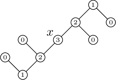
Observe that \(\mathsf{T}(x)\) is a finite tree with the path \((x)\) as root. As before, Given \(\rho \sqsubseteq \rho'\), we write \(\rho' - \rho\) for the final segment of \(\rho'\) after \(\rho\). Moreover, we write \({\uparrow}(\rho' - \rho)\) if each element in \(\rho' - \rho\) covers its predecessor in \(\rho'\), and \({\downarrow}(\rho' - \rho)\) if each element in \(\rho' - \rho\) is covered by its predecessor in \(\rho'\). For \(\rho \in \mathsf{ZZP}(x)\), the height of \(\rho\) is defined as \(h(\rho) \mathrel{\vcenter{:}}= \max\{\lvert \rho' - \rho \rvert \mid \rho \sqsubseteq \rho'\}\).
We now define, for \(x\) in a finite, acyclic labelled poset, the simulation formulas \(\chi^+(x)\) and \(\chi^-(x)\), which together encode all worlds accessible from \(x\) via a non-repeating path. Therefore, satisfying or falsifying \(\chi^+(x)\) or \(\chi^-(x)\) respectively at some world \(y\) of a labelled poset is equivalent to the existence of a simulation involving \(x\) and \(y\); see Proposition 6.7.
We define \(\chi^+(x)\) and \(\chi^-(x)\) by working ‘outside-in’ on \(\mathsf{T}(x)\), i.e. recursively from the leaves of \(\mathsf T(x)\) to the root, exploiting the following.
By asserting a formula \(\varphi \mathbin{\tikz[baseline=-.5ex] \draw[-to reversed] (0,0) -- (1em,0);}\psi\) we can express that there is a world below where \(\varphi\) holds and \(\psi\) does not.
By denying a formula \(\varphi \rightarrow \psi\) we can express that there is a world above where \(\varphi\) holds and \(\psi\) does not.
We begin by defining for each path \(\rho\) in \(\mathsf T(x)\) different from \((x)\) a formula \(\varphi_\rho\). The simulation formulas are then composed from these formulas \(\varphi_\rho\). Recall that by convention \(\bigwedge \emptyset \mathrel{\vcenter{:}}= \top\) and \(\bigvee \emptyset \mathrel{\vcenter{:}}= \bot\).
Definition 6.21. Let \(\mathcal{X}=(X, \leq_\mathcal{X}, \ell_\mathcal{X})\) be a finite, acyclic \(\Sigma\)-labelled poset, and \(x \in X\). For each \(\rho = (\rho(0), \ldots, \rho(n)) \in \mathsf T(x)\) with \(\lvert \rho \rvert > 0\) define the formula \(\varphi_\rho\) by induction on \(h(\rho)\). Suppose \(\varphi_\rho'\) has been defined for each \(\rho'\) with \(h(\rho') < h(\rho)\).
If \(\rho(n-1) >_\mathcal{X} \rho(n)\), define \[\begin{align} \varphi_\rho \mathrel{\vcenter{:}}= &(\bigwedge \ell_\mathcal{X}(\rho(n))^+ \wedge \bigwedge_{\rho' \sqsupset \rho \colon {\downarrow}(\rho' - \rho)} \varphi_{\rho'}) \mathbin{\tikz[baseline=-.5ex] \draw[-to reversed] (0,0) -- (1em,0);}\\&(\bigvee \ell_\mathcal{X} (\rho(n))^- \vee \bigvee_{\rho' \sqsupset \rho \colon {\uparrow}(\rho' - \rho)} \varphi_{\rho'}) \end{align}\]
If \(\rho(n-1) <_\mathcal{X} \rho(n)\), define \[\begin{align} \varphi_\rho \mathrel{\vcenter{:}}= & (\bigwedge \ell_\mathcal{X}(\rho(n))^+ \wedge \bigwedge_{\rho' \sqsupset \rho \colon {\downarrow}(\rho' - \rho)} \varphi_{\rho'}) \rightarrow \\& (\bigvee \ell_\mathcal{X} (\rho(n))^- \vee \bigvee_{\rho' \sqsupset \rho \colon {\uparrow}(\rho' - \rho)} \varphi_{\rho'}) \end{align}\]
Then define \(\chi^+(x)\) and \(\chi^-(x)\) as follows.
\[\begin{align} \chi^+(x) \mathrel{\vcenter{:}}= &(\bigwedge \ell_\mathcal{X}(x)^+ \wedge \bigwedge_{\rho \sqsupset (x) \colon {\downarrow}(\rho - (x))} \varphi_{\rho}) \mathbin{\tikz[baseline=-.5ex] \draw[-to reversed] (0,0) -- (1em,0);}\\&(\bigvee \ell_\mathcal{X} (x)^- \vee \bigvee_{\rho \sqsupset (x) \colon {\uparrow}(\rho - (x))} \varphi_{\rho}) \end{align}\]
\[\begin{align} \chi^-(x) \mathrel{\vcenter{:}}= &(\bigwedge \ell_\mathcal{X}(x)^+ \wedge \bigwedge_{\rho \sqsupset (x) \colon {\downarrow}(\rho - (x))} \varphi_{\rho}) \rightarrow \\&(\bigvee \ell_\mathcal{X}(x)^- \vee \bigvee_{\rho \sqsupset (x) \colon {\uparrow}(\rho -(x))} \varphi_{\rho}) \end{align}\]
For a path \(\rho = (\rho(i))_{i\leq n}\) let \(\mathbf{f}(\rho) \mathrel{\vcenter{:}}= \rho(n)\), i.e. \(\mathbf{f}(\rho)\) denotes the final element of \(\rho\). Let \[\mathbf{f}[\mathsf{ZZP}(x)] = \{ \mathbf{f}(\rho) \mid \rho \in \mathsf{ZZP}(x)\}.\]
Recall that \(\mathcal{M}_\mathrm{c} = (W_\mathrm{c},{\leq_\mathrm{c}},f_\mathrm{c},V_\mathrm{c})\) is the canonical model. Moreover, recall that by Lemma 6.8 if \(\varphi \rightarrow \psi \not \in \Gamma\) for \(\Gamma \in W_c\), then there exists \(\Delta \in W_c\) with \(\Gamma \leq_c \Delta\) and \(\varphi \in \Delta\) and \(\psi \not \in \Delta\). Similarly, if \(\varphi \mathbin{\tikz[baseline=-.5ex] \draw[-to reversed] (0,0) -- (1em,0);}\psi \in \Gamma\), then there exists \(\Delta \in W_c\) with \(\Delta \leq_c \Gamma\) and \(\varphi \in \Delta\) and \(\psi \not \in \Delta\).
Proposition 6.7. Let \(\frac{\mathcal{M}_\mathrm{c}}{\Sigma} = (U ,{\leq},R,\ell)\) and \(E_* \subseteq U\times W_\mathrm{c}\) be the strongly surjective dynamic simulation provided by Proposition 6.6. Let \(x \in U\) and \(\Gamma \in W_\mathrm c\). The following hold.
\(\chi^+(x) \in \Gamma\) if and only if there exists \(\Delta \in W_\mathrm c\) with \(\Delta \leq_\mathrm{c} \Gamma\) such that \(x \mathrel E_* \Delta\).
\(\chi^-(x) \in \mathcal{L}_\mathsf{biLTL}\setminus \Gamma\) if and only if there exists \(\Delta \in W_\mathrm c\) with \(\Gamma \leq_\mathrm c \Delta\) such that \(x\mathrel E_* \Delta\).
Proof. We first prove the left-to-right direction of [condition43] and [condition-]. Given a path \(\rho\), denote by \((\varphi_\rho)_\mathsf{L}\) the subformula on the left of \(\varphi_\rho\)’s principal connective and by \((\varphi_\rho)_\mathsf{R}\) the subformula on the right. Define a function \(f: \mathbf{f}[\mathsf{ZZP}(x)] \longrightarrow W_c\) satisfying for all \(\rho \in \mathsf{ZZP}(x)\) the property \[\label{equation32simulation32formulas} (\varphi_\rho)_\mathsf{L} \in f(\mathbf{f}(\rho)) \text{ and } (\varphi_\rho)_\mathsf{R} \in f(\mathbf{f}(\rho))^c\tag{16}\] (where \(\Delta^c = \mathcal{L}_\mathsf{biLTL}\setminus \Delta\) for \(\Delta \in W_c\)) by induction on \(\lvert \rho \rvert\) as follows, where we assume that for \((x)\) the formula \(\varphi_{(x)} = \chi^+(x)\) or \(\varphi_{(x)} = \chi^-(x)\), for [condition43] and [condition-], respectively. For the base case observe that if \(\rho \in \mathsf{ZZP}(x)\) and \(\lvert \rho \rvert = 0\), then \(\rho = (x)\). For [condition43], by assumption \(\chi^+(x) \in \Gamma\), so there exists a world \(\Delta \leq_c \Gamma\) such that \((\chi^+(x))_\mathsf{L} \in \Delta\) and \((\chi^+(x))_\mathsf{R} \in \Delta^c\). Define \(f(x) = \Delta\). For [condition-], by assumption \(\chi^-(x) \not \in \Gamma\), so there exists a world \(\Delta \geq_c \Gamma\) such that \((\chi^-(x))_{\mathsf{L}} \in \Delta\) and \((\chi^-(x))_{\mathsf{R}} \in \Delta^c\). Again, define \(f(x) = \Delta\).
For the induction step suppose that \(f\) has been defined for all \(\rho\) with \(\lvert \rho \rvert \leq n\) and satisfies 16 . Let \(\rho \in \mathsf{ZZP}(x)\) with \(\lvert \rho \rvert = n+1\). Let \(\rho' \sqsubset \rho\) be the unique path such that \(\lvert \rho - \rho'\rvert = 1\). We distinguish the following two cases.
First, suppose \(\mathbf{f}(\rho') < \mathbf{f}(\rho)\). Then the principal connective of \(\varphi_\rho\) is an implication. Observe that \(\varphi_\rho\) is a subformula of \(\varphi_{\rho'}\) occurring on the right-hand side of the principal connective. By the induction hypothesis and the properties of a type, we have \(\varphi_\rho \in(\mathbf{f}(\rho'))^c\). Hence there exists a world \(\Delta \in W_c\) with \(f(\mathbf{f}(\rho')) \leq_c \Delta\) and \((\varphi_\rho)_\mathsf{L} \in \Delta\) and \((\varphi_\rho)_\mathsf{R} \in \Delta^c\). Define \(f(\mathbf{f}(\rho)) \mathrel{\vcenter{:}}= \Delta\).
Otherwise \(\mathbf{f} (\rho') > \mathbf{f}(\rho)\). Then the principal connective of \(\varphi_\rho\) is a co-implication and \(\varphi_\rho\) is a subformula of \(\varphi_{\rho'}\) occurring on the left-hand side of the principal connective. By the induction hypothesis and the properties of a type, we have \(\varphi_\rho \in f(\mathbf{f}(\rho')\). Hence there exists a world \(\Delta \in W_c\) with \(\Delta \leq_c f(\mathbf{f}(\rho'))\) and \((\varphi_\rho)_\mathsf{L} \in \Delta\) and \((\varphi_\rho)_\mathsf{R} \in \Delta^c\). Define \(f(\mathbf{f}(\rho)) \mathrel{\vcenter{:}}= \Delta\).
We claim that \(f \subseteq U \times W_c\) is a simulation. Let \((u, f(u)) \in f\) for arbitrary \(u \in \mathbf{f}[\mathsf{ZZP}(x)]\). Let \(\rho\) be the unique path with \(\mathbf{f}(\rho)=u\). We check that all three conditions of a simulation are satisfied.
1. By property 16 , \((\varphi_{\rho})_{\mathsf{L}} \in f(u)\) and \((\varphi_{\rho})_{\mathsf{R}} \in f(u)^c\). Since \(\bigwedge \ell_\mathcal{X}(u)^+\) is a subformula of \((\varphi_\rho)_L\) it follows from the properties of a type that \(\ell_\mathcal{X}(u)^+ \subseteq f(u)\). Similarly, since \(\bigvee \ell_\mathcal{X}(u)^-\) is a subformula of \((\varphi_\rho)_{\mathsf{R}}\) it follows that \(\ell_\mathcal{X}(u)^- \subseteq f(u)^c\). Therefore \(\ell_\mathcal{X}(u) \subseteq_\mathrm{T} (f(u), f(u)^c)\).
2. Suppose \(u \leq u'\). First suppose that \(u'\) covers \(u\). Let \(\rho' \in \mathsf{ZZP}(x)\) be the unique path with \(\mathbf{f}(\rho') = u'\). There are two cases to consider: either \(\rho \sqsubset \rho'\) or \(\rho' \sqsubset \rho\). In both cases it follows immediately from construction that \(f(u) \leq_c f(u')\), and hence that there exists \(\Delta \in W_c\) with \(f(u) \leq_c \Delta\) and \((u', \Delta) \in f\). In case \(u \leq u'\) but \(u'\) does not cover \(u\), the result follows by induction on the number of worlds between \(u\) and \(u'\), using the above argument in the induction step (the base case is trivial).
3. Suppose \(u' \leq_\mathcal{X} u\). The argument is then symmetrical to the previous case.
Therefore, \(f\) is a simulation relating \(x\) with \(\Delta\) for some \(\Delta \in W_c\) with \(\Delta \leq_c \Gamma\). Since \(E_*\) is the union of all simulation between \(\frac{\mathcal{M}_\mathrm{c}}{\Sigma}\) and \(\mathcal{M}_c\), we obtain that \(x \mathrel{E_*} \Delta\).
Next, we prove the right-to-left direction of [condition43] and [condition-]. To that end we show by induction on the height of \(\rho\) that whenever \(\mathbf{f}(\rho) \mathrel{E_*} \Delta\), then \[\label{equation32simulation32formulas322} (\varphi_\rho)_{\mathsf{L}} \in \Delta \text{ and } (\varphi_\rho)_{\mathsf{R}} \in \Delta^c.\tag{17}\]
For the base suppose \(h(\rho) = 0\). Then \(\mathbf{f}(\rho) = u\) is a leaf of \(\mathsf{ZZP}(x)\). Let \(u \mathrel{E_*} \Delta\) for some \(\Delta \in W_c\). By definition of a simulation \(\ell(u)^+ \subseteq \Delta\) and \(\ell(u)^- \subseteq \Delta^c\), implying that \[\label{equation32simulation32formulas323} \bigwedge \ell(u)^+ \in \Delta \text{ and } \bigvee \ell(u)^- \in \Delta^c.\tag{18}\]
The claim then follows from observing that \((\varphi_\rho)_{\mathsf{L}} = \bigwedge \ell(u)^+\) and \((\varphi_\rho)_{\mathsf{R}} = \bigvee \ell(u)^-\).
For the induction step suppose that (17 ) holds for all \(\rho'\) with \(h(\rho') \leq n\) and suppose \(h(\rho) = n+1\). Let \(\mathbf{f}(\rho) = u\) and \(u \mathrel{E_*} \Delta\). First, note that (18 ) holds for \(u\) by the same argument as before. Now suppose \(\rho \sqsubset \rho'\) and \({\downarrow}(\rho' - \rho)\). Let \(\mathbf{f}(\rho') = u'\). Then \(u' < u\), and so by forth-down confluence there exists \(\Delta' \in W_c\) with \(\Delta' \leq_c \Delta\) and \(u' \mathrel{E_*} \Delta'\). Note that \(h(\rho') \leq n\). Thus by induction hypothesis we have \((\varphi_{\rho'})_\mathsf{L} \in \Delta'\) and \((\varphi_{\rho'})_\mathsf{R} \in (\Delta')^c\). Let \(\rho' = (\rho'(i))_{i \leq k}\). Then \(\rho'(k-1) > \rho'(k) = u'\), since \(\rho \sqsubset \rho'\) and \({\downarrow}(\rho' - \rho)\). Therefore the main connective of \(\varphi_{\rho'}\) is a co-implication. Thus by Lemma 6.8 we have that \(\varphi_{\rho'} \in \Delta\). Next, suppose \(\rho \sqsubset \rho'\) and \({\uparrow}(\rho' - \rho)\). Then, by a similar argument, we find \(u < \mathbf{f}(\rho') = u' \mathrel{E_*} \Delta'\) and \(\Delta \leq_c \Delta'\). By induction hypothesis \((\varphi_{\rho'})_\mathsf{L} \in \Delta'\) and \((\varphi_{\rho'})_\mathsf{R} \in (\Delta')^c\). Since the main connective of \(\varphi_{\rho'}\) is an implication, we conclude that \(\varphi_{\rho'} \in \Delta^c\) by Lemma 6.8. Thus, by properties of a type, we have \((\varphi_\rho)_{\mathsf{L}} \in \Delta\) and \((\varphi_\rho)_\mathsf{R} \in \Delta^c\).
Finally, suppose \(\varphi_{(x)} = \chi^+(x)\) and there exists \(\Gamma, \Delta \in W_c\) with \(\Delta \leq_c \Gamma\) and \(x \mathrel{E_*} \Delta\). By the above proof \(\chi(x)^+_{\mathsf{L}} \in \Delta\) and \(\chi(x)^+_{\mathsf{R}} \in \Delta^c\). By Lemma 6.8 we conclude that \(\chi^+(x) \in \Gamma\). Similarly if \(\varphi_{(x)} = \chi^-(x)\) and there exists \(\Gamma, \Delta \in W_c\) with \(\Gamma \leq_c \Delta\) and \(x \mathrel{E_*} \Delta\), then by the above proof \(\chi(x)^-_{\mathsf{L}} \in \Delta\) and \(\chi(x)^-_{\mathsf{R}} \in \Delta^c\). Thus Lemma 6.8 implies that \(\chi^-(x) \in \Gamma^c\). ◻
Next we establish some \(\mathsf{biLTL}\)-derivable properties of \(\chi^+\) and \(\chi^-\). We begin with the former. These properties are established by using Proposition 6.7 to see that they are present in every prime theory in the canonical model and so derivable. As before, \(\frac{\mathcal{M}_\mathrm{c}}{\Sigma}= (U ,{\leq},R,\ell)\); the reflexive transitive closure of \(R\) is denoted \(R^*\).
Proposition 6.8. Given \(w \in U\) and \(\psi\in \Sigma\), the following hold.
If \(\psi\in \ell({{w}})^-\), then \(\vdash \chi^+(w)\rightarrow (\chi^+(w) \mathbin{\tikz[baseline=-.5ex] \draw[-to reversed] (0,0) -- (1em,0);}\psi ).\)
If \(\psi\in \ell({w})^+\), then \(\vdash \chi^+(w) \rightarrow \psi.\)
\(\vdash\displaystyle \chi^+(w) \rightarrow \mathbin{{\bigcirc}}\bigvee _{{{w}} \mathrel{R}{{{v}}} } \chi^+(v).\)
Proof. [itPropsubplOne]. Let \(\Gamma\in W_\mathrm{c}\) and assume that \(\psi\in \ell(w)^-\) and \(\chi^+(w) \in \Gamma\). By properties of the canonical model, it suffices to show that \(\chi^+(w) \mathbin{\tikz[baseline=-.5ex] \draw[-to reversed] (0,0) -- (1em,0);}\psi \in \Gamma\). From \(\chi^+(w) \in \Gamma\) and Proposition 6.7, case [condition43], we obtain \(\Delta\leq_\mathrm{c} \Gamma\) such that \(w \mathrel{E_*} \Delta\). Hence \(\psi\in \Delta^c\) and, using Proposition 6.7, case [condition43], in the opposite direction, \(\chi^+(w) \in \Delta\). These yield \(\chi^+(w) \mathbin{\tikz[baseline=-.5ex] \draw[-to reversed] (0,0) -- (1em,0);}\psi \in \Gamma\).
[itPropsubplOneb]. If \(\psi\in \ell ({w})^+\), as above, let \(\Gamma\in W_\mathrm{c}\) be such that \(\chi^+(w) \in \Gamma^+\), and \(\Delta\leq_\mathrm{c} \Gamma\) with \(w \mathrel{E_*} \Delta\). Then \(\psi\in\Delta\), yielding \(\psi\in \Gamma\).
[itPropsubplFive]. Let \(\Gamma\) be such that \(\chi(w)^+ \in \Gamma\), so there exists \(\Delta\leq_\mathrm{c} \Gamma\) with \(w\mathrel E_* \Delta\). Since \(E_*\) is dynamic, there is \(v\) such that \(w\mathrel R v\) and \(v\mathrel E_* f_\mathrm{c}(\Delta)\). By Proposition 6.7, we have \(\chi^+(v) \in f_\mathrm{c} ( \Delta )\), which implies that \(\mathbin{{\bigcirc}}\chi^+(v) \in \Delta\). Thus \(\mathbin{{\bigcirc}}\chi^+(v) \in \Gamma\) by definition of \(\leq_\mathrm{c}\), so \(\mathbin{{\bigcirc}}\bigvee_{w\mathrel R v} \chi^+(v) \in \Gamma^+\). ◻
The formula \(\chi^-\) behaves ‘dually’, as follows.
Proposition 6.9. Given \(w \in U\) and \(\psi\in \Sigma\), the following hold.
If \(\psi\in \ell({w})^+\), then \(\vdash (\psi \rightarrow \chi^-(w) )\rightarrow \chi^-(w)\).
If \(\psi\in \ell({{w}})^-\), then \(\vdash \psi\rightarrow \chi^-(w)\).
\(\vdash\displaystyle \mathbin{{\bigcirc}}\bigwedge _{{{w}} \mathrel R {{{v}}} } \chi^-(v) \rightarrow \chi^-(w).\)
Proof. [itPropsubOneb]. Suppose that \(\psi\in \ell ({w})^+\). We prove the claim by contraposition. If \(\chi(w)^- \in \Gamma^c\) for some \(\Gamma\in W_\mathrm{c}\), then there is \(\Delta \geq _\mathrm{c} \Gamma\) such that \(w \mathrel{E_*} \Delta\). But then \(\chi^-(w)\in \Delta^c\) and \(\psi\in \Delta\), which implies that \(\psi\rightarrow\chi^-(w) \in \Delta^c\); hence also \(\psi\rightarrow\chi^-(w) \in \Gamma^c\), as required.
[itPropsubOne]. Assume that \(\psi\in \ell ({w})^- \cap \Gamma\), and suppose that \(\Delta \in W_c\) is such that \(w \mathrel{ E_*} \Delta\). Then \(\psi\in \Delta^c\), which means we cannot have \(\Delta \geq_c \Gamma\). Hence Proposition 6.7 implies that \(\chi^-(w)\notin \Gamma^c\), i.e. \(\chi^-(w)\in \Gamma\).
[itPropsubFive]. Proceed by contraposition. If \(\chi^-(w)\in \Gamma^c\) for some \(\Gamma\in W_\mathrm{c}\), then there is \(\Delta\geq _\mathrm{c}\Gamma\) such that \(w \mathrel E_* \Delta\) by Proposition 6.7. Since \(E_*\) is dynamic, there is \(v\in U\) such that \(w\mathrel R v\) and \(v\mathrel E_ * f_\mathrm{c}(\Delta)\). Thus \(\chi^- (v) \in f_\mathrm{c}(\Delta)^c\); hence \(\mathbin{{\bigcirc}}\chi^-(v) \in \Delta^c\), and by downward persistence, \(\mathbin{{\bigcirc}}\chi^-(v) \in \Gamma^c\). Hence \(\mathbin{{\bigcirc}}\bigwedge_{w\mathrel R v} \chi^- (v) \in \Gamma^c\). ◻
6.11 Completeness↩︎
The simulation formulas \(\chi^+\) and \(\chi^-\) are fundamental in the completeness proof. Specifically, they will be used to show that \(\frac{\mathcal{M}_\mathrm{c}}{\Sigma}\) is \(\omega\)-sensible and hence a quasimodel. Since validity over the class of quasimodels is equivalent to validity over the class of expanding models by Theorem 6.4, completeness will follow. The following lemma is the first step towards establishing \(\omega\)-sensibility. As above, we write \(\frac{\mathcal{M}_\mathrm{c}}{\Sigma}= (U,{\leq},R,\ell)\) and \(R^*\) for the reflexive transitive closure of \(R\), and \(E_* \subseteq U\times W_\mathrm{c}\) is the strongly surjective dynamic simulation between \(\frac{\mathcal{M}_\mathrm{c}}{\Sigma}\) and \(\mathcal{M}_c\), where \(\mathcal{M}_c\) is the canonical model. As in the completeness proof for \(\mathrm{IM_{H}}\) in Chapter 3, let \(R^*(w)\) be the reachable component of \(w\), i.e. \(R^*(w) = \{ v \in U \mid w \mathrel{R}^* v\}\). In order to show that \(\frac{\mathcal{M}_\mathrm{c}}{\Sigma}\) is \(\omega\)-sensible, we need to use formal induction over the reachable component of worlds. The following lemma will help us achieve this.
Lemma 6.20. If \(\Sigma\subseteq \mathcal{L}_\mathsf{biLTL}\) is finite and closed under subformulas, and \({{w}}\in U\), then:
\(\vdash \bigvee _{w \mathrel R^* v}\chi^+({{{v}}}) \rightarrow \mathbin{{\bigcirc}}\bigvee _{w \mathrel R^* v}\chi^+(v)\),
\(\vdash \mathbin{{\bigcirc}}\bigwedge _{w \mathrel R^* v}\chi^-(v)\rightarrow \bigwedge _{w \mathrel R^* v}\chi^-({{{v}}})\).
Proof. The first item follows from Proposition 6.8, case [itPropsubplFive], as for any \(w \mathrel{R^*}v\) we have that \[\vdash \chi^+({{{v}}}) \rightarrow \mathbin{{\bigcirc}}\bigvee _{v \mathrel R u}\chi^+(u) .\] Since \(v \mathrel R u\) implies that \(w \mathrel R^ * u\), \[\vdash \chi^+({{{v}}}) \rightarrow \mathbin{{\bigcirc}}\bigvee _{w \mathrel R^* u}\chi^+(u) .\] Since \(v\) was arbitrary, we obtain \[\vdash \bigvee _{w \mathrel R^* v}\chi^+({{{v}}}) \rightarrow \mathbin{{\bigcirc}}\bigvee _{w \mathrel R^* u}\chi^+(u),\] which by a change of variables yields the original claim.
Item 2 is similar, but uses Proposition 6.9, case [itPropsubFive]. ◻
In order to complete our proof that \(\frac{\mathcal{M}_\mathrm{c}}{\Sigma}\) is \(\omega\)-sensible, it suffices to apply the induction rules \(\mathsf{Ind}_{\mathbin{\Box}}\) and \(\mathsf{Ind}_{\Diamond}\) of our calculus to the formulas of Lemma 6.20.
Proposition 6.10 (\(\omega\)-sensibility).
If \({{w}}\in U\) and \(\Diamond\psi\in \ell ({{w}})^+\), then there exists \({{{v}}}\in{R^*}({{w}})\) such that \(\psi\in \ell ({{{v}}})^+\).
If \({{w}}\in U\) and \(\mathbin{\Box}\psi\in \ell ({{w}})^-\), then there exists \({{{v}}}\in{R^*}({{w}})\) such that \(\psi\in \ell({{{v}}})^-\).
Proof. [ittempincone] . Towards a contradiction, assume that \({{w}}\in U\) and \(\Diamond\psi\in \ell ({{w}})^+\), but for all \({{{v}}}\in{R^*}({{w}})\), we have \(\psi \in \ell({{v}})^-\). By Lemma 6.20, \(\vdash \mathbin{{\bigcirc}}\bigwedge \limits_{w \mathrel R^* v} \chi^-({{{v}}})\rightarrow \bigwedge\limits_{w \mathrel R^* v} \chi^-({{{v}}})\). By the \(\mathsf{Ind}_\Diamond\) rule, \({\vdash \Diamond\bigwedge \limits_{w \mathrel R^* v} \chi^-({{{v}}})}\rightarrow \bigwedge\limits_{w \mathrel R^* v} \chi^-({{{v}}})\); in particular, \[\label{other} \vdash \Diamond\bigwedge _{w\mathrel R^* v} \chi^-({{{v}}})\rightarrow \chi^-({{w}}).\tag{19}\]
Now let \({{{v}}}\in{R^*}({{w}})\). By Proposition 6.9, case [itPropsubOne], and the assumption that \(\psi \in \ell({{{v}}})^-\), we have that \(\vdash \psi \rightarrow \chi^-({{{v}}})\), and since \({{{v}}}\) was arbitrary, \(\vdash \psi \rightarrow \bigwedge_{w\mathrel R^* v}\chi^-({{{v}}})\). Using \(\mathsf{Mon}_\Diamond\), we further have that \(\vdash \Diamond\psi \rightarrow \Diamond\bigwedge_{w\mathrel R^* v}\chi^-({{{v}}})\). This, along with (19 ), shows that \(\vdash \Diamond\psi \rightarrow \chi^-({{w}})\). However, by Proposition 6.9, case [itPropsubOneb], and our assumption that \(\Diamond\psi\in \ell ({{w}})^+\), we have that \(\vdash ( \Diamond\psi \rightarrow \chi^-({{w}}) ) \rightarrow \chi^-(w)\). Hence by \(\mathsf{MP}\) we obtain \(\vdash \chi^-({{w}}).\) Choosing \(\Gamma\in W_\mathrm c\) such that \(w\mathrel E_*\Gamma\), Proposition 6.7, case [condition-], yields \(\chi^-({{w}}) \notin\Gamma\), but this contradicts \(\vdash \chi^-({{w}})\). We conclude that there is \({{{v}}}\in{R^*}({{w}})\) with \(\psi \in \ell({{v}})^+\), as needed.
[ittempinctwo]. This is similar to the first item, but dualised. Towards a contradiction, assume that \({{w}}\in U\) and \(\mathbin{\Box}\psi\in \ell ({{w}})^-\) but, for all \({{{v}}}\in{R^*}({{w}})\), we have \(\psi \in \ell({{w}})^+\). By Lemma 6.20, \(\vdash \bigvee \limits_{w \mathrel R^* v} \chi^+({{{v}}}) \rightarrow \mathbin{{\bigcirc}}\bigvee \limits_{w \mathrel R^* v} \chi^+({{{v}}})\). By the \(\mathsf{Ind}_{\mathbin{\Box}}\)-rule, \(\vdash \bigvee \limits_{w \mathrel R^* v} \chi^+({{{v}}})\rightarrow\Box \bigvee \limits_{w \mathrel R^* v} \chi^+({{{v}}})\); in particular, \[\label{otherb} \vdash\chi^+({{w}}) \rightarrow \mathbin{\Box}\bigvee _{w\mathrel R^*v} \chi^+({{{v}}}) .\tag{20}\]
Now let \({{{v}}}\in{R^*}({{w}})\). By Proposition 6.8, case [itPropsubplOneb], and the assumption that \(\psi \in \ell({{{v}}})^+\), we have that \(\vdash \chi^+({{{v}}}) \rightarrow \psi\), and since \({{{v}}}\) was arbitrary, \(\vdash \bigvee_{w\mathrel R^* v}\chi^+({{{v}}})\rightarrow \psi\). Using \(\mathsf{Mon}_{\mathbin{\Box}}\) we further have that \(\vdash \mathbin{\Box}\bigvee_{w\mathrel R^* v}\chi^+({{{v}}}) \rightarrow \mathbin{\Box}\psi\). This, along with (20 ), shows that \[\label{eqPlusBox} \vdash \chi^+({{w}}) \rightarrow \mathbin{\Box}\psi.\tag{21}\] By Proposition 6.8, case [itPropsubplOne] and our assumption that \(\mathbin{\Box}\psi\in \ell ({{w}})^-\), we have that \(\vdash \chi^+(w) \rightarrow ( \chi^+({{w}}) \mathbin{\tikz[baseline=-.5ex] \draw[-to reversed] (0,0) -- (1em,0);}\mathbin{\Box}\psi )\). Hence by 21 and Lemma 6.2, case [itDimpMon], we obtain \(\vdash \chi^+({{w}}) \rightarrow (\mathbin{\Box}\psi\mathbin{\tikz[baseline=-.5ex] \draw[-to reversed] (0,0) -- (1em,0);}\mathbin{\Box}\psi).\) Since \((\mathbin{\Box}\psi\mathbin{\tikz[baseline=-.5ex] \draw[-to reversed] (0,0) -- (1em,0);}\mathbin{\Box}\psi) \equiv\bot\), this implies that \(\chi^+({{w}})\) is contradictory. Choosing \(w\in U\) such that \(w \mathrel E_* \Gamma\), Proposition 6.7, case [condition43], yields \(\chi^+({{w}}) \in\Gamma\), which once again is impossible and we conclude that there is \({{{v}}}\in{R^*}({{w}})\) with \(\psi \in \ell({{v}})^-\). ◻
Corollary 6.1. If \(\Sigma\subseteq \mathcal{L}_\mathsf{biLTL}\) is finite and closed under subformulas, then \(\frac{\mathcal{M}_\mathrm{c}}{\Sigma}\) is a quasimodel.
Proof. By Proposition 6.6, \(\frac{\mathcal{M}_\mathrm{c}}{\Sigma}\) is a labelled system (and serial, since \(\mathcal{M}_\mathrm c\) is), while by Proposition 6.10, \(R\) is \(\omega\)-sensible. So by Definition 6.12, \(\frac{\mathcal{M}_\mathrm{c}}{\Sigma}\) is a quasimodel. ◻
We are now ready to prove that our calculus is complete.
Theorem 6.11. Given \(\varphi \in \mathcal{L}_\mathsf{biLTL}\), the following are equivalent:
\(\mathsf{biLTL}\vdash\varphi\),
\(\varphi\) is valid over the class of expanding models,
\(\varphi\) is valid over the class of finite quasimodels.
Proof. That [itOne] implies [itTwo] is Theorem 6.2 and that [itTwo] implies [itThree] is Theorem 6.4. We show that [itThree] implies [itOne] by contraposition. Suppose \(\varphi\) is an unprovable formula and let \(\Sigma\) be the set of subformulas of \(\varphi\). Since \(\varphi\) is unprovable, there exists \(\Gamma\in W_\mathrm{c}\) with \(\varphi\notin\Gamma\). Since \(E_*\) is strongly surjective, there is \(w\in U\) such that \(\varphi\in\ell(w)^-\) and \(w\mathrel E_* \Gamma\). Hence \(w\) is a point in a finite quasimodel falsifying \(\varphi\). ◻
Corollary 6.2. Derivability in \(\mathsf{biLTL}\) is decidable.
This follows from the fact that \(\mathsf{biLTL}\) is axiomatisable and has a finite quasimodel property (with a computable bound on the ‘finite’).
6.12 Conclusion↩︎
The main contribution of this chapter is the presented sound and complete axiomatization for bi-intuitionistic linear temporal logic. This is the first finite axiomatization for a logic extending intuitionistic linear temporal logic over the full temporal language including ‘next’, ‘eventually’ and ‘henceforth’ and thus solves a long standing open problem. Our method of proving completeness was based on the finite model construction from Chapter [c: bi-int ml new] which was used to obtain a finite ‘filtrated’ model which embeds into the canonical model via a dynamic simulation. The proof is thereby an interesting adaptation of classical techniques for LTL to the intuitionistic realm, illustrating in particular the significant increase in the difficulty of the mathematical theory. The crucial ingredient for obtaining a complete axiomatization is the co-implication, whose presence is exploited to prove \(\mathsf{iLTL}\)-validites such as the \(\mathbf{RV}\)-formula. As a consequence we noted that the axiomatization is not conservative over the \(\mathbin{\tikz[baseline=-.5ex] \draw[-to reversed] (0,0) -- (1em,0);}\)-free fragment of the logic. In the completeness proof the co-implication is crucial in establishing that the modal accessibility relation of \(\frac{\mathcal{M}_\mathrm{c}}{\Sigma}\) is \(\omega\)-sensible for \(\mathbin{\Box}\) case (while implication was used to prove the \(\Diamond\) case). This leads us to the first question left open by our work:
Question 6.1. Can \(\mathsf{iLTL}\) over the full language be finitely axiomatized without the co-implication?
We are optimistic that this is indeed possible, partly due to the fact that Menéndez Turata managed to obtain a sound and complete cyclic proof system for \(\mathsf{iLTL}\) over the full language [24], which might be used to extract a finite axiomatization. We leave this problem for future work.
An interesting corollary of this chapter is that \(\mathbin{\tikz[baseline=-.5ex] \draw[-to reversed] (0,0) -- (1em,0);}\) cannot be extended to the class of topological models while validating bi-intuitionistic logic, since as verified in [86], this would mean that the class of dynamic topological models would validate \(\mathsf{biLTL}\), and hence validate \(\mathbf{RV}\), which we know by Example 6.1 not to be the case.
Corollary 6.3. Suppose that \(\mathbin{\tikz[baseline=-.5ex] \draw[-to reversed] (0,0) -- (1em,0);}_\mathrm{top}\) assigns to each topological space \((X,\tau)\) a binary operation \(\tau \times \tau \to \tau\). (Here, \(\tau\) is the collection of opens.) Consider the semantics that combines standard topological semantics for intuitionistic propositional logic with \(\mathbin{\tikz[baseline=-.5ex] \draw[-to reversed] (0,0) -- (1em,0);}_\mathrm{top}\) semantics for \(\mathbin{\tikz[baseline=-.5ex] \draw[-to reversed] (0,0) -- (1em,0);}\). Then the class of topological spaces does not validate propositional bi-intuitionistic logic.
A natural next step to extend our work would be to turn to proof theory with the aim of developing an analytic sequent calculus for bi-intuitionistic linear temporal logic. This is a follow up problem to Question [q: proof theory for biml]: an analytic sequent calculus for bi-intuitionistic modal logic could be extended by fixed point rules, admitting analytic non-wellfounded proofs. However, this would require to combine nested sequents with non-wellfounded branches, which is notoriously difficult to handle (see Question 4.1).
7 English Summary↩︎
This thesis develops the mathematical theory of intuitionistic dynamic logics - extensions of intuitionistic propositional logic with modalities and fixed point operators. Such systems provide formal tools for reasoning about change, such as encountered in mathematical systems evolving over time or in the knowledge state of an agent after an information update.
We investigate five intuitionistic dynamic logics: intuitionistic master modality, intuitionistic common knowledge logic, intuitionistic linear temporal logic, bi-intuitionistic modal logic and bi-intuitionistic linear temporal logic. On the proof theoretic side we develop sound and complete Hilbert-style axiomatizations as well as non-wellfounded and cyclic sequent calculi. On the semantic side we study these logics over various classes of dynamic models, which are birelational Kripke models satisfying confluence and frame conditions. We establish expressivity results, the finite model property, decidability, as well as complexity bounds.
The main contributions are threefold. First, we develop analytic cyclic sequent calculi for intuitionistic master modality and common knowledge logic, where completeness is obtained by a robust proof search argument. Second, we obtain the finite model property and decidability for bi-intuitionistic modal logic via an intricate combinatorial analysis of dynamic models. Third, we develop a sound and complete axiomatization for intuitionistic linear temporal logic featuring the temporal operators next, eventually and henceforth, thereby providing a positive answer to the long-standing open question concerning the existence of a finite axiomatization.
8 Nederlandstalige Samenvatting↩︎
Dit proefschrift ontwikkelt de wiskundige theorie van intuïtionistische dynamische logica’s — uitbreidingen van de intuïtionistische propositionele logica met modaliteiten en fixpunt-operatoren. Dergelijke systemen bieden formele instrumenten om te redeneren over verandering, zoals die optreedt in wiskundige systemen die in de tijd evolueren of in de kennistoestand van een agent na een informatie-update.
We onderzoeken vijf intuïtionistische dynamische logica’s: intuïtionistische meestermodaliteit, intuïtionistische gemeenschappelijke-kennislogica, intuïtionistische lineaire temporele logica, bi-intuïtionistische modale logica en bi-intuïtionistische lineaire temporele logica. Aan de bewijstheoretische kant ontwikkelen we correcte en volledige Hilbert-stijl-axiomatiseringen, evenals niet-welgegronde en cyclische sequent-calculi. Aan de semantische kant bestuderen we deze logica’s over verschillende klassen van dynamische modellen, dat wil zeggen birelationele Kripke-modellen die voldoen aan confluentie en framecondities. We bewijzen resultaten over expressiviteit, de eindig-model-eigenschap, beslisbaarheid en complexiteitsgrenzen.
De belangrijkste bijdragen zijn drievoudig. Ten eerste ontwikkelen we analytische cyclische sequent-calculi voor intuïtionistische meestermodaliteit en gemeenschappelijke-kennislogica, waarbij volledigheid wordt verkregen via een robuust bewijszoek-argument. Ten tweede verkrijgen we de eindig-model-eigenschap en beslisbaarheid voor de bi-intuïtionistische modale logica door middel van een verfijnde combinatorische analyse van dynamische modellen. Ten derde ontwikkelen we een correcte en volledige axiomatisering voor de intuïtionistische lineaire temporele logica met de temporele operatoren next, eventually en henceforth, waarmee een positief antwoord wordt gegeven op de lang openstaande vraag naar het bestaan van een eindige axiomatisering.
References↩︎
We also use \(\leq\) for the standard smaller-equal relation on the set of natural numbers. Note that \(\leq\) is a well-order on \(\omega\).↩︎
Technically speaking, the displayed graph is a frame and not a model, since the valuation is not displayed. Since whenever a frame is depicted, the valuation is provided in the example, we do not make this distinction here.↩︎
However, there are some exceptions, for example the choice rules employed in Chapter 3.↩︎
Technically, since sequents are ordered pairs of sets of formulas, formulas can serve simultaneously as principal and as side formulas in a rule instance. In such an instance the principal formula also occurs in the premises. Thus it is possible to always continue the proof search even if only finitely many sequents occur; however, such strategy for proof search is hardly reasonable.↩︎
In that case one needs to be careful with the inductive definition of the language to guarantee that every formula induces a monotone function.↩︎
Observe that \(u_0\) might be identical to \(\pi_n(y)\). Nevertheless, we add a fresh world \(y_0\) to \(I_n\) which in this case would be a copy of \(y\).↩︎
It might be that at step \(m > n\) a \(\larger[-1.5]\square\)-defect situated at a world \(x\) in \(I_n\) is resolved. But in that case the construction first adds a new world above \(x\) and then a modal successor for that new world. The case for \(\ooalign{\larger[-1.5]\square\cr \hidewidth\raise.035ex* \mkern 1.12mu\cr}\)-defects is similar.↩︎
A semantic analysis immediately shows that the other direction, i.e. \(\vdash \larger[-1.5]\square(\varphi \vee \psi) \rightarrow (\larger[-1.5]\square\varphi \vee \larger[-1.5]\square\psi)\), should not* hold. The soundness theorem (c.f. Theorem 3.4) will confirm this intuition.*↩︎
This is a semantic notion of invertibility.↩︎
Although the calculus \(\mathrm{nIM}\) is only used to show completeness of \(\mathrm{cIM}\), let us note here that \(\mathrm{nIM}\) is also sound: this follows from soundness of \(\mathrm{cIM}\) and Lemma 3.32.↩︎
Since \(\mathcal{M}\) is a triangle model, we have \(w \mathrel{(R \circ {\leq})} v\). However, in the refutation \(v\) does not contain a node which is a modal premise of the same \(\mathsf{C_t}\)-rule instance of which \(t_w\) is a conclusion of. Therefore this additional case has to be considered.↩︎
If \(\ooalign{\larger[-1.5]\square\cr \hidewidth\raise.035ex* \mkern 1.12mu\cr}\varphi\) is unfocused, then the saturation clause 7. guarantees this. Otherwise the saturation clause 8. guarantees it. In the second case, there exists a node \(s \in w\) with \(\ooalign{\larger[-1.5]\square\cr \hidewidth\raise.035ex* \mkern 1.12mu\cr}\varphi^f \in \Delta_s\). Since \(\ooalign{\larger[-1.5]\square\cr \hidewidth\raise.035ex* \mkern 1.12mu\cr}\varphi^f\) cannot occur in \(\Delta_{t_w}\), there must be a (non-preserving) application of \(\ooalign{\larger[-1.5]\square\cr \hidewidth\raise.035ex* \mkern 1.12mu\cr}\mathsf{R}\) with \(\ooalign{\larger[-1.5]\square\cr \hidewidth\raise.035ex* \mkern 1.12mu\cr}\varphi^f\) as principal formula.↩︎
This requires \(f\) to be a total function, as otherwise there could be maximal worlds in \(\leq\) which have no successor.↩︎
For the interested reader who is unwilling to try out the many possible and sensible candidates for a proof, let us remark here that both possible sequents in the premise are invalid. Thus the soundness result presented in the next section will provide an alternative and simpler proof.↩︎
We will close every canonical model under triangle confluence and not mention it in the next cases.↩︎
We use different names for the system and some of the rules than [22].↩︎
This will not be mentioned again henceforth.↩︎
Formally, a trace \((\varphi_i)_{i}\) passes degeneratively through \(\mathbin{\mathsf{U}}\mathrm{L}\) if there is a \(\varphi_j\) of the form \(\varphi\mathbin{\mathsf{U}}\psi^n\) such that \(\varphi_{j+1}\in\{\varphi^n,\psi^n\}\).↩︎
If the reader has skipped Chapter 3, it may be informative to go back and briefly review the key ideas presented there.↩︎
Note that this is essentially what was done in the completeness proof for \(\mathrm{IM_H}\), but we defined \(\frac{\mathcal{M}_c}{\sim}\) directly instead of via a filtration.↩︎
We will always close \(\leq_{n+1}\) under transitivity and reflexivity and will not mention it in the following items.↩︎