CDS: Counterfactual Directionality Score for Structured Interventions in Spatial Graphs
July 15, 2026
Abstract
Quantifying directional influence between node populations is a fundamental problem in graph-based modeling, particularly in spatial biological systems where cell–cell interactions shape functional outcomes. Existing approaches based on attention, attribution, or correlation capture associations but do not provide a principled framework for evaluating directional effects under controlled perturbations. We introduce a framework for structured counterfactual interventions in graph-based models to estimate directional influence between node types. Our approach trains a Neighbor Influence Model (NIM) to predict node states from local neighborhoods and applies constrained interventions that modify neighborhood composition while preserving key spatial and structural properties. We define the Counterfactual Directionality Score (CDS), which measures the change in predicted node state induced by targeted perturbations, and provide a theoretical interpretation of CDS as a finite-difference measure of local intervention sensitivity. To obtain valid uncertainty estimates, we introduce a core-level bootstrap procedure that accounts for dependencies within spatial samples. Experiments on synthetic spatial graphs with known directional structure show that CDS recovers directional influence, remains well calibrated under null conditions, and is robust to confounding signals, while preliminary results on spatial transcriptomics data reveal biologically plausible and consistent interactions across tissue cores.
1 Introduction↩︎
Spatially-resolved single-cell technologies reveal how cells interact within tissues. A central question is directional influence: how does one cell type affect the molecular state of another? Answering this question is key to understanding tumor–immune interactions, stromal remodeling, and signaling in health and disease. Graph neural networks (GNNs) model such data by representing cells as nodes and spatial proximity as edges. While GNNs achieve strong predictive performance, they provide limited tools for quantifying directional effects between cell populations. Existing approaches, such as attention weights, feature attribution, and correlation-based cell–cell interaction analyses, capture associations but often fail to distinguish true directional influence from confounding factors such as shared microenvironmental signals or global expression trends.
We introduce a framework for structured counterfactual interventions in graph-based models to estimate directional influence. Our principle is: if a sender population influences a receiver’s state, systematically removing that population should change the receiver’s predicted cellular state. We operationalize this idea by training a Neighbor Influence Model (NIM) that predicts a cell’s transcriptomic state from its spatial neighborhood. Then we apply counterfactual interventions that modify neighborhood composition while preserving key spatial and structural constraints, including neighborhood size, spatial weighting, and tissue context. The resulting Counterfactual Directionality Score (CDS) quantifies the sensitivity of a receiver’s predicted state to targeted perturbations. We further introduce within‑type interventions as an empirical baseline to distinguish the effects of cell‑type presence from individual cell‑state variability. We provide a theoretical interpretation of CDS as a finite-difference measure of local intervention sensitivity under structured neighborhood perturbations. Our structured interventions isolate compositional effects while controlling for structural confounders. To obtain valid uncertainty estimates, we develop a core‑level bootstrap procedure that accounts for dependencies within tissue samples.
On synthetic spatial graphs with known directional structure, CDS recovers ground truth directional structure, remains well calibrated under null conditions, and is robust to confounding signals. Compared to baseline methods, CDS uniquely combines sensitivity to true interactions with robustness to spurious correlations. Preliminary results on spatial transcriptomics datasets show that CDS identifies biologically plausible sender–receiver relationships with consistent behavior across tissue cores.
1.0.0.1 Contributions.
Our main contributions are: (1) a framework for structured counterfactual interventions in spatial graphs that preserves key structural properties; (2) CDS, a model-based measure of directional influence between cell types; (3) a theoretical characterization of CDS as a finite-difference intervention measure under structured perturbations; (4) a core-level bootstrap procedure for statistically principled inference; and (5) empirical validation showing that CDS recovers directional structure, remains well calibrated under null conditions, and is robust to confounding.
2 Related Work↩︎
Our work connects several research areas: interpretability for graph neural networks, attention-based models, computational methods for cell–cell interaction inference, and causal machine learning with counterfactual reasoning.
Several methods have been developed to explain predictions of GNNs. GNNExplainer [1] identifies compact subgraphs and node features that are most influential for a GNN’s predictions. PGExplainer [2] provides a parameterized approach that efficiently generates explanations for multiple instances. While these methods reveal which graph components are important, they focus on attribution rather than estimating directional effects between node populations. Our CDS explicitly perturbs neighbourhood composition in a structured way to estimate directional influence.
Attention mechanisms in GNNs, such as Graph Attention Networks (GATs) [3], learn adaptive weights over neighbours and have been used to interpret which interactions are “important”. However, attention weights reflect correlations within the observed data distribution and do not provide a counterfactual characterization of directionality. Our work instead uses explicit counterfactual interventions to isolate the effect of a specific cell type’s presence.
In computational biology, tools such as CellPhoneDB [4] and NicheNet [5] infer ligand–receptor interactions from single-cell and spatial transcriptomics data using prior knowledge of molecular interactions. More recent spatial CCI methods [6], [7] incorporate spatial proximity to score interactions. Though these methods are powerful for hypothesis generation, they are primarily correlation-based or rely on curated databases. Our framework is model-agnostic and learns a predictive model of cell state from neighbourhood composition. This enables principled counterfactual estimation without requiring predefined interaction databases.
Causal inference provides a formal language for estimating intervention effects [8]. In machine learning, counterfactual explanations have been applied to image and tabular data (e.g., [9]). For graphs, recent work has proposed counterfactual graph generation for model explanation (e.g., [10]), but these approaches typically modify graph structure globally or focus on graph-level classification. To our knowledge, our work is the first to combine a learned graph-based surrogate model with spatially constrained, cell-type-specific counterfactual interventions to estimate directional influence between node populations in spatial biological graphs. The core-level bootstrap further provides statistically principled inference that respects the dependence structure of tissue samples.
3 Problem Setup↩︎
We consider a spatially-resolved single-cell dataset represented as a graph \(G = (V, E)\), where each node \(i \in V\) corresponds to a cell, and edges \((i,j) \in E\) encode spatial proximity between cells. Each cell is associated with (1) a feature vector \(x_i \in \mathbb{R}^p\) representing its transcriptomic state, and (2) a discrete cell-type label \(\tau(i) \in \mathcal{T}\). Let \(X \in \mathbb{R}^{|V| \times p}\) denote the matrix of all cell features.
3.0.0.1 Spatial neighborhood.
For each cell \(i\), we define a local neighborhood \(N(i) \subset V\) based on spatial proximity. In practice, \(N(i)\) may be constructed via \(k\)-nearest neighbors in physical space, but our formulation is agnostic to the specific construction as long as it captures local cell–cell interactions.
3.0.0.2 Sender and receiver populations.
For a pair of cell types \((s, r) \in \mathcal{T}^2\), we define the sender and receiver populations: \[\begin{align} S &= \{ i \in V : \tau(i) = s \}, \\ R &= \{ i \in V : \tau(i) = r \}. \end{align}\]
3.0.0.3 Interaction-driven cell state.
We view the observed transcriptomic state of a receiver cell \(i \in R\) as the result of both intrinsic factors and extrinsic influences from its local neighborhood: \[x_i = f\big(x_i^{\mathrm{int}}, \{x_j : j \in N(i)\}\big) + \epsilon_i\] where \(x_i^{\mathrm{int}}\) denotes intrinsic (cell-autonomous) components and the neighborhood term captures microenvironmental influence. \(\epsilon_i\) captures unmodeled variability.
3.0.0.4 Problem objective.
Our goal is to quantify the directional influence of sender-type cells on receiver-type cells. Formally, for each receiver cell \(i \in R\), we define a neighborhood composition variable \(Z_i^{(s)}\) that summarizes the contribution of sender-type cells in \(N(i)\). We are interested in estimating the effect: \[\Delta_i^{(s \to r)} = f\big(x_i^{\mathrm{int}}, Z_i^{(s)}\big) - f\big(x_i^{\mathrm{int}}, 0\big),\] which represents the change in the receiver cell state induced by removing sender-type cells from the local neighborhood.
3.0.0.5 Scientific question.
This formulation allows us to address the central question: Do neighboring sender-type cells influence the transcriptomic program of receiver-type cells, and if so, what is the magnitude and direction of this effect?
4 Neighbor Influence Model↩︎
4.1 Distance-Weighted Neighborhood Aggregation↩︎
We model the influence of a cell’s local microenvironment through a distance-weighted aggregation of its neighbors. For each cell \(i\) and neighbor \(j \in N(i)\), let \(d_{ij}\) denote their Euclidean distance in tissue space. We define normalized weights: \[w_{ij} = \frac{\exp\bigl(-d_{ij} / \alpha\bigr)}{\sum_{j' \in N(i)} \exp\bigl(-d_{ij'} / \alpha\bigr)}, \label{eq:softmax95weights95clean}\tag{1}\] where \(\alpha > 0\) controls the spatial decay of influence.
Using these weights, we define the neighborhood representation \(a_i \in \mathbb{R}^p\): \[a_i = \sum_{j \in N(i)} w_{ij} x_j.\]
4.2 Modeling Neighborhood Influence↩︎
We approximate the unknown function \(f\) introduced in Section 3 using a graph-based parametric model \(f_\theta\), referred to as NIM: \[\hat{z}_i = f_\theta(a_i, \tau(i)) \in \mathbb{R}^p. \label{eq:nim95output95clean}\tag{2}\]
The model takes as input the neighborhood representation \(a_i\) and the receiver cell type \(\tau(i)\), and predicts the receiver’s transcriptomic state. Learning \(f_\theta\) provides a data-driven estimate of how local neighborhood composition maps to cellular gene expression.
4.2.0.1 Architecture.
\(f_\theta\) is implemented as a multi-layer feedforward network with residual connections. The input \(a_i\) is projected into a latent space, processed by \(L\) residual blocks, and modulated by a cell-type-conditioned gating mechanism. Specifically, each cell type \(\tau(i)\) is embedded into a vector \(e_{\tau(i)}\), which is transformed into a feature-wise gate: \[g_i = \sigma(W_{\mathrm{type}} e_{\tau(i)} + b_{\mathrm{type}}),\] that multiplicatively modulates the hidden representation.
This gating allows the model to capture heterogeneous response functions, i.e., different receiver cell types may respond differently to the same neighborhood signal.
4.3 Training Objective↩︎
We train \(f_\theta\) to minimize the discrepancy between predictions \(\hat{z}_i\) and observed states \(x_i\) using the Huber loss: \[\mathcal{L}(\theta) = \frac{1}{|\mathcal{B}|} \sum_{i \in \mathcal{B}} \ell_\delta(\hat{z}_i, x_i),\] where \(\ell_\delta\) is defined as the Huber loss.
4.3.0.1 Interpretation.
A low prediction error implies that neighborhood composition contains predictive information about the receiver cell state. Importantly, this learned mapping \(f_\theta\) serves as a surrogate model for evaluating counterfactual neighborhood perturbations (Section 6), enabling estimation of sensitivity to sender-to-receiver perturbations.
5 CDS↩︎
5.1 Intuition↩︎
While NIM captures how neighborhood composition predicts cell state, it does not by itself identify which neighboring cell types drive this effect. To address this, we introduce CDS, which measures the sensitivity of a receiver cell’s predicted state to targeted perturbations of its neighborhood.
5.2 Counterfactual Predictions↩︎
Let \(f_\theta\) be the trained NIM. For a receiver cell \(i\), the original prediction is: \[\hat{z}_i = f_\theta(a_i, \tau(i)),\] where \(a_i\) is the original neighborhood aggregation.
We construct a counterfactual neighborhood \(N^{\mathrm{cf}}(i)\) via an intervention operator \(\mathcal{I}_{S \rightarrow R}\) that modifies the presence of sender-type cells while preserving the spatial weighting structure. The corresponding counterfactual prediction is: \[\hat{z}_i^{\mathrm{cf}} = f_\theta(a_i^{\mathrm{cf}}, \tau(i)),\] where \(a_i^{\mathrm{cf}}\) denotes the neighborhood aggregation computed from the counterfactual neighborhood \(N^{\mathrm{cf}}(i)\).
5.3 Intervention Operators↩︎
We define two structured intervention operators that modify neighborhood composition while preserving key spatial and structural properties. These interventions are designed to isolate the contribution of sender-type cells to receiver predictions.
5.3.0.1 Type-Swap Intervention.
This operator removes the presence of sender-type cells from the receiver’s neighborhood. For each receiver \(i \in R\) and each neighbor \(j \in N(i)\) with \(\tau(j) = s\), we replace \(j\) with a cell \(j'\) sampled from the same tissue core such that \(\tau(j') \neq s\).
To ensure physically plausible perturbations, we perform distance-bin-preserving replacement. The \(k\) neighbor slots are partitioned into spatial bins based on distance, and each sender slot is preferentially replaced by a non-sender cell from the same bin; if no such candidate exists, the search expands to nearby bins.
This construction preserves three structural invariants:
Degree preservation: \(|N^{\mathrm{cf}}(i)| = |N(i)| = k\).
Microenvironment consistency: replacement cells are drawn from the same tissue core as \(i\).
Distance-slot preservation: spatial weights \(\{w_{ij}\}\) remain unchanged, so differences between \(a_i\) and \(a_i^{\mathrm{cf}}\) arise solely from changes in neighborhood composition.
As a result, changes in prediction are attributable primarily to changes in neighborhood composition rather than artifacts of graph structure or spatial weighting.
5.3.0.2 Within-Type Intervention.
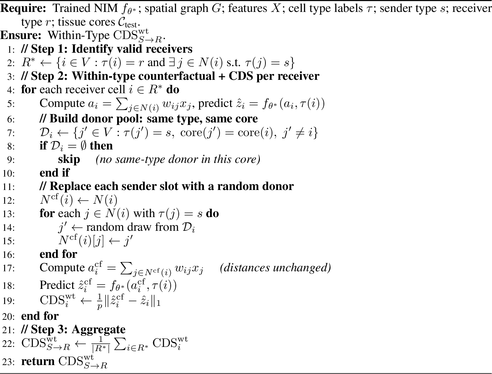
This operator help characterize the effect of sender cell identity while preserving sender cell type. For each sender neighbor \(j \in N(i)\) with \(\tau(j) = s\), we replace \(j\) with a different cell \(j'\) of the same type, drawn from the donor pool: \[\mathcal{D}_i = \bigl\{\, j' \in V : \tau(j') = s,\; \mathrm{core}(j') = \mathrm{core}(i),\; j' \neq i \,\bigr\}.\]
If \(\mathcal{D}_i = \emptyset\), the receiver \(i\) is excluded from analysis. This intervention preserves the presence of sender-type cells while randomizing which specific cells occupy neighborhood slots.
5.4 CDS Definition↩︎
For each receiver cell \(i\), we define: \[\mathrm{CDS}_i = \frac{1}{p} \left\| \hat{z}_i^{\mathrm{cf}} - \hat{z}_i \right\|_1.\] This measures the average change in predicted state under the counterfactual intervention.
A larger \(\mathrm{CDS}_i\) indicates that the perturbed cell type substantially influences the receiver’s transcriptomic state.
We also define a signed variant: \[\mathrm{CDS}_i^{\mathrm{sgn}} = \frac{1}{p} \sum_{m=1}^{p} \bigl(\hat{z}_{i,m}^{\mathrm{cf}} - \hat{z}_{i,m}\bigr),\] which captures the direction of influence (upregulation vs.suppression).
Finally, we aggregate over receiver cells: \[\mathrm{CDS}_{S \rightarrow R} = \frac{1}{|R^*|} \sum_{i \in R^*} \mathrm{CDS}_i,\] where \(R^*\) includes receivers for which the intervention is valid.
5.4.0.1 Interpretation.
CDS provides a model-based measure of directional influence: it quantifies how much the predicted state of receiver cells depends on the presence or identity of sender-type cells in their local neighborhood.
6 Theoretical Properties of Counterfactual Directionality↩︎
CDS can be interpreted as a finite-difference measure of the sensitivity of model predictions to structured neighborhood perturbations. The difference \(a_i^{\mathrm{cf}} - a_i\) captures changes in neighborhood composition induced by the intervention while preserving spatial structure and neighborhood size.
Structured interventions preserve neighborhood size, spatial distances (and therefore weights \(w_{ij}\)), and receiver type, so \[a_i^{\mathrm{cf}} - a_i = \sum_{m \in N(i)} w_{im} \bigl(x_m^{\mathrm{cf}} - x_m\bigr),\] thereby separating compositional changes from changes in graph topology.
Under within-type exchangeability, \[\mathbb{E}[a_i^{\mathrm{cf}} - a_i] = 0,\] providing an empirical null baseline. Because CDS depends on the aggregated neighborhood representation \(a_i\), it captures only effects mediated through this representation. If \(f_\theta\) is \(L\)-Lipschitz, then \[\mathrm{CDS}_i \leq \frac{L}{p} \|a_i^{\mathrm{cf}} - a_i\|_2.\]
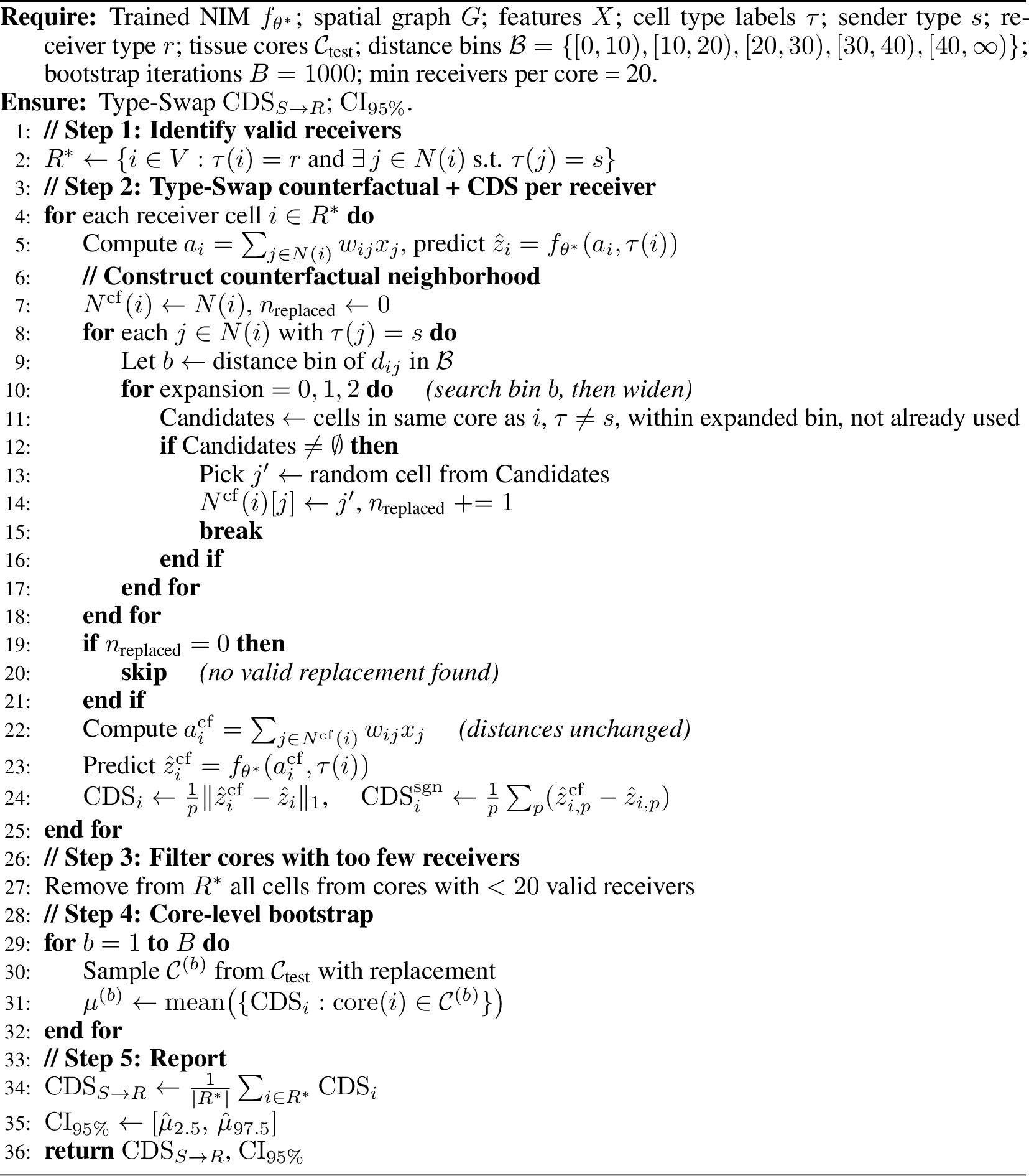
For statistical inference, we use a core-level bootstrap procedure: we resample \(M\) tissue cores with replacement, compute bootstrap means \(\mu^{(b)}\), and construct percentile confidence intervals to account for dependence within tissue cores.
6.0.0.1 Implementation.
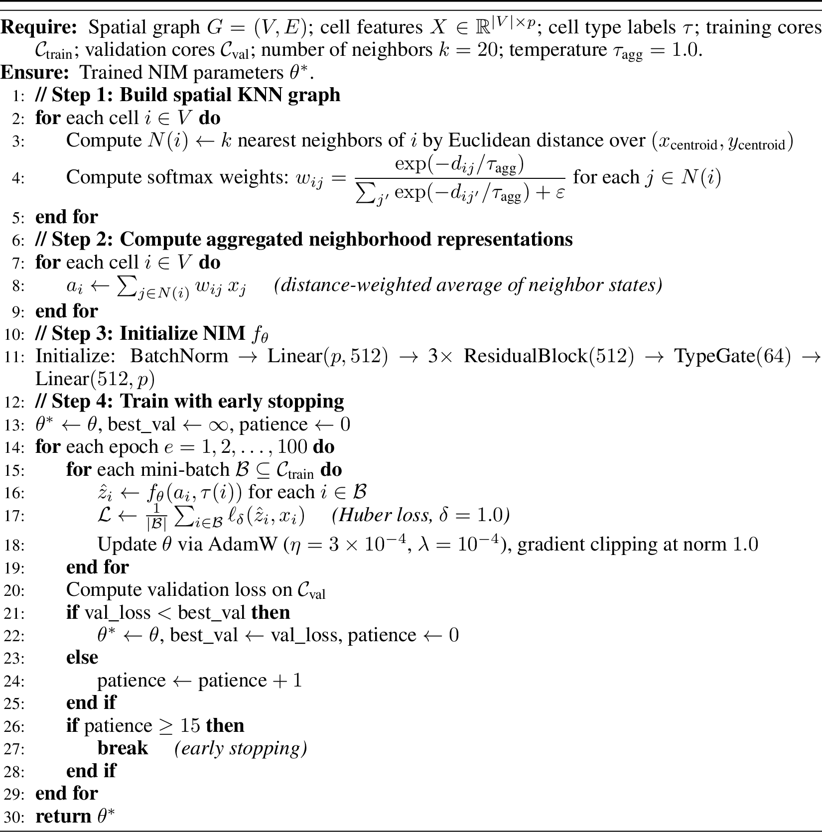
We train NIM using standard optimization procedures and compute CDS via structured counterfactual perturbations of local neighborhoods. Full algorithmic details are provided in Appendix 9.
7 Experiments↩︎
We evaluate whether CDS recovers directional influence under controlled synthetic settings and compare it against standard attribution and perturbation baselines. Our evaluation focuses on directionality, robustness to confounding, and stability. These experiments empirically validate the theoretical properties of CDS derived in Section 6, including its sensitivity to neighborhood perturbations and robustness under null exchangeability.
7.1 Experimental Setup↩︎
7.1.0.1 Synthetic Spatial Generator
We construct spatial graphs with three cell types: sender (\(S\)), receiver (\(R\)), and background (\(B\)). Cell coordinates are sampled uniformly and a \(k\)-nearest neighbor graph is built with distance-based softmax weights.
Receiver features are generated under three regimes:
Positive (true influence): \[z_i = \mu_R + a_i W + \epsilon,\] where \(\mu_R \in \mathbb{R}^p\) is a receiver-type baseline expression vector, \(a_i\) is the weighted aggregation of neighboring sender features, \(W \in \mathbb{R}^{p \times p}\) controls sender-to-receiver influence strength, and \(\epsilon \sim \mathcal{N}(0,\sigma^2 I)\) is Gaussian noise.
Null (no influence): \[z_i \sim \mathcal{N}(\mu_R, \sigma^2 I),\] independent of neighboring cells.
Spurious (confounded): A shared latent variable induces correlation across cell types without local directional influence.
This design preserves feature marginals while controlling the underlying directional dependency structure.
7.1.0.2 Predictive Model
We train NIM, a residual neural network that predicts cell features from neighborhood aggregates with cell-type gating. CDS is computed by comparing model predictions under original and counterfactual neighborhoods constructed via constrained neighbor replacement.
7.2 Synthetic Validation↩︎
7.2.0.1 Directional Recovery
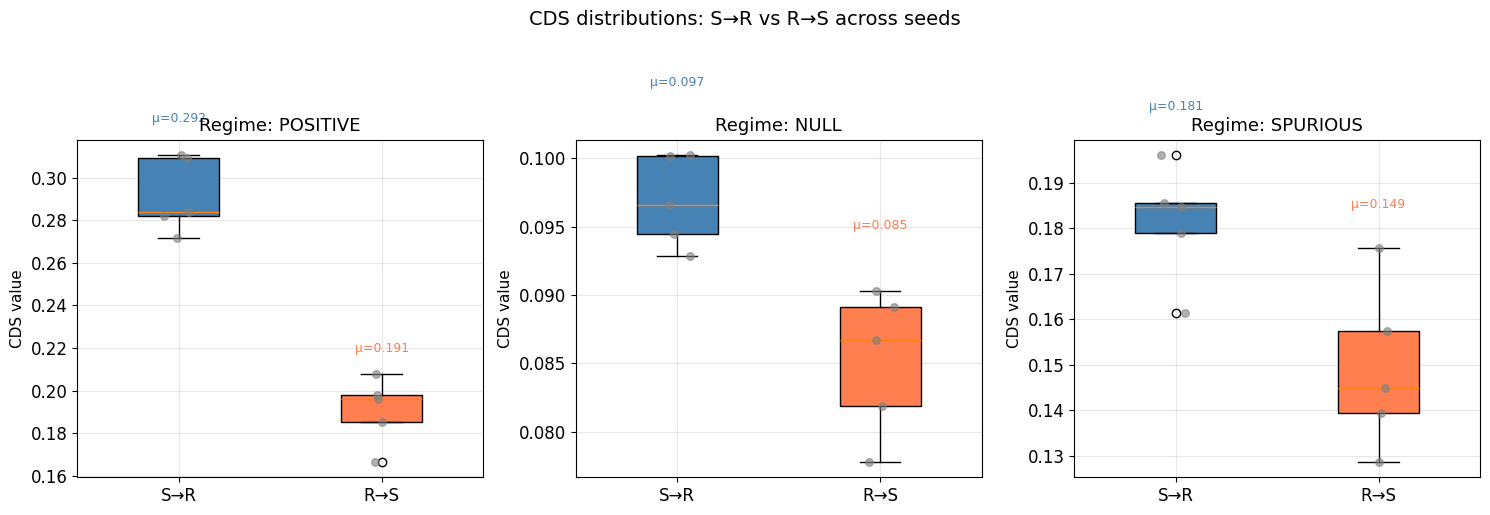
We first evaluate whether CDS correctly recovers directional structure under controlled synthetic settings. Figure 1 shows that in the positive regime, CDS consistently assigns higher values to the true direction (\(S \rightarrow R\)) than the reverse (\(R \rightarrow S\)) across all noise levels and random seeds. This gap remains stable as noise increases, indicating that the learned model captures directional dependencies rather than symmetric correlations. In contrast, in the null regime, both directions yield near-zero CDS values, confirming that the method does not produce spurious directional signal (Table 1) and is well calibrated in the absence of true interaction.
7.2.0.2 Null Control
Under the null setting, where receiver features are independent of neighboring sender cells, CDS values collapse to near zero for both directions (Table 1), confirming that the method does not introduce spurious directional signal under null conditions.
7.2.0.3 Spurious Correlation Control
To test robustness to confounding, we introduce a shared latent signal affecting all cell types. As shown in Figure 1 and Table 1, CDS values remain lower than in the positive regime, and the directional gap is reduced.
This indicates that CDS preferentially captures structured local influence rather than global correlations, and does not incorrectly attribute strong directional effects under confounding.
7.3 Quantitative Evaluation↩︎
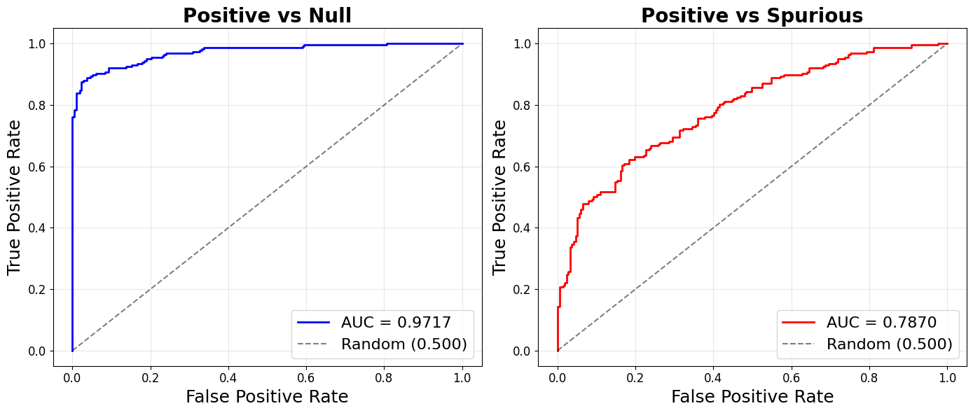
We evaluate the ability of CDS to distinguish true interaction from null and confounded settings using ROC analysis. As shown in Figure 2, CDS achieves high AUC for distinguishing positive from null regimes (AUC = 0.97) and maintains above-chance discrimination under confounding (AUC = 0.79). These results indicate that CDS captures structured directional signals beyond simple correlation-based separation. Table 1 summarizes CDS magnitude and stability across regimes. In the positive setting, CDS is substantially larger than in null and spurious regimes, with a low coefficient of variation across bootstrap samples. Bootstrap analysis further shows that CDS estimates are tightly concentrated, with narrow confidence intervals, indicating stable estimation across tissue cores. We compare CDS against random perturbation and gradient sensitivity baselines (Table 2). CDS consistently achieves higher scores in the positive regime while remaining near zero under null conditions.
| Regime | CDS (S→R) | CDS (R→S) | AUC vs. Positive | Stability (CV) |
|---|---|---|---|---|
| Positive | \(0.2915 \pm 0.0156\) | \(0.1907 \pm 0.0140\) | — | \(0.034 \pm 0.016\) |
| Null | \(0.0969 \pm 0.0030\) | \(0.0852 \pm 0.0047\) | 0.970 | \(0.023 \pm 0.009\) |
| Spurious | \(0.1813 \pm 0.0114\) | \(0.1492 \pm 0.0161\) | 0.793 | \(0.055 \pm 0.014\) |
| Method | Positive | Null | Spurious |
|---|---|---|---|
| CDS (ours) | \(0.272 \pm 0.016\) | \(0.099 \pm 0.003\) | \(0.176 \pm 0.011\) |
| Gradient | \(0.104 \pm 0.012\) | \(0.039 \pm 0.005\) | \(0.045 \pm 0.007\) |
| Random | \(0.098 \pm 0.008\) | \(0.097 \pm 0.009\) | \(0.095 \pm 0.010\) |
| Method | CDS | Drop (%) | CV | Receivers |
|---|---|---|---|---|
| Full method | 0.269 | 0.0 | 0.027 | 217 |
| Unmatched donor replacement | 0.286 | -5.5 | 0.013 | 240 |
| No distance preservation | 0.216 | 20.6 | 0.027 | 217 |
| No within-type baseline | 0.272 | 0.0 | 0.034 | 217 |
7.4 Ablation Study↩︎
We evaluate the importance of structural constraints in the counterfactual intervention. Table 3 shows that removing degree preservation, distance preservation, or within-type baseline correction alters CDS magnitude and increases variability relative to the full method. In particular, unmatched donor replacement introduces variability by altering neighborhood composition, while removing distance preservation disrupts spatial weighting, leading to noisier estimates. These results are consistent with the theoretical motivation for the structured intervention design (Section 6) and suggest that preserving neighborhood structure improves the stability and specificity of CDS estimates.
7.5 Robustness Analysis↩︎
7.5.0.1 Noise and Interaction Robustness.
As observation noise increases, CDS magnitude decreases but the directional gap between \(S \rightarrow R\) and \(R \rightarrow S\) persists, showing graceful degradation. Core-level bootstrap yields low variance and tight confidence intervals, confirming stability (Figure 3). Increasing ground-truth interaction strength produces monotonic increases in CDS, consistent with the finite-difference sensitivity interpretation of CDS (Section 6).
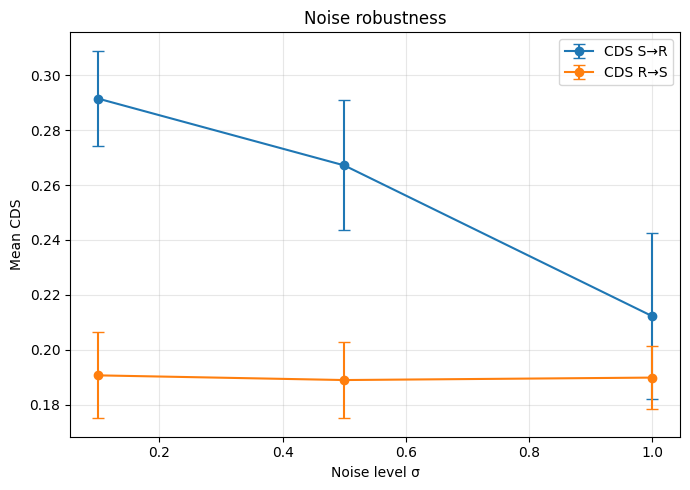
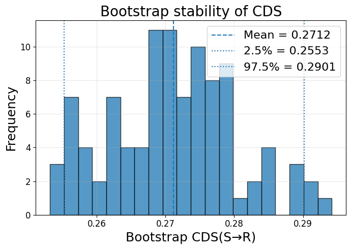
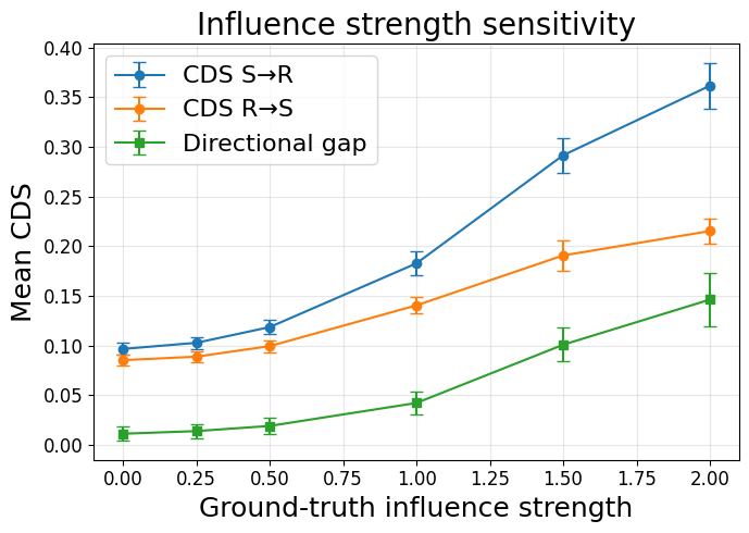
Figure 3: Robustness analysis of CDS. (a) Noise robustness: mean \(\mathrm{CDS}_{S \rightarrow R}\) and \(\mathrm{CDS}_{R \rightarrow S}\) across increasing observation noise. (b) Bootstrap stability: distribution of bootstrap CDS estimates across resampled tissue cores. (c) Influence-strength sensitivity: CDS as a function of ground-truth sender-to-receiver interaction strength..
7.6 Real-World Data↩︎
We applied our CDS framework to two independent spatial transcriptomics datasets: breast cancer (BRCA) and lung cancer tissue microarrays [11]. For each dataset, we considered three major cell populations: Tumor, Stromal, and Immune—resulting in four directional hypotheses, namely, Tumor\(\rightarrow\)Stromal, Stromal\(\rightarrow\)Tumor, Tumor\(\rightarrow\)Immune, and Stromal\(\rightarrow\)Immune. We trained separate NIMs for each cancer type using the same architecture and hyperparameters, computed CDS via type-swap interventions with core-level bootstrap validation (1000 iterations; 3 test cores per cancer type), and report mean CDS values with 95% bootstrap confidence intervals.
Figure 4 shows CDS estimates for all four sender–receiver pairs in BRCA and lung cancer. Tumor\(\rightarrow\)Stromal influence (CDS = 0.0715 [0.0550, 0.0758]) substantially exceeded Stromal\(\rightarrow\)Tumor influence (CDS = 0.0247 [0.0191, 0.0271]), indicating asymmetric directional signaling from malignant to stromal compartments. We observed similar moderate scores for Tumor\(\rightarrow\)Immune (0.0657 [0.0598, 0.0677]) and Stromal\(\rightarrow\)Immune (0.0687 [0.0576, 0.0784]), suggesting that immune cell states are influenced by both tumor and stromal microenvironments. The confidence intervals for Tumor\(\rightarrow\)Stromal and Stromal\(\rightarrow\)Tumor do not overlap, providing evidence for directional asymmetry.
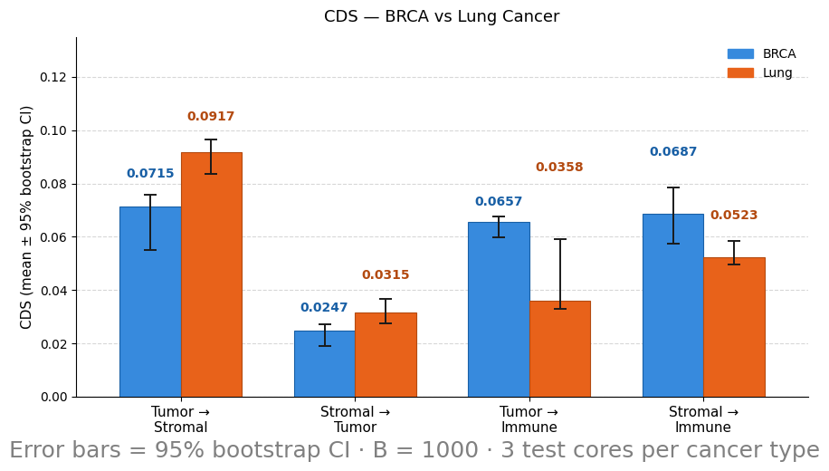
In the lung tissue, a clear directional signature can be seen (Figure 4). Tumor\(\rightarrow\)Stromal influence (0.0917 [0.0837, 0.0965]) was again the strongest observed effect, exceeding the BRCA magnitude and showing the largest directional gap relative to Stromal\(\rightarrow\)Tumor (0.0315 [0.0277, 0.0368]). However, immune-related interactions diverged from BRCA: Tumor\(\rightarrow\)Immune (0.0358 [0.0328, 0.0591]) and Stromal\(\rightarrow\)Immune (0.0523 [0.0495, 0.0583]) were substantially lower in lung. This suggests tissue-specific immune interaction patterns. The Stromal\(\rightarrow\)Immune signal remained moderately elevated relative to Tumor\(\rightarrow\)Immune, a pattern reversed from BRCA. Higher immune-directed CDS values in BRCA than in lung suggest that the framework captures biologically plausible differences in tumor–immune crosstalk across cancer contexts.
8 Conclusion↩︎
We introduced CDS, a framework for structured counterfactual interventions in spatial graphs to quantify directional influence between cell populations. By combining neighborhood-based predictive modeling with spatially constrained counterfactual perturbations, CDS provides a principled measure of sensitivity to sender-to-receiver perturbations while preserving key structural properties of the tissue microenvironment. Across controlled synthetic experiments, CDS recovers directional structure, remains well calibrated under null conditions, and is robust to confounding signals. Preliminary results on spatial transcriptomics datasets further demonstrate biologically plausible and consistent interaction patterns across tissue cores. More broadly, our results suggest that structured counterfactual interventions provide a useful framework for studying directional dependencies in spatially organized biological systems.
9 Algorithms↩︎
We present the algorithms 5, 6 , and 7 that together constitute our pipeline:
10 Theoretical Properties of Counterfactual Directionality↩︎
We next clarify what the proposed CDS measures and why the structured intervention design helps isolate directional influence. The following results show that CDS admits a first-order interpretation as a local intervention effect and that the proposed interventions disentangle neighborhood composition from graph-structural artifacts.
10.1 CDS as a Local Intervention Effect↩︎
Let \(a_i \in \mathbb{R}^p\) denote the aggregated neighborhood representation of receiver cell \(i\), and let \(a_i^{\mathrm{cf}}\) denote the counterfactual representation obtained via a structured intervention. Let \(f_\theta : \mathbb{R}^p \times \mathcal{T} \to \mathbb{R}^p\) be continuously differentiable in its first argument. Define \[\hat{z}_i = f_\theta(a_i, \tau(i)), \qquad \hat{z}_i^{\mathrm{cf}} = f_\theta(a_i^{\mathrm{cf}}, \tau(i)).\]
Theorem 1 (First-Order Interpretation of CDS). There exists a point \(\xi_i\) on the line segment between \(a_i\) and \(a_i^{\mathrm{cf}}\) such that \[\hat{z}_i^{\mathrm{cf}} - \hat{z}_i = J_f(\xi_i, \tau(i)) \,(a_i^{\mathrm{cf}} - a_i),\] where \(J_f(\xi_i, \tau(i))\) denotes the Jacobian of \(f_\theta(\cdot, \tau(i))\) evaluated at \(\xi_i\). Consequently, \[\mathrm{CDS}_i = \frac{1}{p} \left\| J_f(\xi_i, \tau(i)) \,(a_i^{\mathrm{cf}} - a_i) \right\|_1.\] If \(\|a_i^{\mathrm{cf}} - a_i\|_2\) is small, then \[\mathrm{CDS}_i = \frac{1}{p} \left\| J_f(a_i, \tau(i)) \,(a_i^{\mathrm{cf}} - a_i) \right\|_1 + O\!\left(\|a_i^{\mathrm{cf}} - a_i\|_2^2\right).\]
This result shows that CDS measures the magnitude of a local, first-order response of the learned model to perturbations in neighborhood composition.
10.2 Structural Invariance of Interventions↩︎
Recall that the aggregated neighborhood representation is defined as \[a_i = \sum_{j \in N(i)} w_{ij} x_j,\] with weights \(w_{ij}\) determined by spatial distances.
Theorem 2 (Invariance under Structured Interventions). Assume that the counterfactual intervention preserves: (i) the number of neighborhood slots \(k\), (ii) the spatial distances associated with each slot (and hence weights \(w_{ij}\)), and (iii) the receiver identity \(\tau(i)\).
Then the perturbation satisfies \[a_i^{\mathrm{cf}} - a_i = \sum_{m \in \mathcal{R}_i} w_{im} \left(x_m^{\mathrm{cf}} - x_m\right),\] where \(\mathcal{R}_i\) is the set of replaced neighborhood slots. In particular, the perturbation depends only on the change in feature vectors occupying fixed spatial slots and is independent of graph degree, spatial weighting, or receiver identity.
Consequently, \(\hat{z}_i^{\mathrm{cf}} - \hat{z}_i\) depends only on compositional changes induced by the structured intervention design under \(f_\theta\).
This property ensures that CDS captures compositional effects rather than artifacts arising from changes in graph topology or weighting.
10.3 Null Behavior under Within-Type Exchangeability↩︎
Lemma 1 (Exchangeability Null). Assume that, conditional on tissue core and sender type, sender cells are exchangeable with respect to their contribution to the receiver prediction. Then, for within-type interventions, \[\mathbb{E}\!\left[a_i^{\mathrm{cf}} - a_i\right] = 0,\] and, to first order, \[\mathbb{E}\!\left[\hat{z}_i^{\mathrm{cf}} - \hat{z}_i\right] \approx 0.\] Thus, the expected within-type CDS reflects baseline variability due to finite sampling and sender-state heterogeneity rather than systematic sender-type effects.
This result justifies the use of within-type interventions as a baseline for interpreting type-swap CDS values.
10.4 Approximation Bias from Neighborhood Aggregation↩︎
Lemma 2 (Aggregation Bias). Suppose the true receiver response depends on the full neighborhood configuration \[z_i^\star = g\big(\{(w_{ij}, x_j)\}_{j \in N(i)}, \tau(i)\big),\] while the model uses only the aggregated representation \[a_i = \sum_{j \in N(i)} w_{ij} x_j.\] If \(g\) cannot be expressed solely as a function of \(a_i\), then no function \(f\) exists such that \[g = f(a_i, \tau(i))\] for all neighborhoods. Consequently, CDS may be biased relative to intervention effects defined on the full neighborhood.
This highlights that CDS captures effects mediated through the chosen neighborhood summary and may not reflect higher-order interactions among neighbors.
10.5 Statistical Inference via Core-Level Bootstrap↩︎
Cells within the same tissue core are not statistically independent: they share a common microenvironment, patient-level covariates, and technical batch effects. Naively treating each cell as an independent observation would severely underestimate uncertainty. We therefore perform statistical inference at the tissue-core level using a nonparametric bootstrap.
Let \(\mathcal{C} = \{c_1, c_2, \ldots, c_M\}\) denote the set of \(M\) test tissue cores. The bootstrap procedure is as follows: for each iteration \(b = 1, \ldots, B\) (with \(B = 1000\)):
Sample \(M\) cores with replacement from \(\mathcal{C}\) to obtain a bootstrap core set \(\mathcal{C}^{(b)}\). Some cores may appear multiple times; some may not appear at all.
Pool all cell-level CDS values from cores in \(\mathcal{C}^{(b)}\): \(\mathcal{V}^{(b)} = \bigl\{\mathrm{CDS}_i : \mathrm{core}(i) \in \mathcal{C}^{(b)}\bigr\}\).
Compute the bootstrap mean: \(\mu^{(b)} = |\mathcal{V}^{(b)}|^{-1} \sum_{v \in \mathcal{V}^{(b)}} v\).
The resulting distribution \(\{\mu^{(b)}\}_{b=1}^{B}\) approximates the sampling distribution of \(\mathrm{CDS}_{S \rightarrow R}\) under core-level resampling. Confidence intervals are computed via the percentile method: \[\mathrm{CI}_{95\%} = \Bigl[\, \hat{\mu}_{2.5},\; \hat{\mu}_{97.5} \,\Bigr], \label{eq:ci}\tag{3}\] where \(\hat{\mu}_\alpha\) denotes the \(\alpha\)-th percentile of \(\{\mu^{(b)}\}\). A sender–receiver interaction is considered statistically meaningful if (i) \(\mathrm{CI}_{95\%}\) for the signed CDS excludes zero, or (ii) the magnitude CDS is substantially elevated relative to the within-type baseline, which quantifies the expected CDS under same-type reshuffling.