Factorized Spectral Representations for Reinforcement Learning
July 15, 2026
Abstract
Learning a compact model of the world from interaction data is central to sample-efficient deep reinforcement learning. Spectral representation methods have become the leading paradigm for representation learning in continuous control by taking a matrix view of the transition kernel, with state-action pairs on one side and next states on the other, and learning a low-rank factorization through self-supervised contrastive objectives. We take this view one step further. The transition kernel is naturally a three-mode tensor over states, actions, and next states, and a CP decomposition gives one feature map per mode. We propose FaStR, which fits this decomposition with a noise contrastive objective, producing separate state, action, and next-state encoders that together form a single spectral representation. The factored form yields a smaller hypothesis class, and the sample size needed for representation learning shrinks by a factor that scales with the smaller of the state and action dimensions. Empirically, FaStR delivers its largest gains on high-dimensional locomotion tasks whose dynamics align with the factored structure, and the learned state encoder transfers intact across actuator shift while only the action encoder is retrained.
1 Introduction↩︎
Sample efficiency is a central concern in continuous-control RL. As state and action dimensions grow, the number of environment interactions required by model-free methods rises sharply, limiting real-world deployment [1], [2]. One productive route is the framework of low-rank MDPs [3]–[5], which assumes the transition kernel admits a finite-rank factorization. The representation-learning problem then becomes one of finding a feature space in which the dynamics are lix—near. Spectral representation methods bring this low-rank view closer to practical deep RL [6]. They use transition samples from online interaction to learn transition-aware features, often without reward labels, and feed these features to policy and value learning. When such features are estimated more accurately from the same interaction budget, the critic receives a representation closer to the Bellman-linear structure earlier in training. The contrastive objective used to extract these features has been refined steadily across this line of work, and the resulting agents are now competitive on standard benchmarks.
In many control systems, states and actions play different roles. The state describes the current configuration of the system, while the action describes the input driving the system. Existing spectral RL methods [6]–[10] implement low-rank structure by treating the state-action pair as a joint argument to the transition kernel. Separately, factored value-function methods separate state and action structures within the critic. This work identifies a gap between these two approaches: the lack of a factored low-rank representation for the transition dynamics themselves. The motivation for this connection stems from the observation that distinct actions often drive identical state-dependent motion patterns.
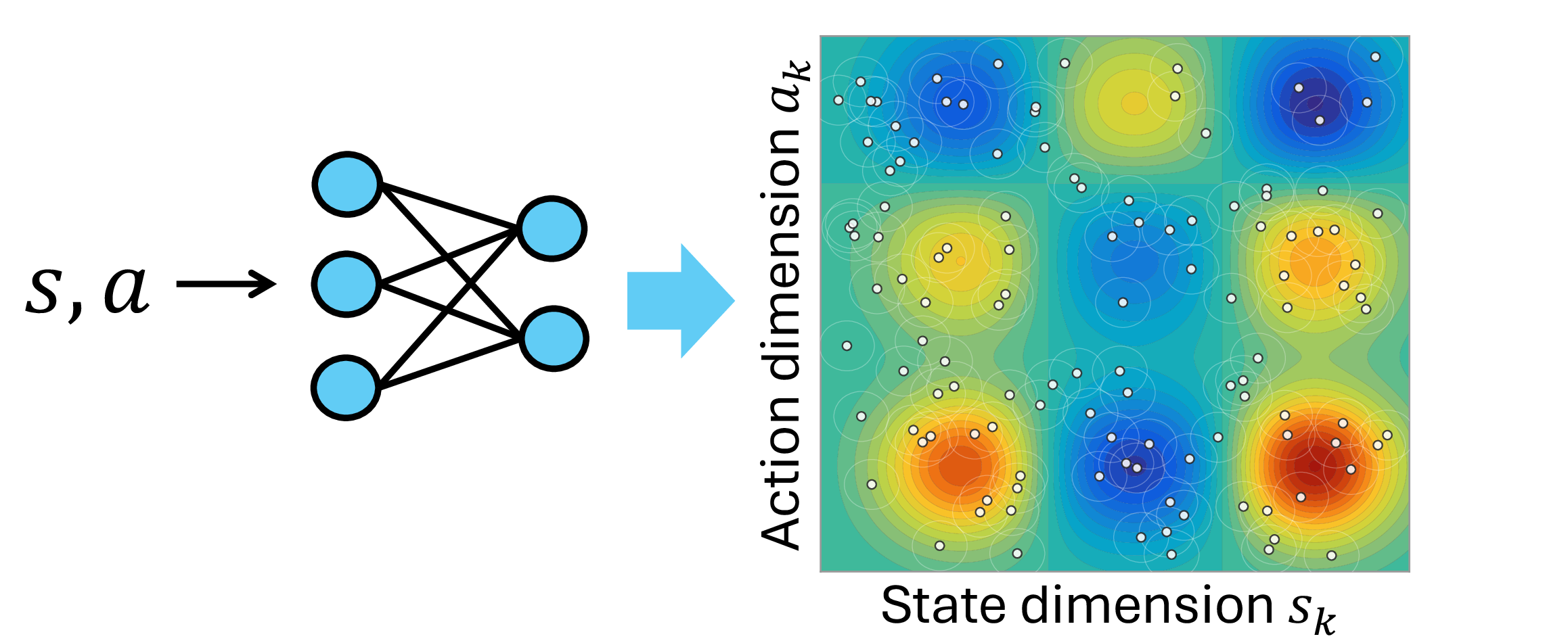
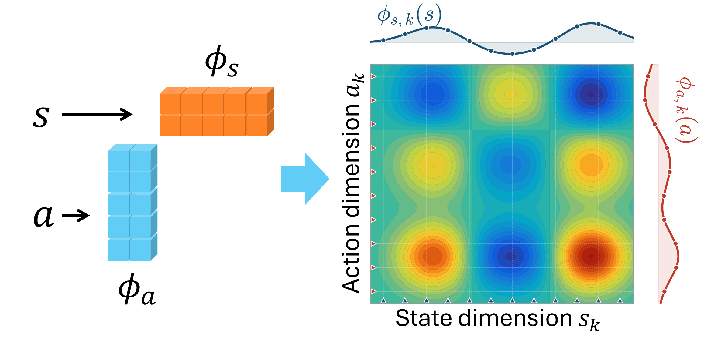
Figure 1: Comparison of representation structures. Factorization constrains the joint score landscape to the intersection of independent state and action profiles.. a — Joint Representation, b — Factorized Representation
In such cases, a joint representation must relearn shared state-side structure across actions, whereas a factored representation can reuse the same state-side modes while learning how actions modulate them.
To this end, we introduce Factored Spectral Representations (FaStR), which treats the transition kernel as a three-way tensor and learns one encoder per mode (state, action, next-state). Figure 1 illustrates the key difference. A joint encoder maps the concatenated pair \((s,a)\) directly into a state-action representation, so the learned score can vary freely over the full joint plane (Figure 1 (a)). In this view, local peaks in the score landscape may be tied to specific state-action regions. FaStR instead learns separate state and action profiles, and combines them through a Hadamard product (Figure 1 (b)). Thus, peaks and variations in the joint score must arise from the interaction of reusable state-side and action-side factors, encouraging sharing across rows and columns of the state-action plane. This structured sharing acts as an implicit regularizer and shifts the statistical burden from covering isolated state-action regions to estimating reusable factors, allowing the frozen feature to become useful for Bellman backups with fewer transitions when the dynamics match the factorization. Specifically, our contributions are as follows:
A factored view of spectral RL representations. We formulate the transition kernel as a three-mode object over state, action, and next state, and instantiate this view as a representation with a separate encoder for each of these three modes. The factored representation keeps these modes explicit while remaining compatible with contrastive training.
A representation-complexity separation under CP structure. We prove that the factored hypothesis class has a covering number that decomposes additively over the state, action, and next-state factors. Under CP realizability, this gives a sample-size gap implied by the bound; in the approximate case, the guarantee becomes a bias-estimation tradeoff.
Empirical evaluation and modular transfer. On DM Control Suite [11] tasks across morphologies and action dimensions, we test when the factored representation outperforms a joint state-action encoder. Gains grow with action dimension, but only when the factorization matches the dynamics. The same factorization also supports modular adaptation: under actuator shift, the state factor transfers intact and only the action factor is retrained.
2 Preliminaries↩︎
We consider a discounted MDP \(\mathcal{M}=(\mathcal{S},\mathcal{A},P,r,\gamma)\) with continuous state space \(\mathcal{S}\), continuous action space \(\mathcal{A}\), transition kernel \(P:\mathcal{S}\times\mathcal{A}\to\Delta(\mathcal{S})\), reward function \(r:\mathcal{S}\times\mathcal{A}\to\mathbb{R}\), and discount factor \(\gamma\in[0,1)\). The Q-function \(Q^\pi(s,a)=\mathbb{E}_\pi[\sum_{t=0}^\infty \gamma^t r(s_t,a_t)\mid s_0=s,a_0=a]\) satisfies the Bellman equation \[\label{eq:bellman-main} Q^\pi(s,a) = r(s,a) + \gamma \int_\mathcal{S} P(s'|s,a)\, V^\pi(s')\, ds',\tag{1}\] where \(V^\pi(s)=\mathbb{E}_{a\sim\pi(\cdot|s)}[Q^\pi(s,a)]\).
2.0.0.1 Linear MDPs and the linear-feature view.
A common simplification is to assume the transition kernel admits a finite-rank factorization. The linear MDP assumption [3] states that there exist a feature map \(\varphi:\mathcal{S}\times\mathcal{A}\to\mathbb{R}^d\), a kernel map \(\mu:\mathcal{S}\to\mathbb{R}^d\), and a reward parameter \(\theta_r\in\mathbb{R}^d\) such that \[\label{eq:linear-mdp} P(s'|s,a) = \varphi(s,a)^\top \mu(s'), \qquad r(s,a) = \varphi(s,a)^\top \theta_r.\tag{2}\] Under this assumption, the value function is linear in \(\varphi\): for any policy \(\pi\), \(Q^\pi(s,a)=\varphi(s,a)^\top w^\pi\) for some \(w^\pi\in\mathbb{R}^d\) that absorbs the integral against \(V^\pi\). The complexity of value learning then depends on the feature dimension \(d\) rather than the size of the state-action space, which enables provably efficient algorithms [3], [12]. In practice \(\varphi\) is unknown and must be learned from interaction data.
2.0.0.2 Spectral RL: learning transition-ratio scores.
Spectral representation methods learn \(\varphi\) and \(\mu\) from transition samples using self-supervised contrastive objectives [6], [8], [13], [14]. A scoring function \(h(s,a,s')=\varphi(s,a)^\top\mu(s')\) is trained to assign high values to true next-state samples \(s'\sim P(\cdot|s,a)\) and low values to negatives drawn from a reference distribution. At the population level, such objectives fit a transition-ratio score: the logit measures how plausible a candidate next state is under the transition kernel relative to the negative distribution. Existing deep spectral methods parameterize this score bilinearly, using a fused state-action feature on one side and a next-state feature on the other. The trained \(\varphi\) can then be used as the linear-MDP feature for downstream value learning.
The contrastive template that FaStR will instantiate is the ranking-based perturbed noise contrastive estimation (RP-NCE) objective [6], [8], in which negatives are obtained by perturbing true next states across a sequence of noise levels and the model is trained to rank a true (perturbed) positive above \(K-1\) corrupted alternatives: \[\label{eq:nce-prelim} \ell_{\text{NCE}} = -\frac{1}{MN}\sum_{m=1}^M\sum_{i=1}^N \log\frac{\exp\bigl(\varphi_i^\top \mu(\tilde{s}'_{i,0};\beta_m)\bigr)}{\sum_{j=0}^{K-1} \exp\bigl(\varphi_i^\top \mu(\tilde{s}'_{i,j};\beta_m)\bigr)},\tag{3}\] where \(\varphi_i=\varphi(s_i,a_i)\), \(\{\beta_m\}_{m=1}^M\) are noise levels along a variance-preserving (VP) schedule [15], which keeps the marginal variance fixed across levels, and \(\tilde{s}'_{i,j}\) denotes the \(j\)-th candidate next state corrupted at level \(\beta_m\), with \(j=0\) the true target and \(j\geq 1\) negatives drawn from other transitions in the mini-batch (in-batch negatives). At the population level this ranking objective is consistent with maximum likelihood estimation as the number of negatives grows [16]. Thus RP-NCE is best viewed as an estimator for a chosen transition-ratio score class; FaStR keeps this estimator but changes the score class from a fused bilinear to a mode-wise trilinear form.
2.0.0.3 The full spectral RL pipeline.
The contrastive loss is one component of the system. After training, the encoder \(\varphi\) is used as a frozen representation: a critic \(Q_\theta\) takes \(\varphi(s,a)\) as input and is trained by standard temporal-difference (TD) losses without back-propagating through \(\varphi\), and a policy network \(\pi\) is trained on top of this frozen representation. This separation between representation learning (the contrastive loss) and value learning (TD on the frozen feature) is what makes the learned \(\varphi\) usable as the linear-MDP feature in [3]. We work within this two-stage setup and locate our contribution in the structural form of the encoder \(\varphi\).
3 Method↩︎
3.1 The FaStR Framework↩︎
3.1.0.1 A tensor view of the transition kernel.
The standard linear MDP merges \(s\) and \(a\) into a single index and factorizes the resulting matrix \(P\in\mathbb{R}^{|\mathcal{S}\times\mathcal{A}|\times|\mathcal{S}|}\) via an SVD-like decomposition. This treats the two arguments uniformly, although the state specifies the configuration of the system while the action specifies the input applied to it. We separate the two arguments by viewing the transition kernel as a third-way tensor \(\mathcal{T}\in\mathbb{R}^{|\mathcal{S}|\times|\mathcal{A}|\times|\mathcal{S}|}\) indexed by \(s\), \(a\), and \(s'\).1
A standard general decomposition of such a tensor is the Tucker form [17], [18] \(P(s'|s,a)=\sum_{i,j,k}G_{ijk}\,\phi_{s,i}(s)\,\phi_{a,j}(a)\,m_k(s')\) with a core \(G\in\mathbb{R}^{d_s\times d_a\times d_m}\). The CP (CANDECOMP/PARAFAC) decomposition [18]–[20] is the special case where \(G\) is superdiagonal, \(G_{kkk}=1\), eliminating the core entirely; lower-rank or block-diagonal cores interpolate between CP and dense Tucker. Among these, FaStR uses the CP form; the case for this choice is made below in the context of contrastive training.
Assumption 1 (CP-Factored MDP). There exist feature maps \(\phi_s:\mathcal{S}\to\mathbb{R}^d\), \(\phi_a:\mathcal{A}\to\mathbb{R}^d\), a kernel map \(m:\mathcal{S}\to\mathbb{R}^d\), and a reward parameter \(\theta_r\in\mathbb{R}^d\) such that for all \((s,a,s')\): \[\begin{align} P(s'|s,a) &= \bigl(\phi_s(s)\odot\phi_a(a)\bigr)^\top m(s') = \sum_{k=1}^d \phi_{s,k}(s)\,\phi_{a,k}(a)\,m_k(s'), \tag{4}\\ r(s,a) &= \bigl(\phi_s(s)\odot\phi_a(a)\bigr)^\top \theta_r. \tag{5} \end{align}\] We write \(\psi(s,a):=\phi_s(s)\odot\phi_a(a)\in\mathbb{R}^d\) for the factored feature.
Each component \(k\) in Equation ref{eq:cp} is a rank-one term combining a state factor \(\phi_{s, k}(s)\), an action factor \(\phi_{a, k}(a)\), and a next-state factor \(m_k\left(s^{\prime}\right)\), with the action factor scaling the coupling between the other two. CP fits well when actions scale shared state-dependent modes of motion, such as posture or balance in locomotion; it underfits when strong contact or limb-coupling effects entangle modes across actions. The CP form has scale invariances between \(\phi_s\), \(\phi_a\), and \(m\), which are fixed by uniform norm bounds \(B_\phi\) and \(B_{m,\infty}\) throughout the analysis (Appendix 9.1); the implementation uses LayerNorm to stabilize the scales.
3.1.0.2 Factored representation and Q-linearity.
FaStR learns a feature that is useful for control, not only for predicting the next state. Let \(\psi(s,a):=\phi_s(s)\odot\phi_a(a)\). Under the CP-factored model, the transition and reward share this same feature: \(P(s'|s,a)=\psi(s,a)^\top m(s')\) and \(r(s,a)=\psi(s,a)^\top\theta_r\). Therefore, a Bellman backup does not leave the span of \(\psi\): for any policy \(\pi\), \(Q^\pi(s,a)\) is derived as: \[\label{eq:Q-linear} r(s,a)+\gamma\!\int_{\mathcal{S}}P(s'|s,a)V^\pi(s')ds' = \psi(s,a)^\top\!\left(\theta_r+\gamma\!\int_{\mathcal{S}}m(s')V^\pi(s')ds'\right) =: \psi(s,a)^\top w^\pi .\tag{6}\] Thus the downstream linear critic is not an additional assumption: once the transition and reward admit the CP form, the corresponding \(Q\)-function is linear in the learned factored feature. A derivation with norm bounds is given in Appendix 9.2.
3.1.0.3 Learning a trilinear transition-ratio score.
We learn the factors by viewing contrastive spectral learning as conditional ratio estimation. For an anchor \((s_i,a_i)\), the observed next state is the positive candidate and perturbed in-batch next states are negatives. InfoNCE [14] turns this into a classification problem: among one true next state and several distractors, the model is trained to assign the highest energy to the true candidate. At the population optimum, differences between these energies estimate the log ratio between the transition law at the anchor and the negative candidate distribution. RP-NCE repeats this classification across noise levels \(\beta\), giving a multi-scale ratio target for the next-state side. In standard spectral RL, this energy is bilinear: a fused state-action feature is matched with a \(\beta\)-conditioned next-state feature. FaStR instead chooses the CP trilinear energy \[f_\Theta(s,a,s';\beta) = \sum_{k=1}^d \phi_{s,\Theta,k}(s)\,\phi_{a,\Theta,k}(a)\, m_{\Theta,k}(s';\beta) = \bigl(\phi_{s,\Theta}(s)\odot\phi_{a,\Theta}(a)\bigr)^\top m_\Theta(s';\beta).\] Each coordinate is a ratio channel: the state factor selects a state-dependent mode, the action factor gates it, and the next-state factor scores the candidate at noise level \(\beta\). Substituting this energy into the RP-NCE template 3 gives \[\label{eq:nce} \ell_{\mathrm{FaStR}} = -\frac{1}{MN}\sum_{b=1}^{M}\sum_{i=1}^{N} \log \frac{ \exp\!\left(f_\Theta(s_i,a_i,\tilde{s}'_{i,0};\beta_b)\right)}{ \sum_{j=0}^{K-1} \exp\!\left(f_\Theta(s_i,a_i,\tilde{s}'_{i,j};\beta_b)\right) }.\tag{7}\] The learned state-action feature is the anchor side of this energy, \(\psi_\Theta(s,a)=\phi_{s,\Theta}(s)\odot\phi_{a,\Theta}(a)\). The downstream RFF critic then kernelizes the frozen \(\psi_\Theta\) for value learning, while the mode-wise geometry of \(\psi_\Theta\) is fixed by the transition-ratio energy. Together, the preceding pieces define the full FaStR pipeline: the CP factored MDP specifies the trilinear score class, Q-linearity explains why the anchor feature can support value learning, and RP-NCE provides the self-supervised signal that learns the factors from transitions. After this representation stage, we freeze \(\psi_\Theta\), train the actor and critic on top of it, and use the same downstream control pipeline as prior spectral RL; the structural change is in how transition data shape the state-action feature. Algorithm 4 gives the per-step update.
3.1.0.4 CP vs. Tucker cores.
The CP form is the diagonal member of a broader trilinear transition-ratio score class, written as \(h(s,a,s')=\phi_s(s)^\top M(s')\phi_a(a)\), with \(M(s')\) generated by the next-state mode and restricted to be diagonal under CP. Other parameterizations correspond to less constrained interaction matrices: a dense \(d_s\times d_a\) matrix gives full Tucker, and intermediate cases (low-rank \(M(s')=U(s')V(s')^\top\), block-diagonal cores) interpolate between CP and dense Tucker. Such factorizations have been used in prior bilinear MDP methods trained with regression or maximum-likelihood objectives [4], [21], [22], where the gradient on \(M(s')\) is full-rank per anchor and large interaction matrices can be trained with enough data.
Under contrastive training the gradient structure is different. The chain rule on \(h_{ij}=\phi_s(s_i)^\top M(s'_j)\phi_a(a_i)\) gives \[\label{eq:rank-one-grad} \nabla_{\mathrm{vec}(M(s'_j))}\,\ell_{\text{NCE}} \;\in\; \mathrm{span}\bigl\{\phi_a(a_i)\otimes\phi_s(s_i)\bigr\},\tag{8}\] a one-dimensional subspace per anchor. A mini-batch of \(N\) anchors therefore covers at most \(\min(N,\dim(M))\) directions in the parameter space of \(M(s')\) in a single update. This rank-one structure follows from the conditional bilinear form of the trilinear score and is the same for any parameterization of \(M\): low-rank or block-diagonal cores reduce the parameter count below \(d_s d_a\), but each anchor still contributes a rank-one direction projected onto the corresponding submanifold. For dense Tucker, \(\dim(M)=d_s d_a\), so per-batch coverage requires \(N\geq d_s d_a\), which scales quadratically in the per-mode dimension and exceeds typical batch sizes. The CP form has \(\dim(M)=d\), so the linear requirement \(N\geq d\) is met by standard mini-batch sizes.
Whether structured cores can accumulate the full parameter space across many SGD updates at realistic compute is an empirical question. The underlying issue is that any structured-core fix faces a three-way constraint: encoder capacity, NCE validity (the negative count must reach the effective NCE dimension, here \(N\geq d_s d_a\), for the contrastive logit to be non-degenerate), and per-batch gradient coverage cannot be satisfied simultaneously at standard batch sizes. Reducing \(d_s, d_a\) to satisfy validity makes encoder capacity the binding constraint and removes the representational benefit. Appendix 10.1 reports a controlled three-way encoder ablation (monolithic, concat-of-separate, Tucker) and a separate capacity test, showing that no choice of Tucker rank within this constraint matches CP under matched compute.
3.2 Provable Representation Efficiency↩︎
Section 3.1 chose CP among bilinear parameterizations on training-dynamics grounds. The matching statistical question is whether CP also makes the representation class easier to learn from a finite sample. We answer it in three steps. We first bound the size of the factored class relative to the joint class (Theorem 1). We then convert this bound into a finite-sample bound on representation error (Proposition 2). Finally, we invert the bound to compare the sample sizes that suffice for each class to reach a target error (Proposition 3). The dimension dependence of the final result matches the empirical pattern in Section 4.
We work with two scoring classes. The factored class \(\mathcal{G}_{\text{fac}}\) contains \(g(s,a,s')=(\phi_s(s)\odot\phi_a(a))^\top m(s')\) with \((\phi_s,\phi_a,m)\in\mathcal{F}_s\times\mathcal{F}_a\times\mathcal{F}_m\); the joint class \(\mathcal{G}_{\text{joint}}\) contains \(g(s,a,s')=\varphi(s,a)^\top\mu(s')\) with \(\varphi\in\mathcal{F}_{sa}\), \(\mu\in\mathcal{F}_m\). Norm bounds and the convention for sup-\(\ell_2\) covering numbers are in Appendix 9.1.
3.2.0.1 Step 1: bounding the size of the factored class.
A monolithic encoder takes each \((s,a)\) pair as a single input, and the size of its hypothesis class scales with the combined state-action dimension. The CP parameterization splits the score into three networks: a state factor, an action factor, and a kernel encoder, coupled through a diagonal trilinear interaction (the Hadamard form of Eq. 4 ). The size of the resulting class is then controlled by the three component networks separately rather than by their product. Covering numbers, a standard measure of the size of a function class, make this precise.
Theorem 1 (Covering-number decomposition). For every \(\epsilon>0\), \[\log\mathcal{N}(\mathcal{G}_{\emph{fac}},\epsilon) \;\le\; \log\mathcal{N}\!\left(\mathcal{F}_s,\tfrac{\epsilon}{3B_{m,\infty}B_\phi}\right) + \log\mathcal{N}\!\left(\mathcal{F}_a,\tfrac{\epsilon}{3B_{m,\infty}B_\phi}\right) + \log\mathcal{N}\!\left(\mathcal{F}_m,\tfrac{\epsilon}{3B_\phi^2}\right).\] If \(\mathcal{F}_{sa}\) contains every Hadamard product \(\phi_s\odot\phi_a\) with \((\phi_s,\phi_a)\in\mathcal{F}_s\times\mathcal{F}_a\), then \(\mathcal{G}_{\emph{fac}}\subseteq\mathcal{G}_{\emph{joint}}\), and the inclusion holds for both covering numbers and Rademacher complexities at every sample size.
Proof. See Appendix 9.3. ◻
For Lipschitz encoders on compact domains, this gives an exponent \(D_{\max}=\max(d_s,d_a)\) for the factored class versus \(D_{\mathrm{sum}}=d_s+d_a\) for the joint class, leaving a gap of \(\min(d_s,d_a)\) in the rate exponent that is formalized as a sample-size separation in Proposition 3.
3.2.0.2 What the bound says in operational terms.
In sample-size terms, the covering number is the number of transitions needed for the contrastive loss to separate two encoder triples within a target tolerance. A smaller covering number means the empirical loss is close to its population value at smaller \(n\), so the resulting \(\psi=\phi_s\odot\phi_a\) is available as a TD feature at smaller \(n\). Take humanoid as a concrete case. The state has \(d_s=67\) proprioceptive coordinates, the action has \(d_a=21\) actuator commands, and the standard approach fits the transition density on the joint \(88\)-dimensional input. The CP form fits two smaller pieces instead: a \(67\)-dimensional state feature, and \(21\) per-actuator gains that say how each actuator scales that feature. Theorem 1 states this same split at the level of the covering number. Proposition 2 turns the smaller class size into a smaller representation error at fixed \(n\). Proposition 3 inverts the bound and gives the smaller sample size needed for a target error. Once \(\psi\) is frozen, TD on \(\psi\) satisfies the linear-MDP sample-complexity guarantees of [3], so a smaller representation error at a given \(n\) becomes a smaller return gap in policy learning.
3.2.0.3 Step 2: from class size to representation error.
A smaller class size matters only if it leads to a smaller generalization gap. The target we analyze is the \(L_2\) representation objective of [7], the squared \(L^2(\nu)\) distance from the true transition density, \[L(g) := \mathbb{E}_\rho\!\left[\int_\mathcal{S}\bigl(P(s'\mid s,a)-g(s,a,s')\bigr)^2 d\nu(s')\right].\] We analyze this objective rather than NCE itself because finite-sample guarantees are tractable for the \(L_2\) surrogate at the population level, while the contrastive loss serves as its practical proxy at training time [7].
Proposition 2 (Finite-sample generalization). Let \(\mathcal{G}\in\{\mathcal{G}_{\emph{fac}},\mathcal{G}_{\emph{joint}}\}\) with \(|g|\le B_g\), and let \(\hat{g}_n\) be an empirical minimizer of the centered objective on \(n\) i.i.d.transitions. With probability at least \(1-\delta\), \[L(\hat{g}_n) \;\le\; \underbrace{L(g^*_\mathcal{G})}_{\text{approximation}} \;+\; \underbrace{8\,\mathcal{R}_n(\mathcal{G}) + 4\,\mathcal{R}_n(\mathcal{H}_\mathcal{G})}_{\text{estimation}} \;+\; O\!\left((B_g+B_g^2)\sqrt{\tfrac{\log(1/\delta)}{n}}\right),\] where \(\mathcal{H}_\mathcal{G}:=\{(s,a)\mapsto\int g^2(s,a,u)\,d\nu(u):g\in\mathcal{G}\}\) is the integrated quadratic class arising from expanding the squared loss. The quadratic class satisfies \(\mathcal{N}(\mathcal{H}_\mathcal{G},\epsilon)\le\mathcal{N}(\mathcal{G},\epsilon/(2B_g))\), so its Rademacher complexity inherits the rate of \(\mathcal{G}\) itself.
Proof. See Appendix 9.6. ◻
The bound has two terms with opposite scaling. The approximation term \(L(g^*_\mathcal{G})\) measures whether the class contains the true dynamics; under exact CP realizability and the inclusion of Theorem 1, both classes contain the truth and this term is zero for both. Under approximate CP, the factored class has an irreducible bias \(\epsilon_{\mathrm{CP}}^2:=\inf_{g\in\mathcal{G}_{\text{fac}}}L(g)\) that the joint class does not have. The estimation term is smaller for the factored class: both Rademacher terms inherit the smaller exponent \(D_{\max}\) from Theorem 1, so the factored class converges faster in \(n\).
3.2.0.4 Step 3: from representation error to sample size.
The previous two steps bound representation error at a fixed sample size. The inverse question is how many samples each class needs to reach the same target error.
Proposition 3 (Sufficient-sample-size separation). Assume exact CP realizability, the inclusion condition of Theorem 1, and \(L\)-Lipschitz encoder classes on compact domains with \(D_{\max}\geq 3\). Proposition 2 then gives certificates of the form \(L(\hat{g}_n^{\mathrm{fac}})\le C_{\mathrm{fac}}(\delta)\,n^{-1/D_{\max}}\) and \(L(\hat{g}_n^{\mathrm{joint}})\le C_{\mathrm{joint}}(\delta)\,n^{-1/D_{\mathrm{sum}}}\), with \(C_{\mathrm{fac}}, C_{\mathrm{joint}}\) depending polynomially on the norm bounds, Lipschitz constants, and feature dimension, and logarithmically on \(1/\delta\). Let \(n_{\mathrm{fac}}^{\mathrm{suff}}(\epsilon)\) and \(n_{\mathrm{joint}}^{\mathrm{suff}}(\epsilon)\) be the smallest \(n\) at which each certificate guarantees error at most \(\epsilon^2\). Then \[\frac{n_{\mathrm{joint}}^{\mathrm{suff}}(\epsilon)}{n_{\mathrm{fac}}^{\mathrm{suff}}(\epsilon)} \;=\;\Theta\!\left(\epsilon^{-2\min(d_s,d_a)}\right) \quad \text{as } \epsilon\to 0.\]
Proof. See Appendix 9.7. ◻
The factored class therefore has a smaller certified sample requirement, with the exponent gap equal to \(\min(d_s,d_a)\). This gap is meaningful when the smaller of the state and action dimensions is nontrivial and the CP bias is small; otherwise the approximate-CP certificate \(L(\hat{g}_n^{\mathrm{fac}}) \lesssim \epsilon_{\mathrm{CP}}^2 + C_{\mathrm{fac}}(\delta)n^{-1/D_{\max}}\) can be dominated by bias. We test these two conditions in Section 4 and Appendix 10.2. Appendix 9.8 further gives a conditional LSVI-UCB implication: if the learned feature satisfies approximate Bellman linearity, the factored structure can reduce the representation cost of obtaining features suitable for optimism-driven exploration.
4 Experiments↩︎
The experiments evaluate FaStR on two axes. First, on standard locomotion benchmarks whose morphology is well aligned with a CP-style factorization, we compare FaStR against the monolithic encoder under an otherwise identical pipeline (Section 4.2). Second, in a transfer setting where only the action-to-torque mapping changes between training and adaptation, we test whether the separable state factor enables sample-efficient adaptation that a joint encoder cannot support (Section [sec:exp-transfer]).
4.1 Setup↩︎
We evaluate on DM Control Suite [11] locomotion tasks that vary in action dimensionality and morphology, with \(\dim(\mathcal{A})\in\{6,12,21,38\}\) and shared proprioceptive observations. To attribute performance differences to the encoder structure alone, we use a controlled protocol: FaStR and the monolithic baseline (CTRL-SR [6]) share identical total parameter counts, hidden dimensions, learning rates, noise schedules, and training budgets, with no task-specific tuning for either method. The only varying component is the representation: FaStR’s factored encoders \((\phi_s,\phi_a,m)\) versus CTRL-SR’s joint encoder \(\varphi([s;a])\). Main-text learning curves (Figure 2) compare FaStR against CTRL-SR. Table 1 additionally reports final-return comparisons against Diff-SR [9], a second spectral RL baseline that replaces the contrastive objective with a diffusion next-state model on the same TD3 backbone, and against TD7 [23] and SAC [2], the current model-free SOTA. SAC and TD7 use the architectures and hyperparameters from the original papers. We report two SAC variants, SAC(3-layer) and SAC(2-layer), both wider per layer than the spectral methods’ actor, so a capacity mismatch is not the source of the gap. We compare only against model-free baselines; model-based methods on this suite were evaluated by [6] and gave lower returns than the spectral RL baselines. Full hyperparameters are in Appendix 8.
4.2 Sample Efficiency on Locomotion Benchmarks↩︎
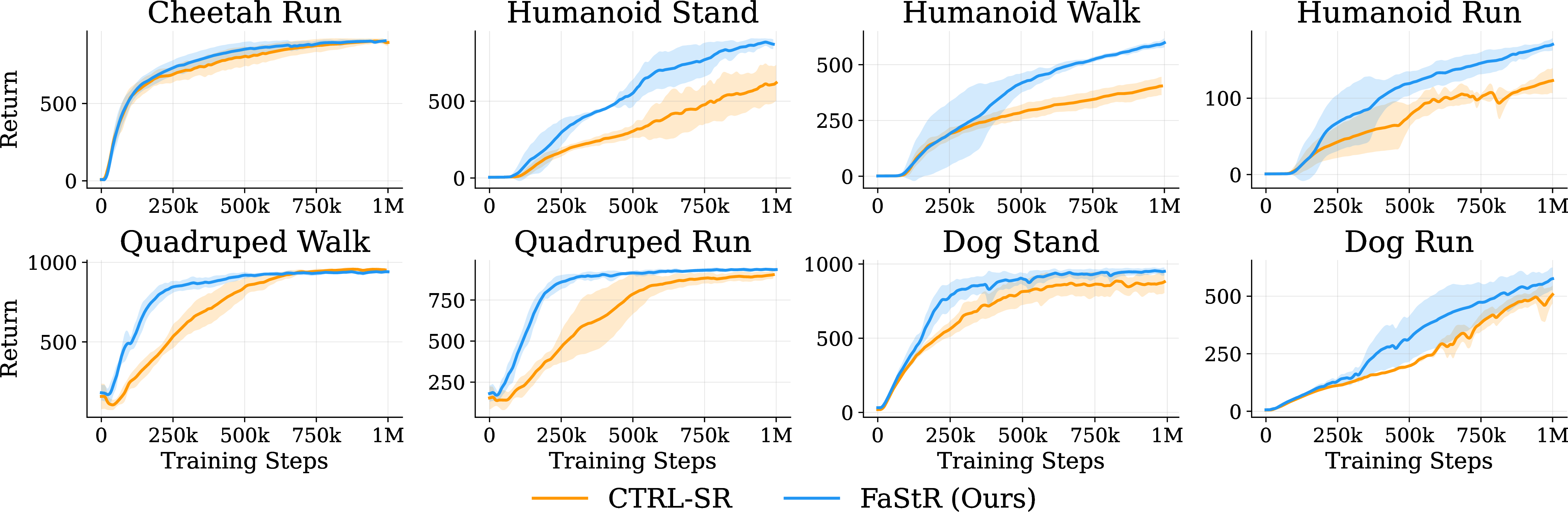
On the Humanoid tasks, where torso-limb morphology admits a CP factorization (independent joint groups scaling shared postural modes), FaStR gives higher returns than the controlled baseline by margins above seed-level noise across all three tasks, attributing the difference to the representation. On the Dog environment, the larger action dimension is partly offset by stronger ground-contact dynamics that introduce state-action coupling, giving improvements with wider variance. The same ordering holds against Diff-SR on all five high-action-dim tasks (Table 1), so the gain is not specific to the contrastive objective.
On the Quadruped tasks, FaStR converges to CTRL-SR’s terminal performance with higher sample efficiency: on Quadruped-Run, it reaches the baseline’s converged level earlier in training and exceeds it asymptotically; on Quadruped-Walk, the final return is slightly below the baseline, but FaStR reaches near-converged performance earlier than CTRL-SR at any fixed performance threshold. The improvement on this family appears as faster convergence rather than a higher asymptote, which is consistent with the bias-estimation interpretation: the estimation advantage appears in the rate at which the representation becomes usable for value learning. On Cheetah-Run, Walker-Walk, and Walker-Run (\(\dim\mathcal{A}{\le}6\)), FaStR matches the baselines without significant gain, the regime predicted by Proposition 3 in which small \(\min(d_s,d_a)\) gives a small estimation advantage in the certificate.
| \(\dim\Acal=6\) | \(\dim\Acal=12\) | \(\dim\Acal=21\) | \(\dim\Acal=38\) | |||||||
|---|---|---|---|---|---|---|---|---|---|---|
| 2-4 (lr)5-6 (lr)7-9 (lr)10-11 | Cheetah Run | Walker Walk | Walker Run | Quad.Walk | Quad.Run | Hum.Stand | Hum.Walk | Hum.Run | Dog Stand | Dog Run |
| SAC(2-layer) | \(660\pm9\) | \(880\pm5\) | \(650\pm19\) | \(880\pm6\) | \(797\pm18\) | \(200\pm70\) | \(143\pm99\) | \(\;\,60\pm27\) | \(500\pm9\) | \(\;\,44\pm48\) |
| SAC(3-layer) | \(901\pm5\) | \(972\pm3\) | \(802\pm7\) | \(946\pm13\) | \(931\pm9\) | \(446\pm52\) | \(214\pm154\) | \(\;\,87\pm33\) | \(577\pm11\) | \(\;\,67\pm34\) |
| TD7 | \(898\pm1\) | \(\mathbf{979\pm1}\) | \(815\pm18\) | \(952\pm3\) | \(921\pm20\) | \(728\pm176\) | \(365\pm216\) | \(\;\,85\pm49\) | \(891\pm21\) | \(192\pm12\) |
| Diff-SR | \(\mathbf{910\pm4}\) | \(978\pm2\) | \(\mathbf{827\pm10}\) | \(953\pm5\) | \(903\pm27\) | \(663\pm101\) | \(358\pm18\) | \(111\pm18\) | \(913\pm22\) | \(302\pm81\) |
| CTRL-SR | \(900\pm15\) | \(978\pm1\) | \(809\pm29\) | \(\mathbf{955\pm9}\) | \(900\pm24\) | \(607\pm122\) | \(399\pm40\) | \(120\pm15\) | \(870\pm70\) | \(499\pm45\) |
| FaStR (Ours) | \(903\pm8\) | \(974\pm3\) | \(809\pm17\) | \(949\pm9\) | \(\mathbf{936\pm9}\) | \(\mathbf{877\pm28}\) | \(\mathbf{591\pm15}\) | \(\mathbf{168\pm7}\) | \(\mathbf{951\pm24}\) | \(\mathbf{560\pm50}\) |
2pt
2.5pt
4.2.0.1 Mechanism check.
Appendix 10.1 runs a controlled three-way ablation that isolates the CP interaction from encoder separation and from generic multiplicative coupling. A concat-of-separate variant, with independent encoders feeding a joint MLP, gives only a small improvement over the monolithic baseline, well below FaStR’s gain. A full Tucker-core variant has the rank-deficient gradient issue of Section 3.1, and a separate capacity test rules out the low-rank workaround. The CP interaction is therefore the source of the gain. The offline CP-misfit diagnostic (Appendix 10.2) further shows that gains track structural alignment with the dynamics, not action dimension alone.
4.3 Modular Reuse of \(\phi_s\) under Actuator Shift↩︎
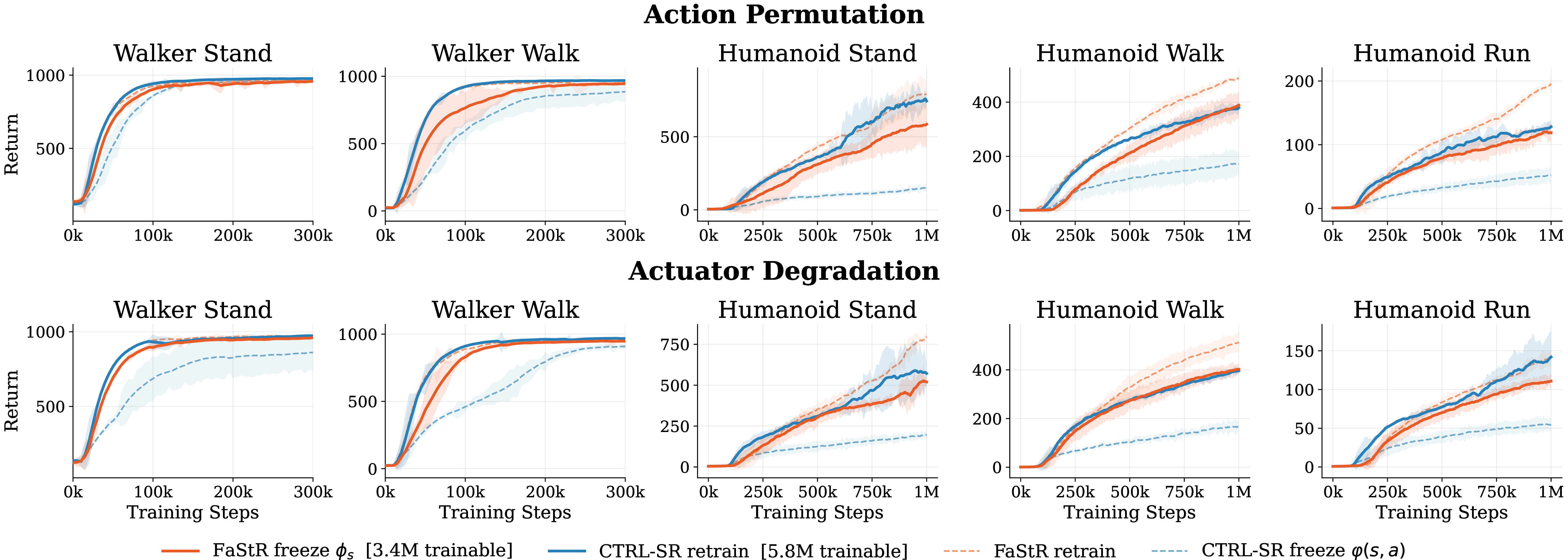
We test transfer in a setting where the physical dynamics of the system are unchanged but the action-to-torque interface is rewritten. The CP factorization predicts what each architecture preserves under such a change. Under FaStR, \(\phi_s\) depends only on the state-side dynamics of the body and should remain valid when only the action-to-torque map shifts; under a joint encoder, state and action are coupled through every parameter, so any change to the interface leaks throughout the encoder and no component is guaranteed to remain valid. The factored representation therefore admits an option a joint encoder does not: keep \(\phi_s\), adapt only \(\phi_a\).
We instantiate two such rewrites. Actuator degradation applies independent per-joint gain scaling and polarity inversion. Action permutation randomly reassigns joint channel indices. Together they capture the basic ways an action interface can drift, independent scaling and reordering, and serve as a basic simulation of the transfer problem without the confounding factors of full domain shift. The transition over true torques and the reward are both unchanged; only the path from policy output to actuation is rewritten. Source and target therefore share the same task, reward, and body, and differ only in the actuator interface, so any retraining cost reflects what the representation failed to preserve. For each architecture we freeze the largest state-dependent component (\(\phi_s\) for FaStR, the joint encoder \(\varphi\) for CTRL-SR) and reinitialize everything downstream. Walker is a parity check on matched pre-shift returns; Humanoid is the diagnostic.
4.3.0.1 What is preserved, and at what cost.
On a CP-factored MDP, which component to keep across an actuator shift is determined by the representation, not a hyperparameter the practitioner has to choose. A monolithic encoder gives no such handle: the only options are to retrain everything or to freeze arbitrary subsets, neither of which uses structural information about the shift. A second concern is whether the frozen component is a worse starting point than learning from scratch, which would limit FaStR freeze to a lower final return than CTRL-SR scratch. The Humanoid match in Figure 3 excludes this: the parameters that CTRL-SR retrains from scratch are the same ones FaStR keeps unchanged, reusing them matches CTRL-SR-scratch on the target task (Humanoid-Walk: 393.7 vs. under permutation, 401.8 vs. under degradation). The modularity is therefore useful in practice and not only as a structural property.
5 Related Work↩︎
Modern spectral RL methods learn policy-agnostic features with self-supervised objectives that decompose the transition kernel: SPEDER [7] uses orthogonality-regularized spectral contrastive learning, CTRL-SR [6], [8] uses ranking-based perturbed NCE, Diff-SR [9] handles multimodal next states with a diffusion objective, and the Spectral Bellman Method [10] uses a Bellman-aligned principle. FaStR is orthogonal to this objective-level progress: it retains the NCE pipeline but replaces the fused encoder with a CP-factored one, moving factored structure from the objective into the representation itself. This also separates FaStR from prior uses of multiplicative coupling through FiLM [24], hypernetworks [25], or temporal InfoNCE (a mutual-information contrastive loss) with split encoders [26], which do not factorize the transition kernel itself. Low-rank MDPs [3]–[5] and related exploration, representation, and matrix-completion analyses [12], [27]–[30] also impose structure on transitions, but treat the joint state-action feature as a single function. Other tensor or factored RL methods place structure on the Q-table, continuous-action value function, or multi-agent Q-tensor [31]–[34]. FaStR sits between these lines by placing factored structure on the transition kernel within a deep spectral representation-learning framework.
6 Discussion and Conclusion↩︎
We introduce FaStR, a spectral representation learning framework that decomposes the transition kernel as a three-way tensor with state, action, and next-state factors, estimated through a trilinear structured contrastive objective. The resulting factored class has a quantifiable statistical advantage: transition samples constrain reusable state and action factors rather than isolated state-action pairs, so the frozen feature can become useful for Bellman backups earlier in training when the CP structure matches the dynamics. The same separation also supports modular adaptation: when the action-to-torque mapping shifts, the state factor transfers intact while only the action factor needs to be retrained. The broader principle is that representations should structurally mirror the physical factorization of future embodied systems into sensors, actuators, and the dynamics connecting them.
7 Limitations.↩︎
The CP form \(\phi_s(s)\odot\phi_a(a)\) treats the state and the action as two atomic axes. Environments with strongly coupled joints and tight state–action interdependence, such as Ant-style locomotion, fall outside the regime this two-way split captures cleanly, since the encoder is forced to absorb all sub-axis interactions internally. A hierarchical factorization over actuator or body-part groups, e.g.\(\phi_s(s)=\phi_{\text{torso}}\odot\phi_{\text{limbs}}\) or a tree-shaped CP, fits inside the same framework and is a clean next step.Second, Diagonal \(M\) corresponds to CP rank one along the next-state axis. A low-rank Tucker core \(G\in\mathbb{R}^{d\times d}\) recovers more interaction terms but enlarges the effective NCE dimension from \(d\) to \(d^2\), reintroducing the constraint that motivated the diagonal choice. Mapping the rank–capacity trade-off, e.g.via low-rank rather than diagonal \(M\), would close the gap between the CP and Tucker ends of this spectrum. Also, all experiments are conducted in the DMControl proprioceptive locomotion suite. Pixel-input variants and physical-robot deployment are not evaluated; the latter introduces sensor noise, latency, and actuator drift that the actuator-shift experiments only partially approximate.
8 Implementation Details↩︎
This appendix specifies the full training and evaluation protocol used in Section 4, together with the architectural and optimization hyperparameters of FaStR and the five baselines reported in Table 1: CTRL-SR [6], Diff-SR [9], SAC [2] in two width-depth variants (3-layer and 2-layer), and TD7 [23]. Hyperparameters that are common across methods (environment configuration, replay, evaluation cadence, total interaction budget) are listed once in Section 8.1; method-specific settings are listed in Sections 8.2–8.6 and summarized side-by-side in Table 2. We follow the convention of reporting every hyperparameter that was set in our runs, including those left at the original authors’ defaults, so that the protocol is self-contained.
8.1 Shared Training Protocol↩︎
All experiments use the DeepMind Control Suite [11] with proprioceptive observations, action repeat (frame skip) of 2, and episode length 1000 environment steps. We train each agent for \(1{\times}10^6\) environment frames (i.e.\(5{\times}10^5\) agent steps after action repeat) per task. Each agent maintains a single uniform-sampling replay buffer of capacity \(1{\times}10^6\) transitions, with the first \(10{,}000\) frames collected by a uniform random policy as a warm start before any gradient update. Evaluation is performed every \(10{,}000\) environment frames by rolling out the deterministic actor (for TD3-based methods: TD3 mean action; for SAC: tanh-Gaussian mean) for \(10\) episodes; we report the mean undiscounted return over the last 10 evaluation checkpoints, averaged over \(5\) random seeds, with shaded bands or \(\pm1\) standard deviations across seeds. Observation normalization (running mean and standard deviation) is enabled for the spectral methods (FaStR and CTRL-SR), following [6], and disabled for the SAC and TD7 baselines, matching their original implementations. All methods use the discount factor \(\gamma{=}0.99\), the same set of seeds \(\{0,1,2,3,42\}\), and a single update per environment step (update-to-data ratio 1).
8.2 FaStR (Ours)↩︎
8.2.0.1 Architecture.
All encoders, the noise schedule, and design defaults that are not explicitly varied below follow [6]. Encoders are ResidualMLPs with LayerNorm, ELU activations, and Mish activations inside the contrastive head. The state factor \(\phi_s\) maps \(\dim(\mathcal{S})\to 512\to 512\to d\); the action factor \(\phi_a\) maps \(\dim(\mathcal{A})\to 512\to 512\to d\); the kernel encoder \(m\) maps \(\dim(\mathcal{S})+128\to 512\to 512\to d\), where the additional 128 dimensions encode the perturbation level via a sinusoidal time embedding. We set \(d{=}512\) throughout. The factored feature \(\psi(s,a)=\phi_s(s)\odot\phi_a(a)\) is fed to a twin Q critic consisting of a random Fourier features (RFF) [35] projection of width \(1024\) followed by a 2-layer MLP head \([512]\) with LayerNorm and ELU; this critic is architecturally identical to the CTRL-SR critic so that the only varying component is the encoder. The actor is a deterministic policy network with hidden sizes \([512,512,512]\), ELU activations, and a final \(\tanh\) that maps to \([-1,1]^{\dim(\mathcal{A})}\).
8.2.0.2 Optimization.
All four networks (state factor, action factor, kernel encoder, critic) are trained with Adam (default \((\beta_1,\beta_2)=(0.9,0.999)\), no weight decay). Critic and actor learning rates are \(3{\times}10^{-4}\); the representation learning rate (jointly applied to \(\phi_s,\phi_a,m\)) is \(1{\times}10^{-4}\). Polyak averaging (i.e., \(\bar\theta\leftarrow(1-\tau)\bar\theta+\tau\theta\)) with \(\tau{=}0.005\) is used for both the critic and the representation targets; actor and critic updates are performed every environment
step (actor_update_freq=1). The mini-batch size is \(N{=}512\), matching the negative-sample count \(K{=}N{=}512\) implicit in the in-batch RP-NCE objective. Exploration uses
Gaussian action noise \(\mathcal{N}(0,\sigma{=}0.2)\) clipped to \([-1,1]^{\dim(\mathcal{A})}\); target action smoothing uses \(\mathcal{N}(0,\tilde{\sigma{=}}0.2)\) clipped to \([-0.3,0.3]\). Gradients of the critic loss are not back-propagated through the representation (back_critic_grad=false). One
training step is summarized in Algorithm 4.
8.2.0.3 Representation objective.
We use the ranking-based perturbed NCE loss 7 to train the trilinear transition-ratio score, with \(M{=}25\) noise levels on a variance-preserving (VP) schedule. The ranking variant is enabled
(ranking=true), and the auxiliary bilinear-MDP regression term of [6] is kept at its default weight \(\beta{=}1.0\). The combined training loss is \(\ell_{\mathrm{FaStR}} + \lambda_r\,\ell_{\mathrm{reward}} + \lambda_Q\,\ell_{\mathrm{critic}}\) with \(\lambda_{\mathrm{ctrl}}{=}\lambda_r{=}\lambda_Q{=}1.0\); the reward head is a 2-layer MLP \([512]\) on top of \(\psi\), identical in structure to the CTRL-SR
reward head.

8.3 CTRL-SR↩︎
CTRL-SR [6] serves as the most controlled baseline: the only architectural difference from FaStR is that the transition-ratio logit uses a single monolithic encoder \(\varphi:\mathcal{S}\times\mathcal{A}\to\mathbb{R}^d\) taking the concatenation \([s;a]\) as input, rather than a CP trilinear score built from separate state and action factors. The encoder \(\varphi\) is a 2-layer ResidualMLP \([\dim(\mathcal{S})+\dim(\mathcal{A})] \to 512 \to 512 \to d\) with \(d{=}512\), LayerNorm, and ELU activations; the kernel encoder \(m\), RFF-MLP critic, deterministic actor \([512,512,512]\), reward head, optimizer (Adam), learning rates (\(3{\times}10^{-4}\) for actor/critic and \(1{\times}10^{-4}\) for representation), Polyak factor \(\tau{=}0.005\), target/exploration action noise, batch size \(N{=}512\), RP-NCE noise levels \(M{=}25\), ranking objective, and update cadence are all identical to those of FaStR. We use the authors’ open-source implementation without modification.
8.4 Diff-SR↩︎
Diff-SR [9] is the second spectral RL baseline. It uses the same TD3 actor and critic backbone as CTRL-SR and FaStR, but replaces the ranking-based perturbed NCE objective with a denoising-diffusion next-state model: the joint encoder \(\phi:\mathcal{S}\times\mathcal{A}\to\mathbb{R}^d\) and the kernel encoder \(\mu:\mathcal{S}\times[1,T]\to\mathbb{R}^{d\times\dim(\mathcal{S})}\) are trained by score matching against the variance-preserving (VP) noise schedule of [9], with the predicted noise factorized as \(\hat{\epsilon}(s,a,s'_t,t)=\phi(s,a)^\top\mu(s'_t,t)\). The state and action inputs to \(\phi\) are first projected by 2-layer Mish MLPs of widths \([256,128]\) to a shared embedding dimension of \(128\) each, concatenated to a \(256\)-dim vector, and passed to a 3-layer ResidualMLP \(256\to512\to512\to512\to d\) with \(d{=}512\). The kernel encoder \(\mu\) takes \((s'_t,t)\) as input, where \(t\) is encoded by a sinusoidal positional embedding of width \(128\) followed by a 2-layer Mish MLP, and outputs a \(d\times\dim(\mathcal{S})\) matrix via a 3-layer ResidualMLP \([\dim(\mathcal{S})+128]\to 512\to 512\to 512\to d\cdot\dim(\mathcal{S})\). The diffusion uses \(T{=}50\) sample steps with the noisy state clamped to \([-10,10]\). The critic is the same RFF-MLP twin Q as CTRL-SR (RFF projection of width \(1024\) followed by a 1-hidden-layer \([512]\) head); the deterministic actor is a \([512,512,512]\) MLP with LayerNorm and a final \(\tanh\); the reward head is an RFF-MLP with the same shape as the critic head.
All four networks are trained with Adam. Critic and actor learning rates are \(3{\times}10^{-4}\); the representation learning rate (jointly applied to \(\phi,\mu\), and the reward head)
is \(1{\times}10^{-4}\). Polyak averaging uses \(\tau{=}0.005\), and actor and critic updates are performed every environment step (actor_update_freq=1,
feature_update_ratio=1). Mini-batch size is \(N{=}512\), matching the spectral baselines. Exploration uses Gaussian noise \(\mathcal{N}(0,\sigma{=}0.2)\) clipped to \([-1,1]^{\dim(\mathcal{A})}\); target action smoothing uses \(\mathcal{N}(0,\tilde{\sigma{=}}0.2)\) clipped to \([-0.3,0.3]\). The combined training loss is \(\lambda_{\mathrm{diff}}\,\ell_{\mathrm{diffusion}} + \lambda_r\,\ell_{\mathrm{reward}} + \lambda_Q\,\ell_{\mathrm{critic}}\) with \(\lambda_{\mathrm{diff}}{=}1.0\), \(\lambda_r{=}0.1\), and \(\lambda_Q{=}1.0\); gradients of the critic loss are not back-propagated through the representation (back_critic_grad=false). Observation normalization is
enabled, matching CTRL-SR and FaStR. We use the open-source implementation accompanying [9] without modification.
8.5 SAC↩︎
SAC [2] uses a stochastic tanh-Gaussian policy and a twin Q critic with ELU activations and LayerNorm. The critic takes the raw \((s,a)\) concatenation as input; no representation learning is performed. We report two width-depth variants. SAC(3-layer) uses hidden sizes \([1024,1024,1024]\) for both the actor and the
critic, matching the standard SAC configuration on DM Control Suite. SAC(2-layer) uses hidden sizes \([1024,1024]\) for both, isolating the effect of removing one hidden layer at the same per-layer width. All other settings
are shared between the two variants. Following [2], the entropy coefficient \(\alpha\) is learned online
(automatic entropy tuning) toward a target entropy of \(-\dim(\mathcal{A})\), optimized via Adam and learning rate \(3{\times}10^{-4}\) from an initial value \(\alpha_0{=}0.2\). Actor, critic, and entropy coefficient are all trained with Adam at learning rate \(3{\times}10^{-4}\); soft target updates use Polyak factor \(\tau{=}0.005\) at every environment step, and the actor is updated every step (actor_update_freq=1). Mini-batch size is \(512\) for parity with the spectral methods. There is no
exploration noise injected on top of the policy stochasticity, no observation normalization, and no gradient clipping.
8.6 TD7↩︎
TD7 [23] extends TD3 with a learned state-action encoder (\(zs,zsa\)) trained by latent dynamics regression, Loss-Adjusted Prioritized (LAP) replay with per-transition priorities, behavior-cloning regularization at the policy update, and policy checkpointing. We use the official implementation released by the authors with the original DM Control Suite hyperparameters; the only configuration we set is the task identifier and the seed. For completeness: encoder, actor, and critic each use 2-hidden-layer MLPs of width \(256\) with ELU activations (ReLU for the actor) and the AvgL1Norm normalization of [23] (per-layer activation rescaling); the encoded state-action dimension is \(z_{\mathrm{dim}}{=}256\). Optimizer is Adam with learning rate \(3{\times}10^{-4}\) for all three networks. Replay uses LAP with \(\alpha{=}0.4\), \(\min\)-priority \(1\), and Huber critic loss; the discount is \(\gamma{=}0.99\) and the target network is updated by a hard copy every \(250\) updates (rather than Polyak averaging). Exploration uses Gaussian noise \(\mathcal{N}(0,0.1)\) clipped to \([-1,1]\); target policy smoothing uses \(\mathcal{N}(0,0.2)\) clipped to \([-0.5,0.5]\); the actor is updated every \(2\) critic updates with behavior-cloning weight \(\lambda_{\mathrm{BC}}{=}0.1\). Policy checkpointing uses up to \(20\) episodes per checkpoint and starts after \(7.5{\times}10^5\) agent steps with weight-reset coefficient \(0.9\). Mini-batch size is \(256\) (the value used in the original TD7 paper); we did not tune this for parity with the spectral methods. Random exploration runs for the first \(25{,}000\) agent steps before any training begins.
8.7 Hyperparameter Summary↩︎
Table 2 consolidates the values reported above. Dashes () indicate that a hyperparameter does not apply to a given method (e.g., a representation learning rate for SAC). Where a method has additional method-specific hyperparameters not listed in the table (LAP \(\alpha\) for TD7, BC weight, target entropy for SAC, RP-NCE noise schedule for the spectral methods), we have specified them in the corresponding paragraph above and use the original authors’ default values.
| Parameter | FaStR (Ours) | CTRL-SR | Diff-SR | SAC(3-layer) | SAC(2-layer) | TD7 |
|---|---|---|---|---|---|---|
| Optimizer | Adam | Adam | Adam | Adam | Adam | Adam |
| Actor learning rate | \(3{\times}10^{-4}\) | \(3{\times}10^{-4}\) | \(3{\times}10^{-4}\) | \(3{\times}10^{-4}\) | \(3{\times}10^{-4}\) | \(3{\times}10^{-4}\) |
| Critic learning rate | \(3{\times}10^{-4}\) | \(3{\times}10^{-4}\) | \(3{\times}10^{-4}\) | \(3{\times}10^{-4}\) | \(3{\times}10^{-4}\) | \(3{\times}10^{-4}\) |
| Representation/encoder LR | \(1{\times}10^{-4}\) | \(1{\times}10^{-4}\) | \(1{\times}10^{-4}\) | \(3{\times}10^{-4}\) | ||
| Mini-batch size | 512 | 512 | 512 | 512 | 512 | 256 |
| Target update | Polyak \(\tau{=}0.005\) | Polyak \(\tau{=}0.005\) | Polyak \(\tau{=}0.005\) | Polyak \(\tau{=}0.005\) | Polyak \(\tau{=}0.005\) | Hard, every 250 updates |
| Actor update frequency | 1 | 1 | 1 | 1 | 1 | 2 |
| Actor hidden sizes | [512,512,512] | [512,512,512] | [512,512,512] | [1024,1024,1024] | [1024,1024] | [256,256] |
| Critic hidden sizes | [512] (after RFF 1024) | [512] (after RFF 1024) | [512] (after RFF 1024) | [1024,1024,1024] | [1024,1024] | [256,256] |
| Activation | ELU/Mish + LN | ELU/Mish + LN | Mish + LN | ELU + LN | ELU + LN | ELU + AvgL1Norm |
| Number of critics | 2 (twin Q) | 2 (twin Q) | 2 (twin Q) | 2 (twin Q) | 2 (twin Q) | 2 (twin Q) |
| Exploration noise \(\sigma\) | 0.2 | 0.2 | 0.2 | policy entropy | policy entropy | 0.1 |
| Target policy noise \(\tilde\sigma\) | 0.2 (clip \(\pm0.3\)) | 0.2 (clip \(\pm0.3\)) | 0.2 (clip \(\pm0.3\)) | 0.2 (clip \(\pm0.5\)) | ||
| Feature dim \(d\) | 512 | 512 | 512 | 256 (\(z_{\mathrm{dim}}\)) | ||
| Encoder hidden sizes | [512,512] | [512,512] | [512,512,512] | [256,256] | ||
| RFF projection width | 1024 | 1024 | 1024 | |||
| Representation objective | RP-NCE (ranking) | RP-NCE (ranking) | VP diffusion (\(T{=}50\)) | latent dynamics regression | ||
| RP-NCE noise levels \(M\) | 25 | 25 | ||||
| Negative samples \(K\) | 512 (in-batch) | 512 (in-batch) | ||||
| Replay sampling | uniform | uniform | uniform | uniform | uniform | LAP (\(\alpha{=}0.4\)) |
| Observation normalization | running stats | running stats | running stats | none | none | none |
| Random/warmup frames | 10,000 | 10,000 | 10,000 | 10,000 | 10,000 | 50,000 (25k agent steps) |
4pt
9 Proof Details↩︎
9.1 Notation, Conventions, and Standing Assumptions↩︎
We work with a discounted MDP \((\mathcal{S},\mathcal{A},P,r,\gamma,\rho_0)\) on a continuous state space \(\mathcal{S}\) and continuous action space \(\mathcal{A}\), with \(\gamma \in [0,1)\) and reward bounded by \(R_{\max}\). We assume the existence of a fixed reference probability measure \(\nu\) on \(\mathcal{S}\) that dominates every transition kernel, so that \(P(\cdot\mid s,a)\ll \nu\) and admits a density \(P(s'\mid s,a)\) with respect to \(\nu\). All integrals over \(\mathcal{S}\) are then taken with respect to \(\nu\), i.e.\(\int_\mathcal{S}f(s')\,ds' \equiv \int_\mathcal{S}f(s')\,d\nu(s')\). This is the standard setting for \(L^2(\nu)\)-based representation-learning analyses and fixes the measure with respect to which all densities and risks are evaluated.
9.1.0.1 Symbols.
\(\phi_s:\mathcal{S}\to\mathbb{R}^d\), \(\phi_a:\mathcal{A}\to\mathbb{R}^d\), \(m:\mathcal{S}\to\mathbb{R}^d\): state encoder, action encoder, kernel encoder.
\(\psi(s,a) := \phi_s(s)\odot\phi_a(a) \in \mathbb{R}^d\): factored (Hadamard) feature.
\(\varphi(s,a)\in\mathbb{R}^d\), \(\mu:\mathcal{S}\to\mathbb{R}^d\): joint (monolithic) encoder and kernel encoder.
\(\mathcal{F}_s,\mathcal{F}_a,\mathcal{F}_m,\mathcal{F}_{sa}\): hypothesis classes for \(\phi_s,\phi_a,m,\varphi\).
\(\mathcal{G}_{\mathrm{fac}} := \{(s,a,s')\mapsto (\phi_s(s)\odot\phi_a(a))^\top m(s'):\phi_s\in\mathcal{F}_s,\phi_a\in\mathcal{F}_a, m\in\mathcal{F}_m\}\).
\(\mathcal{G}_{\mathrm{joint}} := \{(s,a,s')\mapsto \varphi(s,a)^\top\mu(s'):\varphi\in\mathcal{F}_{sa},\mu\in\mathcal{F}_m\}\).
9.1.0.2 Boundedness assumptions.
We assume there exist constants \(B_\phi,B_\varphi,B_{m,\infty},B_{m,1},B_g \ge 1\) such that, uniformly over their hypothesis classes, \[\begin{align} \sup_{\phi_s\in\mathcal{F}_s}\sup_{s\in\mathcal{S}}\|\phi_s(s)\|_2,\, \sup_{\phi_a\in\mathcal{F}_a}\sup_{a\in\mathcal{A}}\|\phi_a(a)\|_2 &\le B_\phi, & \sup_{\varphi\in\mathcal{F}_{sa}}\sup_{(s,a)}\|\varphi(s,a)\|_2 &\le B_\varphi, \\ \sup_{h\in\mathcal{F}_m}\sup_{s'\in\mathcal{S}}\|h(s')\|_2 &\le B_{m,\infty}, & \sup_{h\in\mathcal{F}_m}\int_\mathcal{S}\|h(s')\|_2\,d\nu(s') &\le B_{m,1}, \end{align}\] and \(|g(s,a,s')|\le B_g\) for every \(g\in\mathcal{G}_{\mathrm{fac}}\cup\mathcal{G}_{\mathrm{joint}}\). Thus both the factored kernel encoder \(m\) and the joint kernel encoder \(\mu\) obey the same pointwise and \(L^1(\nu)\) bounds. For a single continuous encoder on compact \(\mathcal{S}\) these bounds are automatic; for a hypothesis class we impose them uniformly. We separate the pointwise bound \(B_{m,\infty}\) (used for covering numbers and sup-norm Lipschitz arguments) from the integral bound \(B_{m,1}\) (used to verify that integrals against \(V^\pi\) are finite); the two regimes appear in different proofs.
9.1.0.3 Rademacher complexity and covering numbers.
For a fixed sample \(S=(z_1,\dots,z_n)\) and a scalar-valued class \(\mathcal{H}\), define the empirical absolute Rademacher complexity \[\widehat\mathcal{R}_S(\mathcal{H}) := \mathbb{E}_\sigma\!\left[ \sup_{h\in\mathcal{H}} \left| \frac{1}{n}\sum_{i=1}^n \sigma_i\, h(z_i) \right| \right], \qquad \sigma_i\stackrel{\mathrm{iid}}{\sim}\mathrm{Unif}\{\pm1\}.\] The expected Rademacher complexity is \[\mathcal{R}_n(\mathcal{H}):=\mathbb{E}_S\!\left[\widehat\mathcal{R}_S(\mathcal{H})\right].\] All finite-sample bounds use this expected version. Set-inclusion arguments hold pointwise for \(\widehat\mathcal{R}_S\) and therefore also after taking expectation over \(S\). For scalar-valued classes, \(\mathcal{N}(\mathcal{H},\epsilon)\) denotes the covering number under \(d_\infty(h,h')=\sup_z |h(z)-h'(z)|\). For vector-valued encoder classes such as \(\mathcal{F}_s,\mathcal{F}_a,\mathcal{F}_m,\mathcal{F}_{sa}\), the covering metric is \[d_\infty(f,f')=\sup_x\|f(x)-f'(x)\|_2.\]
9.1.0.4 Best-in-class CP error.
For non-realizable settings we write \[\epsilon_{\mathrm{CP}}^2 \;:=\; \inf_{g\in\mathcal{G}_{\mathrm{fac}}}\; \mathbb{E}_{(s,a)\sim\rho}\!\left[\int_\mathcal{S}\bigl(P(s'\mid s,a) - g(s,a,s')\bigr)^2\,d\nu(s')\right].\] Under CP realizability (Assumption 1), \(\epsilon_{\mathrm{CP}}=0\).
9.1.0.5 Proof architecture.
The results in this appendix support a single claim: the CP factorization of the transition kernel gives a representation whose statistical complexity decomposes additively in \((d_s,d_a)\), whereas the generic uniform-convergence bound for an unrestricted joint encoder scales with the full joint dimension \(d_s+d_a\). Appendix 9.2 derives the Q-linearity stated in Section 3.1: under CP factorization, every \(Q^\pi\) is linear in the Hadamard feature, so the factored class is matched to the structure of the transition kernel rather than chosen as an architectural convenience. Appendix 9.3 proves Theorem 1, the main technical step: the Hadamard product converts the joint covering of \(\mathcal{G}_{\mathrm{fac}}\) into a sum of three independent component coverings, and the same set-inclusion argument gives a Rademacher ordering between the two classes. Appendix 9.5 states this Rademacher monotonicity on its own, since it follows from set inclusion without needing the covering bound. Appendix 9.6 converts the Rademacher bound into an excess-risk bound for the spectral \(L_2\) objective with constants made explicit (Proposition 2). Appendix 9.7 converts the additive vs.multiplicative entropy gap into the sufficient-sample-size gap implied by these bounds (Proposition 3). It ends with a same-\(n\) comparison that holds without any Lipschitz instantiation: under the containment condition, both Rademacher terms in Proposition 2 are no larger for the factored class, so the certified upper bound on representation error is no larger at every sample size (Remark 9.7.0.3).
9.2 Derivation of the Q-linearity under CP↩︎
The CP transition structure makes every \(Q^\pi\) linear in the Hadamard feature \(\psi\). This appendix gives the linear-MDP derivation specialized to the CP feature, together with norm bounds on the value coefficients used downstream. We spell out the interchange of summation and integration and the norm estimates in detail.
9.2.0.1 Setup.
Suppose Assumption 1 holds. That is, the reward decomposes as \[r(s,a)=\psi(s,a)^\top \theta_r,\] where \[\psi(s,a) = \phi_s(s)\odot \phi_a(a) \in \mathbb{R}^d, \qquad \psi_k(s,a)=\phi_{s,k}(s)\phi_{a,k}(a),\] and the transition density factorizes as \[\label{eq:cp-density} P(s'\mid s,a) = \sum_{k=1}^d \phi_{s,k}(s)\,\phi_{a,k}(a)\,m_k(s') = \sum_{k=1}^d \psi_k(s,a)m_k(s').\tag{9}\] Here each \(m_k\) is measurable and belongs to \(L^1(\nu)\). We also use the boundedness conventions of Appendix 9.1; in particular, writing \[m(s')=(m_1(s'),\ldots,m_d(s'))^\top,\] we have \[\int_\mathcal{S}\|m(s')\|_2\,d\nu(s')\le B_{m,1}.\] Consequently, for every coordinate \(k\), \[\int_\mathcal{S}|m_k(s')|\,d\nu(s') \le \int_\mathcal{S}\|m(s')\|_2\,d\nu(s') \le B_{m,1}.\]
9.2.0.2 Claim.
For every stationary policy \(\pi\), there exists \(w^\pi\in\mathbb{R}^d\) such that \[Q^\pi(s,a)=\psi(s,a)^\top w^\pi,\] where \[w^\pi_k=\theta_{r,k}+\gamma\theta^\pi_k, \qquad \theta^\pi_k := \int_\mathcal{S}m_k(s')V^\pi(s')\,d\nu(s').\] Moreover, \[\|w^\pi\|_2 \le \|\theta_r\|_2 + \gamma\,\frac{B_{m,1}R_{\max}}{1-\gamma}.\]
Proof. Fix an arbitrary stationary policy \(\pi\). We prove the result for this fixed \(\pi\).
First, by the definition of the discounted value function, \[V^\pi(s) = \mathbb{E}_\pi\!\left[ \sum_{t=0}^{\infty}\gamma^t r(s_t,a_t) \,\middle|\,s_0=s \right].\] Since \(|r(s,a)|\le R_{\max}\) for all \((s,a)\) and \(0\le \gamma<1\), we have, for every \(s\), \[\begin{align} |V^\pi(s)| &= \left| \mathbb{E}_\pi\!\left[ \sum_{t=0}^{\infty}\gamma^t r(s_t,a_t) \,\middle|\,s_0=s \right] \right| \\ &\le \mathbb{E}_\pi\!\left[ \left| \sum_{t=0}^{\infty}\gamma^t r(s_t,a_t) \right| \,\middle|\,s_0=s \right] \\ &\le \mathbb{E}_\pi\!\left[ \sum_{t=0}^{\infty}\gamma^t |r(s_t,a_t)| \,\middle|\,s_0=s \right] \\ &\le \mathbb{E}_\pi\!\left[ \sum_{t=0}^{\infty}\gamma^t R_{\max} \,\middle|\,s_0=s \right] \\ &= R_{\max}\sum_{t=0}^{\infty}\gamma^t = \frac{R_{\max}}{1-\gamma}. \end{align}\] Therefore, \[\label{eq:value-uniform-bound} \|V^\pi\|_\infty \le \frac{R_{\max}}{1-\gamma}.\tag{10}\]
The Bellman equation for \(Q^\pi\) is \[\label{eq:bellman} Q^\pi(s,a) = r(s,a) + \gamma \int_\mathcal{S} P(s'\mid s,a)V^\pi(s')\,d\nu(s').\tag{11}\] We now expand the transition term in 11 . Substituting the CP density representation 9 gives \[\begin{align} \int_\mathcal{S}P(s'\mid s,a)V^\pi(s')\,d\nu(s') &= \int_\mathcal{S} \left( \sum_{k=1}^d \phi_{s,k}(s)\phi_{a,k}(a)m_k(s') \right) V^\pi(s')\,d\nu(s') \notag\\ &= \int_\mathcal{S} \left( \sum_{k=1}^d \psi_k(s,a)m_k(s') \right) V^\pi(s')\,d\nu(s'). \label{eq:expand-cp} \end{align}\tag{12}\]
Before moving the finite sum outside the integral, we check that each term is integrable. For a fixed coordinate \(k\), using 10 , \[\begin{align} \int_\mathcal{S} \left| m_k(s')V^\pi(s') \right| \,d\nu(s') &\le \int_\mathcal{S} |m_k(s')|\,|V^\pi(s')| \,d\nu(s') \\ &\le \frac{R_{\max}}{1-\gamma} \int_\mathcal{S} |m_k(s')| \,d\nu(s') \\ &\le \frac{R_{\max}}{1-\gamma} B_{m,1} < \infty. \end{align}\] Thus \(m_kV^\pi\) is integrable for every \(k\), and the quantity \[\theta^\pi_k := \int_\mathcal{S}m_k(s')V^\pi(s')\,d\nu(s')\] is well-defined.
Since the sum over \(k\) contains only finitely many terms, exchanging the sum and the integral uses only the elementary linearity of the integral. Therefore, \[\begin{align} \int_\mathcal{S} \left( \sum_{k=1}^d \psi_k(s,a)m_k(s') \right) V^\pi(s')\,d\nu(s') &= \int_\mathcal{S} \sum_{k=1}^d \psi_k(s,a)m_k(s')V^\pi(s')\,d\nu(s') \notag\\ &= \sum_{k=1}^d \int_\mathcal{S} \psi_k(s,a)m_k(s')V^\pi(s')\,d\nu(s') \notag\\ &= \sum_{k=1}^d \psi_k(s,a) \int_\mathcal{S} m_k(s')V^\pi(s')\,d\nu(s') \notag\\ &= \sum_{k=1}^d \psi_k(s,a)\theta^\pi_k. \label{eq:transition-linear} \end{align}\tag{13}\] In the third line above, \(\psi_k(s,a)\) is taken outside the integral because, for fixed \((s,a)\), it is a scalar that does not depend on \(s'\).
Next, we expand the reward term. Since \(r(s,a)=\psi(s,a)^\top\theta_r\), we have \[\label{eq:reward-linear} r(s,a) = \sum_{k=1}^d \psi_k(s,a)\theta_{r,k} = \sum_{k=1}^d \phi_{s,k}(s)\phi_{a,k}(a)\theta_{r,k}.\tag{14}\]
Combining 11 , 13 , and 14 , we obtain \[\begin{align} Q^\pi(s,a) &= r(s,a) + \gamma \int_\mathcal{S}P(s'\mid s,a)V^\pi(s')\,d\nu(s') \\ &= \sum_{k=1}^d \psi_k(s,a)\theta_{r,k} + \gamma \sum_{k=1}^d \psi_k(s,a)\theta^\pi_k \\ &= \sum_{k=1}^d \psi_k(s,a)\theta_{r,k} + \sum_{k=1}^d \psi_k(s,a)\gamma\theta^\pi_k \\ &= \sum_{k=1}^d \psi_k(s,a) \left( \theta_{r,k}+\gamma\theta^\pi_k \right). \end{align}\] Define \(w^\pi\in\mathbb{R}^d\) coordinatewise by \[w^\pi_k := \theta_{r,k}+\gamma\theta^\pi_k, \qquad k=1,\ldots,d.\] Then the previous display becomes \[Q^\pi(s,a) = \sum_{k=1}^d \psi_k(s,a)w^\pi_k = \psi(s,a)^\top w^\pi.\] This proves the claimed linear representation of \(Q^\pi\).
It remains to prove the stated norm bound. By definition, \[\theta^\pi = \left( \int_\mathcal{S}m_1(s')V^\pi(s')\,d\nu(s'), \ldots, \int_\mathcal{S}m_d(s')V^\pi(s')\,d\nu(s') \right)^\top.\] Equivalently, in vector notation, \[\theta^\pi = \int_\mathcal{S}m(s')V^\pi(s')\,d\nu(s'),\] where the vector integral is understood coordinatewise.
We show that \[\|\theta^\pi\|_2 \le \frac{B_{m,1}R_{\max}}{1-\gamma}.\] If \(\theta^\pi=0\), this inequality is immediate. Otherwise, let \[u = \frac{\theta^\pi}{\|\theta^\pi\|_2}.\] Then \(\|u\|_2=1\), and hence \[\begin{align} \|\theta^\pi\|_2 &= u^\top \theta^\pi \\ &= u^\top \int_\mathcal{S}m(s')V^\pi(s')\,d\nu(s') \\ &= \int_\mathcal{S}u^\top m(s')V^\pi(s')\,d\nu(s') \\ &\le \int_\mathcal{S} \left| u^\top m(s')V^\pi(s') \right| \,d\nu(s') \\ &= \int_\mathcal{S} \left| u^\top m(s') \right| \left| V^\pi(s') \right| \,d\nu(s') \\ &\le \int_\mathcal{S} \|u\|_2\|m(s')\|_2 \left| V^\pi(s') \right| \,d\nu(s') \\ &= \int_\mathcal{S} \|m(s')\|_2 \left| V^\pi(s') \right| \,d\nu(s') \\ &\le \frac{R_{\max}}{1-\gamma} \int_\mathcal{S} \|m(s')\|_2 \,d\nu(s') \\ &\le \frac{B_{m,1}R_{\max}}{1-\gamma}. \end{align}\] The inequality \[|u^\top m(s')|\le \|u\|_2\|m(s')\|_2\] is the Cauchy–Schwarz inequality. The key point is that this argument bounds the Euclidean norm of the whole vector \(\theta^\pi\) directly, and therefore does not introduce an unnecessary \(\sqrt d\) factor.
Finally, since \[w^\pi=\theta_r+\gamma\theta^\pi,\] the triangle inequality gives \[\begin{align} \|w^\pi\|_2 &= \|\theta_r+\gamma\theta^\pi\|_2 \\ &\le \|\theta_r\|_2+\|\gamma\theta^\pi\|_2 \\ &= \|\theta_r\|_2+\gamma\|\theta^\pi\|_2 \\ &\le \|\theta_r\|_2 + \gamma\,\frac{B_{m,1}R_{\max}}{1-\gamma}. \end{align}\] This proves the claimed norm bound and completes the proof. ◻
9.2.0.3 Remark (Linear-MDP structure and feature bound)
Defining signed measures \(\mu_k(A):=\int_A m_k(s')\,d\nu(s')\), the CP transition density is equivalent to \(P(\cdot\mid s,a)=\sum_{k=1}^d\psi_k(s,a)\mu_k(\cdot)\). Together with \(r(s,a)=\psi(s,a)^\top\theta_r\), this matches the linear-MDP definition of [3] with feature map \(\psi\), used in Appendix 9.7. The same swap-of-sum-and-integral argument as the proof of Q-linearity above gives, for any bounded measurable \(f:\mathcal{S}\to\mathbb{R}\), \(\int_\mathcal{S}P(s'\mid s,a)f(s')\,d\nu(s')=\psi(s,a)^\top\theta_f\) with \((\theta_f)_k:=\int_\mathcal{S}m_k(s')f(s')\,d\nu(s')\) and \(\|\theta_f\|_2\le B_{m,1}\|f\|_\infty\). Finally, the Hadamard-product inequality \(\|u\odot v\|_2\le\|u\|_2\|v\|_2\) applied to \(\psi=\phi_s\odot\phi_a\) gives the uniform feature bound \(\|\psi(s,a)\|_2\le B_\phi^2\).
9.3 Proof of Theorem 1: Additive Covering Number Decomposition↩︎
This is the main technical step. The Hadamard product structure converts the joint covering of \(\mathcal{G}_{\mathrm{fac}}\) into a product of three independent coverings on the state, action, and next-state components. After taking logarithms, this product becomes an additive decomposition of metric entropies. Without using this decomposition, a generic uniform-convergence treatment of the state-action pair would cover the whole state-action feature class directly and would therefore give the same \((d_s+d_a)\)-dimensional entropy scaling as the joint class. The Hadamard structure reduces the factored upper bound to the largest of the state and action dimensions.
Throughout this appendix, covering numbers for the component classes are taken with respect to the uniform sup-\(\ell_2\) metrics \[d_s(\phi_s,\widetilde{\phi}_s) := \sup_{s\in\mathcal{S}} \|\phi_s(s)-\widetilde{\phi}_s(s)\|_2,\] \[d_a(\phi_a,\widetilde{\phi}_a) := \sup_{a\in\mathcal{A}} \|\phi_a(a)-\widetilde{\phi}_a(a)\|_2,\] and \[d_m(m,\widetilde{m}) := \sup_{s'\in\mathcal{S}} \|m(s')-\widetilde{m}(s')\|_2.\] For scoring functions \(g:\mathcal{S}\times\mathcal{A}\times\mathcal{S}\to\mathbb{R}\), the covering number is taken with respect to the usual uniform norm \[\|g-\widetilde{g}\|_\infty := \sup_{(s,a,s')\in\mathcal{S}\times\mathcal{A}\times\mathcal{S}} |g(s,a,s')-\widetilde{g}(s,a,s')|.\]
Theorem 1 (Restatement of Theorem 1).
**Additive decomposition.* For every \(\epsilon>0\), \[\label{eq:covering-decomp} \log\mathcal{N}(\mathcal{G}_{\mathrm{fac}},\epsilon) \le \log\mathcal{N}\!\Bigl(\mathcal{F}_s,\tfrac{\epsilon}{3B_{m,\infty}B_\phi}\Bigr) + \log\mathcal{N}\!\Bigl(\mathcal{F}_a,\tfrac{\epsilon}{3B_{m,\infty}B_\phi}\Bigr) + \log\mathcal{N}\!\Bigl(\mathcal{F}_m,\tfrac{\epsilon}{3B_\phi^2}\Bigr).\tag{15}\] *
**Containment.* If \[\mathcal{F}_{sa}\supseteq \{\phi_s\odot\phi_a:\phi_s\in\mathcal{F}_s,\phi_a\in\mathcal{F}_a\},\] then \(\mathcal{G}_{\mathrm{fac}}\subseteq\mathcal{G}_{\mathrm{joint}}\), hence \[\mathcal{N}(\mathcal{G}_{\mathrm{fac}},\epsilon) \le \mathcal{N}(\mathcal{G}_{\mathrm{joint}},\epsilon)\] for every \(\epsilon>0\).*
Lemma 1 (Perturbation bound for factored CP scores). Let \[g(s,a,s')=(\phi_s(s)\odot\phi_a(a))^\top m(s')\] and \[\widetilde{g}(s,a,s') = (\widetilde{\phi}_s(s)\odot\widetilde{\phi}_a(a))^\top\widetilde{m}(s').\] Assume \[\sup_s\|\phi_s(s)\|_2,\;\sup_s\|\widetilde{\phi}_s(s)\|_2\le B_\phi, \qquad \sup_a\|\phi_a(a)\|_2,\;\sup_a\|\widetilde{\phi}_a(a)\|_2\le B_\phi,\] and \[\sup_{s'}\|\widetilde{m}(s')\|_2\le B_{m,\infty}.\] Define \[\Delta_s:=\sup_s\|\phi_s(s)-\widetilde{\phi}_s(s)\|_2, \qquad \Delta_a:=\sup_a\|\phi_a(a)-\widetilde{\phi}_a(a)\|_2,\] and \[\Delta_m:=\sup_{s'}\|m(s')-\widetilde{m}(s')\|_2.\] Then \[\label{eq:sup-bound} \|g-\widetilde{g}\|_\infty \le B_\phi^2\Delta_m + B_{m,\infty}B_\phi\Delta_s + B_{m,\infty}B_\phi\Delta_a.\tag{16}\]
Proof. Write \[x(s,a):=\phi_s(s)\odot\phi_a(a), \qquad \widetilde{x}(s,a):=\widetilde{\phi}_s(s)\odot\widetilde{\phi}_a(a).\] For fixed \((s,a,s')\), \[g(s,a,s')-\widetilde{g}(s,a,s') = x(s,a)^\top\bigl(m(s')-\widetilde{m}(s')\bigr) + \bigl(x(s,a)-\widetilde{x}(s,a)\bigr)^\top\widetilde{m}(s').\] By Cauchy–Schwarz, \[|g(s,a,s')-\widetilde{g}(s,a,s')| \le \|x(s,a)\|_2\|m(s')-\widetilde{m}(s')\|_2 + \|x(s,a)-\widetilde{x}(s,a)\|_2\|\widetilde{m}(s')\|_2.\] The Hadamard product bound gives \[\|x(s,a)\|_2 = \|\phi_s(s)\odot\phi_a(a)\|_2 \le \|\phi_s(s)\|_2\|\phi_a(a)\|_2 \le B_\phi^2.\] Moreover, \[x(s,a)-\widetilde{x}(s,a) = (\phi_s(s)-\widetilde{\phi}_s(s))\odot\phi_a(a) + \widetilde{\phi}_s(s)\odot(\phi_a(a)-\widetilde{\phi}_a(a)).\] Using \[\|u\odot v\|_2\le \|v\|_\infty\|u\|_2 \le \|v\|_2\|u\|_2,\] we obtain \[\|x(s,a)-\widetilde{x}(s,a)\|_2 \le B_\phi\|\phi_s(s)-\widetilde{\phi}_s(s)\|_2 + B_\phi\|\phi_a(a)-\widetilde{\phi}_a(a)\|_2.\] Taking the supremum over \((s,a,s')\) proves 16 . ◻
Proof. We prove the two statements separately.
9.3.0.1 Part (i): additive decomposition.
Choose component covers \(\widehat\mathcal{F}_s\), \(\widehat\mathcal{F}_a\), \(\widehat\mathcal{F}_m\) of \(\mathcal{F}_s,\mathcal{F}_a,\mathcal{F}_m\) at radii \[\epsilon_s:=\frac{\epsilon}{3B_{m,\infty}B_\phi}, \qquad \epsilon_a:=\frac{\epsilon}{3B_{m,\infty}B_\phi}, \qquad \epsilon_m:=\frac{\epsilon}{3B_\phi^2},\] respectively, under the corresponding uniform sup-\(\ell_2\) metrics. Take any \[g(s,a,s')=(\phi_s(s)\odot\phi_a(a))^\top m(s') \in\mathcal{G}_{\mathrm{fac}}.\] By the definitions of the three covers, choose \[\widehat\phi_s\in\widehat\mathcal{F}_s, \qquad \widehat\phi_a\in\widehat\mathcal{F}_a, \qquad \widehat m\in\widehat\mathcal{F}_m\] such that \[\sup_s\|\phi_s(s)-\widehat\phi_s(s)\|_2\le \epsilon_s, \qquad \sup_a\|\phi_a(a)-\widehat\phi_a(a)\|_2\le \epsilon_a, \qquad \sup_{s'}\|m(s')-\widehat m(s')\|_2\le \epsilon_m.\] Define \[\widehat g(s,a,s') = (\widehat\phi_s(s)\odot\widehat\phi_a(a))^\top\widehat m(s').\] Applying Lemma 1 gives \[\begin{align} \|g-\widehat g\|_\infty &\le B_\phi^2\epsilon_m + B_{m,\infty}B_\phi\epsilon_s + B_{m,\infty}B_\phi\epsilon_a \\ &= \frac{\epsilon}{3} + \frac{\epsilon}{3} + \frac{\epsilon}{3} = \epsilon. \end{align}\] Thus the product class \[\widehat\mathcal{G}_{\mathrm{fac}} := \left\{ (s,a,s')\mapsto (\widehat\phi_s(s)\odot\widehat\phi_a(a))^\top\widehat m(s') : \widehat\phi_s\in\widehat\mathcal{F}_s,\; \widehat\phi_a\in\widehat\mathcal{F}_a,\; \widehat m\in\widehat\mathcal{F}_m \right\}\] is an \(\epsilon\)-cover of \(\mathcal{G}_{\mathrm{fac}}\). Each element of \(\widehat\mathcal{G}_{\mathrm{fac}}\) is determined by a triple from the three component covers, so \[|\widehat\mathcal{G}_{\mathrm{fac}}| \le |\widehat\mathcal{F}_s|\,|\widehat\mathcal{F}_a|\,|\widehat\mathcal{F}_m|.\] Taking the smallest possible component covers, or equivalently taking the infimum over such covers, yields \[\mathcal{N}(\mathcal{G}_{\mathrm{fac}},\epsilon) \le \mathcal{N}(\mathcal{F}_s,\epsilon_s) \mathcal{N}(\mathcal{F}_a,\epsilon_a) \mathcal{N}(\mathcal{F}_m,\epsilon_m).\] Taking logarithms and substituting the definitions of \(\epsilon_s,\epsilon_a,\epsilon_m\) gives 15 .
9.3.0.2 Part (ii): containment.
Take any \(g\in\mathcal{G}_{\mathrm{fac}}\). Then, for some \(\phi_s\in\mathcal{F}_s\), \(\phi_a\in\mathcal{F}_a\), and \(m\in\mathcal{F}_m\), \[g(s,a,s') = (\phi_s(s)\odot\phi_a(a))^\top m(s').\] By the assumption on \(\mathcal{F}_{sa}\), \[\varphi(s,a):=\phi_s(s)\odot\phi_a(a)\] belongs to \(\mathcal{F}_{sa}\). Taking \(\mu:=m\), we get \[g(s,a,s')=\varphi(s,a)^\top\mu(s'),\] so \(g\in\mathcal{G}_{\mathrm{joint}}\). Hence \[\mathcal{G}_{\mathrm{fac}}\subseteq\mathcal{G}_{\mathrm{joint}}.\] The covering-number inequality follows because any \(\epsilon\)-cover of a set also covers all of its subsets. ◻
9.4 Lipschitz Instantiation: an Upper-Bound vs.Upper-Bound Comparison↩︎
We now explain how the additive decomposition in 15 translates into the stated entropy scaling under standard Lipschitz covering bounds. Assume that \[\mathcal{S}\subseteq\mathbb{R}^{d_s}, \qquad \mathcal{A}\subseteq\mathbb{R}^{d_a}\] are compact, and that \(\mathcal{F}_s,\mathcal{F}_a,\mathcal{F}_m\) are uniformly bounded Lipschitz classes. For \(L\)-Lipschitz maps from a compact set \(X\subseteq\mathbb{R}^p\) into a bounded subset of \(\mathbb{R}^d\), the standard entropy bound gives \[\log\mathcal{N}(\mathcal{F},\epsilon) \le c\,d\bigl(L\mathop{\mathrm{diam}}(X)/\epsilon\bigr)^p\] for the relevant range of \(\epsilon\); see [36]. The important point is that the exponent is the dimension \(p\) of the input domain. Applying this bound to the three terms in 15 yields finite constants \(A_s,A_a,A_m\) such that \[\log\mathcal{N}(\mathcal{G}_{\mathrm{fac}},\epsilon) \le A_s\epsilon^{-d_s} + A_a\epsilon^{-d_a} + A_m\epsilon^{-d_s}.\] Therefore, for \[D_{\max}:=\max(d_s,d_a)\] and \(0<\epsilon\le 1\), \[\label{eq:Gfac-lip-rate} \log\mathcal{N}(\mathcal{G}_{\mathrm{fac}},\epsilon) \le A_{\mathrm{fac}}\epsilon^{-D_{\max}},\tag{17}\] where \(A_{\mathrm{fac}}<\infty\) depends on the Lipschitz constants, diameters, output dimension, and uniform radius bounds, but not on \(\epsilon\). For the joint class, the unrestricted state-action encoder is a Lipschitz class on the product domain \[\mathcal{S}\times\mathcal{A}\subseteq\mathbb{R}^{d_s+d_a}.\] The same two-term covering argument for \[g(s,a,s')=\varphi(s,a)^\top\mu(s')\] gives \[\log\mathcal{N}(\mathcal{G}_{\mathrm{joint}},\epsilon) \le \log\mathcal{N}\!\Bigl(\mathcal{F}_{sa},\tfrac{\epsilon}{2B_{m,\infty}}\Bigr) + \log\mathcal{N}\!\Bigl(\mathcal{F}_m,\tfrac{\epsilon}{2B_{sa}}\Bigr),\] where \(B_{sa}\) is a uniform bound on \(\|\varphi(s,a)\|_2\). Applying the Lipschitz entropy bound to \(\mathcal{F}_{sa}\) on the product domain and to \(\mathcal{F}_m\) on \(\mathcal{S}\) yields finite constants \(A_{sa},A_m'\) such that \[\log\mathcal{N}(\mathcal{G}_{\mathrm{joint}},\epsilon) \le A_{sa}\epsilon^{-(d_s+d_a)} + A_m'\epsilon^{-d_s}.\] Since \(d_s\le d_s+d_a\), for \(0<\epsilon\le1\) this implies \[\label{eq:Gjoint-lip-rate} \log\mathcal{N}(\mathcal{G}_{\mathrm{joint}},\epsilon) \le A_{\mathrm{joint}}\epsilon^{-(d_s+d_a)}\tag{18}\] for a finite constant \(A_{\mathrm{joint}}\) independent of \(\epsilon\). Combining 17 and 18 , the factored and joint upper bounds scale as \[\log\mathcal{N}(\mathcal{G}_{\mathrm{fac}},\epsilon) \lesssim \epsilon^{-\max(d_s,d_a)}, \qquad \log\mathcal{N}(\mathcal{G}_{\mathrm{joint}},\epsilon) \lesssim \epsilon^{-(d_s+d_a)}.\] This is an upper-bound comparison: under the same covering template, the factored entropy certificate depends on \(\max(d_s,d_a)\) while the joint certificate depends on \(d_s+d_a\). We discuss the absence of a matching lower bound in Remark 9.7.0.1.
9.5 Rademacher Monotonicity Component of Theorem 1(ii)↩︎
Theorem 1(ii) states that the inclusion \(\mathcal{G}_{\mathrm{fac}}\subseteq\mathcal{G}_{\mathrm{joint}}\) propagates to both covering numbers and Rademacher complexities at every sample size. The covering-number half follows from monotonicity of \(\mathcal{N}(\cdot,\epsilon)\) under set inclusion (Appendix 9.3, Part (ii)). The Rademacher half follows from a simpler argument than the covering bound: it requires only set inclusion, not entropy.
Proposition 1 (Rademacher inequality from Theorem 1(ii)). Under the containment hypothesis of Theorem 1(ii), for every \(n\) and every i.i.d.sample \(z_1,\dots,z_n\), \[\mathcal{R}_n(\mathcal{G}_{\mathrm{fac}}) \;\le\; \mathcal{R}_n(\mathcal{G}_{\mathrm{joint}}).\]
Proof. The inclusion \(\mathcal{G}_{\mathrm{fac}}\subseteq\mathcal{G}_{\mathrm{joint}}\) was established in Theorem 1(ii). For every fixed sample \(S\) and every sign realization \(\sigma\), \[\sup_{g\in\mathcal{G}_{\mathrm{fac}}} \left| \frac{1}{n}\sum_{i=1}^n\sigma_i\, g(z_i) \right| \;\le\; \sup_{g\in\mathcal{G}_{\mathrm{joint}}} \left| \frac{1}{n}\sum_{i=1}^n\sigma_i\, g(z_i) \right|,\] because the supremum over a subset is no larger than the supremum over the superset. Taking expectation over \(\sigma\) gives \(\widehat\mathcal{R}_S(\mathcal{G}_{\mathrm{fac}})\le\widehat\mathcal{R}_S(\mathcal{G}_{\mathrm{joint}})\); taking expectation over \(S\) gives the stated \(\mathcal{R}_n\) inequality. ◻
9.5.0.1 Remark (Why not via Dudley?)
An alternative would be to bound both Rademacher complexities via Dudley’s entropy integral and observe that \(\mathcal{N}(\mathcal{G}_{\mathrm{fac}},\epsilon)\le\mathcal{N}(\mathcal{G}_{\mathrm{joint}},\epsilon)\) propagates through the integral. This argument only bounds the upper bounds on the two complexities and does not establish the ordering of the complexities themselves: the joint Rademacher complexity could in principle be much smaller than its Dudley upper bound. Set inclusion gives the stronger statement.
9.6 Proof of Proposition 2: Excess Risk for the Spectral \(L_2\) Objective↩︎
We now address estimation. The objective trained in practice is the noise-contrastive estimator (NCE) [6], [8], [13], [16] for the transition-ratio score, but the theoretical guarantees that bound representation error are derived in the spectral \(L_2\) framework of [7]; we follow the same convention and analyze the \(L_2\) ERM here. The relationship between NCE optimization and \(L_2\) population structure is discussed in Remark 9.6.0.2 and is not part of the formal claim of this proposition.
Let \[z=(s,a,s')\] denote one observation, where \[(s,a)\sim \rho, \qquad s'\sim P(\cdot\mid s,a).\] For an i.i.d.sample \[z_i=(s_i,a_i,s'_i), \qquad i=1,\ldots,n,\] define the population \(L_2\) risk \[\label{eq:L2-risk-pop} L(g) := \mathbb{E}_\rho\!\left[ \int_\mathcal{S} \bigl(P(s'\mid s,a)-g(s,a,s')\bigr)^2 \,d\nu(s') \right].\tag{19}\] Also define \[\label{eq:CP-constant} C_P := \mathbb{E}_\rho\!\left[ \int_\mathcal{S} P(s'\mid s,a)^2 \,d\nu(s') \right],\tag{20}\] and the centered population risk \[\label{eq:centered-risk} \bar L(g) := L(g)-C_P.\tag{21}\] The empirical objective is \[\label{eq:empirical-risk} \hat{L}_n(g) := \frac{1}{n} \sum_{i=1}^n \ell(g;z_i),\tag{22}\] where the per-sample loss is \[\label{eq:per-sample-loss} \ell(g;z) := -2g(s,a,s') + \int_\mathcal{S}g^2(s,a,u)\,d\nu(u).\tag{23}\] We assume \(C_P<\infty\) throughout. This holds, for example, whenever \(P(\cdot\mid s,a)\in L^2(\nu)\) uniformly on the support of \(\rho\). In particular, under CP realizability with a uniformly bounded density representation \(|P(s'\mid s,a)|\le B_g\) and with \(\nu(\mathcal{S})=1\), we have \[C_P = \mathbb{E}_\rho\!\left[ \int_\mathcal{S}P(s'\mid s,a)^2\,d\nu(s') \right] \le \mathbb{E}_\rho\!\left[ \int_\mathcal{S}B_g^2\,d\nu(s') \right] = B_g^2.\]
We use the Rademacher-complexity convention fixed in Appendix 9.1. For the quadratic class below, the sample is the projected sample \((s_i,a_i)_{i=1}^n\).
Lemma 2 (Covering transfer to the integrated quadratic class). Assume \(\nu(\mathcal{S})=1\) and \(|g(s,a,s')|\le B_g\) for all \(g\in\mathcal{G}\) and all \((s,a,s')\). Define \[h_g(s,a) := \int_\mathcal{S}g^2(s,a,u)\,d\nu(u), \qquad \mathcal{H}_\mathcal{G}:=\{h_g:g\in\mathcal{G}\}.\] Then, for every \(\epsilon>0\), \[\label{eq:quadratic-cover-transfer} \mathcal{N}(\mathcal{H}_\mathcal{G},\epsilon) \le \mathcal{N}\!\left(\mathcal{G},\frac{\epsilon}{2B_g}\right).\tag{24}\]
Proof. If \(\|g-g'\|_\infty\le \eta\), then for every \((s,a)\), \[\begin{align} |h_g(s,a)-h_{g'}(s,a)| &= \left| \int_\mathcal{S} \bigl(g^2(s,a,u)-g'^2(s,a,u)\bigr) \,d\nu(u) \right| \\ &\le \int_\mathcal{S} |g(s,a,u)-g'(s,a,u)|\,|g(s,a,u)+g'(s,a,u)| \,d\nu(u) \\ &\le \int_\mathcal{S} \eta\cdot 2B_g \,d\nu(u) = 2B_g\eta. \end{align}\] Thus any \(\eta\)-cover of \(\mathcal{G}\) in sup norm induces a \(2B_g\eta\)-cover of \(\mathcal{H}_\mathcal{G}\). Setting \(\eta=\epsilon/(2B_g)\) proves 24 . ◻
Proposition 2 (Restatement of Proposition 2). Let \(\mathcal{G}\) be either \(\mathcal{G}_{\mathrm{fac}}\) or \(\mathcal{G}_{\mathrm{joint}}\), and assume \[\sup_{s,a,s'} |g(s,a,s')|\le B_g \qquad \text{for all }g\in\mathcal{G}.\] Assume also that \(C_P<\infty\). Let \[\hat{g}_n\in\arg\min_{g\in\mathcal{G}}\hat{L}_n(g)\] and \[g^*_\mathcal{G}\in\arg\min_{g\in\mathcal{G}}L(g),\] both assumed to exist. If the empirical minimizer exists only approximately, namely if \[\hat{L}_n(\hat{g}_n) \le \inf_{g\in\mathcal{G}}\hat{L}_n(g)+\eta,\] then the same bound below holds with an additional \(+\eta\) term on the right-hand side.
Define the induced quadratic class \[\mathcal{H}_\mathcal{G} := \left\{ h_g:\mathcal{S}\times\mathcal{A}\to\mathbb{R} \;:\; h_g(s,a) = \int_\mathcal{S}g^2(s,a,u)\,d\nu(u), \quad g\in\mathcal{G} \right\}.\] Then, with probability at least \(1-\delta\), \[\label{eq:finite-sample} L(\hat{g}_n) \le L(g^*_\mathcal{G}) + 8\,\mathcal{R}_n(\mathcal{G}) + 4\,\mathcal{R}_n(\mathcal{H}_\mathcal{G}) + 2(2B_g+B_g^2) \sqrt{\frac{2\log(1/\delta)}{n}}.\qquad{(1)}\] Here \(\mathcal{R}_n(\mathcal{H}_\mathcal{G})\) is computed on the projected sample \((s_i,a_i)_{i=1}^n\).
Moreover, both Rademacher-complexity terms admit Dudley upper bounds in terms of the covering number of \(\mathcal{G}\). In particular, \[\label{eq:H-cover} \mathcal{N}(\mathcal{H}_\mathcal{G},\epsilon) \le \mathcal{N}\!\left(\mathcal{G},\frac{\epsilon}{2B_g}\right).\qquad{(2)}\] Thus the bound ?? can be expressed entirely in terms of the metric entropy of \(\mathcal{G}\).
Proof. First, expanding the square in \(L(g)\) gives \[\begin{align} L(g) &= \mathbb{E}_\rho\!\int_\mathcal{S} \bigl(P(s'\mid s,a)-g(s,a,s')\bigr)^2\,d\nu(s') \\ &= C_P - 2\mathbb{E}_\rho\!\int_\mathcal{S} P(s'\mid s,a)g(s,a,s')\,d\nu(s') + \mathbb{E}_\rho\!\int_\mathcal{S}g^2(s,a,s')\,d\nu(s'). \end{align}\] Since \(s'\sim P(\cdot\mid s,a)\) conditional on \((s,a)\), \[\mathbb{E}[g(s,a,s')] = \mathbb{E}_\rho\!\int_\mathcal{S} P(s'\mid s,a)g(s,a,s')\,d\nu(s').\] Therefore \[\label{eq:barL-is-Eell} \bar L(g)=L(g)-C_P=\mathbb{E}[\ell(g;z)].\tag{25}\] In particular, \(\hat{L}_n(g)\) is an unbiased empirical estimate of the centered risk \(\bar L(g)\), and \(L\) and \(\bar L\) have the same minimizers because they differ only by the constant \(C_P\). Using empirical optimality of \(\hat{g}_n\), \[\begin{align} L(\hat{g}_n)-L(g^*_\mathcal{G}) &= \bar L(\hat{g}_n)-\bar L(g^*_\mathcal{G}) \notag\\ &= [\bar L(\hat{g}_n)-\hat{L}_n(\hat{g}_n)] + [\hat{L}_n(\hat{g}_n)-\hat{L}_n(g^*_\mathcal{G})] + [\hat{L}_n(g^*_\mathcal{G})-\bar L(g^*_\mathcal{G})] \notag\\ &\le 2\sup_{g\in\mathcal{G}} |\bar L(g)-\hat{L}_n(g)|. \label{eq:excess-decomp} \end{align}\tag{26}\] If \(\hat{g}_n\) is only an \(\eta\)-approximate empirical minimizer, the same argument adds an extra \(+\eta\) term. Let \[\mathcal{L}_\mathcal{G} := \{\ell_g:z\mapsto \ell(g;z):g\in\mathcal{G}\}.\] By the standard symmetrization inequality for the centered empirical process [36], [37], \[\label{eq:sym} \mathbb{E}\sup_{g\in\mathcal{G}} |\bar L(g)-\hat{L}_n(g)| \le 2\mathcal{R}_n(\mathcal{L}_\mathcal{G}).\tag{27}\] Now write \[\ell(g;z) = -2g(s,a,s')+h_g(s,a), \qquad h_g(s,a):=\int_\mathcal{S}g^2(s,a,u)\,d\nu(u).\] By subadditivity and homogeneity of Rademacher complexity, \[\label{eq:loss-decomp} \mathcal{R}_n(\mathcal{L}_\mathcal{G}) \le 2\mathcal{R}_n(\mathcal{G})+\mathcal{R}_n(\mathcal{H}_\mathcal{G}).\tag{28}\] Combining 27 and 28 gives \[\label{eq:expected-uniform-bound} \mathbb{E}\sup_{g\in\mathcal{G}} |\bar L(g)-\hat{L}_n(g)| \le 4\mathcal{R}_n(\mathcal{G})+2\mathcal{R}_n(\mathcal{H}_\mathcal{G}).\tag{29}\] The quadratic term is not controlled by the usual pointwise contraction principle, since \[h_g(s,a)=\int_\mathcal{S}g^2(s,a,u)\,d\nu(u)\] integrates over all possible next states \(u\) rather than applying a scalar function to the observed value \(g(s_i,a_i,s'_i)\). Instead, Lemma 2 gives \[\mathcal{N}(\mathcal{H}_\mathcal{G},\epsilon) \le \mathcal{N}\!\left(\mathcal{G},\frac{\epsilon}{2B_g}\right),\] which is the entropy estimate ?? stated in the proposition. Dudley’s entropy integral [36], [38] therefore bounds both \(\mathcal{R}_n(\mathcal{G})\) and \(\mathcal{R}_n(\mathcal{H}_\mathcal{G})\) in terms of the covering number of \(\mathcal{G}\), with the second bound using only the radius rescaling above. It remains to pass from expectation to high probability. Define \[F(z_1,\ldots,z_n) := \sup_{g\in\mathcal{G}} |\bar L(g)-\hat{L}_n(g)|.\] Since \(|g|\le B_g\) and \(\nu(\mathcal{S})=1\), \[|\ell(g;z)| \le 2|g(s,a,s')| + \int_\mathcal{S}g^2(s,a,u)\,d\nu(u) \le 2B_g+B_g^2 =:M_g.\] Changing one sample point changes \(\hat{L}_n(g)\) by at most \(2M_g/n\) uniformly over \(g\), and therefore changes \(F\) by at most \(2M_g/n\). McDiarmid’s inequality [39] yields, with probability at least \(1-\delta\), \[F \le \mathbb{E}F + M_g\sqrt{\frac{2\log(1/\delta)}{n}}.\] Combining this display with 29 and then using 26 , we obtain \[\begin{align} L(\hat{g}_n)-L(g^*_\mathcal{G}) &\le 2F \\ &\le 8\mathcal{R}_n(\mathcal{G}) + 4\mathcal{R}_n(\mathcal{H}_\mathcal{G}) + 2M_g\sqrt{\frac{2\log(1/\delta)}{n}}. \end{align}\] Substituting \(M_g=2B_g+B_g^2\) proves ?? . ◻
9.6.0.1 Remark (On the constants)
The prefactors in ?? come directly from the proof. The factor \(2\) in the excess-risk decomposition 26 , the factor \(2\) from symmetrization 27 , and the decomposition \[\mathcal{R}_n(\mathcal{L}_\mathcal{G}) \le 2\,\mathcal{R}_n(\mathcal{G})+\mathcal{R}_n(\mathcal{H}_\mathcal{G})\] together give the coefficients \(8\) and \(4\) in front of \(\mathcal{R}_n(\mathcal{G})\) and \(\mathcal{R}_n(\mathcal{H}_\mathcal{G})\), respectively. The tail coefficient comes from the uniform bound \[|\ell(g;z)|\le 2B_g+B_g^2\] and the bounded-differences constant \[\frac{2(2B_g+B_g^2)}{n}.\] Thus these constants are explicit and problem-dependent. We avoid the phrase “universal constant” here because the dependence on \(B_g\) is essential: it enters both through the per-sample loss bound and through the covering-number rescaling \[\mathcal{N}(\mathcal{H}_\mathcal{G},\epsilon) \le \mathcal{N}\!\left(\mathcal{G},\frac{\epsilon}{2B_g}\right).\]
9.6.0.2 Remark (Relationship to the NCE estimator)
The ranking-based NCE objective of [16] used by FaStR is consistent with maximum likelihood in the limit of infinitely many negative samples, but is not identical to the \(L_2\) spectral ERM analyzed here. Establishing a sharp finite-sample equivalence between the two estimators is separate from the claim proved above.
9.7 Proof of Proposition 3: Bound-Implied Sufficient Sample Size↩︎
We combine the additive covering bound from Theorem 1 with the excess-risk template from Proposition 2. The goal is to compare the sample sizes that this particular uniform-convergence analysis certifies as sufficient for the factored class and for the joint class.
Throughout this section, the word “certificate” means an upper bound produced by the displayed finite-sample theorem. Thus the comparison below is a comparison between two sufficient sample sizes obtained by inverting two upper bounds. It is not a comparison between the true minimax sample complexities of the two statistical problems. In particular, the joint-class bound below is the standard uniform-convergence certificate for an unrestricted Lipschitz state-action encoder. It is not a lower bound and may be loose for structured subclasses.
Lemma 3 (Polynomial entropy implies a Rademacher rate). Let \(\mathcal{F}\) be a uniformly bounded real-valued function class with \[\operatorname{diam}_\infty(\mathcal{F}) := \sup_{f,f'\in\mathcal{F}}\|f-f'\|_\infty \le 2R.\] Assume that, for some \(A<\infty\) and \(D>2\), \[\log\mathcal{N}(\mathcal{F},\tau)\le A\tau^{-D}, \qquad 0<\tau\le R.\] Then there exists a constant \(K(A,D,R)<\infty\), independent of \(n\), such that \[\label{eq:entropy-to-rademacher} \mathcal{R}_n(\mathcal{F}) \le K(A,D,R)n^{-1/D}.\tag{30}\]
Proof. Dudley’s entropy integral, together with the fact that a sup-norm cover is also an empirical-\(L_2\) cover, gives for any \(\alpha\in(0,R]\), \[\mathcal{R}_n(\mathcal{F}) \le 4\alpha + \frac{12}{\sqrt n} \int_\alpha^R \sqrt{\log\mathcal{N}(\mathcal{F},\tau)} \,d\tau.\] Using the polynomial entropy bound, \[\mathcal{R}_n(\mathcal{F}) \le 4\alpha + \frac{12\sqrt A}{\sqrt n} \int_\alpha^R \tau^{-D/2}\,d\tau.\] Since \(D>2\), \[\int_\alpha^R \tau^{-D/2}\,d\tau \le \frac{2}{D-2}\alpha^{1-D/2}.\] Choose \(\alpha=Rn^{-1/D}\), which lies in \((0,R]\) for \(n\ge1\). Then \[4\alpha=4Rn^{-1/D},\] and \[\frac{1}{\sqrt n}\alpha^{1-D/2} = \frac{1}{\sqrt n}(Rn^{-1/D})^{1-D/2} = R^{1-D/2}n^{-1/D}.\] Therefore \[\mathcal{R}_n(\mathcal{F}) \le \left( 4R+\frac{24\sqrt A}{D-2}R^{1-D/2} \right)n^{-1/D}.\] The coefficient is finite and independent of \(n\), proving the claim. ◻
Proposition 3 (Restatement of Proposition 3). Assume CP realizability, that is, \(\epsilon_{\mathrm{CP}}=0\). Also assume the containment condition of Theorem 1(ii), so that the true CP transition model lies in both \(\mathcal{G}_{\mathrm{fac}}\) and \(\mathcal{G}_{\mathrm{joint}}\).
Fix \(\delta\in(0,1)\). Let \[\mathcal{F}_s,\qquad \mathcal{F}_a,\qquad \mathcal{F}_m,\qquad \mathcal{F}_{sa}\] be \(L\)-Lipschitz classes on compact domains. Let \[D_{\max}:=\max(d_s,d_a), \qquad D_{\mathrm{sum}}:=d_s+d_a,\] and assume \[D_{\max}\ge 3.\] Let \[\hat{g}_n^{\,\mathrm{fac}} \in \arg\min_{g\in\mathcal{G}_{\mathrm{fac}}}\hat{L}_n(g), \qquad \hat{g}_n^{\,\mathrm{joint}} \in \arg\min_{g\in\mathcal{G}_{\mathrm{joint}}}\hat{L}_n(g)\] be empirical minimizers for the two classes.
Then, with probability at least \(1-\delta\), the high-probability bound of Proposition 2 yields the certificates \[\begin{align} L(\hat{g}_n^{\,\mathrm{fac}}) &\le C_{\mathrm{fac}}(\delta)\,n^{-1/D_{\max}}, & L(\hat{g}_n^{\,\mathrm{joint}}) &\le C_{\mathrm{joint}}(\delta)\,n^{-1/D_{\mathrm{sum}}}, \label{eq:rates} \end{align}\qquad{(3)}\] where the constants \[C_{\mathrm{fac}}(\delta), \qquad C_{\mathrm{joint}}(\delta)\] are finite, positive, independent of \(n\) and of the target accuracy \(\epsilon\), and depend polynomially on the problem parameters \[B_g,\quad B_\phi,\quad B_{m,\infty},\quad L,\quad \mathop{\mathrm{diam}}(\mathcal{S}),\quad \mathop{\mathrm{diam}}(\mathcal{A}),\quad d,\] and logarithmically on \(1/\delta\), with fixed dependence on the dimensions \(d_s,d_a\).
Define the bound-implied sufficient sample sizes \[n_{\mathrm{fac}}^{\mathrm{suff}}(\epsilon) := \inf\left\{ n\in\mathbb{N}: C_{\mathrm{fac}}(\delta)\,n^{-1/D_{\max}} \le \epsilon^2 \right\},\] and \[n_{\mathrm{joint}}^{\mathrm{suff}}(\epsilon) := \inf\left\{ n\in\mathbb{N}: C_{\mathrm{joint}}(\delta)\,n^{-1/D_{\mathrm{sum}}} \le \epsilon^2 \right\}.\] These are the smallest sample sizes at which the certificates in ?? guarantee representation error at most \(\epsilon^2\). Then \[\label{eq:sample-ratio} \frac{ n_{\mathrm{joint}}^{\mathrm{suff}}(\epsilon) }{ n_{\mathrm{fac}}^{\mathrm{suff}}(\epsilon) } = \Theta\!\left( \epsilon^{-2\min(d_s,d_a)} \right) \qquad \text{as }\epsilon\to 0.\qquad{(4)}\]
Proof. Under CP realizability, there exists \[g_{\mathrm{CP}}\in\mathcal{G}_{\mathrm{fac}}\] such that \[g_{\mathrm{CP}}(s,a,s')=P(s'\mid s,a).\] Hence \[L(g_{\mathrm{CP}}) = \mathbb{E}_\rho\!\int_\mathcal{S} \bigl(P(s'\mid s,a)-g_{\mathrm{CP}}(s,a,s')\bigr)^2 \,d\nu(s') = 0.\] Since \(L(g)\ge0\) for all \(g\), we have \[L(g^*_{\mathcal{G}_{\mathrm{fac}}})=0.\] The containment condition gives \[\mathcal{G}_{\mathrm{fac}}\subseteq\mathcal{G}_{\mathrm{joint}},\] so the same \(g_{\mathrm{CP}}\) also belongs to \(\mathcal{G}_{\mathrm{joint}}\). Thus \[L(g^*_{\mathcal{G}_{\mathrm{joint}}})=0.\] Therefore the finite-sample certificates contain only estimation and concentration terms. By Theorem 1 and the Lipschitz entropy bound, there is a constant \(A_{\mathrm{fac}}<\infty\) such that \[\log\mathcal{N}(\mathcal{G}_{\mathrm{fac}},\tau) \le A_{\mathrm{fac}}\tau^{-D_{\max}}, \qquad D_{\max}:=\max(d_s,d_a).\] For the unrestricted joint Lipschitz class, the standard product-domain entropy bound gives \[\log\mathcal{N}(\mathcal{G}_{\mathrm{joint}},\tau) \le A_{\mathrm{joint}}\tau^{-D_{\mathrm{sum}}}, \qquad D_{\mathrm{sum}}:=d_s+d_a.\] Moreover, by Lemma 2, the associated quadratic classes have the same entropy exponents up to constants: \[\log\mathcal{N}(\mathcal{H}_{\mathcal{G}_{\mathrm{fac}}},\tau) \le A_{\mathrm{fac},H}\tau^{-D_{\max}},\] and \[\log\mathcal{N}(\mathcal{H}_{\mathcal{G}_{\mathrm{joint}}},\tau) \le A_{\mathrm{joint},H}\tau^{-D_{\mathrm{sum}}},\] for suitable finite constants \(A_{\mathrm{fac},H}\) and \(A_{\mathrm{joint},H}\). Since \(D_{\max}\ge3\) and \[D_{\mathrm{sum}}=d_s+d_a\ge D_{\max},\] both entropy exponents are larger than \(2\). Applying Lemma 3 gives constants \(K_{\mathrm{fac}},K_{\mathrm{joint}}<\infty\), independent of \(n\) and \(\epsilon\), such that \[\mathcal{R}_n(\mathcal{G}_{\mathrm{fac}}) + \mathcal{R}_n(\mathcal{H}_{\mathcal{G}_{\mathrm{fac}}}) \le K_{\mathrm{fac}}n^{-1/D_{\max}},\] and \[\mathcal{R}_n(\mathcal{G}_{\mathrm{joint}}) + \mathcal{R}_n(\mathcal{H}_{\mathcal{G}_{\mathrm{joint}}}) \le K_{\mathrm{joint}}n^{-1/D_{\mathrm{sum}}}.\] Apply Proposition 2 to the two classes with confidence levels \(\delta/2\) and take a union bound. With probability at least \(1-\delta\), both bounds hold simultaneously. Using the zero oracle risks above, \[L(\hat{g}_n^{\,\mathrm{fac}}) \le K_{\mathrm{fac}}'n^{-1/D_{\max}} + 2(2B_g+B_g^2) \sqrt{\frac{2\log(2/\delta)}{n}},\] and \[L(\hat{g}_n^{\,\mathrm{joint}}) \le K_{\mathrm{joint}}'n^{-1/D_{\mathrm{sum}}} + 2(2B_g+B_g^2) \sqrt{\frac{2\log(2/\delta)}{n}},\] for finite constants \(K_{\mathrm{fac}}'\) and \(K_{\mathrm{joint}}'\). Because \(D_{\max}\ge3\) and \(D_{\mathrm{sum}}\ge D_{\max}\), \[n^{-1/2}\le n^{-1/D_{\max}}, \qquad n^{-1/2}\le n^{-1/D_{\mathrm{sum}}}, \qquad n\ge1.\] Absorbing the concentration terms into the constants yields \[\begin{align} L(\hat{g}_n^{\,\mathrm{fac}}) &\le C_{\mathrm{fac}}(\delta)n^{-1/D_{\max}}, & L(\hat{g}_n^{\,\mathrm{joint}}) &\le C_{\mathrm{joint}}(\delta)n^{-1/D_{\mathrm{sum}}}, \label{eq:rates-proof} \end{align}\tag{31}\] which proves the certificates in ?? . The constants are finite, positive, independent of \(n\) and \(\epsilon\), and have the parameter dependence stated in the proposition. It remains to invert the certificates. The factored certificate guarantees \[L(\hat{g}_n^{\,\mathrm{fac}})\le\epsilon^2\] whenever \[C_{\mathrm{fac}}(\delta)n^{-1/D_{\max}}\le\epsilon^2.\] This is equivalent to \[n \ge C_{\mathrm{fac}}(\delta)^{D_{\max}}\epsilon^{-2D_{\max}}.\] Similarly, the joint certificate guarantees \[L(\hat{g}_n^{\,\mathrm{joint}})\le\epsilon^2\] whenever \[n \ge C_{\mathrm{joint}}(\delta)^{D_{\mathrm{sum}}} \epsilon^{-2D_{\mathrm{sum}}}.\] If sample sizes are required to be integers, ceilings change these thresholds by a multiplicative \(1+o(1)\) factor as \(\epsilon\to0\). Hence \[\frac{ n_{\mathrm{joint}}^{\mathrm{suff}}(\epsilon) }{ n_{\mathrm{fac}}^{\mathrm{suff}}(\epsilon) } = \frac{ C_{\mathrm{joint}}(\delta)^{D_{\mathrm{sum}}} }{ C_{\mathrm{fac}}(\delta)^{D_{\max}} } \epsilon^{-2(D_{\mathrm{sum}}-D_{\max})} (1+o(1)).\] Finally, \[D_{\mathrm{sum}}-D_{\max} = d_s+d_a-\max(d_s,d_a) = \min(d_s,d_a).\] Therefore \[\frac{ n_{\mathrm{joint}}^{\mathrm{suff}}(\epsilon) }{ n_{\mathrm{fac}}^{\mathrm{suff}}(\epsilon) } = \Theta\!\left( \epsilon^{-2\min(d_s,d_a)} \right),\] as claimed. Since the thresholds were obtained by inverting upper-bound certificates, this is an algebraic comparison of certified sufficient sample sizes, not a minimax lower bound. ◻
9.7.0.1 Remark (Scope and interpretation of the sample-size comparison)
Equation ?? compares the sample sizes that the same uniform-convergence template certifies as sufficient for the two function classes. The comparison is therefore between \[C_{\mathrm{fac}}(\delta)n^{-1/D_{\max}}\] and \[C_{\mathrm{joint}}(\delta)n^{-1/D_{\mathrm{sum}}},\] not between the true optimal risks achievable by all possible algorithms.
In particular, ?? does not prove that learning the joint class has minimax sample complexity \[\Omega(\epsilon^{-2D_{\mathrm{sum}}}).\] Such a statement would require a matching lower bound. A matching lower bound would in turn require a packing construction showing that \(\mathcal{G}_{\mathrm{joint}}\) contains many well-separated functions at scale \(\epsilon\). That kind of packing argument generally requires an additional richness assumption on \(\mathcal{F}_{sa}\), ensuring that the joint state-action encoder can realize a sufficiently large family of distinct functions over the full \(d_s+d_a\) dimensional product domain.
We do not impose such a richness assumption here. Therefore, the conservative interpretation is the following: under the same generic uniform-convergence analysis, the factored class receives a certificate with exponent \(D_{\max}=\max(d_s,d_a)\), whereas the unrestricted joint Lipschitz class receives the standard certificate with exponent \(D_{\mathrm{sum}}=d_s+d_a\). Inverting these two certificates yields a polynomially smaller bound-implied sufficient sample size for the factored class. Whether a more refined, algorithm-specific analysis of the joint class can beat the generic uniform-convergence certificate is a separate question. The empirical results in the main paper are consistent with this conservative reading.
9.7.0.2 Remark (Non-realizable case)
When \(\epsilon_{\mathrm{CP}}>0\), the true transition model is not represented exactly by the CP-factored class. In that case, the factored class has an irreducible approximation term. If \[\inf_{g\in\mathcal{G}_{\mathrm{fac}}} L(g) \le \epsilon_{\mathrm{CP}}^2,\] then the same finite-sample argument gives the factored certificate \[L(\hat{g}_n^{\,\mathrm{fac}}) \le \epsilon_{\mathrm{CP}}^2 + C_{\mathrm{fac}}(\delta)n^{-1/D_{\max}}.\] If the joint class still contains the true transition model, then its oracle risk remains zero, and its certificate is \[L(\hat{g}_n^{\,\mathrm{joint}}) \le C_{\mathrm{joint}}(\delta)n^{-1/D_{\mathrm{sum}}}.\] Thus the non-realizable setting involves a bias–variance tradeoff. The factored class has the smaller entropy exponent and hence the faster estimation term, but it may plateau at the approximation level \(\epsilon_{\mathrm{CP}}^2\). For moderate sample sizes and small CP approximation error, the factored certificate can still be sharper; for sufficiently large sample sizes, if the joint class is well-specified and the factored class is not, the irreducible bias term may dominate the factored bound. This is why the exact-realizability result above is stated separately.
9.7.0.3 Remark (Same-\(n\) comparison without Lipschitz instantiation)
The sample-ratio in ?? relies on the Lipschitz covering bounds, which give the explicit dimensional exponents \(D_{\max}\) and \(D_{\mathrm{sum}}\). A weaker but more robust statement is available without any Lipschitz instantiation: under CP realizability and the containment condition of Theorem 1(ii), at every fixed \(n\), the certified upper bound on \(L^2(\nu)\) representation error from Proposition 2 is no larger for the factored class than for the joint class.
The argument uses only set inclusion. Appendix 9.5 gives \(\mathcal{R}_n(\mathcal{G}_{\mathrm{fac}})\le\mathcal{R}_n(\mathcal{G}_{\mathrm{joint}})\) from \(\mathcal{G}_{\mathrm{fac}}\subseteq\mathcal{G}_{\mathrm{joint}}\). The induced quadratic class \(\mathcal{H}_\mathcal{G}=\{(s,a)\mapsto\int g^2(s,a,u)\,d\nu(u): g\in\mathcal{G}\}\) inherits this monotonicity, since \(h_g\) is determined by \(g\) alone, so \(\mathcal{R}_n(\mathcal{H}_{\mathcal{G}_{\mathrm{fac}}})\le\mathcal{R}_n(\mathcal{H}_{\mathcal{G}_{\mathrm{joint}}})\). Under CP realizability both approximation terms \(L(g^*_\mathcal{G})\) in Proposition 2 equal zero; with the shared envelope \(B_g\) giving the same McDiarmid tail, the certificate ?? yields a no-larger upper bound on \(L(\hat{g}_n)\) for the factored class at the same \(n\). This certifies an ordering of two upper bounds, not a minimax separation.
9.8 Conditional Implication for LSVI-UCB↩︎
The representation results above control an average transition-density error in \(L^2(\nu)\). This is the right object for spectral representation learning, but LSVI-UCB requires a stronger condition: the Bellman backup must be uniformly approximable as a linear function of the feature used by the algorithm. We state this downstream implication conditionally. The point is not to derive this condition from \(L^2(\nu)\) error alone, but to record what the factored structure would buy once the learned feature satisfies the standard approximate-linear condition required by LSVI-UCB.
Definition 1 (\((\eta,\mathcal{V},W)\)-approximate Bellman linearity). A feature map \(\widehat\psi:\mathcal{S}\times\mathcal{A}\to\mathbb{R}^d\) satisfies \((\eta,\mathcal{V},W)\)-approximate Bellman linearity if for every \(V\in\mathcal{V}\) there exists a vector \(w_V\in\mathbb{R}^d\) with \(\|w_V\|_2\le W\) such that \[\label{eq:approx-bellman-linearity} \sup_{(s,a)\in\mathcal{S}\times\mathcal{A}} \left| r(s,a) + \gamma\mathbb{E}_{s'\sim P(\cdot\mid s,a)}[V(s')] - \widehat\psi(s,a)^\top w_V \right| \le \eta.\tag{32}\] Here \(\mathcal{V}\) can be taken as the value-function class generated by the LSVI-UCB dynamic program. A stronger but more conservative version is obtained by taking \(\mathcal{V}\) to be all bounded functions with \(\|V\|_\infty\le R_{\max}/(1-\gamma)\).
Proposition 4 (Conditional LSVI-UCB compatibility). Let \(\widehat\psi\) be a learned \(d\)-dimensional feature map, with \(\sup_{s,a}\|\widehat\psi(s,a)\|_2\le B_\psi\). Suppose that \(\widehat\psi\) satisfies \((\eta,\mathcal{V}_{\mathrm{LSVI}},W)\)-approximate Bellman linearity in the sense of Definition 1. Assume that LSVI-UCB is run with \(\widehat\psi\), the standard elliptical bonus, and the usual discounted-to-effective-horizon reduction \(H=\widetilde{O}((1-\gamma)^{-1})\).
If \[\eta \le c_0(1-\gamma)\epsilon\] for a sufficiently small numerical constant \(c_0\), then LSVI-UCB returns an \(\epsilon\)-optimal policy after \[\widetilde{O}\!\left( \mathrm{poly}\bigl(d,W,B_\psi,(1-\gamma)^{-1},\epsilon^{-1}\bigr) \right)\] episodes. Under the standard bounded-norm normalization used in linear-MDP analyses, this specializes to the familiar certificate \[\widetilde{O}\!\left( \frac{d^2}{(1-\gamma)^4\epsilon^2} \right).\]
Proof. Under approximate Bellman linearity, the Bellman target used by LSVI-UCB is linear in \(\widehat\psi\) up to a uniform misspecification error \(\eta\). Standard misspecified-linear-MDP analyses for LSVI-UCB then yield a regret decomposition of the form \[\label{eq:misspecified-regret} \mathrm{Regret}(T) \le \widetilde{O}\!\left( \frac{d\sqrt{T}}{(1-\gamma)^{3/2}} \right) + C_{\mathrm{mis}}\frac{T\eta}{1-\gamma},\tag{33}\] where the hidden factors depend polynomially on the feature and weight norm bounds. The first term is the usual exact-linear-MDP regret term, and the second term is the cumulative Bellman misspecification error.
To make the average regret at most \(\epsilon\), it suffices to choose \(T\) so that \[\frac{d}{(1-\gamma)^{3/2}\sqrt T} \lesssim \epsilon,\] which gives \[T = \widetilde{O}\!\left( \frac{d^2}{(1-\gamma)^3\epsilon^2} \right).\] At this value of \(T\), the misspecification term in 33 contributes at most order \(\epsilon T\) whenever \[\eta \lesssim (1-\gamma)\epsilon.\] Thus the condition \(\eta\le c_0(1-\gamma)\epsilon\) ensures that the misspecification term does not dominate the exact-feature regret term. Converting the average-regret guarantee to a single output policy by the standard PAC conversion for discounted problems introduces one additional factor of \((1-\gamma)^{-1}\), yielding \[\widetilde{O}\!\left( \frac{d^2}{(1-\gamma)^4\epsilon^2} \right)\] under the usual bounded-norm normalization. Keeping the norm constants explicit gives the stated polynomial dependence on \(d,W,B_\psi,(1-\gamma)^{-1}\) and \(\epsilon^{-1}\). ◻
9.8.0.1 Implication for the factored representation.
Under exact CP realizability, the true feature \[\psi^*(s,a)=\phi_s^*(s)\odot\phi_a^*(a)\] satisfies Bellman linearity exactly: for every bounded \(V\), \[r(s,a)+\gamma\mathbb{E}[V(s')\mid s,a] = \psi^*(s,a)^\top w_V\] for an appropriate coefficient vector \(w_V\). Thus the CP feature is a valid linear-MDP feature. The learned feature \(\widehat\psi\) can be used by LSVI-UCB once it satisfies the stronger uniform condition 32 . The representation-learning results in Appendix 9.6 do not by themselves prove this uniform condition from average \(L^2(\nu)\) error; rather, they provide a route for reducing the number of representation-learning samples needed to obtain an accurate transition feature.
The potential advantage of the factored structure is therefore conditional but clear. If the factored and joint learned features are both evaluated through the same downstream LSVI-UCB analysis, then the online exploration guarantee depends on the feature dimension and the Bellman misspecification level \(\eta\). The factored representation can improve the upstream sample requirement for reaching a small \(\eta\) because its representation class has a smaller certified estimation term in the low-CP-bias regime. Once the threshold \(\eta\le c_0(1-\gamma)\epsilon\) is reached, the downstream LSVI-UCB guarantee is the standard one.
10 Ablation Study and Analysis↩︎
This appendix gathers two complementary analyses of the FaStR design. Section 10.1 is a controlled encoder ablation that isolates which architectural ingredient drives the empirical gain by interpolating between CTRL-SR and FaStR through two intermediate architectures. Section 10.2 is an offline diagnostic that estimates the cost of imposing the CP factorization on the dynamics of each task, independently of the RL training pipeline. The two analyses answer distinct questions: which property of the encoder produces the gain, and when the underlying CP assumption is a good fit for the environment.
10.1 Interaction Structure of the Spectral Encoder↩︎
FaStR differs from CTRL-SR in three design choices: the encoder is split into separate state and action networks, their outputs are combined through element-wise multiplication, and the NCE logit is a diagonal trilinear transition-ratio score rather than a fused state-action logit. We isolate the contribution of each choice with a four-condition ablation in which two intermediate architectures (concat-of-separate and Tucker) sit between the monolithic baseline and FaStR.
10.1.1 Encoder Structure of the Four Conditions↩︎
The four conditions share the TD3 backbone, optimization, RP-NCE protocol, and evaluation setup of Appendix 8 (Sections 8.1 and 8.2); they differ only in the encoder used to produce the spectral feature and, where the encoder structure forces it, in the matching critic.
10.1.1.1 Condition (a): CTRL-SR.
The baseline of [6], identical to Appendix 8.3: a monolithic encoder \(\varphi(s,a)\in\mathbb{R}^{512}\) on \([s;a]\), bilinear NCE logit \(\varphi(s,a)^\top\mu(s')\), and an RFF-MLP critic on \(\varphi\). Effective NCE dimension \(d{=}512\).
10.1.1.2 Condition (b): Concat-of-separate.
Two independent networks \(\phi_s{:}\,\mathcal{S}\to\mathbb{R}^{256}\) and \(\phi_a{:}\,\mathcal{A}\to\mathbb{R}^{256}\), concatenated and projected through a learned linear layer with Mish activation: \(\psi=\sigma(W[\phi_s;\,\phi_a]+b)\), \(W\in\mathbb{R}^{512\times512}\). The 256-dim outputs are sized so that the joint feature matches the 512-dim \(\psi\) of the other conditions. Each component of \(\psi\) depends additively on \(\phi_s\) and \(\phi_a\). The critic is the same RFF-MLP on \(\psi\) as in FaStR. Effective NCE dimension \(d{=}512\).
10.1.1.3 Condition (c): Tucker.
Two independent networks \(\phi_s{:}\,\mathcal{S}\to\mathbb{R}^{64}\) and \(\phi_a{:}\,\mathcal{A}\to\mathbb{R}^{64}\) feeding a full trilinear score: \(h(s,a,s')=\phi_s(s)^\top M(s')\,\phi_a(a)\) with \(M(s')\in\mathbb{R}^{64\times64}\). This is the Tucker parameterization of Section 3.1, with effective NCE dimension \(d_s\cdot d_a=4096\). Because full trilinear scoring is incompatible with the Hadamard critic, we use a structurally matched critic: a bilinear term \(\phi_s^\top W\phi_a\) plus an RFF-MLP residual on \([\phi_s;\phi_a]\). The dimension \(d_s{=}d_a{=}64\) keeps total parameters and per-step floating-point operations (FLOPs) within 10% of FaStR’s.
10.1.1.4 Condition (d): FaStR (ours).
Identical to Appendix 8.2: diagonal trilinear NCE score \((\phi_s(s)\odot\phi_a(a))^\top m(s')\) with \(\phi_s,\phi_a,m\to\mathbb{R}^{512}\), factored critic feature \(\psi=\phi_s(s)\odot\phi_a(a)\), and an RFF-MLP critic on \(\psi\). Effective NCE dimension \(d{=}512{=}B\).
The critic architecture varies only where the interaction structure forces it: FaStR’s diagonal trilinear score induces the same Hadamard feature used by the critic, while Tucker’s full interaction matrix requires a bilinear-residual head.
10.1.2 Results↩︎
Figure 5 reports learning curves on five DM Control Suite tasks at two action dimensions. Humanoid tasks (\(\dim\mathcal{A}{=}21\)) are the primary comparison because the factored advantage is largest in high-dimensional action spaces; quadruped tasks (\(\dim\mathcal{A}{=}12\)) act as a control where all methods are expected to perform comparably.

10.1.2.1 Encoder separation alone does not explain the gain.
The (a)-vs-(b) contrast isolates the effect of using separate \(\phi_s\) and \(\phi_a\) networks without multiplicative interaction. Concat preserves the split but combines through a learned affine transformation, so each component of \(\psi\) is a linear mixture of \(\phi_s\) and \(\phi_a\). On humanoid tasks, concat gives a modest improvement over the monolithic encoder; on quadruped, the two are within noise. The improvement is well below FaStR’s gain on the same tasks, ruling out the hypothesis that the split architecture alone accounts for FaStR’s advantage.
10.1.2.2 The diagonal trilinear interaction is the source of the gain.
The (b)-vs-(d) contrast isolates the CP interaction in the transition-ratio score versus linear projection with encoder separation held constant. FaStR gives higher returns than concat on every humanoid task, despite using the same 512-dimensional \(\psi\) and the same RFF-MLP critic. The structural reason is that concat gives an additive scoring function \(\psi_k=\sum_j(W_s)_{kj}\phi_{s,j}+\sum_j(W_a)_{kj}\phi_{a,j}+b_k\), mixing all dimensions, while FaStR’s NCE logit contains the per-component product \(\phi_{s,k}(s)\cdot\phi_{a,k}(a)\cdot m_k(s')\): the \(k\)-th action feature directly scales the \(k\)-th state feature before comparison with the \(k\)-th next-state factor. This per-component product is the algebraic structure required by Theorem 1 for the log covering number to decompose additively over \(\mathcal{F}_s\), \(\mathcal{F}_a\), \(\mathcal{F}_m\). Concat loses this decomposition at the projection layer, where \(W\) introduces cross-mode coupling.
10.1.2.3 Tucker is more expressive but trains worse under NCE.
The (c)-vs-(d) contrast tests whether the strictly more expressive Tucker trilinear score translates into better contrastive performance. Tucker can represent arbitrary cross-component products \(\phi_{s,i}\cdot\phi_{a,j}\), \(i\neq j\), that diagonal CP excludes. Empirically Tucker gives lower returns than FaStR on humanoid tasks and matches FaStR on quadruped, where the gradient-coverage constraint is weaker.
The cause is the gradient rank deficiency of Section 3.1: \(\nabla_{\mathop{\mathrm{vec}}M(s'_j)}\ell\) lies in \(\mathrm{span}\{\phi_a(a_i)\otimes\phi_s(s_i)\}_{i=1}^B\), a subspace of dimension at most \(\min(B,d_sd_a)\). In condition (c), \(d_sd_a{=}4096\) while \(B{=}512\), so each mini-batch constrains only \(512\) of \(4096\) parameter directions of \(M(s')\). Three requirements then conflict: encoder capacity, NCE validity (\(B\geq d_sd_a\)), and gradient coverage in a single batch. At standard batch size, Tucker cannot satisfy all three simultaneously.
10.1.2.4 Low-rank Tucker does not recover the gap.
The natural fix is to lower \(d_s,d_a\) until \(d_sd_a\leq B\). The boundary case \(d_s{=}d_a{=}22\) (\(d_sd_a{=}484\leq B\)) on humanoid-walk gives near-zero return: encoder dimension becomes the binding constraint. Any low-rank Tucker variant within the validity constraint lies between this point and dense Tucker, so neither end matches CP.
FaStR avoids the trilemma by restricting \(M(s')\) to a diagonal \(m(s')\in\mathbb{R}^d\), with \(d\) parameters per next-state and gradient spanning all of \(\mathbb{R}^d\) whenever \(B\geq d\) (\(d{=}B{=}512\) here). The rank-one chain-rule structure of Section 3.1 holds for any trilinear-score loss \(\ell=f(\phi_s^\top M\phi_a)\), so the same mechanism applies to the energy-based score matching of SPEDER [7] and the diffusion objective of Diff-SR [9].
10.1.2.5 What CP gives up.
CP excludes cross-component products \(\phi_{s,i}\cdot\phi_{a,j}\) with \(i\neq j\), which introduces approximation bias when action dimensions are tightly coupled. Whenever the Tucker core is approximately superdiagonal after a change of basis, the deep encoders can absorb the rotation internally and the CP restriction does not reduce expressiveness. CP’s statistical advantage can also outweigh the approximation bias under limited training data, which is the typical online RL regime. Tucker is preferable when the training objective is not constrained by contrastive trilinear scoring (e.g., regression or MLE with enough data to span \(\mathbb{R}^{d_sd_a}\)), as in prior bilinear-MDP work [4], [21], and when the environment has cross-component couplings that no encoder rotation can absorb.
10.2 Empirical CP Misfit Diagnostic↩︎
The finite-sample certificate of Proposition 2 decomposes representation error into a CP approximation bias \(\epsilon_{\mathrm{CP}}^2\) and an estimation term whose rate depends on the covering number. Proposition 3 shows that, under low CP bias, the estimation advantage of the factored class over the joint class scales with \(\min(d_s,d_a)\). The single-task experiments are consistent with this prediction but do not measure \(\epsilon_{\mathrm{CP}}\) directly. We construct an offline diagnostic that estimates the transition-modeling cost of enforcing CP, independently of the RL training pipeline, providing a structural complement to the per-task return numbers in Table 1.
10.2.1 Implementation Details↩︎
For each of the 13 DM Control Suite tasks in Figure 6, we collect a replay buffer of 500k transitions from a trained CTRL-SR agent across 5 seeds. Buffers are sourced from CTRL-SR rather than FaStR so that the state-action distribution is not shaped by the CP-factored encoder under evaluation, and they cover a range from early random exploration to trained locomotion, reflecting the RL-relevant state distribution.
We train two transition-modeling predictors on each buffer: the CP predictor scores transitions as \(g_{\mathrm{CP}}(s,a,s')=(\phi_s(s)\odot\phi_a(a))^\top m(s')\) with separate state and action encoders, and the joint predictor uses \(g_{\mathrm{joint}}(s,a,s')=\varphi(s,a)^\top\mu(s')\) with a single monolithic encoder. Both share feature dimension (\(d{=}512\)), encoder depth (2 residual blocks with LayerNorm and Mish), learning rate (\(10^{-4}\)), batch size (512), training epochs (50), and noise schedule (25 VP levels). The CP predictor has more parameters in every task, making the comparison conservative: if it still incurs higher test loss, the gap reflects structural misfit rather than underfitting. Each predictor is trained with the RP-NCE ranking loss plus an auxiliary conditional-moment head (weight 0.1) that predicts standardized next-state features (raw observations and random Fourier projections).
Data is split 70/15/15 into train, validation, and test. We select the checkpoint with the lowest validation NCE loss and report two test-set metrics: the NCE misfit \(\widehat\Delta_{\mathrm{CP}}^{\mathrm{NCE}}=\mathcal{L}_{\mathrm{CP}}^{\mathrm{test}}-\mathcal{L}_{\mathrm{joint}}^{\mathrm{test}}\), which matches the contrastive objective used in the RL pipeline, and the moment misfit \(\widehat\Delta_{\mathrm{CP}}^{\mathrm{mom}}\), which is independent of NCE. Both are distribution-weighted empirical proxies for \(\epsilon_{\mathrm{CP}}^2\) rather than direct estimates.
10.2.2 Results↩︎
Figure 6 reports the diagnostic across 13 tasks with action dimensions from 2 to 38. The CP factorization incurs a small excess transition-modeling loss in nearly all tasks. Walker-Walk is an outlier on both metrics: it has the highest NCE misfit and the highest moment misfit of any task in the figure.

10.2.2.1 Two-condition pattern.
The gains match the prediction of Propositions 2 and 3. Among low-dimensional tasks (\(\dim\mathcal{A}\leq6\), lower-left cluster of Figure 6), CP fits the dynamics well, but the covering-number separation at small \(\min(d_s,d_a)\) is too small to yield a measurable return difference. Among high-dimensional tasks (\(\dim\mathcal{A}\geq12\)), where the theory predicts a larger estimation advantage, gains appear in every case where CP misfit is low: the Humanoid and Dog points sit in the upper region of both panels, while the high-misfit Walker-Walk point, with the same action dimension as Cheetah-Run, has no gain, which corresponds to the regime of Remark 9.7.0.2 in which the bias term offsets the estimation advantage. Neither low misfit nor high action dimensionality alone is sufficient: both conditions must hold together.
10.2.2.2 Scope of the diagnostic.
The misfit metrics do not rank-order gain magnitudes within the low-misfit group. This is expected, since the estimation advantage depends both on the action dimension and on the effective complexity of the dynamics within the factored class, neither of which is captured by a scalar proxy. We therefore use the diagnostic as a compatibility check for the CP assumption rather than as a continuous predictor of gain magnitude.