DeepLoop: Depth Scaling for Looped Transformers
July 15, 2026
Abstract
Looped Transformers scale sequential computation by applying a compact stack of physical blocks for multiple rounds, increasing unrolled depth without increasing stored parameters. This reuse changes the residual-scaling problem: in an untied Transformer, each residual branch receives and applies its own parameter update, whereas in a looped Transformer one shared update aggregates gradients from repeated visits and is read back by those same visits in the next linearized forward pass. We formalize this tied-depth effect through a first-order perturbation bound controlled by a visit-alignment coefficient \(\kappa_R\). The bound recovers the DeepNorm exponent when visits decorrelate, but in the conservative aligned regime it requires the exponent to increase from \(1/4\) to \(1/2\) as loop count grows at fixed physical depth. The resulting method, DeepLoop, keeps the Post-LN DeepNorm architecture and sets \(\alpha=(2N)^{1/2}\) and \(\beta=(8N)^{-1/2}\) for unrolled depth \(N\). On GPT-style looped language models at GPT-2 small and GPT-2 medium scale, DeepLoop is neutral when no physical block is revisited and improves validation loss and downstream accuracy once recurrent depth is activated. These results show that stable recurrent depth requires residual scaling rules that account for parameter visits, not only nominal layer count.
Project Page: https://github.com/lszshu/DeepLoop
1 Introduction↩︎
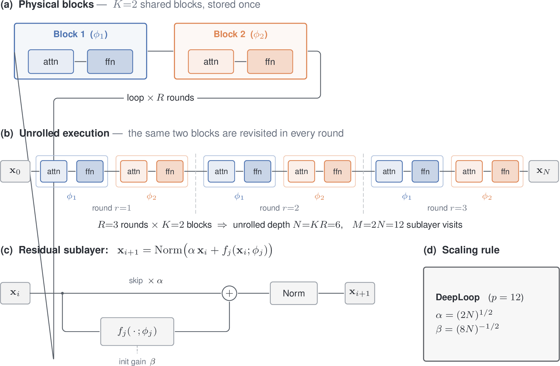
Depth is one of the most reliable ways to improve Transformer expressivity, but in standard architectures, depth and parameter count grow together: adding a layer also adds a new set of attention and feed-forward weights [1]–[3]. Looped Transformers decouple these axes by applying a stack of \(K\) physical blocks for \(R\) rounds, yielding unrolled depth \(N=KR\) while storing only \(K\) blocks (Figure 1). This mechanism connects classical depth-wise sharing in Universal Transformers, ALBERT, and Subformer [4]–[6] with recent recurrent-depth and test-time-compute models that spend additional sequential computation without a proportional increase in parameters [7]–[11]. For the looped depth to become a practical scaling axis, however, its residual parameterization must remain stable as the same physical blocks are revisited many times.
The difficulty is that standard residual-scaling analyses are written for untied depth. Residual parameterization is decisive for deep Transformer optimization [12]–[17]. DeepNorm, in particular, makes very deep Post-LN Transformers trainable by choosing a skip scale \(\alpha\) and a residual-branch initialization gain \(\beta\) so that the first-order effect of parameter updates remains bounded across \(M=2N\) residual sublayer visits [17]. This calculation assumes that each unrolled residual sublayer owns a distinct parameter tensor and therefore contributes one independent update term.
Weight sharing violates precisely this assumption. When a physical sublayer is visited \(R\) times, its optimizer update aggregates the visit-wise gradients from all rounds. The updated tensor is then reused by all of those visits in the next linearized forward computation. Tied depth therefore creates two coupled aggregation paths: the update is written by many visits and then read by many visits. The size of this effect depends on visit alignment. If visit-wise gradients and sensitivities are nearly orthogonal across rounds, a looped model behaves like untied depth up to constants. If they are coherent, the shared update can acquire an additional factor of \(R\).
This paper makes the tied-depth effect explicit. We introduce a visit-alignment coefficient \(\kappa_R\) and show that the first-order stability condition for a looped Transformer becomes \[M\kappa_R\left(\frac{\beta}{\alpha}\right)^2 = O(1),\] rather than the untied DeepNorm condition \(M(\beta/\alpha)^2=O(1)\). For the scaling family \(\alpha=(cN)^p\) and \(\beta=(dN)^{-p}\), the usual DeepNorm threshold \(p=1/4\) is recovered when visits decorrelate. In the conservative aligned regime, where \(\kappa_R=\Theta(R)\) and \(K\) is fixed while \(R\) grows, the threshold becomes \(p=1/2\).
The resulting method is DeepLoop: keep the DeepNorm Post-LN architecture, but use the loop-aware scaling rule \[\alpha=(2N)^{1/2}, \qquad \beta=(8N)^{-1/2}.\] DeepLoop introduces no gates, learned residual coefficients, auxiliary losses, or architecture-specific tuning constants. It is a deterministic residual parameterization for the regime where effective depth is increased by revisiting shared blocks.
We evaluate DeepLoop in controlled GPT-style looped language modeling ablations at GPT-2 small and GPT-2 medium scales. DeepLoop is essentially neutral at \(R=1\), where no physical block is revisited, and consistently improves final validation loss at larger loop counts. The advantage transfers to an eight-task language-model evaluation suite: downstream averages are close at \(R=1\) and move in favor of DeepLoop as recurrent depth grows. These results support the central prediction of the analysis: residual scaling should depend on how depth is realized, not only on the nominal number of unrolled layers.
Our contributions are:
We identify the tied-depth aggregation mechanism that is absent from untied residual-scaling analyses: a shared update is accumulated across repeated visits and then read through those same visits;
We derive a loop-aware first-order perturbation bound with an explicit visit-alignment coefficient \(\kappa_R\), recovering DeepNorm in the decorrelated regime and yielding a \(p=1/2\) exponent threshold in the aligned fixed-physical-depth regime;
We propose DeepLoop, the scaling rule \(\alpha=(2N)^{1/2}\) and \(\beta=(8N)^{-1/2}\), as a one-line conservative parameterization for Post-LN looped Transformers;
We provide controlled pre-training and downstream ablations at GPT-2 small and GPT-2 medium scale, showing that the correction becomes useful precisely when the loop count is greater than one.
2 Background↩︎
2.1 Looped Transformers and effective depth↩︎
A standard depth-\(N\) Transformer applies \(N\) distinct blocks once. A looped Transformer instead chooses \(K\) physical blocks and applies them for \(R\) rounds, \[\mathbf{x}_{r,k+1} = B_k(\mathbf{x}_{r,k};\phi_k), \qquad k=1,\ldots,K,\quad r=1,\ldots,R, \qquad \mathbf{x}_{r+1,1}=\mathbf{x}_{r,K+1},\] so the effective depth is \(N=KR\) while the block parameters \(\phi_1,\ldots,\phi_K\) are stored only once. The Universal Transformer [4] corresponds to the fully recurrent extreme in which the same transition is reused across depth; ALBERT [5] similarly ties Transformer parameters across layers. The regime studied here keeps \(K\) fixed or small and increases \(R\), thereby increasing test-time compute and unrolled depth without increasing the number of physical blocks.
2.2 Residual normalization↩︎
Let \(g_\ell\) denote one residual sublayer, either attention or an MLP. The two common normalization placements are \[\begin{align} \text{Pre-LN:}\quad \mathbf{x}_{\ell+1} = \mathbf{x}_\ell + g_\ell(\mathrm{Norm}(\mathbf{x}_\ell)), \qquad \text{Post-LN:}\quad \mathbf{x}_{\ell+1} = \mathrm{Norm}\left(\mathbf{x}_\ell + g_\ell(\mathbf{x}_\ell)\right). \end{align}\] Pre-LN improves optimization stability in deep Transformers, while Post-LN can preserve a more expressive residual stream [12], [13]. DeepNorm [17] modifies the Post-LN residual path by scaling the skip connection before normalization: \[\begin{align} \mathbf{x}_{\ell+1} = \mathrm{Norm}\left(\alpha\,\mathbf{x}_\ell + g_\ell(\mathbf{x}_\ell;\theta_\ell)\right). \end{align}\] For an encoder-only or decoder-only Transformer with \(N\) blocks and \(M=2N\) residual sublayer applications, DeepNorm sets \[\alpha=(2N)^{1/4}, \qquad \beta=(8N)^{-1/4}, \label{eq:deepnorm-scales-background}\tag{1}\] Here \(\beta\) is an initialization gain, not an additional runtime multiplier on the residual stream. If \(\mathcal{S}^{\mathrm{DN}}_\ell\) denotes the residual-branch matrices scaled by DeepNet in sublayer \(\ell\), such as the value and output projections in attention and the feed-forward matrices, then DeepNorm initializes \[W_{\ell,q}^{(0)} = \beta_{\mathrm{DN}}\, \widetilde{W}_{\ell,q}^{(0)}, \qquad q\in\mathcal{S}^{\mathrm{DN}}_\ell, \qquad \beta_{\mathrm{DN}}=(8N)^{-1/4}, \label{eq:deepnorm-beta-usage}\tag{2}\] with the usual unscaled initializer used for \(\widetilde{W}_{\ell,q}^{(0)}\). The quantity that enters the perturbation argument is therefore \[\frac{\beta_{\mathrm{DN}}}{\alpha_{\mathrm{DN}}} = \frac{(8N)^{-1/4}}{(2N)^{1/4}} = \frac{1}{2\sqrt{N}}. \label{eq:deepnorm-beta-over-alpha-background}\tag{3}\] The useful way to summarize the DeepNorm calculation is not a bound on \(\alpha^2\beta\), but the first-order update condition \[M\left(\frac{\beta}{\alpha}\right)^2 = \Theta(1). \label{eq:deepnorm-condition-background}\tag{4}\] Indeed, substituting Eq. (3 ) gives \(2N(\beta/\alpha)^2=1/2\).
2.3 Why weight sharing changes the depth scaling↩︎
In a non-shared depth-\(N\) Transformer, each sublayer parameter receives one gradient contribution per input. In a looped Transformer, the same physical parameter is visited once per round, so its gradient is a sum over \(R\) visits. If the visit-wise contributions decorrelate, the loop behaves like untied depth up to constants. If the visits are aligned, the tied update can be \(R\) times larger, and that same update is then read by all \(R\) visits in the unrolled computation. DeepLoop is the corresponding conservative correction to Eq. (4 ): it chooses a smaller update-to-residual ratio \(\beta/\alpha\) so that the first-order effect of the tied parameter update remains bounded after all \(R\) visits are unrolled.
3 DeepLoop Transformer↩︎
A looped Transformer reuses the same \(K\) physical blocks for \(R\) rounds. Its unrolled depth is \(N=KR\), and the number of residual-sublayer visits is \(M=2N\). DeepLoop keeps the DeepNorm architecture but uses the exponent \(p=1/2\) rather than \(p=1/4\) in the fixed-physical-depth, increasing-loop-count regime. The derivation separates two facts: RMSNorm exposes the residual branch through a factor \(1/\alpha\), and parameter tying changes the first-order update sum from \(M\) terms to \(M\kappa_R\) terms, where \(\kappa_R\) measures alignment across loop visits.
3.1 Setup: looped post-normalized block↩︎
Each physical block contains two residual sublayers: attention and MLP. Let \(j=(k,s)\) index a physical sublayer, with \(k\in\{1,\ldots,K\}\) and \(s\in\{\mathrm{attn},\mathrm{ffn}\}\), and let \(i=(r,j)\) denote its \(r\)-th unrolled visit. We write \(J=2K\) for the number of physical residual sublayers and \(M=JR=2KR=2N\) for the number of unrolled visits. DeepLoop uses \[\begin{align} \mathbf{x}_{i+1} = \mathrm{Norm}\left( \alpha\,\mathbf{x}_i + f_j(\mathbf{x}_i;\phi_j) \right), \qquad i=1,\ldots,M, \end{align}\] where the same physical parameter \(\phi_j\) is reused for all \(r=1,\ldots,R\). In our implementation, \(\mathrm{Norm}\) is RMSNorm. The gain \(\beta\) is a per-matrix initialization gain applied to the residual-branch matrices specified by DeepNorm. It should not be read as the standard deviation of the whole sublayer output, since a branch may contain multiple scaled matrices. Concretely, for each physical sublayer \(j\), let \(\mathcal{S}_j\) be the set of matrices that receive the DeepNorm gain. DeepLoop initializes \[W_{j,q}^{(0)} = \beta_{\mathrm{DL}}\, \widetilde{W}_{j,q}^{(0)}, \qquad q\in\mathcal{S}_j, \qquad \beta_{\mathrm{DL}}=(8N)^{-1/2}. \label{eq:deeploop-beta-usage}\tag{5}\] The forward recurrence then uses these initialized parameters through \(f_j(\mathbf{x}_i;\phi_j)\) at every visit; \(\beta\) is not re-applied as a separate multiplicative factor on each visit. With \(\alpha_{\mathrm{DL}}=(2N)^{1/2}\), the DeepLoop update-to-residual ratio is \[\frac{\beta_{\mathrm{DL}}}{\alpha_{\mathrm{DL}}} = \frac{(8N)^{-1/2}}{(2N)^{1/2}} = \frac{1}{4N}. \label{eq:deeploop-beta-over-alpha-setup}\tag{6}\]
Assumption 1 (DeepNorm-scale local sensitivity). For each unrolled visit \(i=(r,j)\), the norm of the linearized output map from a residual-branch parameter perturbation at that visit and the norm of the corresponding visit-wise effective update are both \(O(\beta/\alpha)\).
Assumption 1 is the local scaling condition used in the DeepNet perturbation argument. Constants depending on width, normalization gain, attention heads, learning rate, or optimizer preconditioning are absorbed into the \(O(\cdot)\) notation. The looped analysis below changes only how the visit-wise terms are aggregated when parameters are tied.
3.2 Forward stability↩︎
RMSNorm restores unit RMS at every sublayer, so the forward signal scale is not the binding constraint; the relevant constraint is the first-order sensitivity of the final output to a residual-branch parameter update. A direct expansion of \(\mathrm{RMSNorm}(\alpha\mathbf{x}+\mathbf{z})\) around \(\mathrm{RMS}(\mathbf{z})/\alpha\to 0\) shows that the residual branch enters the normalized direction through a factor of \(1/\alpha\), which is why the relevant DeepNorm ratio is \(\beta/\alpha\) rather than \(\beta\) alone. The formal statement and proof are Lemma 1 in Appendix 8.
3.3 Depth-untied DeepNorm bound↩︎
The DeepNet perturbation argument bounds the first-order output change \(\Delta F=F(\mathbf{x};\theta+\delta\theta)-F(\mathbf{x};\theta)\) by summing visit-wise sensitivities. Here depth-untied means that residual-sublayer parameters are not shared across unrolled depth. This is orthogonal to the standard tying of input and output token embeddings: tied embeddings, when used, are outside the \(M=2N\) residual-sublayer count and are not among the residual-branch matrices scaled by \(\beta\). Under Assumption 1, each visit contributes an output sensitivity \(O(\beta/\alpha)\) and an effective update \(O(\beta/\alpha)\), so summing \(M=2N\) depth-untied residual-sublayer visits gives \[\|\Delta F\| \le C'\,M\left(\frac{\beta}{\alpha}\right)^2, \label{eq:update-bound}\tag{7}\] and a sufficient first-order stability condition is \[M\left(\frac{\beta}{\alpha}\right)^2 = O(1). \label{eq:deepnet-condition}\tag{8}\] The DeepNorm choice \(\alpha=(2N)^{1/4}\) and \(\beta=(8N)^{-1/4}\) satisfies \(M(\beta/\alpha)^2 = 1/2\). The formal proposition statement and proof are Proposition [prop:untied] in Appendix 8.
3.4 Loop correction: aligned visits require \(p=1/2\)↩︎
Depth-wise residual-sublayer weight sharing changes Eq. (7 ). For a physical sublayer \(j\), let \(G_{r,j}\) be the visit-wise effective update that would be applied if visit \((r,j)\) had its own depth-untied residual-branch parameter, and let \(U_{r,j}\) be the corresponding linearized output-sensitivity operator. With tied residual-sublayer parameters, the update to \(\phi_j\) is proportional to \(\sum_{r=1}^{R}G_{r,j}\), and the output perturbation reads this same update through all visits. The first-order tied perturbation therefore has the schematic double-sum form where tensor contractions and optimizer-dependent constants are absorbed into \(U_{r,j}\) and \(G_{r,j}\).
Define the visit-alignment coefficient \[\kappa_R := \max_{j\in\{1,\ldots,J\}} \frac{ \left\|\sum_{r=1}^{R} U_{r,j}\right\| \left\|\sum_{r=1}^{R} G_{r,j}\right\| }{ R C_U C_G(\beta/\alpha)^2 }, \label{eq:kappa-def}\tag{10}\] where \(\|U_{r,j}\|\le C_U\beta/\alpha\) and \(\|G_{r,j}\|\le C_G\beta/\alpha\). The triangle inequality gives \(0\le\kappa_R\le R\). Independent or nearly orthogonal visits give \(\kappa_R=O(1)\), while fully aligned visits give \(\kappa_R=\Theta(R)\).
Substituting the definition of \(\kappa_R\) from Eq. (10 ) into Eq. (9 ) and applying submultiplicativity gives the looped version of the DeepNorm bound, \[\|\Delta F\| \le C''\,M\kappa_R\left(\frac{\beta}{\alpha}\right)^2, \label{eq:loop-update-bound}\tag{11}\] so a sufficient tied-depth stability condition is \[M\kappa_R\left(\frac{\beta}{\alpha}\right)^2 = O(1). \label{eq:loop-condition}\tag{12}\] In the worst-case aligned regime \(\kappa_R=\Theta(R)\), this reduces to \(MR(\beta/\alpha)^2=O(1)\). The formal proposition and the aligned-case corollary are Proposition [prop:tied-perturbation] and Corollary 1 in Appendix 8.
Now consider the family \(\alpha=(cN)^p\), \(\beta=(dN)^{-p}\) with constants \(c,d>0\). Its update-to-residual ratio is \[\frac{\beta}{\alpha} = (cd)^{-p}N^{-2p}. \label{eq:beta-over-alpha}\tag{13}\]
Assume \(K\) is fixed, \(N=KR\), \(M=2N\), and \(\kappa_R=\Theta(R^\gamma)\) for some \(\gamma\in[0,1]\). For the scaling family \(\alpha=(cN)^p\), \(\beta=(dN)^{-p}\), the tied-depth condition \[M\kappa_R(\beta/\alpha)^2=O(1)\] holds uniformly as \(R\to\infty\) if and only if \[p\ge \frac{1+\gamma}{4}.\]
Proposition [prop:exponent-threshold] shows where the new exponent comes from. When visits decorrelate, \(\gamma=0\), and the DeepNorm threshold \(p=1/4\) is recovered. In the conservative aligned case, \(\gamma=1\), so the threshold is \(p=1/2\). Equivalently, \[M R\left(\frac{\beta}{\alpha}\right)^2 = 2NR\,(cd)^{-2p}N^{-4p}. \label{eq:p-family-loop}\tag{14}\] At fixed \(K\), \(R=N/K\), so Eq. (14 ) is bounded only when \(p\ge 1/2\). DeepNorm’s \(p=1/4\) leaves a residual growth of \(\Theta(R)\) in the aligned shared-loop bound. The DeepLoop choice is \[\begin{align} \alpha=(2N)^{1/2}, \qquad \beta=(8N)^{-1/2}. \end{align}\] We keep the DeepNorm constants \((c,d)=(2,8)\) for a two-sublayer decoder block and change only the exponent. Equivalently, DeepLoop uses the same per-matrix definition as Eq. (5 ) with \(\beta=\beta_{\mathrm{DL}}\). With this choice, \[\frac{\beta}{\alpha} = \frac{1}{4N}, \qquad MR\left(\frac{\beta}{\alpha}\right)^2 = 2NR\cdot \frac{1}{16N^2} = \frac{1}{8K},\] so the worst-case aligned tied-depth bound remains \(O(1)\) at fixed physical depth \(K\). Proofs of Proposition [prop:tied-perturbation] and Proposition [prop:exponent-threshold] are in Appendix 8. Appendix 10 sweeps \(p\) over a single grid at \(R{=}3\) and finds an empirical training-stability boundary that lines up with this \(p{=}1/2\) prediction.
3.5 Summary and comparison to DeepNorm↩︎
| DeepNorm | DeepLoop | |
|---|---|---|
| Residual scale \(\alpha\) | \((2N)^{1/4}\) | \((2N)^{1/2}\) |
| Init gain \(\beta\) | \((8N)^{-1/4}\) | \((8N)^{-1/2}\) |
| Per-matrix use of \(\beta\) | \(W^{(0)}\leftarrow\beta\,\widetilde{W}^{(0)}\) | \(W^{(0)}\leftarrow\beta\,\widetilde{W}^{(0)}\) |
| Update-to-residual \(\beta/\alpha\) | \(1/(2\sqrt{N})\) | \(1/(4N)\) |
| Untied bound \(M(\beta/\alpha)^2\) | \(\Theta(1)\) | \(\Theta(N^{-1})\) |
| Aligned tied-loop bound \(MR(\beta/\alpha)^2\) at fixed \(K\) | \(\Theta(R)\) | \(\Theta(1/K)\) |
DeepLoop is therefore a one-line conservative correction for tied depth: increase the exponent from \(p=1/4\) to \(p=1/2\). It introduces no gates, learnable residual scalars, or additional tuning constants. The correction is not a claim that every looped model empirically attains worst-case alignment. Rather, it is the minimal exponent for uniform boundedness under aligned visit-wise contributions at fixed physical depth.
4 Application to Hierarchical Recurrent Reasoners↩︎
The DeepLoop derivation in Section 3 treats a single looped block visited for \(R\) rounds. Recent recurrent-reasoning architectures combine looping with two further structural choices: a hierarchy of recurrent modules executed at different rates, and training-time gradient truncation across the outer recurrence [10], [18]. The Hierarchical Reasoning Model [18] instantiates both: a high-level module \(\mathcal{H}\) and a low-level module \(\mathcal{L}\) are unrolled jointly, and gradients are computed through only the last outer cycle. This section shows that the framework of Section 3 extends to this regime by replacing the unrolled visit count \(M\) with a gradient-visible visit count \(M_{\mathrm{g}}\) and tracking per-module visit counts separately. We do not introduce new optimization machinery or a new variant of DeepLoop; we describe how the existing analysis specializes when training-time depth and forward depth differ.
4.1 Setup: two-module hierarchical loops↩︎
Let \(\mathcal{H}\) contain \(K_H\) physical blocks (each with two residual sublayers, attention and MLP) and let \(\mathcal{L}\) contain \(K_L\) physical blocks of the same shape. The hierarchical recurrence runs \(C\) outer cycles; within each outer cycle, \(\mathcal{L}\) iterates \(C_L\) times before a single update of \(\mathcal{H}\): \[\text{cycle } c:\quad \mathbf{z}_L \leftarrow \mathcal{L}^{(C_L)}(\mathbf{z}_L,\mathbf{z}_H),\qquad \mathbf{z}_H \leftarrow \mathcal{H}(\mathbf{z}_H,\mathbf{z}_L), \quad c=1,\ldots,C.\] Counting attention and MLP residual sublayers, the total unrolled visit count is \[M = 2\,C\,(K_H + C_L K_L), \label{eq:hrm-forward-M}\tag{15}\] which generalizes the single-module count \(M=2KR\) used in Section 3. The set of distinct physical residual sublayers has size \(J = J_H + J_L\) with \(J_H = 2K_H\) and \(J_L = 2K_L\). Each visit \(i=(c,\ell,j)\) has an outer-cycle index \(c\), an inner \(\mathcal{L}\)-iterate index \(\ell\) (only meaningful for \(j\in\mathcal{L}\)), and a physical-sublayer index \(j\).
4.2 Loop-aware bound under one-step gradient approximation↩︎
Hierarchical recurrent reasoners are typically trained with a one-step gradient approximation: the forward pass uses all \(C\) outer cycles, but the backward pass is computed against the last cycle only, with \(\mathbf{z}_H\) and \(\mathbf{z}_L\) from earlier cycles detached from the autograd graph. This truncation does not alter the numerical forward values, so Lemma 1 applies unchanged locally. The perturbation bound below is for the truncated training graph: the states entering the last outer cycle are treated as fixed inputs, and both the sensitivity terms and the update terms from earlier cycles are absent. A perturbation bound for the full untruncated forward map after an optimizer step would require an additional forward-visible read factor.
Define the gradient-visible visit count \[M_{\mathrm{g}} := 2\,(K_H + C_L K_L), \label{eq:hrm-Mg}\tag{16}\] so \(M = C\,M_{\mathrm{g}}\). The per-physical-sublayer round counts on the gradient-visible cycle are \[R_{\mathrm{g}}^{(\mathcal{H})} = 1, \qquad R_{\mathrm{g}}^{(\mathcal{L})} = C_L. \label{eq:hrm-per-module-R}\tag{17}\] Repeating the argument leading to Eq. (11 ) but restricting the visit-index sums to the gradient-visible cycle gives the two-module loop-aware bound \[\|\Delta F\| \le C''\! \left[ J_H\,R_{\mathrm{g}}^{(\mathcal{H})}\,\kappa_{\mathrm{g}}^{(\mathcal{H})} + J_L\,R_{\mathrm{g}}^{(\mathcal{L})}\,\kappa_{\mathrm{g}}^{(\mathcal{L})} \right] \left(\frac{\beta}{\alpha}\right)^2, \label{eq:hrm-per-module-bound}\tag{18}\] where \(\kappa_{\mathrm{g}}^{(\mathcal{H})},\kappa_{\mathrm{g}}^{(\mathcal{L})}\) are the visit-alignment coefficients of Eq. (10 ) restricted to each module’s gradient-visible visits. Two structural facts simplify Eq. (18 ). First, \(\kappa_{\mathrm{g}}^{(\mathcal{H})}\le 1\) trivially: with \(R_{\mathrm{g}}^{(\mathcal{H})}=1\), each physical \(\mathcal{H}\)-sublayer contributes a single-term inner sum, and the alignment coefficient collapses to a constant. The truncation thus places \(\mathcal{H}\) in the untied-DeepNorm regime even though \(\mathcal{H}\) is forward-visited \(C\) times. Second, \(\kappa_{\mathrm{g}}^{(\mathcal{L})}\in[0,C_L]\) by the triangle inequality applied to the inner \(\mathcal{L}\)-iterate sum. Substituting these facts, upper-bounding \(\kappa_{\mathrm{g}}^{(\mathcal{H})}\) by one, and applying the per-module counts in Eq. (17 ) yields the sufficient stability condition \[M_{\mathrm{g}}\,\bar\kappa_{\mathrm{g}}\, \left(\frac{\beta}{\alpha}\right)^2 = O(1), \qquad \bar\kappa_{\mathrm{g}} := \frac{J_H + J_L\,C_L\,\kappa_{\mathrm{g}}^{(\mathcal{L})}}{M_{\mathrm{g}}}, \label{eq:hrm-cond}\tag{19}\] which has the same structural form as Eq. (12 ) with \(M\) replaced by \(M_{\mathrm{g}}\) and \(\kappa_R\) replaced by the gradient-visible aggregate \(\bar\kappa_{\mathrm{g}}\in[\,J_H/M_{\mathrm{g}},\,1+J_L C_L(C_L-1)/M_{\mathrm{g}}\,]\).
The decomposition (18 ) also licenses a per-module scaling family. Each summand depends only on the \((\alpha,\beta)\) used at the corresponding module, so a hierarchical reasoner may be parameterized with \((\alpha_{\mathcal{H}},\beta_{\mathcal{H}})\) and \((\alpha_{\mathcal{L}},\beta_{\mathcal{L}})\) chosen independently. The admissible exponent at each module is determined by the corresponding summand of Eq. (18 ), not by the global visit count.
4.3 Predicted exponent regime↩︎
Let \(N_{\mathrm{g}}:=M_{\mathrm{g}}/2\) denote the gradient-visible block-equivalent depth. Combining Eq. (19 ) with the same two-sublayer scaling family used above, \(\alpha=(c N_{\mathrm{g}})^p\), \(\beta=(d N_{\mathrm{g}})^{-p}\), gives, up to constant factors, \[M_{\mathrm{g}}\,\bar\kappa_{\mathrm{g}}\, (cd)^{-2p}\,N_{\mathrm{g}}^{-4p} = \Theta\!\left((cd)^{-2p}\,\bar\kappa_{\mathrm{g}}\,M_{\mathrm{g}}^{1-4p}\right), \label{eq:hrm-pthreshold}\tag{20}\] and the asymptotic threshold for boundedness depends on how \(\bar\kappa_{\mathrm{g}}\) and \(M_{\mathrm{g}}\) co-scale. We record the two limit cases that mirror Proposition [prop:exponent-threshold].
4.3.0.1 Decorrelated inner cycles (\(\kappa_{\mathrm{g}}^{(\mathcal{L})}=O(1)\)).
Then \(\bar\kappa_{\mathrm{g}}=O(1)\) and Eq. (20 ) is bounded as \(M_{\mathrm{g}}\to\infty\) if and only if \(p \ge 1/4.\) Both modules sit in the untied-DeepNorm regime: the \(\mathcal{H}\) module by truncation, and the \(\mathcal{L}\) module by the inner-cycle decorrelation.
4.3.0.2 Aligned inner cycles (\(\kappa_{\mathrm{g}}^{(\mathcal{L})}=\Theta(C_L)\)).
Then the \(\mathcal{L}\) contribution to \(\bar\kappa_{\mathrm{g}}\) is \(\Theta(C_L^2\,J_L/M_{\mathrm{g}})\). Two sub-cases follow from how \(M_{\mathrm{g}}\) is grown. (i) If \(C_L\) is fixed and \(K_H,K_L\to\infty\), then \(\bar\kappa_{\mathrm{g}}=\Theta(1)\) and the threshold is again \(p\ge 1/4\). (ii) If \(K_H,K_L\) are fixed and \(C_L\to\infty\), then \(M_{\mathrm{g}}=\Theta(C_L)\) and \(\bar\kappa_{\mathrm{g}}=\Theta(C_L)\), so Eq. (20 ) is bounded if and only if \(p \ge 1/2,\) which recovers the fixed-physical-depth tied-loop threshold of Proposition [prop:exponent-threshold] along the inner-cycle axis.
For a hierarchical recurrent reasoner as actually built, these two limits are not equally likely possibilities but a binding constraint and a slack one. The once-per-step \(\mathcal{H}\) module is truncated by the one-step gradient, contributes a single update term, and therefore requires only \(p\ge 1/4\). The \(\mathcal{L}\) module is the one that realizes the model’s effective depth: it revisits its shared blocks at fixed physical depth, the \(C_L\) axis of sub-case (ii), and weight tying is adopted precisely so that those revisits implement the same operation, which aligns their visit-wise gradients and sensitivities (\(\kappa_{\mathrm{g}}^{(\mathcal{L})}=\Theta(C_L)\)). The \(\mathcal{L}\) module therefore requires \(p\ge 1/2\). A single shared residual exponent must satisfy the more demanding module, so the framework predicts \[p = 1/2 \label{eq:hrm-p-prediction}\tag{21}\] for a hierarchical recurrent reasoner, the same loop-aware exponent as the single-module backbone of Section 3. This is a statement about the architecture as trained, not a conservative envelope: the recurrent depth that makes the model work is grown along the aligned inner-cycle axis, exactly the regime whose threshold is \(1/2\), and \(p=1/2\) simultaneously satisfies the once-per-step module (for which \(1/2\ge 1/4\)). Section 5 confirms the prediction empirically on ARC-AGI.
4.3.0.3 Forward signal at the loop entry.
A practical detail of hierarchical reasoners is the addition of a learned task or puzzle embedding \(\mathbf{e}_{\mathrm{task}}\) to the token embedding \(\mathbf{e}_{\mathrm{tok}}\) before the loop. The choice of whether to apply RMSNorm to \(\mathbf{e}_{\mathrm{tok}}+\mathbf{e}_{\mathrm{task}}\) at the loop entry affects only the forward signal scale \(\mathrm{RMS}(\mathbf{x}_0)\) in Lemma 1; it does not enter Eq. (18 ) or the threshold derivation (20 ). Input-side normalization and the residual scaling rule are therefore separable design choices within this framework, even though both can independently influence the relative magnitude of task-conditioning information across repeated visits.
4.4 Summary↩︎
The DeepLoop perturbation argument extends to hierarchical recurrent reasoners by two substitutions. When training uses a one-step gradient approximation, the visit count entering the bound is the gradient-visible \(M_{\mathrm{g}}\) from Eq. (16 ) rather than the forward \(M\) from Eq. (15 ). When the architecture splits the recurrence across modules with different per-step visit counts, the bound decomposes into per-module summands and admits asymmetric per-module \((\alpha,\beta)\) assignments. Because a hierarchical recurrent reasoner grows its effective depth by aligned revisits of the shared inner module at fixed physical depth, the binding threshold from Eq. (20 ) is \(p=1/2\), the same loop-aware exponent as the single-module backbone. Section 5 confirms this on ARC-AGI: the DeepLoop exponent \(p=1/2\) improves voted accuracy over the vanilla HRM baseline across the full evaluation ladder.
5 Experiments↩︎
5.1 Validation loss↩︎
We compare DeepLoop against a baseline that already incorporates the same looped residual-block sharing, tied input-output embeddings, and an input-embedding RMSNorm. The baseline (base) uses this same looped backbone and embedding tying,
but keeps the residual and initialization scales at \(\alpha=1\) and \(\beta=1\). The DeepLoop variant additionally enables the scaling rule on every block. Both configurations share an
identical backbone, optimizer, data pipeline, and random seed; the only knob that moves between rows of Table 1 is the loop count \(R \in \{1,3,5,7\}\), and the only knob that moves
between methods is the activation of DeepLoop.
The GPT-2 small runs use a GPT-MHA-RoPE model trained on FineWeb-Edu for 50B tokens (100K optimizer steps, context length 1024, global batch size 480) on 4\(\times\)H200 141GB GPUs. The GPT-2 medium runs use the same backbone with hidden size enlarged from \(768\) to \(1024\) and the number of layers doubled from \(12\) to \(24\), trained on the same data and schedule on 8\(\times\)H200 141GB GPUs. We report the validation cross-entropy at the final checkpoint for both scales in Table 1.
| Method | \(R=1\) | \(R=3\) | \(R=5\) | \(R=7\) |
|---|---|---|---|---|
| GPT-2 small backbone | ||||
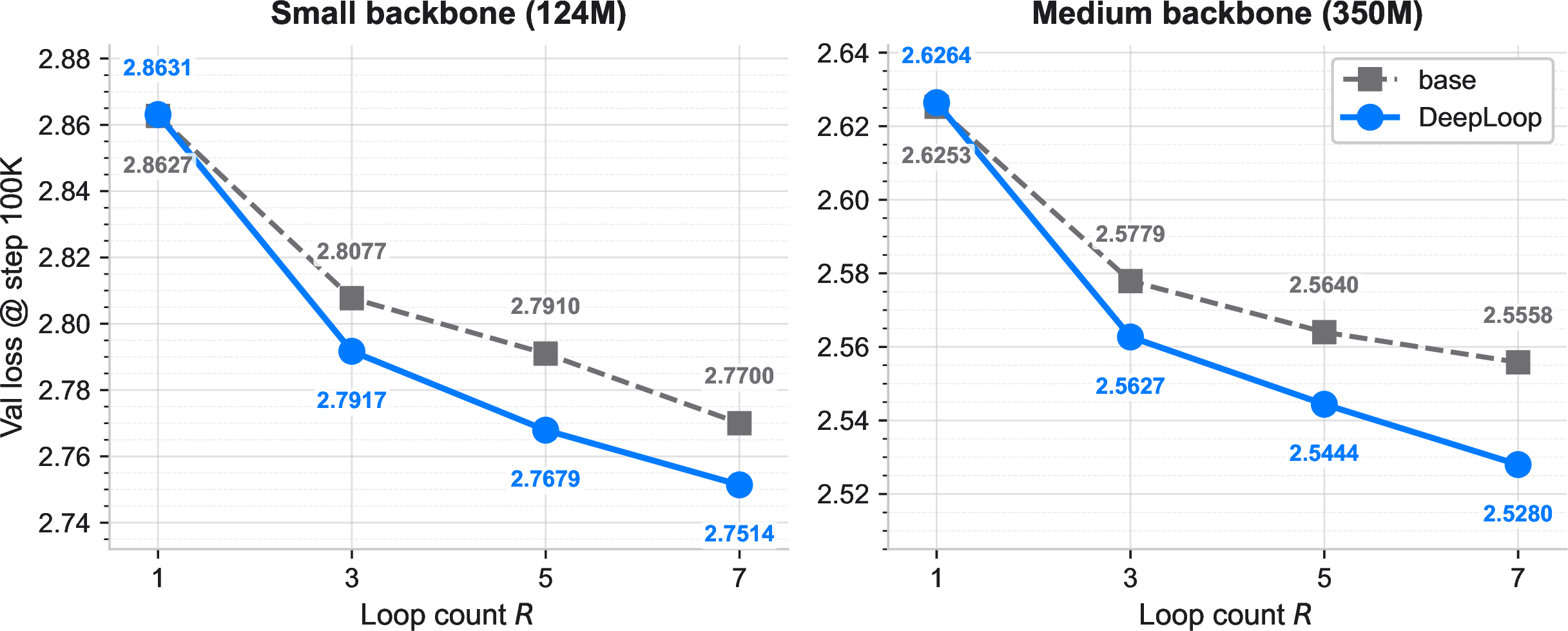
| baseline (tying + input-embed RMSNorm) | 2.8627 | 2.8077 | 2.7910 | 2.7700 |
| DeepLoop | 2.8631 | 2.7917 | 2.7679 | 2.7514 |
| \(\Delta\) (DeepLoop \(-\) base) | \(+0.0004\) | \(-0.0160\) | \(-0.0231\) | \(-0.0186\) |
| GPT-2 medium backbone | ||||
| baseline (tying + input-embed RMSNorm) | 2.6253 | 2.5779 | 2.5640 | 2.5558 |
| DeepLoop | 2.6264 | 2.5627 | 2.5444 | 2.5280 |
| \(\Delta\) (DeepLoop \(-\) base) | \(+0.0011\) | \(-0.0153\) | \(-0.0196\) | \(-0.0278\) |
Figure 2 visualizes the same numbers as Table 1. At both scales the two curves coincide within noise at \(R{=}1\) (\(+0.0004\) and \(+0.0011\) nats) and separate as the loop count grows: at the small scale DeepLoop pulls ahead by \(-0.016\) nats at \(R{=}3\), the gap peaks at \(-0.023\) nats at \(R{=}5\), and remains open at \(-0.019\) nats at \(R{=}7\); at the medium scale the gap widens monotonically through \(R{=}7\), reaching \(-0.028\) nats. Both methods continue to improve monotonically with \(R\) at both scales, and DeepLoop strictly beats the baseline at every \(R\geq3\). Multi-seed runs would be needed to quantify run-to-run variance.
5.2 Downstream evaluation on the lm-evaluation-harness suite↩︎
To test whether the validation-loss advantage transfers to downstream task accuracy, we evaluate the eight medium-scale checkpoints from §5.1 on the eight-task zero- and one-shot suite used by [19] in the Deep Delta Learning paper: arc_challenge, arc_easy, hellaswag, openbookqa,
piqa, sciq, social_iqa, and winogrande. Evaluation uses the lm-evaluation-harness [20] with its default acc metric (not acc_norm), the GPT-2 tokenizer, a context length of 1024 (matching training), and bf16 inference. The reported Avg column is the unweighted arithmetic
mean of the eight per-task accuracies, following the protocol of [19].
Table 2 reports the per-task accuracy and Avg for every (method, \(R\), shot) cell at the medium scale. Figure 3 breaks the 1-shot column out task-by-task. The corresponding GPT-2 small downstream results, which exhibit the same qualitative pattern, are deferred to Appendix 9.
| Method / \(R\) | ARC-C | ARC-E | HellaSwag | OBQA | PIQA | SciQ | SIQA | WG | Avg |
|---|---|---|---|---|---|---|---|---|---|
| 0-shot | |||||||||
| baseline \(R{=}1\) | 29.44 | 65.24 | 38.12 | 23.60 | 69.80 | 85.80 | 40.23 | 54.70 | 50.86 |
| baseline \(R{=}3\) | 32.59 | 66.75 | 39.76 | 27.60 | 70.13 | 87.30 | 39.87 | 55.96 | 52.50 |
| baseline \(R{=}5\) | 33.53 | 68.31 | 41.01 | 25.80 | 69.70 | 88.20 | 38.95 | 55.41 | 52.61 |
| baseline \(R{=}7\) | 32.34 | 69.40 | 40.61 | 24.40 | 70.67 | 89.20 | 39.66 | 57.30 | 52.95 |
| DeepLoop \(R{=}1\) | 29.86 | 65.07 | 38.21 | 23.60 | 68.82 | 86.10 | 39.92 | 55.25 | 50.85 |
| DeepLoop \(R{=}3\) | 32.59 | 68.43 | 40.85 | 26.80 | 70.29 | 88.30 | 40.02 | 56.12 | 52.93 |
| DeepLoop \(R{=}5\) | 33.53 | 68.60 | 41.78 | 28.20 | 70.46 | 90.10 | 40.58 | 56.12 | 53.67 |
| DeepLoop \(R{=}7\) | 33.11 | 69.65 | 41.83 | 25.60 | 70.57 | 90.30 | 40.94 | 59.04 | 53.88 |
| 1-shot | |||||||||
| baseline \(R{=}1\) | 30.38 | 66.92 | 37.73 | 24.20 | 70.08 | 88.30 | 40.79 | 55.09 | 51.69 |
| baseline \(R{=}3\) | 33.70 | 68.69 | 39.71 | 26.00 | 70.13 | 90.50 | 40.74 | 55.33 | 53.10 |
| baseline \(R{=}5\) | 35.75 | 70.88 | 40.82 | 27.80 | 71.60 | 91.90 | 39.71 | 56.91 | 54.42 |
| baseline \(R{=}7\) | 34.22 | 70.54 | 40.87 | 27.80 | 71.33 | 92.10 | 41.30 | 58.80 | 54.62 |
| DeepLoop \(R{=}1\) | 30.80 | 65.78 | 37.73 | 22.80 | 69.10 | 89.50 | 41.30 | 55.25 | 51.53 |
| DeepLoop \(R{=}3\) | 33.11 | 68.14 | 40.59 | 26.20 | 69.48 | 91.30 | 41.15 | 57.38 | 53.42 |
| DeepLoop \(R{=}5\) | 36.43 | 68.18 | 41.50 | 26.00 | 70.84 | 92.10 | 40.99 | 57.46 | 54.19 |
| DeepLoop \(R{=}7\) | 35.15 | 70.96 | 41.83 | 28.80 | 70.51 | 92.40 | 42.53 | 59.43 | 55.20 |
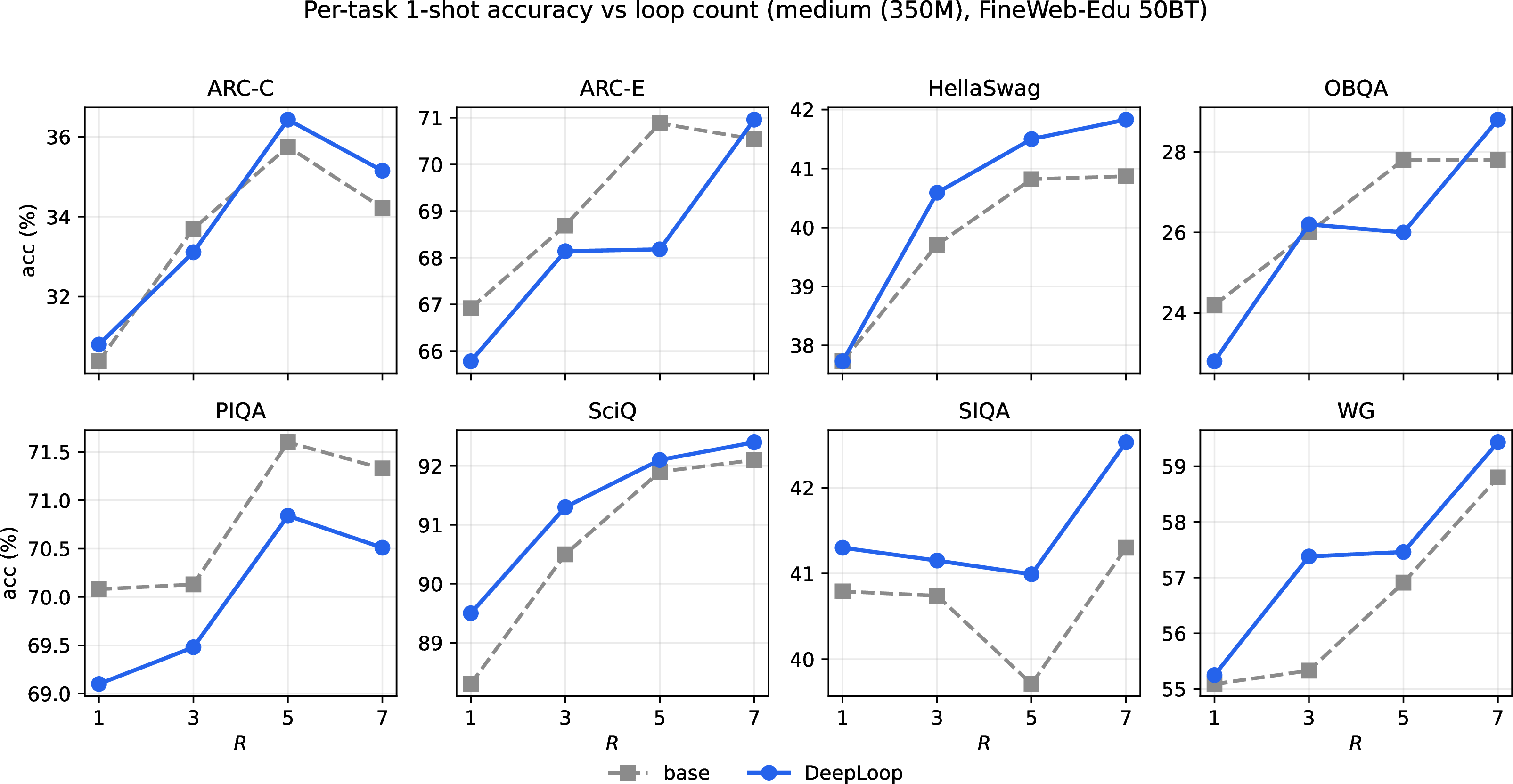
Two takeaways. First, the qualitative picture from the small-scale ablation (Appendix Table 4) carries over to the larger backbone: the two methods are tied at \(R{=}1\) (\(\Delta=-0.01\) on the 0-shot Avg, \(-0.16\) on 1-shot), DeepLoop opens the gap at \(R{=}3\) (\(+0.43\) / \(+0.32\)), and the best Avg cell in the table is DeepLoop \(R{=}7\) in both shot settings, headlined by \(55.20\,\%\) on 1-shot. On the 0-shot Avg the gap widens through \(R{=}7\) (\(+0.43\), \(+1.06\), \(+0.93\)); on the 1-shot Avg the ranking is messier at \(R{=}5\) (where the base reaches \(54.42\,\%\), \(0.23\) points above DeepLoop) but DeepLoop recovers the lead by \(+0.58\) points at \(R{=}7\). Second, at \(R{=}7\) DeepLoop beats the same-\(R\) baseline on seven of the eight individual tasks under both shot settings (only PIQA goes the other way), with WinoGrande in particular jumping by \(+1.74\) points 0-shot (\(59.04\) vs.\(57.30\)). The same caveat about single-seed run-to-run variance from §5.1 applies, we see no qualitative disagreement with the small-scale ablation, only a stronger depth signal.
5.3 Reasoning evaluation on ARC-AGI↩︎
To test the prediction of Eq. (21 ) on a hierarchical recurrent reasoner, we apply the DeepLoop scaling rule with \(p=1/2\) to the Hierarchical Reasoning Model (HRM) [18] and evaluate on ARC-AGI-1 [21]. The only change from the published HRM is the residual parameterization: every reasoning block uses \(\alpha=(2N_{\mathrm{g}})^{1/2}\) and \(\beta=(8N_{\mathrm{g}})^{-1/2}\) with \(M_{\mathrm{g}}=24\) gradient-visible residual-sublayer visits and \(N_{\mathrm{g}}=M_{\mathrm{g}}/2=12\) block-equivalent
depth (Eq. 16 ); the backbone, the adaptive-computation halting, the optimizer (AdamATan2), the data pipeline, and the 100K-epoch schedule are held fixed. Baseline and DeepLoop runs train on an identical, hash-verified
arc-aug-1000 build and are scored by the same count-first voting protocol on \(N=400\) evaluation puzzles. As a harness check, the published HRM ARC-2 checkpoint scores \(5.00\%\) (\(K{=}2\)) on this pipeline, matching the released value.
Table 3 reports voted accuracy at voting budgets \(K\in\{1,2,10,100,1000\}\). DeepLoop improves the paper-protocol two-vote accuracy from \(36.50\%\) to \(39.75\%\) (\(+3.25\) pp) and improves every column of the voting ladder. A four-seed control places the per-seed \(K{=}2\) standard deviation at \(\approx 0.5\) pp, so the \(+3.25\) pp gain is roughly a \(6\sigma\) effect rather than a seed draw. The prediction that a tied hierarchical reasoner sits at the aligned \(p=1/2\) threshold, the same exponent that is optimal for the single-module looped backbone (Table 1), is therefore borne out: a single residual-scaling rule, \(p=1/2\), is the correct setting for both the looped language model and the hierarchical recurrent reasoner.
| Method | \(K{=}1\) | \(K{=}2\) | \(K{=}10\) | \(K{=}100\) | \(K{=}1000\) |
|---|---|---|---|---|---|
| Vanilla HRM | 31.50 | 36.50 | 41.50 | 47.50 | 50.75 |
| DeepLoop (\(p{=}1/2\)) | 35.50 | 39.75 | 44.25 | 49.75 | 51.50 |
| \(\Delta\) | \(+4.00\) | \(+3.25\) | \(+2.75\) | \(+2.25\) | \(+0.75\) |
6 Related Work↩︎
6.0.0.1 Looped and universal Transformers.
Universal Transformers [4] and ALBERT [5] introduced depth-wise parameter sharing as a way to increase effective computation without increasing parameter count. Later work studied partial sharing [6], looped Transformers for in-context learning and algorithmic computation [7]–[9], and recurrent-depth language models that trade inference compute for quality [10]. DeepLoop is orthogonal to these architectures: it only changes the residual and initialization scales used when a physical block is revisited.
6.0.0.2 Adaptive computation and iterative reasoning.
Looped depth can also be viewed as a differentiable test-time-compute mechanism. Adaptive Computation Time [22], PonderNet [23], and recurrent networks for algorithmic extrapolation [24], [25] all exploit repeated application of shared computation. Recent language-modeling work similarly adds latent or recurrent computation [11], [26], [27]. Our analysis targets the stability of this repeated shared computation.
6.0.0.3 Residual scaling and parameterization.
Transformer stability has been improved through normalization placement [12], [13], initialization and residual scaling [14]–[16], [28], [29], and DeepNorm/DeepNet [17], which derives \(\alpha=(2N)^{1/4}\) and \(\beta=(8N)^{-1/4}\) for untied Post-LN Transformers. Width-and-depth parameterizations such as \(\mu\)P and Depth-\(\mu\)P prescribe complementary scalings for feature learning and hyperparameter transfer [30]–[33]. These analyses do not explicitly account for the extra correlation introduced when the same residual-branch parameters are reused across loop visits. DeepLoop is a loop-specific correction to the DeepNorm exponent.
7 Conclusion↩︎
Looped Transformers turn depth into a controllable compute resource, but repeated parameter reuse changes the residual-scaling problem. When a residual branch is revisited, its shared update is accumulated across visits and then read by those same visits in the next linearized forward pass. We captured this tied-depth effect with a visit-alignment coefficient \(\kappa_R\), recovering the DeepNorm exponent for decorrelated visits and identifying \(p=1/2\) as the conservative exponent for aligned visits at fixed physical depth.
DeepLoop implements this correction with a one-line Post-LN scaling rule, \(\alpha=(2N)^{1/2}\) and \(\beta=(8N)^{-1/2}\). Empirically, it is neutral when no physical block is revisited and improves looped GPT-style language models as recurrent depth increases, with gains in validation loss and downstream accuracy. A \(p\)-sweep at \(R{=}3\) further places the stability boundary near \(p=1/2\).
Future work should measure \(\kappa_R\) or cross-round gradient alignment directly, test whether the same boundary holds at larger scale or under alternative parameterizations, and explore whether training can encourage decorrelated visits to safely use less conservative exponents.
Acknowledgement↩︎
We thank Zixuan Wang and Eric Song for their constructful feedback and insightful discussion.
8 Proofs↩︎
Lemma 1 (RMSNorm exposes the residual branch through \(1/\alpha\)). Let \(\mathrm{RMS}(x)^2=d^{-1}\|x\|^2\), assume \(\mathrm{RMS}(x)=1\), and define \(\mathcal{R}(y)=y/\mathrm{RMS}(y)\). If \(\mathrm{RMS}(z)/\alpha\le c<1\), then \[\mathcal{R}(\alpha x+z) = x + \frac{z-\langle x,z\rangle_d x}{\alpha} + O\left(\frac{\mathrm{RMS}(z)^2}{\alpha^2}\right), \qquad \langle x,z\rangle_d := d^{-1}x^\top z . \label{eq:rmsnorm-expansion}\qquad{(1)}\]
Proof of Lemma 1. Write \(m=\langle x,z\rangle_d\) and \(\delta^2=\mathrm{RMS}(z)^2\). Since \(|m|\le\delta\) and \(\delta/\alpha\le c<1\), the quantity below is bounded away from zero: \[\mathrm{RMS}(\alpha x+z) =\alpha\left(1+2m/\alpha+\delta^2/\alpha^2\right)^{1/2}.\] A first-order Taylor expansion of the inverse square root around one gives \[\left(1+2m/\alpha+\delta^2/\alpha^2\right)^{-1/2} =1-m/\alpha+O(\delta^2/\alpha^2),\] where the remainder is uniform for \(\delta/\alpha\le c\). Multiplying by \((\alpha x+z)/\alpha\) yields \[\frac{\alpha x+z}{\mathrm{RMS}(\alpha x+z)} =x+\frac{z-mx}{\alpha}+O(\delta^2/\alpha^2),\] which is Eq. (?? ). ◻
For a depth-\(N\) post-normalized Transformer whose residual-sublayer parameters are not shared across unrolled depth, with \(M=2N\) residual-sublayer visits, Assumption 1 implies the first-order bound Eq. (7 ), and consequently \(M(\beta/\alpha)^2=O(1)\) (Eq. (8 )) is a sufficient first-order stability condition. This statement does not depend on whether the input and output token embeddings are tied.
Proof of Proposition [prop:untied]. In the depth-untied residual stack, every unrolled residual-sublayer visit has its own residual-branch parameter tensor. The first-order change is therefore a sum of \(M\) independent visit-wise perturbation terms. By Assumption 1, each term is bounded by an output sensitivity \(O(\beta/\alpha)\) times an effective update \(O(\beta/\alpha)\). Summing over \(M\) visits gives \[\|\Delta F\| \le C' M (\beta/\alpha)^2,\] for a depth-independent constant \(C'\), which implies the stated sufficient condition. ◻
Under Assumption 1, a looped Transformer with \(J=2K\) physical residual sublayers and \(R\) visits satisfies the first-order bound Eq. (11 ), so \(M\kappa_R(\beta/\alpha)^2=O(1)\) (Eq. (12 )) is a sufficient tied-depth stability condition.
Corollary 1 (Worst-case aligned loop bound). If \(\kappa_R=\Theta(R)\), then Eq. (12 ) reduces to \(MR(\beta/\alpha)^2 = O(1)\).
Proof of Proposition [prop:tied-perturbation]. Using Eq. (9 ) and submultiplicativity, \[\|\Delta F_{\mathrm{tied}}\| \le \eta\sum_{j=1}^{J} \left\|\sum_{r=1}^{R} U_{r,j}\right\| \left\|\sum_{t=1}^{R} G_{t,j}\right\| +O(\eta^2).\] By the definition of \(\kappa_R\), each physical sublayer contributes at most \(R\kappa_R C_UC_G(\beta/\alpha)^2\). Summing over \(J\) physical sublayers gives \[JR\kappa_R C_UC_G(\beta/\alpha)^2 =M\kappa_R C_UC_G(\beta/\alpha)^2.\] Absorbing \(\eta\), \(C_U\), and \(C_G\) into the constant proves Eq. (11 ). ◻
Proof of Proposition [prop:exponent-threshold]. Substituting Eq. (13 ) into the tied-depth condition gives \[M\kappa_R\left(\frac{\beta}{\alpha}\right)^2 =2N\,\Theta(R^\gamma)\,(cd)^{-2p}N^{-4p}.\] At fixed physical depth \(K\), \(R=N/K\), so the \(N\)-dependence is \(\Theta(N^{1+\gamma-4p})\). This quantity remains uniformly bounded as \(R\to\infty\) if and only if \(1+\gamma-4p\le0\), equivalently \(p\ge(1+\gamma)/4\). ◻
9 Small-scale downstream evaluation↩︎
We report the GPT-2 small version of the downstream evaluation from §5.2. The architecture is identical to the medium backbone except for hidden size \(768\) (vs.\(1024\)) and \(12\) layers (vs.\(24\)); training uses the same FineWeb-Edu 50BT data and schedule but on \(4\times\)H200 141 GB
GPUs. The same eight-task lm-evaluation-harness protocol applies. Table 4 reports per-task accuracy and Avg; Figures 4 and 5 visualize the 1-shot Avg and the per-task 1-shot accuracy, respectively.
| Method / \(R\) | ARC-C | ARC-E | HellaSwag | OBQA | PIQA | SciQ | SIQA | WG | Avg |
|---|---|---|---|---|---|---|---|---|---|
| 0-shot | |||||||||
| base \(R{=}1\) | 23.12 | 57.11 | 31.95 | 20.60 | 65.83 | 81.90 | 37.87 | 51.62 | 46.25 |
| base \(R{=}3\) | 23.89 | 60.40 | 33.70 | 20.20 | 66.76 | 83.20 | 37.21 | 52.09 | 47.18 |
| base \(R{=}5\) | 26.62 | 61.49 | 34.14 | 20.80 | 66.49 | 83.80 | 38.54 | 53.12 | 48.12 |
| DeepLoop \(R{=}1\) | 24.49 | 58.38 | 32.31 | 20.40 | 65.83 | 80.90 | 38.23 | 51.30 | 46.48 |
| DeepLoop \(R{=}3\) | 26.96 | 60.31 | 33.98 | 22.00 | 67.79 | 83.80 | 39.87 | 53.20 | 48.49 |
| DeepLoop \(R{=}5\) | 25.09 | 61.36 | 34.86 | 21.00 | 68.50 | 82.20 | 39.46 | 53.75 | 48.28 |
| 1-shot | |||||||||
| base \(R{=}1\) | 26.11 | 57.95 | 31.95 | 19.80 | 65.78 | 83.50 | 38.38 | 52.57 | 47.00 |
| base \(R{=}3\) | 24.74 | 61.28 | 33.42 | 20.80 | 67.68 | 86.80 | 37.87 | 52.41 | 48.13 |
| base \(R{=}5\) | 26.88 | 62.08 | 33.92 | 23.20 | 67.52 | 87.10 | 40.02 | 52.57 | 49.16 |
| DeepLoop \(R{=}1\) | 25.26 | 57.15 | 31.90 | 21.00 | 67.14 | 82.80 | 38.89 | 51.30 | 46.93 |
| DeepLoop \(R{=}3\) | 26.88 | 61.41 | 33.91 | 21.00 | 67.46 | 87.10 | 39.76 | 53.83 | 48.92 |
| DeepLoop \(R{=}5\) | 28.24 | 62.67 | 34.64 | 22.60 | 67.41 | 87.00 | 40.02 | 54.70 | 49.66 |
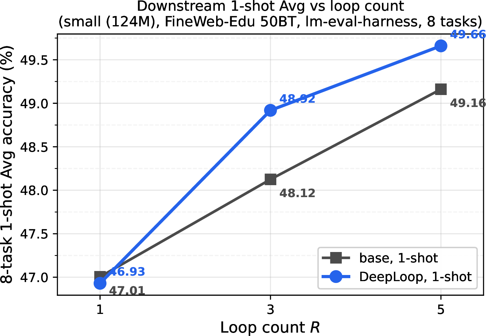
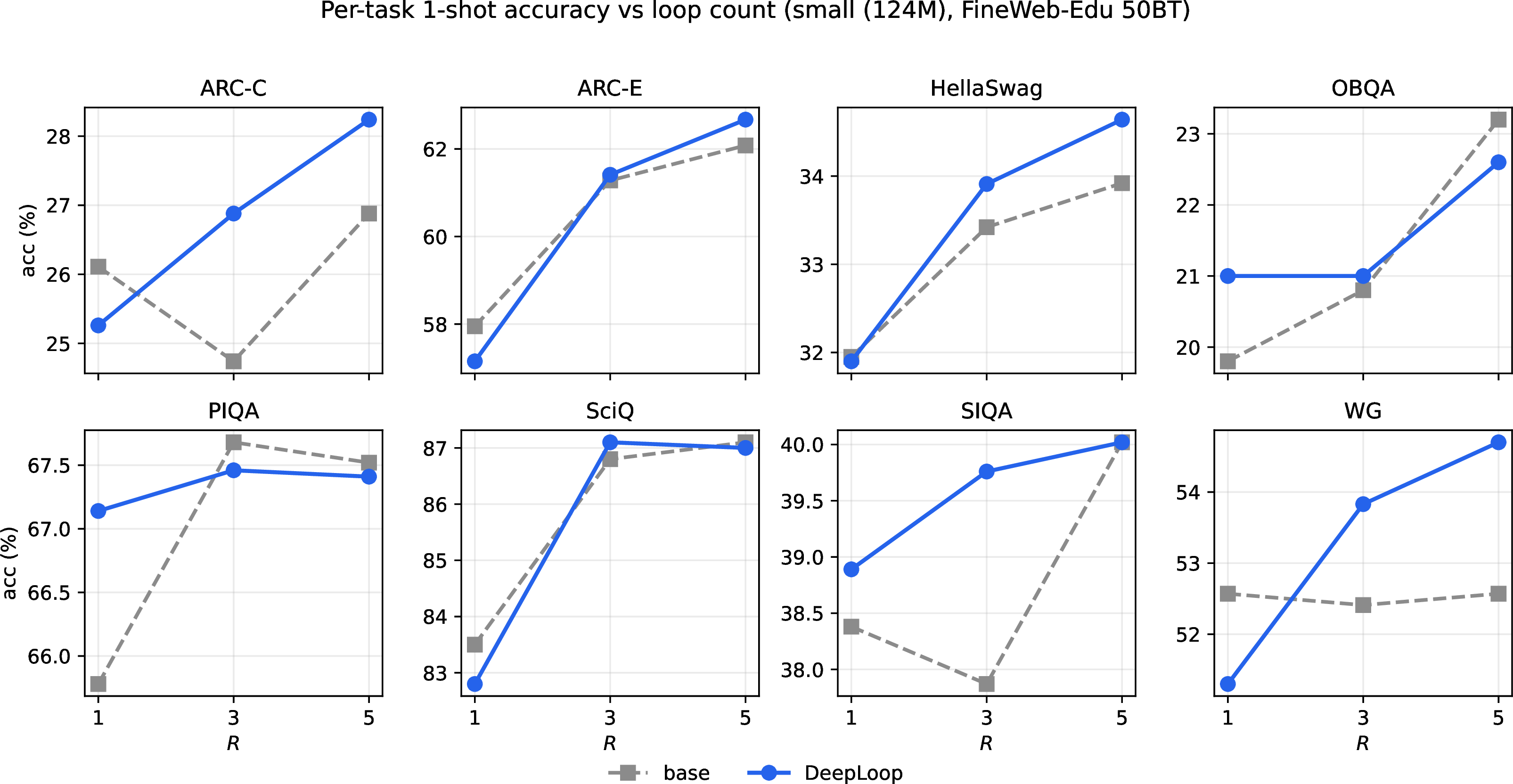
The two methods are within \(\pm 0.25\) points of each other at \(R{=}1\) on both shot settings, and DeepLoop has higher Avg at \(R{=}3\) (by \(+1.31\) and \(+0.79\) points on 0-shot and 1-shot respectively) and at \(R{=}5\) (by \(+0.15\) and \(+0.50\)). The headline small-scale cell is DeepLoop \(R{=}5\) 1-shot at \(49.66\,\%\). Against the same-\(R\) baseline (base \(R{=}5\) 1-shot, \(49.16\,\%\)), DeepLoop wins on four of the eight tasks (ARC-C, ARC-E, HellaSwag, WinoGrande), is within \(0.11\) points on three tasks (PIQA, SciQ, SIQA), and loses clearly only on OpenBookQA.
10 Empirical \(p\)-sweep at fixed loop count↩︎
Proposition [prop:exponent-threshold] predicts a sharp \(p{=}1/2\) training-stability threshold under the worst-case aligned regime. We test this prediction directly with a single-axis sweep over the exponent \(p\) at fixed \(R{=}3\) on the GPT-2 small backbone. All other ingredients, tied embeddings, input-embedding RMSNorm, FineWeb-Edu 50BT data pipeline, batch size, learning rate, and seed protocol, are identical to the runs in Table 1; only the residual scaling \(\alpha=(2N)^p\) and initialization gain \(\beta=(8N)^{-p}\) change. We run a grid of seven values, \(p\in\{0.30,0.35,0.40,0.45,0.50, 0.55,0.60\}\), with up to five seeds per value. Each cell is a 90-minute run on \(4\times\)H200 141 GB GPUs, which under our throughput reaches roughly \(2{,}700\) optimizer steps; we report validation loss at the common comparison checkpoint of step \(2000\) where available, and use the trailing-50-iter mean train loss as a surrogate for runs that do not reach a post-warmup validation step.
![Figure 6: Validation-loss snapshot at step 2000 on FineWeb-Edu 50BT for the GPT-2 small backbone, R{=}3, sweeping the residual-scaling exponent p\in\{0.30,\ldots,0.60\}. Each marker is one seed. Red crosses are seeds that never escape the unigram-frequency floor (\approx 7.67 nats); blue circles are seeds that train; the blue line connects the per-p trained-seed mean. Below p{=}0.45 all seeds diverge; at p{=}0.45 the boundary is crossed (some seeds train, some do not); at p\ge 0.50 training is reliable. The empirical phase boundary lines up with the Proposition [prop:exponent-threshold] prediction of p{=}1/2. Conditional on convergence, larger p gives a slightly higher loss (less aggressive learning), so p{=}1/2 is also the smallest p that is reliably stable, supporting it as the default DeepLoop choice.](/article/2607.13491/figures/p_sweep.png "fig:")
The picture in Figure 6 is consistent with the analysis. First, no seed at \(p\in\{0.30,0.35,0.40\}\) ever escapes the unigram floor: these clearly sub-threshold runs reproduce the divergence that Proposition [prop:exponent-threshold] predicts under the aligned worst case. Second, among seeds that do train, the mean validation loss at the same step rises monotonically as \(p\) increases across the boundary (\(3.70\) at \(p{=}0.45\), \(3.73\) at \(p{=}0.50\), \(3.76\) at \(p{=}0.55\), \(3.80\) at \(p{=}0.60\)), confirming that more aggressive scaling (smaller \(p\)) delivers a stronger learning signal whenever it does not destabilize training. Putting these two observations together: \(p{=}1/2\) is the smallest exponent that is reliably stable across seeds in this regime. We adopt it as the DeepLoop default for that reason. Sub-threshold choices \(p\in[0.45,0.50)\) produce lower trained-seed mean loss when they do train, but with \(\geq 1/3\) of seeds failing to leave the unigram floor before step \(2000\), they are not safe defaults.
The \(p\)-sweep is small in scope: it is at one scale (GPT-2 small), one loop depth (\(R{=}3\)), and one optimizer-step budget. Whether the same boundary at \(p{=}1/2\) applies at larger \(K\), at different normalization placements, or at substantially longer training, is left to future work and discussed in the Limitations paragraph (§6).
11 Compute resources↩︎
All experiments were run on NVIDIA H200 141 GB GPUs in a SLURM cluster. GPT-2 small cells use \(4\times\)H200, and GPT-2 medium cells use \(8\times\)H200. Per-cell wall-clock time is read from the corresponding WandB run records; aggregate GPU-hours below are rounded to the nearest hundred.
11.0.0.1 Per-cell cost.
Wall-clock time scales roughly linearly with the loop count \(R\):
| \(R{=}1\) | \(R{=}3\) | \(R{=}5\) | \(R{=}7\) | |
|---|---|---|---|---|
| Small wall-clock (h) | \(9\) | \(22\) | \(35\) | \(50\) |
| Small GPU-hours / cell | \(37\) | \(90\) | \(145\) | \(200\) |
| Medium wall-clock (h) | \(12\) | \(32\) | \(52\) | \(77\) |
| Medium GPU-hours / cell | \(95\) | \(260\) | \(420\) | \(620\) |
11.0.0.2 Aggregate cost.
The reported FineWeb-Edu language-modeling matrix (Tables 1 and 2: 16 cells \(\{\)base, DeepLoop\(\}\times\{\)small, medium\(\}\times R\in\{1,3,5,7\}\)) totals approximately \(\mathbf{3{,}700}\) H200 GPU-hours. Exploratory experiments not included in the main paper, a range of optimization-related variants and additional benchmark sweeps we evaluated during the development of the method and ultimately did not report, add approximately \(\mathbf{7{,}000}\) GPU-hours.
The total project compute is therefore approximately \(\mathbf{10{,}700}\) H200 GPU-hours.