¹

²

1 Introduction↩︎

Quantum process tomography is the task of learning an unknown quantum channel from query access, which serves as the key subroutine for calibration, verification, characterization, and certification across various quantum platforms [1]–[19]. The problem is formulated as: given queries to an unknown underlying quantum channel [20], output a classical description of a channel that is close to the actual channel in diamond norm, which captures the worst-case distinguishability of two processes where the user of the process may choose an arbitrary input state, attach an arbitrary reference system, and perform an arbitrary final measurement [12]–[16].

An essential task in this problem is to understand the role of quantum memory. A coherent process tomography protocol can preserve quantum systems across different uses of the unknown channel and is able to finally perform a joint quantum operation or measurement on all retained systems. An incoherent protocol, by contrast, uses the unknown channel one time at a time, measures immediately after each use, and stores only a classical transcript between different rounds. The incoherent protocol may still be adaptive: after observing the previous outcomes, it may choose a new input state, a new measurement, and even a fresh ancilla for the next channel use. This distinction is already known to be essential and is well-understood in quantum state tomography. For learning an arbitrary \(d\)-dimensional quantum state in trace distance, coherent collective measurements achieve the optimal sample complexity \(\Theta(d^2)\) while any incoherent single-copy measurement protocol requires \(\Theta(d^3)\) even when the measurements are chosen adaptively [18], [21]–[23]. This result separated two resources that are often conflated: adaptivity, the ability to choose later experiments based on earlier classical data, and coherence, the ability to keep quantum systems coherent across different copies. A more recent result even provides a smooth tradeoff between sample complexity and the number of copies on which each measurement is able to perform jointly [24]. For structured channels like Pauli channels, it is shown that entanglement and quantum memory can also lead to exponential separations in the number of queries [25]–[31].

However, the analogous question for quantum processes learning has remained more subtle for general channels with \(d_{\mathrm{in}}\) input and \(d_{\mathrm{out}}\) output dimensions. A general channel has a normalized Choi operator on a Hilbert space of \(d_{\mathrm{in}}d_{\mathrm{out}}\) dimensions [20]. However, the operational error in channel tomography is the diamond norm rather than the Choi trace norm in state tomography, which prevents a direct transfer of state-tomography bounds. Previous projected least-squares process tomography protocols gave rigorous incoherent upper bounds of \(\widetilde{O}(d_{\mathrm{in}}^3d_{\mathrm{out}}^3/\varepsilon^2)\) for achieving \(\varepsilon\)-accuracy in diamond norm, which includes logarithmic factors [32], [33], and proved a matching lower bound \(\Omega(d_{\mathrm{in}}^3d_{\mathrm{out}}^3/\varepsilon^2)\) only for non-adaptive incoherent measurements [33]. On the other hand, recent coherent protocols enable full process tomography in diamond norm with \(\Theta(d_{\mathrm{in}}^2d_{\mathrm{out}}^2/\varepsilon^2)\) queries [19], [34]. These coherent protocols establish the best possible scaling when quantum memory is allowed, leaving open whether classical adaptivity could reduce the sample complexity without quantum memory.

This work resolves this question by giving a negative answer. We prove that every adaptive incoherent protocol for learning an arbitrary channel with \(d_{\mathrm{in}}\) input and \(d_{\mathrm{out}}\) output dimensions up to \(\varepsilon\) accuracy in diamond norm requires \(\Omega(d_{\mathrm{in}}^3d_{\mathrm{out}}^3/\varepsilon^2)\) queries. The lower bound holds for any incoherent protocol with arbitrary classical adaptivity, arbitrary outcome-dependent measurements, and interaction with arbitrary fresh ancilla systems within each round. Our results also generalize the optimal sample-complexity bounds for single-copy state tomography: when \(d_{\mathrm{in}}=1\), channels reduce to states, and our lower and upper bounds recover the corresponding \(\Theta(d_{\mathrm{out}}^3/\varepsilon^2)\) scaling [23], [35].

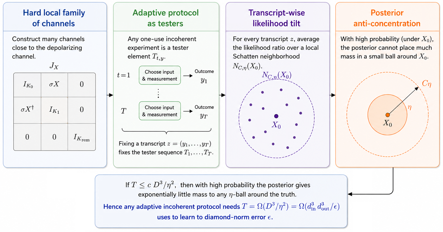
The proof follows the same high-level philosophy as the posterior-tilt method developed for adaptive incoherent state tomography [23], but the channel setting requires several new ingredients. First, we construct a local family of channels around the completely depolarizing channel by slightly perturbing the normalized Choi operator in off-diagonal blocks. Second, we represent each individual query in an adaptive incoherent protocol by a one-slot tester acting on the Choi operator using the standard tester and quantum-comb formalism [36], [37]. After conditioning on a full transcript, the adaptive choices of the protocol become a deterministic sequence of tester elements. Third, for every such fixed transcript, we prove a likelihood tilt bound over a local Schatten neighborhood of the true channel, which shows that the posterior cannot concentrate inside the Choi trace ball that would be forced by a diamond-norm accurate estimator with \(o(d_{\mathrm{in}}^3d_{\mathrm{out}}^3/\varepsilon^2)\) queries. The resulting posterior anti-concentration contradicts uniform successful tomography and yields the claimed result.

We complement the lower bound with a non-adaptive, ancilla-free incoherent protocol using \(O(d_{\mathrm{in}}^3d_{\mathrm{out}}^3/\varepsilon^2)\) queries, which removes the logarithmic factor from the previously best incoherent process tomography guarantees [32], [33]. Importantly, the protocol we consider remains the same as the previous work, while we carried out a refined concentration analysis in the same spirit of the incoherent state tomography work [35]: instead of applying a direct matrix-concentration bound that pays a logarithmic overhead, we control each fixed quadratic form by scalar Bernstein concentration and then use a constant-radius net of the unit sphere. This gives an operator-norm guarantee strong enough to imply the desired diamond-norm error without the logarithmic factor. Together with the coherent upper and lower bounds, our result gives a strict quantum-memory separation for full process tomography between \(\Theta(d_{\mathrm{in}}^2d_{\mathrm{out}}^2/\varepsilon^2)\) for coherent protocols and \(\Theta(d_{\mathrm{in}}^3d_{\mathrm{out}}^3/\varepsilon^2)\) for incoherent protocols.

2 Preliminaries↩︎

In this section, we introduce the basic notation and conventions. All Hilbert spaces considered in this work are finite-dimensional. The unknown channel maps \(\mathcal{L}(A)\) to \(\mathcal{L}(B)\), where \(A\simeq\mathbb{C}^{d_{\mathrm{in}}}\) and \(B\simeq\mathbb{C}^{d_{\mathrm{out}}}\). We write \(D:=d_{\mathrm{in}}d_{\mathrm{out}}\). For a Hilbert space \(H\), let \(\mathcal{L}(H)\) denote the linear operators on \(H\) and let \(\mathcal{D}(H)\) denote the density operators. Schatten norms are denoted by \(\left\|\cdot\right\|_1\), \(\left\|\cdot\right\|_2\), and \(\left\|\cdot\right\|_\infty\).

2.1 Choi convention↩︎

Fix a computational basis \(\{\ket{i}\}_{i=1}^{d_{\mathrm{in}}}\) of \(A\), and let \(A'\simeq A\) be a reference copy with the same basis. Define \[\ket{\Omega}_{A'A}:=\frac{1}{\sqrt{d_{\mathrm{in}}}}\sum_{i=1}^{d_{\mathrm{in}}}\ket{i}_{A'}\ket{i}_{A}.\] For a linear map \(\Phi:\mathcal{L}(A)\tilde{o}\mathcal{L}(B)\), we use the Choi characterization of completely positive trace-preserving maps in normalized form [15], [20] \[J_\Phi:=(\operatorname{id}_{A'}\otimes\Phi)(|\Omega\rangle\!\langle \Omega|)=\frac{1}{d_{\mathrm{in}}}\sum_{i,j=1}^{d_{\mathrm{in}}}\ketbra{i}{j}_{A'}\otimes\Phi(\ketbra{i}{j}_{A}).\] After defining \(J_\Phi\), we identify \(A'\) with \(A\) and regard \(J_\Phi\in\mathcal{L}(A\otimes B)\). All transposes are taken in the computational basis fixed above. With this normalization, \(\Phi\) is a quantum channel if and only if \[\require{physics} J_\Phi\ge0,\qquad \Tr_B J_\Phi=\frac{I_A}{d_{\mathrm{in}}}.\] We also use the diamond norm \(\left\|\cdot\right\|_\diamond\) and the elementary implication \[\left\|J_\Phi-J_\Psi\right\|_1\le\left\|\Phi-\Psi\right\|_\diamond\] for any linear maps \(\Phi,\Psi:\mathcal{L}(A)\tilde{o}\mathcal{L}(B)\).

2.2 Adaptive incoherent protocols↩︎

An adaptive incoherent protocol queries the unknown channel once at a time, makes a measurement, and stores only classical information between different measurements. We consider a protocol with \(T\) rounds of measurements. At round \(t\in\{1,\ldots,T\}\), after observing a classical history \(h_{t-1}=(y_1,\ldots,y_{t-1})\), the learner chooses an ancilla \(R_t\), an input state \(\rho_{h_{t-1}}\in\mathcal{D}(R_t\otimes A)\), and a discrete POVM \(\{M_{h_{t-1},y}\}_{y\in\mathcal{Y}_{h_{t-1}}}\) on \(R_t\otimes B\). Throughout the main proof, the outcome set \(\mathcal{Y}_{h_{t-1}}\) is taken to be finite or countably infinite. The channel is applied once to the ancillary register \(A\), the POVM is measured immediately, and the resulting outcome \(Y_t\) is appended to the transcript. We only allow classical adaptivity and processing among different rounds of measurements.

The full transcript of such a protocol is given by \(Z:=(Y_1,\ldots,Y_T)\), and the estimator \(\widehat{\Phi}\) is a function of \(Z\). In particular, \(\widehat{\Phi}\) need not be a channel. Randomized protocols are handled by conditioning on the private random seed. Consequently, it suffices to prove the lower bound for deterministic protocols and then average over the seed.

The restriction to discrete outcomes is only a notational simplification to make the transcript likelihoods point probabilities, and thus all sums over outcomes and transcripts are countable. The same results extend to arbitrary standard Borel outcome spaces by replacing point probabilities with Radon-Nikodym derivatives. We provide the corresponding measure-theoretic formulation in Appendix 12.

2.3 Single-round testers↩︎

A single incoherent use of a channel can be written in tester form, the one-slot case of the quantum strategy or comb formalism [36], [37]. A discrete single-round tester is a family of positive operators \[\{T_y\}_{y\in\mathcal{Y}},\qquad T_y\in\mathcal{L}(A\otimes B),\] such that, for some \(\tau\in\mathcal{D}(A)\), \[\sum_{y\in\mathcal{Y}}T_y=\tau^\top\otimes I_B .\] When the tested channel is \(\Phi\), the outcome probabilities are \[\require{physics} p_\Phi(y)=d_{\mathrm{in}}\,\Tr(T_yJ_\Phi).\]

In Section 4.1, we prove the representation lemma showing that every single round of a potentially adaptive protocol with incoherent measurements induces such a tester. Thus, along any fixed transcript \(z=(y_1,\ldots,y_T)\) of an adaptive protocol, the operators used in the likelihood ratio are deterministic: \[T_t(z):=T_{y_{<t},y_t},\qquad y_{<t}:=(y_1,\ldots,y_{t-1}).\]

2.4 Bayesian notation↩︎

For a channel family parametrized by \(\{\Phi_\theta:\theta\in\Theta\}\) and a fixed deterministic protocol, let \(P_\theta\) be the induced probability distribution over the transcript \(Z\). If \(\mu\) is a prior on \(\Theta\), the prior predictive distribution is \[P_\mu(z):=\int_\Theta P_\theta(z)\,d\mu(\theta).\] For every transcript \(z\) with \(P_\mu(z)>0\), the posterior is \[\nu_z(A):=\frac{\int_A P_\theta(z)\,d\mu(\theta)}{\int_\Theta P_\theta(z)\,d\mu(\theta)},\qquad A\subseteq\Theta.\] When a reference parameter \(\theta_0\) has common transcript support with all parameters under consideration, we also write \[R_\theta^{\theta_0}(z):=\frac{P_\theta(z)}{P_{\theta_0}(z)}\] and express the posterior as \[\nu_z(A)=\frac{\int_A R_\theta^{\theta_0}(z)\,d\mu(\theta)}{\int_\Theta R_\theta^{\theta_0}(z)\,d\mu(\theta)}.\]

3 Main results↩︎

Our main result is a lower bound for learning an arbitrary quantum channel in diamond norm for any adaptive incoherent process tomography protocol. The protocol may choose its input state and measurement at each round as an arbitrary function of the previous classical outcomes, and use an unbounded-size ancilla register within each round. As the measurements are assumed incoherent, only classical adaptivity is allowed among different measurement rounds. The proof strategy is summarized in Fig. 1.

We emphasize that the lower bound applies to any incoherent strategy with classical adaptivity between rounds, arbitrary ancilla-assisted inputs within each round, and arbitrary outcome-dependent measurements. Theorem 1 is complemented by a non-adaptive ancilla-free upper bound \(O({d_{\mathrm{in}}^3d_{\mathrm{out}}^3}/{\varepsilon^2})\), derived in Section 5. The upper bound is based on previously introduced algorithm, and our contribution is to remove the logarithmic factor in the previously best known bound [32], [33]. Therefore, for unknown channels \(\Phi:\mathcal{L}(\mathbb{C}^{d_{\mathrm{in}}})\tilde{o}\mathcal{L}(\mathbb{C}^{d_{\mathrm{out}}})\), the optimal query complexity for diamond-norm incoherent process tomography is \[\Theta\left(\frac{d_{\mathrm{in}}^3d_{\mathrm{out}}^3}{\varepsilon^2}\right).\]

Since incoherent protocols are allowed arbitrary classical adaptivity, any remaining gap between incoherent and coherent tomography must instead come from the ability to preserve and jointly process quantum information across channel uses. Coherent process tomography protocols that may retain and jointly process quantum information across channel uses achieve the optimal query complexity \[\Theta\left(\frac{d_{\mathrm{in}}^2d_{\mathrm{out}}^2}{\varepsilon^2}\right)\] for the same task [19], [34]. Hence, quantum memory improves the sample complexity by a factor of \(R=\Theta(d_{\mathrm{in}}d_{\mathrm{out}})\) over any fully adaptive incoherent strategy.

4 Lower bound↩︎

This section formalizes the proof sketch presented in Fig. 1, while deferring most of the fully detailed proofs to the appendix. We first reduce each single-round experiment to a tester acting on the Choi operator. We then construct the hard local family of channels and record the geometric properties of the prior. The key technical subroutine is the transcript-wise adaptive test tilt lemma, which controls likelihood ratios uniformly along a fixed adaptive transcript. Finally, we convert this likelihood control into posterior anti-concentration and use it to prove Theorem 1. After completing the lower-bound proof, Section 5 states the matching non-adaptive incoherent upper bound.

4.1 Single-round tester formalism↩︎

The first step is to separate the physical implementation of a single incoherent experiment from its statistical effect on the unknown channel. At a fixed history of an adaptive protocol, the learner has chosen an ancilla-assisted input state and a measurement on the output. The following lemma shows that, as a function of the channel, this entire single-round experiment is equivalently described by a collection of positive operators acting on the Choi space \(A\otimes B\).

The proof of Lemma 1 is given by a standard purification-and-vectorization argument and is provided in Appendix 7. The key point is that the operators \(T_y\) depend only on the chosen experiment instead of the unknown channel. All dependence on \(\Phi\) enters linearly through the normalized Choi operator \(J_\Phi\).

Applying Lemma 1 at each history of an adaptive incoherent protocol gives the following transcript-wise representation. If \(h=(y_1,\ldots,y_{t-1})\) is a possible history before round \(t\), then the input state and POVM chosen by the protocol at \(h\) induce tester elements \(\{T_{h,y}\}_{y\in\mathcal{Y}_h}\) satisfying \[\sum_{y\in\mathcal{Y}_h}T_{h,y}=\tau_h^\top\otimes I_B\] for some \(\tau_h\in\mathcal{D}(A)\), and \[\require{physics} \mathbb{P}_\Phi[Y_t=y\mid h]=d_{\mathrm{in}}\,\Tr(T_{h,y}J_\Phi).\] Consequently, once a full transcript \(z=(y_1,\ldots,y_T)\) is fixed, the adaptive choices along that transcript become deterministic. We write \[T_t(z):=T_{y_{<t},y_t},\qquad y_{<t}:=(y_1,\ldots,y_{t-1}).\] Thus, for any reference channel \(\Phi_0\) and any transcript \(z\) with \(P_{\Phi_0}(z)>0\), the likelihood ratio factors as \[\require{physics} \frac{P_\Phi(z)}{P_{\Phi_0}(z)}=\prod_{t=1}^T\frac{\Tr(T_t(z)J_\Phi)}{\Tr(T_t(z)J_{\Phi_0})}. \label{eq:transcript-likelihood-ratio}\tag{1}\] The factors \(d_{\mathrm{in}}\) cancel in the ratio. Eq. 1 is the formal mechanism by which we handle adaptivity. Although the protocol may choose each experiment as an arbitrary function of the past, conditioning on a transcript freezes those choices. The lower bound will therefore control adaptive protocols by proving a likelihood-ratio estimate that holds for every deterministic sequence of tester elements arising along a transcript.

4.2 Construction of the hard channel family↩︎

We now construct the local family of channels used in our main results. The family is centered at the completely depolarizing channel with the normalized Choi operator \[\require{physics} \Phi_{\mathrm{dep}}(\rho)=\Tr(\rho)\frac{I_B}{d_{\mathrm{out}}},\quad J_{\mathrm{dep}}=\frac{I_{AB}}{D}.\]

The perturbations are chosen so that they preserve the trace-preserving constraint exactly, while creating a high-dimensional set of locally separated channels. Fix a universal constant \(0<\sigma\le 10^{-3}\), we decompose the output space as \[\begin{align} B=B_0\oplus B_1&\oplus B_{\mathrm{rem}},\\ \dim B_0=\dim B_1=&\;s:=\left\lfloor\frac{d_{\mathrm{out}}}{2}\right\rfloor. \end{align}\] Set \[\begin{align} &K_0:=A\otimes B_0,\qquad K_1:=A\otimes B_1,\\ &r:=\dim K_0=\dim K_1=d_{\mathrm{in}}s. \end{align}\] Since \(d_{\mathrm{out}}\ge2\), this auxiliary dimension satisfies \[\frac{D}{3}\le r\le\frac{D}{2}. \label{eq:r-dimension-comparison}\tag{2}\] After fixing orthonormal bases of \(K_0\) and \(K_1\), we identify both spaces with \(\mathbb{C}^r\). For \(X\in\mathbb{C}^{r\times r}\), interpreted as an operator \(K_1\tilde{o}K_0\), define the Hermitian off-diagonal block operator \[E(X):=\begin{pmatrix} 0 & X\\ X^\dagger & 0 \end{pmatrix}\] on \(K_0\oplus K_1\), extended by zero on \(A\otimes B_{\mathrm{rem}}\). The defining feature of this embedding is that the perturbation is invisible to the partial trace over \(B\). Thus it preserves the affine constraint \(\require{physics} \Tr_BJ=I_A/d_{\mathrm{in}}\) for Choi operators of channels.

The proof is a direct block-matrix computation and is deferred to Appendix 8.

We are now ready to define the local family. Let \[\begin{align} S:=\{X\in\mathbb{C}^{r\times r}:\left\|X\right\|_\infty\le4\},\\ G:=\{X\in\mathbb{C}^{r\times r}:\left\|X\right\|_\infty\le3\}. \end{align}\] For \(X\in S\) and \(\sigma\geq 0\), define \[J_X:=\frac{I_{AB}}{D}+\frac{\sigma}{D}E(X). \label{eq:hard-family-choi}\tag{3}\]

Therefore, the hard family is a local perturbation of the depolarizing channel inside the full-rank part of the channel set. The set \(G\) will be the “regular” part of the prior: under the prior that we introduce in the subsequent Section 4.3, we will sample an \(X\) with an overwhelming probability in \(G\). The larger set \(S\) gives a slightly thicker support on which the channels remain uniformly full rank.

Finally, the parametrization converts Schatten trace distance in the matrix parameter \(X\) exactly into Choi trace distance.

Consequently, a Choi trace ball of radius \(\eta\) around \(J_{X_0}\) corresponds to a Schatten-\(1\) ball in the local parameter \(W\) of radius \[L_\eta:=\frac{\eta D}{2\sigma}. \label{eq:L-eta-definition}\tag{4}\] This exact conversion is the reason for using the off-diagonal embedding \(E(X)\): it lets us phrase posterior concentration around the true channel as a local volume question in the matrix space \(\mathbb{C}^{r\times r}\), where \(r=\Theta(D)\).

4.3 Prior regularity and local geometry↩︎

We next put a prior on the hard family and present the local geometric facts used in the posterior argument. The prior is a truncated complex Ginibre measure on the matrix parameter \(X\), which has two useful features: typical draws lie in the well-conditioned set \(G\), and the prior density is sufficiently regular on its support \(S\).

Quantitatively, let \(\mu\) be the probability measure on \(S=\{X\in\mathbb{C}^{r\times r}:\left\|X\right\|_\infty\le4\}\) with density \[f_\mu(X)=\frac{1}{Z}\mathrm{exp}(-r\left\|X\right\|_2^2)\mathbf{1}_S(X)\] with respect to Lebesgue measure on \(\mathbb{C}^{r\times r}\simeq\mathbb{R}^{2r^2}\), where \[Z=\int_S \mathrm{exp}(-r\left\|X\right\|_2^2)\,dX .\] Equivalently, \(\mu\) is the complex Ginibre distribution with independent entries of density \[z\mapsto \frac{r}{\pi}e^{-r|z|^2},\qquad z\in\mathbb{C},\] conditioned on \(\left\|X\right\|_\infty\le4\).

The proof, given in Appendix 9, uses only the standard operator-norm tail bound for complex Ginibre matrices. The first conclusion says that a draw from the prior is regular with overwhelming probability. The second is a deliberately crude density-ratio bound costing only \(\mathrm{exp}(O(D^2))\), which is of the same order as the dimension of the local parameter space and is harmless in the final volume comparison.

We now define the local neighborhoods used to test posterior concentration. For \(X_0\in S\) and \(\eta>0\), let \[B_\eta(X_0):=\{X\in S:\left\|J_X-J_{X_0}\right\|_1\le\eta\}\] be the set of matrices \(X\) in the hard family whose Choi operators are within trace-norm distance \(\eta\) of \(J_{X_0}\). By Lemma 4, \[B_\eta(X_0)=\{X_0+W\in S:\left\|W\right\|_1\le L_\eta\},\;L_\eta:=\frac{\eta D}{2\sigma}. \label{eq:Beta-Leta}\tag{5}\] We also write \[\widetilde{B}_\eta(X_0):=\{X_0+W:\left\|W\right\|_1\le L_\eta\}\] for the unrestricted translate, so that \[\operatorname{vol}(\widetilde{B}_\eta(X_0))=\operatorname{vol}\{W:\left\|W\right\|_1\le L_\eta\}.\] The posterior anti-concentration argument will compare the small ball \(B_\eta(X_0)\) with a larger, regularized neighborhood. For \(C>1\), we define \[N_{C,\eta}:=\left\{W\in\mathbb{C}^{r\times r}:\left\|W\right\|_1\le C L_\eta,\;\left\|W\right\|_\infty\le\frac{C L_\eta}{4r}\right\}. \label{eq:NCeta-definition}\tag{6}\] The condition \(\left\|W\right\|_1\le C L_\eta\) places \(X_0+N_{C,\eta}\) inside the Choi trace ball \(B_{C\eta}(X_0)\), while the additional operator-norm constraint ensures that every perturbation is pointwise small enough for the likelihood-ratio estimates below.

Thus, for regular centers \(X_0\in G\), the translated set \(X_0+N_{C,\eta}\) remains inside the support of the prior. In particular, under the same condition on \(\eta\), \[X_0+N_{C,\eta}\subseteq B_{C\eta}(X_0). \label{eq:NCeta-contained-large-ball}\tag{7}\]

The final geometry on the input is that the regularized enlargement \(N_{C,\eta}\) has exponentially larger volume than the original trace ball once \(C\) is chosen large enough, which results in the entropy source for the anti-concentration argument.

The proof of Lemma 7, deferred to Appendix 9, uses the standard volume-radius asymptotic approximation for complex Schatten balls [38]. The exponent \(2r^2\) is the dimension of \(\mathbb{C}^{r\times r}\). Since \(r=\Theta(D)\), the volume gain from enlarging by a constant factor is of order \(\mathrm{exp}(\Theta(D^2))\), which will dominate the prior density-ratio loss in Eq. ?? and the likelihood loss controlled in the next section.

4.4 The transcript-wise adaptive tester tilt lemma↩︎

We now state the main technical estimate that handles adaptivity. A standard Bayesian lower bound might try to control the information gained in each round. However, such a single-step bound is not sufficient here by itself, because an adaptive protocol may choose later testers that are highly tuned to the posterior produced by earlier outcomes. We observe that, once the transcript is fixed, the adaptive protocol becomes a deterministic sequence of tester elements, as in Eq. 1 . The lemma below controls the average likelihood ratio over a local Schatten neighborhood for every such frozen transcript.

Fixing a regular center \(X_0\in G\) and a perturbation \(W\in N_{C,\eta}\), we write \[\Delta_W:=J_{X_0+W}-J_{X_0}=\frac{\sigma}{D}E(W).\] The assumptions in the next lemma ensure that by Lemma 6, \(X_0+W\) remains in the support \(S\) of the hard family, and that each single-step likelihood perturbation is uniformly small enough for quadratic logarithmic estimates to apply.

Lemma 8 shows that, averaged over the symmetric neighborhood \(N_{C,\eta}\), no fixed adaptive transcript can suppress the likelihood by more than \(\mathrm{exp}(O(C^2\eta^2T/D))\). The factor \(1/D\) per query to channel is the key quantitative gain. In the posterior argument, it will be compared against the volume growth \[\frac{\operatorname{vol}(N_{C,\eta})}{\operatorname{vol}\{W:\left\|W\right\|_1\le L_\eta\}}\ge C^{2r^2}e^{-c_{\mathrm{vol}}r^2},\] which is exponential in \(r^2=\Theta(D^2)\). Balancing these two terms gives the lower-bound asymptotic scaling \[T=\Omega\left(\frac{D^3}{\eta^2}\right).\]

We prove Lemma 8 in Appendix 10. The proof has three ingredients. First, the operator-norm constraint in \(N_{C,\eta}\) makes every single-step likelihood ratio close to one. Second, the off-diagonal embedding \(E(W)\) reduces each linear fluctuation to a matrix inner product \(\require{physics} \Tr(B_t^\dagger W)\) against the off-diagonal block of the tester. Third, the unitary invariance of \(N_{C,\eta}\) gives an isotropic covariance bound for \(W\), which yields a transcript-wise second-moment estimate. Jensen’s inequality then converts this second-moment control into the lower bound in Eq. ?? .

4.5 Posterior anti-concentration↩︎

We now convert the transcript-wise tilt estimate into the main Bayesian statement used in the main result. For \(X\in S\), let \(P_X\) denote the law of the full transcript \(Z\) when the unknown channel is \(\Phi_X\). The first observation is that all channels in the hard family induce the same transcript support.

The proof is given in Appendix 11. It uses only the uniform full-rank lower bound in Eq. ?? : at any history, whether a single-step outcome has positive probability is determined only by whether the corresponding tester element is nonzero, and not by the choice of \(X\in S\).

Fixing \(X_0\in G\), for a transcript \(z\) in the common support, we define the likelihood ratio as \[R_X(z):=\frac{P_X(z)}{P_{X_0}(z)} .\] By Lemma 9, \(R_X(z)\) is positive and finite for all \(X\in S\) on this support. Moreover, \[\mathbb{E}_{Z\sim P_{X_0}}R_X(Z)=1 .\] Let \(X\sim\mu\) and, conditional on \(X\), let \(Z\sim P_X\). For every transcript \(z\) with positive prior predictive probability, we have \[P_\mu(z):=\int_S P_X(z)f_\mu(X)\,dX,\] the posterior is \[\nu_z(A):=\frac{\int_{A\cap S}P_X(z)f_\mu(X)\,dX}{\int_S P_X(z)f_\mu(X)\,dX},\quad A\subseteq S .\] Equivalently, for a fixed \(X_0\in G\) and a transcript \(z\) in the common support, \[\nu_z(A)=\frac{\int_{A\cap S}R_X(z)f_\mu(X)\,dX}{\int_S R_X(z)f_\mu(X)\,dX}.\]

The following lemma is the posterior anti-concentration statement, which indicates that, below the sample size \(D^3/\eta^2\), the posterior cannot assign substantial mass to a Choi trace ball of radius \(\eta\) around the true channel, with high probability over transcripts generated by that true channel.

The proof of Lemma 10 is deferred to Appendix 11. The argument compares two posterior masses around the same center \(X_0\). First, a Markov inequality shows that the unweighted likelihood integral over the small ball \(B_\eta(X_0)\) is rarely much larger than its volume. Second, the transcript-wise tilt lemma lower bounds the likelihood integral over the larger regularized neighborhood \(X_0+N_{C,\eta}\subseteq B_{C\eta}(X_0)\). The volume gain from \(N_{C,\eta}\) is exponential in \(r^2=\Theta(D^2)\), while the likelihood loss is at most of scaling \[\mathrm{exp}\left(O\left(\frac{\eta^2T}{D}\right)\right).\] Thus, when \(T\lesssim D^3/\eta^2\), the larger neighborhood has much more posterior mass than the smaller ball. Since the larger posterior mass is at most one, the smaller posterior mass must be exponentially small.

This anti-concentration lemma is the final building block of the proof for Theorem 1. In the next section, we show that any uniformly accurate estimator would force the posterior to place non-negligible mass in one such small ball, contradicting Eq. ?? .

4.6 Proof of the main theorem↩︎

We now assemble the preceding ingredients to prove Theorem 1.

5 A matching non-adaptive upper bound↩︎

In this section, we show that the scaling of Theorem 1 is tight up to a constant factor by deriving a matching upper bound. The construction builds on the covariant projected-least-squares approach to incoherent process tomography [32], [33], but replaces the direct matrix-concentration step by scalar concentration for fixed quadratic forms followed by a constant-radius covering argument. This removes the logarithmic factor in the previously best known upper bound.

The protocol and the proof of Theorem 2 are given in Appendix 13. The estimator is an unbiased single-query estimator of the normalized Choi operator. The key observation is that every fixed quadratic form has variance bounded by a universal constant. Scalar Bernstein concentration therefore gives a tail of order \(\mathrm{exp}(-\Omega(T\varepsilon^2/D^2))\) in each fixed direction. A constant-radius net of the unit sphere has cardinality \(\mathrm{exp}(O(D))\), and the resulting union bound requires only \(T=O(D^3/\varepsilon^2)\) queries.

6 Discussion↩︎

We have established that quantum process tomography exhibits a strict quantum memory advantage. In the model considered here, the learner may use arbitrary ancilla-assisted inputs within each channel query, perform arbitrary measurements after each use, carry out classical computation, and choose each future experiment as an arbitrary function of the entire previous transcript. The only forbidden resource is the ability to preserve quantum information across different uses of the unknown channel. Our main result shows that every such adaptive incoherent protocol requires \(\Omega\left(d_{\mathrm{in}}^3d_{\mathrm{out}}^3/\varepsilon^2\right)\) queries. Together with the non-adaptive ancilla-free upper bound in Theorem 2, this gives the optimal incoherent query complexity \[\Theta\left(\frac{d_{\mathrm{in}}^3d_{\mathrm{out}}^3}{\varepsilon^2}\right).\] For \(d_{\mathrm{in}}=1\), this recovers the optimal sample-complexity bounds for single-copy state tomography [23], [35]. Since coherent protocols achieve the optimal query complexity \(\Theta(d_{\rm in}^2d_{\rm out}^2/\varepsilon^2)\) [19], [34], our results isolate quantum memory as the resource responsible for the separation.

We expect the techniques developed here for proving lower bounds against adaptive incoherent protocols in general channel tomography to be useful more broadly. Many quantum learning settings share the same underlying structure: each round consists of a quantum experiment, but only a classical outcome is retained before the next experiment is chosen. Natural directions include extending our methods to structured families of channels, unitaries, and dynamical processes, such as fermionic linear-optical and bosonic Gaussian processes [39], [40], Pauli channels [29], and adaptive single-copy POVMs tomography [41].

Several other directions remain open. First, it would be interesting to characterize the intermediate regimes between fully incoherent and fully coherent process tomography, in analogy with recent memory tradeoffs for state and Pauli-channel learning [24], [26], [28]. In particular, how much quantum memory is required to obtain a nontrivial improvement over the optimal incoherent rate? A second direction is to determine the full query complexity of incoherent channel tomography as a function of the Kraus rank. Notably, adaptive lower bounds remain open even for bounded-rank state tomography [23]. Establishing corresponding lower bounds for low-Kraus-rank channels therefore appears to require overcoming difficulties that are already present in the simpler state-tomography setting. Finally, another important direction is to study process tomography with limited or noisy quantum memory, i.e., when only a limited number of coherent qubits can be stored across channel uses, and determine when this already suffices to obtain an advantage over incoherent protocols [30], [42].

Acknowledgments↩︎

We thank Richard Allen, Senrui Chen, Sitan Chen, Angus Lowe, and Angelos Pelecanos for helpful discussions. C.B.-P. and A.A.M. acknowledge the BMFTR (MUNIQC-Atoms, HYBRID, QuSol, Hybrid++), the DFG (CRC 183 and SPP 2514), the Quantum Flagship (Millenion, PasQuanS2), the Munich Quantum Valley, Berlin Quantum and the European Research Council (DebuQC) for financial support. A.A.M. further acknowledges support from a 2025 Google PhD Fellowship. W.G. is supported by NSF Grant CCF-2430375 and the Von Neumann Award from Harvard Computer Science. We acknowledge ChatGPT for assistance in discussing and refining proof ideas, as well as improving the presentation. The authors are solely responsible for the proofs and the results.

7 Proof of the single-round tester representation↩︎

8 Algebra of the hard channel family↩︎

We collect the elementary properties for the hard family introduced in Section 4.2. We first observe that, since \(s=\lfloor d_{\mathrm{out}}/2\rfloor\), \[r=d_{\mathrm{in}}s\le \frac{d_{\mathrm{in}}d_{\mathrm{out}}}{2}=\frac{D}{2}.\] For the lower bound, every integer \(m\ge2\) satisfies \(\lfloor\tfrac{m}{2}\rfloor\ge\tfrac{m}{3}\). Therefore, \[r=d_{\mathrm{in}}\left\lfloor\frac{d_{\mathrm{out}}}{2}\right\rfloor\ge\frac{d_{\mathrm{in}}d_{\mathrm{out}}}{3}=\frac{D}{3}.\] Given that \(\tfrac{D}{3}\le r\le\frac{D}{2}\), we now prove Lemma 2, Lemma 3, and Lemma 4.

9 Proofs for prior regularity and local geometry↩︎

10 Proof of the transcript-wise adaptive tester tilt lemma↩︎

11 Proofs for posterior anti-concentration↩︎

12 General outcome spaces↩︎

The main text is written for discrete outcome spaces in order to avoid measure-theoretic notation. We now record the standard-Borel formulation and explain why all proofs above extend without change.

Fix one round of an incoherent protocol at a history \(h\). Let \((\mathcal{Y}_h,\Sigma_h)\) be a standard Borel outcome space, \(\rho_h\in\mathcal{D}(R_h\otimes A)\) be the chosen input state, and let \(M_h:\Sigma_h\tilde{o}\mathcal{L}(R_h\otimes B)\) be a POVM. By the same purification-and-vectorization argument as in Lemma 1, there is a positive operator-valued measure and a state \(\tau_h\in\mathcal{D}(A)\) such that for every channel \(\Phi\), we have \[\require{physics} T_h:\Sigma_h\tilde{o}\mathcal{L}(A\otimes B),\qquad T_h(\mathcal{Y}_h)=\tau_h^\top\otimes I_B,\qquad \Pr_\Phi[Y_t\in E\mid h]=d_{\mathrm{in}}\,\Tr\left(T_h(E)J_\Phi\right),\quad E\in\Sigma_h .\] Since \(A\otimes B\) is finite-dimensional, the scalar measure \(\require{physics} \lambda_h(E):=\Tr T_h(E)\) dominates the operator-valued measure \(T_h\). Hence there exists a \(\lambda_h\)-measurable positive-operator-valued density \(y\mapsto T_h(y)\) such that \[T_h(E)=\int_E T_h(y)\,d\lambda_h(y).\] Consequently the conditional distribution of \(Y_t\), given \(h\), has density \[\require{physics} p_X(y\mid h)=d_{\mathrm{in}}\,\Tr\left(T_h(y)J_X\right)\] with respect to \(\lambda_h\), for every channel in the hard family.

The full-rank bound in Lemma 3 implies common conditional support. Indeed, for every \(X\in S\), we have \(J_X\succeq \tfrac{1-4\sigma}{D}I_{AB}\succ0\), and therefore \[p_X(y\mid h)>0\qquad\Longleftrightarrow\qquad T_h(y)\ne0.\] Thus the conditional support is independent of \(X\). We note that the adaptive protocol induces mutually absolutely continuous transcript laws on the standard-Borel transcript space. For a reference point \(X_0\in S\), the likelihood ratio is, for \(P_{X_0}\)-almost every transcript \(z=(y_1,\ldots,y_T)\), \[\require{physics} \frac{dP_X}{dP_{X_0}}(z)=\prod_{t=1}^T\frac{\Tr\left(T_t(z)J_X\right)}{\Tr\left(T_t(z)J_{X_0}\right)},\] where \(T_t(z)\) denotes the density of the tester at the outcome observed at round \(t\), along the history determined by \(z\).

All arguments in Sections 4.4 and 4.5 use only this product likelihood ratio, common support, positivity of the tester densities, and Markov inequalities. These ingredients hold exactly as above. Therefore, Theorem 1 and its corollaries extend from discrete outcome spaces to arbitrary standard Borel outcome spaces.

13 Proof of the incoherent upper bound↩︎

In this appendix, we prove Theorem 2, removing the logarithmic factors appearing in the previously established upper bounds for incoherent channel tomography [33], [35]. Our proof adapts the technique of Ref. [35], which gives an optimal upper bound without logarithmic overhead for incoherent state tomography, to the setting of quantum channels. Throughout, for a unit vector \(u\), write \(P_u:=|u\rangle\!\langle u|\). Let \(\mu_d\) denote normalized Haar measure on the unit sphere of \(\mathbb{C}^d\).

13.1 The estimator↩︎

Fix an integer \(T\ge1\). For each \(t\in\{1,\ldots,T\}\), independently perform the following experiment.

1. Sample a Haar-random unit vector \(v_t\in A\).

2. Prepare \(P_{v_t}\), apply \(\Phi\) once, and obtain the output state \(\Phi(P_{v_t})\).

3. Independently sample \(U_t\) from Haar measure on \(U(d_{\mathrm{out}})\) and measure \(\Phi(P_{v_t})\) in the orthonormal basis \(\{U_t\ket{j}\}_{j=1}^{d_{\mathrm{out}}}\). Let \(I_t\) be the observed outcome and set \(w_t:=U_t\ket{I_t}\).

4. Form the Hermitian random operator \[X_t:=\left((d_{\mathrm{in}}+1)P_{v_t}^{\top}-I_A\right)\otimes\left((d_{\mathrm{out}}+1)P_{w_t}-I_B\right). \label{eq:upper-Xt-definition}\tag{20}\]

Define the linear estimator \[L_T:=\frac{1}{T}\sum_{t=1}^T X_t. \label{eq:upper-LT-definition}\tag{21}\] Let \[\require{physics} \mathfrak C_{A\tilde{o}B}:=\left\{K\in\mathcal{L}(A\otimes B):K\ge0,\;\Tr_BK=\frac{I_A}{d_{\mathrm{in}}}\right\} \label{eq:upper-choi-feasible-set}\tag{22}\] be the set of normalized Choi operators of channels from \(A\) to \(B\), and choose \[\widetilde{J}\in\mathop{\mathrm{arg\,min}}_{K\in\mathfrak C_{A\tilde{o}B}}\left\|K-L_T\right\|_\infty. \label{eq:upper-projection-definition}\tag{23}\] Finally, return the unique channel \(\widetilde{\Phi}\) whose normalized Choi operator is \(\widetilde{J}\).

The minimizer in Eq. 23 exists. Indeed, \(\mathfrak C_{A\tilde{o}B}\) is closed, and every \(K\in\mathfrak C_{A\tilde{o}B}\) satisfies \(K\ge0\) and \(\require{physics} \Tr K=1\), hence \(\left\|K\right\|_\infty\le1\). Thus \(\mathfrak C_{A\tilde{o}B}\) is compact in finite dimension, and the objective in Eq. 23 is continuous. All vectors \(v_t\) and bases \(U_t\) may be sampled before the experiment begins. Each \(X_t\) uses exactly one query of \(\Phi\), each channel output is measured separately, and no ancillary system is used. The protocol is therefore non-adaptive, incoherent, and ancilla-free.

13.2 Haar moments and random-basis reconstruction↩︎

The following lemma is standard and has previously been used in the contexts of quantum state tomography and classical shadows [35], [45]. For completeness, we provide a self-contained proof with explicit constants.

13.3 Unbiasedness of the Choi estimator↩︎

13.4 Dimension-independent directional variance↩︎

13.5 Scalar concentration and a covering net↩︎

We recall the following standard form of Bernstein’s inequality; see, for example, Ref. [46]. For completeness, we include a self-contained proof that keeps track of the constants.

13.6 Projection and conversion to diamond norm↩︎

References↩︎

---

1. {c.bravo.prieto, a.mele}fu-berlin.de?↩︎

2. {c.bravo.prieto, a.mele}fu-berlin.de?↩︎