Ego-Dynamics-Augmented World Model for Autonomous Driving with Zero-Shot Cross-Chassis Adaptation
July 15, 2026
Abstract
World model (WM)-based reinforcement learning enables sample-efficient end-to-end autonomous driving learning by imagining long-horizon trajectories in latent space. However, most driving WMs operate on bird’s-eye-view (BEV) representations that are inherently egocentric: the transition between consecutive frames entangles the ego vehicle’s own motion with scene dynamics. As a result, the WM devotes significant capacity to recovering ego-motion from warped observations, at the cost of scene modeling fidelity and imagination accuracy. This work proposes DynaDreamer, a dynamics-augmented Dreamer-style reinforcement learning method to address this problem by augmenting the WM with an explicit ego-dynamics prior. A physics-informed ego-dynamics encoder-decoder extracts the ego-state history into a compact and identifiable context, which modulates a causal Transformer WM to condition both its prior and posterior latents. During imagination, the ego-dynamics predictor propagates this context forward to keep the ego-dynamics prior synchronized with the rollout. An information-theoretic analysis shows that conditioning on this context reduces both the predictive entropy of the observation transition and the prior–posterior Kullback–Leibler divergence, confining the WM’s modeling burden to the scene dynamics beyond ego-motion. An additional benefit is zero-shot cross-chassis adaptation: the ego-dynamics context depends on identifiable chassis parameters, so that a vehicle with previously unseen dynamic characteristics can adapt the WM to the new chassis without retraining. Experiments demonstrate that DynaDreamer improves task success rates over the strongest baseline by 28% and 61% in urban and highway driving scenarios, respectively, with the advantage rising to 73% when extrapolating to unseen chassis.
World model, model-based reinforcement learning, vehicle dynamics, autonomous driving.
1 Introduction↩︎
End-to-end autonomous driving has emerged as a prominent paradigm, in which a single model maps raw sensor inputs directly to planning outputs such as waypoints or low-level control commands [1]. A prevailing architecture fuses surround-view camera images into a BEV representation that provides a unified metric canvas, decoupling planning from camera-specific geometry and enabling joint perception–planning optimization [2]. Within this BEV-centric paradigm, imitation learning (IL) has become the dominant formulation owing to the abundance of human driving demonstrations [3], yet it suffers from open-loop causal confusion and poor generalization to out-of-distribution scenarios. Reinforcement learning (RL) restores closed-loop competence through environmental feedback [4], but remains sample-inefficient when operating on high-dimensional observations. World models alleviate this bottleneck by learning compact latent dynamics in which imagined trajectories can be rolled out without real environment interaction, driving rapid progress in WM-based RL for autonomous driving [5].
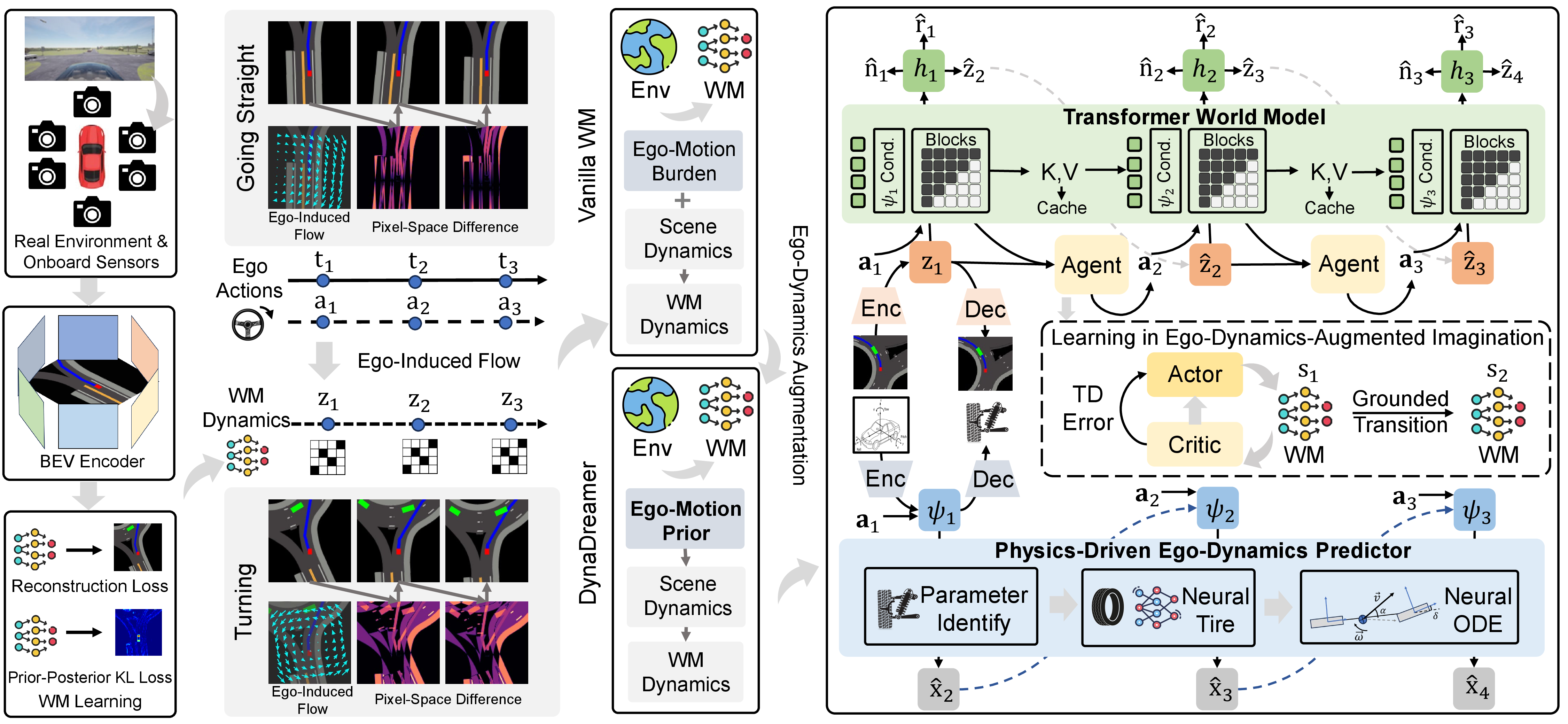
The quality of a WM-based RL policy is fundamentally bounded by the modeling fidelity of its WM. In the BEV setting, this fidelity faces a unique challenge: the ego vehicle is fixed at the image center, and the scene is rendered in the ego-centric frame. The change between consecutive frames is therefore an egocentric flow field that superimposes two distinct sources: the ego-induced flow from the viewpoint change and the object-induced flow from the genuine motion of surrounding agents. The WM must devote substantial capacity to recovering the ego-induced component from the warped observation, at the expense of modeling the scene dynamics. This problem is compounded by a causal inversion: ego-motion is physically determined by the executed action and the vehicle’s chassis dynamics, yet the WM is forced to infer it a posteriori from the observation, thereby reversing the causality. This difficulty compounds across vehicles with different chassis. A sports car and a city bus executing the same action produce different ego-motions and hence different observation warps, making generalization impossible for a WM that does not account for chassis dynamics.
This work augments the WM with an explicit ego-motion prior, freeing its modeling capacity for the scene dynamics beyond the ego vehicle’s motion. The developed method, DynaDreamer (dynamics-augmented Dreamer), extracts this prior from the ego-state history via a physics-informed neural ordinary differential equation (ODE) encoder-decoder and injects it into the WM’s prior and posterior latent distributions. The contributions are as follows:
Theoretical foundation. A structural information bottleneck in BEV-based WM learning is formalized, and conditioning on an explicit ego-dynamics prior is shown to reduce both the transition entropy and the achievable prior–posterior Kullback–Leibler (KL) divergence by their respective ego-motion terms.
Ego-dynamics-augmented world model. Both the prior and posterior of the WM are conditioned on the ego-dynamics context, and this conditioning remains aligned with the evolving ego state throughout the imagination.
Physics-grounded benefits. The ego-dynamics prior is parameterized by identifiable chassis parameters, yielding physically consistent rollouts and zero-shot cross-chassis adaptation.
The remainder of this paper is organized as follows. Section 2 reviews the related work. Section 3 provides the preliminaries on WM-based RL. Section 4 elaborates the methodology of DynaDreamer. Section 5 presents theoretical insights into the ego-dynamics prior. Section 6 presents experiments, including the simulation setup, comparative results and analysis. Section 7 concludes the paper.
2 Related Work↩︎
2.1 World Models for Autonomous Driving↩︎
WMs have been adopted in end-to-end autonomous driving under two main formulations. The first learns a world-dynamics model and then trains a policy via IL on either low-level commands [6] or ego-waypoint trajectories [7]. The second performs RL directly in the WM’s latent space, covering offline RL on large-scale driving logs [8] and online RL within high-fidelity simulators [9], such as Dreamer [10]; the Dreamer family has further been transferred to real-world robot navigation [11]. [12] couples BEV perception features with a teacher-student scheme based on Dreamer to learn end-to-end control, yet still suffers from instability in generating low-level commands.
Despite this progress, several limitations remain in WMs. The latent could encode substantial task-irrelevant information that dilutes downstream signals, where masked semantic representations help suppress [13]. Compounding prediction error over long-horizon rollouts has been partially mitigated by diffusion-based WMs [14] and further suppressed by decoupling spatiotemporal factors in autoregressive diffusion [15]. Yet all these advances refine a world model learned purely from pixel reconstruction, with no physical inductive bias [16]. The ego vehicle’s own motion therefore remains entangled with the environment dynamics in the shared egocentric latent.
2.2 Augmenting World Models with Ego-Dynamics↩︎
The egocentric BEV latent entangles ego-motion with environment dynamics, forcing the observation-free prior to infer how its own action warps the scene. A prominent line of work mitigates this issue by modeling the ego dynamics separately from its surroundings. [17] pairs a deterministic kinematic ego model with a stochastic environment model. [18] forecasts ego trajectories through a separate predictive WM. [19] decouples ego kinematics from environmental dynamics in the latent space, and [20] conditions its decoder on the ego action. More generally, [21] and [22] disentangle controllable parts from observable factors to improve robustness. Across these methods, however, the ego-dynamics signal is never fed back to condition the world model’s prior and posterior distributions, nor tied to identifiable physical parameters.
A related challenge is that dynamically dissimilar vehicles require different control strategies despite similar observations. [23] adapts across task distributions via latent context imagination and [24] corrects imagination drift through adaptive planning, both of them rely on generic latent contexts without physical parameterization. [25] conditions a diffusion policy on per-vehicle physical parameters for multi-chassis driving, yet operates purely at the policy level without predictive WM. DynaDreamer closes this gap by jointly identifying chassis parameters, injecting them into the WM’s prior and posterior, and maintaining this conditioning throughout the imagination.
3 Preliminaries↩︎
Consider the task of autonomous driving formulated as a partially observable Markov decision process (POMDP). At each step \(t\), the agent receives an egocentric BEV observation \(\mathbf{o}_t\) with the ego vehicle fixed at the image center and executes a continuous control command \(\mathbf{a}_t=[a_{\mathrm{acc}},a_{\mathrm{steer}}]^\top\), where \(a_{\mathrm{acc}}\) is a longitudinal command and \(a_{\mathrm{steer}}\) a lateral command. The environment returns a scalar reward \(r_t\) and a continuation flag \(n_t\in\{0,1\}\), and the objective is to maximize the expected discounted return \(\mathbb{E}\left[\sum_t \gamma^t r_t\right]\) with discount factor \(\gamma\in(0,1)\).
To handle the high-dimensional pixel space and unknown environment dynamics, a WM learns a compact state \(\mathbf{s}_t\triangleq(\mathbf{h}_t,\mathbf{z}_t)\) as a differentiable proxy of the environment, where \(\mathbf{h}_t\) is a deterministic state summarizing history and \(\mathbf{z}_t\) is a stochastic latent [10]. The model comprises five components: a posterior \(\mathbf{z}_t\sim q_\phi(\mathbf{z}_t\mid\mathbf{h}_t,\mathbf{o}_t)\), a prior \(\hat{\mathbf{z}}_t\sim p_\phi(\hat{\mathbf{z}}_t\mid\mathbf{h}_t)\), a reward predictor \(\hat{r}_t\sim p_\phi(\hat{r}_t\mid\mathbf{h}_t,\mathbf{z}_t)\), a continuation predictor \(\hat{n}_t\sim p_\phi(\hat{n}_t\mid\mathbf{h}_t,\mathbf{z}_t)\), and a decoder \(\hat{\mathbf{o}}_t\sim p_\phi(\hat{\mathbf{o}}_t\mid\mathbf{h}_t,\mathbf{z}_t)\). The posterior infers \(\mathbf{z}_t\) with access to the current observation, whereas the prior predicts it from history alone; their mismatch is penalized by two KL terms, giving the WM loss: \[\begin{align} \mathcal{L}_{\mathrm{WM}} &= \mathcal{L}_{\mathrm{rec}} + \mathcal{L}_r + \mathcal{L}_n + \beta_{\mathrm{dyn}}\mathcal{L}_{\mathrm{dyn}} + \beta_{\mathrm{rep}}\mathcal{L}_{\mathrm{rep}},\\[4pt] \mathcal{L}_{\mathrm{dyn}} &= \max\left(1,\mathop{\mathrm{KL}}\left[\mathop{\mathrm{sg}}\left(q_\phi\right)\,\|\,p_\phi\right]\right),\\ \mathcal{L}_{\mathrm{rep}} &= \max\left(1,\mathop{\mathrm{KL}}\left[q_\phi\,\|\,\mathop{\mathrm{sg}}\left(p_\phi\right)\right]\right), \end{align} \label{eq:wm-loss}\tag{1}\] where \(\mathcal{L}_{\mathrm{rec}},\mathcal{L}_r,\mathcal{L}_n\) are the reconstruction, reward, and continuation losses, \(\mathop{\mathrm{sg}}(\cdot)\) is the stop-gradient operator, and \(\beta_{\mathrm{dyn}},\beta_{\mathrm{rep}}>0\) are KL-balancing coefficients. The deterministic state is advanced by a sequence model over past latents and actions, \(\mathbf{h}_{1:T}=f_\phi\!\left(\mathop{\mathrm{Embed}}\left(\mathbf{z}_{1:T},\mathbf{a}_{1:T}\right)\right)\), instantiated here as a causal Transformer with a key–value (KV) cache over multi-hot categorical latents [26]. This architecture enables parallel training and long-horizon credit assignment and serves as the backbone that DynaDreamer augments with ego-dynamics.
The driving policy is learned entirely within imagined rollouts. Starting from a state \(\mathbf{s}_t\), the actor \(\pi_\theta(\mathbf{a}_t\mid\mathbf{s}_t)\) samples an action \(\mathbf{a}_t\); the sequence model then advances \(\mathbf{h}_{t+1}\); and the prior, reward, and continuation heads produce \(\hat{\mathbf{z}}_{t+1}\), \(\hat{r}_{t+1}\), and \(\hat{n}_{t+1}\), respectively. The actor and a critic \(V_\rho(\mathbf{s}_t)\) are optimized on these rollouts to maximize the \(\lambda\)-return: \[G^\lambda_t = \hat{r}_t + \gamma\hat{n}_t\left[\left(1-\lambda\right)V_\rho\left(\mathbf{s}_{t+1}\right) + \lambda G^\lambda_{t+1}\right], \label{eq:lambda-return}\tag{2}\] where \(\lambda\in[0,1]\) is the trace-decay coefficient. A key consequence of this design is that imagination only rolls out the prior, and any dynamics that the prior cannot anticipate are irrecoverable within a rollout, which is a central property for the analysis in Section 5.
4 Methodology↩︎
In the egocentric BEV setting, the WM is forced to infer ego-motion from pixel observations, wasting capacity on ego-motion estimation at the expense of scene modeling. DynaDreamer addresses this issue by augmenting the WM with an explicit ego-dynamics prior through three coupled mechanisms. Section 4.1 describes a physics-informed neural-ODE encoder-decoder that produces a compact ego-dynamics context (VD-context) \(\boldsymbol{\psi}_t\) and an identified chassis parameter vector \(\hat{\boldsymbol{\theta}^{\mathrm{v}}}_t\). Section 4.2 injects \(\boldsymbol{\psi}_t\) into the Transformer WM via Adaptive Layer Normalization (AdaLN) modulation with Rotary Position Embedding (RoPE) position encoding, conditioning both the prior and posterior latents. Section 4.3 updates \(\boldsymbol{\psi}_t\) throughout imagination via an ODE predictor and the modulated KV cache. Fig. 1 provides an overview of the complete architecture.
4.1 Ego-Dynamics Encoder-Decoder↩︎
4.1.1 Overview↩︎
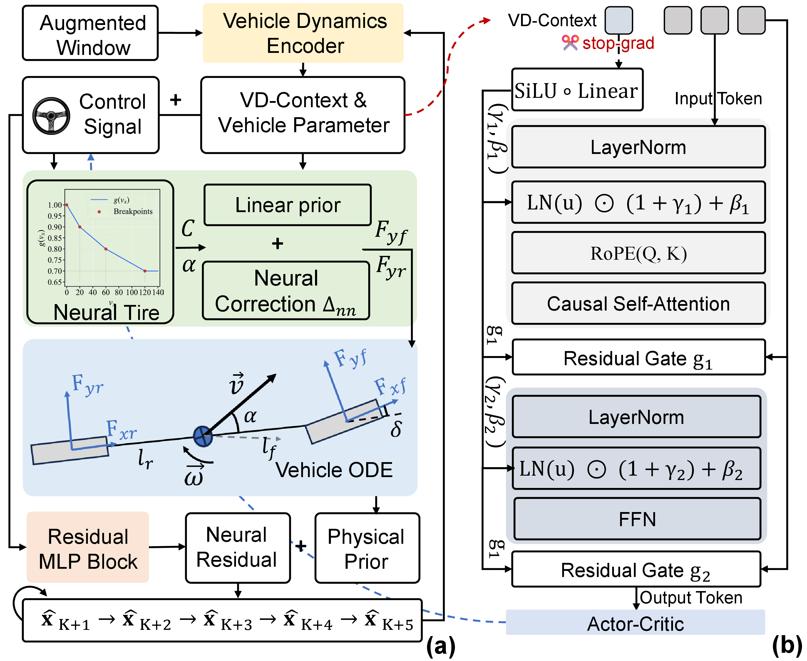
An ego-dynamics encoder-decoder is designed to extract and update a compact dynamics context \(\boldsymbol{\psi}_t\) from a sliding window of ego-vehicle states and actions. Let \(\mathbf{x}_t=[v_x,v_y,a_x,a_y,\omega,\dot{\omega}]^\top\) be the ego-vehicle states (longitudinal/lateral velocities, accelerations, yaw rate, and yaw acceleration), and \(\mathbf{a}_t=[a_{\mathrm{acc}},a_{\mathrm{steer}}]^\top\) be the corresponding normalized control inputs. Define the \(K\)-step context window \(\mathcal{W}_t=(\mathbf{x}_{t-K+1:t},\mathbf{a}_{t-K+1:t})\). The encoder-decoder comprises five sub-modules: \[\tag{3} \begin{alignat}{2} \text{Physics Aug.:}\quad & \boldsymbol{\Phi}_t &= {}& \phi_{\mathrm{phys}}(\mathcal{W}_t;{\boldsymbol{\theta}^{\mathrm{v}}}), \tag{4}\\ \text{VD-context Enc.:}\quad & (\boldsymbol{\psi}_t,\hat{\boldsymbol{\theta}^{\mathrm{v}}}_t) &= {}& \mathop{\mathrm{Enc}}_\xi(\mathcal{W}_t,\boldsymbol{\Phi}_t), \tag{5}\\ \text{Neural Tire:}\quad & F_y &= {}& \mathop{\mathrm{TireF}}(\alpha,v_x;C), \tag{6}\\ \text{Bicycle ODE:}\quad & \hat{\mathbf{x}}_{t+1}^{3} &= {}& \mathop{\mathrm{ODE}}(\mathbf{x}_t^{3},\mathbf{a}_t;\hat{\boldsymbol{\theta}^{\mathrm{v}}}_t), \tag{7}\\ \text{Dynamics Pred.:}\quad & \hat{\mathbf{x}}_{t+1} &= {}& \mathop{\mathrm{DynPred}}(\boldsymbol{\psi}_t,\mathbf{x}_t,\mathbf{a}_t;\hat{\boldsymbol{\theta}^{\mathrm{v}}}_t), \tag{8} \end{alignat}\] where \({\boldsymbol{\theta}^{\mathrm{v}}}\) is the chassis parameter vector, \(\boldsymbol{\Phi}_t\) is the physics-augmented feature vector at time \(t\), \(\alpha\) is the tire slip angle, \(C\) is the cornering stiffness coefficient, and \(\mathbf{x}_t^3=[v_x,v_y,\omega]^\top\) is the three-degree-of-freedom (3-DOF) lateral dynamics state. Fig. 2 (a) illustrates the complete encoder-decoder pipeline.
Build causal windows \(\mathcal{W}_t=(\mathbf{x}_{t-K+1:t},\mathbf{a}_{t-K+1:t})\) for \(t=1,\ldots,T\). Compute initial physics features \(\boldsymbol{\Phi}^{(1)}\) using \({\boldsymbol{\theta}^{\mathrm{v}}}_{\mathrm{nom}}\). \((\boldsymbol{\psi}_{1:T}^{(1)},\hat{\boldsymbol{\theta}^{\mathrm{v}}}_{1:T}^{(1)})\leftarrow\mathop{\mathrm{Enc}}_\xi(\mathcal{W}_{1:T},\boldsymbol{\Phi}^{(1)})\). Refine \(\boldsymbol{\Phi}^{(2)}\) using estimated \(\hat{\boldsymbol{\theta}^{\mathrm{v}}}_{1:T}^{(1)}\). \((\boldsymbol{\psi}_{1:T},\hat{\boldsymbol{\theta}^{\mathrm{v}}}_{1:T})\leftarrow\mathop{\mathrm{Enc}}_\xi(\mathcal{W}_{1:T},\boldsymbol{\Phi}^{(2)})\). Initialize \(\mathcal{L}_{\mathrm{aux}}\leftarrow 0\). Calculate \(\mathcal{L}_{\mathrm{aux}}\) and \(\mathcal{L}_{\mathrm{param}}\). \(\boldsymbol{\psi}_{1:T},\;\hat{\boldsymbol{\theta}^{\mathrm{v}}}_{1:T},\;\mathcal{L}_{\mathrm{aux}},\;\mathcal{L}_{\mathrm{param}}\).
4.1.2 Ego-dynamics encoder and parameter head↩︎
To augment inputs with physics information, six physics-informed features are derived from \(\mathcal{W}_t\): \[\phi_{\mathrm{phys}}\left(\mathcal{W}_t;{\boldsymbol{\theta}^{\mathrm{v}}}\right) = \bigl[\beta,\;v,\;\kappa,\;\tilde{F}_x,\;\tilde{F}_y,\;\tilde{M}_z\bigr], \label{eq:phys-feat}\tag{9}\] where \(\beta=\arctan(v_y/v_x)\) is the side-slip angle, \(v=\|(v_x,v_y)\|\) is the speed, \(\kappa=\omega/v\) is the trajectory curvature, and \((\tilde{F}_x,\tilde{F}_y,\tilde{M}_z)\) are coarse vehicle-level force and moment estimates derived from the identified mass and yaw inertia. A Gated Recurrent Unit (GRU) encodes the augmented sequence \([\mathbf{x}_{t-K+1:t};\boldsymbol{\Phi}_t;\mathbf{a}_{t-K+1:t}]\) into \(\boldsymbol{\psi}_t\).
The parameter vector \({\boldsymbol{\theta}^{\mathrm{v}}}=[m,\,I_z,\,l_f,\,l_r,\,C_f,\,C_r,\,\delta_{\max}]^\top\) collects the chassis quantities governing lateral vehicle dynamics: mass, yaw inertia, axle distances, cornering stiffnesses, and maximum steering angle. Computing \(\boldsymbol{\Phi}_t\) requires \({\boldsymbol{\theta}^{\mathrm{v}}}\), which is itself the identification target; encoding therefore proceeds in two weight-shared stages that bootstrap the physics features from nominal parameters \({\boldsymbol{\theta}^{\mathrm{v}}}_{\mathrm{nom}}\) and refine them with the first-stage estimate to yield the final \(\boldsymbol{\psi}_t\) and \(\hat{\boldsymbol{\theta}^{\mathrm{v}}}_t\). The parameter head maps \(\boldsymbol{\psi}_t\) to \(\hat{\boldsymbol{\theta}^{\mathrm{v}}}_t\) through a \(\tanh\)-bounded log-space multilayer perceptron (MLP), constraining \(\hat{\boldsymbol{\theta}^{\mathrm{v}}}_t\) to a physically plausible multiplicative offset from \({\boldsymbol{\theta}^{\mathrm{v}}}_{\mathrm{nom}}\).
4.1.3 Neural tire model↩︎
A tire model maps axle slip angles and cornering stiffnesses to lateral forces, forming the physical link between \(\hat{\boldsymbol{\theta}^{\mathrm{v}}}_t\) and the bicycle ODE. A linear tire model cannot capture the nonlinear saturation that dominates lateral force at high slip angles, yet a purely data-driven replacement discards the causal structure required for stable ODE integration. To reconcile fidelity with physical tractability, the lateral force is modeled as a linear prior plus a zero-initialized neural correction: \[\mathop{\mathrm{TireF}}\left(\alpha,v_x;C\right) \;=\; \underbrace{-C\alpha}_{\text{linear prior}} \;+\; \underbrace{\Delta_{\mathrm{nn}}\left(\alpha,v_x,C\right)}_{\text{neural correction}}, \label{eq:neural-tire}\tag{10}\] where \(\Delta_{\mathrm{nn}}\) is a two-hidden-layer MLP with \(\tanh\) activations. Zero initialization ensures that at the start of training \(\Delta_{\mathrm{nn}}\equiv 0\), reducing the dynamics to a linear bicycle model; the network then progressively captures saturation and speed-dependent stiffness. The per-axle stiffnesses \(C\in\{C_f,C_r\}\) and axle offsets \((l_f,l_r)\) are drawn from \(\hat{\boldsymbol{\theta}^{\mathrm{v}}}_t\); the front and rear slip angles derive from \(\mathbf{x}_t^3\): \[\alpha_f = \delta - \arctan\tfrac{v_y+l_f \omega}{v_x}, \qquad \alpha_r = -\arctan\tfrac{v_y-l_r \omega}{v_x}, \label{eq:slip-angles}\tag{11}\] where \(\delta=a_{\mathrm{steer}}\cdot g(v_x)\cdot\delta_{\max}\) is the estimated front-wheel steering angle, and \(g(v_x)\) is a fixed piecewise-linear speed-attenuation curve that accounts for the speed-dependent steering gain.
4.1.4 Bicycle model ODE↩︎
A single-track bicycle ODE combines the lateral forces from the tire model with the identified parameters \(\hat{\boldsymbol{\theta}^{\mathrm{v}}}_t\) to forward-predict the kinematic states. Let \(F_{yf}=\mathop{\mathrm{TireF}}(\alpha_f,v_x;C_f)\) and \(F_{yr}=\mathop{\mathrm{TireF}}(\alpha_r,v_x;C_r)\) denote the front and rear axle lateral forces given by Eq. 10 . Let \(F_{xr}=a_{\mathrm{acc}}\,m\,a_{\max}\) denote the rear longitudinal force, where \(a_{\max}\) is a fixed acceleration limit, and let \(\delta\) denote the front wheel angle defined below Eq. 11 . The evolution of \(\mathbf{x}_t^3\) is then governed by the single-track bicycle model [27]: \[\begin{align} \dot{v}_x &= \frac{F_{xr}-F_{yf}\sin\delta}{m}+v_y \omega,\\ \dot{v}_y &= \frac{F_{yf}\cos\delta+F_{yr}}{m}-v_x \omega,\\ \dot{\omega} &= \frac{l_f F_{yf}\cos\delta - l_r F_{yr}}{I_z}. \label{eq:bicycle-ode} \end{align}\tag{12}\]
The decoded parameter vector \(\hat{\boldsymbol{\theta}^{\mathrm{v}}}_t\) supplies all vehicle-specific quantities (\(m, I_z, l_f, l_r\)). Eq. 12 is integrated with a forward Euler step of size \(\Delta t\); the remaining three state components \((a_x,a_y,\dot{\omega})\) are recovered by finite differences.
The physics-informed ODE embeds causal structure to prevent physically implausible rollouts and improve data efficiency. Its explicit parameter interface further allows \(\hat{\boldsymbol{\theta}^{\mathrm{v}}}_t\) to be supervised by ground-truth chassis parameters, tying \(\boldsymbol{\psi}_t\) to identifiable physical quantities.
4.1.5 Dynamics predictor↩︎
The single-track bicycle ODE provides a physically grounded prior but cannot represent higher-order effects excluded by the single-track assumption. A neural residual conditioned on \(\boldsymbol{\psi}_t\) augments the physics prior to capture these unmodeled dynamics. \(\mathop{\mathrm{DynPred}}(\boldsymbol{\psi}_t,\mathbf{x}_t,\mathbf{a}_t;\hat{\boldsymbol{\theta}^{\mathrm{v}}}_t)\) composes the bicycle ODE step with a zero-initialized neural residual operating in normalized state space: \[\hat{\mathbf{x}}_{t+1} \;=\; \underbrace{\mathop{\mathrm{ODE}}\left(\mathbf{x}_t^{3},\mathbf{a}_t;\hat{\boldsymbol{\theta}^{\mathrm{v}}}_t\right)}_{\text{physics prior}} \;+\; \underbrace{\eta_\xi\left(\boldsymbol{\psi}_t,\mathbf{x}_t,\mathbf{a}_t\right)}_{\text{neural residual}}, \label{eq:dynpred}\tag{13}\] where \(\mathop{\mathrm{ODE}}(\cdot)\) denotes the Euler-discretized bicycle step, and \(\eta_\xi\) is a residual MLP block initialized to zero so that training starts from the pure physics prediction. The neural residual progressively absorbs suspension effects, load transfer, and other modeling errors that the single-track approximation cannot represent.
4.1.6 Auxiliary losses↩︎
The ego-dynamics neural-ODE encoder-decoder is trained with two independently weighted losses, multi-step prediction loss \(\mathcal{L}_{\mathrm{aux}}\) and parameter identification loss \(\mathcal{L}_{\mathrm{param}}\); stop-gradient on \(\boldsymbol{\psi}_t\) isolates their gradients within this module. \(\mathcal{L}_{\mathrm{aux}}\) is a uniformly weighted \(K_{\mathrm{pred}}\)-step rollout loss. Starting from the ground-truth state \(\mathbf{x}_t\), predictions unroll autoregressively with gradients severed between steps through the ODE chain: \[\mathcal{L}_{\mathrm{aux}} \;=\; \tfrac{1}{K_{\mathrm{pred}}}\sum_{k=1}^{K_{\mathrm{pred}}} b_{t+k}\,\|\hat{\mathbf{x}}_{t+k}-\mathbf{x}_{t+k}\|_1, \label{eq:aux-loss}\tag{14}\] where \(\hat{\mathbf{x}}_{t+k}\) is the \(k\)-step prediction and \(b_{t+k}\in\{0,1\}\) is a binary mask that zeroes out steps at or after a collision boundary. \(\mathcal{L}_{\mathrm{param}}\) is defined in log space: \[\mathcal{L}_{\mathrm{param}} \;=\; \left\|\,\log\tfrac{\hat{\boldsymbol{\theta}^{\mathrm{v}}}_t}{{\boldsymbol{\theta}^{\mathrm{v}}}_{\mathrm{nom}}} - \log\tfrac{{\boldsymbol{\theta}^{\mathrm{v}}}^{\star}}{{\boldsymbol{\theta}^{\mathrm{v}}}_{\mathrm{nom}}}\,\right\|_2^2, \label{eq:param-loss}\tag{15}\] where \({\boldsymbol{\theta}^{\mathrm{v}}}^{\star}\) is the ground-truth chassis parameter vector. \(\mathcal{L}_{\mathrm{aux}}\) and \(\mathcal{L}_{\mathrm{param}}\) force \(\boldsymbol{\psi}_t\) to carry actionable, physically grounded information. Algorithm [alg:vd-encdec] summarizes the complete pipeline of the ego-dynamics encoder-decoder, which delivers \(\boldsymbol{\psi}_t\) as a self-consistent, physics-grounded ego-dynamics prior ready to be injected into the WM.
4.2 Ego-Dynamics-Modulated World Model↩︎
To reshape both the prior and posterior latents at every step, \(\boldsymbol{\psi}_t\) is integrated into the Transformer WM. The Transformer WM of Section 3 uses homogeneous pre-norm blocks and absolute position embeddings, neither of which can adapt to the ego-dynamics heterogeneity across vehicles. Each Transformer block is therefore restructured to accept \(\boldsymbol{\psi}_t\) through AdaLN modulation, while RoPE decouples position information from the modulation channel, as depicted in Fig. 2 (b).
4.2.1 AdaLN modulation↩︎
Following the Diffusion Transformer (DiT) [28], every attention sub-block and feed-forward network (FFN) sub-block in the sequence model is replaced by an AdaLN layer whose affine parameters and residual gate are produced from \(\boldsymbol{\psi}_t\): \[\begin{align} \tilde{\mathbf{u}} &= \mathop{\mathrm{LN}}\left(\mathbf{u}\right)\odot\left(1+\boldsymbol{\gamma}\left(\boldsymbol{\psi}_t\right)\right)+\mathbf{b}\left(\boldsymbol{\psi}_t\right),\\ \mathbf{u} &\leftarrow \mathbf{u} + \mathbf{g}\left(\boldsymbol{\psi}_t\right)\odot\mathop{\mathrm{Block}}\left(\tilde{\mathbf{u}}\right), \end{align} \label{eq:adaln}\tag{16}\] where \(\mathbf{u}\) is the input activation of the sub-block, \(\mathop{\mathrm{LN}}(\cdot)\) denotes Layer Normalization, \(\mathop{\mathrm{Block}}(\cdot)\) is the attention or FFN operation, and \((\boldsymbol{\gamma},\mathbf{b},\mathbf{g})\) are the scale, shift, and gate projections for the sub-block. Modulation weights are zero-initialized so that the block collapses to an affine identity before training, while gate biases are offset by \(0.5\) to keep the sub-block contribution non-zero from step zero. Any position encoding that carries ego-dynamics information would corrupt the modulation channel. Position encoding must therefore remain strictly orthogonal to \(\boldsymbol{\psi}_t\).
4.2.2 Position embedding↩︎
Absolute position embeddings are replaced with RoPE [29], a relative-position scheme that applies per-head rotations to query and key vectors as a function of token position alone. The critical design property is orthogonality: the rotation angle depends solely on token position and carries no information about \(\boldsymbol{\psi}_t\), so position encoding and AdaLN modulation operate on strictly disjoint channels. The KV cache therefore remains safely reusable as \(\boldsymbol{\psi}_t\) evolves across imagination steps.
4.2.3 Training objective and detached context↩︎
The WM loss inherits the composition of Eq. 1 ; the full DynaDreamer training objective is: \[\mathcal{L}^{\mathrm{DD}} = \mathcal{L}_{\mathrm{WM}}\left(\boldsymbol{\psi}_t\leftarrow\mathop{\mathrm{sg}}\left(\boldsymbol{\psi}_t\right)\right) + \alpha_{\mathrm{aux}}\mathcal{L}_{\mathrm{aux}} + \alpha_{\mathrm{param}}\mathcal{L}_{\mathrm{param}}, \label{eq:dd-loss}\tag{17}\] where \(\mathop{\mathrm{sg}}(\cdot)\) blocks gradient flow into the VD-context encoder, and \(\alpha_{\mathrm{aux}},\alpha_{\mathrm{param}}>0\) are scalar loss-weighting coefficients for the dynamics prediction and parameter-identification terms.
The VD-context \(\boldsymbol{\psi}_t\) is passed through a stop-gradient before entering the Transformer. This isolation prevents the WM from back-propagating reconstruction and KL gradients into the encoder \(\xi\), which would collapse \(\boldsymbol{\psi}_t\) onto dynamics-irrelevant pixel statistics. The encoder is thus trained exclusively by \(\mathcal{L}_{\mathrm{aux}}\) and \(\mathcal{L}_{\mathrm{param}}\), preserving the physics grounding of Section 4.1. \(\boldsymbol{\psi}_t\) is updated at every time step on a sliding window rather than held constant, which aligns WM learning and rollout.
4.3 Ego-Dynamics-Aligned Imagination Rollout↩︎
During training, \(\boldsymbol{\psi}_t\) is computed from the ground-truth ego-state window \(\mathcal{W}_t\) at every step. Imagination introduces three problems absent from training. First, future states are produced by the model rather than observed, so \(\boldsymbol{\psi}_t\) must be propagated by the physics predictor. Second, KV cache entries written at prior steps carry no dynamics imprint unless explicitly modulated before storage, leading to inconsistency with the current-step conditioning. Third, trajectories terminate at different steps in batched imagination, and continuing to update \(\boldsymbol{\psi}_t\) for terminated samples risks corrupting surviving ones. Three mechanisms address each problem in turn.
4.3.1 Modulated KV cache for autoregressive rollout↩︎
At every imagined step, the raw key \(\mathbf{k}_t\) and value \(\mathbf{v}_t\) produced by the Transformer are passed through pre-modulation \(\mathop{\mathrm{PreMod}}(\cdot\,;\boldsymbol{\psi}_t)\) to yield the modulated pair \((\tilde{\mathbf{k}}_t,\tilde{\mathbf{v}}_t)\), which is then written into the cache. Entries already in the cache remain untouched, so each token carries a permanent imprint of the ego-dynamics state under which it was produced while maintaining \(\mathcal{O}(H)\) autoregressive complexity.
4.3.2 Online VD-context update via ODE rollout↩︎
At the start of a rollout, the true chassis parameters are unavailable, so \(\boldsymbol{\psi}_{K_{\mathrm{ctx}}}\) at the rollout-start index \(K_{\mathrm{ctx}}\) is seeded with nominal parameters \({\boldsymbol{\theta}^{\mathrm{v}}}_{\mathrm{nom}}\), where \(K_{\mathrm{ctx}}\) denotes the warm-up context length distinct from the VD-context window size \(K\). From step \(K_{\mathrm{ctx}}\) onward, the identified parameters \(\hat{\boldsymbol{\theta}^{\mathrm{v}}}_t\) produced by the encoder replace the nominal prior, and the ego state is propagated by the physics-informed predictor: \[\begin{align} \hat{\mathbf{x}}_{t+1} &= \mathop{\mathrm{DynPred}}\left(\boldsymbol{\psi}_t,\hat{\mathbf{x}}_t,\mathbf{a}_t;\hat{\boldsymbol{\theta}^{\mathrm{v}}}_t\right),\\ \boldsymbol{\psi}_{t+1} &= \mathop{\mathrm{Enc}}_\xi\left(\mathcal{W}_{t+1},\,\phi_{\mathrm{phys}}\left(\mathcal{W}_{t+1};\hat{\boldsymbol{\theta}^{\mathrm{v}}}_t\right)\right), \label{eq:online-ctx} \end{align}\tag{18}\] where \(\mathcal{W}_{t+1}=(\hat{\mathbf{x}}_{t-K+2:t+1},\,\mathbf{a}_{t-K+2:t+1})\) slides forward by replacing real states with imagined ones while retaining the executed actions.
At deployment, a vehicle with different chassis dynamics produces a distinct ego-state window \(\mathcal{W}\) that shifts \(\boldsymbol{\psi}_t\) through the encoder and thereby steers the AdaLN modulation in Eq. 16 . The Transformer weights \(\phi\) require no retraining to adapt to the new dynamic characteristics.
4.3.3 Per-sample termination freezing↩︎
In batched imagination, samples terminate at different steps. A per-sample binary alive mask \(\nu_t\in\{0,1\}\) tracks whether each trajectory is still active. When a sample terminates (\(\nu_t=0\)), its \(\boldsymbol{\psi}_t\) is held at the last active value rather than updated, whereas live samples (\(\nu_t=1\)) continue to receive the refreshed context from the ODE predictor. This selective freezing prevents post-termination states from corrupting the WM forward pass of surviving samples. The actor only takes the WM latent \((\mathbf{h}_t,\mathbf{z}_t)\), keeping the policy gradient path independent of the encoder \(\xi\).
Algorithm [alg:dd-combined] summarizes training and imagination. Together, these three subsections close a loop between physics and pixels. The encoder-decoder extracts physics state into \(\boldsymbol{\psi}_t\) and \(\hat{\boldsymbol{\theta}^{\mathrm{v}}}_t\); the AdaLN-RoPE Transformer lets \(\boldsymbol{\psi}_t\) reshape the latent distribution while keeping encoder gradients isolated; and the modulated imagination procedure keeps \(\boldsymbol{\psi}_t\) synchronized with the ODE predictor during rollout. The actor is thereby optimized in a WM whose imagined responses are aligned with physics-driven ego-dynamics.
Sample a batch \((\mathbf{o}_{1:T},\mathbf{a}_{1:T},r_{1:T},n_{1:T},\mathbf{x}_{1:T},{\boldsymbol{\theta}^{\mathrm{v}}}^{\star})\sim\mathcal{D}\). \((\boldsymbol{\psi}_{1:T},\hat{\boldsymbol{\theta}^{\mathrm{v}}}_{1:T},\mathcal{L}_{\mathrm{aux}},\mathcal{L}_{\mathrm{param}})\leftarrow\boldsymbol{Algorithm~\ref{alg:vd-encdec}}\). \(\boldsymbol{\psi}'_{1:T}\leftarrow \mathop{\mathrm{sg}}(\boldsymbol{\psi}_{1:T})\). Encode observations: \(\mathbf{e}_{1:T}=\mathop{\mathrm{Embed}}(\mathbf{z}_{1:T},\mathbf{a}_{1:T})\). \(\mathbf{h}_{1:T}\leftarrow f_\phi\bigl(\mathbf{e}_{1:T};\;\mathop{\mathrm{RoPE}},\;\mathop{\mathrm{AdaLN}}(\boldsymbol{\psi}'_{1:T})\bigr)\). Decode reconstruction, reward, and continuation heads. Compute \(\mathcal{L}_{\mathrm{WM}}\) from Eq. 1 . \(\mathcal{L}^{\mathrm{DD}}\leftarrow \mathcal{L}_{\mathrm{WM}} + \alpha_{\mathrm{aux}}\mathcal{L}_{\mathrm{aux}}+\alpha_{\mathrm{param}}\mathcal{L}_{\mathrm{param}}\). Update \(\phi\) via \(\nabla_\phi\mathcal{L}_{\mathrm{WM}}\) and \(\xi\) via \(\nabla_\xi\left(\mathcal{L}_{\mathrm{aux}}+\mathcal{L}_{\mathrm{param}}\right)\). Reset KV cache; encode warm-up context to obtain \(\mathbf{h}_{K_{\mathrm{ctx}}},\mathbf{z}_{K_{\mathrm{ctx}}}\). Initialize \(\boldsymbol{\psi}_{K_{\mathrm{ctx}}}\leftarrow\mathop{\mathrm{Enc}}_\xi(\mathcal{W}_{K_{\mathrm{ctx}}},\phi_{\mathrm{phys}}(\mathcal{W}_{K_{\mathrm{ctx}}};{\boldsymbol{\theta}^{\mathrm{v}}}_{\mathrm{nom}}))\);\(\hat{\mathbf{x}}_{K_{\mathrm{ctx}}}\leftarrow\mathbf{x}_{K_{\mathrm{ctx}}}\);\(\nu_{K_{\mathrm{ctx}}}\leftarrow 1\). Form imagined trajectory \(\tau=(\mathbf{h},\mathbf{z},\mathbf{a},\hat{r},\hat{n})_{K_{\mathrm{ctx}}:K_{\mathrm{ctx}}+H}\) and \(\lambda\)-return of Eq. 2 . Update \(\pi_\theta,V_\rho\) on \(\tau\).
5 Theoretical Insights into the Ego-Dynamics Prior↩︎
This section provides an information-theoretic analysis of why augmenting the world model with an ego-dynamics prior eases learning. The analysis adopts the following assumptions: (i) Lipschitz vehicle dynamics, (ii) additive observation noise, (iii) a \(\beta\)-mixing observation–action process [30], (iv) an exploratory policy that renders dynamically distinct chassis distinguishable, and (v) conditional independence of the object-induced flow \(\Delta_t\) (defined in Eq. 19 ) from the ego-dynamics context given the current observation and action. The chassis context \(c\), instantiated by the physical parameter vector \({\boldsymbol{\theta}^{\mathrm{v}}}\) of Section 4.1, depends only on the vehicle. \(H(\cdot)\) and \(I(\cdot\,;\cdot)\) denote the (differential) entropy and mutual information, respectively [31]. The results are stated as propositions with proofs that emphasize the key reasoning steps.
5.1 Egocentric Observation Model↩︎
Let \(\xi_t\in SE(2)\) be the ego-vehicle pose, and let \(g_t\triangleq\xi_t^{-1}\xi_{t+1}\) denote the one-step relative ego motion expressed in the current ego frame. The vehicle dynamics determine \(g_t\) as \(g_t=G(\mathbf{x}_t,\mathbf{a}_t;c)\). The BEV is rendered around the ego vehicle, so the static background transforms rigidly with the viewpoint change. Consecutive observations therefore obey the following decomposition: \[\mathbf{o}_{t+1}=\mathcal{W}_{g_t}(\mathbf{o}_t)\;\oplus\;\Delta_t, \label{eq:flow-decomp}\tag{19}\] where \(\mathcal{W}_{g_t}(\mathbf{o}_t)\) is the ego-induced flow, i.e.the rigid image warp of \(\mathbf{o}_t\) under the ego motion \(g_t\); \(\oplus\) denotes pixel-wise composition; and \(\Delta_t\) is the object-induced flow, collecting the genuine motion of surrounding agents together with content entering or leaving the field of view. This decomposition mirrors the classical separation of an observed flow field into camera-motion and object-motion components [32]. The first term is fixed once \(g_t\) is known; only the second reflects what the WM must genuinely predict.
5.2 The Ego-Motion Modeling Burden↩︎
Proposition 1 (Ego-motion modeling burden). Under the egocentric model of Eq. 19 , the conditional entropy of the next observation is decomposed as: \[H(\mathbf{o}_{t+1}\mid\mathbf{o}_t,\mathbf{a}_t)=I(g_t;\mathbf{o}_{t+1}\mid\mathbf{o}_t,\mathbf{a}_t)+H(\mathbf{o}_{t+1}\mid\mathbf{o}_t,\mathbf{a}_t,g_t), \label{eq:entropy-decomp}\qquad{(1)}\] where the first term is the ego-motion burden, i.e.the predictive uncertainty that arises solely from not knowing \(g_t\). Conditioning on any statistic that determines \(g_t\) removes at least this quantity from the predictive entropy, with equality for a statistic informationally equivalent to \(g_t\).
Proof. The decomposition is a direct application of the chain rule of conditional entropy. The warp \(\mathcal{W}_{g_t}\) is deterministic given \(g_t\), so the mutual information term is precisely the burden a pixel-only model spends on ego-motion. The entropy reduction under additional conditioning holds by the data processing inequality. \(\square\)
Proposition 2 (Geometric amplification and chassis multimodality). The ego-motion burden is (i) geometrically amplified, as the warp displaces content at scene radius \(\rho\) by \(\approx\rho\,|\Delta\theta_t|\) for an ego rotation \(\Delta\theta_t\), and (ii) chassis-dependent: \[H(\mathbf{o}_{t+1}\!\mid\!\mathbf{o}_t,\mathbf{a}_t)=H(\mathbf{o}_{t+1}\!\mid\!\mathbf{o}_t,\mathbf{a}_t,c)+I(c;\mathbf{o}_{t+1}\!\mid\!\mathbf{o}_t,\mathbf{a}_t), \label{eq:chassis-decomp}\qquad{(2)}\] where the equality is the conditional mutual information identity applied to \(c\). The non-trivial claim is \(I(c;\mathbf{o}_{t+1}\mid\mathbf{o}_t,\mathbf{a}_t)>0\) whenever dynamically distinct chassis are excited.
Proof. The equality follows from the chain rule of conditional entropy. The strictly positive mutual information holds under assumptions (i) and (iv): distinct chassis produce distinct ego-motions \(g_t\) under the same action, which in turn induce distinct observation warps. A pixel-only WM must therefore identify \(c\) implicitly to remain Markov in \((\mathbf{o}_t,\mathbf{a}_t)\). \(\square\)
5.3 The Prior–Posterior Bottleneck and Its Resolution↩︎
The Transformer WM exposes the full history through its KV cache, and the bottleneck therefore lies not in model capacity but in the information asymmetry between prior and posterior. The posterior has access to \(\mathbf{o}_{t+1}\) and can therefore recover the realized ego-motion \(g_t\) via Eq. 19 . The observation-free prior, by contrast, must predict \(g_t\) from history alone, creating an irreducible misalignment whenever \(g_t\) varies across chassis.
Proposition 3 (Prior–posterior bottleneck). For the latent WM with an optimal observation-free prior, the minimal expected dynamics KL at step \(t{+}1\) satisfies: \[\begin{align} \min_{p}\;\mathbb{E}&\big[\mathop{\mathrm{KL}}\!\left(q_\phi(\mathbf{z}_{t+1}\mid\mathbf{h}_{t+1},\mathbf{o}_{t+1})\,\|\,p(\mathbf{z}_{t+1}\mid\mathbf{h}_{t+1})\right)\big]\\ &=I(\mathbf{z}_{t+1};\mathbf{o}_{t+1}\mid\mathbf{h}_{t+1})\;\ge\;I(\mathbf{z}_{t+1};g_t\mid\mathbf{h}_{t+1}). \end{align} \label{eq:kl-bound}\qquad{(3)}\] Under chassis randomization, \(\mathbf{h}_{t+1}\) does not determine \(g_t\), so \(I(\mathbf{z}_{t+1};g_t\mid\mathbf{h}_{t+1})>0\) is an irreducible prior–posterior misalignment. Conditioning the prior on \(\boldsymbol{\psi}_t\) (the VD-context of Section 4.1) lowers the achievable bound to \(I(\mathbf{z}_{t+1};\mathbf{o}_{t+1}\mid\mathbf{h}_{t+1},\boldsymbol{\psi}_t)\), removing exactly the ego-motion misalignment: \[\begin{align} \Delta_{\mathop{\mathrm{KL}}}&=I(\mathbf{z}_{t+1};\mathbf{o}_{t+1}\mid\mathbf{h}_{t+1})-I(\mathbf{z}_{t+1};\mathbf{o}_{t+1}\mid\mathbf{h}_{t+1},\boldsymbol{\psi}_t)\\ &=I(\mathbf{z}_{t+1};g_t\mid\mathbf{h}_{t+1})>0. \end{align} \label{eq:delta-kl}\qquad{(4)}\]
Proof. The optimal observation-free prior is the aggregated posterior \(p^\star(\mathbf{z}_{t+1}\mid\mathbf{h}_{t+1})=\mathbb{E}_{\mathbf{o}_{t+1}}[q_\phi(\mathbf{z}_{t+1}\mid\mathbf{h}_{t+1},\mathbf{o}_{t+1})]\), for which the average KL equals \(I(\mathbf{z}_{t+1};\mathbf{o}_{t+1}\mid\mathbf{h}_{t+1})\) [33]. Reconstruction-sufficiency with Eq. 19 gives the lower bound, as \(g_t\) is recoverable from \((\mathbf{o}_t,\mathbf{o}_{t+1})\) and \(\mathbf{o}_t\) is summarized in \(\mathbf{h}_{t+1}\). For the KL reduction, the chain rule gives \(\Delta_{\mathop{\mathrm{KL}}}=I(\mathbf{z}_{t+1};\boldsymbol{\psi}_t\mid\mathbf{h}_{t+1})-I(\mathbf{z}_{t+1};\boldsymbol{\psi}_t\mid\mathbf{h}_{t+1},\mathbf{o}_{t+1})\). The second term vanishes: once \(\mathbf{o}_{t+1}\) is observed, \(g_t\) is determined, and \(\boldsymbol{\psi}_t\) provides no further information about \(\mathbf{z}_{t+1}\) given sufficiency (Proposition 4). The first term reduces to \(I(\mathbf{z}_{t+1};g_t\mid\mathbf{h}_{t+1})\) by assumption (v), which ensures that \(\boldsymbol{\psi}_t\) informs \(\mathbf{z}_{t+1}\) only through \(g_t\). \(\square\)
Proposition 4 (Sufficiency of the ego-dynamics prior). Under universal approximation of the encoder \(\mathop{\mathrm{Enc}}_\xi\) and predictor \(\mathop{\mathrm{DynPred}}\), and a \(\beta\)-mixing excitation window of length \(K\) that renders the chassis identifiable from the state–action history, the physics-informed predictor of Section 4.1, trained to minimize \(\mathcal{L}_{\mathrm{aux}}\) and \(\mathcal{L}_{\mathrm{param}}\), makes \(\boldsymbol{\psi}_t\) sufficient for \(g_t\) in the limit of vanishing training loss, i.e.\(I(g_t;\mathbf{o}_{t+1}\mid\mathbf{o}_t,\mathbf{a}_t,\boldsymbol{\psi}_t)\to 0\) as \(\mathcal{L}_{\mathrm{aux}}\to 0\). The reductions in Propositions 1 and 3 are therefore attained.
Proof. Under \(\beta\)-mixing, a window of \(K\) consecutive state–action pairs \(\mathcal{W}_t\) carries sufficient information to identify the chassis context \(c\) up to the intrinsic ambiguity of the dynamics [30]. The universal-approximation capacity of \(\mathop{\mathrm{Enc}}_\xi\) ensures that the mapping from \(\mathcal{W}_t\) to \((\boldsymbol{\psi}_t,\hat{\boldsymbol{\theta}^{\mathrm{v}}}_t)\) can represent the required inverse identification map. When \(\mathcal{L}_{\mathrm{aux}}\to 0\), the predictor \(\mathop{\mathrm{DynPred}}\) recovers the true next state \(\mathbf{x}_{t+1}\) from \((\boldsymbol{\psi}_t,\mathbf{x}_t,\mathbf{a}_t)\), which determines \(g_t=G(\mathbf{x}_t,\mathbf{a}_t;c)\). Hence \(g_t\) becomes a deterministic function of \(\boldsymbol{\psi}_t\) and the current state–action pair, yielding \(I(g_t;\mathbf{o}_{t+1}\mid\mathbf{o}_t,\mathbf{a}_t,\boldsymbol{\psi}_t)\to 0\). \(\square\)
Corollary 1 (Bounded imagination drift). During imagination only the prior is rolled out (Section 3). Without an ego-dynamics prior, the unpredictable ego-motion error compounds over the horizon \(H\). Refreshing \(\boldsymbol{\psi}_t\) through the online ODE predictor of Section 4.3 makes \(g_t\) predictable from the prior at each step. Each step’s ego-motion prediction error then reduces to the ODE predictor error \(\epsilon_{\mathrm{ode}}\), and the cumulative drift over horizon \(H\) is bounded by \(\mathcal{O}(H\,\epsilon_{\mathrm{ode}})\).
Corollary 2 (Zero-shot cross-chassis transfer). The ego-dynamics prior \(\boldsymbol{\psi}_t\) is parameterized through the identifiable chassis parameters \(\hat{\boldsymbol{\theta}^{\mathrm{v}}}_t\) rather than memorized appearance. Under the identifiability assumption, an unseen chassis \(c'\) yields a re-identified \(\hat{\boldsymbol{\theta}^{\mathrm{v}}}_t\) that relocates the prior to the new dynamics regime, enabling the WM and policy to adapt without retraining.
In summary, the bottleneck is one of representation rather than capacity. Ego-motion is determined by the executed action and the chassis, yet the observation-free prior cannot anticipate it. This unpredictability inflates the prior–posterior KL (Proposition 3). Unlike a generic learned context, the ego-dynamics prior is a physically identifiable sufficient statistic paired with a physics-informed ODE predictor. These two properties are precisely what enable prior-only imagination (Corollary 1) and zero-shot transfer (Corollary 2).
6 Experiments↩︎
6.1 Experimental Setup↩︎
The simulation environment is based on CarDreamer [34], a platform for WM-based autonomous driving built atop the CARLA simulator [35]. To highlight diverse driving skill learning, we improve CarDreamer by configuring random tasks in Town03 (Urban) and Town04 (Highway) as shown in Fig. 3. Each scenario features background traffic flow governed by the IDM and MOBIL models. The simulation runs at a fixed frequency of 10 Hz. The agent uses a continuous action configuration \(\mathbf{a}=[a_{\mathrm{acc}},\,a_{\mathrm{steer}}]^\top\) with \(a_{\mathrm{acc}}, a_{\mathrm{steer}}\in[-1,1]\). An episode terminates upon collision, timeout (500 steps), out-of-lane violation, or destination arrival.

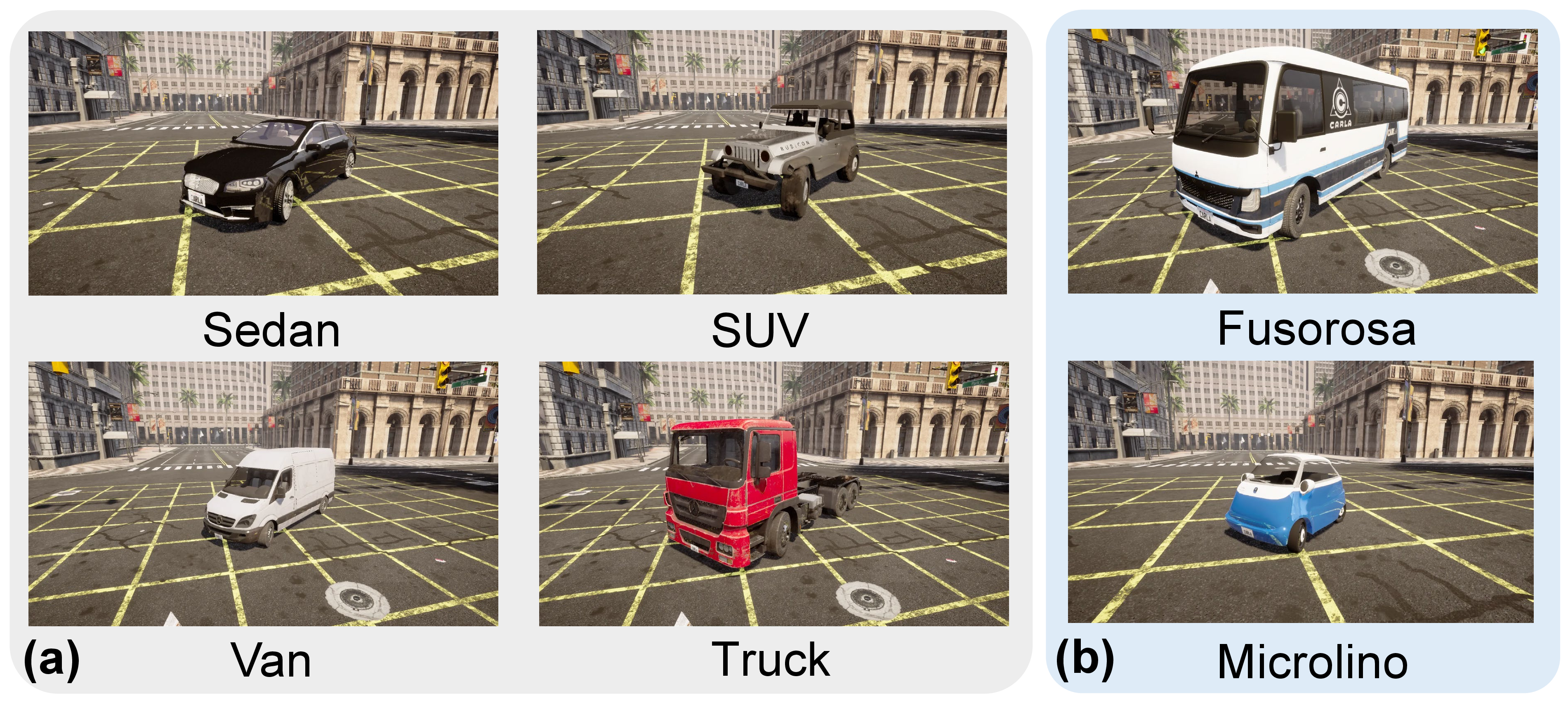
To evaluate generalization across diverse chassis dynamics and test whether the agent captures underlying physical principles, domain randomization in vehicle dynamics during training is applied. As shown in Table ¿tbl:tab:vehicle95chassis95categories?, the training set comprises 17 vehicle variants spanning four chassis categories (sedan, SUV, van, truck) with distinct control characteristics, while two additional vehicles are reserved for zero-shot evaluation (Fig. 4). This randomization instantiates the chassis-conditioned multimodality of Proposition 2: under an identical policy, dynamically distinct chassis drive the same scene to different temporal evolutions, which the world model must disentangle. To yield a wide distribution of chassis-dynamics features, nine PhysX tire-model parameters are randomized per vehicle instance: multiplicative scale factors drawn from \([0.7,\,1.5]\) are applied to mass, drag coefficient, tire friction, damping rate, maximum steering angle, and lateral and longitudinal stiffness; the center-of-mass (CoM) \(x\)-offsets and \(z\)-offsets receive additive perturbations drawn uniformly from \([-0.15,\,0.15]\) m and \([-0.05,\,0.05]\) m, respectively. For each vehicle, we extract the ground-truth parameter vector \({\boldsymbol{\theta}^{\mathrm{v}}}^\star\) from the PhysX tire model.
@c>p0.9cmc>p1.2cmc>p5.9cmc@ & Category & Variant ID
& Sedan & Coupe, MKZ, Mustang, TT, Model3
& SUV & Patrol_21, Patrol, Wrangler, e-tron
& Van & Ambulance, Sprinter, T2, T2_21
& Truck & Euro_HGV, Firetruck, Cybertruck, CarlaCola
& Bus & Fusorosa
& Micro & Microlino
The primary observation is a BEV image of size \(128\times128\times3\), containing four semantic layers: road map, planned waypoints, ego vehicle, and surrounding traffic vehicles as shown in Fig. 3. The composite reward at timestep \(t\) is: \[\begin{align} r_t &= r_{\mathrm{spd}} + r_{\mathrm{lat}} + r_{\mathrm{hdg}} + r_{\mathrm{wpt}} + r_{\mathrm{stb}} + r_{\mathrm{col}} + r_{\mathrm{dst}}, \nonumber \\ r_{\mathrm{spd}} &= w_v\varphi - w_v\max\left(0,\tfrac{v_\parallel - v_{\mathrm{des}}}{v_{\mathrm{des}}}\right) - \tfrac{1}{2}\min\left(v_\perp,\,1\right), \nonumber \\ r_{\mathrm{lat}} &= w_d\,\varphi\,\exp\left(-d_\perp^2/\sigma^2\right), \nonumber \\ r_{\mathrm{hdg}} &= w_\theta\bigl[\varphi\max\left(\cos\Delta\theta,\,0\right) + \min\left(\cos\Delta\theta,\,0\right)\bigr], \nonumber \\ r_{\mathrm{wpt}} &= w_{\mathrm{wpt}}\,\mathbf{1}[\Delta n_{\mathrm{wpt}}>0], \label{eq:reward} \\ r_{\mathrm{stb}} &= -w_s\bigl[\max\left(|a_y|-1.5,\,0\right) + 0.05\max\left(|\dot{\omega}|-8,\,0\right)\bigr], \nonumber \\ r_{\mathrm{col}} &= -w_c\max\left(v,\,1\right)\,\mathbf{1}[\text{collision}], \nonumber \\ r_{\mathrm{dst}} &= w_{\mathrm{dst}}\,\mathbf{1}[\text{goal reached}]. \nonumber \end{align}\tag{20}\] where \(\varphi = \mathrm{clip}(v_\parallel/v_{\mathrm{des}},\,0,\,1)\) is the speed-gating factor, with \(v_\parallel\) the path-tangential ego speed, \(v_\perp\) the lateral ego speed, and \(v_{\mathrm{des}}\) the target speed; \(d_\perp\) is the cross-track deviation; \(\Delta\theta\) the heading error; \(\Delta n_{\mathrm{wpt}}\) the number of waypoints completed in the step; \(a_y\) the lateral acceleration; and \(\dot{\omega}\) the yaw acceleration. Weights: \(w_v{=}2.0\), \(w_d{=}1.0\), \(w_\theta{=}0.5\), \(w_{\mathrm{wpt}}{=}2.0\), \(w_s{=}0.02\), \(w_c{=}30\), \(w_{\mathrm{dst}}{=}20\); \(\sigma{=}1.5\) m. The speed gate \(\varphi\) ensures a stationary vehicle receives zero dense reward, preventing exploitation without forward motion; the dead zone in \(r_{\mathrm{stb}}\) (\(|a_y|<1.5\) m/s\(^2\), \(|\dot{\omega}|<8\) rad/s\(^2\)) permits normal cornering without penalty.
6.2 Training Details↩︎
We implement DynaDreamer on STORM [26], and compare DynaDreamer against baselines and ablation variants.
6.2.1 Baselines↩︎
(1) SAC (Soft Actor-Critic) [36]: a model-free RL method with a convolutional neural network (CNN) encoder. (2) DreamerV3 [10]: a model-based method using a recurrent state-space model (RSSM) as its WM. (3) STORM [26]: a Transformer-based WM, and an actor-critic agent trained from imagined rollouts. (4) VD-STORM: STORM equipped with the same VD-context and ego-dynamics modules as DynaDreamer, but \(\boldsymbol{\psi}_t\) only enters the actor-critic, with the WM left unchanged.
6.2.2 Ablation variants↩︎
(1) w/o Neural-ODE: replaces the physics-informed dynamics predictor (bicycle ODE, neural tire model, and neural residual) with a pure residual MLP; the parameter estimation head and physics-informed features are removed. (2) w/o Modulation: replaces AdaLN conditioning with concatenation of \(\boldsymbol{\psi}_t\) at the Transformer input stem; RoPE is replaced by absolute positional encoding. (3) w/o Multi-step: sets the auxiliary prediction horizon to \(K_{\mathrm{pred}}{=}1\) (single-step) instead of \(K_{\mathrm{pred}}{=}5\) (autoregressive multi-step).
6.2.3 Evaluation protocol↩︎
Each method is evaluated over 300 episodes partitioned into three conditions. S1 (in-distribution, 100 episodes): vehicles are randomly drawn from the 17 vehicle variant training pool, probing performance under familiar dynamics. S2 (zero-shot, 100 episodes): the unseen Fusorosa, a large bus-class vehicle with substantially heavier mass and longer wheelbase than any training variant. S3 (zero-shot, 100 episodes): the unseen Microlino, a micro-class vehicle with an unusually short wheelbase and low mass. S2 and S3 together probe whether the ego-dynamics prior generalizes to handling regimes outside the training distribution. We report 5 categories of metrics:
Task completion: success rate, collision rate, out-of-lane rate, timeout rate, cumulative reward.
Driving quality: heading error, lateral deviation, average jerk, average speed.
BEV reconstruction: peak signal-to-noise ratio (PSNR), mean absolute error (MAE).
Low-dimensional state prediction: MAE at different horizons (\(H{=}1,3,5\)) and per-component breakdown.
Chassis parameter estimation: relative error mean \(\bigl(\frac{1}{7}\sum_{k=1}^{7}|[\hat{{\boldsymbol{\theta}^{\mathrm{v}}}}]_k - [{\boldsymbol{\theta}^{\mathrm{v}}}^\star]_k|/|[{\boldsymbol{\theta}^{\mathrm{v}}}^\star]_k|\bigr)\), log-space mean squared error (MSE) \(\bigl(\frac{1}{7}\sum_{k=1}^{7}(\log[\hat{{\boldsymbol{\theta}^{\mathrm{v}}}}]_k - \log[{\boldsymbol{\theta}^{\mathrm{v}}}^\star]_k)^2\bigr)\), and consistency (standard deviation of relative errors across episodes).
6.2.4 Implementation details↩︎
Table 1 summarizes the training hyperparameters. All STORM-based methods share the same backbone architecture. On Town03, all methods are trained for \(10^5\) real-interaction steps; on Town04, \(5\times10^4\) steps suffice as the simpler highway geometry leads to faster convergence. All methods use a replay buffer of \(10^5\) transitions and a warm-up of 1024 random steps. Three random seeds are used for reproduction.
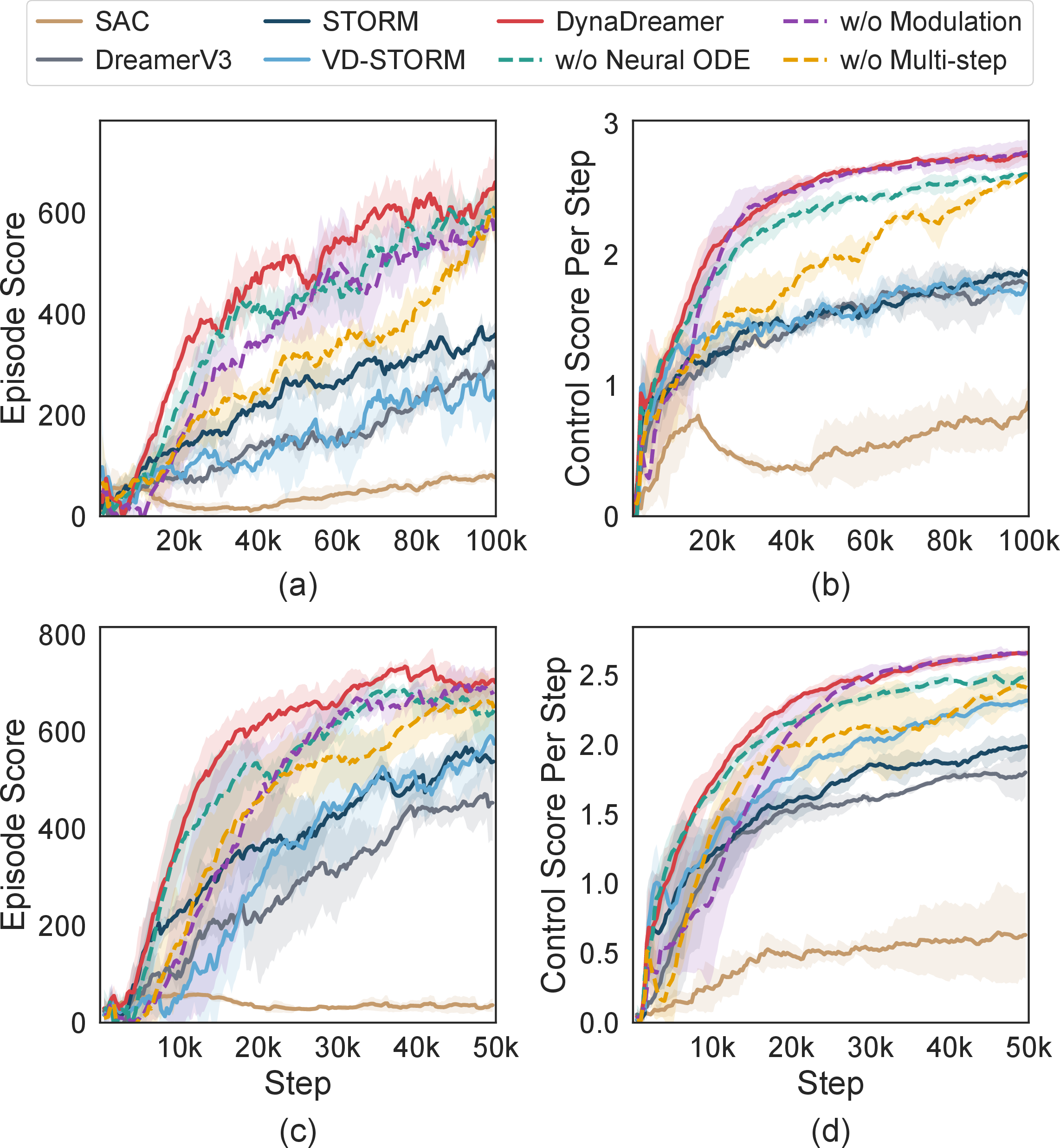
Fig. 5 presents the training curves on Town03 (Fig. 5 (a)-(b)) and Town04 (Fig. 5 (c)-(d)). SAC fails to converge on both Town03 and Town04 and is excluded from subsequent evaluation. On Town03, DynaDreamer converges to the highest episode score and control score across all remaining baselines and ablation variants, demonstrating stable and efficient learning throughout training. On Town04, DynaDreamer again attains the highest episode score and control score across all compared methods.
| Hyperparameter | Description | Value | ||||
|---|---|---|---|---|---|---|
| \(\mathrm{lr}_{\mathrm{wm}}\) | WM learning rate | \(1{\times}10^{-4}\) | ||||
| \(\mathrm{lr}_{\mathrm{agent}}\) | Agent learning rate | \(3{\times}10^{-5}\) | ||||
| \(B \times T\) | Batch size (seq.\(\times\) length) | \(16 \times 64\) | ||||
| \(|\mathcal{D}|\) | Replay buffer capacity | \(10^{5}\) | ||||
| \(\gamma\) | Discount factor | 0.99 | ||||
| \(\lambda\) | Trace-decay coefficient | 0.95 | ||||
| \(H\) | Imagination horizon | 16 | ||||
| \(K_{\mathrm{ctx}}\) | Imag.warm-up context | 8 | ||||
| \(\beta_{\mathrm{ent}}\) | Entropy coefficient | \(3{\times}10^{-4}\) | ||||
| \(K_{\mathrm{pred}}\) | Aux.prediction steps | 5 | ||||
| \(\beta_{\mathrm{dyn}}\) / \(\beta_{\mathrm{rep}}\) | KL loss weights | 0.5 / 0.1 | ||||
| \(\alpha_{\mathrm{aux}}\) / \(\alpha_{\mathrm{param}}\) | Aux./ param.loss weights | 1.0 / 0.1 |
![Figure 6: (a) Success rates across three evaluation conditions. (b) Radar chart normalizing six performance dimensions to [0,1]. (c)-(e) Failure mode breakdown for S1, S2, and S3, respectively.](/article/2607.13410/graphs/fig_combined_success_failure.png "fig:")
| Training-Identical (S1) | Zero-Shot Fusorosa (S2) | Zero-Shot Microlino (S3) | ||||||||||||||
|---|---|---|---|---|---|---|---|---|---|---|---|---|---|---|---|---|
| 3-7 (lr)8-12 (lr)13-17 Scenario | Method | Succ.\(\uparrow\) | Coll.\(\downarrow\) | OOL\(\downarrow\) | T.O.\(\downarrow\) | Rew.\(\uparrow\) | Succ.\(\uparrow\) | Coll.\(\downarrow\) | OOL\(\downarrow\) | T.O.\(\downarrow\) | Rew.\(\uparrow\) | Succ.\(\uparrow\) | Coll.\(\downarrow\) | OOL\(\downarrow\) | T.O.\(\downarrow\) | Rew.\(\uparrow\) |
| Town03 (Urban) | DreamerV3 | 0.27 | 0.19 | 0.22 | 0.32 | 277 | 0.22 | 0.00 | 0.47 | 0.31 | 338 | 0.30 | 0.06 | 0.16 | 0.48 | 387 |
| STORM | 0.55 | 0.38 | 0.04 | 0.03 | 337 | 0.71 | 0.00 | 0.20 | 0.09 | 540 | 0.66 | 0.15 | 0.19 | 0.00 | 623 | |
| VD-STORM | 0.32 | 0.44 | 0.20 | 0.04 | 219 | 0.54 | 0.00 | 0.28 | 0.18 | 537 | 0.38 | 0.35 | 0.24 | 0.03 | 537 | |
| w/o Neural-ODE | 0.60 | 0.38 | 0.02 | 0.00 | 586 | 0.92 | 0.00 | 0.01 | 0.07 | 794 | 0.61 | 0.35 | 0.04 | 0.00 | 637 | |
| w/o Modulation | 0.57 | 0.43 | 0.00 | 0.00 | 435 | 0.82 | 0.00 | 0.04 | 0.14 | 717 | 0.65 | 0.35 | 0.00 | 0.00 | 564 | |
| w/o Multi-step | 0.62 | 0.37 | 0.00 | 0.01 | 584 | 0.77 | 0.00 | 0.06 | 0.17 | 759 | 0.84 | 0.10 | 0.06 | 0.00 | 678 | |
| DynaDreamer | 0.69 | 0.31 | 0.00 | 0.00 | 604 | 0.90 | 0.00 | 0.04 | 0.06 | 816 | 0.87 | 0.10 | 0.03 | 0.00 | 694 | |
| Town04 (Highway) | DreamerV3 | 0.53 | 0.31 | 0.15 | 0.01 | 260 | 0.77 | 0.00 | 0.15 | 0.08 | 313 | 0.59 | 0.24 | 0.07 | 0.10 | 516 |
| STORM | 0.56 | 0.22 | 0.01 | 0.21 | 516 | 0.55 | 0.00 | 0.37 | 0.08 | 524 | 0.57 | 0.08 | 0.00 | 0.35 | 689 | |
| VD-STORM | 0.78 | 0.16 | 0.00 | 0.06 | 554 | 0.87 | 0.00 | 0.07 | 0.06 | 466 | 0.87 | 0.05 | 0.00 | 0.08 | 782 | |
| w/o Neural-ODE | 0.92 | 0.07 | 0.01 | 0.00 | 776 | 0.97 | 0.00 | 0.00 | 0.03 | 737 | 0.86 | 0.02 | 0.12 | 0.00 | 812 | |
| w/o Modulation | 0.91 | 0.09 | 0.00 | 0.00 | 748 | 0.97 | 0.00 | 0.00 | 0.03 | 730 | 0.95 | 0.05 | 0.00 | 0.00 | 823 | |
| w/o Multi-step | 0.91 | 0.05 | 0.04 | 0.00 | 647 | 0.91 | 0.00 | 0.03 | 0.06 | 625 | 0.84 | 0.16 | 0.00 | 0.00 | 699 | |
| DynaDreamer | 0.93 | 0.04 | 0.02 | 0.01 | 753 | 0.95 | 0.00 | 0.00 | 0.05 | 718 | 0.82 | 0.15 | 0.03 | 0.00 | 739 | |
Succ.=Success Rate, Coll.=Collision, OOL=Out-of-Lane, T.O.=Timeout, Rew.=Cumulative Reward. Bold = best per column within each section. SAC excluded (non-convergence).
6.3 Task Performance and Driving Quality↩︎
Table 2 summarizes results across both scenarios and three evaluation conditions. On Town03, DynaDreamer achieves the highest success rate averaged across S1–S3 (82.0%), improving over STORM by 28% in relative terms while maintaining a low collision rate; DreamerV3’s low collision rate comes at the cost of an excessive timeout rate (39.5%), reflecting overly conservative behavior. On Town04, all ablation variants narrow the gap, as the low-curvature highway reduces the demand on lateral control; yet the performance gap between DynaDreamer and the baselines remains large, confirming a decisive advantage of the core WM architecture across tasks. Notably, the ego-dynamics prior transfers to the unseen Fusorosa and Microlino without retraining, confirming Corollary 2: the prior adapts to new chassis through online re-identification of the physical parameters. The subsequent analysis focuses on Town03, where the urban geometry better differentiates the methods.
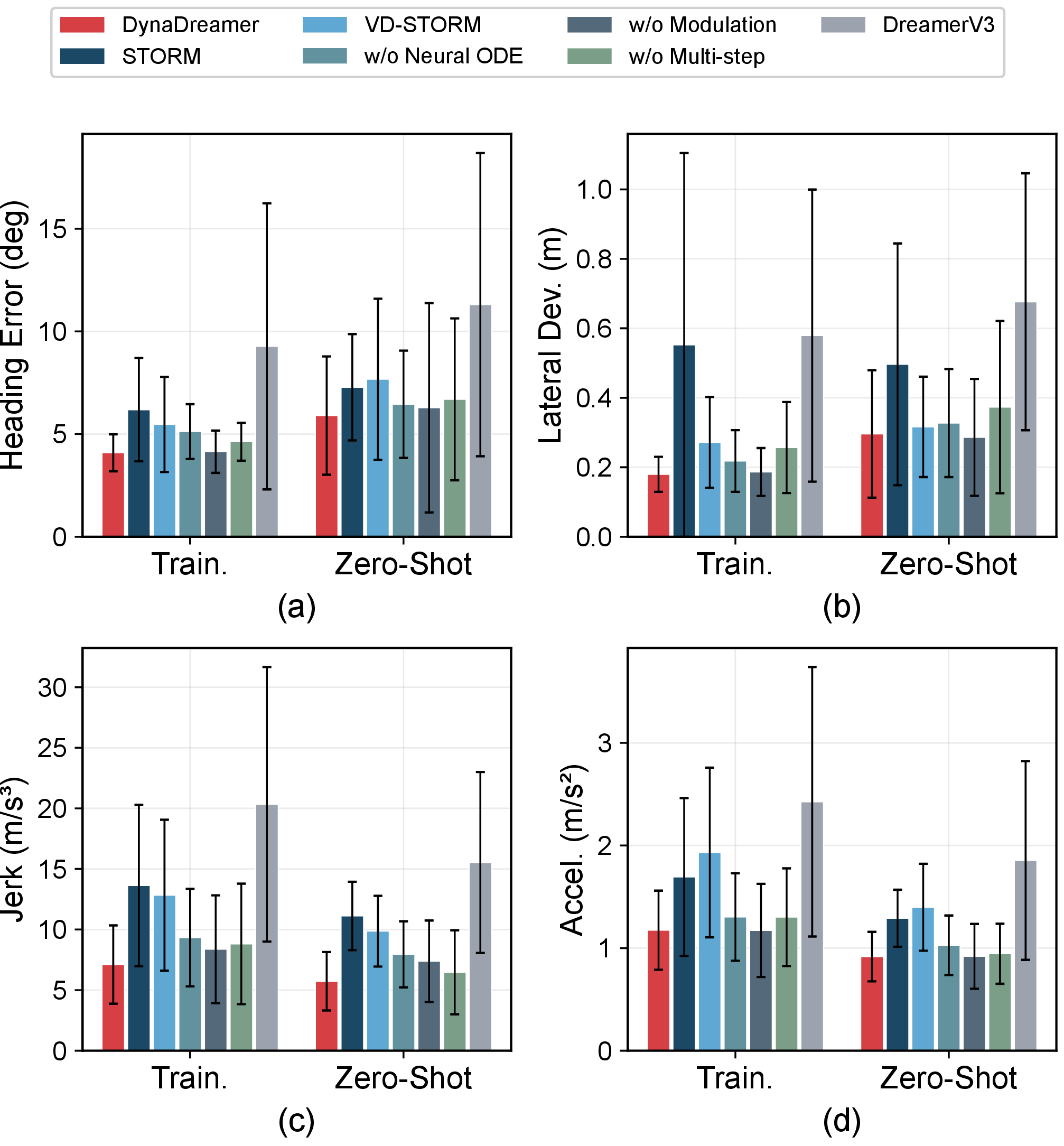
Figs. 6 and 7 provide complementary breakdowns of failure modes and driving quality on Town03. DynaDreamer exhibits balanced, low failure rates across all modes, whereas STORM and VD-STORM suffer from high out-of-lane rates (19.5% and 26.0%, respectively); ablation variants w/o Modulation and w/o Neural-ODE show elevated collision rates (17.5%), confirming that ego-dynamics augmentation is critical for safety. Among the three components, adaptive modulation has the strongest individual effect on task success rate. For driving quality, DynaDreamer achieves the lowest heading error and jerk, reflecting the smoothest trajectory following, and the radar chart in Fig. 6 (b) confirms its largest enclosed area, indicating the most well-balanced overall performance.
6.4 World Model Quality↩︎
Table 3 reports WM quality under pooled zero-shot evaluation (S2+S3), combining prior–posterior alignment (KL divergence) and BEV reconstruction (PSNR/MAE). DynaDreamer attains the lowest KL (10.62, vs. for DreamerV3 and 14.19 for STORM), the highest PSNR, and the lowest MAE, indicating both well-calibrated latent dynamics and faithful image generation. Ablation variants achieve comparable PSNR but consistently higher KL than DynaDreamer, suggesting that each component contributes to tightening the prior–posterior gap. Evaluated on unseen chassis (S2+S3), where the prior’s inability to anticipate ego-motion is most acute, this KL gap is the central empirical signature of Proposition 3. VD-STORM injects the ego-dynamics context only into the actor-critic while leaving the prior unconditioned, and attains a KL of 15.80, no better than STORM (14.19); routing the same context into the world model’s prior and posterior instead lowers the KL to 10.62. The monotonic decrease from STORM (14.19) through w/o Modulation (13.54, partial conditioning) to DynaDreamer (10.62, full AdaLN conditioning) further corroborates that the KL reduction scales with the degree to which the prior is informed of ego-dynamics.
| Method | KL\(_{\mathrm{prior\|post}}\) \(\downarrow\) | BEV PSNR (dB) \(\uparrow\) | BEV MAE \(\downarrow\) |
|---|---|---|---|
| DreamerV3 | 36.80 | 20.88 | 0.0337 |
| STORM | 14.19 | 22.53 | 0.0347 |
| VD-STORM | 15.80 | 23.24 | 0.0310 |
| w/o Neural-ODE | 13.67 | 23.24 | 0.0282 |
| w/o Modulation | 13.54 | 22.70 | 0.0345 |
| w/o Multi-step | 11.18 | 23.29 | 0.0298 |
| DynaDreamer | 10.62 | 23.55 | 0.0269 |
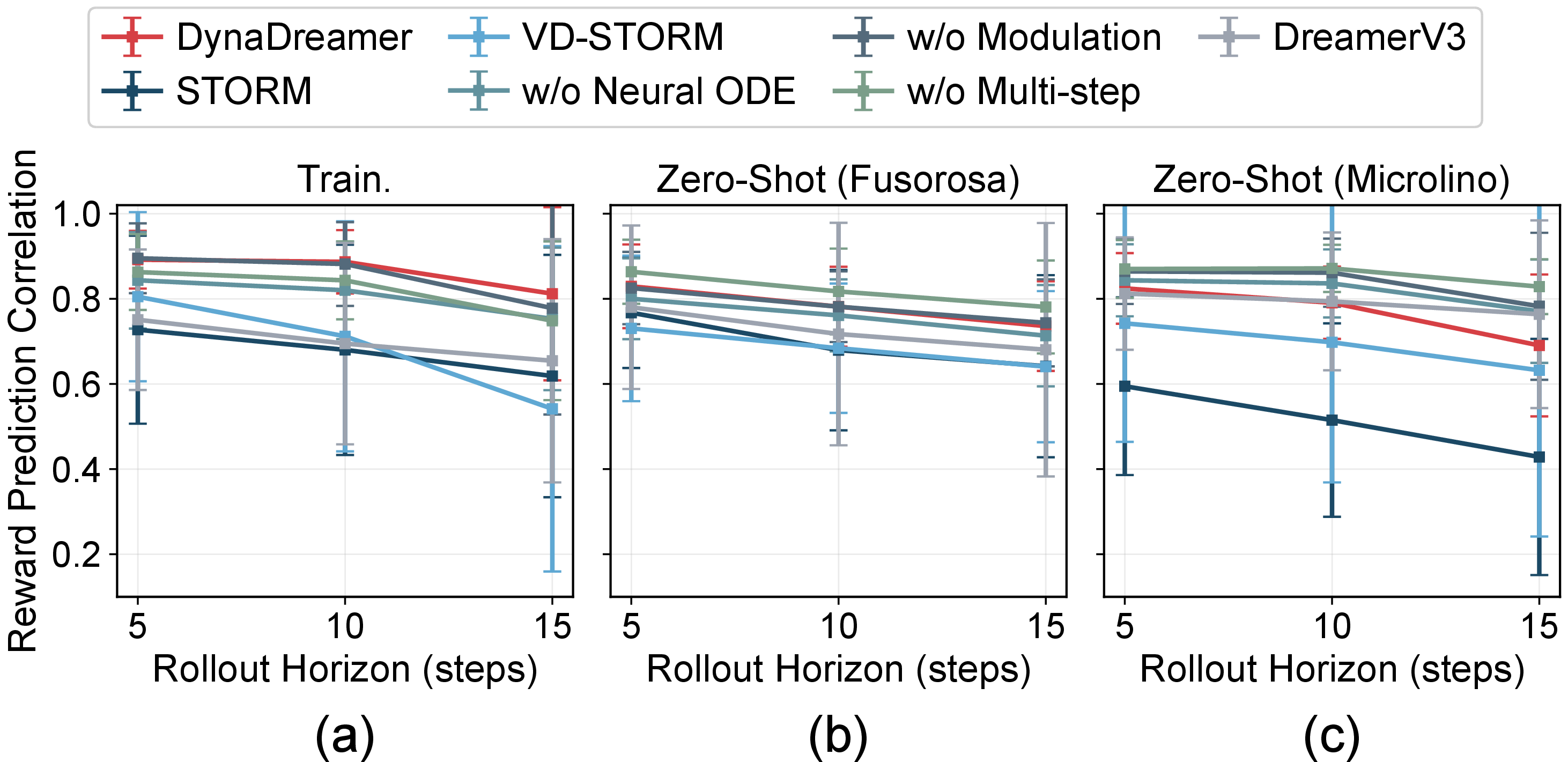
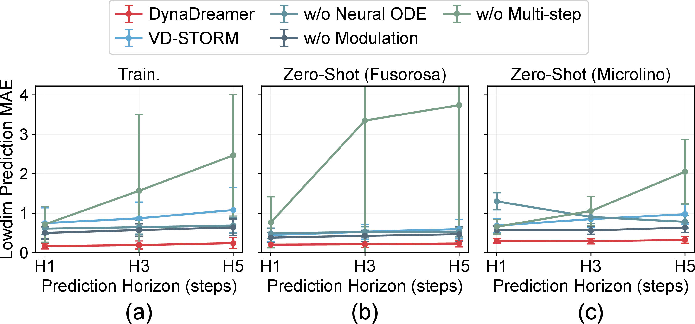
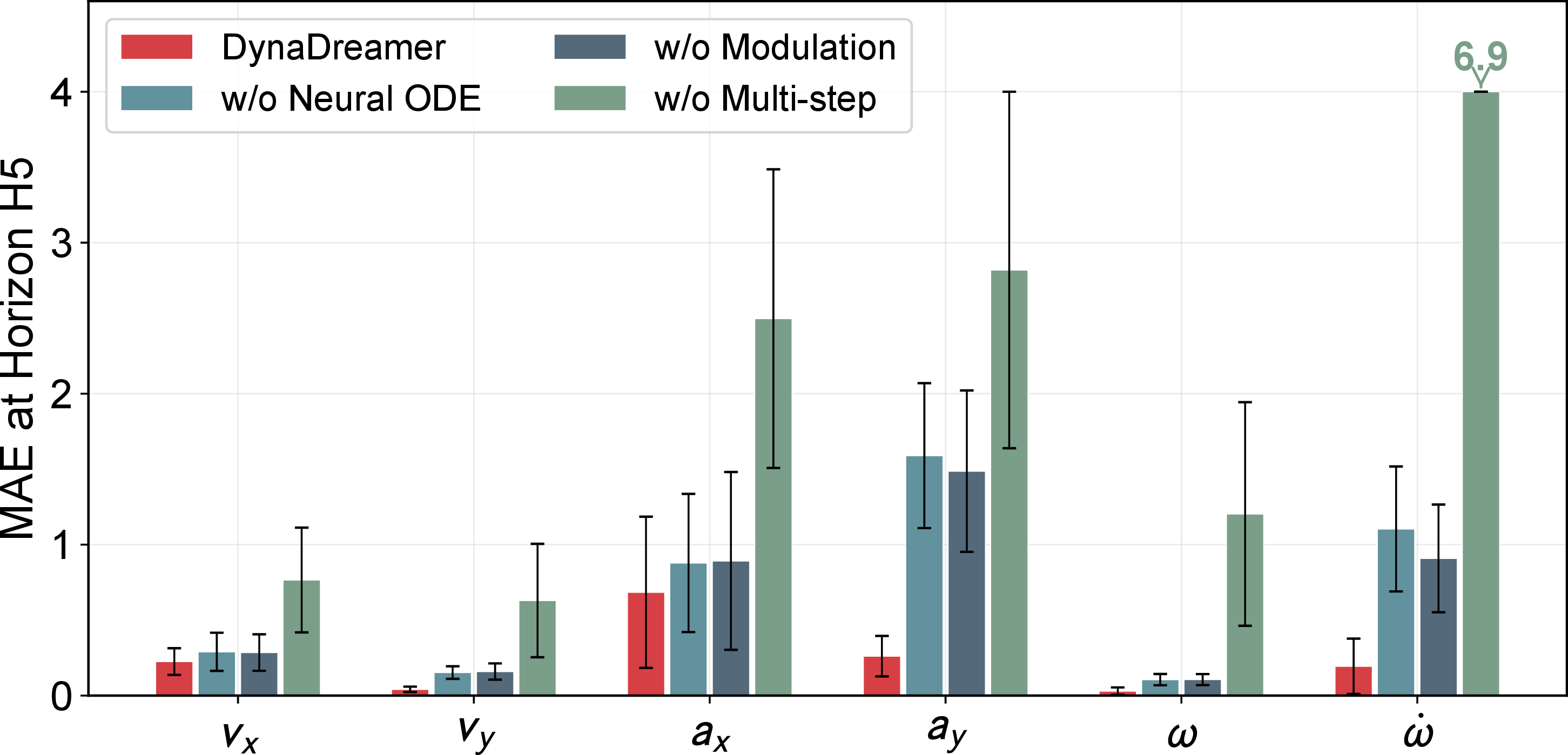
Figs. 8–10 further characterize imagination quality. DynaDreamer sustains the highest rollout reward correlation as the horizon grows. Its prediction error grows slowly from H1 to H5, whereas w/o Multi-step exhibits error explosion. This contrast highlights the practical importance of the drift bound in Corollary 1: multi-step supervision keeps \(\epsilon_{\mathrm{ode}}\) small, and refreshing \(\boldsymbol{\psi}_t\) along the rollout prevents ego-motion error from compounding. The per-component breakdown at H5 shows DynaDreamer excelling at lateral dynamics prediction, directly supporting lane-keeping performance. This advantage concentrates on the lateral and yaw components, which Eq. 19 attributes to the ego-induced warp. The burden isolated in Proposition 1 is therefore precisely the one the prior offloads.
The identifiability premise of Proposition 4 is examined directly through chassis parameter estimation. As shown in Table 4, DynaDreamer achieves the lowest estimation error and highest consistency, evidence that the ego-dynamics context \(\boldsymbol{\psi}_t\) is a sufficient statistic for the ego motion it must predict. VD-STORM performs comparably, consistent with its ego-dynamics prior, while w/o Multi-step shows noticeably degraded estimation, suggesting that multi-step auxiliary supervision provides useful gradient signals that also improve parameter learning. Table 5 provides a detailed per-parameter breakdown for DynaDreamer. The model accurately estimates diverse chassis parameters with relative errors ranging from 0.090 (steering limit) to 0.509 (moment of inertia). The higher error on \(I_z\) is expected given its large variance across vehicle types and its indirect observability from driving behavior alone.
| Method | Rel. Err. \(\downarrow\) | Log MSE \(\downarrow\) | Consist. \(\downarrow\) |
|---|---|---|---|
| VD-STORM | 1.527 | 0.910 | 1.019 |
| w/o Multi-step | 1.838 | 1.080 | 1.043 |
| DynaDreamer | 1.481 | 0.868 | 0.844 |
| Parameter | Ground Truth | Predicted | Rel. Err. |
|---|---|---|---|
| Mass (kg) | 3034 \(\pm\) 2710 | 2955 \(\pm\) 1759 | 0.329 |
| \(I_z\) (kg\(\cdot\)m\(^2\)) | 3700 \(\pm\) 6039 | 3437 \(\pm\) 3337 | 0.509 |
| \(C_f\) (kN/rad) | 93.3 \(\pm\) 62.2 | 80.0 \(\pm\) 38.6 | 0.331 |
| \(C_r\) (kN/rad) | 51.1 \(\pm\) 27.5 | 40.2 \(\pm\) 16.4 | 0.255 |
| \(l_f\) (m) | 1.17 \(\pm\) 0.37 | 1.12 \(\pm\) 0.24 | 0.153 |
| \(l_r\) (m) | 2.07 \(\pm\) 0.56 | 2.25 \(\pm\) 0.43 | 0.120 |
| \(\delta_{\max}\) (\(^\circ\)) | 70.0 \(\pm\) 5.5 | 64.4 \(\pm\) 0.6 | 0.090 |
6.5 Case Study↩︎
We present a case study on a zero-shot rollout of the 707 kg Microlino subcompact (roughly half the mass of the lightest training vehicle) and contrast STORM with DynaDreamer on a roundabout task. A supplementary Fusorosa bus rollout probes the opposite mass extreme in the parameter-identification case.
6.5.1 Qualitative Trajectory and Control Behavior↩︎
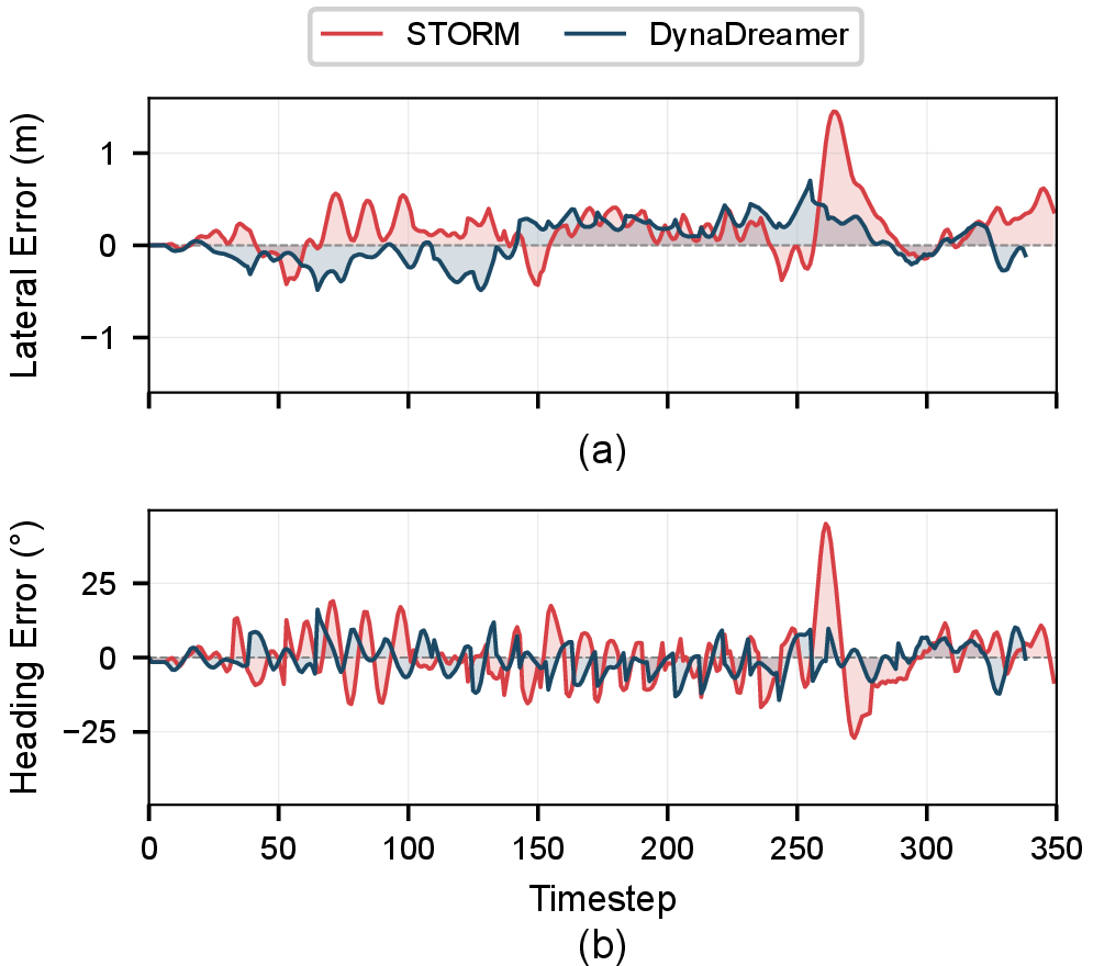
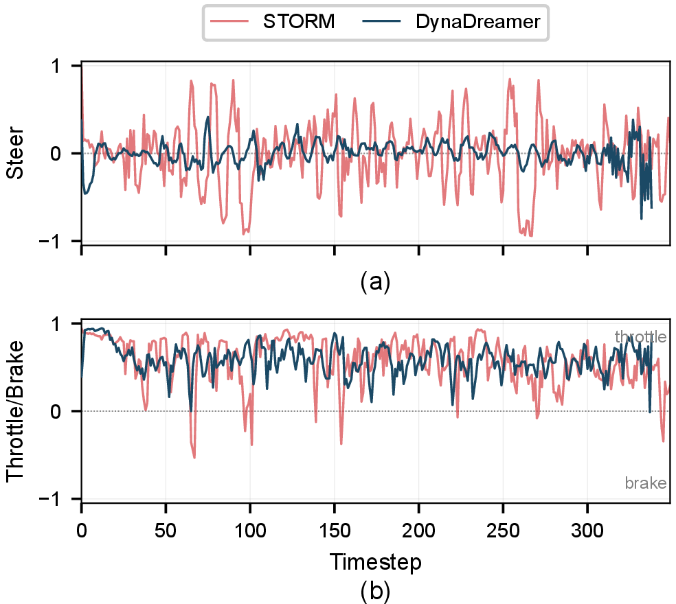
Fig. 11 plots signed lateral deviation and heading error. STORM remains biased to one side of the lane for 71% of the episode with a \(-1.45\) m peak excursion, whereas DynaDreamer oscillates symmetrically around the center line and stays within \(0.70\) m; heading error follows the same pattern, swinging up to \(\pm 45^\circ\) for STORM versus \(\pm 16^\circ\) for DynaDreamer. This tighter tracking yields the smoother control signals of Fig. 12: STORM issues saturating steer reversals and braking spikes, whereas DynaDreamer commits to low-gain commands throughout, consistent with its lowest jerk reported in Fig. 7. The root cause is representational: lacking an ego-dynamics prior, STORM cannot anticipate how its own steering warps the egocentric observation under the unfamiliar short-wheelbase chassis and resorts to over-correction. DynaDreamer’s prior supplies this warp in advance, enabling the symmetric, low-gain tracking above.
6.5.2 Low-Dimensional State Prediction and Parameter Identification↩︎
DynaDreamer’s smooth behavior stems from its Neural-ODE module. Fig. 13 overlays all six predicted dynamic states against ground truth; predictions remain aligned over the entire episode, including high-frequency lateral and yaw content, making their fidelity the proximate cause of the control quality above.
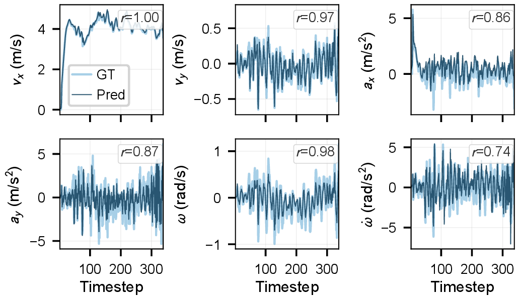
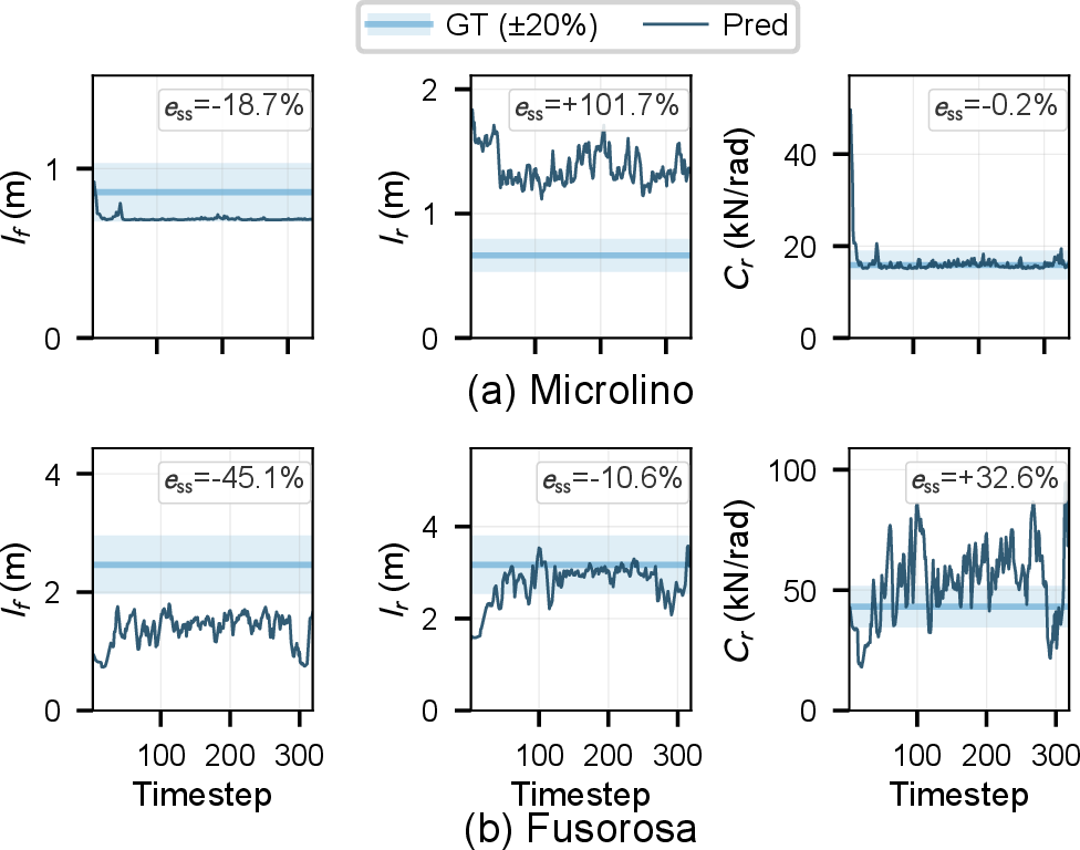
Fig. 14 traces zero-shot identification across both chassis extremes for a representative cross-section of the parameter vector: the two geometric terms \((l_f, l_r)\) and the rear cornering stiffness \(C_r\). We report this triplet as a representative sample: it spans both the geometric and the lateral-force parameter groups and reflects the typical parameter identification behavior. The two geometric terms settle near the ground truth with moderate steady-state bias, and \(C_r\) tracks the ground-truth trend with a residual offset. Such residuals are expected because vehicle parameters are tightly coupled in the bicycle model. This does not impair control significantly, as the parameter head is auxiliary and the neural residual absorbs such parameter bias, enabling DynaDreamer to generalize across the full mass range as shown in Table 4.
7 Conclusion↩︎
This paper formalizes the structural information bottleneck in BEV-based WM learning and introduces DynaDreamer to resolve it by supplying ego-motion as an explicit prior rather than leaving it to be inferred from statistics. The theoretical and empirical results converge on a broader conclusion: in egocentric WMs, any observation transition component that is exogenous and deterministic given a known context could be treated as a structural prior rather than reconstructed from pixels. Ego-motion in autonomous driving is the most prominent instance, and the principle may extend to other egocentric domains such as drone navigation or legged locomotion, where the agent’s own motion dominates the observation flow.
Two directions are particularly promising. First, extending the ego-dynamics prior to multi-agent imagination, where each surrounding traffic participant carries its own dynamics context, would enable traffic-aware closed-loop planning with per-agent physical plausibility. Second, sim-to-real deployment with online ego-dynamics adaptation would test whether the identified chassis parameters remain accurate under real-world sensor noise and actuator delay, bringing the demonstrated benefits closer to practical deployment.
References↩︎
This work was supported in part by Nanyang Technological University. (Corresponding author: Chen Lv.)↩︎
Zhidong Wang, Jingsong Liang, Zirui Li, Zhan Chen and Chen Lv are with the School of Mechanical and Aerospace Engineering, Nanyang Technological University, Singapore (e-mail:
zhidong001@e.ntu.edu.sg;jingsong002@e.ntu.edu.sg;zirui.li@ntu.edu.sg;zhan014@e.ntu.edu.sg;lyuchen@ntu.edu.sg).Zhidong Wang is also with the Collaborative Initiative, Interdisciplinary Graduate Programme, Nanyang Technological University, Singapore.
Han Yu is with the College of Computing and Data Science, Nanyang Technological University, Singapore (e-mail:
han.yu@ntu.edu.sg).↩︎