FM\(^2\): Unified Federated Foundation Models for Heterogeneous Multimodal Medical Imaging
July 15, 2026
Abstract
Building foundation models for medical imaging requires pooling data across institutions, yet privacy regulations prohibit centralized aggregation. Existing Federated Foundation Models either fine-tune natural-image models with poor medical-domain transfer, or train from scratch within a single modality, lacking the flexibility to unify tasks. We identify an under-explored challenge, Imaging Modality Heterogeneity, where clients operate under two structural regimes: Overlapped (shared modalities with heterogeneous label distributions) and Non-overlapped (fully disjoint modalities per client). We propose FM\(^2\), a unified framework that trains the core backbone from scratch to preserve medical domain fidelity while optionally incorporating biomedical pretrained encoders for vision-language alignment. FM\(^2\) equips each client with dual Mixture-of-Experts modules (a Class-wise MoE for personalized category knowledge and a Domain-wise MoE for shared cross-modality representations), coupled with a Heterogeneous Modality Alignment (HMA) regularizer that explicitly aligns modality-specific expert parameters, admitting provable \({\mathcal{O}}(1/\sqrt{T})\) convergence and generalization guarantees. FM\(^2\) further incorporates Caption-Enhanced Learning (CEL), where locally retained GPT-4o-generated captions serve as a textual semantic bridge enabling representation transfer across clients with disjoint modalities, and demonstrates extensibility to Federated Medical VQA. Experiments on our MIMH benchmark (classification and CEL) and real-world medical VQA datasets confirm consistent superiority over state-of-the-art federated baselines and strong out-of-modality generalization across all three tasks.
<ccs2012> <concept> <concept_id>10010147.10010178.10010224</concept_id> <concept_desc>Computing methodologies Computer vision</concept_desc> <concept_significance>500</concept_significance> </concept> <concept> <concept_id>10010147.10010257</concept_id> <concept_desc>Computing methodologies Machine learning</concept_desc> <concept_significance>500</concept_significance> </concept> </ccs2012>
1 Introduction↩︎
Foundation Models (FMs) have demonstrated remarkable cross-domain generalization by training large-scale architectures that integrate multiple domain-specific sub-models [1]. In medical imaging, building such FMs requires pooling numerous datasets from diverse institutions. However, strict privacy regulations such as GDPR [2] and HIPAA [3] prohibit the centralized aggregation of sensitive clinical data, creating a fundamental tension between model capability and data governance. Federated Foundation Models (FFMs) [4] resolve this tension by enabling collaborative training across institutions without exposing raw data, making them a natural paradigm for privacy-preserving medical AI.
Recent FFMs for medical imaging predominantly fine-tune pretrained natural-image models, including ViT [5], CLIP [6], and SAM [7], on medical downstream tasks. Liu et al. [8] fine-tuned SAM for federated medical image segmentation; Wu et al. [9] adapted CLIP for federated classification. Despite their convenience, these methods inherit a critical limitation: empirical evidence [10] shows that natural-image representations transfer poorly to the medical domain, where subtle inter-class variations, acquisition noise, and precise anatomical context demand domain-native knowledge that pretrained features cannot provide.
An alternative line of work trains FFMs from scratch on curated medical data [11], [12], acquiring richer domain-specific representations, echoing evidence from other modalities that federating the from-scratch training of a foundation model can match centralized counterparts while neutralizing per-domain bias [13]. Yet these efforts target single imaging modalities and single tasks. Real-world clinical AI demands a unified framework that simultaneously handles classification, caption-supervised representation learning, and visual question answering across heterogeneous modalities, under both Overlapped configurations (clients share modalities but with non-IID label distributions) and Non-overlapped configurations (each client holds a completely disjoint modality). Existing federated frameworks address at most a subset of these requirements. The compounding of classical data heterogeneity (non-IID labels) with Imaging Modality Heterogeneity, where feature distributions, noise characteristics, and semantic granularity differ fundamentally across clients, makes standard personalized FL methods, designed for label skew alone, insufficient for this setting.
This paper proposes FM\(^2\) (Federated Medical Multimodal foundation model), a framework that trains from scratch under Imaging Modality Heterogeneity and extends them to multimodal medical understanding. The core of FM\(^2\) is a dual Mixture-of-Experts (MoE) architecture: a Class-wise MoE retains personalized per-category knowledge locally, while a Domain-wise MoE captures shared cross-modality representations that are globally aggregated. A Heterogeneous Modality Alignment regularizer constrains the domain-wise experts toward global consensus, for which we prove a convergence rate of \({\mathcal{O}}(1/\sqrt{T})\) and an explicit generalization bound. Beyond classification, FM\(^2\) supports two multimodal extensions: (i) Caption-Enhanced Learning (CEL), where GPT-4o-generated captions (retained locally for privacy) provide federated vision-language contrastive supervision, serving as a shared semantic bridge that enriches representations even across clients with disjoint visual modalities; and (ii) Federated Medical VQA, demonstrating FM\(^2\)’s extensibility to natural-language querying of medical images across institutions. Our contributions are summarized as follows:
We formalize Imaging Modality Heterogeneity under both Overlapped and Non-overlapped modality regimes, and propose FM\(^2\), the first unified multi-task federated framework addressing both settings simultaneously.
We design dual MoE modules with a Heterogeneous Modality Alignment regularizer targeting modality-specific expert drift, and prove \({\mathcal{O}}(1/\sqrt{T})\) convergence and an explicit generalization bound (Theorem 1–Proposition 2).
We introduce Caption-Enhanced Learning (CEL), where locally retained GPT-4o captions provide a shared textual bridge: language descriptions share a common vocabulary across modalities, enabling representation transfer even when clients hold entirely disjoint visual domains.
We construct the MIMH benchmark (five modalities, four configurations) for federated Classification and Caption Enhanced Learning, and additionally evaluate on real-world medical VQA datasets for Federated Medical VQA, confirming consistent superiority across all three tasks with strong out-of-modality generalization.
2 Related Work↩︎
2.0.0.1 Heterogeneous Federated Learning.
FL trains models collaboratively across decentralized clients without exposing raw data [14]. Statistical heterogeneity (non-IID distributions) is a central challenge: naive aggregation causes client drift and degraded convergence. Personalized FL (PFL) addresses this through several families of techniques. Regularization-based methods [15], [16] add proximal penalties to keep local models close to the global reference while permitting per-client drift; Ditto [16] exemplifies this by solving a personalized objective with a global proximal term, and FFTS [17] extends the idea to foundation models by regularizing both client and server side to align knowledge across statistically heterogeneous datasets. Partial-sharing methods split the network into a globally aggregated backbone and a local task-specific head: FedBN [18] keeps batch normalization layers local to absorb feature shift, FedRep [19] retains only the classifier locally, and prompt- or adapter-based approaches [20], [21] share only lightweight parameters while keeping the backbone on-device. Adaptive aggregation [22] weights client contributions by similarity, and meta-learning methods such as Per-FedAvg [23] learn a shared initialization that enables rapid per-client fine-tuning. Despite their diversity, all of these approaches assume a homogeneous feature space and optimize for a single task, making them unsuitable when clients differ fundamentally in imaging modality. Mixture-of-experts approaches have also been explored in FL [24], [25], yet none disentangle class-level from modality-level heterogeneity simultaneously; centralized missing-modality strategies [26] are further inapplicable since FL prohibits raw cross-site feature aggregation.
2.0.0.2 FL for Medical Images.
Federated learning has been applied to privacy-preserving medical image classification [27]–[30] and, more recently, to vision-language tasks including medical VQA [31], [32]. For classification, methods such as FedFMS [8] and FedTCA [33] are typically task-specific and backbone-dependent, requiring re-engineering for each setting and assuming a single shared imaging modality. For vision-language understanding, FedDAT [34], PromptFL [35], and F\(^3\)OCUS [36] adapt pretrained VLMs to federated settings via dual adapters, prompt tuning, and client-layer meta-learning, but remain confined to single-modality client scenarios. No existing method jointly supports classification and VQA under a protocol that handles cross-modality structure. FM\(^2\) fills this gap by disentangling class-level personalization from modality-level consensus via dual MoE modules, enabling unified multi-task training across heterogeneous imaging modalities without task-specific re-engineering.
3 Methodology↩︎
3.1 Overview↩︎
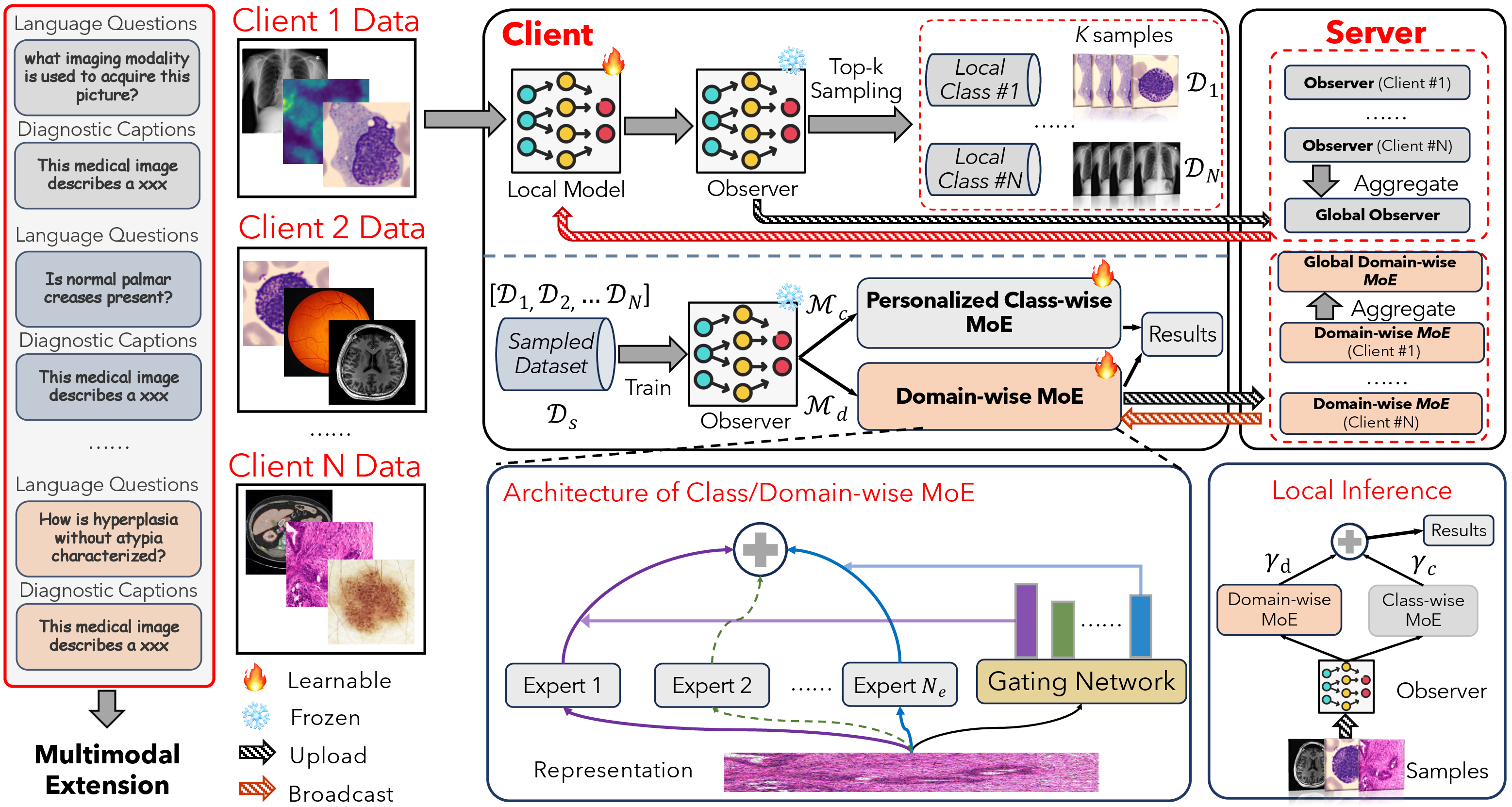
Fig. 1 illustrates the FM\(^2\) framework. Each client first trains a local visual encoder \({\mathcal{F}}(\cdot) = \{{\mathcal{F}}_b, {\mathcal{F}}_h\}\) on its own data. The backbone \({\mathcal{F}}_b\) then serves as a frozen Observer \({\mathcal{V}}\) that performs Top-\(K\) Sampling to extract representative subsets \({\mathcal{D}}_1, \ldots, {\mathcal{D}}_N\) per class, forming a sampled dataset \({\mathcal{D}}_s = \bigcup_{i=1}^N {\mathcal{D}}_i\). Two MoE modules, namely Class-wise MoE \({\mathcal{M}}_c\) and Domain-wise MoE \({\mathcal{M}}_d\), are trained on \({\mathcal{D}}_s\) following \({\mathcal{V}}\). After local updates, \({\mathcal{V}}\) and \({\mathcal{M}}_d\) are uploaded for global aggregation; \({\mathcal{M}}_c\) remains local for personalization. \({\mathcal{V}}\) is frozen during stage-2 MoE training but uploaded at round end so the server can aggregate and redistribute a refined backbone for the next round’s stage-1 initialization. For multimodal extension, an optional text encoder \({\mathcal{T}}\) processes expert-generated captions, and a VQA head \({\mathcal{H}}_{\text{vqa}}\) enables question answering, both sharing the same MoE-enhanced visual backbone.
3.2 Dual Mixture-of-Experts for Heterogeneity↩︎
3.2.0.1 Observer and Top-\(K\) Sampling.
In the first training stage, each client trains its local model \({\mathcal{F}}\) with labeled images. The trained backbone, designated as the Observer \({\mathcal{V}}= {\mathcal{F}}_b\), computes a representativeness score \(S = \texttt{Sigmoid}({\mathcal{V}}({\boldsymbol{X}}_z))\) for each class \(z\). Top-\(K\) Sampling selects the \(K\) highest-scoring samples per class, forming subsets \({\mathcal{D}}_1, \ldots, {\mathcal{D}}_N\) (sensitivity analysis of \(K\) in Appendix B). This observer-guided selection addresses local label drift by ensuring that only the most informative samples enter the second stage.
3.2.0.2 Class-wise MoE (CMoE)
To handle label heterogeneity, the CMoE \({\mathcal{M}}_c\) allocates \(N_c\) experts (one per local class, \(N_c = N\)), each specializing in class-specific feature transformations: \[\label{eq:cmoe} \hat{{\boldsymbol{X}}} = \sum_{{\mathbf{n}}=1}^{N_c} W_{{\mathbf{n}}} \cdot E_{{\mathbf{n}}}({\boldsymbol{X}}_{\text{mid}}),\quad \text{where}\; E({\boldsymbol{X}}_{\text{mid}}) = \mathrm{\small ReLU}(\mathrm{\small MLP}({\boldsymbol{X}}_{\text{mid}})),\tag{1}\] where \({\boldsymbol{X}}_{\text{mid}}\) and \(\hat{{\boldsymbol{X}}}\) denote latent and output representations, \(E_{{\mathbf{n}}}\) is the \({\mathbf{n}}\)-th expert network, and \(W_{{\mathbf{n}}}\) is the gating weight. By decomposing the representation space into class-specific subspaces, CMoE transforms the classification problem into learning multiple potential class-specific knowledge bases, each tailored to the client’s local label distribution. The CMoE remains on each client and is never uploaded, preserving personalization.
3.2.0.3 Domain-wise MoE (DMoE)
To handle modality heterogeneity, the DMoE \({\mathcal{M}}_d\) allocates \(N_d\) experts (one per imaging modality), each capturing modality-specific feature transformations. Its architecture mirrors CMoE but with experts indexed by imaging domain rather than class. Expert indices are pre-assigned via a shared global modality vocabulary declared at federation setup, reflecting the practical assumption that each clinical site knows its imaging modality (e.g., a radiology department knows it operates CT scanners); extension to unknown-modality scenarios via online feature clustering is discussed in Appendix C. The DMoE is globally aggregated, enabling cross-client knowledge transfer of domain representations.
For inference, the final prediction combines both MoE modules: \[\label{eq:eq2} y = \gamma_d \cdot {\mathcal{M}}_d({\mathcal{V}}({\boldsymbol{X}})) + \gamma_c \cdot {\mathcal{M}}_c({\mathcal{V}}({\boldsymbol{X}})),\tag{2}\] where \(\gamma_d, \gamma_c \in [0,1]\) with \(\gamma_d + \gamma_c = 1\) balance domain consensus and personalized expertise.
3.3 Heterogeneous Modality Alignment↩︎
Aggregating domain-wise experts across clients with fundamentally different imaging modalities risks introducing consensus bias. We mitigate this through a regularization that explicitly constrains the local DMoE parameters \({\mathcal{M}}_d^i\) toward the global aggregate \(\hat{{\mathcal{M}}}_d\): \[\label{eq:optimization} \begin{align} &\min_{\{\theta_1, \ldots, \theta_Z\}} \sum_{i=1}^Z \frac{n_i}{n} \bigl[{\mathcal{L}}_i(\theta_i;{\mathcal{D}}^i, {\mathcal{D}}_s^i) + \lambda \|{\mathcal{M}}_d^i - \hat{{\mathcal{M}}}_d\|^2\bigr], \\ &\text{s.t.}\quad \hat{{\mathcal{M}}}_d = \mathop{\mathrm{arg\,min}}_{{\mathcal{M}}_d} G({\mathcal{M}}_d^1, \ldots, {\mathcal{M}}_d^Z), \\ &\text{where}\quad {\mathcal{L}}_i(\theta_i;{\mathcal{D}}^i, {\mathcal{D}}_s^i) = -\sum_{c=1}^C y_c \log(\hat{y}_i(x)),\; \theta_i = \{{\mathcal{V}}^i, {\mathcal{M}}_d^i, {\mathcal{M}}_c^i\}. \end{align}\tag{3}\] Here \(\lambda > 0\) controls the alignment strength, \(n_i / n\) weights clients by data volume, and \(\hat{{\mathcal{M}}}_d\) is obtained via FedAvg. The proximal term \(\lambda\|{\mathcal{M}}_d^i - \hat{{\mathcal{M}}}_d\|^2\) serves two purposes: it prevents local domain experts from drifting too far from the global consensus while still allowing modality-specific adaptation. Unlike FedProx [37] and Ditto [16], which apply a global proximal penalty to the entire model, HMA constrains only the DMoE parameters, exploiting the dual-MoE structure to selectively align modality-specific representations while leaving CMoE fully free for per-client personalization. We establish formal convergence guarantees for this in Sec. 3.5.
3.4 Multimodal Extensions↩︎
The dual MoE architecture provides a modality-aware visual backbone that naturally supports richer output modalities beyond classification. We introduce two extensions that operate on the same MoE-enhanced features without modifying the core framework.
3.4.0.1 Caption-Enhanced Learning (CEL)
Medical images encode rich diagnostic information that class labels alone cannot capture, such as lesion morphology, tissue texture, and spatial relationships. This limitation is particularly acute in the Non-overlapped setting (MIMH-SA), where clients hold entirely disjoint imaging modalities: visual feature distributions share no common structure across clients, yet their textual descriptions share a common diagnostic vocabulary regardless of modality. CEL exploits this asymmetry by aligning local visual features with LLM-generated captions through a federated contrastive objective, so that language serves as a shared semantic bridge enabling cross-client representation transfer even when visual domains are completely disjoint. To inject this knowledge, we generate diagnostic captions for each image in the MIMH dataset using GPT-4o [38] via a ReAct-based [39] agent pipeline (full prompts and quality-filtering criteria in Appendix D) in a zero-shot setting (e.g., “Fundus image showing microaneurysms and hard exudates in the macular region, consistent with moderate non-proliferative diabetic retinopathy”). A lightweight text encoder \({\mathcal{T}}\) (PubMedBERT [40]) extracts caption embeddings \({\boldsymbol{t}}= {\mathcal{T}}(\text{caption})\), which are aligned with the visual features \({\boldsymbol{v}}= {\mathcal{V}}({\boldsymbol{X}})\) through the federated contrastive objective: \[\label{eq:cel} {\mathcal{L}}_{\text{CEL}} = -\frac{1}{B}\sum_{j=1}^{B} \log \frac{\exp(\text{sim}({\boldsymbol{v}}_j, {\boldsymbol{t}}_j) / \tau)}{\sum_{k=1}^{B} \exp(\text{sim}({\boldsymbol{v}}_j, {\boldsymbol{t}}_k) / \tau)},\tag{4}\] where \(\text{sim}(\cdot, \cdot)\) denotes cosine similarity, \(\tau\) is a temperature parameter, and \(B\) is the batch size. The total local objective becomes \({\mathcal{L}}_i + \alpha \cdot {\mathcal{L}}_{\text{CEL}}\), where \(\alpha\) balances classification and contrastive losses. Crucially, \({\mathcal{L}}_{\text{CEL}}\) enriches the Observer’s representations with fine-grained semantic structure without requiring caption data to leave the client, preserving privacy. The text encoder parameters remain local; only the visual backbone and DMoE are aggregated.
3.4.0.2 Federated Medical VQA
To demonstrate FM\(^2\)’s capacity for multimodal reasoning, we extend it to Visual Question Answering on medical images. Given an image \({\boldsymbol{X}}\) and a natural-language question \(q\), we extract visual features \({\boldsymbol{v}}= {\mathcal{M}}_d({\mathcal{V}}({\boldsymbol{X}})) \oplus {\mathcal{M}}_c({\mathcal{V}}({\boldsymbol{X}}))\) (where \(\oplus\) denotes concatenation weighted by \(\gamma_d, \gamma_c\)) and question features \({\boldsymbol{q}}= {\mathcal{T}}_q(q)\) via a question encoder \({\mathcal{T}}_q\). A lightweight answer module \({\mathcal{H}}_{\text{vqa}}\) fuses both: \[\label{eq:vqa} a = {\mathcal{H}}_{\text{vqa}}({\boldsymbol{v}}\odot {\boldsymbol{q}}),\tag{5}\] where \(\odot\) denotes element-wise gating. The VQA loss \({\mathcal{L}}_{\text{VQA}}\) (binary cross-entropy over candidate answers) is added to the local objective. The DMoE’s domain-specific experts naturally handle modality-dependent questions (e.g., questions about retinal layers vs.tissue staining), while the CMoE provides category-aware visual reasoning. The question encoder and answer head are locally trained; the shared visual backbone benefits from federated aggregation across all tasks.
3.5 Theoretical Analysis↩︎
We provide convergence and generalization guarantees for the FM\(^2\) optimization defined in Eq. 3 . For clarity, we write the global objective as \(F(\theta) = \sum_{i=1}^Z \frac{n_i}{n}\bigl[{\mathcal{L}}_i(\theta_i) + \lambda\|{\mathcal{M}}_d^i - \hat{{\mathcal{M}}}_d\|^2\bigr]\), where each client’s alignment penalty is included inside the per-client term.
Assumption 1. Each local loss \({\mathcal{L}}_i(\theta)\) is \(L\)-smooth: \(\|\nabla {\mathcal{L}}_i(\theta) - \nabla {\mathcal{L}}_i(\theta')\| \leq L\|\theta - \theta'\|\) for all \(\theta, \theta'\). As the alignment penalty is quadratic with curvature \(2\lambda\), \(F\) is \((L{+}2\lambda)\)-smooth; we absorb this into \(L\) for brevity.
Assumption 2. The stochastic gradient \(g_i\) at client \(i\) is unbiased, \(\mathbb{E}[g_i] = \nabla {\mathcal{L}}_i(\theta)\), satisfies \(\mathbb{E}\|g_i - \nabla {\mathcal{L}}_i(\theta)\|^2 \leq \sigma^2\), and its noise is independent across clients.
Assumption 3. The modality heterogeneity is bounded: \[\textstyle\frac{1}{Z}\sum\nolimits_{i=1}^Z \|\nabla {\mathcal{L}}_i(\theta) - \nabla F(\theta)\|^2 \leq \delta^2.\]
Theorem 1 (Convergence of FM\(^2\)). Under Assumptions 1–3, with learning rate \(\eta \leq \min\{1/(4L),\,1/(2\lambda)\}\) and alignment parameter \(\lambda > 0\), after \(T\) communication rounds of FM\(^2\), the averaged squared gradient norm satisfies: \[\label{eq:convergence} \begin{align} \frac{1}{T}\sum_{t=0}^{T-1} \mathbb{E}\|\nabla F(\theta^t)\|^2 \leq\; & \underbrace{\frac{2(F(\theta^0) - F^*)}{\eta T}}_{\text{init.\;gap}} + \underbrace{\frac{4L\eta\sigma^2}{Z}}_{\text{stoch.\;noise}} \\ & + \underbrace{4L\eta\delta^2}_{\text{heterogeneity}} + \underbrace{\frac{2\lambda L \Delta_{{\mathcal{M}}}}{T}}_{\text{align.\;drift}}, \end{align}\qquad{(1)}\] where \(F^* = \inf_\theta F(\theta)\) and \(\Delta_{{\mathcal{M}}} = \max_i \|{\mathcal{M}}_d^{i,0} - \hat{{\mathcal{M}}}_d^0\|^2\) is the initial modality divergence.
Proof. By the \(L\)-smoothness of \({\mathcal{L}}_i\) (Assumption 1), the global objective \(F\) satisfies: \[\label{eq:descent} F(\theta^{t+1}) \leq F(\theta^t) + \langle \nabla F(\theta^t), \theta^{t+1} - \theta^t \rangle + \frac{L}{2}\|\theta^{t+1} - \theta^t\|^2.\tag{6}\] Substituting the update \(\theta^{t+1} = \theta^t - \eta \bar{g}^t\), where \(\bar{g}^t = \sum_{i=1}^Z p_i\bigl[g_i^t + 2\lambda({\mathcal{M}}_d^{i,t} - \hat{{\mathcal{M}}}_d^t)\bigr]\) with \(p_i = n_i/n\) is the aggregated gradient including the alignment term, we obtain: \[F(\theta^{t+1}) \leq F(\theta^t) - \eta \langle \nabla F(\theta^t), \bar{g}^t \rangle + \frac{L\eta^2}{2}\|\bar{g}^t\|^2.\] Taking expectation and decomposing \(\mathbb{E}\|\bar{g}^t\|^2\), we bound the variance term using Assumption 2: \(\mathbb{E}\|\bar{g}^t - \nabla F(\theta^t)\|^2 \leq \sigma^2/Z + \delta^2 + 4\lambda^2 \Delta_{{\mathcal{M}}}^t\), where \(\Delta_{{\mathcal{M}}}^t = \frac{1}{Z}\sum_i \|{\mathcal{M}}_d^{i,t} - \hat{{\mathcal{M}}}_d^t\|^2\).
To control \(\Delta_{{\mathcal{M}}}^t\), observe that the gradient of the alignment penalty with respect to \({\mathcal{M}}_d^i\) is \(2\lambda({\mathcal{M}}_d^{i,t} - \hat{{\mathcal{M}}}_d^t)\). After the local gradient step, \({\mathcal{M}}_d^{i,t+1} = {\mathcal{M}}_d^{i,t} - 2\lambda\eta({\mathcal{M}}_d^{i,t} - \hat{{\mathcal{M}}}_d^t) - \eta \nabla_{{\mathcal{M}}_d^i}{\mathcal{L}}_i^t\). Since the server aggregate satisfies \(\hat{{\mathcal{M}}}_d^{t+1} = \frac{1}{Z}\sum_i {\mathcal{M}}_d^{i,t+1}\), the residual \({\mathcal{M}}_d^{i,t+1} - \hat{{\mathcal{M}}}_d^{t+1} = (1-2\lambda\eta)({\mathcal{M}}_d^{i,t} - \hat{{\mathcal{M}}}_d^t) - \eta(\nabla_{{\mathcal{M}}_d^i}{\mathcal{L}}_i^t - \overline{\nabla{\mathcal{L}}}^t)\). Taking norms, averaging, and applying Young’s inequality with \(\beta = 2\lambda\eta/(1-2\lambda\eta)\) yields \(\Delta_{{\mathcal{M}}}^{t+1} \leq (1-2\lambda\eta)\Delta_{{\mathcal{M}}}^t + \frac{\eta}{2\lambda}\delta^2\), where \(2\lambda\eta \leq 1\) holds because \(\eta \leq 1/(2\lambda)\). Telescoping gives \(\frac{1}{T}\sum_{t=0}^{T-1}\Delta_{{\mathcal{M}}}^t \leq \frac{\Delta_{{\mathcal{M}}}}{2\lambda\eta T} + \frac{\delta^2}{4\lambda^2}\); the second term enters the bound as \({\mathcal{O}}(L\eta\delta^2)\) and is absorbed into the heterogeneity term, while the first, scaled by the \(4\lambda^2\) coefficient and the \(L\eta\) prefactor of the variance, contributes \(2\lambda L \Delta_{{\mathcal{M}}}/T\).
Combining, using \(\eta \leq 1/(4L)\), and telescoping over \(T\) rounds: \[\frac{1}{T}\sum_{t=0}^{T-1} \mathbb{E}\|\nabla F(\theta^t)\|^2 \leq \frac{2(F(\theta^0) - F^*)}{\eta T} + \frac{4L\eta\sigma^2}{Z} + 4L\eta\delta^2 + \frac{2\lambda L \Delta_{{\mathcal{M}}}}{T}.\] Setting \(\eta = {\mathcal{O}}(1/\sqrt{T})\) yields the overall convergence rate \({\mathcal{O}}(1/\sqrt{T})\). ◻
The bound shows that \(\sigma^2/Z\) diminishes with more clients; \(\delta^2\) captures modality heterogeneity reduced by dual MoE disentanglement; and \(2\lambda L\Delta_{{\mathcal{M}}}/T\) vanishes at \({\mathcal{O}}(1/T)\), confirming HMA progressively eliminates modality drift.
Proposition 2 (Generalization with Dual MoE). Let \(h = \gamma_d \cdot {\mathcal{M}}_d \circ {\mathcal{V}}+ \gamma_c \cdot {\mathcal{M}}_c \circ {\mathcal{V}}\) be the FM\(^2\) predictor, with \(\gamma_d, \gamma_c \geq 0\) and \(\gamma_d + \gamma_c = 1\) as in Eq. 2 . For any joint distribution \(P\) over images and labels with modality indicator \(m({\boldsymbol{X}})\) and any loss \(\ell \in [0,1]\) convex in its first argument, the expected risk admits the decomposition: \[\label{eq:generalization} R(h) \leq \gamma_d \cdot R_d^* + \gamma_c \cdot R_c^* + 2\sqrt{2\gamma_d \gamma_c\, d_{\mathrm{JS}}(P_d \| P_c)} + \epsilon_{{\mathcal{V}}},\qquad{(2)}\] where \(R_d^*\) and \(R_c^*\) are the Bayes-optimal risks of the domain-wise and class-wise experts respectively, \(d_{\mathrm{JS}}(\cdot\|\cdot)\) denotes the Jensen–Shannon divergence between the domain and class expert output distributions, and \(\epsilon_{{\mathcal{V}}}\) is the Observer’s approximation error.
| Dataset | Method | \(\varphi=0.1\) (Hard) | \(\varphi=0.3\) (Moderate) | \(\varphi=100\) (Easy) | ||||||||||||||||||||||||
|---|---|---|---|---|---|---|---|---|---|---|---|---|---|---|---|---|---|---|---|---|---|---|---|---|---|---|---|---|
| 3-5 (lr)6-8 (lr)9-11 | \(r = 30\%\) | \(r = 50\%\) | \(r = 100\%\) | \(r = 30\%\) | \(r = 50\%\) | \(r = 100\%\) | \(r = 30\%\) | \(r = 50\%\) | \(r = 100\%\) | |||||||||||||||||||
| 5-Domain | FedAvg | \(18.67_{(\pm0.30)}\) | \(29.68_{(\pm0.21)}\) | \(23.05_{(\pm0.47)}\) | \(33.06_{(\pm1.40)}\) | \(39.29_{(\pm0.20)}\) | \(36.43_{(\pm0.22)}\) | \(27.78_{(\pm0.29)}\) | \(34.47_{(\pm0.62)}\) | \(31.90_{(\pm0.92)}\) | ||||||||||||||||||
| FedProx | \(47.94_{(\pm0.23)}\) | \(34.99_{(\pm0.60)}\) | \(38.70_{(\pm0.12)}\) | \(33.61_{(\pm0.21)}\) | \(36.26_{(\pm0.05)}\) | \(39.53_{(\pm0.34)}\) | \(31.25_{(\pm0.34)}\) | \(35.70_{(\pm0.07)}\) | \(31.61_{(\pm0.79)}\) | |||||||||||||||||||
| PerFedAvg | \(29.42_{(\pm0.50)}\) | \(39.75_{(\pm0.51)}\) | \(50.91_{(\pm0.23)}\) | \(44.18_{(\pm0.29)}\) | \(38.52_{(\pm0.27)}\) | \(43.06_{(\pm0.52)}\) | \(29.51_{(\pm0.41)}\) | \(51.61_{(\pm0.39)}\) | \(44.71_{(\pm0.54)}\) | |||||||||||||||||||
| FedBN | \(25.95_{(\pm0.41)}\) | \(33.79_{(\pm0.81)}\) | \(42.72_{(\pm0.41)}\) | \(29.93_{(\pm0.47)}\) | \(39.33_{(\pm0.04)}\) | \(39.59_{(\pm0.06)}\) | \(24.79_{(\pm0.35)}\) | \(37.91_{(\pm0.28)}\) | \(35.01_{(\pm0.76)}\) | |||||||||||||||||||
| FedProto | \(42.49_{(\pm0.72)}\) | \(57.51_{(\pm0.26)}\) | \(70.84_{(\pm1.17)}\) | \(39.50_{(\pm0.13)}\) | \(45.09_{(\pm0.86)}\) | \(56.89_{(\pm0.49)}\) | \(52.78_{(\pm0.77)}\) | \(68.42_{(\pm0.17)}\) | \(85.00_{(\pm1.71)}\) | |||||||||||||||||||
| FedRep | \(66.97_{(\pm0.34)}\) | \(73.47_{(\pm0.29)}\) | \(74.72_{(\pm0.56)}\) | \(60.32_{(\pm1.28)}\) | \(65.63_{(\pm0.32)}\) | \(60.28_{(\pm0.61)}\) | \(52.87_{(\pm0.99)}\) | \(64.48_{(\pm0.47)}\) | \(62.01_{(\pm1.01)}\) | |||||||||||||||||||
| FM\(^2\)-Tiny | \(74.05_{(\pm0.74)}\) | \(79.21_{(\pm0.50)}\) | \(83.79_{(\pm0.45)}\) | \(63.03_{(\pm0.85)}\) | \(69.76_{(\pm0.26)}\) | \(63.73_{(\pm0.91)}\) | \(60.80_{(\pm0.14)}\) | \(73.36_{(\pm0.39)}\) | \(87.11_{(\pm0.58)}\) | |||||||||||||||||||
| FM\(^2\)-Medium | \(74.83_{(\pm 0.53)}\) | \(82.14_{(\pm 0.85)}\) | \(85.66_{(\pm 0.29)}\) | \(66.96_{(\pm 0.70)}\) | \(68.05_{(\pm 0.61)}\) | \(69.51_{(\pm 0.70)}\) | \(62.94_{(\pm 0.12)}\) | \(74.27_{(\pm 0.80)}\) | \(89.68_{(\pm 0.93)}\) | |||||||||||||||||||
| FM\(^2\)-Large | \(76.05_{(\pm 0.84)}\) | \(83.74_{(\pm 0.92)}\) | \(86.68_{(\pm 0.75)}\) | \(67.53_{(\pm 0.93)}\) | \(69.79_{(\pm 0.62)}\) | \(70.49_{(\pm 0.99)}\) | \(63.29_{(\pm 0.22)}\) | \(76.73_{(\pm 0.41)}\) | \(90.39_{(\pm 0.64)}\) | |||||||||||||||||||
| 4-Domain | FedAvg | \(29.79_{(\pm0.21)}\) | \(34.05_{(\pm0.02)}\) | \(43.81_{(\pm0.78)}\) | \(42.01_{(\pm0.30)}\) | \(49.81_{(\pm0.77)}\) | \(51.50_{(\pm1.26)}\) | \(27.59_{(\pm0.11)}\) | \(25.07_{(\pm0.78)}\) | \(30.80_{(\pm1.11)}\) | ||||||||||||||||||
| FedProx | \(28.78_{(\pm0.13)}\) | \(46.12_{(\pm0.41)}\) | \(40.33_{(\pm0.16)}\) | \(41.20_{(\pm0.45)}\) | \(47.75_{(\pm0.88)}\) | \(52.06_{(\pm0.65)}\) | \(27.41_{(\pm0.24)}\) | \(33.01_{(\pm0.26)}\) | \(30.06_{(\pm0.31)}\) | |||||||||||||||||||
| PerFedAvg | \(41.19_{(\pm0.12)}\) | \(42.59_{(\pm0.30)}\) | \(45.71_{(\pm0.10)}\) | \(56.56_{(\pm0.12)}\) | \(53.84_{(\pm0.79)}\) | \(58.64_{(\pm0.22)}\) | \(34.00_{(\pm0.31)}\) | \(33.31_{(\pm0.17)}\) | \(37.78_{(\pm0.88)}\) | |||||||||||||||||||
| FedBN | \(36.36_{(\pm0.09)}\) | \(47.32_{(\pm0.44)}\) | \(48.65_{(\pm0.09)}\) | \(40.38_{(\pm0.12)}\) | \(53.40_{(\pm0.31)}\) | \(55.77_{(\pm1.23)}\) | \(21.22_{(\pm0.31)}\) | \(29.55_{(\pm0.59)}\) | \(32.95_{(\pm0.47)}\) | |||||||||||||||||||
| FedProto | \(61.07_{(\pm0.11)}\) | \(76.11_{(\pm0.12)}\) | \(88.14_{(\pm0.46)}\) | \(60.01_{(\pm0.05)}\) | \(69.21_{(\pm0.77)}\) | \(77.38_{(\pm0.26)}\) | \(64.21_{(\pm0.09)}\) | \(73.04_{(\pm0.78)}\) | \(92.71_{(\pm0.56)}\) | |||||||||||||||||||
| FedRep | \(67.81_{(\pm0.02)}\) | \(79.40_{(\pm1.00)}\) | \(81.28_{(\pm0.31)}\) | \(64.37_{(\pm0.14)}\) | \(75.07_{(\pm0.31)}\) | \(79.02_{(\pm0.21)}\) | \(79.31_{(\pm0.27)}\) | \(80.81_{(\pm0.24)}\) | \(84.92_{(\pm0.69)}\) | |||||||||||||||||||
| FM\(^2\)-Tiny | \(66.16_{(\pm0.46)}\) | \(76.68_{(\pm0.59)}\) | \(87.84_{(\pm0.39)}\) | \(69.01_{(\pm0.22)}\) | \(79.74_{(\pm0.48)}\) | \(82.66_{(\pm0.91)}\) | \(79.11_{(\pm0.63)}\) | \(80.34_{(\pm0.33)}\) | \(95.36_{(\pm0.15)}\) | |||||||||||||||||||
| FM\(^2\)-Medium | \(69.55_{(\pm 0.48)}\) | \(79.56_{(\pm 0.62)}\) | \(91.05_{(\pm 0.35)}\) | \(70.88_{(\pm 0.45)}\) | \(81.99_{(\pm 0.74)}\) | \(83.41_{(\pm 0.80)}\) | \(82.26_{(\pm 0.16)}\) | \(85.37_{(\pm 0.34)}\) | \(95.63_{(\pm 0.64)}\) | |||||||||||||||||||
| FM\(^2\)-Large | \(70.85_{(\pm 0.42)}\) | \(82.56_{(\pm 0.58)}\) | \(93.12_{(\pm 0.41)}\) | \(72.74_{(\pm 0.56)}\) | \(85.83_{(\pm 0.69)}\) | \(86.37_{(\pm 0.34)}\) | \(83.73_{(\pm 0.41)}\) | \(86.55_{(\pm 0.26)}\) | \(96.00_{(\pm 0.50)}\) | |||||||||||||||||||
| 3-Domain | FedAvg | \(35.16_{(\pm0.76)}\) | \(47.14_{(\pm0.24)}\) | \(52.58_{(\pm0.40)}\) | \(49.50_{(\pm0.10)}\) | \(52.62_{(\pm0.33)}\) | \(54.18_{(\pm0.28)}\) | \(42.82_{(\pm0.10)}\) | \(51.63_{(\pm0.16)}\) | \(49.32_{(\pm0.31)}\) | ||||||||||||||||||
| FedProx | \(42.40_{(\pm0.11)}\) | \(46.96_{(\pm0.21)}\) | \(52.70_{(\pm0.06)}\) | \(52.39_{(\pm0.30)}\) | \(51.50_{(\pm0.55)}\) | \(57.91_{(\pm0.18)}\) | \(37.03_{(\pm0.44)}\) | \(44.37_{(\pm0.62)}\) | \(52.18_{(\pm0.53)}\) | |||||||||||||||||||
| PerFedAvg | \(40.43_{(\pm0.13)}\) | \(51.56_{(\pm0.25)}\) | \(58.40_{(\pm0.26)}\) | \(57.81_{(\pm0.62)}\) | \(55.72_{(\pm0.40)}\) | \(59.15_{(\pm0.08)}\) | \(49.86_{(\pm0.22)}\) | \(52.10_{(\pm0.10)}\) | \(59.11_{(\pm0.03)}\) | |||||||||||||||||||
| FedBN | \(44.15_{(\pm0.04)}\) | \(53.72_{(\pm0.22)}\) | \(59.65_{(\pm0.36)}\) | \(44.13_{(\pm0.26)}\) | \(57.64_{(\pm0.36)}\) | \(57.98_{(\pm0.38)}\) | \(40.85_{(\pm0.14)}\) | \(50.25_{(\pm0.77)}\) | \(51.59_{(\pm0.36)}\) | |||||||||||||||||||
| FedProto | \(61.43_{(\pm0.20)}\) | \(80.29_{(\pm0.21)}\) | \(81.55_{(\pm0.98)}\) | \(68.24_{(\pm0.55)}\) | \(72.43_{(\pm0.16)}\) | \(80.78_{(\pm1.08)}\) | \(68.43_{(\pm1.43)}\) | \(80.20_{(\pm1.06)}\) | \(82.01_{(\pm0.99)}\) | |||||||||||||||||||
| FedRep | \(77.89_{(\pm0.30)}\) | \(76.91_{(\pm0.45)}\) | \(78.96_{(\pm0.76)}\) | \(63.73_{(\pm0.18)}\) | \(77.83_{(\pm0.53)}\) | \(83.14_{(\pm0.24)}\) | \(71.24_{(\pm0.20)}\) | \(70.57_{(\pm0.11)}\) | \(75.62_{(\pm0.32)}\) | |||||||||||||||||||
| FM\(^2\)-Tiny | \(76.93_{(\pm0.35)}\) | \(83.03_{(\pm0.57)}\) | \(89.43_{(\pm0.54)}\) | \(77.83_{(\pm0.40)}\) | \(83.41_{(\pm0.25)}\) | \(85.12_{(\pm0.88)}\) | \(73.24_{(\pm0.62)}\) | \(83.23_{(\pm0.51)}\) | \(81.65_{(\pm0.35)}\) | |||||||||||||||||||
| FM\(^2\)-Medium | \(78.72_{(\pm 0.45)}\) | \(86.03_{(\pm 0.38)}\) | \(90.03_{(\pm 0.17)}\) | \(78.87_{(\pm 0.34)}\) | \(83.98_{(\pm 0.72)}\) | \(87.99_{(\pm 0.99)}\) | \(74.53_{(\pm 0.60)}\) | \(84.58_{(\pm 0.29)}\) | \(86.18_{(\pm 0.51)}\) | |||||||||||||||||||
| FM\(^2\)-Large | \(79.56_{(\pm 0.42)}\) | \(87.18_{(\pm 0.16)}\) | \(90.19_{(\pm 0.29)}\) | \(80.28_{(\pm 0.48)}\) | \(84.40_{(\pm 0.95)}\) | \(89.44_{(\pm 0.40)}\) | \(74.68_{(\pm 0.36)}\) | \(84.63_{(\pm 0.23)}\) | \(87.69_{(\pm 0.30)}\) | |||||||||||||||||||
Proof. Write \(h({\boldsymbol{X}}) = \gamma_d f_d({\boldsymbol{X}}) + \gamma_c f_c({\boldsymbol{X}})\) where \(f_d = {\mathcal{M}}_d \circ {\mathcal{V}}\) and \(f_c = {\mathcal{M}}_c \circ {\mathcal{V}}\). For any convex loss \(\ell\), Jensen’s inequality gives: \[\mathbb{E}[\ell(h({\boldsymbol{X}}), y)] \leq \gamma_d \mathbb{E}[\ell(f_d({\boldsymbol{X}}), y)] + \gamma_c \mathbb{E}[\ell(f_c({\boldsymbol{X}}), y)].\] Each expert risk decomposes as \(\mathbb{E}[\ell(f_d, y)] = R_d^* + \mathbb{E}[\ell(f_d, y) - \ell(f_d^*, y)]\), where \(f_d^*\) is the Bayes-optimal domain expert. For a bounded loss \(\ell \in [0,1]\), the excess risk satisfies \(|\mathbb{E}[\ell(f_d, y)] - R_d^*| \leq d_{\mathrm{TV}}(P_{f_d}, P_{f_d^*})\), where \(P_f\) denotes the joint law of \((f({\boldsymbol{X}}), y)\) and \(d_{\mathrm{TV}}\) the total variation distance. Since both experts share the Observer \({\mathcal{V}}\), their outputs couple through \(P_d\) (DMoE routing) and \(P_c\) (CMoE routing). Applying Pinsker’s inequality to the Jensen–Shannon midpoint \(M = (P_d + P_c)/2\) gives \(d_{\mathrm{JS}}(P_d\|P_c) \geq \tfrac{1}{2}d_{\mathrm{TV}}(P_d, P_c)^2\), hence \(d_{\mathrm{TV}}(P_d, P_c) \leq \sqrt{2\,d_{\mathrm{JS}}(P_d \| P_c)}\). The cross-term in the convex combination carries a factor \(2\sqrt{\gamma_d \gamma_c}\) (by Cauchy–Schwarz on the weighted excess risks), giving \(2\sqrt{2\gamma_d\gamma_c\,d_{\mathrm{JS}}(P_d\|P_c)}\). Finally, the Observer’s finite capacity introduces an approximation error \(\epsilon_{{\mathcal{V}}} = \inf_{{\mathcal{V}}'}\mathbb{E}\|{\mathcal{V}}({\boldsymbol{X}}) - {\mathcal{V}}'({\boldsymbol{X}})\|^2\), which is architecture-dependent and decreases with model capacity. ◻
Proposition 2 yields three insights: (1) small \(R_d^*,R_c^*\) justify the dual MoE design; (2) HMA keeps \(d_{\mathrm{JS}}\) small by encouraging complementary rather than conflicting specialization; and (3) the CEL objective (Eq. 4 ) directly reduces \(\epsilon_{{\mathcal{V}}}\) by aligning visual features with caption embeddings, forcing the Observer beyond classification supervision toward finer-grained diagnostic representations.
4 Experiments↩︎
4.1 Federated Medical Image Classification↩︎
4.1.0.1 Datasets.
We construct the large-scale Medical Imaging Modality Heterogeneity (MIMH) benchmark from five public MedMNIST datasets [41]: RetinaMNIST (Fundus Camera, 1,600 images), BloodMNIST (Blood Cell Microscope, 17,092 images), TissueMNIST (Kidney Cortex Microscope, 236,386 images), PathMNIST (Colon Pathology, 107,180 images), and DermaMNIST (Dermatoscope, 10,015 images), all at \(224 \times 224\) resolution, loaded from the native MedMNIST+ release and not the \(28 \times 28\) thumbnails commonly associated with MedMNIST. We create four dataset configurations (Fig. 2): MIMH-5/4/3-Domain: 10 clients with overlapping modalities, using \(\texttt{Dirichlet}(\varphi, {\mathbf{p}})\) [42] to control non-IID severity (\(\varphi \in \{0.1, 0.3, 100\}\)); MIMH-SA (Stand-Alone): 5 clients, each holding data from a single unique modality with zero overlap, representing the hardest setting.

4.1.0.2 Baselines and Implementation.
We compare FM\(^2\) against 6 advanced FL methods: FedAvg [14], FedProx [37], PerFedAvg [23], FedBN [18], FedProto [43], and FedRep [19]. All methods use ResNet-4 [44] with SGD [45] (lr \(= 5 \times 10^{-3}\)), 100 communication rounds, and 1 local epoch. FM\(^2\)’s two-stage protocol (50 Observer + 50 MoE rounds, 1 epoch each) matches all baselines’ total budget; see Appendix A for a full computational breakdown. We set \(\gamma_d = \gamma_c = 0.5\) and \(\lambda = 0.1\). FM\(^2\) is instantiated at three scales: FM\(^2\)-Tiny/Medium/Large (\(2\times\)/\(4\times\)/\(8\times\) MLP layers per expert). Results are averaged over five runs with standard deviations reported. All experiments on MIMH datasets are conducted on an NVIDIA A5500.
4.1.0.3 Main Results.
Table 1 reports classification accuracy on MIMH-5/4/3-Domain. FM\(^2\) consistently outperforms all baselines across most settings. The performance improves as expert capacity increases (Tiny \(\to\) Medium \(\to\) Large), confirming that scaling the lightweight MoE modules is an effective strategy.
4.1.0.4 Out-of-Modality Generalization.
We evaluate two generalization aspects on MIMH-SA (Table 2): E1, can modalities benefit from each other when clients hold completely disjoint modalities? E2, can FM\(^2\) generalize to unseen modalities? For E2, we introduce three held-out MedMNIST datasets: PneumoniaMNIST [46] (Chest X-Ray, 5,856), OCTMNIST [46] (Retinal OCT, 109,309), and OrganAMNIST [47] (Abdominal CT, 58,830), fine-tuning with only 5% of data. Results show: (1) baselines collapse on E1 due to inability to capture cross-modality invariances, while FM\(^2\) significantly outperforms even local-only training; (2) on E2, FM\(^2\) transfers effectively to all three unseen modalities, demonstrating genuine foundation model capabilities.
| Method | MIMH-SA | Method | MIMH-SA (Cross-Modalities Adaption) | |||||||||
|---|---|---|---|---|---|---|---|---|---|---|---|---|
| 4-6 | Pneumonia (2-Class) | OCT (4-Class) | Organ (11-Class) | |||||||||
| FedAvg | \(11.40_{(\pm0.35)}\) | FedAvg | \(86.13_{(\pm0.22)}\) | \(69.94_{(\pm0.14)}\) | \(64.94_{(\pm0.27)}\) | |||||||
| FedProx | \(11.23_{(\pm0.12)}\) | FedProx | \(87.22_{(\pm0.32)}\) | \(73.53_{(\pm0.12)}\) | \(68.93_{(\pm0.20)}\) | |||||||
| PerFedAvg | \(20.90_{(\pm0.37)}\) | PerFedAvg-E | \(87.90_{(\pm0.12)}\) | \(77.98_{(\pm0.40)}\) | \(71.31_{(\pm0.10)}\) | |||||||
| FedBN | \(13.00_{(\pm0.29)}\) | FedBN-E | \(83.00_{(\pm0.10)}\) | \(71.05_{(\pm0.19)}\) | \(68.99_{(\pm0.04)}\) | |||||||
| FedProto | \(59.66_{(\pm0.37)}\) | FedProto-E | \(90.97_{(\pm0.33)}\) | \(80.81_{(\pm0.54)}\) | \(78.42_{(\pm0.15)}\) | |||||||
| FedRep | \(30.45_{(\pm0.19)}\) | FedRep-E | \(89.46_{(\pm0.70)}\) | \(74.57_{(\pm0.61)}\) | \(74.89_{(\pm0.19)}\) | |||||||
| Local | \(69.52_{(\pm0.36)}\) | / | / | / | / | |||||||
| FM\(^2\)-Tiny | \(73.66_{(\pm0.56)}\) | FM\(^2\)-Tiny-E | \(96.10_{(\pm0.43)}\) | \(90.49_{(\pm0.08)}\) | \(87.99_{(\pm0.75)}\) | |||||||
| FM\(^2\)-Medium | \(75.79_{(\pm0.36)}\) | FM\(^2\)-Medium-E | \(96.67_{(\pm0.14)}\) | \(92.01_{(\pm0.36)}\) | \(89.85_{(\pm0.64)}\) | |||||||
| FM\(^2\)-Large | \(76.11_{(\pm0.29)}\) | FM\(^2\)-Large-E | \(98.06_{(\pm0.30)}\) | \(93.21_{(\pm0.51)}\) | \(91.00_{(\pm0.39)}\) | |||||||
4.2 Caption-Enhanced Learning↩︎
4.2.0.1 Dataset and Setup.
To evaluate the multimodal extension in Sec. 3.4, we augment every image in the MIMH benchmark with a concise diagnostic caption generated by GPT-4o [38] following the ReAct-based pipeline in Appendix D (e.g., “A retinal fundus image showing mild drusen deposits consistent with early AMD”). The visual backbone is upgraded to CLIP ViT-B/16 [6], pretrained on natural image–text pairs, while caption embeddings are extracted by PubMedBERT [40] and fused with image features through a two-head cross-attention layer (dim\(=\)256). The FM\(^2\) dual MoE modules then operate on the fused representation, and an auxiliary InfoNCE contrastive loss aligns image and caption embeddings locally before aggregation. Training follows the protocol in Sec. 4.1, except that we use AdamW [48] (lr\(=10^{-4}\)), 50 communication rounds, and fix \(r{=}100\%\). For cross-modality adaptation, we reuse the three held-out datasets from Sec. 4.1 with 5% fine-tuning data.
| Method | MIMH-5-Domain | MIMH-SA | Cross-Mod. | ||
|---|---|---|---|---|---|
| 3-4 | \(\varphi{=}0.1\) | \(\varphi{=}100\) | Avg | ||
| FedAvg [14] | \(62.38_{(\pm0.42)}\) | \(70.58_{(\pm0.33)}\) | \(38.47_{(\pm0.28)}\) | \(68.32\) | |
| FedProx [37] | \(64.15_{(\pm0.31)}\) | \(71.23_{(\pm0.25)}\) | \(39.21_{(\pm0.35)}\) | \(69.15\) | |
| PerFedAvg [23] | \(67.41_{(\pm0.55)}\) | \(74.82_{(\pm0.41)}\) | \(44.68_{(\pm0.52)}\) | \(73.47\) | |
| FedBN [18] | \(65.82_{(\pm0.37)}\) | \(72.48_{(\pm0.38)}\) | \(41.53_{(\pm0.30)}\) | \(70.41\) | |
| FedProto [43] | \(80.92_{(\pm0.58)}\) | \(90.45_{(\pm0.44)}\) | \(72.63_{(\pm0.41)}\) | \(82.07\) | |
| FedRep [19] | \(81.74_{(\pm0.46)}\) | \(84.82_{(\pm0.52)}\) | \(54.85_{(\pm0.33)}\) | \(76.93\) | |
| FedPer [49] | \(78.53_{(\pm0.40)}\) | \(82.37_{(\pm0.36)}\) | \(51.27_{(\pm0.44)}\) | \(74.82\) | |
| FM\(^2\)-Tiny | \(85.47_{(\pm0.43)}\) | \(91.85_{(\pm0.30)}\) | \(80.31_{(\pm0.50)}\) | \(87.62\) | |
| FM\(^2\)-Medium | \(87.30_{(\pm0.39)}\) | \(93.17_{(\pm0.28)}\) | \(82.14_{(\pm0.47)}\) | \(89.25\) | |
| FM\(^2\)-Large | \(88.62_{(\pm0.35)}\) | \(94.21_{(\pm0.24)}\) | \(83.59_{(\pm0.42)}\) | \(90.48\) | |
| FedAvg | \(66.85_{(\pm0.50)}\) | \(73.35_{(\pm0.38)}\) | \(45.82_{(\pm0.44)}\) | \(74.58\) | |
| FedProx | \(68.42_{(\pm0.44)}\) | \(74.08_{(\pm0.32)}\) | \(46.95_{(\pm0.40)}\) | \(75.33\) | |
| PerFedAvg | \(71.58_{(\pm0.52)}\) | \(77.45_{(\pm0.39)}\) | \(51.93_{(\pm0.48)}\) | \(78.84\) | |
| FedBN | \(70.17_{(\pm0.46)}\) | \(75.21_{(\pm0.41)}\) | \(48.65_{(\pm0.43)}\) | \(76.25\) | |
| FedProto | \(84.17_{(\pm0.53)}\) | \(92.10_{(\pm0.37)}\) | \(78.50_{(\pm0.55)}\) | \(86.43\) | |
| FedRep | \(85.03_{(\pm0.48)}\) | \(87.25_{(\pm0.45)}\) | \(61.42_{(\pm0.49)}\) | \(81.07\) | |
| FedPer | \(82.36_{(\pm0.45)}\) | \(85.14_{(\pm0.40)}\) | \(57.83_{(\pm0.47)}\) | \(80.15\) | |
| FM\(^2\)-Tiny | \(89.16_{(\pm0.45)}\) | \(93.71_{(\pm0.27)}\) | \(85.20_{(\pm0.51)}\) | \(92.15\) | |
| FM\(^2\)-Medium | \(91.43_{(\pm0.41)}\) | \(95.08_{(\pm0.22)}\) | \(87.25_{(\pm0.48)}\) | \(93.81\) | |
| FM\(^2\)-Large | \(92.58_{(\pm0.33)}\) | \(95.92_{(\pm0.19)}\) | \(88.73_{(\pm0.40)}\) | \(95.04\) | |
4.2.0.2 Results.
Table 3 compares ten image-only FL baselines with seven caption-enhanced variants. Several observations stand out. First, appending captions yields consistent improvements for every FL method: even the weakest baseline FedAvg gains +4.47% on the Hard setting and +7.35% on MIMH-SA, confirming that language grounding provides complementary information regardless of the aggregation strategy. Second, the improvement is most pronounced on MIMH-SA and cross-modality transfer, where visual domains are completely disjoint and captions serve as a shared semantic bridge; FM\(^2\)-Large+CEL reaches 95.04% cross-modality average, a +4.56% margin over its image-only counterpart. Third, the Tiny\(\to\)Medium\(\to\)Large scaling pattern is preserved under CEL (85.20\(\to\)87.25\(\to\)88.73 on MIMH-SA), indicating that MoE capacity scaling and caption supervision contribute orthogonally to performance. Among all image-only methods, FM\(^2\)-Large already surpasses the best non-FM\(^2\) baseline (FedProto) by a large margin, and the addition of CEL further widens this gap.
4.3 Visual Question Answering↩︎
4.3.0.1 Datasets and Setup.
Following the federated medical VQA setup of OmniFM [50], we construct three settings using SLAKE [31], VQA-RAD [32], and VQA-Med 2019/2020/2021 [51], [52]. Task 1 uses SLAKE with modality-based IID/non-IID splits across three clients under varying LLaVA fine-tuning strategies. Task 2 constructs eight modality-specific clients to test cross-domain DMoE specialization. Task 3 treats each dataset as an independent mixed-modality client (five total) under different PEFT regimes. All tasks use LLaVA-1.5 with CLIP ViT-B/32 augmented by our dual MoE modules and LLaMA-3.2-3B fine-tuned via LoRA [53] (\(r{=}8\), \(\alpha{=}32\)). FedDAT, PromptFL, and F\(^3\)OCUS are re-implemented on the identical LLaVA-1.5 backbone with the same LoRA configuration, with only their respective federated adaptation strategies applied, ensuring backbone-level parity across all methods.
| F-C | F-L | F-CL | F-2stage | |||||||||||||||||||||
|---|---|---|---|---|---|---|---|---|---|---|---|---|---|---|---|---|---|---|---|---|---|---|---|---|
| 2-3 (lr)4-5 (lr)6-7 (lr)8-9 | IID | Non-IID | IID | Non-IID | IID | Non-IID | IID | Non-IID | ||||||||||||||||
| FedAvg [14] | 0.783 | 0.775 | 0.806 | 0.802 | 0.823 | 0.827 | 0.811 | 0.814 | ||||||||||||||||
| FedProx [37] | 0.734 | 0.750 | 0.800 | 0.780 | 0.816 | 0.796 | 0.773 | 0.785 | ||||||||||||||||
| FedAdam [54] | 0.741 | 0.735 | 0.783 | 0.771 | 0.777 | 0.774 | 0.782 | 0.777 | ||||||||||||||||
| FedAvgM [55] | 0.754 | 0.747 | 0.789 | 0.786 | 0.784 | 0.768 | 0.793 | 0.794 | ||||||||||||||||
| FedYogi [54] | 0.745 | 0.736 | 0.782 | 0.769 | 0.783 | 0.774 | 0.785 | 0.782 | ||||||||||||||||
| FedDyn [56] | 0.795 | 0.783 | 0.800 | 0.820 | 0.827 | 0.809 | 0.816 | |||||||||||||||||
| FedPer [49] | 0.809 | |||||||||||||||||||||||
| FM\(^2\) (Ours) | ||||||||||||||||||||||||
2pt 2pt
| Method | Task-Specific Performance | Avg. | |||||||
|---|---|---|---|---|---|---|---|---|---|
| 2-9 | C1 | C2 | C3 | C4 | C5 | C6 | C7 | C8 | |
| FedAvg [14] | 88.67 | 72.59 | 70.86 | 85.93 | 71.09 | 89.45 | 66.62 | 76.48 | 77.71 |
| FedProx [37] | 88.92 | 73.05 | 71.03 | 86.10 | 71.40 | 89.20 | 66.81 | 76.32 | 77.85 |
| FedAdam [54] | 89.10 | 71.58 | 85.70 | 71.85 | 89.80 | 67.20 | 76.90 | 78.17 | |
| FedDyn [56] | 88.75 | 73.90 | 71.92 | 71.55 | 67.45 | 76.70 | 78.08 | ||
| FedPer [49] | 74.10 | 85.95 | 89.90 | ||||||
| FM\(^2\) (Ours) | |||||||||
2pt 3pt
| Method | SLAKE | VM2019 | VM2020 | VM2021 | VR | Average |
|---|---|---|---|---|---|---|
| Full Tuning | ||||||
| \(\triangleright\) | 77.45 | 67.25 | 15.06 | 22.00 | 41.52 | 44.66 |
| \(\triangleright\) | 77.47 | 67.00 | 14.87 | 22.12 | 41.00 | 44.33 |
| \(\triangleright\) | 77.00 | 67.89 | 15.12 | 22.44 | 42.42 | 44.77 |
| \(\triangleright\) | 78.24 | 69.00 | 16.21 | 21.65 | 42.02 | 45.02 |
| \(\triangleright\) | ||||||
| \(\blacktriangleright\) | ||||||
| Adapter [57] | ||||||
| \(\triangleright\) | 72.82 | 64.45 | 11.56 | 21.00 | 38.35 | 41.64 |
| \(\triangleright\) | 73.10 | 64.70 | 11.72 | 21.18 | 38.60 | 41.86 |
| \(\triangleright\) | 73.05 | 65.12 | 12.08 | 21.47 | 39.12 | 42.17 |
| \(\triangleright\) | 74.02 | 65.88 | 12.41 | 21.39 | 39.05 | 42.55 |
| \(\triangleright\) | ||||||
| \(\blacktriangleright\) | ||||||
| LayerNorm [58] | ||||||
| \(\triangleright\) | 69.53 | 62.22 | 10.59 | 22.00 | 36.89 | 40.24 |
| \(\triangleright\) | 69.80 | 62.40 | 10.75 | 22.12 | 37.05 | 40.42 |
| \(\triangleright\) | 70.02 | 62.95 | 11.08 | 22.35 | 37.48 | 40.78 |
| \(\triangleright\) | 70.55 | 63.40 | 11.32 | 22.28 | 37.60 | 41.03 |
| \(\triangleright\) | ||||||
| \(\blacktriangleright\) | ||||||
| LoRA [53] | ||||||
| \(\triangleright\) | 57.73 | 60.18 | 4.59 | 15.00 | 31.16 | 33.73 |
| \(\triangleright\) | 58.10 | 60.05 | 4.80 | 15.21 | 31.45 | 33.92 |
| \(\triangleright\) | 58.02 | 60.72 | 5.10 | 15.48 | 31.90 | 34.24 |
| \(\triangleright\) | 58.30 | 60.70 | 5.05 | 15.10 | 31.60 | 34.15 |
| \(\triangleright\) | ||||||
| \(\blacktriangleright\) | ||||||
| Bias [59] | ||||||
| \(\triangleright\) | 68.25 | 55.61 | 11.17 | 17.00 | 35.47 | 37.50 |
| \(\triangleright\) | 68.60 | 55.40 | 11.35 | 17.12 | 35.60 | 37.61 |
| \(\triangleright\) | 68.10 | 56.05 | 11.70 | 37.86 | ||
| \(\triangleright\) | 68.70 | 56.00 | 11.45 | 17.05 | 35.70 | 37.78 |
| \(\triangleright\) | 17.00 | 36.00 | ||||
| \(\blacktriangleright\) | ||||||
| FedDAT [34] | 72.79 | 63.58 | 12.46 | 23.00 | 38.91 | 42.15 |
| PromptFL [35] | 65.63 | 57.56 | 4.78 | 15.00 | 40.26 | 36.65 |
| F\(^3\)OCUS [36] | ||||||
| FM\(^2\) (Ours) |
4.3.0.2 Results.
FM\(^2\) consistently outperforms all baselines across all three tasks and tuning strategies (Tables 4–6). On Task 1, gains are largest under F-CL (0.844 vs. for the best baseline in Non-IID), validating that HMA effectively mitigates distribution discrepancies during VQA training. On Task 2, FM\(^2\) achieves the highest average accuracy of 79.60, confirming DMoE’s cross-domain specialization. On Task 3, FM\(^2\) maintains consistent advantages across all PEFT regimes and outperforms specialized federated VLM methods FedDAT [34], PromptFL [35], and F\(^3\)OCUS [36] by clear margins.
4.4 Framework Analysis↩︎
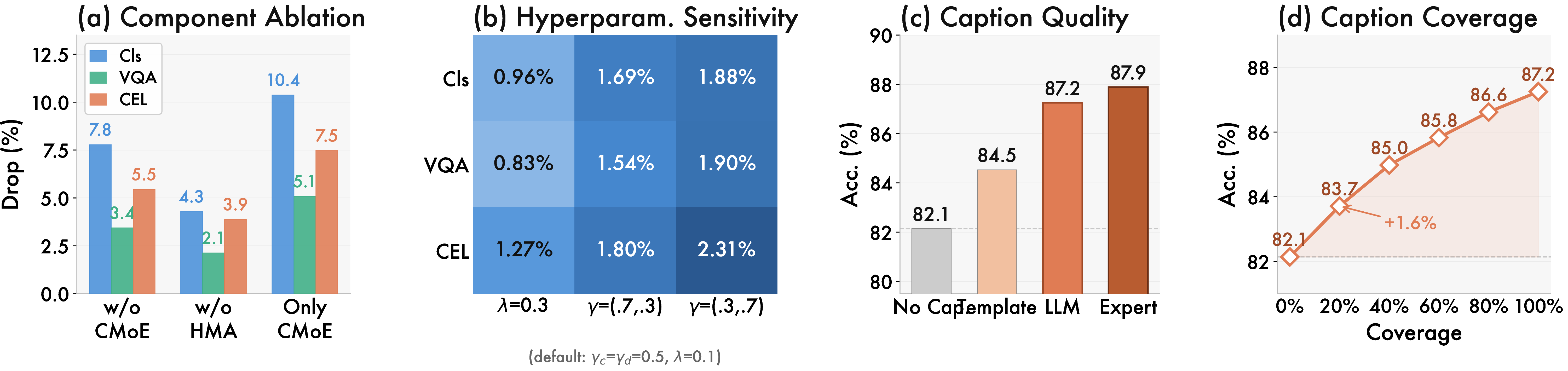
We analyze FM\(^2\) from six complementary angles: (i) component ablation (Fig. 3a), (ii) hyperparameter sensitivity (Fig. 3b), (iii) caption quality and coverage (Fig. 3c–d), (iv) communication cost (Table 7), (v) convergence behavior, and (vi) learned feature structure (Fig. 4). Unless noted, ablation and sensitivity results span three tasks: classification (MIMH-5-Domain, \(\varphi{=}0.1\), FM\(^2\)-Tiny), VQA (Task 1, F-CL, Non-IID), and CEL (MIMH-SA, FM\(^2\)+CEL), to verify that findings generalize across objectives.
4.4.0.1 Component Ablation.
We progressively disable FM\(^2\)’s core components (Fig. 3a). Among single-component removals, disabling CMoE costs 3.4–7.8% and disabling HMA costs 2.1–4.3%. The most harmful variant, Only CMoE, removes both DMoE and HMA and drops 5.1–10.4%, showing that personalization alone is insufficient without global domain consensus. Since w/o-HMA and Only-CMoE differ only in DMoE, removing DMoE alone still costs 5.4 and 1.8 points on MIMH-5-Domain and MIMH-SA, so DMoE contributes beyond a personalized CMoE plus the federated backbone. The importance ordering (Only CMoE \(>\) w/o CMoE \(>\) w/o HMA) is consistent across all three tasks, confirming architectural robustness independent of downstream objective.
4.4.0.2 Hyperparameter Sensitivity.
Fig. 3 (b) examines the effect of varying \(\gamma_c\), \(\gamma_d\), and \(\lambda\) away from the default setting (\(\gamma_c{=}0.5\), \(\gamma_d{=}0.5\), \(\lambda{=}0.1\)). Across all three tasks, no non-default configuration degrades performance by more than 2.31%, indicating that FM\(^2\) is not sensitive to precise hyperparameter tuning and that the default configuration generalizes reliably across diverse settings and tasks.
| Method | Comm. Params (K) | Comm./Rd (MB) | Time/Rd (s) | Acc. |
|---|---|---|---|---|
| FedAvg [14] | 520 | 41.6 | 8.2 | 23.05 |
| FedProx [37] | 520 | 41.6 | 9.5 | 38.70 |
| FedProto [43] | 1.3 | 0.1 | 7.8 | 70.84 |
| FedRep [19] | 450 | 36.0 | 9.1 | 74.72 |
| FM\(^2\)-Tiny | 718 | 57.4 | 12.5 | |
| FM\(^2\)-Medium | 824 | 65.9 | 14.8 | |
| FM\(^2\)-Large | 1035 | 82.8 | 18.3 |
4.4.0.3 Caption Quality and Coverage.
Fig. 3 (c–d) examines CEL robustness on MIMH-SA. LLM-generated captions (87.25%) nearly match expert annotations (87.89%) while far exceeding templates (84.53%), confirming API generation as a cost-effective substitute for manual labeling. Even at 20% coverage, CEL yields +1.57% over the image-only baseline, with monotonically increasing but diminishing returns, showing that CEL is beneficial even under the uneven caption availability typical of real federated deployments.
4.4.0.4 Communication Cost.
Table 7 reports per-round communication and wall-clock overhead. Because the CMoE module is entirely local (never communicated), the additional communication of FM\(^2\)-Tiny over FedAvg is 38% in parameter count (718K vs.520K), a modest price for a 60.75 percentage-point accuracy gain. FedProto achieves the lowest communication (prototype-only exchange) but plateaus at 70.84%. FM\(^2\)-Large uses \(2\times\) FedAvg’s bandwidth yet reaches 86.68%, representing a fundamentally different accuracy-communication trade-off.
4.4.0.5 Convergence and Feature Analysis.
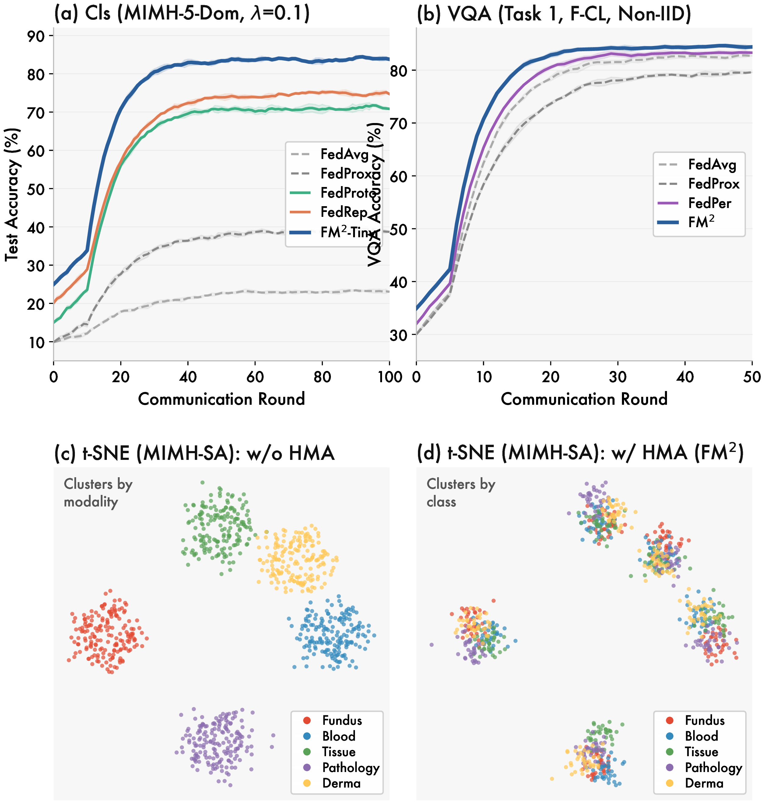
Figure 4 reports convergence and feature structure. On classification (Fig. 4a), FM\(^2\)-Tiny reaches 80% by round 40, a level no baseline achieves at round 100; FedAvg stagnates below 25% while FedProto and FedRep plateau near 70–75%. On VQA (Fig. 4b), FM\(^2\) converges fastest to 84.4%, above FedPer (83.3%) with tighter variance. t-SNE on MIMH-SA (Fig. 4c–d) shows that without HMA features cluster by modality; with HMA they reorganize by semantic class, with all five modalities interleaving within each cluster, validating HMA’s design objective and the out-of-modality generalization in Tables 1 and 3.
5 Conclusion↩︎
In this paper, we proposed FM\(^2\), a federated multimodal foundation model framework that addresses the under-explored challenge of Imaging Modality Heterogeneity in medical imaging. Through dual Mixture-of-Experts modules and Heterogeneous Modality Alignment with provable convergence guarantees, FM\(^2\) disentangles personalized class knowledge from shared domain representations. Extensions to Caption-Enhanced Learning and Federated Medical VQA demonstrate FM\(^2\)’s versatility as a multimodal foundation model. Extensive experiments on the MIMH benchmark (for classification and CEL) and real-world medical VQA datasets confirm consistent superiority over state-of-the-art baselines, fast convergence, strong out-of-modality generalization, and practical robustness to caption availability and hyperparameter choices.
This work was supported by the Guangdong Basic and Applied Basic Research Foundation (No. 2024A1515510031). This work is also supported by the Intelligent Computing Center of Shenzhen University.