A POS Tier Is the Key to Automated Annotation for Low-Resource Language Documentation: Neural Interlinear Glossing for Irabu, a Southern Ryukyuan Language
July 15, 2026
Abstract
Discourse data are the primary empirical basis of grammar writing in field linguistics, but producing interlinearized text is notoriously expensive — on the order of one hour of work per minute of recording. For endangered languages, where the time remaining to verify analyses with native speakers is itself limited, automating parts of the interlinearization workflow has direct documentary value. We implement a full neural annotation pipeline (morpheme segmentation \(\rightarrow\) POS tagging \(\rightarrow\) glossing) for Irabu Ryukyuan using deliberately small, transparent BiLSTM–CRF models, and evaluate it under a realistic hard constraint: approximately one hour of fully annotated discourse as the entire supervised resource. Two factors of the annotation itself are manipulated: its richness (with or without a POS tier) and its quantity (training budgets from 6 to 47 minutes). Gold POS improves grammatical glossing by \(+4.4\pm0.7\) points (significant in all 5 seeds), and the gain grows as data shrink (\(+11.6\) points at a quarter of the data); a POS tier more than halves the amount of glossed data needed to reach a given accuracy. In a fully automatic pipeline this gain is not yet realized: the tagger still errs on 12% of morphemes, and an incorrect POS misleads the glossing model more than no POS at all. The value is latent rather than lost: degrading gold POS with controlled noise shows the gain returning as tagger accuracy rises, with break-even near our tagger’s current 88% and \(+1.6\) to \(+3.2\) points recovered at 92–96%. We conclude with a concrete recommendation for documentation practice: annotate quadrilinearly — text, POS, gloss, translation.
Keywords: low-resource languages; language documentation; neural networks; automated glossing; Ryukyuan
1 Introduction↩︎
1.0.0.1 Background: the annotation bottleneck.
Documentary linguistics takes as its primary object a corpus of naturalistic communicative events — narratives, conversations, and whatever further event types the community’s culture-specific ways of speaking comprise: a “systematics” of communicative events [1]. For grammar writing, such connected discourse is an indispensable empirical resource: it supplies the frequency, context, and construction diversity that elicitation alone cannot [2], [3]. The cost side is equally well known: the gap between what is recorded and what is transcribed — the “transcription bottleneck” [4] — reflects, in our experience, on the order of one hour of expert work per minute of recording for fully interlinearized text ([2]; a similar guess is given by [4, p. e336]). In documentation projects for endangered languages, the Japonic–Ryukyuan languages among them, this annotation cost is the standing bottleneck between recording discourse and actually using it. For endangered languages the bottleneck is compounded by a harder limit: the time remaining with fluent speakers. Every hour spent mechanically filling in glosses is an hour not spent checking analyses with speakers. Research on automatic annotation is therefore not a convenience but a necessity for documentary linguistics, and the present study is squarely in that context: automation not as a replacement for the linguist, but as a way to reallocate scarce speaker-facing time.
1.0.0.2 Stance: leverage, not replacement.
The last point deserves emphasis, because it sets this study apart from much of the current, largely NLP-driven discussion of low-resource annotation automation, which tends — often implicitly — toward replacement: systems designed and benchmarked as if the goal were to produce interlinear text without the linguist in the loop. The tendency lives in the operational format rather than in stated aims: the SIGMORPHON glossing shared task, for instance, is prefaced by the remark that such methods “can never fully replace the expertise of a dedicated documentary linguist” [5] — yet what the task measures is precisely fully automatic production. For endangered-language documentation we consider that framing not just unrealistic but misdirected. Consider what a chef wants from automation: not to arrive at the restaurant and find every dish already cooked, but to be relieved of the shopping, the cleaning, and the slow, monotonous prep work — and to have even that done under the chef’s supervision, in a form the chef can inspect, because whatever leaves the kitchen carries the chef’s name. The documentary linguist is in the chef’s position. The discourse data being automated has a specific consumer: it exists to be used by descriptive linguists for grammar writing (as well as, of course, by language communities for revitalization purposes, which we do not go into in this study), and its annotations are meaningful only insofar as they conform to the gold analysis that the linguist’s own descriptive work produces — the label inventory, the segmentation conventions, the glossing decisions. Automatic output that drifts from that analysis is not a cheaper version of the same resource; it is a different resource of unclear value. The productive frame, we suggest, is the opposite of replacement: treat the small body of training data that a descriptive linguist can carefully hand-annotate in the time that remains as an asset, and ask how to leverage that asset for the maximum documentary return. The two questions below are the operational form of this view.
1.0.0.3 Problem: two questions without concrete answers.
Bringing automatic annotation into a documentation project immediately raises two practical questions. The first is model choice: what kind of model is appropriate under the data conditions of endangered-language documentation? The second — asked less often, but the one a project leader must answer first — is training cost: how much supervised data, of what kind, must the linguist create before automation pays off? That is, the minimum quantity and the minimum richness of the teaching annotation. For Japonic–Ryukyuan languages, concrete studies addressing either question are, to our knowledge, all but nonexistent [6]. The gap has consequences well beyond automation itself. Discourse-collection projects for endangered Japanese dialects are currently proliferating,1 yet how much discourse to record is typically set either as an open-ended aspiration (“as much as possible”) or by convention — one hour, two hours — with no empirical basis for the number; and how the collected discourse should be annotated receives even less attention: in many projects the recordings are transcribed and given a free translation only, with no morpheme-level annotation at all [8]. Without answers to the two questions above, there is in fact no principled way to set either the number of hours or the depth of annotation.
1.0.0.4 Purpose.
This study takes up both questions, in different ways matched to their nature. The first — model choice — we answer by design: small, transparent, purely supervised BiLSTM–CRF models, on grounds set out in the next paragraph. The second — training cost — is the empirical subject of the paper. We implement and evaluate a complete neural interlinearization pipeline — morpheme segmentation, POS tagging, and glossing — for Irabu, a Southern Ryukyuan language [9], [10], under a scenario we consider realistic for most endangered-language projects: the entire supervised resource — the asset to be leveraged — is about one hour of fully annotated discourse (774 utterance units, of which the 620-utterance training portion corresponds to roughly 47 minutes; §3), with sub-budgets down to 6 minutes evaluated explicitly (§3.7). The question is not “how well can neural models gloss with abundant data” but “what return does a given investment of annotation actually buy — and how should that investment be allocated?” Answering it yields what current practice lacks: an empirically grounded criterion — how many minutes of discourse to annotate, and with which tiers — in place of effort targets and conventional hour counts. Our budget-centered evaluation culminates in a concrete proposal: a two-stage design in which a small first-stage corpus is annotated richly, then leveraged to automate the rest (§6).
1.0.0.5 Model choice (the first question): small, supervised, and transparent.
All components are BiLSTM–CRF sequence labelers [11]–[13]. We deliberately do not use large pretrained Transformer models [14], [15], for two reasons. First, the data reality: the premise of unsupervised or transfer approaches — large amounts of raw text — does not hold for most endangered languages, where the recorded discourse itself is minuscule; under such conditions we consider it more realistic to invest the linguist’s expertise in careful annotation of the small data and use it as direct supervision. We have previously framed this as a quality-dependent rather than quantity-dependent scenario [6]: an experienced fieldworker can produce a small but highly consistent gold-standard corpus, which is precisely the setting where small supervised models are viable. Second, workflow transparency: a BiLSTM–CRF factorizes into per-morpheme evidence (emission scores) and label-sequence regularities (transition scores), a structure that maps naturally onto how a linguist reasons about interlinear annotation, and whose errors are correspondingly diagnosable (§3.5 puts this transparency to work). We emphasize the scope of this choice: we make no claim that small supervised models outperform pretrained ones — indeed, pretrained multilingual encoders can be viable even for low-resource languages [16], [17], although “low-resource” there still means raw text on the gigabyte scale or sizable monolingual corpora (AfriBERTa pretrains on just under 1 GB; the transcription tier of our corpus totals \(\sim\)26 KB, four orders of magnitude less) — and comparing against such encoders and LLM-based approaches [15], [18], [19] under the same annotation budget is future work. Our contribution concerns annotation design under a fixed, simple model.
1.0.0.6 Terminology: trilinear vs.quadrilinear.
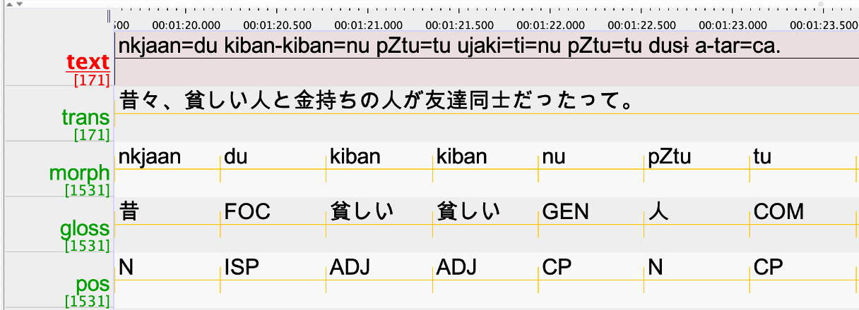
Standard IGT is trilinear: a transcription line, a morpheme-by-morpheme gloss line [20], and a free-translation line. Note where the annotator’s morpheme-level effort goes: it is concentrated entirely in the gloss line. A parallel morpheme-by-morpheme POS tier is not part of common practice — part-of-speech information remains implicit in the analysis, or is recorded only in the lexicon, but is rarely written down token by token. We use quadrilinear for the format that adds exactly this tier (text + POS + gloss + translation); Figure 1 shows the resulting tier structure in our ELAN workflow. Two clarifications are important. First, the POS tier at issue is per morpheme, aligned with the gloss line, not a per-word category label. Second, while the free-translation line is part of both formats, our system does not use it at any stage: unlike translation-leveraging approaches to glossing [21], [22], our pipeline operates entirely on the transcription, POS, and gloss tiers. Figure 1 shows what quadrilinear annotation looks like in practice, in the ELAN environment in which our corpus was built. What our experiments quantify, therefore, is the return on deliberately annotating the one morpheme-level tier that standard practice omits.
1.0.0.7 What we test.
Holding the model fixed, we manipulate the annotation itself along two axes:
Richness (RQ1): does the POS tier — quadrilinear rather than trilinear annotation — improve automatic glossing? We separate the intrinsic value of POS information (oracle input) from its realizable value in a full pipeline (predicted input), and dissect the gap token by token.
Quantity (RQ2): how does performance scale from 6 to 47 minutes of annotated discourse, and does it interact with richness?
1.0.0.8 Contributions.
(i) A complete, reproducible neural interlinearization pipeline for a low-resource Ryukyuan language,2 trained on \(\sim\)47 minutes of annotated discourse, with budgets down to 6 minutes evaluated (segmentation span-F1 0.907; POS accuracy 0.881; grammatical-gloss accuracy 0.93 with oracle POS). (ii) A controlled ablation showing that POS information improves grammatical glossing by \(+4.4\pm0.7\) points (all 5 seeds individually significant), with the gain concentrated on linguistically predictable ambiguities (case/focus clitics). (iii) An error-propagation analysis showing that with a realistic tagger the gain is cancelled — incorrect POS is worse than no POS — and an exact decomposition of the loss, plus a noise-injection analysis locating the break-even tagger accuracy (\(\approx\)88%). (iv) A data-size analysis showing the POS gain grows as data shrink (up to \(+11.6\) points at \(\sim\)12 minutes), so a POS tier more than halves the glossed data needed — exactly in the regime where documentation projects begin. (v) A concrete recommendation for annotation practice: quadrilinear annotation, with quantified costs and benefits — and, building on it, a two-stage design for discourse-documentation projects (collect \(\sim\)30 minutes and annotate it richly first; then collect more and let the pipeline draft the annotations). (vi) A working implementation of the Stage-2 workflow: a browser-based annotation tool in which the pipeline drafts the interlinearization of arbitrary input, the annotator confirms or corrects every tier, and the corrections feed back into the models (Figure 8).
2 Related Work↩︎
2.0.0.1 Automatic interlinear glossing.
Automating IGT production has a substantial NLP literature. [23] evaluated machine-in-the-loop annotation strategies for documentation; [24] showed that CRF-based glossing reaches useful accuracy for Lezgi from roughly 3,000 words of IGT — a setting close to ours in scale and spirit, down to the design decision of reducing open-class stems to a placeholder and predicting the closed-class grammatical glosses — and [25] report a comparable case study for Otomi. Notably, Moeller and Hulden’s models consume a POS tier rather than evaluate it: word-level POS tags enter their CRF as features (“and, of course, POS tags taken from the data,” [24, p. 88]), on the explicit assumption that documentation data will come with POS. Their POS-informed CRF outperforms their no-POS seq2seq by 13 points, but the two differ in architecture, so the tier’s own contribution cannot be isolated; our ablation turns exactly this assumed ingredient into a measured design variable. (Suggestively, their hardest labels are case morphemes such as gen and erg — precisely where our POS gain concentrates; Appendix 8.) Later work leverages the translation line [21], [22], [26]: [26] generates the gloss line from the segmented source phrase plus its English translation, [21] feed translations to a multi-source transformer, and [22] quantify the tier’s effect: embedding LLM-encoded translations into a hard-attentional glosser gains \(+4.0\) points on average over the previous state of the art on the SIGMORPHON 2023 data, and \(+9.8\) points over the translation-free baseline when training on as few as 100 sentences — the same band as our POS-tier gain (\(+4.4\) with full data, \(+11.6\) in the low-data regime), for a tier that trilinear practice already produces. A POS tier, by contrast, is far cheaper than free translation (a closed inventory) yet is the tier standard practice does not write down. This strand culminated in the SIGMORPHON 2023 shared task on interlinear glossing [5] and its systems [27]. Most recently, massively multilingual pretraining [15] and LLM-based glossing [18], [28] have been explored — the latter with an interactive, linguist-assisting orientation close in spirit to ours [18] — and [19] probe gloss prediction as one test of what LLMs learn about a low-resource language from a grammar book. This line of work asks “how accurate can glossing get given a corpus”; our question is the converse and, to our knowledge, largely unaddressed: given a fixed, small annotation budget, how should the annotation itself be designed — which tiers, how much? Our controlled comparison of annotation richness (POS tier) and quantity, with seed-level significance testing and error-propagation analysis, is complementary to all of the above.
2.0.0.2 Ryukyuan and Japanese dialects.
To our knowledge, the only prior work on IGT automation for Japonic varieties is our own proof-of-concept for Irabu [6], which introduced the quality-dependent scenario, a joint segmentation–POS–gloss prototype, and a dictionary on/off comparison, but no controlled ablation, no multi-seed significance testing, and no analysis of error propagation or annotation budgets. Trained on a 30-minute subset of the present corpus (289 sentences), that system reached 97.2% word-level segmentation exact match, 84.7% gloss-token accuracy (dictionary-assisted, lexical and grammatical glosses pooled), and 75.4% POS accuracy on a 30-sentence held-out set. The numbers are not directly comparable to ours — the data volume, test sets, metrics, and task decomposition all differ — but the qualitative picture is consistent: under the present paper’s stricter evaluation (405 grammatical-gloss tokens, five seeds), the redesigned pipeline improves POS tagging (0.75 \(\rightarrow\) 0.88) and reaches 0.89–0.93 on grammatical glosses, superseding the prototype on all fronts. Beyond IGT, NLP interest in endangered Japonic varieties is now emerging on the translation side: [29] machine-translates the Yoron dialect (Amami Islands) into Japanese with retrieval-augmented LLM generation over roughly 9,000 phrase-aligned pairs drawn from a published folk-tale collection. That line exploits the phrase-translated (non-IGT) resources that Japanese dialectology has produced in relative abundance, and large proprietary LLMs; ours targets the annotation tiers that only IGT provides — segmentation, POS, and gloss — with small supervised models. The two are complementary halves of the same documentary bottleneck.
2.0.0.3 The documentation bottleneck.
The programme of documentary linguistics — compiling annotated corpora of primary data for endangered languages — was articulated by [1]; [4] review its first twenty-five years and identify the transcription bottleneck as a central obstacle. On the audio side of that bottleneck, [30] integrated automatic transcription into the Na documentation workflow; our work addresses the complementary annotation side (segmentation, POS, gloss), and the two lines compose naturally into a single pipeline. CRF-based morphological segmentation in low-resource settings was established by [31]. In Japan the bottleneck is also institutional: [7] surveys ongoing collaborative efforts to digitize, align, and native-check legacy dialect recordings — most notably the 1977–1985 national emergency survey (roughly ten hours of discourse at each of 228 sites) — four decades after their collection; we return to this in §6.
3 Data and Pipeline↩︎
3.1 Corpus↩︎
Our corpus consists of 774 transcribed utterance units of Irabu Ryukyuan (6,412 morpheme tokens), drawn from four recordings totalling 58 minutes 26 seconds of connected discourse. The materials are entirely original fieldwork by the author, recorded
with five speakers of the Nagahama district of Irabu island between 2005 and 2025; the genres are monologue — mostly legends and folktales — and everyday conversation. Transcription and annotation were likewise carried out by the author: the corpus is
fully annotated with morpheme boundaries, POS tags (32 tags, of which 31 occur in the training split; full inventory in Appendix 7), and interlinear morphemic glosses [20]; annotation was carried out in ELAN following the workflow described in [6],
whose corpus (roughly 30 minutes) forms a subset of the present one. The corpus also carries a free-translation tier, but — as stated in §1 — no component of the pipeline uses it; all supervision comes from the
transcription, POS, and gloss tiers. We distinguish grammatical glosses (a closed set of category labels such as nom, gen, foc; 115 types in training)
from lexical glosses (open-class Japanese translations). This paper’s quantitative target is the former; lexical positions are mapped to a placeholder lex so sentence context is preserved. Data are split at utterance
level into train/dev/test (620/77/77 utterances; Table 1). The gold corpus (final.json), all pipeline and experiment code, and the complete per-sentence test outputs (test_report.txt) are available in
the repository cited in §1 (https://github.com/MichinoriShimoji/ML_autogloss).
| Split | Utt. | Tokens | Gram.tok. | Label types |
|---|---|---|---|---|
| Train | 620 | 5,075 | 3,145 | 115 |
| Dev | 77 | 675 | 432 | 76 |
| Test | 77 | 662 | 405 | 64 |
3.2 Pipeline Components↩︎
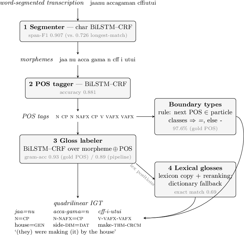
The pipeline (Figure 2) mirrors the interlinearization workflow: (1) a character-level BiLSTM–CRF segments words into morphemes (test span-F1 0.907, vs. for a longest-match dictionary baseline; \(p<10^{-4}\), paired randomization/bootstrap); (2) a BiLSTM–CRF POS tagger over morphemes (test accuracy 0.881); (3) the glossing model described next. A lexical-gloss module (training-lexicon copy with contextual reranking plus a fallback to a digitized dictionary of a neighboring variety, [32]) reaches 0.69 exact match but is peripheral here.3
3.2.0.1 Boundary types come from POS.
IGT distinguishes affixal boundaries (-) from clitic boundaries (=), so a segmenter must in principle deliver typed boundaries. Our design factors this apart: the segmenter predicts boundary positions only, and the type is derived from the POS of the following morpheme — particle classes (case, focus, final, conjunctive, etc.) attach with =, affix classes with -. In our corpus this majority rule reconstructs the type of 97.6% of all 3,613 word-internal boundaries (and, fit on the training split alone, scores 97.8% on the 368 held-out test boundaries): the affix/clitic distinction is, to a close approximation, a corollary of lexical category. The alternative — a segmenter trained to predict typed boundaries jointly (eight labels instead of four) — is empirically just as good at segmenting: across 5 seeds, position span-F1 is \(0.901\pm0.013\) (typed) versus \(0.900\pm0.009\) (plain), and type accuracy at correctly detected positions averages 97.8%.4 Which route should deliver the type therefore depends on the quality of the POS the rule consumes, and we measured both (test set, 368 boundaries; experiment released with our code). On gold POS the rule ties the typed segmenter (97.8%). On predicted POS it falls to 95.4% — whether segmentation is gold or predicted — while the typed segmenter, which never consults POS, keeps \(97.8\pm0.4\)% at the positions it detects: a \(+2.4\)-point advantage, consistent in direction in all 5 seeds (pooled discordant boundaries 60:17; exact McNemar significant in 2 of 5 seeds). For a fully automatic pipeline, then, typed segmentation is the better engineering choice. Our deployed interactive tool still derives types from POS, for a workflow reason: keeping one source of truth means a POS correction automatically corrects the attached boundary type, and once the annotator has reviewed the POS tier — which the Stage-2 workflow requires anyway — the rule operates on gold-quality tags and recovers its 97.8% ceiling. This is a first instance of the paper’s recurring theme — the POS tier quietly carries other tiers of IGT with it — and, in the same breath, of its qualification: it carries them at gold quality, and tagger errors tax the ride (§3.5 quantifies the same pattern for glossing).
We ask whether a POS tier — quadrilinear rather than trilinear annotation — improves automatic grammatical glossing. We separate two questions: (A) does POS information have intrinsic value for gloss prediction, and (B) can that value be realized in a fully automatic pipeline, where POS tags themselves must be predicted?
3.3 Glossing Model and Conditions↩︎
The glossing model is a BiLSTM–CRF over morphemes: each morpheme is represented by a 64-dimensional embedding, optionally concatenated with a 16-dimensional POS embedding, fed to a single-layer BiLSTM (hidden size 128) with a CRF output layer. Note where each information source acts: POS is visible only to the BiLSTM, as an input feature; the CRF operates purely over the output gloss labels, scoring adjacent label pairs, and never sees POS. All other factors — data splits, architecture, optimizer (Adam, lr \(10^{-3}\)), batch size (16), training length (40 epochs, best-dev selection) — are held constant; the only manipulated factor is the POS input. Three conditions:
Gold POS (oracle): human POS tags at training and test time. Measures the intrinsic value of POS (question A). Not available in deployment, but operative in computer-assisted annotation, where a human supplies POS before the model proposes glosses.
Predicted POS (pipeline): test-time tags from the POS tagger of §3 (accuracy 0.881). Measures realizable value (question B), including error propagation. The information flow is identical to the Gold-POS condition: the tagger first Viterbi-decodes the complete POS sequence for the sentence, and the glossing model then receives those tags exactly as it would receive gold ones — the two conditions differ in input quality, not in architecture; nothing is predicted jointly.
No POS (control): the POS embedding is ablated.
Both models are trained from scratch with five random seeds (mean \(\pm\) SD reported). Within each seed, Gold-POS and No-POS systems are compared on the same 405 test tokens with an exact McNemar test.
3.4 Main Results (RQ1: Richness)↩︎
![Figure 3: How the trained model glosses ga in example ([ex:gen]),with actually measured scores. POS participates only as an input feature:the BiLSTM merges the flanking nouns’ categories into ga’s contextualvector, and the resulting emission already ranks gen abovenom (+9.5 vs.+8.6; the emission-only argmax is alreadygen). The CRF sees no POS; it scores adjacent gloss labels, yetits learned transitions also favor gen here (net +0.4) —syntax echoed in label-sequence statistics. Contribution to the decision:roughly 2/3 emission, 1/3 transitions.](/article/2607.13372/_pdflatex/ebkrvymw.png "fig:")
| Condition | Gram.gloss accuracy |
|---|---|
| Gold POS | 0.937 \(\pm\) 0.004 |
| Predicted POS | 0.897 \(\pm\) 0.006 |
| No POS | 0.893 \(\pm\) 0.008 |
| \(\Delta\)(Gold \(-\) No) | \(+4.35 \pm 0.73\) pts |
| \(\Delta\)(Predicted \(-\) No) | \(+0.40 \pm 0.77\) pts |
| Seed | Gold | Pred. | No POS | \(\Delta\)(Gold\(-\)No) | McNemar \(p\) |
|---|---|---|---|---|---|
| 1 | 0.936 | 0.891 | 0.889 | \(+4.7\) | \(1.6\times10^{-4}\) |
| 2 | 0.943 | 0.904 | 0.901 | \(+4.2\) | \(7.6\times10^{-5}\) |
| 3 | 0.933 | 0.894 | 0.882 | \(+5.2\) | \(1.9\times10^{-5}\) |
| 4 | 0.933 | 0.894 | 0.901 | \(+3.2\) | \(7.2\times10^{-3}\) |
| 5 | 0.938 | 0.904 | 0.894 | \(+4.4\) | \(2.8\times10^{-4}\) |
With gold POS, the POS-informed model outperforms the ablated model by \(+4.35\pm0.73\) points; the gain is positive and individually significant in all five seeds (Tables 2–3; all \(p<0.01\), hence significant even under Bonferroni correction for the five tests). POS information is intrinsically valuable for grammatical glossing (question A: yes).
3.4.0.1 Why POS helps: the case of ga.
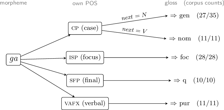
The Irabu clitic ga occurs 112 times in our corpus under six distinct grammatical glosses, and its segmental form gives no clue. Yet with POS in hand, the ambiguity dissolves into rules a linguist would state on one line (all counts are corpus totals):
If ga is a case particle (cp), the next word decides: \(N\) =ga \(N\) \(\rightarrow\) gen (‘X’s Y’; 27/35), whereas \(N\) =ga \(V\) \(\rightarrow\) nom (subject; 11/11).
If ga’s own POS is isp, the gloss is forced: focus particle ga is foc without exception (28/28). Likewise sfp \(\rightarrow\) q (10/10) and vafx \(\rightarrow\) pur (11/11).
Figure 4 schematizes this disambiguation, and ([ex:gen])–([ex:foc]) are real corpus utterances instantiating it: in ([ex:gen]) ga sits between two nouns (gen), in ([ex:nom]) a verb follows (nom), and in ([ex:foc]) ga itself is a focus particle (isp), which forces foc. Note that ([ex:nom]) and ([ex:foc]) are string-wise near-parallel (…=ga …-tar=gagara=mmja); only the POS tier tells them apart.
otoo =ga fni =nu =du f =ti
n cp n cp isp v cjp
father gen boat nom foc come quot
‘(They said) father’s boat is coming.’ taa =ga tur -tar =gagara =mmja
prn cp v vafx mp intj
who nom take pst dub dsc
‘Who took it, I wonder.’ unu nausi =ga maf -tar =gagara =mmja
intj adv isp v vafx mp intj
fil how foc wind pst dub dsc
‘How did it wind up, I wonder.’
These category-level rules are exactly what the POS-informed model can exploit and what a morpheme-only model cannot see: on the test set, the ablated model misglossed ga as nom in both ([ex:gen]) and ([ex:foc]) — the actual errors we observed — and resolved only 7 of 10 grammatical ga tokens overall, versus 10/10 with POS.5 Appendix 8 confirms the pattern corpus-wide: the largest per-label gains fall exactly on the case and focus/topic clitics (Table 8).
3.4.0.2 Where in the model the rule lives.
It is worth being precise about where the \(N\) =ga \(N\) rule is computed, because the answer illustrates the transparency we appealed to in §1. Figure 3 traces example ([ex:gen]) through the trained model, with actually measured scores. POS enters at the very bottom, as an input embedding concatenated to each morpheme embedding. The BiLSTM then folds the left context (otoo, n) and the right context (fni, n) into ga’s contextual vector, and a linear layer converts that vector into emission scores — one score per gloss label. The categorical rule is already decided at this point: gen scores \(+9.5\) against nom’s \(+8.6\), so even before the CRF, the emission argmax is gen. The CRF, which never sees POS, then adds transition scores between adjacent output labels and Viterbi-decodes the globally best gloss sequence. Interestingly, its transitions push in the same direction (net \(+0.4\)), and the reason is instructive. At the label level the two competitors look identical here — lex gen lex vs.lex nom lex — so one might expect the CRF to be indifferent. It is not, because the two labels have sharply different continuation profiles in the training data: gen, being adnominal, is followed by a lexical gloss 95% of the time (118/124), whereas nom is followed by a lexical gloss only 64% of the time (43/67), with much of the remaining mass on foc (18%) — reflecting the Miyako focus construction in which a nominative subject hosts the focus clitic =du, visible in example ([ex:gen]) itself (fni=nu=du). The learned transitions mirror this exactly: gen\(\rightarrow\)lex (\(+0.23\)) is gen’s highest-scoring continuation, while nom’s is nom\(\rightarrow\)foc (\(+0.20\)), leaving nom\(\rightarrow\)lex at \(-0.10\). In a lex _ lex frame, then, the CRF favors gen not because it sees the syntax, but because nom’s expected continuation (foc) fails to appear — a distributional echo of the syntax in the label space, learned without ever seeing a POS tag. The decision thus decomposes into interpretable parts: roughly two thirds context-driven emission (the POS-informed BiLSTM) and one third label-sequence prior (the CRF).
With predicted POS the gain shrinks to \(+0.40\pm0.77\) points — smaller than its seed variance, one seed negative, and non-significant by an exact McNemar test in every seed (smallest \(p=0.44\)). The current pipeline does not realize the value of POS (question B: not yet). §3.5 locates the loss.
3.5 Analysis: Where the 4 Points Are Lost↩︎
| Gloss accuracy at these positions | |||
|---|---|---|---|
| 2-4 Position type | Gold POS | Predicted POS | No POS |
| Tagger correct (371 tok., 91.6%) | 0.963 | 0.960 | 0.930 |
| Tagger error (34 tok., 8.4%) | 0.653 | 0.218 | 0.494 |
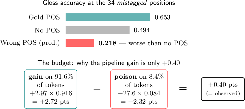
Gold and predicted POS differ only where the tagger errs, so the 4-point gap must originate there (the released test report shows the propagation sentence by sentence). To see how, we split the 405 test tokens into two groups — the 371 (91.6%) where the tagger predicted the token’s own POS correctly, and the 34 (8.4%) where it did not — and ask how each model fares in each group (Table 4, visualized in Figure 5). Three findings follow.
3.5.0.1 (a) The damage is localized.
Where the tagger is right, nothing is lost: the POS-informed model performs as well with predicted POS as with gold (0.960 vs.). Essentially all of the damage sits in the small mistagged group: there, switching from gold to predicted POS flips 44.1% of the glosses from correct to incorrect, against a negligible 0.4% elsewhere.
3.5.0.2 (b) At those positions, a wrong POS is worse than no POS.
This is the key finding (Figure 5, top). One might expect a wrong POS to be merely useless. It is not: at mistagged positions the model that receives the (wrong) POS scores 0.218, far below the 0.494 of the model that receives no POS at all. A wrong tag is misleading evidence — the model, trained exclusively on gold POS, has never seen an incorrect tag and follows it off a cliff (a train/test mismatch akin to exposure bias).
3.5.0.3 (c) The two effects balance almost exactly.
The observed pipeline gain is now just bookkeeping (Figure 5, bottom): on the 91.6% of well-tagged tokens, POS earns \(3.0\) points per token (\(0.9596\) vs.\(0.9299\)); on the 8.4% of mistagged tokens it loses \(27.6\) points per token (\(0.2176\) vs.\(0.4941\)). Weighting by group size, \[\begin{align} &\underbrace{(0.9596-0.9299)\times0.916}_{+2.72\;\text{pts (gain)}} + \underbrace{(0.2176-0.4941)\times0.084}_{-2.32\;\text{pts (poison)}}\\ &\qquad = +0.40\;\text{pts}, \end{align} \label{eq:budget}\tag{1}\] which reproduces the observed \(+0.40\) exactly. In words: each tagger error is roughly nine times as damaging as each correct tag is helpful, so 8% poison cancels 92% gain. The pipeline gain vanishes not because POS lacks value, but because of where and how the errors strike.
3.6 Break-Even Analysis: How Good Must the Tagger Be?↩︎
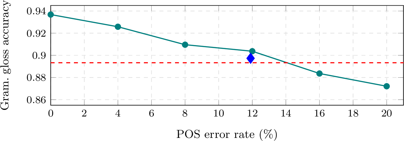
Injecting controlled noise into gold POS — substitution errors sampled from the real tagger’s confusion distribution — traces how tagger quality translates into gloss quality (Figure 6). The POS-informed model beats the baseline by \(+3.2\) points at a 4% error rate and \(+1.6\) points at 8%, crossing it at 14.1%. Two caveats sharpen the picture. First, the real tagger (11.9% error) yields only \(+0.40\), below the simulated curve at the same rate: real errors cluster on hard tokens, so the effective break-even for a real tagger is nearer 88% accuracy — almost exactly where our tagger stands (88.1%). Second, the curve sets a concrete target: a tagger at 92–96% accuracy converts the latent value into \(+1.6\) to \(+3.2\) practical points.
3.7 Interaction with Data Size (RQ2): POS as a Data Multiplier↩︎
If POS acts as a coarse generalization class, its value should be greatest when training data are scarce — the situation at the start of a documentation project. We train both conditions on nested subsets of the training data (78, 155, 310, 620 utterances \(\approx\) 6, 12, 23, 47 minutes of discourse), rebuilding all vocabularies from each subset; five seeds per cell, gold POS at test.
| Train.utt. | \(\approx\)min | Gold POS | No POS | \(\Delta\) (pts) |
|---|---|---|---|---|
| 78 | 6 | 0.765 | 0.671 | \(+9.5\) |
| 155 | 12 | 0.839 | 0.723 | \(+11.6\) |
| 310 | 23 | 0.890 | 0.822 | \(+6.8\) |
| 620 | 47 | 0.933 | 0.888 | \(+4.5\) |
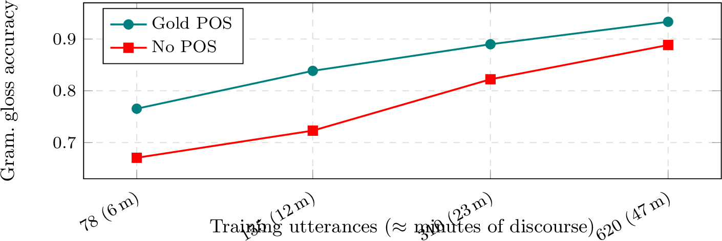
The interaction is substantial (Table 5, Figure 7): the gain peaks at \(+11.6\) points with a quarter of the data and shrinks to \(+4.5\) with all of it — a narrowing of \(2.0\) points per doubling of training data (seed-level regression, interaction \(t=-5.0\); analysis released with our code). At the smallest budget the gain is somewhat smaller (\(+9.5\) at 6 minutes than \(+11.6\) at 12), suggesting a floor below which the glossing model has too little data to exploit the tier fully. One qualification is important, because the two curves in Figure 7 nevertheless run roughly parallel to the eye — and on the log-odds scale they are parallel: there the interaction vanishes (\(t=0.5\)), and POS multiplies the odds of a correct gloss by a factor that stays within 1.6–2.0 (mean \(\approx\)1.8) at every budget. The two readings are complementary, not contradictory. POS confers a roughly constant multiplicative advantage; near the accuracy ceiling that constant multiplier compresses into a few percentage points, while in the low-data regime it unfolds into many. What an annotator experiences, however, is percentage points — glosses to fix per hundred — so the practical return on the POS tier is largest exactly where documentation projects begin. The same fact can also be read scale-free, as data equivalence: matching the POS-informed model trained on 78 utterances takes the ablated model \(\sim\)221 utterances (\(\times2.8\)); at 155, \(\sim\)386 (\(\times2.5\)); and the POS-informed model trained on half the corpus is not matched by the ablated model even with the full corpus. In this range a POS tier more than halves the glossed data needed for a given accuracy. (These curves use gold POS and thus speak to the assisted-annotation scenario; a pipeline analogue would retrain the tagger at each size — future work.)
4 Implications for Annotation Practice↩︎
Our results support a concrete recommendation for endangered-language documentation: include a POS tier — annotate quadrilinearly. The argument has three layers, in decreasing order of immediacy.

Computer-assisted annotation (immediate). In an interactive workflow where the annotator confirms or corrects POS before the model proposes glosses, the model effectively receives gold POS and the full \(+4.35\)-point gain applies. Figure 9 makes the order of operations explicit, because it is easy to misread: the pipeline drafts every tier at once, but the gloss line of that first draft is a preview, computed from unverified POS — it is never the object of correction. The annotator verifies the POS line (boundaries follow automatically); the glosses are then re-predicted from the verified tags — a millisecond re-decode in our tool — and only these proposals, now operating under the Gold-POS condition of Table 2, go to gloss review. POS is a small closed set (32 tags) and far cheaper to annotate than glosses; a cheap tier accelerates the expensive one. Note the cost asymmetry at the moment of annotation: for an annotator who has just segmented a morpheme and chosen its gloss, its part of speech is typically already decided in the analysis — recording it is nearly free. Conventional practice leaves this tier unwritten; our results show that the return on writing it down is large. The data-size analysis (§3.7) sharpens this: the gain is largest precisely when the corpus is small — at the start of a documentation project — where a POS tier more than halves the glossed data needed. The POS tier also subsumes another piece of IGT for free: the affix/clitic boundary typing (- vs.=) is recoverable from gold POS at 97.6% (§3.2), so annotating POS effectively annotates boundary types as well.
Fully automatic glossing (as annotation accumulates). The break-even analysis shows the pipeline gain is a function of tagger accuracy, which grows with annotated data. Quadrilinear annotation is thus an investment: once the tagger clears roughly 90%, POS begins to pay off automatically, approaching the \(+4.35\)-point ceiling.
Model-side remedies (future work). The poisoning effect (Table 4) suggests training with predicted or noised POS (scheduled sampling / POS dropout), joint POS–gloss modeling, or soft (probabilistic) POS inputs — each attacks the \(-2.32\)-point term of Eq. 1 rather than the tagger itself.
We emphasize what our data do not show: with the current corpus size, quadrilinear annotation does not yet improve fully automatic glossing significantly (\(+0.40\pm0.77\)). The recommendation rests on the assisted workflow, the measured ceiling, and the quantified path between them.
5 Limitations↩︎
Our conclusions are bounded in five ways. First, everything rests on a single language and a single corpus — roughly one hour of discourse, with a test set of 405 grammatical tokens; the numbers should be read as one carefully measured data point, not as universal constants. Second, the learning curves that ground the richness-beats-quantity argument use gold POS at test time, so they speak directly to the computer-assisted scenario and only indirectly to the fully automatic pipeline, whose tagger would itself improve as data grow. Third, we compare annotation designs under one deliberately simple, fixed model family; we have not benchmarked multilingual pretrained encoders or LLM-based glossing under the same annotation budget, so our claims rank annotation strategies, not model families. Fourth, lexical glossing — the open-class translation tier — is treated only peripherally, by lexicon copy with reranking. Finally, the two-stage sizing proposal (§6) extrapolates from one language’s learning curves, and its Stage-2 savings are a projection: the correction rate is measured, but the wall-clock review time in a live project is not yet.
6 Conclusion: A Two-Stage Design for Discourse Documentation↩︎
Discourse-collection projects for endangered languages routinely face a sizing decision — how much discourse to record, transcribe, and annotate — and, in our experience, that decision is usually made by convention (“one hour,” “two hours”) rather than by evidence about what a given amount of annotation buys. Our budget-centered results turn this into an empirical question, and they suggest a concrete answer for projects comparable to ours.
6.0.0.1 The proposal.
Structure the project in two stages:
Stage 1 — small, rich, careful. Collect roughly 30 minutes of discourse and invest the annotation effort there: full interlinearization in quadrilinear format (text + POS + gloss + translation), verified with speakers. Our results quantify what this buys: at a \(\sim\)23-minute training budget the POS-informed glossing model already reaches 0.89 (assisted), and with our full \(\sim\)47-minute corpus the pipeline reaches segmentation span-F1 0.91, POS accuracy 0.88, and grammatical-gloss accuracy 0.93 when a human supplies POS (0.89–0.90 fully automatically).
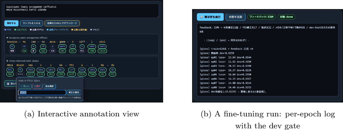
Stage 2 — collect more, correct instead of create. For all subsequent recordings, let the Stage-1 pipeline draft the interlinearization, and shift human effort from creating annotations to reviewing them, in an interactive workflow where each correction feeds back into the models and the speaker-facing time is spent on verification, not mechanics. We have built a working implementation of this workflow (Figure 8): a browser-based tool in which the pipeline annotates arbitrary input, every tier (including morpheme boundaries) can be confirmed or corrected in place, lexical-gloss corrections take effect immediately through a user lexicon, and accumulated corrections periodically fine-tune the three models (oversampled relative to the base corpus). Two design points matter for scientific hygiene: corrections whose sentences coincide with the held-out sets are automatically excluded from fine-tuning, so evaluation stays uncontaminated; and the deployed models are versioned separately from the frozen ones behind this paper’s numbers. The notorious 60:1 transcription bottleneck becomes, for the annotation tiers, a review task — and the review load is measurable: run end-to-end on our held-out test set, the pipeline delivers 63.6% of word tokens fully correct across all tiers (187/294; 24 of the 77 utterances need no edit at all), so the reviewer edits roughly one word in three instead of authoring four tiers for every word. Each reviewed hour, moreover, is not just annotated discourse but new training data: folded back into the gold corpus as a versioned revision (with the hygiene above applied), it moves the models along the learning curves of §3.7 — and once the tagger clears the break-even of §3.6, the currently latent POS gain compounds the improvement. Review effort per hour of discourse thus falls as the archive grows, though not to zero: the curves flatten, and reviewed output must be audited before promotion to gold, lest model errors be ratified into the record. How the correction rate converts into wall-clock savings is the Stage-2 measurement we call for below.
6.0.0.2 Why 30 rich minutes rather than an hour of plain ones.
The richness–quantity interaction (§3.7) directly informs how a fixed annotation budget should be split: a POS-informed model trained on half our corpus (\(\sim\)23 minutes) already matches an ablated model trained on all of it (\(\sim\)47 minutes; 0.890 vs.) — rich half-hour-scale annotation buys what plain hour-scale annotation buys. Since the POS tier adds only a small fraction of the per-utterance cost — a closed inventory of 32 tags, versus open-ended glossing and translation — richly annotating less discourse is the better investment than thinly annotating more. In the low-data regime where every documentation project begins, annotation richness beats quantity.
6.0.0.3 A concrete horizon: legacy discourse archives.
The scale of the opportunity in Japan alone is illustrated by the Agency for Cultural Affairs’ emergency dialect survey (1977–1985), which recorded roughly ten hours of discourse at each of 228 sites nationwide. Four decades later, making those recordings research-ready — digitization, alignment, native checking — is still ongoing, sustained by collaborative projects that recruit volunteer researchers and distribute the manual labor [7]. Legacy archives of this kind are precisely where the two-stage design points: for any variety in the archive that a researcher commands, a Stage-1 investment of some thirty richly annotated minutes would let a pipeline draft the remaining hours for review rather than creation. The current curation efforts target transcription and phrase-level translation rather than IGT; our proposal complements them by showing how such archives could be lifted to the IGT standard at realistic cost — and the two efforts could share infrastructure, since curated, aligned transcripts are exactly the input our pipeline expects.
6.0.0.4 Outlook.
The specific figure of 30 minutes is derived from one language and one corpus; the two-stage logic, however, only requires that the learning curves retain their shape — steep early gains, richness amplifying them — which we expect to be robust for agglutinative languages with comparable morphological transparency. Replicating the budget analysis across languages, closing the gap between oracle and pipeline POS (via better taggers or POS-robust training), and measuring the actual review-time savings in Stage 2 are the natural next steps.
7 POS Tag Inventory↩︎
Table 6 lists the complete POS tag inventory with corpus frequencies. Tag names follow the annotation scheme of the Irabu reference grammar [10]. The inventory has a long tail: five tags occur exactly once in the corpus, and onm occurs only outside the training split — the source of the unseen-label errors visible in Table 7.
3.5pt
8 Per-Label Performance↩︎
Table 7 breaks the POS tagger’s test performance down by tag, under exactly the condition behind the headline number of §3.2 (sentence-by-sentence decoding; overall accuracy \(583/662=0.881\)). Table 8 does the same for grammatical glossing, comparing the No-POS and Gold-POS conditions of §[sec:results] label by label (5-seed means). The gains concentrate where §[sec:results] locates them — case marking (nom \(+14.1\), dat \(+16.4\), acc \(+10.6\)) and the focus/topic clitics (foc \(+3.6\), top \(+3.3\)) — while already-unambiguous labels (pst, quot, prog) sit at ceiling in both conditions.
| Tag | Support | Recall | Precision | F1 |
|---|---|---|---|---|
| vafx | 136 | 0.993 | 0.938 | 0.964 |
| n | 85 | 0.812 | 0.802 | 0.807 |
| v | 78 | 0.910 | 0.845 | 0.877 |
| cp | 70 | 0.929 | 0.915 | 0.922 |
| isp | 55 | 0.945 | 0.981 | 0.963 |
| intj | 32 | 0.812 | 0.929 | 0.867 |
| jpn | 31 | 0.871 | 0.794 | 0.831 |
| aux | 25 | 0.800 | 0.833 | 0.816 |
| nafx | 23 | 0.826 | 0.950 | 0.884 |
| prn | 21 | 0.952 | 0.952 | 0.952 |
| cjp | 19 | 0.947 | 0.900 | 0.923 |
| sfp | 16 | 0.750 | 0.750 | 0.750 |
| conj | 15 | 0.933 | 1.000 | 0.966 |
| lp | 12 | 0.833 | 0.714 | 0.769 |
| adj | 7 | 0.286 | 1.000 | 0.444 |
| fn | 6 | 0.667 | 0.571 | 0.615 |
| pn | 6 | 0.500 | 1.000 | 0.667 |
| adv | 6 | 0.667 | 0.667 | 0.667 |
| xafx | 4 | 1.000 | 0.667 | 0.800 |
| unk | 3 | 0.667 | 0.667 | 0.667 |
| mp | 3 | 0.667 | 1.000 | 0.800 |
| onm | 2 | 0.000 | 0.000 | 0.000 |
| rdb | 2 | 1.000 | 1.000 | 1.000 |
| num | 2 | 0.500 | 1.000 | 0.667 |
| adn | 1 | 0.000 | 0.000 | 0.000 |
| aafx | 1 | 0.000 | 0.000 | 0.000 |
| clf | 1 | 1.000 | 1.000 | 1.000 |
4pt
| Gloss | Supp. | No POS | Gold POS | \(\Delta\) (pts) |
|---|---|---|---|---|
| 45 | 0.996 | 1.000 | \(+0.4\) | |
| 29 | 0.931 | 0.924 | \(-0.7\) | |
| 28 | 0.964 | 1.000 | \(+3.6\) | |
| 24 | 0.967 | 1.000 | \(+3.3\) | |
| 20 | 1.000 | 1.000 | \(+0.0\) | |
| 17 | 0.894 | 1.000 | \(+10.6\) | |
| 17 | 0.624 | 0.765 | \(+14.1\) | |
| 15 | 0.960 | 0.973 | \(+1.3\) | |
| 15 | 1.000 | 1.000 | \(+0.0\) | |
| 14 | 0.986 | 1.000 | \(+1.4\) | |
| 14 | 0.971 | 1.000 | \(+2.9\) | |
| 12 | 1.000 | 1.000 | \(+0.0\) | |
| 11 | 0.836 | 1.000 | \(+16.4\) | |
| 9 | 0.956 | 1.000 | \(+4.4\) | |
| 9 | 1.000 | 1.000 | \(+0.0\) | |
| 8 | 0.850 | 0.900 | \(+5.0\) | |
| 8 | 0.850 | 1.000 | \(+15.0\) | |
| 8 | 1.000 | 1.000 | \(+0.0\) | |
| 6 | 0.967 | 0.967 | \(+0.0\) | |
| 5 | 0.040 | 0.320 | \(+28.0\) | |
| 5 | 1.000 | 1.000 | \(+0.0\) | |
| (others, pooled) | 86 | 0.765 | 0.830 | \(+6.5\) |
3pt
References↩︎
E.g.NINJAL’s collaborative project Endangered Languages and Dialects in Japan (2016–2022) and its successors, and the ongoing public release of the Agency for Cultural Affairs’ emergency dialect survey recordings (https://www.ninjal.ac.jp/events_jp/20220716a/); see [7] for a survey of current curation efforts.↩︎
All code (the full pipeline and every experiment script), the gold corpus, and the complete per-sentence test outputs reported in this paper are available at https://github.com/MichinoriShimoji/ML_autogloss.↩︎
The dictionary (15,132 entries) was digitized from the printed original with the National Diet Library’s NDLOCR-Lite engine, followed by custom OCR post-correction and headword-structure extraction; residual OCR noise is one reason the dictionary serves as a fallback rather than an oracle.↩︎
An earlier draft reported a 1.3-point position cost for the typed segmenter; a 5-seed replication (released with our code) shows that difference was single-seed noise.↩︎
How does the tagger itself resolve ga, having no POS tier of its own? It must reconstruct category information on the fly, from two implicit sources: morpheme embeddings, which POS supervision shapes into soft category proxies (noun-like morphemes cluster together), and the CRF’s joint decoding, in which the hypothesized tags of ga and its neighbors constrain one another as a single sequence. The reconstruction is frequency-weighted: on the ten grammatical ga tokens in test the tagger scores 7/10, succeeding after nominal hosts (\(\rightarrow\) cp) and after another case clitic — where isp is forced because a case clitic follows a case clitic in only 2 of 512 training bigrams — and defaulting to majority cp in the three rare left contexts, including example ([ex:foc]). Reconstructed category is also what collapses on unseen morphemes (tagger accuracy 0.90 known vs. unknown). An explicit POS tier hands the model this category directly instead of asking it to be reconstructed from lexical identity — which is why its value grows precisely as data shrink (§3.7).↩︎