HybridQC: Hardware-Grounded Simulation of Tightly Integrated Hybrid Quantum-Classical Systems
July 15, 2026
Abstract
The end-to-end performance of hybrid quantum-classical applications is increasingly determined by classical control, host-to-QPU communication, and resource scheduling rather than by quantum execution alone. Circuit-level simulators, cloud-provider runtime interfaces, and empirical platform measurements reveal the behavior of individual kernels and jobs, but they do not address system-topology questions. In particular, they cannot determine when controllers become performance bottlenecks, when additional QPU capacity produces diminishing returns, or how heterogeneous workloads redistribute contention across shared resources.
We introduce HybridQC, a topology-aware discrete-event simulator for tightly coupled hybrid compute units (HCUs). HybridQC models an HCU as a configurable graph containing classical processors, memory systems, controllers, quantum annealing (QA) and digital quantum computing (DQC) devices, and explicit communication links. Each submitted job is decomposed into a typed directed-acyclic graph of stages, including input preparation, embedding or transpilation, controller programming and readout, QA or DQC execution, data transfer, result reconstruction, and classical postprocessing. These stages execute under interchangeable scheduling policies.
HybridQC calibrates its backend service-time models using live measurements from D-Wave Advantage 1 and Advantage 2 systems and IBM Kingston, Marrakesh, and Fez processors. The model explicitly distinguishes physical QPU occupancy from end-to-end cloud wall-clock latency. The resulting profiles achieve 3.92%–8.04% mean absolute percentage error for D-Wave QPU access time and 5.26%–19.01% error for IBM quantum-seconds measurements.
Experiments with representative hybrid workloads demonstrate that balanced 10\(\times\) scaling of an HCU improves makespan by only 2.19\(\times\)–3.42\(\times\). For a mixed workload of 20 jobs, changing the scheduling policy alters makespan by as much as 1.80\(\times\). The results also show that scalability depends strongly on which workload dimensions grow: increasing input data by 100\(\times\) produces a median runtime of approximately 306 s, whereas jointly scaling circuit count, shot count, and circuit depth by 100\(\times\) increases runtime to \(4.806\times 10^7\) s on the unchanged HCU. HybridQC therefore provides a systematic framework for evaluating the topology, scheduling behavior, and scaling limits of hybrid quantum-classical architectures before such systems are physically available.
1 Introduction↩︎
Hybrid quantum-classical computing is rapidly shifting from loosely coupled cloud access toward tightly integrated accelerator deployments. A useful hybrid workflow is not a single call to a quantum processing unit (QPU). It is a complex pipeline of classical preprocessing, problem mapping, embedding or transpilation, data movement, quantum annealing (QA) or digital quantum circuit (DQC) execution, result reconstruction, and postprocessing. Industry efforts such as NVIDIA NVQLink, EuroQCS, and HPCQS point toward deploying QPUs as local accelerators alongside CPUs and GPUs within the same compute node [@nvidia_nvqlink; @nvidia_nvqlink_blog; @eurohpc_euroqcs; @eurohpc_hpcqs]. This mirrors the trajectory of GPU integration in high-performance computing. Just as GPU adoption shifted performance bottlenecks from raw floating-point throughput to memory bandwidth and host-device orchestration, QPU integration is shifting the critical path from quantum execution time to controller contention, interconnect saturation, and scheduler decisions. End-to-end performance in these Hybrid Compute Units (HCUs) is therefore determined by how every pipeline stage contends for finite resources across the entire hardware topology.
Existing tools cannot answer the architecture and system questions that matter for designing future tightly integrated HCUs. Current approaches fall into three categories, each leaving critical simulation gaps. Quantum software stacks such as Qiskit, Cirq, and PennyLane [@qiskit_zenodo; @cirq_zenodo; @pennylaneQuantumProgramming] excel at circuit construction and kernel-level simulation. However, they model quantum execution in isolation without capturing how QPU calls interact with classical host processors, controllers, memory, and interconnects under concurrent workload pressure. Classical system simulators such as gem5, SST/macro, and CloudSim [@gem5_binkert2011; @sstmacro2013workflow; @cloudsim] model hardware resource contention with precision but lack quantum device semantics, controller behavior, and QPU-specific workload characteristics such as embedding feasibility, shot count, readout, and reconstruction overhead. Cloud-based hardware measurements from IBM Quantum and D-Wave [@ibm_estimate_runtime; @ibm_sessions; @ibm-quantum-qpu-information; @dwave_qpu_properties; @dwave-annealing] provide valuable empirical grounding but conflate physical QPU occupancy with provider queue time, orchestration latency, and client overhead. This makes them unsuitable as direct inputs to integrated system design. Critical architecture questions therefore remain unanswered. How many controllers are needed per QPU before controllers rather than QPUs become the throughput bottleneck? When does adding quantum capacity stop improving end-to-end makespan because a transfer link or classical reconstruction stage is already saturated? How do mixed QA and DQC workloads reshape resource contention and shift bottlenecks as job composition changes?
We present HybridQC, a hardware-grounded discrete-event simulator for configurable hybrid compute units that directly addresses these gaps. HybridQC is built around three design decisions that enable topology-level reasoning. First, an HCU is represented as a directed resource graph where CPUs, GPUs, QA devices, DQC devices, controllers, memories, and interconnects are all modeled as finite-capacity first-class resources. Treating controllers and links as explicit architectural resources rather than invisible wires is what enables HybridQC to distinguish a QPU bottleneck from a controller bottleneck. This distinction is invisible to any tool that models only the quantum kernel. Second, hybrid workloads are lowered into typed stage directed acyclic graphs (DAGs) that make every pipeline dependency explicit. Problem preparation, embedding or transpilation, controller programming, quantum execution, readout, transfer, reconstruction, and postprocessing each appear as separate stages with their own resource requirements, runtime models, memory footprints, and communication payloads. Method-specific compilation, circuit-cutting, and mitigation algorithms can be added as parameterized stages, but this paper does not claim a particular compiler, cutting method, or QEM implementation. Third, physical QPU occupancy is separated from cloud provider overhead at the modeling level. D-Wave QPU access time and IBM-reported quantum seconds represent true device occupancy and drive integrated-HCU resource modeling. Provider queue time, orchestration latency, and client delays are retained as a separate deployment mode. This separation allows today’s cloud measurements to ground studies of future integrated systems without inheriting provider overhead as a device constant. The same workload can therefore be evaluated in a cloud-grounded mode for today’s validation or in a tightly integrated mode for future local-accelerator designs.
Validation against today’s IBM and D-Wave hardware makes the simulator credible, while the HCU model lets us forecast bottlenecks in tightly integrated systems that do not yet exist. Across calibrated hardware backends, diverse workload families, and multiple topologies and policies, this paper makes 4 key contributions:
Hardware-grounded runtime separation. We calibrate backend-specific profiles with 3.92%–8.04% MAPE for D-Wave QPU access time and 5.26%–19.01% MAPE for IBM quantum seconds, using D-Wave SampleSets and IBM Kingston, Marrakesh, and Fez campaigns. We separate physical QPU occupancy from cloud provider overhead so the same data can support both present-day validation and future integrated-HCU forecasting.
Non-linear topology scaling and persistent bottlenecks. Balanced 10\(\times\) hardware scaling improves makespan by only 2.19\(\times\)–3.42\(\times\) rather than 10\(\times\), because controllers, transfers, and classical stages remain on the critical path. Pair sweeps show why: QA-controller replication raises average throughput from 2.85 to 9.75 jobs/s, while DQC-controller replication reduces p95 completion time from 7601 s to 6348 s.
Scheduling policies as first-class architectural parameters. Queue management policy changes mixed-workload makespan by up to 1.80\(\times\), showing that scheduler selection must be co-designed with topology and workload composition. FIFO, Hybrid Overhead-Balanced Adaptive (HOBA), Greedy Max Pressure (GMP), Adaptive Batch-Optimal (ABO), and Max-Pressure expose different bottleneck behavior because they use queue state, batching, feed urgency, and pressure differently.
Axis-dependent scaling cliffs. We scale data, shots, circuit count, depth, and all workload fields separately across QA-only, DQC-only, and QA+DQC workloads. 100\(\times\) data-only scaling produces manageable transfer pressure at a median of 306 s, while 100\(\times\) joint growth in circuit count, shots, and depth reaches about \(4.806\times10^7\) s on the fixed HCU and \(1.280\times10^7\) s on the 10\(\times\) larger HCU. These future-system stress tests reach hundreds to thousands of logical qubits and depths up to 200,000, beyond today’s evaluated devices.
2 Background and Related Work↩︎
2.1 Hybrid Workloads Are Pipelines, Not Kernels↩︎
Near-term quantum applications are hybrid by construction. Variational algorithms and QAOA alternate classical updates with quantum evaluations [@peruzzo2014vqe; @farhi2014qaoa]. Annealing workloads map optimization problems into Ising-like forms [@lucas2014ising]. NISQ systems require compilation, sampling, mitigation, and postprocessing around every device call [@preskill2018nisq]. Recent sequential and hybrid sequential quantum-computing proposals make this pipeline structure explicit [@romero2025sequentialquantumcomputing; @chandarana2025hybridsequentialquantumcomputing; @kipuquantumSequentialQuantum]. Their reported QA-plus-DQC hardware demonstrations make this more than a modeling abstraction: coupling annealing search with digital refinement is emerging as an industry-relevant hybrid execution pattern.
The workloads studied in this paper follow the same view. Portfolio, bin-packing, unit-commitment, vehicle-routing, pipeline-optimization, resource-allocation, PES, and VQE-style workflows each contain a quantum kernel, but their end-to-end behavior is shaped by the stages around that kernel: input construction, embedding or transpilation, transfer, QPU execution, result collection, mitigation, and reconstruction [@Morapakula_2025; @de_Andoin_2022; @sawamura2025quantumclassicalhybridalgorithmusing; @ellinas2024hybridquantumclassicalalgorithmmixedinteger; @maciejunes2025solvinglargescalevehiclerouting; @christeson2025hybridquantumclassicaloptimizationresource; @pipeline_optimization; @Brown_2024]. End-to-end performance is therefore a property of the pipeline, not of the kernel.
2.2 Integration is the New Design Target↩︎
Vendor and infrastructure efforts are moving away from cloud-attached QPUs and toward tightly coupled hybrid compute units. NVIDIA NVQLink targets sub-microsecond GPU–QPU coupling for accelerator-style integration [@nvidia_nvqlink; @nvidia_nvqlink_blog; @nvidia-connectx6vpiocp3-intro]. The European EuroQCS and HPCQS initiatives co-locate QPUs with HPC systems and expose them through HPC schedulers and queues [@eurohpc_euroqcs; @eurohpc_hpcqs]. Recent measurement and architecture studies in turn identify data movement, orchestration, queueing, resource allocation, and accelerator scheduling as the dominant integration challenges in such systems [@doler2025surveyintegratingquantumcomputers; @scaling_hyrbid_qhpc; @Beck_2024; @rocco2025dynamicsolutionshybridquantumhpc; @viviani2025assessingelephantroomscheduling; @tang2025multipathtransferenginebreaking].
HybridQC targets exactly this design point. It asks what a proposed hybrid compute unit does under full-workload contention, and keeps provider timing separate from the physical occupancy model required for local accelerator studies. The design target is no longer an isolated QPU but an integrated HCU in which classical compute, controllers, memory, links, and schedulers must be provisioned together.
2.3 The Gap: No Tool Simulates the Entire Quantum-Classical Topology↩︎
Existing tools capture important pieces of the stack, but none covers the full topology of an integrated HCU. Circuit simulators model quantum kernels, cloud and provider tools expose QPU jobs, classical simulators model CPUs, memory, and networks, and quantum-network simulators model distributed quantum communication. Table ¿tbl:tab:related-work? summarizes the resulting gap. The table is not meant to diminish those tools: each is useful at its intended level. The point is that none simultaneously treats QPU service, classical resources, controllers, hardware grounding, and configurable topology as one coupled system.
3pt max width=
Circuit simulators and provider runtime APIs such as Qiskit, Cirq, PennyLane, ProjectQ, QuEST, Quantum-Train, and Qiskit Aer are essential for circuit construction, transpilation, and algorithm development [@qiskit_zenodo; @qiskit_aer_docs; @ibm_qiskit_serverless; @cirq_zenodo; @projectq; @quest; @liu2024introduction; @pennylaneQuantumProgramming]. IBM and D-Wave provider metadata are likewise indispensable for empirical grounding [@ibm_estimate_runtime; @ibm_sessions; @ibm-quantum-qpu-information; @dwave_qpu_properties; @dwave-annealing]. None of these tools, however, models how a quantum call interacts with the surrounding CPUs, GPUs, controllers, memories, links, and schedulers of an integrated node.
Classical and cloud simulators go further. gem5 and SST/macro model classical architectures and coarse-grained HPC workflows, while CloudSim models cloud-level resource provisioning [@gem5_binkert2011; @sstmacro2013workflow; @cloudsim]. iQuantum, QSimPy, and HyperQ extend this line into hybrid quantum-classical scheduling, but they treat QPUs as opaque service endpoints and do not expose controllers or links as first-class contention points [@iquantum; @qsimpy; @hyperq_osdi2025]. HyperQ in particular targets virtual-machine multiplexing of QPUs and is therefore complementary to a topology-level service model, not a substitute for it.
Quantum-network simulators such as NetSquid, SeQUeNCe, QuISP, and SimulaQron target distributed quantum communication [@netsquid; @sequence; @quisp; @simulaqron]. They solve a different problem and do not model intra-node hybrid compute.
HybridQC occupies the missing point in this space. It is a topology-level discrete-event simulator for tightly integrated hybrid compute units, with typed workload stages, hardware-grounded QA and DQC service profiles, and policy-driven contention across classical compute, controllers, memories, and links. No existing tool simulates these resources together on the same time axis.
2.4 Controllers and Links as First-Class Resources↩︎
The capability gap above has a concrete cause. Quantum systems depend on substantial classical control infrastructure — control electronics, host interfaces, FPGA controllers, scheduling logic, and near-device orchestration [@classsical_control_electronics; @classical_interfaces_control; @quantum_control_fpga; @controller_executing_qec; @Shehata_2026]. These components are largely invisible in algorithm-level benchmarks, yet they become architectural bottlenecks in tightly integrated systems. HybridQC therefore models controllers and links as first-class resource-graph nodes and edges, alongside CPUs, GPUs, memories, and QPUs. The next section defines this resource graph and the configuration interface that exposes it to the user.
3 HybridQC: HCU Abstraction↩︎
3.1 Layered Architecture and Inputs↩︎
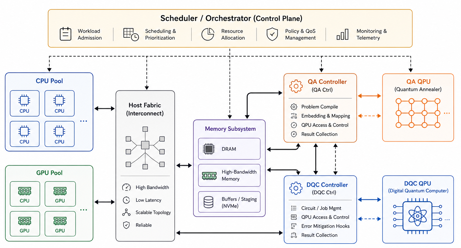
Figure 1 is the organizing object for HybridQC. An HCU is a configurable topology of compute nodes—classical CPUs/GPUs, memories, controllers, QA devices, DQC devices, and optional user-defined accelerators— connected by explicit data and control links. Workloads enter at the application layer as hybrid quantum-classical programs with per-job parameters, data payloads, and stage dependencies. The workload layer lowers those programs into multi-stage execution graphs. The runtime-profile layer attaches backend-specific QA and DQC service models. The topology layer determines where each stage can run and how data moves between nodes. Finally, the simulation layer executes the resulting stages over the topology and records resource utilization, data movement, queueing, wait, bottleneck, throughput, and completion metrics.
This layering is the first contribution of the paper: HybridQC models an HCU as a user-configurable topology rather than as a fixed backend template or a single QPU-runtime estimator. A user can change the topology without changing the workload definition, change a scheduling policy without changing backend profiles, or re-ground a backend profile with new hardware data without rewriting the execution engine. The four main input classes are summarized in Table 1. Appendices 8 and 11 record the concrete timing, controller, and link fields, while Appendix 10 expands the layered architecture in Figure 1.
| Input class | Role and configurable examples |
|---|---|
| Workload | Defines the multi-stage workload graph and data movement. Examples: family, shots, circuits, depth, QA/DQC payloads, and scaling axes. |
| Topology | Defines what stages can run and where contention occurs. Examples: resources, capacities, links, memory, controllers, and user-added nodes. |
| Control semantics | Defines programming, readout, mediation, and provider overhead. Examples: controller profile, routing mode, cross-device handoff mode, and cloud mode. |
| Execution config | Defines queue ordering, experiment scope, and feasibility checks. Examples: policy, arrivals, workload scale, horizon, and capacity semantics. |
3.2 Configurable Resource Graph↩︎
HybridQC separates the hardware object from the simulator that executes on it. A hybrid compute unit (HCU) is a directed resource graph \(G=(V,E)\). Nodes represent finite resources: CPU pools, GPU pools, memories, QA devices, DQC devices, QA controllers, DQC controllers, and user-defined accelerator or control nodes. We use the latter term for resources such as specialized controller processors, FPGAs, future QPU-specific mediators, or other accelerators that expose capacity and service-time fields but are not one of the default CPU/GPU/QA/DQC classes. Edges represent explicit data or control paths with latency, bandwidth, and routing constraints. A topology therefore specifies not only which QPUs exist, but how work reaches them and which controller resources serialize the path.
The resources in Figure 1 are not decorative. Each CPU, GPU, memory pool, controller, QA device, DQC device, and link can become the limiting resource for a different workload mix. The figure also shows why topology and scheduling are coupled: a scheduler can only relieve a bottleneck if the topology exposes alternate resources or sufficient controller/link capacity for work to move.
This graph representation is a design choice. It lets HybridQC ask architecture questions by editing the machine object itself: add DQC capacity, add a controller, widen a link, change memory limits, or introduce a new accelerator node. HybridQC then simulates how each workload stage reserves node capacity, moves data through links, and contributes to resource utilization over time, so the measured effect is tied to the declared topology rather than to a hand-coded benchmark variant.
Each resource node has a type, a capacity, and optional hardware limits. For classical nodes, these include memory capacity and device count. For QA and DQC nodes, they include problem-size limits such as available qubits, coupler/logical capacity, or backend-specific circuit limits. The full parameter table is kept in Appendix 8 because the values are detailed architectural inputs rather than the main conceptual contribution of this section. Section 4.4 explains how the QA/DQC timing terms are refined with backend-specific measurements.
3.3 Controllers and Links as First-Class Resources↩︎
Controllers are explicit resources in the graph, not hidden constants inside a QPU service time. A QA controller can serialize embedding submission, programming, readout, and result return. A DQC controller can serialize circuit submission, batched execution setup, readout, and feedback. Links are likewise explicit edges with latency, bandwidth, and routing constraints. Treating these components as first-class is what lets HybridQC distinguish a QPU bottleneck from a controller or interconnect bottleneck.
This distinction is essential for integrated HCU studies. If a workload adds DQC replicas but keeps one DQC controller, the simulator can expose the controller as the next limiting resource. If a workload grows output payloads, the simulator can charge the relevant link rather than hiding the transfer in a generic postprocessing constant. The evaluation uses this capability directly: the topology pair sweeps in Section [sec:results] show that QA-control replication and DQC-control replication optimize different objectives.
3.4 Configuration Interface↩︎
Listing [lst:hcu_config] illustrates the configuration interface. The syntax is intentionally compact. The contribution is that architectural choices are explicit and user-changeable. A user can add or remove resources, change controller concurrency, alter link bandwidth, select backend profiles, and switch scheduling policies without rewriting the simulator. More verbose profile, controller, and link variants are kept in Appendices 8 and 11.
Listing lst:hcu_config: Representative HCU~configuration used by HybridQC.
resources:
  - id: cpu_pool
    type: CPU
    count: 4
    memory_gb: 512
  - id: gpu_pool
    type: GPU
    count: 4
    model: NVIDIA_H100
    memory_gb: 80
  - id: qa_qpu
    type: QA
    backend_profile: dwave_advantage2
    max_qubits: 4600
  - id: dqc_qpu
    type: DQC
    backend_profile: ibm_kingston
    max_qubits: 156
  - id: qa_ctrl
    type: CONTROLLER
    target: qa_qpu
    concurrency: 1
  - id: dqc_ctrl
    type: CONTROLLER
    target: dqc_qpu
    concurrency: 1
links:
  - from: gpu_pool
    to: dqc_ctrl
    latency_us: 3.84
    bandwidth_gbps: 400
    chunk_bytes: 268435456
  - from: qa_ctrl
    to: dqc_ctrl
    latency_us: 12.0
    bandwidth_gbps: 100
execution:
  policy: HOBA
  cloud_overhead_mode: false
  workload_scale: 10
3.5 Capacity, Transfer, and Feasibility Semantics↩︎
Transfers are topology-aware. If a payload of \(B\) bytes crosses an edge with bandwidth \(\beta\) and latency \(\ell\), the nominal transfer time is \(T_{\mathrm{edge}}(B)=\ell+B/\beta\). Large-payload experiments cannot silently pass oversized data as one event. If the endpoint memory or controller buffer admits at most \(C\) bytes per transfer chunk, HybridQC charges latency per chunk: \[T_{\mathrm{edge}}(B)=\left\lceil B/C \right\rceil \ell + B/\beta.\] If a memory requirement exceeds capacity but the stage is streamable, the simulator models repeated chunks and sustained capacity use. If a quantum footprint exceeds the target backend and no decomposition is enabled, the row is marked infeasible rather than converted into a misleading runtime. Appendix 17.3 uses this distinction when reporting workload-scaling rows that complete, saturate, or become infeasible. These semantics are part of the HCU abstraction rather than an evaluation afterthought: without them, workload-scaling experiments would silently undercharge transfer and memory pressure.
4 HybridQC: Workloads, Grounding, and Simulator Design↩︎
The HCU abstraction in Section 3 defines the machine. This section defines the executable workload and timing choices that let the simulator use that machine. Each subsection is a design choice: how workloads are represented, which workload fields remain tunable, how workload scaling is applied, how measured backends parameterize stage service, and how the simulator executes and schedules the resulting stage graph.
4.1 System-Level Multi-Stage Simulation↩︎
HybridQC does not represent a hybrid workload as one quantum-service number because that would erase the resources that make topology matter. Instead, each job is lowered into a system-level multi-stage DAG whose nodes carry a resource type, runtime model, memory requirement, payload size, routing metadata, and predecessor dependencies. Classical stages reserve CPU/GPU nodes, QA and DQC stages reserve backend-profiled quantum nodes and controllers, and transfer stages move data across explicit links in the HCU topology. Problem mapping, embedding/transpilation, controller programming, readout, transfers, reconstruction, and postprocessing are explicit stages rather than hidden constants. Method-specific compiler, circuit-cutting, or QEM costs can be attached as additional parameterized stages when a workload provides them. The evaluation below does not claim a particular compiler, cutting algorithm, or mitigation implementation. In the implementation, each workload DAG is emitted as typed stage records that preserve resource needs, payload sizes, dependencies, and runtime-profile hooks.
This multi-stage representation is the bridge between the HCU abstraction in Section 3 and the execution engine described later in this section. The topology says what compute nodes and links exist. The stage graph says which nodes each job needs, what data must move between them, and which dependencies force serialization. This is why two workloads with similar QPU service time can have different end-to-end behavior. A portfolio workflow may be QA-to-DQC and transfer-heavy, a VQE workflow may be DQC-iteration-heavy, and a bin-packing workflow may mainly stress QA sampling and QA-controller staging. Appendix 12 gives the full workload taxonomy, stage definitions, runtime-model inputs, payload fields, and scaling semantics used to interpret the workload-scaling experiments.
| Class | Families | Representative stage graph |
|---|---|---|
| QA-heavy | bin packing [@de_Andoin_2022], vehicle routing [@maciejunes2025solvinglargescalevehiclerouting] | preprocessing, embedding, programming, QA sampling, result transfer |
| DQC-heavy | VQE [@peruzzo2014vqe], PES scan [@Brown_2024], job shop [@sawamura2025quantumclassicalhybridalgorithmusing], feature selection | transpilation, circuit execution, readout, reconstruction |
| Cross-modality | portfolio [@Morapakula_2025], unit commitment, transmission switching [@ellinas2024hybridquantumclassicalalgorithmmixedinteger], pipeline/SQC [@pipeline_optimization] | QA warm-start or search, transfer, DQC refinement, classical postprocessing |
| Mixed bundles | combinations of the above | independent typed DAGs co-scheduled on the same HCU |
3.5pt
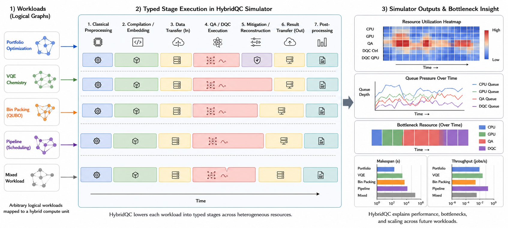
Figure 2 shows why the workload model is a system-level multi-stage graph rather than a scalar. The same logical job can generate CPU/GPU preprocessing, problem-mapping, quantum service, controller work, transfers, and reconstruction stages, and each of those stages can wait on a different resource. The figure therefore connects directly to the metrics in Section 3: utilization, stage wait, and bottleneck attribution are meaningful only because the simulator sees these stages separately. The evaluation later uses exactly these multi-stage records to explain why future data growth, shot growth, circuit growth, and depth growth produce different bottlenecks.
4.2 Workload Parameters↩︎
The second design choice is to keep workload parameters visible rather than collapsing them into one service-time multiplier. Table 2 groups the workload suite by architectural stress so that each family maps to a different region of the HCU design space. QA-heavy workloads primarily exercise embedding, programming, sampling, and QA result movement. DQC-heavy workloads stress transpilation, circuit execution, readout, and reconstruction. Cross-modality workloads are the most important for HCU studies because they use both quantum modalities and move intermediate data between them. Mixed bundles then co-schedule these families on the same topology, exposing contention that single-family runs can hide.
The quantitative ranges in Appendix Table ¿tbl:tab:workload95parameter95ranges? make the workload-scaling experiments interpretable. Shots, circuit count, depth, logical qubits, and payload size are not interchangeable knobs: QA shots primarily increase annealing service and readout demand. DQC circuit count and shots increase quantum-service demand. Depth changes circuit duration, and input/output payloads stress links, buffers, and memory. We keep the full numeric table in Appendix 12 so the main text can focus on the design choice rather than the full parameter grid.
4.3 Scaling Semantics↩︎
The third design choice is to scale workloads along explicit axes: data, shots, depth, circuit count, circuit-shot product, circuit-shot-depth product, and all fields. The workload-wide scale factor multiplies the workload’s compute and payload parameters before simulation, while communication-only scaling can separately stress input and output movement. This wording matters: 100\(\times\) data-only growth is not equivalent to 100\(\times\) growth in circuits, shots, and depth. Keeping these axes separate lets the simulator ask which hardware path becomes limiting as workloads grow. When large payloads no longer fit in one transfer or controller buffer, the chunked transfer semantics from Section 3 apply. Appendix 12 expands these scale modes, while Appendix 17.3 reports the completed and unfinished 100\(\times\) rows that result from applying them.
4.4 Hardware-Grounded Runtime Profiles↩︎
4.4.1 Backend-Specific Profiles↩︎
HybridQC uses backend-specific runtime profiles because the same stage graph should execute differently on different machines. Generic QA and DQC profiles provide defaults. Backend-specific profiles refine those defaults with measured data. The evaluation includes D-Wave Advantage 1 and Advantage 2 profiles and IBM Kingston, Marrakesh, and Fez profiles. Backend objects store not only fitted coefficients but also hardware metadata such as qubit counts, timing fields, embedding status, transpiled circuit properties, and provider-result fields. This makes profiles auditable and re-groundable as new measurements arrive.
The grounding step supports the third contribution of the paper: live hardware measurements are used to parameterize the service models consumed by the HCU simulator. The point is not to claim that a single global formula predicts all future machines. The point is to make backend assumptions explicit, backend-specific, and replaceable. Appendix 15 lists the hardware campaigns, and Appendix 16 gives the fit rows and coefficients behind the compact validation result.
4.4.2 Physical Occupancy versus Cloud Wall Time↩︎
For D-Wave, the physical occupancy target is QPU access time. Programming, anneal, readout, delay, sampling, embedding status, and wall time are retained as separate fields. For IBM, the physical occupancy target is IBM-reported quantum seconds, fitted from circuit count, shots, qubits, depth, transpiled depth, two-qubit gates, backend, and circuit family. Queue and provider wall fields are used only in optional cloud-proxy mode. Thus the same hardware records can validate today’s cloud-access behavior without forcing future integrated HCUs to inherit cloud overhead as a device constant. The full target/predictor mapping is in Appendix 16 (Table 6).
4.4.3 Grounding Campaigns and Simulation Interface↩︎
The grounding campaigns are designed around the simulator interface rather than around isolated benchmark curves. Broad calibration grids span problem size, circuit shape, backend, shot/read count, and timing fields so that backend profiles have enough variation to fit service-time coefficients. Workload-shaped rows such as portfolio, pipeline, PES scan, and VQE are retained separately so the fitted profiles can be checked against application-shaped artifacts rather than only synthetic sweeps. Appendix Tables ¿tbl:tab:ibm95grid95app?–¿tbl:tab:dwave95timing95decomposition95app? record the complete grid coverage, timing fields, and workload-shaped rows. After fitting, each backend profile supplies service-time estimates to the typed stages described in Section 4: stage graphs determine where a job needs service, while backend profiles determine how long each QA or DQC reservation occupies the HCU. Integrated-mode runs use calibrated physical service. Cloud-proxy runs add provider overhead when reproducing today’s cloud execution. Appendix 16 gives the numerical timing decomposition behind this separation.
4.5 Simulator Design and Policy Co-Design↩︎
4.5.1 Execution Pipeline↩︎
The execution engine is designed to preserve the same resource semantics introduced above. HybridQC takes a workload list, applies workload-scaling parameters, lowers each job into typed stages, routes payloads through the HCU graph, and runs a discrete-event simulation until all jobs complete or the horizon is reached. Stage starts and completions update resource state, queues, memory occupancy, and metric accumulators. This design makes end-to-end workload behavior visible: a DQC-heavy job can still be delayed by problem-preparation, data movement, controller availability, or reconstruction.
The implementation has two cooperating layers. The Python pipeline is the canonical model: it owns workload construction, backend-profile loading, subroutine expansion, measurement records, and experiment orchestration. The Rust native engine executes the typed event path used for large sweeps. This split keeps the model inspectable while allowing the hot event loop, typed queues, and metric accumulation to run without Python object churn. Section 5 defines the implementation-aligned diagnostic metrics used in the evaluation tables.
4.5.2 Typed Stages and Subroutines↩︎
Problem preparation, embedding/transpilation, QA execution, DQC execution, controller programming/readout, transfers, reconstruction, and postprocessing are represented as typed stages. This is a design choice because these subroutines consume different resources and can become bottlenecks independently. The typed representation avoids treating subroutines as opaque constants and makes the implementation testable: backend profiles can be validated against QA/DQC timing data, stage expansions can be checked independently, and policies can be tested against explicit queue states. Compiler-specific, circuit-cutting, and QEM methods are extensibility points that can be modeled as additional parameterized stages, but they are not method-specific claims in this evaluation.
4.5.3 Scheduling as a Topology Knob↩︎
Topology and scheduling are coupled: the topology defines which resources can become scarce, while the policy decides which ready stage receives a scarce controller, QPU, link, or classical resource next. HybridQC therefore treats policy choice as part of the HCU configuration rather than as an implementation detail.
The evaluated policies span different scheduling aims. First-In, First-Out (FIFO) is the arrival-order baseline. Timeout batching releases QA and DQC controller batches once either a size or wait threshold is reached. Hybrid Overhead-Balanced Adaptive (HOBA) uses queue-aware dispatch and batching to protect constrained quantum paths. Adaptive Batch-Optimal (ABO) uses arrival-rate-aware batching, while Greedy Max Pressure (GMP) and Max-Pressure prioritize work expected to relieve downstream queues. The systems claim is not that this policy set is exhaustive. It is that policy and topology must be evaluated together. A policy that helps a DQC-heavy mix may not help a QA-heavy workload, and adding QPU capacity may not improve throughput if the policy still serializes work through one controller. Appendix 14 gives the expanded policy names, state, scoring rules, and tie-breaking behavior. The mixed-policy result rows are summarized in Appendix 17.4.
5 Evaluation and Results↩︎
5.1 Methodology and HybridQC Design Questions↩︎
The evaluation separates validation from forecasting. Validation asks whether the multi-stage runtime models used by HybridQC are compatible with live hardware measurements. Forecasting asks what those grounded models imply for full hybrid workloads running on proposed tightly integrated topologies. This split is the point of the simulator: measured hardware validates the service models, then the validated models let us study HCUs and workload scales that do not exist today. The evaluated workload stages include problem preparation, embedding or transpilation, controller programming/readout, QA/DQC execution, transfers, reconstruction, postprocessing, memory capacity, queues, and scheduling policies. Compiler-specific, circuit-cutting, and QEM algorithms are supported as parameterized stage extensions, but are not evaluated as named methods in this paper. The workload suite is summarized in Table 2: QA-heavy optimization, DQC-heavy circuit workloads, cross-modality QA-to-DQC workflows, and mixed bundles. Appendix Table ¿tbl:tab:workload95parameter95ranges? gives the full numeric parameter ranges.
We organize the evaluation around the following questions.
V1: Hardware grounding. Can backend-specific QA and DQC service models fit measured D-Wave access time and IBM-reported quantum seconds well enough to support system-level and multi-stage simulation?
V2 (Appendix 17.2): Cloud versus integrated execution. Does separating physical QPU occupancy from provider wall time change architectural conclusions?
E1: Topology balance. When additional hardware is available, does adding one resource class suffice, or do workloads require balanced scaling across classical, quantum, controller, and link resources?
E2: Scheduling. Do queueing policies materially affect throughput and bottleneck migration for mixed hybrid workloads?
E3 (Appendix 17.4): Mixed-workload stress. What bottlenecks appear only when heterogeneous workload families share the same HCU?
E4 (Appendix 17.5): QA load amplification. When does extra QA sampling reduce DQC fallback pressure?
E5 (Appendix [app:e595sensitivity95extensions]): Sensitivity extensions. How do controller/link variants affect bottlenecks?
S1: Workload scaling. Which scaling axes are benign and which axes produce architectural saturation at 10\(\times\) and 100\(\times\) growth?
The main text answers the central validation, topology, policy, and workload-scaling questions. The appendix answers deployment-mode, mixed-workload, load-amplification, and sensitivity questions with numerical rows. The following result subsections use the same V/E/S identifiers as the question list.
5.2 Implementation and Experiment Inputs↩︎
The implementation path mirrors the simulator design in Section 4.5. A Python front end defines workload families, HCU topologies, backend profiles, hardware-grounding parsers, experiment manifests, and analysis scripts. A Rust execution engine runs the large typed-event sweeps and emits the metrics reported below. IBM grounding uses Qiskit/Runtime artifacts [@qiskit_zenodo; @ibm_estimate_runtime; @ibm_sessions]; D-Wave uses Ocean SampleSets [@dwave_ocean_sdk]. Each experiment specifies a workload bundle, backend/profile metadata, scaling or shot/read parameters, HCU graph, policy, and timing fields. The same workload families generate the IBM circuits and D-Wave QUBOs used for grounding, keeping calibration tied to simulated workloads. Policy scoring rules, hardware grids, backend metadata, and dense supporting sweeps are provided in the appendix.
5.3 Hardware-Grounding Data↩︎
For D-Wave, we generate QUBO and workload-derived instances for Advantage 1 and Advantage 2 and record hardware metadata, embedding outcome, wall time, QPU access time, programming time, readout time, sampling time, sample counts, and problem structure. The primary physical-occupancy target is QPU access time. Wall time is retained as a cloud-overhead observation rather than folded into the device service model.
For IBM, we generate circuits across qubit count, depth, shot count, and circuit family for Kingston, Marrakesh, and Fez. The primary physical occupancy target is IBM-reported quantum seconds. We retain backend metadata, transpiled circuit properties, queue/provider timing fields when available, and result payloads so that backend profiles can be refit or extended without rerunning all jobs.
For each backend profile, we report mean absolute percentage error (MAPE) and coefficient of determination (\(R^2\)) on the physical-occupancy target used by the simulator. For measured target \(y_i\) (hardware runtime) and prediction \(\hat{y}_i\) (HybridQC runtime), \(\mathrm{MAPE}=(100/n)\sum_i |(y_i-\hat{y}_i)/y_i|\), computed on positive timing targets, and \(R^2=1-\sum_i(y_i-\hat{y}_i)^2/\sum_i(y_i-\bar{y})^2\), which measures the fraction of target variance explained by the fitted profile. These definitions are used by the grounding anchors below.
5.4 Evaluation Metrics↩︎
HybridQC reports only implementation metrics used in the results. Let \(J\) be the submitted jobs, \(J_c\) the completed jobs, \(A_j\) and \(C_j\) the arrival and completion times, and \(T_0=\min_j A_j\). The reported run makespan is total_time_s: \(T_{\mathrm{run}}=\max_{j\in
J_c}C_j-T_0\). Per-job completion time is \(T_j=C_j-A_j\). makespan_p95_s is \(Q_{0.95}(\{T_j:j\in J_c\})\) and is used for tail-latency plots. Throughput is \(\Theta=|J_c|/T_{\mathrm{run}}\). Completion ratio \(\rho_{\mathrm{done}}=|J_c|/|J|\) marks unfinished workload-scaling rows as capacity/horizon signals. For a resource class \(r\), the active-wall critical path fraction (CPF) is \(\phi_r=B^{\mathrm{wall}}_r/T_{\mathrm{run}}\), reported in the cpf_\(r\) or
active-utilization fields. The bottleneck class is \(\arg\max_r \phi_r\). Capacity-normalized utilization is \(U_r=B_r/(T_{\mathrm{run}}\mathrm{cap}_r)\) and is used only where the results
explicitly report utilization curves.
The result subsections below follow the evaluation questions above. Each subsection states the compact claim in the main text and points to the appendix rows that make the claim auditable. The order mirrors the paper’s contributions: hardware-grounded profiles first, then topology and policy co-design, then workload-scaling analysis. Appendix 17.2, Appendix 17.4, and Appendix [app:e595sensitivity95extensions] answer the deployment-mode, mixed-workload, load-amplification, and sensitivity-extension questions from Section 5.
5.5 V1: Hardware Grounding Is Accurate Enough for System-Level and Multi-Stage Simulation↩︎
Table 3 reports compact validation anchors. For D-Wave, the best Advantage 2 training fit reaches 3.92% MAPE and \(R^2=0.981\) for QPU access time. The current workload-validation fit for Advantage 1 reaches 8.04% MAPE and \(R^2=0.994\). For IBM, Fez reaches 5.26% MAPE on its backend campaign, Kingston reaches 16.45% MAPE with the transpiled augmented model, and Marrakesh reaches 19.01% MAPE. These are multi-stage service fits, using the metrics defined in Section 5. They are not fits to end-to-end cloud wall time: cloud wall time includes queueing, provider orchestration, client overhead, and network effects that vary across submissions and are modeled separately from physical QPU occupancy.
The result supports the first validation claim: hardware measurements can ground the QA and DQC occupancy models used by HybridQC. It also shows why backend profiles must be explicit. Kingston, Marrakesh, and Fez differ enough that a single global IBM coefficient set would hide backend-specific behavior. The same is true for D-Wave Advantage 1 versus Advantage 2: the profiles share a generic QA structure, but the fitted parameters and hardware metadata should remain backend-specific. Appendices 15 and 16 provide the full hardware grid coverage, workload-shaped validation rows, fit diagnostics, and timing decompositions behind these compact anchors.
| Backend | Timing target | Rows | MAPE (%) | \(R^2\) |
|---|---|---|---|---|
| D-Wave Adv.-1 | QPU access time | 240 | 8.04 | 0.994 |
| D-Wave Adv.-2 | QPU access time | 263 | 3.92 | 0.981 |
| IBM Fez | quantum seconds | 7 | 5.26 | 0.978 |
| IBM Kingston | quantum seconds | 80 | 16.45 | 0.978 |
| IBM Marrakesh | quantum seconds | 21 | 19.01 | 0.967 |
2.4pt
5.5.0.1 Insight.
The simulator should not use provider wall time as physical QPU occupancy. For D-Wave, QPU access time is the right resource-locking target. Wall time is better modeled as cloud/client overhead. For IBM, the right DQC-service target is IBM-reported quantum seconds, while queue and orchestration fields remain deployment overheads. This separation is central to using current cloud data to forecast future tightly integrated systems.
5.6 E1: Balanced Topologies Matter More Than Isolated QPU Scaling↩︎
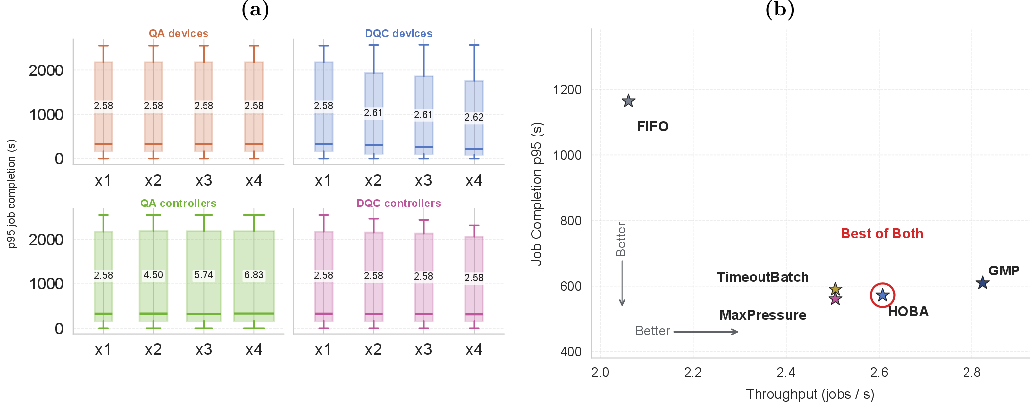
Figure 3 (a) shows why HybridQC models the whole HCU rather than only QPU count. The sweep uses the true workload families in Table 2: QA-heavy, DQC-heavy, cross-modality, and mixed bundles. Its four panels separately replicate QA devices, DQC devices, QA controllers, and DQC controllers. Colors distinguish those swept resource classes. The labels x1–x4 denote the total number of instances of the swept resource class, where x1 is the baseline and x4 is the four-replica variant. Repeated 2.58 jobs/s entries appear in both the QA and DQC-controller sweeps: for those workloads, the swept resource is not on the active bottleneck path, so adding replicas leaves average throughput unchanged. The detailed active-time diagnostic views that explain bottleneck migration are moved to Appendix 17.1 (Figures 6 and 7).
The first topology result is that the largest payoff does not always come from replicating the quantum device itself. Moving from one to four QA-controller replicas improves throughput by 164% while changing p95 completion time by only \(-2\) s. Replicating DQC devices alone improves throughput by roughly 1%, but controller active time rises as DQC replicas are added. Thus Figure 3 (a) shows broad replica payoff, while the appendix mechanism plots show why QPU scaling helps most when the matching controller path scales with it. The balanced 10\(\times\) topology remains the best variant, but its speedup is 2.19–3.42\(\times\), not 10\(\times\).
The pair-sweep data sharpen this result without needing another main-text matrix. QA-controller replication gives the strongest throughput improvement: average throughput increases from 2.85 to 9.75 jobs/s, a 3.43\(\times\) gain, while p95 completion time changes little. DQC-controller replication gives the stronger tail-latency improvement: p95 completion time falls from 7601 s to 6348 s, about 16.5%, while throughput changes by only about 1%. Thus the best topology extension depends on the objective. A QPU-only model would miss this split because the critical resource is often the controller path rather than the QPU itself. Appendix 17.1 keeps the corresponding pair-sweep numerical summary for auditability.
5.6.0.1 Insight.
Adding only quantum capacity can be the wrong investment: DQC-heavy workloads can remain controller- or reconstruction-limited, QA-heavy workloads can remain embedding- or transfer-limited, and mixed workloads can expose both. The appendix policy/topology summary in Appendix [app:policy95topology95matrices] preserves the key unbalanced variants that do not fit in the main text.
5.7 E2: Scheduling Policy Changes Throughput and Bottleneck Migration↩︎
Scheduling changes the mixed-workload result because policies use different signals when several ready stages compete for the same HCU resource. FIFO is the arrival-order baseline. HOBA is the Hybrid Overhead-Balanced Adaptive policy, which uses queue-aware dispatch and batching to protect constrained quantum paths. ABO is the Adaptive Batch-Optimal policy, which batches from observed arrival rates and setup costs. Greedy Max Pressure (GMP) and Max-Pressure prioritize stages that relieve downstream queues or pressure points. The full scoring rules and tie-breaking behavior are in Appendix 14. The main-text result focuses on how those policy choices change the system outcome.
Figure 3 (b) shows that FIFO has the lowest throughput and highest tail latency in the aggregate policy sweep, while GMP has the highest throughput. The active-time decomposition in Appendix 17.1 (Figure 8) shows the supporting mechanism: different policies shift bottleneck pressure across QA, DQC, controller, transfer, and classical components rather than merely changing a single queue order. At 20 jobs per workload, HOBA finishes in 3812.66 s, Max-Pressure in 4876.15 s, and FIFO in 6862.32 s. Thus HOBA is 1.80\(\times\) faster than FIFO for this stress case. The best policy is not universal: GMP is best for bin packing, HOBA for portfolio, and Max-Pressure for PES scan and the 10-job mixed workload.
5.7.0.1 Insight.
Policy value depends on workload composition. FIFO is useful as a baseline, but pressure-aware and bottleneck-aware policies can improve throughput when they see the right signal and can over-prioritize the wrong queue when bottlenecks shift. This motivates simulating policy and topology together. Appendix 14 gives the policy scoring signals, and Appendix 17.4 reports the full policy-by-workload matrix behind this summary.
5.8 S1: Workload Scaling Is Multi-Axis↩︎
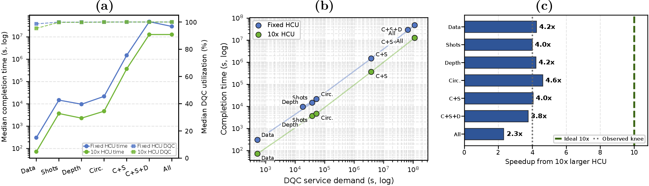
S1 scales the workload families in Table 2, with full field ranges in Appendix Table ¿tbl:tab:workload95parameter95ranges?: QA optimization, DQC circuit workloads, cross-modality QA+DQC workflows, and mixed bundles sharing the same HCU. The largest current DQC rows in the appendix have up to 72 logical qubits and depth 2,000, so 10\(\times\) and 100\(\times\) all-field scaling stress future systems with hundreds to thousands of logical qubits and depths up to 200,000 rather than hardware that exists today. The strongest scaling result is that growth is not one-dimensional. At 100\(\times\) data-only scaling on the fixed machine, median runtime is about 306 s. At 100\(\times\) circuits-shots-depth scaling, it reaches about \(4.806\times 10^7\) s on the fixed machine and \(1.280\times 10^7\) s on the 10\(\times\) larger machine. Figure 4 (a) separates these axes, while Figure 4 (b) shows how those axes move the bottleneck. QA-only workloads grow much more slowly than DQC-only and mixed QA+DQC workloads under multi-axis workload scaling. The large values are not a transfer artifact. They come from DQC growth where circuit count, shots, and depth multiply. Infeasible 100\(\times\) all-fields rows are reported separately as capacity failures, not as completed runtime ratios.
Figure 4 (b) explains why the larger HCU does not recover ideal scaling: circuits, shots, and depth move points along the same DQC-dominated trajectory, so balanced capacity lowers runtime without changing the root cause of saturation.
Figure 4 (c) quantifies the compromise. At 100\(\times\) workload scale, the 10\(\times\) larger HCU improves median runtime by 4.24\(\times\) for data-only growth, 4.62\(\times\) for circuit-only growth, 4.05\(\times\) for circuits-and-shots growth, 3.75\(\times\) for circuits-shots-depth growth, and 2.31\(\times\) for all-fields growth. The larger topology helps most when the scaled workload exposes parallel work, but it does not produce linear speedup when multiple DQC execution axes grow together.
5.8.0.1 Insight.
Workload-scaling studies should report the scaling axis, not only the scale factor. Data-only scaling mostly stresses transfer, memory, and preprocessing, whereas circuits-shots-depth scaling multiplies submitted circuits, shots per circuit, and circuit depth. HybridQC turns that ambiguity into an experiment by scaling workload fields separately and recording which resources saturate. Appendix 17.3 contains the representative completed 100\(\times\) rows in Table ¿tbl:tab:future95workload95numeric95app? and summarizes the unfinished fixed-HCU capacity-boundary rows in prose. The main-text bottleneck migration and compromise analyses show that balanced machine growth helps but does not erase multiplicative DQC pressure.
6 Discussion and Limitations↩︎
HybridQC is designed for topology-level reasoning, not quantum-state simulation. It asks what happens when staged hybrid workloads contend for a proposed machine, preserving stage graphs, finite queues, payloads, controllers, and transfer routes. This exposes effects that kernel timing hides: non-linear scaling, policy-dependent throughput, cloud overhead separate from physical occupancy, and workload growth that depends on which fields scale.
This validation-to-forecasting split is intentional. Hardware measurements are used to make the service models credible at today’s scale, while the simulator uses those calibrated models to ask architecture questions that cannot yet be measured directly, such as how controller, link, and scheduling bottlenecks move in future local-accelerator HCUs.
The main limitations are scope and extrapolation. HybridQC is not a circuit-state simulator, annealing solver, quantum-control compiler, or provider Runtime replacement. It consumes circuit/QUBO properties, backend measurements, topology definitions, and stage graphs. The fitted QA/DQC service models reflect the hardware data collected here, but future backends, provider queues, circuit families, embedding outcomes, and algorithmic accuracy require new calibration. Workload scaling is therefore a controlled stress test: capacity-infeasible rows are architecture warnings under the configured memory, transfer, and resource constraints, not universal predictions.
7 Conclusion↩︎
HybridQC provides a hardware-grounded simulator for tightly integrated hybrid quantum-classical systems. By validating service models on live IBM and D-Wave measurements and applying them through a topology-aware discrete-event engine, it lets researchers evaluate full hybrid workloads and forecast bottlenecks in machines that do not yet exist. The evaluation shows that backend-specific profiles can ground system-level QA and DQC occupancy, that balanced resource scaling is more effective than isolated QPU scaling, that scheduling policy changes mixed-workload throughput, and that cloud wall time should be separated from physical resource occupancy. It also shows that future workload scaling must be described by axes: data-only scaling is mild, while joint growth in circuit count, shots, and depth can saturate DQC resources by orders of magnitude. HybridQC therefore offers a practical path for validating today’s hybrid workloads and forecasting tomorrow’s architecture bottlenecks.
8 Baseline Timing Parameters↩︎
Table ¿tbl:tab:hcu95parameters95exact95app? records the original baseline timing parameters used to instantiate a concrete HCU. The current paper’s backend-specific profiles refine these priors with IBM and D-Wave measurements (Section 4.4), but the table is useful because it makes the simulation assumptions explicit: physical QPU occupancy, controller staging, transfer, and architectural constraints are separate terms.
5pt
@p0.30p0.62@ Parameter & Value used or modeled
GPU–QPU bandwidth & 400 Gb/s, approximately 50 GB/s [@nvidia_nvqlink]
GPU–QPU latency & mean 3.84 \(\mu\)s, max 3.96 \(\mu\)s [@nvidia_nvqlink_blog]
Transfer model & \(T_{\text{link}}(S)=3.84\,\mu\mathrm{s}
+ S/(50\,\mathrm{GB/s})\) before chunking. Chunked transfers charge latency per chunk when endpoint buffers are smaller than the payload.
Programming time \(T_{\text{program}}\) & 17.7 ms [@dwave_qpu_properties]
Anneal time \(T_{\text{anneal}}\) & 0.5–2000 \(\mu\)s [@dwave_qpu_properties]
Readout time \(T_{\text{readout}}\) & 17–265 \(\mu\)s [@dwave-annealing]
Per-sample delay \(T_{\text{delay}}\) & 20.6 \(\mu\)s [@dwave_qpu_properties]
Reads per QA job & workload-dependent, 200–2200 in the workload table.
QA job-time structure & \(T_{\text{program}}+N_{\text{reads}}
(T_{\text{anneal}}+T_{\text{readout}}+T_{\text{delay}})\), refined by backend-specific QPU-access fits in the hardware-grounded profiles.
Sub-job overhead \(T_{\text{overhead}}\) & 2.0 s [@ibm_estimate_runtime]
Repetition delay & 250 \(\mu\)s [@ibm_estimate_runtime]
Gate-time prior & 100 ns [@ibm-quantum-qpu-information]
Circuit duration prior & \(T_{\text{gate}}\times\text{circuit width/depth
proxy}\), replaced in the calibrated model by circuit family, depth, transpiled depth, gate counts, qubits, and shots.
Circuits per DQC job & workload-dependent, 8–128 in the original HCU workload ranges and refined by the current workload registry.
Shots per circuit & workload-dependent, 50–1200 in the original HCU ranges and refined by current generated circuits.
DQC job-time structure & \(T_{\text{overhead}}+(T_{\text{circuit}}+\text{rep\_delay})\cdot N_{\text{exec}}\), with IBM-reported quantum seconds used as the calibrated service target.
QA input/output payloads & 4–40 KB / 4–32 KB in the original compact parameterization. Current workload table exposes per-workload payload ranges.
DQC input/output payloads & 4–200 KB / 4–40 KB in the original compact parameterization. Current workloads include larger generated payloads such as portfolio and PES scan rows.
QA\(\rightarrow\)DQC direct path & not available by default. Cross-modal workflows are host/controller mediated unless a topology explicitly declares a controller cross-link or direct QPU link.
QPU lock semantics & exclusive during physical quantum execution and programming/readout intervals charged by the backend profile.
9 Hardware-Grounding Equations↩︎
This section collects the equations used to turn measured IBM and D-Wave rows into simulator service profiles. The main text uses the fitted profiles. The appendix records the modeling choices so that the validation claims are auditable. The most important convention is that physical device occupancy and cloud/provider wall time are separate quantities. The simulator uses physical QPU occupancy for tightly integrated HCU forecasts and exposes provider wall time as an optional cloud-execution mode.
9.0.0.1 Chunked transfer model.
For a payload of size \(S\) bytes crossing a link with one-way latency \(\ell\) and bandwidth \(B\), the unchunked service time is \[T_{\mathrm{tx}}(S)=\ell+\frac{S}{B}.\] When a link endpoint or controller buffer limits each transfer to \(C\) bytes, the simulator charges one latency per chunk: \[n=\left\lceil\frac{S}{C}\right\rceil,\qquad T_{\mathrm{tx,chunked}}(S)=n\ell+\frac{S}{B}.\] This is the mechanism that prevents large scaled payloads from being treated as if they fit through a link or controller in one zero-cost movement.
9.0.0.2 D-Wave QA physical-access model.
The baseline QA service decomposition is \[T_{\mathrm{QA}} = T_{\mathrm{program}}+ R\left(T_{\mathrm{anneal}}+T_{\mathrm{readout}}+T_{\mathrm{delay}}\right),\] where \(R\) is the number of reads. Backend-specific profiles refine these terms with measured D-Wave QPU-access time. Provider wall time is retained as a separate cloud-overhead observable and is not treated as physical QPU occupancy.
9.0.0.3 IBM Runtime quantum-seconds model.
For IBM backends, the fitted target is IBM-reported quantum seconds rather than client wall time. The coefficient table later in this appendix uses the feature form \[q = a+bN_{\mathrm{circuits}} c\frac{S}{1000} d\frac{(\sum_i D_i)S}{10^6} e\frac{(\sum_i Q_iD_i)S}{10^8},\] where \(S\) is shots, \(D_i\) is depth, and \(Q_i\) is qubit count for circuit \(i\). The fitted constants are backend specific. The equation gives the feature semantics.
9.0.0.4 QA load-shedding success model.
For D-Wave SampleSet grounding, each QUBO size/degree group has an empirical best observed energy \(E^\star_g\). A returned sample \(x\) is a success at relative energy-gap target \(\epsilon\) if \[H_\epsilon(x)= \mathbf{1}\left[ \frac{E(x)-E^\star_g}{\max(1,|E^\star_g|)}\le \epsilon \right].\] The measured hit probability is weighted by occurrence count: \[\hat{p}_\epsilon = \frac{\sum_x n_x H_\epsilon(x)}{\sum_x n_x}.\] For an amplification cap \(A\) relative to a base QA attempt, the independent attempt approximation gives \[P_{\mathrm{success}}(A)=1-(1-\hat{p}_\epsilon)^A, \qquad P_{\mathrm{fallback}}(A)=(1-\hat{p}_\epsilon)^A .\] The break-even DQC fallback time for increasing from \(A_0\) to \(A_1\) is \[T_{\mathrm{DQC,break}} = \frac{T_{\mathrm{QA}}(A_1)-T_{\mathrm{QA}}(A_0)}{P_{\mathrm{fallback}}(A_0)-P_{\mathrm{fallback}}(A_1)}.\] This is the fallback service time above which the additional QA attempts pay off in expected service time. It is a policy input, not a claim that every QA workload should always be amplified.
10 Layered HCU Architecture Details↩︎
The main text keeps the system model compact. It is the expanded version of the layered description in Section 3: application stages, control resources, hardware links, and simulation metrics are separated so that changing one layer does not require rewriting the others.
10.0.0.1 Application layer.
Workloads are expressed as staged hybrid workflows rather than single quantum calls. The canonical modes are QA-only optimization, DQC-only circuit execution, QA-to-DQC refinement, and QA with classical mediation. Cross-modal jobs are host- and controller-mediated by default: QA results return through readout, controller, host/GPU, and transfer stages before DQC refinement is submitted. This prevents the simulator from assuming a direct QA-to-DQC path unless the topology explicitly provides one.
10.0.0.2 Control layer.
Controllers are finite-capacity service resources. They can model host relay, controller-side processing, controller-to-controller cross-links, cryogenic edge control, hierarchical controller meshes, QPU-direct paths, and full bypass modes. A quantum segment is therefore decomposed into transfer-in, controller service, physical execution, controller readout/return, and transfer-out terms: \[\begin{align} T_{\mathrm{QA}} &= T_{\mathrm{in,QA}} + T_{\mathrm{QA,ctrl}} + T_{\mathrm{QA,exec}} \notag\\ &\quad + T_{\mathrm{QA,ctrl,out}} + T_{\mathrm{out,QA}}, \\ T_{\mathrm{DQC}} &= T_{\mathrm{in,DQC}} + T_{\mathrm{DQC,ctrl}} + T_{\mathrm{DQC,exec}} \notag\\ &\quad + T_{\mathrm{DQC,ctrl,out}} + T_{\mathrm{out,DQC}} . \end{align}\] The main evaluation uses this decomposition with QEC disabled so that the reported effects isolate the general HCU simulator rather than specialized QEC execution machinery.
10.0.0.3 Hardware layer.
The link model supports host-side links such as NVQLink, PCIe Gen4/Gen5, InfiniBand NDR400, and 100G Ethernet, plus controller/QPU links such as cryogenic coax, cryogenic CMOS, and photonic-control profiles. Cross-modality connectivity can be mediated-only, controller-cross-linked, or direct if the user declares such a path. Resource replication creates additional resources with the same profile and connects replicas according to the declared routing mode.
10.0.0.4 Simulation layer.
HybridQC executes a workload-stage DAG over an HCU resource graph. Stage dependencies define readiness. Resource capacities and queues define when a ready stage can start. The simulator updates resource occupancy, stage wait, average queue-length diagnostics, memory/buffer state, transfer service, and subroutine service as events complete.
11 Controller, Link, and Jitter Profiles↩︎
The main paper uses controller and link profiles to show that HybridQC can model many HCU designs without changing the workload definitions. This appendix records the profile space used by the legacy HCU study and retained by the current simulator. These variants support the topology-extensibility claim in Section 3: users can test host relay, controller mediation, cross-links, bypass modes, and different interconnect families by changing the configuration, not the workload.
Tables 4 and 5 should be read together. The first table defines the routing semantics for cross-modal handoff, while the second defines the link families whose latency, bandwidth, and chunking behavior make those semantics measurable in the simulator.
| Control variant | Required topology feature | Interpretation |
|---|---|---|
| Host relay | host/controller paths | QA-to-DQC handoff returns through the host before later quantum submission. |
| Controller processing | controller-local service | Mediation stays in the control plane but still consumes controller capacity. |
| Controller-to-controller | QA/DQC controller cross-link | Handoff uses a declared control-plane edge rather than the full host path. |
| Cryogenic edge control | near-device controller profile | Reduced controller turnaround through more capable near-device control. |
| Hierarchical mesh | controller cross-link plus coordination | A deeper controller hierarchy coordinates cross-modal handoff. |
| QPU direct | QA-to-DQC edge | The topology exposes a direct quantum-device handoff path while preserving downstream accounting. |
| Full bypass | QA-to-DQC edge plus bypass semantics | Direct path bypasses selected downstream staging/readout terms when enabled. |
| Link/profile family | Examples | Modeled effect |
|---|---|---|
| Host-side accelerator links | NVQLink [@nvidia_nvqlink; @nvidia_nvqlink_blog], PCIe Gen4/Gen5, InfiniBand NDR400, 100G Ethernet | Host/controller and host/accelerator transfer latency, bandwidth, and chunked payload movement. |
| Controller/QPU links | cryogenic coax, cryogenic CMOS, photonic control [@classsical_control_electronics; @classical_interfaces_control; @quantum_control_fpga] | Near-device programming, readout, and control transport. |
| Cross-modality links | mediated-only, controller cross-link, direct QPU link | Whether QA-to-DQC handoff must return through the host or can use a shorter declared path. |
| Replicated links | complete routing across replicated resources | Capacity scaling through additional resources rather than magically enlarging one device. |
11.0.0.1 Jitter model.
When jitter is enabled, HybridQC perturbs only the latency term of selected host-side links. Let \(\ell_0\) be the nominal link latency and \(J\sim\mathcal{N}(1,\mathrm{CV})\) be a multiplicative jitter factor. The simulator uses \[\ell'=\max(\epsilon,\ell_0J), \qquad T_{\mathrm{tx}}(S)=\ell' + \frac{S}{B},\] where \(S\) is payload size, \(B\) is bandwidth, and \(\epsilon\) prevents negative latency. A coefficient of variation of 0.05 corresponds to roughly 5% relative latency variation. The main evaluation uses deterministic profiles unless a jitter ablation is explicitly reported.
12 Workload Definitions and Scaling↩︎
The workload suite is organized by modality. QA-heavy workloads include bin-packing, vehicle-routing, and related QUBO instances. DQC-heavy workloads include VQE, QAOA-style sparse circuits, feature-selection circuits, and PES scan. Cross-modality workloads include portfolio optimization, unit commitment, transmission switching, pipeline/SQC-style workflows, and mixed bundles that combine families in the same HCU.
This block expands Section 4. The main text keeps the workload table readable. The appendix explains how those workloads map to modality classes and why scaling is applied by named axes instead of by one generic “problem-size” multiplier.
The main text keeps the workload-family summary compact. This appendix records the quantitative parameter ranges and scaling definitions that make the main-text rows auditable: QA-heavy families stress QUBO size, reads, QA-controller staging, and result movement. DQC-heavy families stress circuit count, shots, depth, controller readout, and reconstruction. Cross-modality and mixed bundles combine those paths on shared resources, exposing transfer, controller contention, and bottleneck migration.
3.5pt max width=
12.0.0.1 Stage and runtime definitions.
Each workload is lowered into typed stages. A stage definition records:
the stage name, such as preprocessing, problem mapping, embedding/transpilation, QA execution, DQC execution, controller programming/readout, transfer, reconstruction, or postprocessing.
the target resource class or explicit device binding.
a runtime model, which may be a fixed service term, a fitted QA/DQC backend profile, a payload-transfer model, or a subroutine model.
memory and payload fields used by capacity and transfer semantics.
predecessor dependencies that form the multi-stage workload graph.
QA stages consume backend-specific QPU-access profiles, DQC stages consume backend-specific quantum-second profiles, and transfer stages use the link equations in Section 3. Controller programming/readout, reconstruction, and postprocessing are represented as explicit stage expansions so their service and wait time can be attributed separately. Compiler-specific, circuit-cutting, and QEM stages can be added as parameterized extensions when a workload supplies those methods. The reported evaluation does not depend on a named compiler, cutting algorithm, or QEM implementation.
Table ¿tbl:tab:workload95parameter95ranges? gives the full parameter ranges used by the workload generator. The scaling semantics below explain how those fields are multiplied in the future-workload experiments.
Scaling is applied to named workload axes rather than to a single ambiguous “problem size.” The evaluation distinguishes:
data-only scaling, which increases payload and memory pressure.
shot-only scaling, which increases repeated DQC/QA measurement demand.
depth-only scaling, which increases circuit service time.
circuit-only scaling, which increases the number of submitted quantum kernels.
circuit-shot and circuit-shot-depth scaling, which multiply several DQC service axes together.
all-field scaling, which is allowed to become infeasible when device or memory capacities are exceeded.
13 Architecture Search and Extension Analyses↩︎
13.0.0.1 Graph extension search.
HybridQC uses the same HCU resource graph, workload lowering, scheduler, and metric path for architecture search as for the main evaluation. A graph extension adds replicas of QA devices, DQC devices, controllers, CPU/GPU pools, memory nodes, or links, then expands edges according to the declared routing mode so replication creates real parallel resources rather than a faster abstract device. The sweep reports makespan, throughput, utilization, queue diagnostics, and CPF-labeled bottleneck migration so a topology change is credited only when it reduces the limiting resource path instead of moving the bottleneck downstream.
13.0.0.2 QA amplification and load shedding.
HybridQC also treats extra QA sampling as an architecture policy. Quality-fixed amplification increases QA reads until a target-quality condition is likely to hold, while backlog-aware load shedding increases QA effort only when predicted QA time is lower than DQC wait-plus-service time. The success side is grounded with 453 saved D-Wave SampleSet runs and 926,900 returned samples at a 1% energy-gap target. Figure 5 and Tables ¿tbl:tab:qa95success95grounding95app?–¿tbl:tab:qa95amplification95grounding95app? show that Advantage 2 is already near saturation at this threshold, while Advantage 1 has enough residual fallback probability that 2\(\times\)–4\(\times\) amplification can be useful.
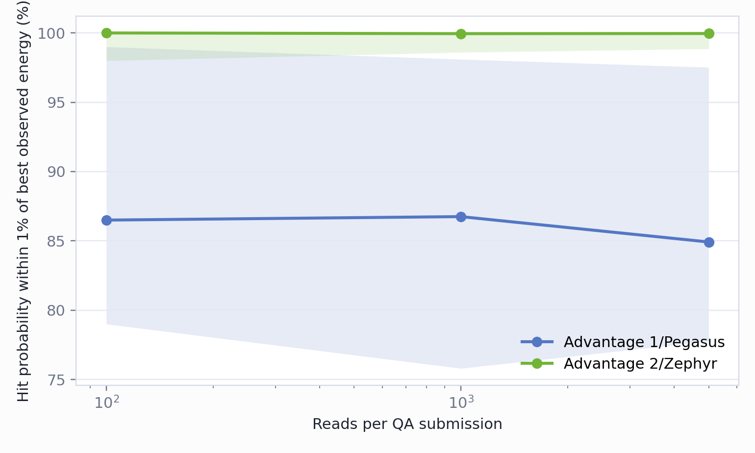
Figure 5: Measured QA hit probability versus reads for a 1% energy-gap target at a 20 \(\mu\)s anneal. The bands show the interquartile range across QUBO size/degree groups..
2.4pt max width=
2.2pt max width=
14 Scheduling Policy Details↩︎
Let \(q\) be a ready stage, \(r(q)\) its target resource, \(s(q)\) its predicted service time, \(a(q)\) its age, \(b(r)\) the backlog for resource \(r\), and \(u(r)\) the current utilization estimate. First-In, First-Out (FIFO) orders stages by arrival time. The other policies assign scores and select the candidate with highest score, subject to resource availability and dependency constraints.
This block expands Section 4.5.3. The main text treats policies as HCU configuration knobs. The appendix records the policy-visible state and scoring intuition needed to interpret the full policy matrix in Appendix 17.4.
Table ¿tbl:tab:policy95state95app? spells out the policy names and records what each policy is allowed to see at dispatch time. This prevents the main policy result from reading like a black box: the performance differences later in the appendix can be traced back to age, queue, bottleneck, and pressure signals.
max width=
14.0.0.1 Hybrid Overhead-Balanced Adaptive (HOBA).
HOBA is the queue-aware dispatch and batching policy used in the paper suite. It gives extra priority to stages that feed under-supplied QA or DQC paths and forms bounded QA/DQC controller batches so setup overhead is amortized without turning one controller into an unbounded serialized queue.
14.0.0.2 Greedy Max Pressure (GMP) and Max-Pressure.
Pressure policies prioritize work that relieves downstream bottlenecks. A generic pressure score is \[S_{\mathrm{pressure}}(q)=P_{\mathrm{down}}(q)-P_{\mathrm{up}}(q)-\lambda s(q),\] where downstream and upstream pressure terms are derived from queue backlog, resource utilization, and dependency structure. GMP uses a greedy pressure score. Max-Pressure emphasizes local queue/backlog differences.
14.0.0.3 Adaptive Batch-Optimal (ABO).
ABO is the arrival-rate-aware batching policy. For a controller setup overhead \(O\), estimated arrival rate \(\lambda\), waiting weight \(W\), and candidate batch size \(b\), the simulator selects the feasible batch size that minimizes \[J(b)=\frac{O}{b}+W\frac{b-1}{2\lambda},\] subject to the QA/DQC batch caps and hard timeout settings. The risk is over-batching when the arrival-rate estimate becomes stale relative to the current workload mix.
All policies use deterministic tie-breaking in the simulator so that repeated runs are comparable. The main text reports policy effects. This appendix records the scoring intuition and equations used to interpret those results.
15 Hardware Validation Grids↩︎
This appendix section records the hardware campaigns behind the compact validation table in the main text. The goal is auditability: a reader should be able to see which backend families, workload-shaped rows, circuit sizes, QUBO sizes, shot/read counts, and timing fields were used to ground the runtime profiles. We therefore separate IBM circuit grid coverage (Table ¿tbl:tab:ibm95grid95app?) and D-Wave QUBO coverage summaries from workload-shaped validation rows (Tables ¿tbl:tab:dwave95workload95rows95app? and ¿tbl:tab:ibm95workload95rows95app?). This section is the detailed evidence for Section 4.4 and the hardware-grounding claim summarized in the main-text validation anchors.
15.0.0.1 IBM circuits.
The IBM calibration and backend-transfer grids vary backend, circuit family, qubit count, logical depth, transpiled depth, shot count, gate counts, optimization/transpilation settings, and measured IBM-reported quantum seconds. Kingston provides the strongest current profile. Marrakesh and Fez provide additional backend-transfer evidence. Workload-shaped rows include portfolio, VQE, pipeline/SQC-style, PES scan, and related DQC circuits.
max width=
15.0.0.2 D-Wave QUBOs.
The D-Wave grids vary target backend, variable count, quadratic terms, density/degree, reads, embedding outcome, chain/embedding metadata, sample-set metadata, QPU access time, programming/readout/sampling fields, and wall time. Workload-shaped rows include bin-packing, vehicle-routing, portfolio, unit-commitment, pipeline/SQC-style, and related optimization instances.
The D-Wave evidence should be read in two layers. The broad runtime grid covers both Advantage 1/Pegasus and Advantage 2/Zephyr over 64–4096 variables, degrees 2, 4, and 6, 100/1000/5000 reads, and 20/100 \(\mu\)s anneals. The training corpus retains 249 Advantage 1 rows and 263 Advantage 2 rows, including 39 and 28 no-embedding observations, respectively. The workload-validation campaign adds 10 successful rows per backend at 12–256 variables, 11–32640 quadratic terms, 1000 reads, and 20 \(\mu\)s anneals. Follow-up D-Wave campaigns add 35 portfolio-variant rows using 107 QPU chunks and 107,000 returned samples, 30 chain-strength rows over strengths default, 0.5, 1.0, 1.5, and 2.0, and 32 four-gauge spin-reversal rows. Table ¿tbl:tab:dwave95workload95rows95app? then gives the application-shaped QUBOs generated by the workload pipeline. Rows that fail to embed are not discarded. They are retained as capacity and feasibility evidence because the simulator optionally uses embedding feasibility as a validation filter.
max width=
max width=
16 Runtime Model Fits↩︎
The QA model predicts physical QPU access time from instance structure, sampling parameters, backend, and embedding-related features. The DQC model predicts IBM-reported quantum seconds from backend, circuit family, qubits, shots, depth, transpiled depth, and gate counts. Cloud wall time is not folded into physical occupancy. It is modeled separately as a deployment overhead mode. This section supports the compact validation anchors in Table 3. It also explains why the main text treats cloud overhead as a deployment mode instead of a device constant.
The main text reports representative fit quality. Full analysis rows retain backend, split, number of observations, absolute error, percentage error, coefficient of determination, and residual summaries.
Tables ¿tbl:tab:backend95fit95details95app?–¿tbl:tab:dwave95timing95decomposition95app? explain how profile grounding is separated into model quality, fitted coefficients, embedding feasibility, and timing decomposition. The most important distinction is that QPU access time and IBM-reported quantum seconds are used as physical occupancy targets, while wall time and provider overhead are retained separately for cloud-proxy experiments. This is the numerical basis for the paper’s claim that cloud execution should not be treated as a device constant.
Table ¿tbl:tab:runtime95coefficients95app? is the audit table for the compact runtime equations in Appendix 9. It is retained as a table, rather than compressed into prose, because reviewers need to see which backend-specific coefficients drive the simulator profiles.
| Target | Predictors and simulator use |
|---|---|
| QA QPU access | Predictors: backend, variables, couplers, reads, timing fields, and embedding metadata. Use: physical QA occupancy. |
| QA cloud wall | Predictors: QPU access plus provider/client overhead fields. Use: optional cloud-proxy mode. |
| DQC quantum seconds | Predictors: backend, circuit family, circuit count, shots, qubits, logical depth, transpiled depth, and gate counts. Use: physical DQC service. |
| DQC cloud wall | Predictors: Runtime job metadata and queue/provider fields. Use: optional cloud-proxy mode. |
| Feasibility | Predictors: qubit footprint, density/degree, capacity, embedding status, and backend limits. Use: optional validation filter. |
max width=
max width=
max width=
Table ¿tbl:tab:dwave95embedding95summary95app? should be interpreted as feasibility evidence, not just as timing data. The embedded rows ground QPU access-time fits. The no-embedding rows explain when the simulator should mark a QA workload as capacity-limited or require a decomposition/alternative backend.
max width=
17 Additional Evaluation Material↩︎
The supplementary evaluation material is organized by the same questions used in Section 5. V2 answers the cloud-versus-integrated execution question. E3 records the mixed-workload stress evidence. S1 expands workload-scaling and capacity-boundary rows, and E5 collects sensitivity and extension analyses that would crowd the main narrative.
This section is the numerical backstop for Section [sec:results]. Every compact main-text result has a dense appendix table with enough state to check the claim: workload, topology, policy, execution mode, runtime, utilization, average queue diagnostics, bottleneck, and capacity status.
Dense tables are retained only when row-level variation is needed for auditability. Repeated patterns with little per-row information are summarized in prose.
17.1 E1/E2/S1: Mechanism Figures for Main-Text Results↩︎
The main text keeps the broad topology payoff, policy frontier, and future compromise plot. This appendix subsection retains the mechanism figures that support those main-text claims but would crowd the 12-page body: controller-pair numerical summaries, DQC bottleneck migration, replica bottleneck movement, policy CPF decomposition, and future bottleneck migration.
17.1.0.1 Topology mechanism behind replica scaling.
The main text reports that adding QPU replicas alone is often insufficient. Figures 6 and 7 provide the supporting mechanism. The CPF-labeled curves use the implementation diagnostic defined in Section 5. A high controller CPF means that controller resources are active for a larger share of the run, exposing a control bottleneck even when additional QPU capacity is available. In the DQC sweep, completion time improves as DQC capacity increases, but controller CPF rises, showing that the next serialized component is often the controller path.
17.1.0.2 Controller-pair numerical summary behind the topology result.
The main text summarizes the pair sweeps numerically: QA-controller replication increases average throughput from 2.85 to 9.75 jobs/s (3.43\(\times\)), while DQC-controller replication reduces p95 completion time from 7601 s to 6348 s (16.5%). The important point is not the full matrix shape but the split in objectives: QA-controller replication is the throughput lever, while DQC-controller replication is the tail-latency lever. We therefore retain the numerical takeaway here and omit the dense heatmap panels from the appendix body.
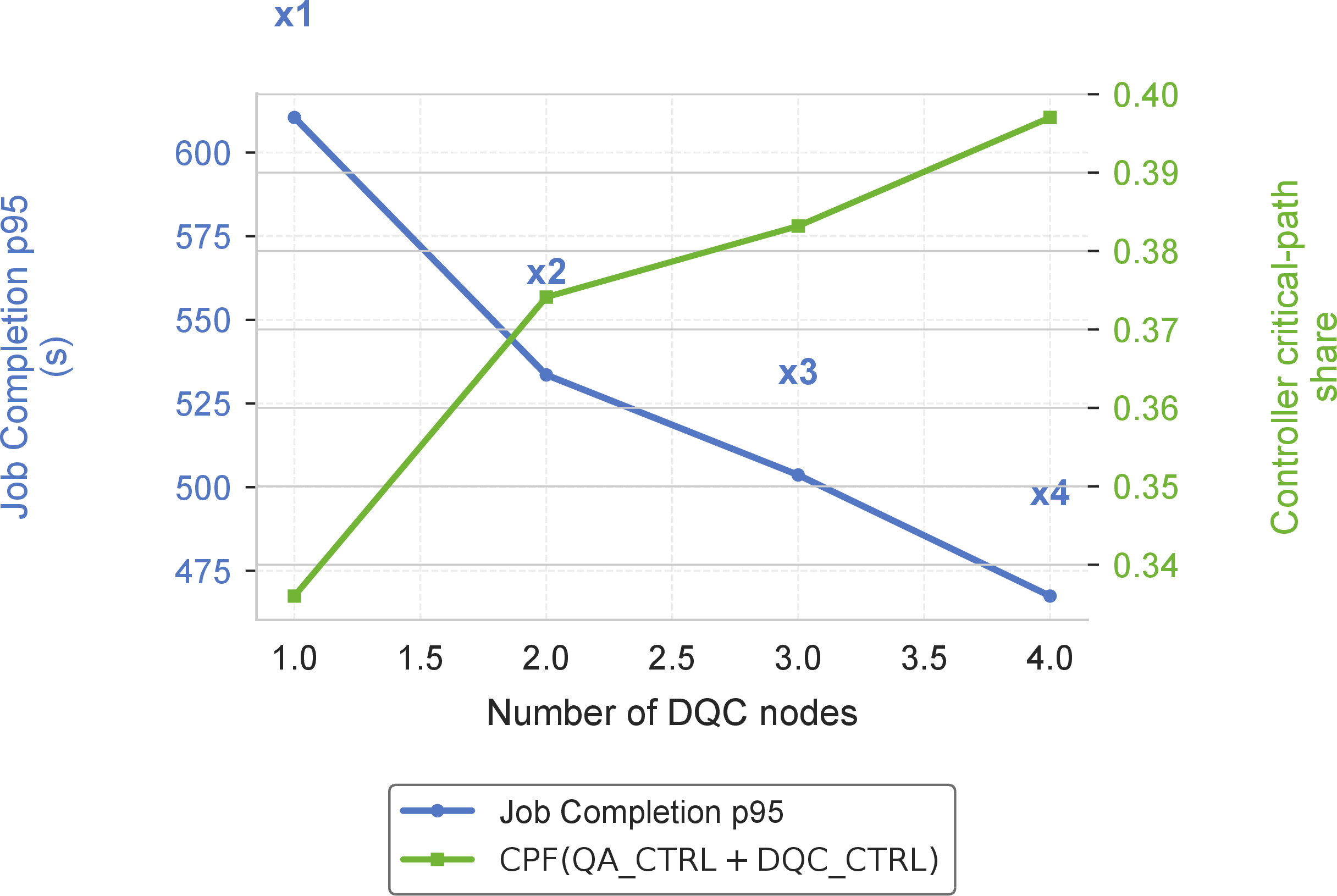

17.1.0.3 Policy decomposition behind the policy frontier.
Figure [fig:e195policy95tradeoff95main] in the main text shows the policy frontier. Figure 8 explains the mechanism behind that frontier: different policies shift active-wall bottleneck pressure across QA, DQC, controller, transfer, and classical components rather than merely changing a single queue order. This supports the main-text claim that scheduling is part of topology co-design rather than a separable software choice.
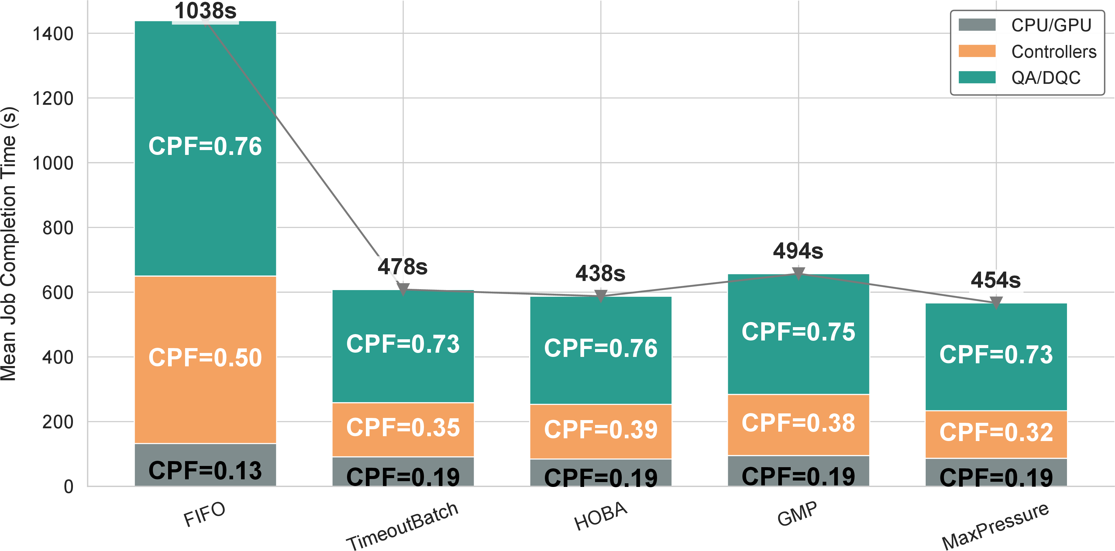
17.1.0.4 Replica and future pair-sweep numerical summaries.
The current-scale replica sweep preserves the same message as the main-text topology result: QA-controller replication is the strongest throughput lever, DQC-controller replication improves p95 completion most, and single-resource QPU replication is not enough when controller paths are already critical. At future scale, the x10 and x100 pair sweeps show the same qualitative behavior with larger residual tail pressure: QA-controller replication continues to move throughput, while p95 completion remains dominated by multi-axis workload growth and does not collapse to the ideal scaling line. We therefore retain these observations as numerical summaries rather than dense heatmap panels.
The tables in this section are intentionally more detailed than the main-text tables. The main text reports the clean claim-level result. The appendix shows the rows needed to audit those claims, including execution mode, scale mode, resource utilization, queue behavior, bottleneck class, and unfinished-job pressure. This lets the reader distinguish three different situations that would otherwise look similar in a plot: a completed run with a long makespan, a completed run with high utilization, and an unfinished run that exposes a capacity or horizon limit.
17.2 V2: Cloud Versus Integrated Execution↩︎
This block answers V2. Applying measured D-Wave wall/access factors to simulated QA service time shows why cloud wall time must remain a deployment knob. Median overhead ratios are near one for DQC-dominated mixed workloads, but QA-only workloads are more sensitive to provider overhead, while DQC-heavy workloads are dominated by DQC service and controller contention. A cloud run can therefore be useful for calibration without being the right model for a local accelerator deployment.
The simulator needs two execution semantics. In cloud-grounded mode, wall time and provider overhead help reproduce today’s end-to-end observations. In tightly integrated mode, physical resource occupancy drives the resource graph. Conflating the two would overstate the cost of local accelerator designs and understate the value of reducing orchestration latency.
Table ¿tbl:tab:cloud95numeric95app? expands the cloud-versus-integrated result. The ratio columns show how much larger the cloud-proxy makespan is than the integrated-HCU makespan, and the delta columns show the absolute seconds added by cloud/provider overhead. QA-only rows are most sensitive to this overhead. DQC-dominated rows are largely governed by DQC service and controller contention. This is why HybridQC models cloud overhead as an execution mode rather than mixing it into physical QPU service.
max width=
17.3 S1: Workload Scaling and Capacity Boundaries↩︎
Figure [fig:future95compromise95speedup95main] in the main text summarizes the compromise point between fixed-HCU and 10\(\times\) larger-HCU execution. The appendix material below provides the numerical rows behind that figure: completed 100\(\times\) representatives, unfinished fixed-HCU capacity-boundary evidence, and the latest scaling matrix.
Table ¿tbl:tab:future95workload95numeric95app? expands the workload-scaling result with representative completed rows under 100\(\times\) scaling. It identifies which resource dominates and whether a larger topology changes that bottleneck. The unfinished fixed-HCU rows are summarized after the table because they all convey the same capacity-boundary pattern rather than a meaningful row-by-row comparison.
max width=
17.3.0.1 Unfinished fixed-HCU capacity-boundary rows.
Under 100\(\times\) all-field scaling on the fixed HCU, four representative rows are DQC-saturated rather than merely slower: cloud scheduling completes 28/30 jobs in \(44.65\times 10^6\) s, pipeline completes 15/30 in \(60.44\times 10^6\) s, transmission switching completes 13/30 in \(83.15\times 10^6\) s, and unit commitment completes 17/30 in \(29.52\times 10^6\) s. All four report DQC utilization of 1.000 under the 400 GB memory configuration. VQE is more severe: it completes 0/30 jobs under the fixed-HCU limits. These rows are architecture warnings under the configured resource constraints, not normal completed-runtime comparisons.
The latest Rust scaling batch adds a second view of workload growth: instead of separating individual scaling axes, it groups completed rows by execution modality and compares current workloads with 10\(\times\) and 100\(\times\) workloads on a larger HCU. Table ¿tbl:tab:latest95hcu95scaling95app? is intentionally grouped by execution type because the central architecture question is whether QA-only, DQC-only, and coupled QA+DQC workloads scale in the same way. They do not: QA-only rows grow roughly with the scale factor, while DQC-heavy rows grow by orders of magnitude because circuit count, depth, shots, controller service, transfers, reconstruction, and queueing interact.
max width=
The fixed-HCU stress runs are capacity-boundary evidence rather than completed runtime ratios. In the broad-suite horizon-limited run, the 10\(\times\) workload on the fixed HCU completes 162 of 594 rows, leaves 48 partial rows, and records 384 zero-completion rows. The 100\(\times\) fixed-HCU run completes 0 of 594 rows. The no-stop follow-up confirms that this is not just a short horizon artifact: at 10\(\times\), QA-only rows complete broadly (108/108 rows, median 22.74 s, p95 33.28 s), but DQC-only rows complete only 18/162 rows with median completed time 59,808 s and p95 120,482 s. Mixed QA+DQC rows complete 36/324 rows with 48 partial rows, median completed time 99,372 s, and p95 257,035 s. At 100\(\times\), the fixed HCU still records no completed broad-suite rows. This distinction is important for the paper’s tone: an unfinished row is not a bad datapoint. It is the simulator telling us that a topology has stopped scaling for that workload family.
17.4 E3: Mixed-Workload Stress and Policy/Topology State↩︎
This block answers E3. Homogeneous experiments are useful for fitting and for clean scaling curves, but mixed workloads reveal the interaction that matters for shared systems. When portfolio, PES scan, VQE, pipeline, and other workloads are co-scheduled, the bottleneck can move from QA to DQC to controllers or transfer links as the job mix changes. The 20-job mixed case is especially revealing: policy changes the makespan by up to 1.80\(\times\), while balanced hardware scaling still leaves significant serialized work.
A future HCU should not be evaluated only on a single benchmark family. A topology that looks over-provisioned for a QA-heavy workload can become under-provisioned when DQC-heavy and transfer-heavy jobs are added. HybridQC makes this visible by preserving the workload graph and resource queues instead of collapsing each job into one quantum-service number.
The full policy and topology matrices are more useful as compact takeaways than as two dense appendix tables. The policy sweep shows three distinct regimes. For bin packing, all policies finish in less than a second because the workload is QA/controller limited. GMP is the fastest at 0.615 s and 16.265 jobs/s, while FIFO is only slightly slower at 0.732 s. For portfolio, the DQC path dominates under every policy: HOBA is best at 66.324 s and 0.151 jobs/s, while ABO and Max-Pressure both stretch to about 75.9 s as the average DQC queue rises to roughly three jobs. For PES scan, policy choice is larger: Max-Pressure finishes in 1223.917 s, while FIFO takes 2403.988 s. The mixed bundle exposes the main scheduling result. FIFO takes 3534.492 s, while HOBA, GMP, and Max-Pressure reduce runtime to 2685.251 s, 2718.180 s, and 2620.508 s respectively. The corresponding DQC queue remains large (11.07–13.38 jobs), so the policy improvement comes from ordering work around the real bottleneck rather than eliminating the bottleneck.
The topology ablation has the same pattern: single-resource upgrades help only when they target the active resource path, while balanced scaling helps every representative workload but remains sublinear. Bin packing is QA/controller-limited, so DQC-only, QA-only, and faster-link-only variants stay at the 0.630 s baseline, while controller replication improves runtime to 0.326 s and balanced 10\(\times\) scaling reaches 0.225 s (2.80\(\times\)). Portfolio is DQC-limited: DQC-only scaling improves runtime from 66.324 s to 37.470 s, while QA-only and faster-link-only variants do not move the result. Balanced scaling reaches 26.857 s (2.47\(\times\)). PES scan is controller/DQC limited: controller-only scaling reduces runtime from 1418.809 s to 1009.149 s, CPU/GPU-only scaling reaches 1253.000 s, and balanced scaling reaches 414.434 s (3.42\(\times\)). In the mixed bundle, DQC-only scaling improves runtime from 2685.251 s to 1778.419 s, CPU/GPU-only to 2215.000 s, and balanced 10\(\times\) scaling to 1226.074 s (2.19\(\times\)). These retained numbers preserve the audit trail for the main claim without spending two full-width tables on rows whose qualitative pattern is repeated.
17.5 E4/E5: Sensitivity and Extension Analyses↩︎
This block answers E4 and E5. Controller/link choices should be evaluated with targeted workload regimes, not only aggregate mixes. An aggregate suite can average away a pathology that dominates a specific workload class. HybridQC keeps controller and link paths explicit so the evaluation can report both the average case and the case that exposes the architectural risk.
The targeted controller/link sweeps are useful as sensitivity evidence at current scale but become capacity probes on the fixed HCU at future scale. At 1\(\times\), VQE and PES scan complete across communication-link/jitter, cross-fabric control, and controller/QPU-link/replica sweeps: PES scan finishes 240/240 link rows, 90/115 cross-fabric rows, and 240/240 controller/link rows, with median runtimes of 3440.0–3665.3 s. VQE finishes the same row groups with median runtimes of 3320.1–3343.3 s. At 10\(\times\) on the fixed HCU, PES scan reaches no completed jobs, while VQE reaches a median of four completed jobs out of fifty in the grouped rows. At 100\(\times\), neither workload progresses to completion. These rows explain why fine-grained link/control differences should be studied only after the base topology can carry the scaled DQC demand.
The larger-HCU targeted sweeps answer the complementary question: once the topology is enlarged enough for the scaled workload to finish, do controller and link variants become measurable? They do. Both 10\(\times\) and 100\(\times\) larger-HCU runs complete 1172 of 1222 rows. At 10\(\times\), PES scan has median runtime near 38,750 s across link/jitter, control-fabric, controller/link, and graph-search sweeps, while VQE has median runtime near 260,935 s. At 100\(\times\), PES scan is already in the million-second range, with median runtime near 5.44M s and median DQC utilization about 0.926–0.927. VQE reaches about 208.88M s with median DQC utilization about 0.544. These rows therefore support the result that workload-scale sensitivity studies need sufficient base capacity before fine-grained controller/link variants become interpretable.
The QA load-amplification simulator-integration sweep integrates the D-Wave-grounded QA success curve into full HCU execution. At 1\(\times\) current scale, load shedding changes the median runtime from 156.4 s at a 1\(\times\) relative cap to 7.43 s at 8\(\times\) and 5.30 s at 16\(\times\). Throughput rises from 0.192 to 4.04 and then 6.17 jobs/s. The quality-fixed mode shows why the load-shedding decision is needed: blindly scaling QA effort to 4\(\times\) worsens median runtime from 151.8 s to 167.5 s, while 16\(\times\) improves it to 19.84 s only after enough DQC fallback pressure is removed. At future scales, the rows are largely DQC-bound: 10\(\times\) larger-HCU load-shedding rows remain at 66,743 s across caps, and 100\(\times\) larger-HCU load-shedding rows remain at 56.99M s. This distinction prevents overclaiming the QA result: hardware SampleSets ground the quality curve, while the simulator identifies when that curve is actually on the HCU critical path.
The broader architecture-search evidence is retained as a numerical interpretation rather than a final floating figure. It shows the same tradeoff as the targeted topology results in Section [sec:results]: improving one resource class can move the bottleneck instead of removing it, so useful topology search must reason jointly about makespan, utilization, controller capacity, and resource balance.