Adapting Generalist Vehicle Models for
High-Speed MPC Across Terrains
July 14, 2026
Abstract
High-speed off-road autonomy requires precise closed-loop control for a target vehicle while remaining robust across changing terrains. Recent forward kinodynamic (FKD) prediction foundation models suggest a promising path, starting from a generalist
model and specializing it to the target platform. However, effective specialization remains challenging, as it often requires substantial real-world data, and models adapted to one setting can still overfit to specific terrains or driving regimes. We
present OptCar (Optimized Car), a recipe for bridging the gap from generalist to specialist FKD models that preserves cross-terrain generalization while optimizing performance for a specific vehicle. OptCar introduces a
history-conditioned dynamics adaptation module that encodes recent state-action observations into a dynamics context token, and then fine-tunes the generalist model using limited real-world data together with targeted synthetic rollouts from
environment-specific system identification. In closed-loop model predictive control (MPC) experiments across three terrains and an out-of-distribution cart-pulling task, the largest gains appear at 6 m/s, the highest speed evaluated and the regime in which
slip dominates tracking error. On vegetation and dirt, the most slip-diverse terrain, OptCar reduces 6 m/s trajectory tracking error by roughly 55% relative to a fine-tuned AnyCar baseline, and remains the most accurate even when an unseen
cart payload changes the dynamics. With only 5 minutes of real data per terrain, OptCar is competitive on road with a specialist trained on 30 minutes of road data, and substantially outperforms it once the terrain changes.
1 Introduction↩︎
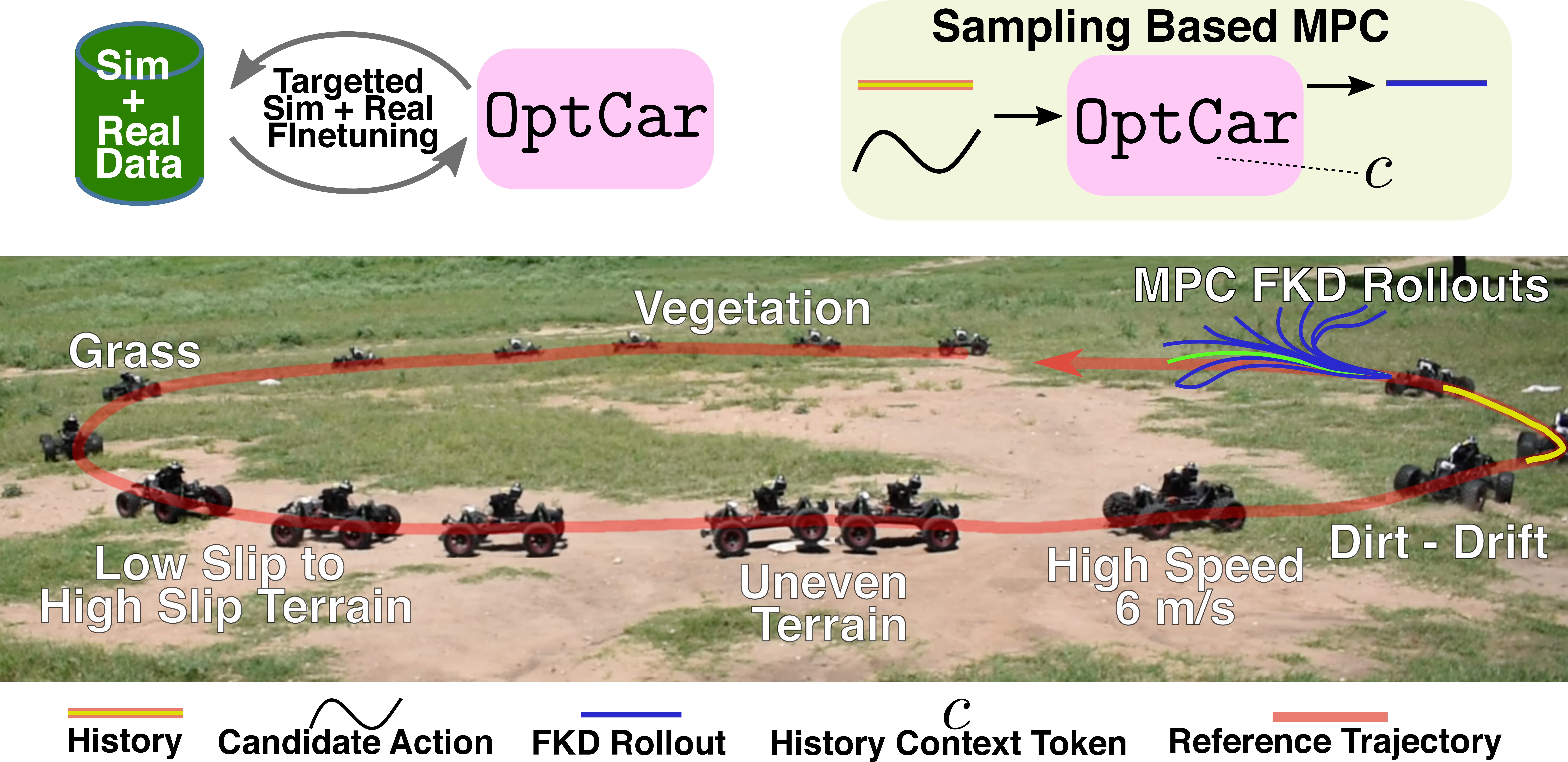
High-speed driving over unstructured terrain underlies applications from search-and-rescue and agricultural robotics to autonomous off-road racing. It is hard because at high speed the tires operate near their friction limit, and the resulting slip varies with terrain and payload, so a controller must be both precise on the target vehicle and robust as the terrain changes. Analytical models such as the dynamic bicycle model are fast but break down in this high-slip regime; learned models capture it, but to run in real time on embedded hardware at high speed the model must be small, so accuracy must come under a tight fidelity-latency budget rather than from a larger network.
Forward kinodynamic (FKD) models predict future states from candidate action sequences and serve directly as the rollout model inside sampling-based model predictive control (MPC), such as MPPI [1], coupling planning and control. Generalist FKD models such as AnyCar [2] generalize across vehicles and environments but lack the per-vehicle accuracy needed for high-speed control, whereas inverse kinodynamic (IKD) methods [3], [4] adapt online to the current terrain through an explicit history component but rely on a separate planner. At the other extreme, specialist models fit a single vehicle and terrain from extensive real data [5], [6], achieving aggressive performance in that setting but not transferring elsewhere. Specializing a generalist FKD model to a known vehicle while remaining robust across terrains is the central problem we address.
We present OptCar (Figure 1), which addresses these limitations and is validated by placing the model inside an MPPI controller [1] for closed-loop trajectory tracking. Its contributions are:
A history-conditioned FKD architecture that compresses recent state-action history into a single dynamics context vector and conditions every block of the rollout decoder on it. Adding this conditioning lowers 6 m/s tracking error by 21% to 33% across terrains relative to the same backbone without it.
A targeted real-and-synthetic fine-tuning recipe that specializes the model to a target vehicle from only minutes of real data per terrain, augmenting it with synthetic rollouts from a per-terrain system-identified bicycle model to cover the high-slip regimes. This lowers 6 m/s tracking error by a further 17% to 46% over fine-tuning on real data alone.
Closed-loop validation against generalist and specialist models. Against the generalist AnyCar baseline,
OptCarfine-tuned on real and synthetic data cuts 6 m/s tracking error by 42% to 57%. Against a specialist trained on 30 minutes of road data, it remains within 14% on road yet tracks 46% more accurately on unseen terrain. Under an unseen cart payload, it attains the lowest tracking error at every speed regime.
2 Related Work↩︎
In this section, we review related work in terms of learned dynamics models for vehicle control, online dynamics adaptation, and data-efficient specialization via sim-to-real.
2.1 Learned Dynamics Models for Vehicle Control↩︎
We frame high-speed vehicle control as model-based planning under dynamics that vary with vehicle, terrain, and payload. Analytical kinematic and dynamic bicycle models [7] are fast and interpretable but break down under aggressive tire-terrain interaction, while end-to-end policies [8] forgo the predictive rollouts needed to evaluate alternative futures. Learned forward kinodynamic (FKD) models occupy the middle ground we adopt, predicting future trajectories from candidate actions and serving as rollout models inside sampling-based MPC [1], [5], [9]. Within FKD-MPC, generalist models such as AnyCar [2] are trained across many vehicles and environments for broad transfer, whereas specialist methods fit models to a single vehicle, terrain, or regime using extensive real data: drifting and tire models [6], off-road and terrain-aware rollouts [10], [11], and information-theoretic or residual-dynamics racing controllers [5], [12]–[14], none of which transfer across terrains. Our setting lies between the two, with a fixed vehicle that makes specialization worthwhile and a varying terrain that makes single-terrain specialization insufficient.
2.2 Online Dynamics Adaptation↩︎
Online adaptation methods infer the active dynamics from recent experience, using state-action histories to condition policies [15], [16], represent changing disturbances [17], [18], or perform terrain-adaptive ground-vehicle tracking [3], [4]. For learned dynamics models, prior work adapts through online parameter updates [19], [20] or latent context for one-step probabilistic MPPI rollouts [21]. OptCar instead adapts in a single forward pass: a history-conditioned context vector modulates a
multi-step FKD rollout decoder, so adaptation requires no online optimization and directly shapes the candidate-action rollouts MPC evaluates.
2.3 Data-Efficient Specialization and Sim-to-Real↩︎
OptCar’s second contribution, a targeted real-and-synthetic fine-tuning recipe, relates to the sim-to-real literature that uses limited real data to calibrate simulators or domain-randomization distributions [22]–[26]. These methods typically calibrate a simulator and then train a model or deploy a controller within it, or tune a global randomization distribution. OptCar instead uses a per-terrain calibrated dynamic
bicycle model purely as a targeted data generator that augments scarce real data with samples from high-slip regimes that the real data undersample; the learned FKD model, not the calibrated simulator, remains the rollout model deployed in MPC. This
approach anchors the synthetic data to the target vehicle instead of distributing them across a broad randomization distribution.
3 Problem Formulation↩︎
We consider forward kinodynamic (FKD) prediction for a target vehicle: given a history of recent states and applied actions together with a candidate future action sequence, the goal is to predict the resulting future state trajectory. Let \(\mathbf{s}_t \in \mathcal{S}\) denote the vehicle state (pose and velocity) at time \(t\) and \(\mathbf{a}_t \in \mathcal{A}\) the applied action (body-frame velocity and steering command). Given a history length \(M\) and prediction horizon \(N\), we seek a deterministic prediction model \(f_\theta\) that maps the recent history and a candidate future action sequence to the predicted future trajectory, \[\hat{\mathbf{s}}_{t+1:t+N} = f_\theta\!\left(\mathbf{s}_{t-M:t},\; \mathbf{a}_{t-M:t+N-1}\right), \label{eq:fkd}\tag{1}\] with parameters \(\theta\) chosen to minimize prediction error over the predicted future states \(\hat{\mathbf{s}}_{t+1:t+N}\) on the operational distribution of the target vehicle across its terrains. Because it runs in closed-loop control, the model must be small enough to roll out many candidate actions in real time.
4 Methodology↩︎
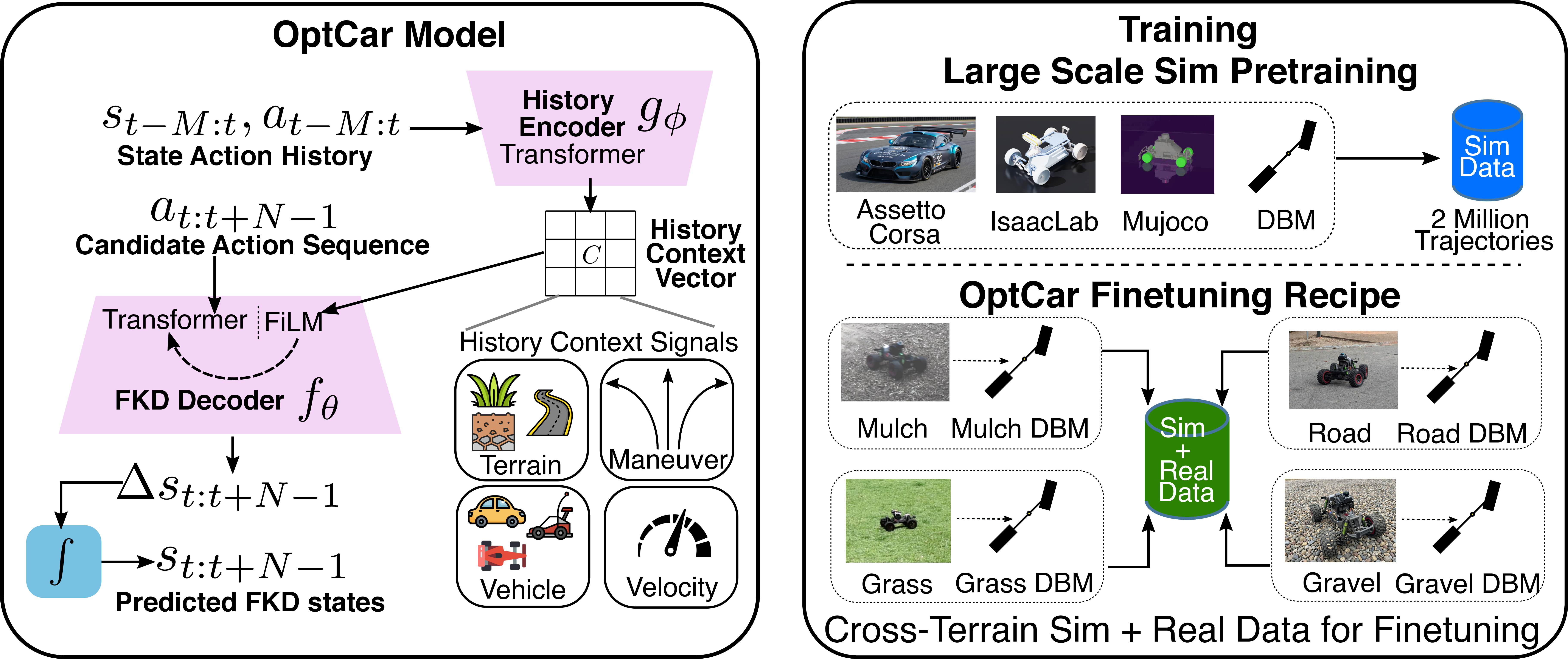
OptCar specializes a pretrained FKD model to a target vehicle while adapting across terrains (Figure 2). The approach is built around two ideas. First, the changing vehicle-terrain interaction is treated
as a latent dynamics condition inferred online from recent motion; this inferred context then conditions all candidate future rollouts evaluated by MPC. Second, target-vehicle specialization is performed with limited real data augmented by targeted
synthetic rollouts from terrain-specific system identification, expanding coverage of high-slip regimes that are difficult to collect safely.
4.1 History-Conditioned FKD Prediction↩︎
At high speed, the future motion of the vehicle is not determined by the measured state and commanded action alone. The same action sequence can produce different rollouts depending on latent factors such as terrain friction, slip regime, payload, and
actuator response. These factors are not directly observed by the controller, but recent state-action transitions provide a local system-identification signal. OptCar therefore realizes the predictor of Eq. 1 in two
stages: a history-to-context map \(g_\phi\) and a context-conditioned rollout map \(f_\theta\) whose predicted increments integrate to the future trajectory:
\[\mathbf{c}_t = \underbrace{g_\phi\!\left(\mathbf{s}_{t-M:t-1},\; \mathbf{a}_{t-M:t-1}\right)}_{\text{history-to-context map}}; \quad \Delta\hat{\mathbf{s}}_{t+1:t+N} =
\underbrace{f_\theta\!\left(\mathbf{s}_t,\; \mathbf{a}_{t:t+N-1},\; \mathbf{c}_t\right)}_{\text{context-conditioned rollout map}}. \label{eq:factorization}\tag{2}\] The context \(\mathbf{c}_t \in
\mathbb{R}^d\) is not supervised with terrain or regime labels; it is learned end-to-end as the information from recent motion that is useful for predicting future rollouts. This factorization creates a bottleneck between history processing and
rollout prediction: all history-dependent information available to the rollout model must pass through \(\mathbf{c}_t\). Rather than letting the decoder optionally attend to history tokens, OptCar conditions
every block of the rollout map \(f_\theta\) on \(\mathbf{c}_t\): \[\mathbf{h}^{(l+1)} =
\mathcal{B}^{(l)}_\theta\!\left(\mathbf{h}^{(l)};\, \mathbf{c}_t\right), \qquad l = 1,\dots,L, \label{eq:block95conditioning}\tag{3}\] where \(\mathcal{B}^{(l)}_\theta\) is the \(l\)-th block of the rollout map \(f_\theta\) and \(\mathbf{h}^{(l)}\) its hidden representation, with conditioning realized by FiLM [27] in our implementation. Every candidate rollout for the sampling-based MPC is conditioned on the same dynamics context,
and \(\mathbf{c}_t\) is computed once per planning step and reused across all candidate action sequences.
The decoder predicts body-frame pose increments \(\Delta\hat{\mathbf{s}}_{t+k} = (\Delta\hat{\mathbf{p}}_{t+k}, \Delta\hat{\mathbf{q}}_{t+k})\) rather than global poses. This local representation removes dependence on global position and supports rollouts over non-planar terrain. Architecture and training details are summarized in Section 5, with exact conditioning and integration equations in Appendix 8.
4.2 Pretraining as a Generalist FKD Prior↩︎
Before target-vehicle specialization, OptCar is pretrained on a large simulation corpus spanning diverse vehicles, terrains, and driving regimes. The purpose of pretraining is to learn a broad prior over action-conditioned vehicle motion
and to learn how recent state-action history can identify the active dynamics. Both the history-to-context map \(g_\phi\) and the rollout map \(f_\theta\) are trained jointly from random
initialization. The training target is the body-frame future increment sequence in Eq. 2 ; corpus and loss details are summarized in Section 5 and Appendix 8.
4.3 Targeted Real-and-Synthetic Specialization↩︎
Fine-tuning must balance relevance and coverage. Real target-vehicle data are most relevant but sparse in the aggressive high-slip regimes that matter for MPC, while broad simulation randomization adds coverage at the cost of capacity spent on unrelated
vehicles and terrains. OptCar instead uses each per-terrain real dataset twice, as direct training data and as the calibration signal for a terrain-specific synthetic data generator anchored to the same vehicle.
Let \(\mathcal{D}^e_{\text{real}}\) denote the real target-vehicle trajectories collected on terrain \(e \in \mathcal{E}\). For each terrain, we identify the parameters \(\psi_e\) of a dynamic bicycle model (DBM) \(F_{\psi_e}\) by fitting one-step transitions: \[\psi_e^* = \arg\min_{\psi_e} \sum_{(\mathbf{s}_t,\mathbf{a}_t,\mathbf{s}_{t+1}) \in \mathcal{D}^e_{\text{real}}} \left\| F_{\psi_e}(\mathbf{s}_t,\mathbf{a}_t) - \mathbf{s}_{t+1} \right\|^2. \label{eq:sysid}\tag{4}\] The calibrated model \(F_{\psi_e^*}\) is not deployed as the controller’s rollout model. Instead, it is used offline to generate targeted synthetic rollouts \(\mathcal{D}^e_{\text{synth}}\) under randomized action sequences. These rollouts enter high-slip regions undersampled by the real data while remaining tied to the identified vehicle-terrain dynamics. The final fine-tuning set is \[\mathcal{D}_{\text{FT}} = \bigcup_{e \in \mathcal{E}} \left(\mathcal{D}^e_{\text{real}} \cup \mathcal{D}^e_{\text{synth}}\right), \label{eq:ft95dataset}\tag{5}\] and the pretrained model is fine-tuned end-to-end on \(\mathcal{D}_{\text{FT}}\) with the same pretraining prediction loss.
4.4 Deployment in Sampling-Based MPC↩︎
The fine-tuned model is the rollout function inside an MPPI controller [1]. At each planning step, the history window is encoded into \(\mathbf{c}_t\), candidate actions are rolled out with \(f_\theta(\cdot,\cdot,\mathbf{c}_t)\), and the first action of the lowest-cost sequence is applied. Since adaptation occurs through the forward pass that computes \(\mathbf{c}_t\), deployment needs no terrain classifier, mode switch, or online parameter update.
5 Implementation Details↩︎
5.0.0.1 Architecture.
OptCar uses the transformer FKD backbone and simulation protocol of AnyCar [2], with history processing factored as in Eq. 2 . State, action, command, and current-state inputs are embedded by per-stream MLPs into a shared dimension \(d=64\). The history encoder is a 2-layer bidirectional transformer that maps
\(M=250\) history steps at \(\Delta t=0.02\) s to the context vector \(\mathbf{c}_t\). The rollout decoder is a 2-block causal transformer with 4 attention
heads and feed-forward dimension 256, conditioned by \(\mathbf{c}_t\) through FiLM at each block, and predicts \(N=50\) body-frame SE(3) increments. Appendix 8 gives the conditioning equations and body-frame integration.
5.0.0.2 Training.
We pretrain on approximately 2 million simulated trajectories from the AnyCar protocol across Assetto Corsa, MuJoCo, Isaac Lab, and randomized analytical dynamic bicycle models. The objective is \(\mathcal{L}=1.0\,\mathcal{L}_{\text{pos}}+0.3\,\mathcal{L}_{\text{quat}}\) (Appendix 8); optimization uses AdamW with weight decay \(10^{-2}\), learning rate \(10^{-3}\), cosine annealing, linear warmup, 500 epochs, and batch size 4096.
Fine-tuning uses approximately 5 minutes of real driving per terrain on road, gravel, grass, and mulch, yielding about 60K real history+future windows. Targeted simulation adds about 400K windows by rolling out each \(F_{\psi_e^*}\) for 10 s at \(\Delta t=0.02\) s under randomized Bézier velocity and random-walk steering commands within \([-2,8]\) m/s and \([-0.41,0.41]\) rad, with velocity noise \(\sigma=0.2\). Fine-tuning uses the same optimizer for 200 epochs at learning rate \(10^{-3}\).
5.0.0.3 Deployment.
MPPI samples 600 candidate action sequences per step and scores each rollout with \[C = \sum_{t=1}^{H} \gamma^t \left[ w_p \left(e_{\text{long},t}^2 + 15\,e_{\text{lat},t}^2\right) + w_\psi \Delta\psi_t^2 + w_v (v_t - v_{\text{ref}})^2 \right], \label{eq:mppi95cost}\tag{6}\] where \(\gamma=0.97\) and lateral error is weighted \(15\times\) relative to longitudinal error. The system is implemented in PyTorch and CuPy and runs onboard an NVIDIA Jetson AGX Orin.
6 Experiments↩︎
We design experiments to answer three research questions:
Specialized generalist versus baselines: Can
OptCarmatch or exceed both generalist and specialist models in cross-terrain tracking and out-of-distribution dynamics settings?Targeted real-and-synthetic fine-tuning: Does fine-tuning on limited real data combined with targeted synthetic rollouts improve closed-loop tracking over fine-tuning on just real data?
History context encoding: Does the history context encoder improve closed-loop control over an otherwise identical model without it?
6.1 Experimental Setup↩︎

6.1.0.1 Platform setup:
All experiments use our target 1/5-scale off-road vehicle with an onboard 3D LiDAR sensor, an IMU, and an NVIDIA Jetson AGX board (Figure 3). Localization is provided by SuperOdometry [28], and a low-level PD controller maps commanded velocities to PWM signals.
6.1.0.2 Reference trajectories and terrains:
We evaluate closed-loop figure-8 tracking at three commanded speeds: easy (\(v_{\text{ref}} = 2\) m/s), medium (\(v_{\text{ref}} = 4\) m/s), and hard (\(v_{\text{ref}} = 6\) m/s). Road uses a tighter 17 m figure-8, while wet grass on a slope and vegetation+dirt use a 30 m figure-8 so that 6 m/s tracking remains feasible while preserving the high-slip modeling challenge. The trajectory parameterization is given in Appendix 9.
6.1.0.3 Metrics.
We report trajectory tracking error (TTE), the mean distance from the vehicle to the closest point on the reference trajectory, and velocity tracking error (VTE), the mean absolute deviation from the commanded speed.
6.1.0.4 Baselines.
We compare OptCar fine-tuned on real and targeted synthetic data (OptCar FT-RS) against a per-terrain system-identified dynamic bicycle model used directly inside MPC (DBM), AnyCar [2] fine-tuned on real target-vehicle data only (AnyCar FT-R), IKD fine-tuned on real data (IKD FT-R, Appendix 11), OptCar fine-tuned on real target-vehicle data only (OptCar FT-R), and a specialist OptCar model trained only on 30 minutes of real road data
(OptCar Specialist). Here FT denotes fine-tuning, R denotes real data, and S denotes simulated data.
6.2 RQ1: Baseline Comparisons↩︎
We evaluate OptCar against generalist, specialist, and analytical baselines in three settings: cross-terrain figure-8 tracking, an unseen cart-pulling payload, and transfer beyond the road-only specialist’s training environment.
Table ¿tbl:tab:fig8? summarizes the closed-loop tracking results.
ll cc cc cc & & & &
(lr)3-4 (lr)5-6 (lr)7-8 Env. & Method & TTE & VTE & TTE & VTE & TTE & VTE
& DBM & 0.011 & 0.004 & 0.034 & 0.019 & 0.562 & 1.234
& IKD FT-R & 0.016 & 0.032 & 0.067 & 0.189 & 0.412 & 1.849
& AnyCar + FT-R & 0.013 & 0.009 & 0.025 & 0.025 & 0.248 & 0.912
& Specialist & 0.012 & 0.007 & 0.020 & 0.020 & 0.093 & 0.711
& FT-R & 0.018 & 0.004 & 0.034 & 0.027 & 0.196 & 0.911
& + FT-RS & 0.016 & 0.013 & 0.026 & 0.023 & 0.106 & 0.901
& DBM & 0.012 & 0.017 & 0.156 & 0.044 & 1.356 & 1.456
& IKD FT-R & 0.013 & 0.029 & 0.062 & 0.255 & 2.371 & 1.004
& AnyCar + FT-R & 0.011 & 0.025 & 0.100 & 0.083 & 1.082 & 0.892
& Specialist & 0.013 & 0.016 & 0.146 & 0.051 & 1.149 & 1.056
& FT-R & 0.013 & 0.027 & 0.031 & 0.078 & 0.751 & 0.933
& + FT-RS & 0.012 & 0.025 & 0.044 & 0.011 & 0.625 & 0.940
& DBM & 0.061 & 0.041 & 0.276 & 0.312 & 0.824 & 1.118
& IKD FT-R & 0.055 & 0.033 & 0.232 & 0.452 & 0.669 & 1.452
& AnyCar + FT-R & 0.054 & 0.019 & 0.207 & 0.199 & 0.776 & 0.991
& FT-R & 0.055 & 0.020 & 0.171 & 0.172 & 0.519 & 0.981
& + FT-RS & 0.059 & 0.023 & 0.157 & 0.072 & 0.348 & 0.937
& DBM & 0.129 & 0.014 & 0.212 & 0.197 & 1.012 & 1.881
& IKD FT-R & 0.067 & 0.086 & 0.244 & 0.102 & 0.711 & 1.782
& AnyCar + FT-R & 0.042 & 0.031 & 0.182 & 0.049 & 0.489 & 1.338
& + FT-RS & 0.011 & 0.004 & 0.085 & 0.044 & 0.229 & 1.023
6.2.1 Figure-8 Trajectory Tracking in Three Test Environments↩︎
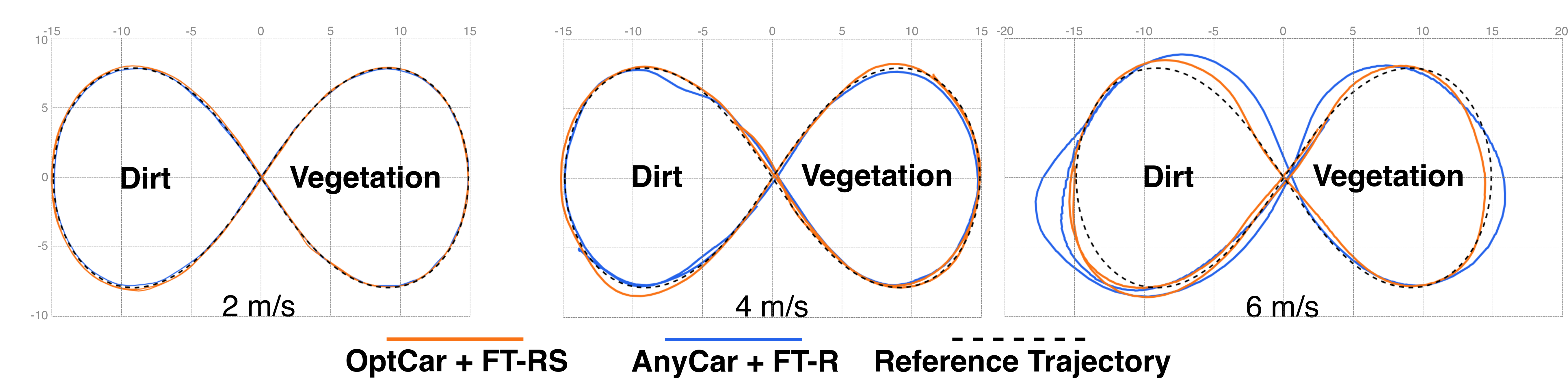
The vehicle executes figure-8 trajectories on road, wet grass on a slope, and vegetation+dirt at 2, 4, and 6 m/s. Each configuration is repeated three times, with each run lasting 15 s, and all models use identical MPPI parameters. Tracking accuracy is
comparable across methods at low slip and diverges as speed and terrain-induced slip increase. At 2 m/s, all methods operate near the nominal regime and perform similarly. At 4 m/s, performance remains close on road, whose high traction keeps the dynamics
predictable, while differences emerge on the lower-traction terrains. The separation is clearest at 6 m/s: OptCar FT-RS attains the lowest trajectory tracking error on every terrain, and on vegetation+dirt its error is less than half that of
AnyCar FT-R (Figure 4). IKD FT-R degrades most under high slip, as it tracks states produced by a separate DBM-MPPI planner rather than scoring candidate actions with the same learned dynamics used for execution.
6.2.2 Out-of-Distribution Cart Pulling↩︎
The cart-pulling task evaluates whether adaptation extends beyond the terrains seen during fine-tuning. The trailing cart alters the vehicle’s effective inertia and tire loading, and no cart data is used during training. OptCar FT-RS
attains the lowest tracking error across all speeds, with the largest margin at 6 m/s (Figure 5). This indicates that the history context does not merely encode the training terrains but infers the unseen dynamics shift from
recent motion.

6.2.3 Comparison Against a Specialist Model↩︎
The road specialist provides a single-terrain reference: it uses the same OptCar architecture but is fine-tuned only on 30 minutes of real road data. On road, the specialist attains the best 6 m/s tracking, and OptCar FT-RS
remains close despite using only 5 minutes of real data per terrain. On wet grass on a slope, the specialist’s accuracy degrades, and the specialist performs substantially worse than OptCar FT-RS. This illustrates the RQ1 tradeoff:
single-terrain specialization is accurate in-distribution but does not transfer, whereas multi-terrain specialization remains accurate when the terrain changes.
6.3 RQ2: Targeted Real-and-Synthetic Fine-Tuning↩︎
To isolate the effect of targeted synthetic data, we compare OptCar FT-R against OptCar FT-RS in Table ¿tbl:tab:fig8?. Both use the same history-conditioned architecture and real target-vehicle data;
OptCar FT-RS additionally trains on synthetic rollouts generated from terrain-specific system identification. The model trained on real and synthetic data is consistently stronger at 6 m/s, where aggressive slip dominates closed-loop error,
while the real-only model remains competitive in moderate regimes. This supports the fine-tuning recipe: real data anchors the model to the target vehicle, while targeted synthetic data fills high-slip state-action regions that are difficult to collect
safely.
6.4 RQ3: History Context Encoding↩︎
To isolate the effect of explicit history context, we compare AnyCar FT-R against OptCar FT-R in Table ¿tbl:tab:fig8?. Both are fine-tuned on the same real target-vehicle data; OptCar FT-R adds the history
context encoder and FiLM-conditioned decoder. The gains are largest at 6 m/s and on lower-traction terrains, where recent state-action transitions are most informative about the active slip regime. The zero-shot cart-pulling result in §6.2.2 reinforces this mechanism: the same encoder helps under an unseen payload shift without cart-specific training data. A more extensive analysis of the learned context vector, projected with PCA and LDA, shows that it
organizes recent history into interpretable dynamics factors such as vehicle, terrain, speed, and turn direction (Appendix 12).
7 Conclusion↩︎
We present OptCar, a recipe for specializing a generalist FKD foundation model to a target vehicle while keeping the model accurate during real-time MPC as the terrain changes. Our experiments yield three lessons. First, a single model can
be both specialized to one vehicle and robust across terrains. Starting from a generalist prior and conditioning it on recent motion makes the model accurate on the target vehicle, while a specialist trained on a single terrain fails once the terrain
changes. Second, history-conditioning provides online adaptation to both terrain and an unseen cart payload, with no separate planner, terrain classifier, or online optimization. Third, targeted synthetic data from per-terrain system identification
resolves the coverage-relevance trade-off of fine-tuning. Together, these components enable OptCar—using only 5 minutes of real data per terrain—to roughly halve 6 m/s tracking error relative to a fine-tuned generalist and remain competitive
with a 30-minute single-terrain specialist on its home terrain while staying accurate elsewhere. More broadly, history-conditioning paired with targeted system-identification data offers a practical path to deploying foundation dynamics models on a
specific robot without collecting large per-terrain datasets.
7.0.0.1 Limitations and future work.
First, OptCar adapts only through its feedforward context vector and never updates its weights online, so it assumes the encountered dynamics lie within the pretraining and fine-tuning distribution. Genuinely novel dynamics would instead
call for online model adaptation, as in meta-learning that updates the dynamics model on the fly [19], and combining fast feedforward context with slower online weight updates is a promising middle ground. Second, real-time MPPI tightly constrains the rollout model. Even with a model of only about 300K parameters, the
controller can afford only a short horizon of \(N=50\), because lengthening it slows each rollout and reduces the number of action samples evaluated per step. This myopic horizon motivates a scaling-law study of the
trade-off between model capacity, rollout horizon, and sample budget. Third, OptCar adapts from proprioceptive history alone, and adding exteroceptive inputs such as RGB images or geometric terrain representations (e.g., point clouds or
elevation maps) could supply richer context and anticipate terrain changes before they appear in recent motion.
8 Architecture and Training Details↩︎
8.0.0.1 Context extraction and FiLM conditioning.
The per-stream history embeddings are concatenated with learned positional encodings to form the history sequence \(\mathbf{M}_t\). The history-to-context map \(g_\phi\) is implemented as a bidirectional transformer encoder with a learnable summary token \(\texttt{[CTX]}\) prepended to the sequence: \[\left[\,\mathbf{c}_t;\; \tilde{\mathbf{M}}_t\,\right] = \operatorname{Enc}_\phi\!\left(\left[\,\texttt{[CTX]};\; \mathbf{M}_t\,\right]\right). \label{eq:ctx}\tag{7}\] Only the summary output \(\mathbf{c}_t\) is passed to the rollout decoder; the refined per-step tokens \(\tilde{\mathbf{M}}_t\) are discarded. Each decoder block is conditioned with Feature-wise Linear Modulation: \[\tilde{\mathbf{D}}^{(l)} = \boldsymbol{\gamma}^{(l)}(\mathbf{c}_t) \odot \mathbf{D}^{(l)} + \boldsymbol{\beta}^{(l)}(\mathbf{c}_t), \label{eq:film95post}\tag{8}\] where \(\mathbf{D}^{(l)}\) denotes decoder features at block \(l\), and \(\boldsymbol{\gamma}^{(l)}, \boldsymbol{\beta}^{(l)} : \mathbb{R}^d \to \mathbb{R}^d\) are learned affine projections. Each decoder block contains two FiLM modules, applied after self-attention and after the full block. The affine projections are initialized so that \(\boldsymbol{\gamma}^{(l)} \approx \mathbf{1}\) and \(\boldsymbol{\beta}^{(l)} \approx \mathbf{0}\).
8.0.0.2 Body-frame rollout integration.
The decoder head outputs body-frame pose increments \(\Delta\hat{\mathbf{s}}_{t+k} = (\Delta\hat{\mathbf{p}}_{t+k}, \Delta\hat{\mathbf{q}}_{t+k})\). The rollout used by MPC is recovered by integrating these increments from the current pose, taken as the local origin \((\hat{\mathbf{p}}_t, \hat{\mathbf{q}}_t) = (\mathbf{0}, \mathbf{q}_{\mathrm{id}})\): \[\hat{\mathbf{q}}_{t+k} = \hat{\mathbf{q}}_{t+k-1} \otimes \Delta\hat{\mathbf{q}}_{t+k}, \qquad \hat{\mathbf{p}}_{t+k} = \hat{\mathbf{p}}_{t+k-1} + \mathbf{R}\!\left(\hat{\mathbf{q}}_{t+k-1}\right) \Delta\hat{\mathbf{p}}_{t+k}, \label{eq:euler}\tag{9}\] for \(k = 1, \dots, N\), where \(\mathbf{R}(\cdot)\) is the rotation matrix of a unit quaternion, \(\otimes\) denotes quaternion multiplication, and \(\mathbf{q}_{\mathrm{id}}\) is the identity quaternion.
8.0.0.3 Training loss.
The pretraining and fine-tuning loss combines position MSE with a geodesic quaternion loss: \[\mathcal{L} = \lambda_p \sum_{k=1}^{N} \left\| \Delta\hat{\mathbf{p}}_{t+k} - \Delta\mathbf{p}_{t+k} \right\|^2 + \lambda_q \sum_{k=1}^{N} d_{\text{geo}}\!\left(\Delta\hat{\mathbf{q}}_{t+k},\, \Delta\mathbf{q}_{t+k}\right), \label{eq:loss}\tag{10}\] with \(\lambda_p=1.0\) and \(\lambda_q=0.3\). The geodesic quaternion distance is \[d_{\text{geo}}(\mathbf{q}_1, \mathbf{q}_2) = 2\, \operatorname{arctan2}\!\left(\left\|\operatorname{Im}(\mathbf{q}_1^{-1} \otimes \mathbf{q}_2)\right\|,\; \left|\operatorname{Re}(\mathbf{q}_1^{-1} \otimes \mathbf{q}_2)\right|\right), \label{eq:geodesic}\tag{11}\] which is invariant to the double-cover ambiguity \(\mathbf{q} \sim -\mathbf{q}\).
9 Reference Trajectory↩︎
The figure-8 reference trajectory is parameterized by \(\theta \in [-\pi,\pi]\) as \[x(\theta) = \frac{A\cos\theta}{1+\sin^2\theta}, \qquad y(\theta) = \frac{wA\sin\theta\cos\theta}{1+\sin^2\theta}, \label{eq:fig895ref}\tag{12}\] with width factor \(w=1.5\) and heading given by the tangent direction \(\psi(\theta)=\operatorname{atan2}(dy/d\theta, dx/d\theta)\). We use an amplitude of \(A=8.3\) for the road trajectory, giving an approximately 17 m horizontal span, and an amplitude of \(A=15\) for the lower-traction terrain trajectories, giving a 30 m horizontal span.
10 Dynamic Bicycle Model with Wheel-Velocity Actuation↩︎
Each per-terrain simulator \(F_{\psi_e}\) in Section 4.3 is a modified dynamic bicycle model (DBM) with driven wheels, in which the throttle input \(d_w\) specifies a desired wheel-edge linear velocity, and \(v_w\) is a first-order wheel-speed state [7]. The model is planar, with yaw-only rotation represented internally and exported as a quaternion. Table 1 lists the parameters; those marked ID form the per-terrain vector \(\psi_e\) identified by nonlinear least squares on real one-step transitions (Eq. 4 ).
| Symbol | Description | Src. |
|---|---|---|
| \(m\) | Vehicle mass | Meas. |
| \(I\) | Yaw inertia (\(\frac{1}{12}m(l^2+b^2)\)) | Approx. |
| \(l_f,\,l_r\) | COM to front/rear axle distance | Assumed |
| \(\psi_{\max}\) | Maximum steering angle | Limit |
| \(v_{w,\min},\,v_{w,\max}\) | Min/max wheel linear velocity | Limit |
| \(T_w\) | Wheel-speed time constant | ID |
| \(C_a\) | Drive force constant | ID |
| \(C_{t,f},\,C_{t,r}\) | Front/rear tire cornering stiffness | ID |
| \(C_r\) | Rolling resistance coefficient | ID |
| \(C_d\) | Quadratic drag coefficient | ID |
6pt
10.0.0.1 State and inputs.
The DBM evolves the planar state \[x = \begin{bmatrix} p_x & p_y & \theta & v_{\mathrm{long}} & v_{\mathrm{lat}} & r & v_w \end{bmatrix}^\top,\] where \((p_x,p_y)\) is planar position, \(\theta\) is yaw, \((v_{\mathrm{long}},v_{\mathrm{lat}})\) are body-frame velocities, \(r\) is the yaw rate, and \(v_w\) is the wheel-edge linear velocity. The control input is \(u = [\,d_w\;\; \psi\,]^\top\), clamped to physical limits, \[\tilde{d}_w = \mathrm{clip}(d_w, v_{w,\min}, v_{w,\max}), \qquad \tilde{\psi} = \mathrm{clip}(\psi, -\psi_{\max}, \psi_{\max}).\] For compatibility with the learned FKD model, the planar state is exported in the same 13D pose-velocity format used throughout the paper, with the out-of-plane components set to zero and yaw encoded as a quaternion.
10.0.0.2 Dynamics.
Planar kinematics are \[\begin{align} \dot{p}_x &= v_{\mathrm{long}}\cos\theta - v_{\mathrm{lat}}\sin\theta, \\ \dot{p}_y &= v_{\mathrm{long}}\sin\theta + v_{\mathrm{lat}}\cos\theta, \\ \dot{\theta} &= r . \end{align}\] Front and rear slip angles are \[\begin{align} \alpha_f &= \tilde{\psi} - \mathrm{atan2}(v_{\mathrm{lat}} + r l_f,\; v_{\mathrm{long}}), \\ \alpha_r &= -\mathrm{atan2}(v_{\mathrm{lat}} - r l_r,\; |v_{\mathrm{long}}|) . \end{align}\] Drive, tire, and resistive forces are \[\begin{align} F_f^{\mathrm{drive}} = F_r^{\mathrm{drive}} &= \tfrac{1}{2} C_a (v_w - v_{\mathrm{long}}), \\ F_f^{\mathrm{tire}} &= C_{t,f}\,\alpha_f, \qquad F_r^{\mathrm{tire}} = C_{t,r}\,\alpha_r, \\ F_{\mathrm{roll}} &= C_r\,\mathrm{sign}(v_{\mathrm{long}}), \qquad F_{\mathrm{drag}} = C_d\,v_{\mathrm{long}}|v_{\mathrm{long}}| . \end{align}\] The net body-frame forces and yaw moment are \[\begin{align} F_{\mathrm{long}} &= F_f^{\mathrm{drive}}\cos\tilde{\psi} + F_r^{\mathrm{drive}} - F_f^{\mathrm{tire}}\sin\tilde{\psi} - F_{\mathrm{roll}} - F_{\mathrm{drag}}, \\ F_{\mathrm{lat}} &= F_f^{\mathrm{drive}}\sin\tilde{\psi} + F_f^{\mathrm{tire}}\cos\tilde{\psi} + F_r^{\mathrm{tire}}, \\ \tau_z &= F_f^{\mathrm{drive}} l_f \sin\tilde{\psi} + F_f^{\mathrm{tire}} l_f \cos\tilde{\psi} - F_r^{\mathrm{tire}} l_r, \end{align}\] yielding the body-frame and wheel-speed dynamics \[\begin{align} \dot{v}_{\mathrm{long}} &= \tfrac{1}{m}F_{\mathrm{long}} + v_{\mathrm{lat}} r, & \dot{v}_{\mathrm{lat}} &= \tfrac{1}{m}F_{\mathrm{lat}} - v_{\mathrm{long}} r, \\ \dot{r} &= \tfrac{1}{I}\tau_z, & \dot{v}_w &= \frac{\tilde{d}_w - v_w}{T_w} . \end{align}\] The continuous-time system is integrated with RK4 to form the discrete transition \(F_{\psi_e}\) used for system identification and synthetic rollout generation.
11 Inverse Kinodynamic (IKD) Baseline↩︎
The IKD FT-R baseline mirrors OptCar’s history-conditioned transformer, including the history encoder, the \(\texttt{[CTX]}\) summary token, and FiLM conditioning, but reverses the
input-output direction of prediction. Instead of predicting future states from a candidate action sequence, IKD takes a sequence of desired future states \(\mathbf{s}^{\text{des}}_{t+1:t+N}\) and predicts the actions that
realize them, \[\hat{\mathbf{a}}_{t:t+N-1} = h_\xi\!\left(\mathbf{s}_{t-M:t-1},\; \mathbf{a}_{t-M:t-1},\; \mathbf{s}^{\text{des}}_{t+1:t+N}\right), \label{eq:ikd}\tag{13}\] where
the decoder consumes the candidate future-state stream and emits per-step throttle and steering commands. The desired future states are not free variables; they are produced by a separate planner that rolls out the per-terrain DBM \(F_{\psi_e^*}\) (Appendix 10) under MPPI to obtain a reference trajectory, which IKD then inverts into commands. Because execution depends on the planner’s analytical model rather than on scoring
action rollouts with the deployed learned dynamics, tracking accuracy is bounded by the validity of the DBM, which degrades in the high-slip regime and explains the sharp error growth of IKD FT-R at 6 m/s in Table ¿tbl:tab:fig8?.
12 Context-Vector Representation Analysis↩︎
We use PCA and LDA to project the learned context vectors \(\mathbf{c}_t\) collected during closed-loop operation in simulation and on the real platform across terrains, speeds, and payload conditions (Figure 6). In the unsupervised PCA projection, contexts cluster by dominant dynamics regime, including vehicle, terrain, speed, and turning direction. LDA projections using maneuver and speed labels show that these factors are also linearly recoverable from the embedding. Thus the context vector is not merely a trajectory identifier; it organizes recent history around factors that affect rollout prediction for MPC.
