Reassessing Muon for Matrix Factorization
July 14, 2026
Abstract
Muon has recently emerged as a strong optimizer for large-scale deep learning, where it reshapes gradient updates through approximate orthogonalization and has been reported to outperform Adam and AdamW on large
language model training. Its empirical success has motivated a growing theoretical literature that interprets Muon as steepest descent under the spectral norm. Yet it remains unclear which of Muon’s advantages stem from its update
rule itself and which are artifacts of the scale, architecture, and data of modern deep networks. In this work we isolate the optimizer from these confounders by studying Muon on a simple, well-understood, and spectrally structured problem:
low-rank matrix factorization. Through a controlled and systematically tuned comparison against adaptive baselines, we find that Muon does not consistently outperform AdamW in this setting, and that several previously
reported advantages are sensitive to hyperparameter choices. Our results give a more nuanced picture of when spectrum-aware orthogonalization helps, and argue for evaluating modern optimizers on controlled problems in addition to end-to-end benchmarks.
nonproceedingssubmission
1 Introduction↩︎
Recent advances in large-scale optimization have introduced a class of optimizers that explicitly exploit the matrix structure of gradient updates. Among these, Muon(MomentUm Orthogonalized by Newton–Schulz) has emerged as a promising
alternative to standard first-order methods [1]. Rather than applying a momentum update directly, Muon transforms the update
direction through an approximate orthogonalization step based on Newton–Schulz iterations, effectively reshaping the spectrum of the gradient.
Empirically, Muon has demonstrated strong performance on modern deep learning workloads, including GPT-style models, where it improves training efficiency and in some cases outperforms widely used optimizers such as Adam and
AdamW [1]–[3]. Notably, large-scale studies report up to a twofold speedup over AdamW in multi-billion-parameter language model training [3]. These successes have motivated a growing body of theoretical work that studies Muon through the lenses of spectral-norm steepest descent and constrained
optimization. Existing analyses establish convergence guarantees under various simplifying assumptions, including exact orthogonalization, simplified momentum dynamics, and locally quadratic models [4]–[12], while more recent work studies inexact Newton–Schulz iterations and how approximation
errors propagate into convergence guarantees [13]–[15].
Despite this progress, it remains unclear which aspects of Muon’s advantage are intrinsic to the optimizer and which arise from the complexity of large-scale deep learning, where architectural, scale, and data-dependent effects are hard to
disentangle. Existing analyses rarely show when and why Muon should outperform classical optimizers in concrete, well-specified problems, tending to concern idealized settings or purely local properties [16], [17]. We take a complementary perspective and study Muon on
low-rank matrix factorization: a simple yet fundamental problem that allows systematic, exhaustive evaluation and where Muon’s spectral nature might be expected to help, since optimization is governed by well-characterized curvature and
singular-value structure. Our goal is to characterize both the strengths and limitations of Muon and to identify regimes where it does or does not outperform standard optimizers such as Adam and AdamW.
This focus exposes a gap between expectation and behavior, which we organize around three questions.
Does
Muonoffer any advantage in structured problems such as matrix factorization? Matrix factorization has explicit low-rank structure and is associated with a well-behaved optimization landscape. IfMuongenuinely exploits spectral properties of the gradient, this should translate into faster convergence. If it does not, what limits its effectiveness relative to adaptive methods such asAdamW?Are
Muon’s benefits tied to specific problem structures? Which properties of an optimization problem make orthogonalized updates advantageous? Do their benefits stem from specific geometric or spectral features of the objective, or do they generalize across matrix factorization tasks with varying conditioning, over-parameterization, and constraints?How does
Muoncompare to adaptive methods under ill-conditioning? Matrix factorization is sensitive to conditioning, especially when singular values decay rapidly. Optimizers such asAdamWimplicitly adapt to coordinate-wise scaling. DoesMuon’s spectral normalization compete with or conflict with such adaptivity, and under which regimes does one dominate?
Findings. Contrary to its strong performance in large-scale models, Muon’s advantage in these canonical settings is problem-dependent. On low-rank factorization and matrix completion, its reported gains disappear under equal tuning, with AdamW and GD matching or exceeding its performance. On NMF, however, Muon retains a consistent advantage, likely because its orthogonalized updates discourage redundant factors and promote more diverse representations. This dependence on problem structure suggests that Muon’s broader success may also arise from properties specific to deep learning and underscores the value of controlled optimization benchmarks.
2 Matrix factorization: symmetric and nonnegative variants↩︎
We begin by fixing notation used throughout the paper. For a matrix \({\boldsymbol{M}}\), let \(\sigma_i({\boldsymbol{M}})\) denote its \(i\)-th largest
singular value and \(\sigma_{\min}({\boldsymbol{M}})\) its smallest. We write \(\left\lVert {\boldsymbol{M}} \right\rVert_{\mathrm{op}}\) and \(\left\lVert
{\boldsymbol{M}} \right\rVert_{\mathrm{F}}\) for the spectral and Frobenius norms, respectively. For \(k \le d\), let \(\mathcal{O}_{d \times k}\) be the set of matrices in \(\mathbb{R}^{d \times k}\) with orthonormal columns. Given scalars \(a_1, \dots, a_d\), we write \(\mathsf{diag}\{a_1, \dots, a_d\}\) for the diagonal matrix with
these entries. We discuss Muon [1] in 6 and defer a detailed discussion of related work
to Appendix 8.
2.0.0.1 Symmetric matrix factorization
We consider the symmetric matrix factorization problem \[\min_{{\boldsymbol{U}}\in \mathbb{R}^{d \times k}}\quad f({\boldsymbol{U}}) \;=\; \frac{1}{4}\,\left\lVert {\boldsymbol{U}}{\boldsymbol{U}}^\top - {\boldsymbol{M}}^\star \right\rVert_{\mathrm{F}}^2 , \label{eq:mf}\tag{1}\] where \({\boldsymbol{M}}^\star \in \mathbb{R}^{d \times d}\) is a rank-\(r\) positive semidefinite matrix and \({\boldsymbol{U}}\in \mathbb{R}^{d \times k}\) is a factor with \(k \ge r\) columns (\(k = r\) is the exactly parameterized case and \(k > r\) is over-parameterized). The goal is to recover \({\boldsymbol{M}}^\star\) through a low-rank factorization \({\boldsymbol{U}}{\boldsymbol{U}}^\top\) by solving equation 1 . We assume \({\boldsymbol{M}}^\star\) admits the eigendecomposition \({\boldsymbol{M}}^\star = {\boldsymbol{V}}^\star {\boldsymbol{\Lambda}}^\star {\boldsymbol{V}}^{\star\top}\), where \({\boldsymbol{\Lambda}}^\star = \mathsf{diag}\{\lambda_1^\star, \dots, \lambda_r^\star\}\) collects the nonzero eigenvalues with \(\lambda_1^\star \ge \cdots \ge \lambda_r^\star > 0\) and \({\boldsymbol{V}}^\star \in \mathbb{R}^{d \times r}\) is orthonormal. The condition number of \({\boldsymbol{M}}^\star\) is \[\kappa\;\mathrel{\vcenter{:}}=\; \lambda_1^\star / \lambda_r^\star . \label{eq:condition-number}\tag{2}\] The symmetric problem equation 1 is the positive semidefinite, factor-tied instance of a broader family of low-rank factorization problems; we defer the general bilinear factorization and the matrix completion variant to Appendix 7.
2.0.0.2 Nonnegative matrix factorization.
A closely related variant constrains both the target and the factors to be entrywise nonnegative. For a rank-\(r\) target \({\boldsymbol{M}}^\star \in \mathbb{R}^{d_1 \times d_2}\), nonnegative matrix factorization (NMF) solves \[\min_{\substack{{\boldsymbol{U}}\in \mathbb{R}_{\ge 0}^{d_1 \times k}\\[2pt] {\boldsymbol{V}}\in \mathbb{R}_{\ge 0}^{d_2 \times k}}}\quad \frac{1}{2}\,\left\lVert {\boldsymbol{U}}{\boldsymbol{V}}^\top - {\boldsymbol{M}}^\star \right\rVert_{\mathrm{F}}^2 , \label{eq:nmf}\tag{3}\] where \(\mathbb{R}_{\ge 0}\) denotes the nonnegative reals and \(k \ge r\). NMF is the nonnegativity-constrained special case of the general bilinear factorization equation 12 (Appendix 7). Moreover, We analyze the exact softplus and its Taylor surrogate as nonlinear matrix factorizations and show the truncation imposes a rank cap that explains the high-rank gap in Fig. 12 (Appendix. 16).


3 Experimental Design and Evaluation Protocol↩︎
We test the claim that optimizer comparisons in matrix factorization are highly sensitive to hyperparameters, so that conclusions drawn from a single (often default) configuration are not representative. Going beyond prior work [18], we evaluate five matrix-recovery problems under a controlled protocol that holds model capacity and parameterization fixed and varies only optimization-related hyperparameters, spanning well-conditioned to severely ill-conditioned targets. Two further analyses isolate how conditioning acts: the sensitivity of each optimizer to the shape of the eigenvalue distribution at a fixed, extreme condition number (Section 4.1), and the dynamics with which each recovers the target’s spectral subspace (Section 10).
3.1 Problem settings↩︎
All problems use ambient dimension \(d=100\) and a factorized parameterization \(\hat{M}=UV^{\top}\) with \(U,V\in\mathbb{R}^{d\times r}\), optimized from a small random initialization. We consider:
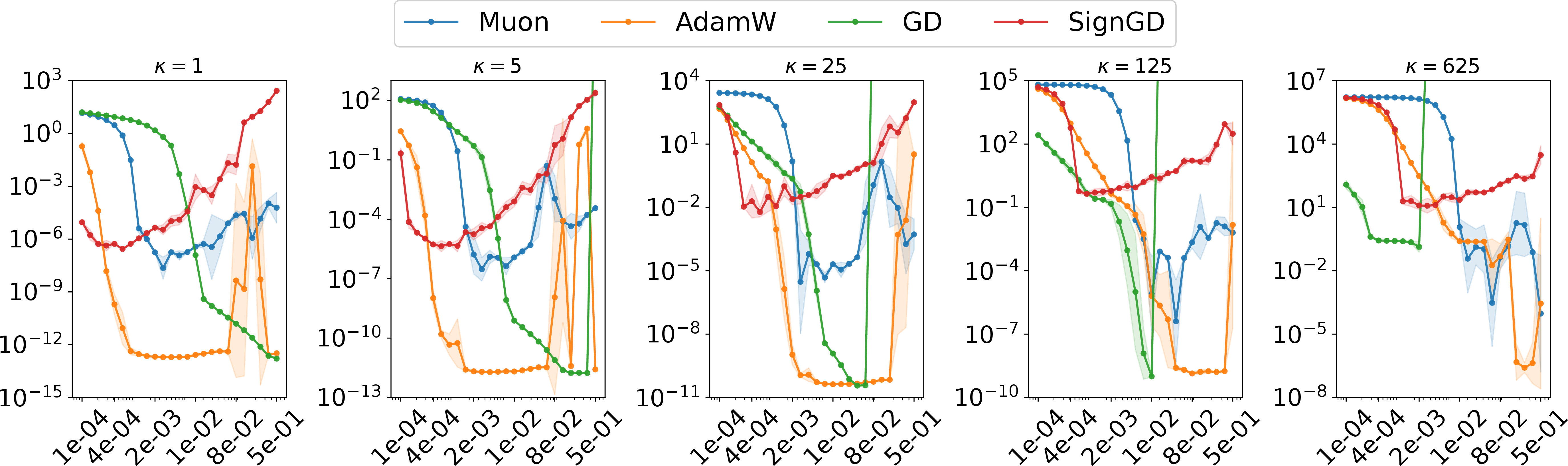
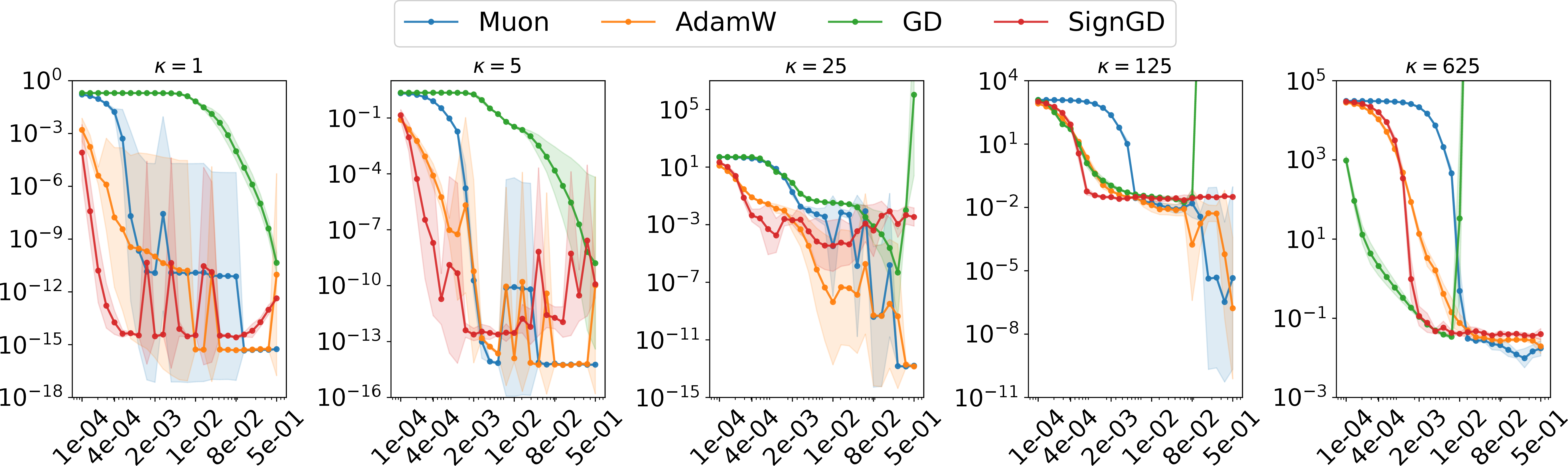
Low-rank factorization (conditioning). A fully observed target \(M^{\star}=U^{\star}\mathrm{diag}(\sigma)U^{\star\top}\) of rank \(r=15\) (i.e., we solve for the symmetric factorization) whose singular values are spaced linearly between \(\kappa\) and \(1\), so \(\kappa\in\{1,5,25,125,625\}\) is exactly the condition number. Objective \(\tfrac{1}{4}\lVert UU^{\top}-M^{\star}\rVert_{F}^{2}\) (Figure 1).
Matrix completion (conditioning). A rank-\(4\) symmetric PSD target with the same conditioning sweep, observed on a uniformly random \(20\%\) of entries; loss \(\tfrac{1}{2}\lVert\mathcal{P}_\Omega(UV^{\top}-M^{\star})\rVert_{F}^{2}\), the squared error on the observed support (Figure 7).
Matrix completion (over-parameterization). The same completion task at fixed \(\kappa=5\) and true rank \(4\), sweeping the search rank \(k\in\{4,5,100\}\) (matched, mildly, and heavily over-parameterized) (Figure 8).
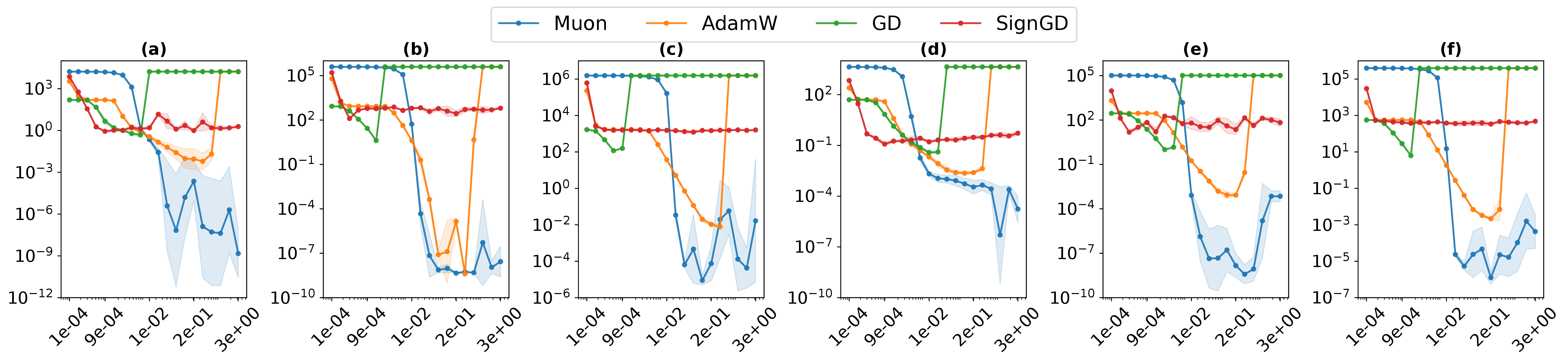
Non-negative factorization. A non-negative target with a projected (\(\,\cdot\,\geq 0\)) parameterization, at factor rank \(k\in\{10,50,100\}\), under two target spectra: a uniform spectrum and a decayed (exponentially graded) spectrum, the latter removing the flat “DC-component” degeneracy of the uniform case (Figure 2).
Tensor-train factorization (over-parameterization, noise). A symmetric positive semidefinite target \(M^{\star}=U^{\star}U^{\star\top}\) recovered with untied cores \(U,V\) in a noiseless (\(r^{\star}=4\)) and a noisy (\(r^{\star}=30\)) regime, sweeping the search rank across under-, exactly-, and over-parameterized values. Objective \(\tfrac{1}{2}\lVert UV^{\top}-M^{\star}\rVert_{F}^{2}\); see Section 4.3 and Figures 5 and 9.
We compare Muon (momentum \(0.95\), Nesterov, \(5\) Newton–Schulz orthogonalization steps) against AdamW, plain gradient descent (GD), and sign gradient descent (SignGD).
3.2 Evaluation protocol↩︎
We evaluate recovery with the normalized mean-squared error (NMSE), the squared reconstruction error relative to \(\left\lVert {\boldsymbol{M}}^\star \right\rVert_{\mathrm{F}}^2\), which makes the metric
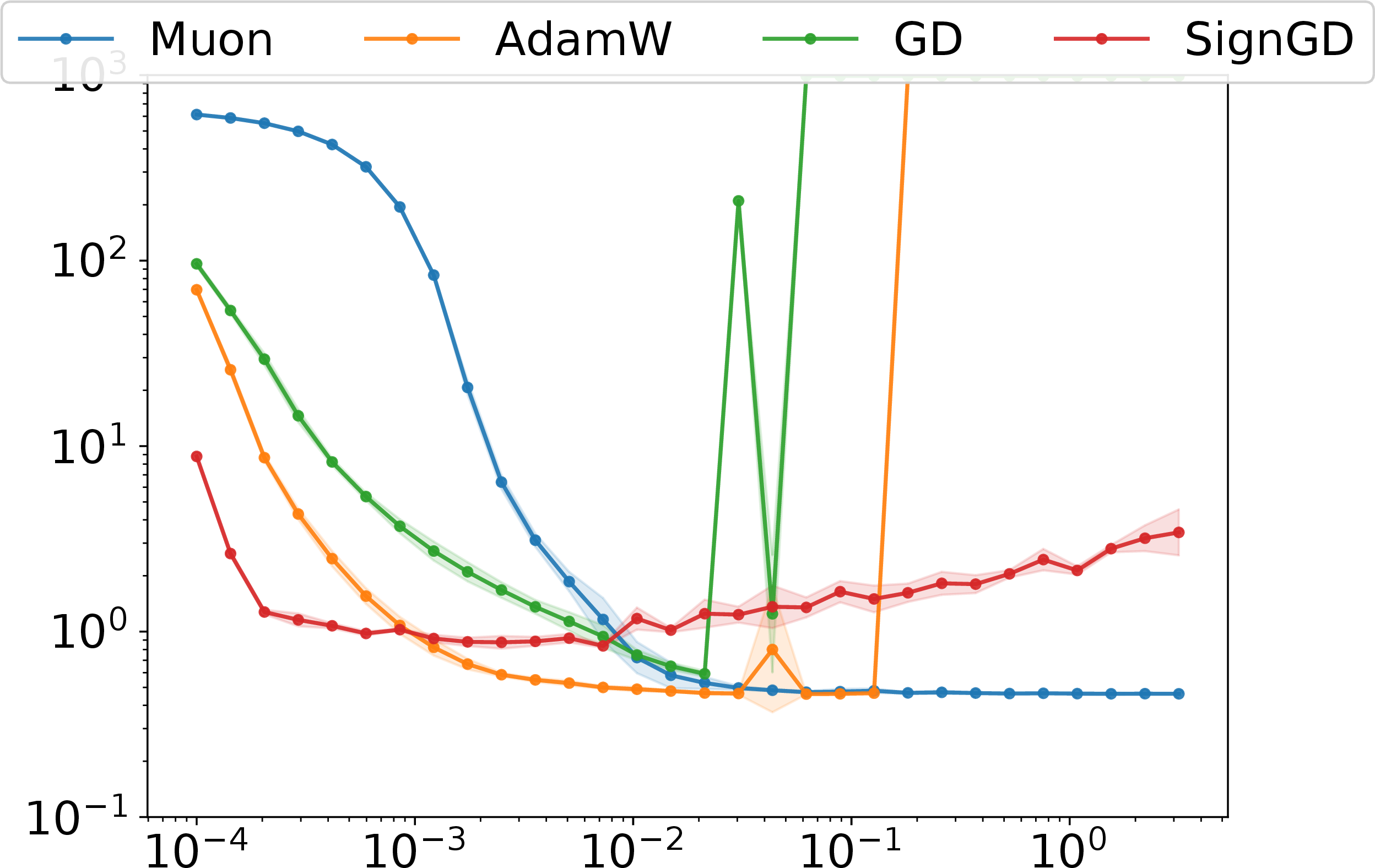
scale-free and comparable across problems and conditioning regimes. For every (problem, condition, optimizer) triple we sweep the learning rate, the dominant axis and the usual source of misleading comparisons, over a logarithmically spaced grid (\(25\) points in \([10^{-4},5\times10^{-1}]\) for the factorization and completion tasks; \(20\) points in \([10^{-4},3.2]\) for
NMF), holding all other hyperparameters (momentum, and for Muon the Newton–Schulz count \(J\) and the orthogonalization coefficients) at standard values. Each configuration runs for up to \(3000\) iterations under an identical patience-based learning-rate-decay schedule and is repeated over \(3\) seeds. Because the resulting NMSE values span roughly thirty orders of magnitude, we
summarize each configuration by the geometric mean over seeds with a \(\pm\)one-log-standard-deviation band, and compare optimizers by their stable learning-rate range, the band of step sizes over which
each converges to the NMSE floor.
4 Experimental Results↩︎
A single learning rate is not a meaningful operating point. Within a fixed problem and optimizer, the final loss varies by a median of about \(11\) orders of magnitude across the learning-rate grid for the factorization and completion tasks, and about \(6\) orders for both NMF variants (Figures 1–2). Performance is therefore dominated by the learning rate, and any comparison made at one pre-selected value reflects that choice as much as the optimizer itself.
No shared learning rate is fair to all methods. The loss-minimizing learning rate differs across optimizers by a median of \(1.5\)–\(3.1\) decades (largest for NMF), so evaluating all methods at a common learning rate necessarily places at least one of them far from its own optimum. This appears as a horizontal shift between each method’s basin in every panel.
Tuning reorders the methods, and the winner is problem-dependent. Table 1 reports each optimizer’s best (learning-rate-tuned) final loss. In nearly all nineteen settings the ranking induced by a fixed “default” learning rate (\(\approx 10^{-3}\)) differs from the ranking obtained once each method is tuned individually, and methods that look worst at the default frequently become best after tuning. Under per-optimizer tuning no method dominates universally: AdamW and GD win on plain low-rank factorization, Muon and AdamW are comparable on matrix completion, and Muon wins clearly on both NMF variants. The detailed per-setting comparisons, including the specific default-vs-tuned reorderings, are deferred to Appendix 9.
Ill-conditioning widens the gaps and shifts the winner. Conditioning is itself a hyperparameter of the problem, and it interacts strongly with the optimizer. As \(\kappa\) grows, every method’s attainable loss degrades and its optimal learning rate migrates upward (Figures 1, 7). The effect is most dramatic for the non-adaptive methods on factorization, where GD goes from the best-tuned method in the well-conditioned regime to failing under extreme ill-conditioning while AdamW becomes best (see Appendix 9 for the precise values). Thus ill-conditioning does not merely raise the loss floor, it reorders the methods, so that no fixed configuration summarizes behavior across the conditioning range.
4.1 Sensitivity to spectrum shape under extreme ill-conditioning↩︎
Conditioning alone does not determine difficulty: at a fixed condition number, the convergence of first-order optimizers also depends on the distribution of eigenvalues within \([s_{\min}, s_{\max}]\). We therefore hold the conditioning fixed at an extreme value and vary only the interior shape of the spectrum, evaluating seven spectral profiles (defined in Appendix 11). All seven families share the same endpoints \((s_{\min}, s_{\max}) = (10^{-3}, 10)\) and hence the same, deliberately extreme, condition number \(\kappa = s_{\max}/s_{\min} = 10^{4}\); only the interior shape differs. Despite this identical (and severe) ill-conditioning, the distributions pose markedly different preconditioning challenges. As shown in Figure 3, AdamW adapts effectively to heavy-tailed and clustered spectra, whereas Muon underperforms across the majority of these shapes, evidence that its spectral updates are less robust to specific eigenvalue densities even when the overall condition number is held fixed. Ill-conditioning is therefore not a single axis of difficulty: the same \(\kappa\) can be easy or hard depending on how the eigenvalues are arranged, and the two optimizers respond to that arrangement differently.
4.2 Gaussian-kernel factorization: a well-behaved landscape↩︎
To complement the synthetic NMF problems, we study the Gaussian radial-basis-function kernel. We sample \(N=100\) points in \(\mathbb{R}^{5}\) and form \(K_{ij}=\exp(-\lVert x_i-x_j\rVert^2/ 2\sigma^2)\) with \(\sigma=2\), giving a symmetric positive-semidefinite matrix with strictly positive entries and a rapidly decaying spectrum. We factorize it as \(\hat{K}=UV^{\top}\) under a non-negativity constraint (\(U,V\geq 0\), enforced by projection after each step), minimizing \(\tfrac{1}{2}\lVert UV^{\top}-K\rVert_F^2\).
Rather than fix the factor rank arbitrarily, we set it by a principled bottleneck: the smallest rank \(r\) whose leading singular values capture at least \(95\%\) of \(K\)’s spectral energy, which yields \(r=24\) for this target. Each optimizer is tuned by a learning-rate sweep (\(30\) points in \([10^{-4},10^{0.5}]\)), and every configuration is repeated over three seeds that vary the initialization while holding the target fixed.
The result is shown in Figure 10. On this well-behaved landscape, Muon’s advanced orthogonalization is unnecessary: standard AdamW performs just as effectively, converging seamlessly to the same global floor as Muon. This reinforces the study’s central theme from the opposite direction, on the adversarial NMF spectra Muon’s structured updates help, but on a smooth, well-conditioned kernel target that advantage disappears and a well-tuned adaptive baseline is equally good.
4.3 Tensor-train factorization↩︎
We consider the tensor-train (TT) factorization of a matrix target. For an order-\(2\) tensor \({\boldsymbol{M}}^\star \in \mathbb{R}^{d \times d}\), the TT decomposition contracts two cores \(\mathcal{G}_1 \in \mathbb{R}^{d \times r}\) and \(\mathcal{G}_2 \in \mathbb{R}^{r \times d}\) with boundary ranks \(r_0 = r_2 = 1\) and a single internal rank \(r_1 = r\), \[{\boldsymbol{M}}^\star(i,j) \;=\; \sum_{\alpha=1}^{r} \mathcal{G}_1(i,\alpha)\,\mathcal{G}_2(\alpha,j) , \qquad\Longleftrightarrow\qquad {\boldsymbol{M}}^\star \;=\; \mathcal{G}_1 \mathcal{G}_2 , \label{eq:tt-contraction}\tag{4}\] so the TT factorization coincides with the bilinear factorization of Appendix 7 under \({\boldsymbol{U}}= \mathcal{G}_1\), \({\boldsymbol{V}}^\top = \mathcal{G}_2\), with the lone TT-rank \(r\) playing the role of the factorization rank. In our setting the target \({\boldsymbol{M}}^\star = {\boldsymbol{U}}^\star {\boldsymbol{U}}^{\star\top}\) is symmetric positive semidefinite, but we do not tie the cores: recovery uses untied factors \({\boldsymbol{U}}, {\boldsymbol{V}}\), so the problem is the general bilinear factorization equation 12 applied to a symmetric PSD target, retaining the \(\mathrm{GL}_r\) imbalance invariance of equation 12 . Recovery minimizes \[f({\boldsymbol{U}}, {\boldsymbol{V}}) \;=\; \frac{1}{2}\,\left\lVert {\boldsymbol{U}}{\boldsymbol{V}}^\top - {\boldsymbol{M}}^\star \right\rVert_{\mathrm{F}}^2 , \qquad {\boldsymbol{U}}\in \mathbb{R}^{d \times r}, {\boldsymbol{V}}\in \mathbb{R}^{d \times r}, \label{eq:tt-objective}\tag{5}\] the objective of equation 12 with search rank \(r\) as the TT-rank.
We study equation 5 in two regimes, a noiseless regime (true rank \(r^\star = 4\), recovered exactly, loss limited only by convergence) and a noisy regime (true rank \(r^\star = 30\) with additive observation noise, loss floored at the statistical noise level), and within each we sweep the search rank across under-, exactly-, and over-parameterized values; full specifications are given in Appendix 12. The quantity of interest is the stable learning-rate range of each optimizer, the band of step sizes over which equation 5 converges to its regime-dependent floor, and how that band widens, narrows, or shifts as the parameterization regime and the noise level change (Figures 5 and 9). Beyond low-rank recovery, this factorized objective serves as a minimal model of the product parameterizations ubiquitous in deep learning, a connection we develop in Appendix 13. We also study the effect of factorization depth in Appendix 14.
5 Conclusion↩︎
In this work, we revisit optimizer comparisons for matrix factorization and show that conclusions are highly sensitive to hyperparameter selection and problem conditioning. Systematic learning-rate sweeps reveal that rankings reported under single configurations often do not hold: well-tuned AdamW and gradient descent frequently match or outperform Muon on standard low-rank factorization tasks, while Muon’s advantages are mostly limited to NMF and some highly ill-conditioned completion problems. We further find that optimizer performance depends on both conditioning severity and spectral structure, altering method rankings across problem instances. These results underscore the need to evaluate optimizers across tuned hyperparameter ranges and conditioning regimes rather than relying on default settings or isolated benchmarks.
Acknowledgements↩︎
We thank Tianhao Wang for providing helpful references and for the discussions that assisted in developing the experimental setup. Ali Parviz was funded by NSF CIF-2403452.
| Problem | Setting | Muon | AdamW | GD | SignGD |
|---|---|---|---|---|---|
| Factorization | \(\kappa{=}1\) | \(2.3\!\times\!10^{-8}\) | \(1.9\!\times\!10^{-13}\) | \(\mathbf{1.6\!\times\!10^{-13}}\) | \(2.8\!\times\!10^{-7}\) |
| \(\kappa{=}5\) | \(3.0\!\times\!10^{-7}\) | \(1.9\!\times\!10^{-12}\) | \(\mathbf{1.7\!\times\!10^{-12}}\) | \(4.4\!\times\!10^{-6}\) | |
| \(\kappa{=}25\) | \(3.0\!\times\!10^{-6}\) | \(4.2\!\times\!10^{-11}\) | \(\mathbf{3.7\!\times\!10^{-11}}\) | \(6.1\!\times\!10^{-3}\) | |
| \(\kappa{=}125\) | \(4.1\!\times\!10^{-7}\) | \(1.4\!\times\!10^{-9}\) | \(\mathbf{1.0\!\times\!10^{-9}}\) | \(4.4\!\times\!10^{-1}\) | |
| \(\kappa{=}625\) | \(9.4\!\times\!10^{-5}\) | \(\mathbf{2.6\!\times\!10^{-7}}\) | \(1.3\!\times\!10^{-1}\) | \(1.2\!\times\!10^{1}\) | |
| Completion (\(\kappa\)) | \(\kappa{=}1\) | \(\mathbf{4.6\!\times\!10^{-16}}\) | \(4.8\!\times\!10^{-16}\) | \(4.5\!\times\!10^{-11}\) | \(2.6\!\times\!10^{-15}\) |
| \(\kappa{=}5\) | \(5.7\!\times\!10^{-15}\) | \(\mathbf{5.5\!\times\!10^{-15}}\) | \(1.6\!\times\!10^{-9}\) | \(2.4\!\times\!10^{-13}\) | |
| \(\kappa{=}25\) | \(\mathbf{1.4\!\times\!10^{-13}}\) | \(1.4\!\times\!10^{-13}\) | \(4.7\!\times\!10^{-7}\) | \(3.5\!\times\!10^{-5}\) | |
| \(\kappa{=}125\) | \(3.3\!\times\!10^{-7}\) | \(\mathbf{1.7\!\times\!10^{-7}}\) | \(1.8\!\times\!10^{-2}\) | \(2.2\!\times\!10^{-2}\) | |
| \(\kappa{=}625\) | \(\mathbf{9.8\!\times\!10^{-3}}\) | \(2.0\!\times\!10^{-2}\) | \(3.4\!\times\!10^{-2}\) | \(3.6\!\times\!10^{-2}\) | |
| Completion (rank) | \(r{=}4\) | \(5.7\!\times\!10^{-15}\) | \(\mathbf{5.5\!\times\!10^{-15}}\) | \(1.6\!\times\!10^{-9}\) | \(2.4\!\times\!10^{-13}\) |
| \(r{=}5\) | \(\mathbf{4.5\!\times\!10^{-15}}\) | \(1.8\!\times\!10^{-12}\) | \(2.1\!\times\!10^{-6}\) | \(4.9\!\times\!10^{-8}\) | |
| \(r{=}100\) | \(2.1\!\times\!10^{-15}\) | \(\mathbf{1.5\!\times\!10^{-15}}\) | \(1.8\!\times\!10^{-14}\) | \(3.2\!\times\!10^{-15}\) | |
| NMF (uniform) | \(r{=}10\) | \(\mathbf{1.5\!\times\!10^{-9}}\) | \(6.1\!\times\!10^{-3}\) | \(4.8\!\times\!10^{-1}\) | \(8.7\!\times\!10^{-1}\) |
| \(r{=}50\) | \(4.5\!\times\!10^{-9}\) | \(\mathbf{4.1\!\times\!10^{-9}}\) | \(4.1\!\times\!10^{0}\) | \(1.3\!\times\!10^{2}\) | |
| \(r{=}100\) | \(\mathbf{8.9\!\times\!10^{-6}}\) | \(7.8\!\times\!10^{-3}\) | \(1.2\!\times\!10^{2}\) | \(1.2\!\times\!10^{3}\) | |
| NMF (decay) | \(r{=}10\) | \(\mathbf{5.1\!\times\!10^{-7}}\) | \(2.3\!\times\!10^{-3}\) | \(3.8\!\times\!10^{-2}\) | \(1.2\!\times\!10^{-1}\) |
| \(r{=}50\) | \(\mathbf{3.8\!\times\!10^{-9}}\) | \(8.4\!\times\!10^{-4}\) | \(1.0\!\times\!10^{0}\) | \(1.5\!\times\!10^{1}\) | |
| \(r{=}100\) | \(\mathbf{1.2\!\times\!10^{-6}}\) | \(2.1\!\times\!10^{-3}\) | \(6.3\!\times\!10^{0}\) | \(3.4\!\times\!10^{2}\) |
6 Background: The Muon Optimizer↩︎
We briefly recall the Muon update and the spectral viewpoint that motivates it. Consider a weight matrix \({\boldsymbol{W}}\in \mathbb{R}^{m \times n}\) with loss gradient \({\boldsymbol{G}}_t = \nabla_{{\boldsymbol{W}}}L({\boldsymbol{W}}_t)\) at iteration \(t\). Muon maintains a momentum buffer \({\boldsymbol{B}}_t\)
and applies an orthogonalized update: \[\begin{align} {\boldsymbol{B}}_t &= \mu\, {\boldsymbol{B}}_{t-1} + {\boldsymbol{G}}_t, \tag{6}\\ {\boldsymbol{O}}_t &=
\operatorname{Newton\text{-}Schulz}({\boldsymbol{B}}_t) \;\approx\; \operatorname{polar}({\boldsymbol{B}}_t), \tag{7}\\ {\boldsymbol{W}}_{t+1} &= {\boldsymbol{W}}_t - \alpha\, {\boldsymbol{O}}_t. \tag{8}
\end{align}\] Here \(\alpha> 0\) is the step
size and \(\mu\in [0,1)\) the momentum coefficient. The orthogonalization step equation 7 replaces the momentum direction by (an approximation of) its polar factor.
Polar factor and spectral steepest descent. Let \({\boldsymbol{B}}_t = {\boldsymbol{P}}{\boldsymbol{\Sigma}}{\boldsymbol{Q}}^\top\) be a singular value decomposition, with \({\boldsymbol{P}}\in \mathcal{O}_{m \times \rho}\), \({\boldsymbol{Q}}\in \mathcal{O}_{n \times \rho}\), and \({\boldsymbol{\Sigma}}= \mathsf{diag}\{\sigma_1, \dots,
\sigma_\rho\}\), where \(\rho = \mathrm{rank}({\boldsymbol{B}}_t)\). The polar factor is \[\operatorname{polar}({\boldsymbol{B}}_t) \;=\;
{\boldsymbol{P}}{\boldsymbol{Q}}^\top, \label{eq:polar}\tag{9}\] which sets every nonzero singular value to one while preserving the singular vectors. Equivalently, \({\boldsymbol{P}}{\boldsymbol{Q}}^\top\) is
the solution of the spectral-norm linear minimization oracle, \[{\boldsymbol{P}}{\boldsymbol{Q}}^\top \;=\; \mathop{\mathrm{arg\,max}}_{\left\lVert {\boldsymbol{X}} \right\rVert_{\mathrm{op}}
\le 1} \left\langle {\boldsymbol{B}}_t, {\boldsymbol{X}} \right\rangle, \label{eq:lmo}\tag{10}\] so the Muon direction equation 7 is precisely the steepest-descent direction with respect to the
spectral norm. This is the sense in which Muon is “spectrum aware”: it discards the magnitude of the momentum’s singular values and acts only along their directions.
Newton–Schulz orthogonalization. Computing the SVD at every step is expensive, so Muon approximates the polar factor with a fixed number of matrix-multiplication-only Newton–Schulz iterations. Starting from the normalized
matrix \({\boldsymbol{X}}_0 = {\boldsymbol{B}}_t / \left\lVert {\boldsymbol{B}}_t \right\rVert_{\mathrm{F}}\), one iterates a fixed odd polynomial \[{\boldsymbol{X}}_{j+1} \;=\; a\,{\boldsymbol{X}}_j \;+\; b\,{\boldsymbol{X}}_j {\boldsymbol{X}}_j^\top {\boldsymbol{X}}_j \;+\; c\,\big({\boldsymbol{X}}_j {\boldsymbol{X}}_j^\top\big)^2 {\boldsymbol{X}}_j, \qquad j = 0, 1, \dots,
J-1, \label{eq:newton-schulz}\tag{11}\] with coefficients \((a,b,c)\) chosen so that the induced scalar map \(\sigma \mapsto a\sigma + b\sigma^3 + c\sigma^5\) pushes the
singular values of \({\boldsymbol{X}}_j\) toward \(1\). The quintic coefficients \((a,b,c) = (3.4445, -4.7750, 2.0315)\) proposed by [1] reach a usable approximation in roughly \(J = 5\) iterations; subsequent work designs improved polynomials for this
orthogonalization [19]–[22]. As \(J \to \infty\) (with an exact map) the iteration converges to \(\operatorname{polar}({\boldsymbol{B}}_t)\), recovering the idealized update; in
practice \(J\) is small and \({\boldsymbol{O}}_t\) is only an approximate polar factor, which several recent analyses account for explicitly [13]–[15].
7 Matrix Factorization Variants↩︎
This appendix collects two generalizations of the symmetric matrix factorization problem equation 1 : the general bilinear (asymmetric) factorization and the matrix completion setting in which only a subset of the entries of the target is observed.
7.0.0.1 General bilinear factorization.
The symmetric problem equation 1 is a special case of the general bilinear (asymmetric) factorization, in which a possibly rectangular target \({\boldsymbol{M}}^\star \in \mathbb{R}^{d_1 \times d_2}\) of rank \(r\) is recovered from the product of two factors, \[\min_{\substack{{\boldsymbol{U}}\in \mathbb{R}^{d_1 \times k}\\[2pt] {\boldsymbol{V}}\in \mathbb{R}^{d_2 \times k}}}\quad f({\boldsymbol{U}}, {\boldsymbol{V}}) \;=\; \frac{1}{2}\,\left\lVert {\boldsymbol{U}}{\boldsymbol{V}}^\top - {\boldsymbol{M}}^\star \right\rVert_{\mathrm{F}}^2 , \label{eq:bmf}\tag{12}\] with \(k \ge r\). When \({\boldsymbol{M}}^\star\) is symmetric positive semidefinite and the factors are tied as \({\boldsymbol{V}}= {\boldsymbol{U}}\), equation 12 reduces to equation 1 up to a constant rescaling of the objective. Unlike the symmetric case, the asymmetric parameterization is invariant under the larger group of invertible transformations \(({\boldsymbol{U}}, {\boldsymbol{V}}) \mapsto ({\boldsymbol{U}}{\boldsymbol{R}}, {\boldsymbol{V}}{\boldsymbol{R}}^{-\top})\) for any \({\boldsymbol{R}}\in \mathrm{GL}_k(\mathbb{R})\), since \({\boldsymbol{U}}{\boldsymbol{V}}^\top = ({\boldsymbol{U}}{\boldsymbol{R}})({\boldsymbol{V}}{\boldsymbol{R}}^{-\top})^\top\). This invariance permits an arbitrary imbalance between the factor norms and is commonly controlled by a balancing regularizer \(\tfrac{1}{2}\bigl(\left\lVert {\boldsymbol{U}} \right\rVert_{\mathrm{F}}^2 + \left\lVert {\boldsymbol{V}} \right\rVert_{\mathrm{F}}^2\bigr)\) or by enforcing \({\boldsymbol{U}}^\top {\boldsymbol{U}}= {\boldsymbol{V}}^\top {\boldsymbol{V}}\) along the trajectory.
7.0.0.2 Matrix completion.
In many applications only a subset of the entries of \({\boldsymbol{M}}^\star\) is observed. Let \([n] \mathrel{\vcenter{:}}= \{1, \dots, n\}\) and let \(\Omega \subseteq [d_1] \times [d_2]\) denote the set of observed indices. Define the sampling operator \(\mathcal{P}_\Omega : \mathbb{R}^{d_1 \times d_2} \to \mathbb{R}^{d_1 \times d_2}\) by \[\bigl[\mathcal{P}_\Omega({\boldsymbol{X}})\bigr]_{ij} \;=\; \begin{cases} X_{ij}, & (i,j) \in \Omega,\\[2pt] 0, & \text{otherwise,} \end{cases} \label{eq:sampling-operator}\tag{13}\] which retains the observed entries and zeros out the rest. The factored matrix completion problem is \[\min_{\substack{{\boldsymbol{U}}\in \mathbb{R}^{d_1 \times k}\\[2pt] {\boldsymbol{V}}\in \mathbb{R}^{d_2 \times k}}}\quad \frac{1}{2}\,\left\lVert \mathcal{P}_\Omega\!\bigl({\boldsymbol{U}}{\boldsymbol{V}}^\top - {\boldsymbol{M}}^\star\bigr) \right\rVert_{\mathrm{F}}^2 . \label{eq:mc}\tag{14}\] Taking \(\Omega = [d_1] \times [d_2]\) recovers the fully observed problem equation 12 , while the symmetric variant tied to equation 1 additionally imposes \({\boldsymbol{V}}= {\boldsymbol{U}}\). Exact recovery in this setting requires the ground-truth factors to be incoherent and the sample size \(\lvert \Omega \rvert\) to be sufficiently large relative to the degrees of freedom \(r(d_1 + d_2 - r)\). Under the Bernoulli model in which each entry is observed independently with probability \(p\), the rescaled operator \(p^{-1}\mathcal{P}_\Omega\) is an unbiased estimator of the identity, i.e.\(\mathbb{E}\bigl[p^{-1}\mathcal{P}_\Omega({\boldsymbol{X}})\bigr] = {\boldsymbol{X}}\).
8 Related Work↩︎
Spectrum-aware optimization and Muon. Much of the theoretical analysis of Muon builds on a perspective that interprets modern optimizers such as Adam and Shampoo as instances of
steepest descent under non-Euclidean or norm-constrained geometries [23]. Within this view, Muon approximates a spectral-norm
steepest-descent direction via polar factorization, connecting it to a broader class of methods that leverage matrix structure in gradients [4]–[7]. Spectral transformations and orthogonalization in optimization predate Muon, appearing in earlier work on stochastic and preconditioned methods [24]–[27]. A complementary line of work asks more directly when such spectral updates are beneficial in deep learning [16], [17].


Implicit bias and generalization. A second line of work studies the implicit bias induced by Muon. [28] show
that in linear classification, idealized Muon converges to a solution that maximizes margin with respect to the spectral norm, contrasting with the Euclidean and coordinate-wise biases of SGD and Adam. Complementary
empirical studies suggest that spectrum-aware updates can improve generalization, particularly in imbalanced or long-tailed settings, by promoting more uniform learning across principal components rather than focusing on dominant directions [29], [30]. Related analyses indicate that Muon yields more
isotropic singular-value spectra than Adam and may accelerate phenomena such as grokking in long-horizon training [29]–[32]. Connections have also been drawn between Muon and second-order or preconditioned methods, with several works
interpreting its updates as approximations to Shampoo[1], [33], [34]. Alternative derivations and closely related formulations, some predating Muon, have appeared from different theoretical viewpoints [15], [23], [26], [35]–[37].
Preconditioning for matrix factorization. A separate body of work shows that preconditioning can dramatically accelerate optimization in matrix factorization. In particular, ScaledGD and its variants achieve linear
convergence rates independent of the condition number under appropriate initialization, in both exactly parameterized and over-parameterized regimes [38]–[41], and these
guarantees extend to small random initialization [42]. Closest to our motivation, recent work analyzes the preconditioning effect of
Muon’s spectral orthogonalization directly [18].
Summary. Taken together, these results show that spectrum-aware and preconditioned methods can offer strong theoretical and empirical benefits, but that their behavior depends heavily on problem structure and initialization. This
motivates a closer examination of Muon in controlled settings such as matrix factorization, where powerful alternatives already enjoy strong guarantees and where the advantage of Muon over adaptive methods like AdamW
is not immediately evident.
9 Detailed experimental results↩︎
This appendix expands the summary claims of Section 4 with the specific numerical comparisons. All values refer to Table 1.
9.0.0.1 Horizontal basin shifts.
Evaluating all methods at a common learning rate necessarily places at least one of them far from its own optimum. This is visible as a horizontal shift between each method’s basin in every panel: for instance, GD’s basin lies near the high end of the grid while Muon’s and AdamW’s lie one to three decades lower.
9.0.0.2 Default-vs-tuned reordering.
The ranking induced by a fixed default learning rate (\(\approx 10^{-3}\)) differs from the tuned ranking in nearly all nineteen settings, and methods that look worst at the default frequently become best after tuning. On low-rank factorization GD is among the worst at the default rate yet attains the lowest loss of all methods once tuned (Figure 1); symmetrically, on both NMF variants Muon is last at the default rate but first once tuned (Figures 2).
9.0.0.3 Effect of ill-conditioning.
The effect of ill-conditioning is most dramatic for the non-adaptive methods on factorization: GD, the best-tuned method in the well-conditioned regime (\(1.6\times10^{-13}\) at \(\kappa{=}1\)), collapses to \(1.3\times10^{-1}\) at \(\kappa{=}625\), where AdamW becomes best (\(2.6\times10^{-7}\)), Muon second (\(9.4\times10^{-5}\)), and SignGD diverges. Matrix completion shows the same upward drift of the loss floor: at \(\kappa{=}625\) all four methods are confined to \(O(10^{-2})\) and become nearly indistinguishable.
9.0.0.4 Problem-dependence of the tuned winner.
Under per-optimizer tuning there is no universally dominant method. On plain low-rank factorization, AdamW and GD drive the loss to \(10^{-13}\)–\(10^{-9}\) across the whole conditioning range, while the Muon configuration plateaus several orders higher (\(10^{-8}\)–\(10^{-5}\)). On matrix completion, Muon and AdamW are both reaching \(10^{-16}\)–\(10^{-13}\) in the well-conditioned regime, and over-parameterization (search rank \(100\)) lets all methods except GD reach machine precision (Figure 8). On NMF, the picture reverses: Muon is the clear winner under both spectra, reaching \(10^{-9}\)–\(10^{-6}\) while AdamW stalls near \(10^{-3}\) (with the single exception of the uniform-spectrum rank-\(50\) case, where AdamW matches Muon at \(\sim 4\times10^{-9}\)) and GD/SignGD fail to fit. Whichever optimizer a single-configuration study would crown thus depends entirely on the problem and the learning rate chosen.
10 Dynamics of spectral subspace recovery↩︎
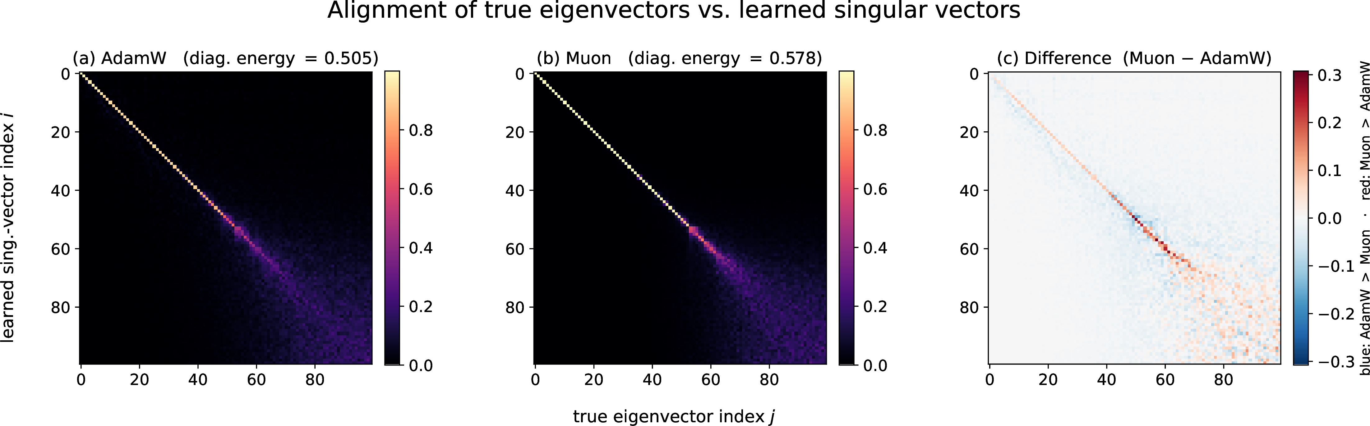
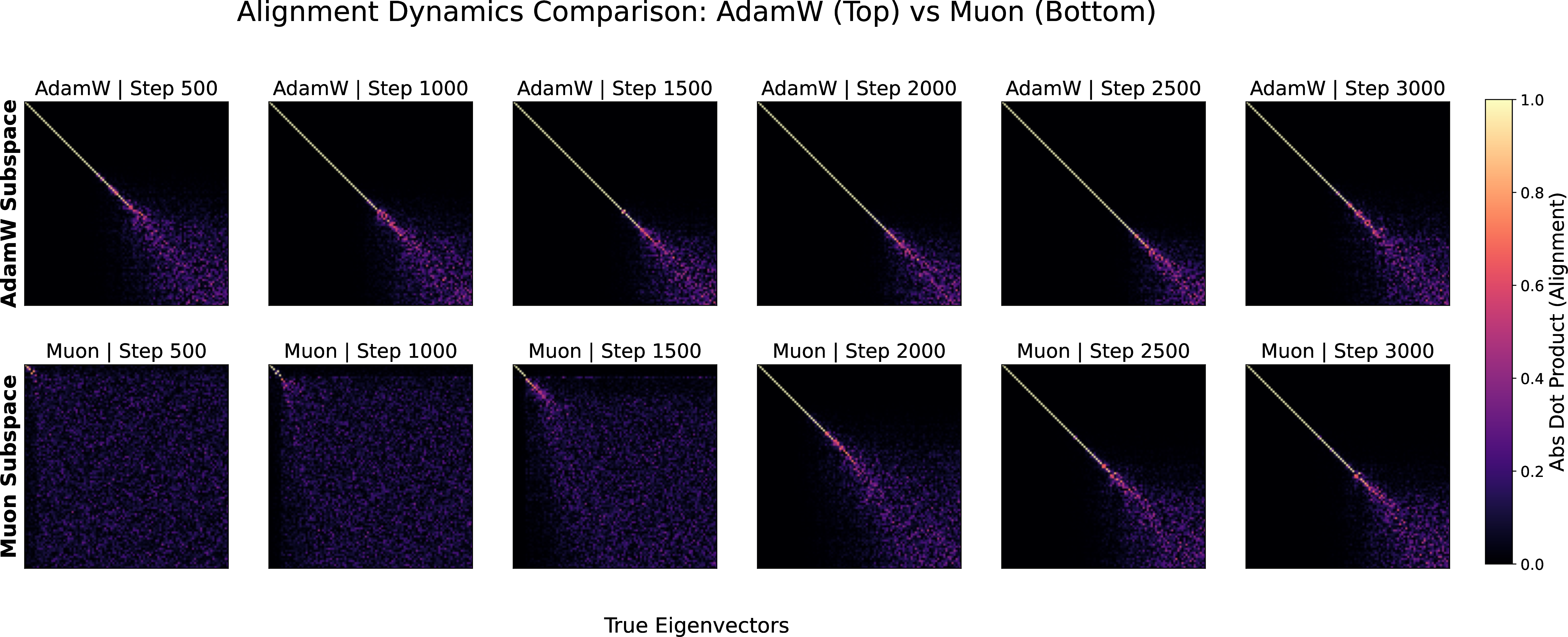
The aggregate losses above tell us whether a method fits the target but not how it does so. To probe the mechanism, we factorize a fixed Gaussian-kernel target \(K \in \mathbb{R}^{100 \times 100}\), symmetric positive semidefinite, with eigendecomposition \(K = Q\Lambda Q^{\top}\) and eigenvectors ordered by descending eigenvalue, as \(\hat{K} = UV^{\top}\) at full search rank \(k = 100\), training AdamW and Muon each at its own tuned learning rate. Every \(500\) iterations we take the left singular vectors \(\{\hat{u}_i\}\) of the current reconstruction \(UV^{\top}\) and form the alignment matrix \[M_{ij} \;=\; \bigl|\langle \hat{u}_i,\; q_j \rangle\bigr|, \label{eq:alignment}\tag{15}\] the absolute overlap between the \(i\)-th learned singular direction and the \(j\)-th true eigenvector. A faithful, correctly ordered recovery of the eigenbasis yields \(M \to I\) (a sharp diagonal), whereas off-diagonal or diffuse mass indicates that the learned subspace mixes or reorders eigendirections. Figure 6 tracks \(M\) over training. AdamW sharpens toward a clean diagonal quickly and monotonically, recovering the eigenvectors faithfully and in order, while Muon’s alignment remains comparatively diffuse, with persistent off-diagonal mass and slower diagonalization. This provides a mechanistic explanation for the loss-level gap of Sections 4–4.1: on these structured and ill-conditioned spectra, AdamW’s per-coordinate adaptation locks onto the dominant eigendirections in the right order, whereas Muon’s orthogonalized updates distribute capacity more evenly across directions and recover the eigenbasis less cleanly. The heatmaps shown are for a representative tuned run; the qualitative pattern is consistent across seeds.
11 Spectral profile definitions↩︎
The experiments of Section 4.1 use seven spectral profiles, defined by the diagonal entries of \(S\). All share the endpoints \((s_{\min}, s_{\max}) = (10^{-3}, 10)\) and hence the condition number \(\kappa = s_{\max}/s_{\min} = 10^{4}\); only the interior shape differs.
Uniform: linear spacing \(s_i = s_{\min} + \frac{i-1}{n-1}(s_{\max}-s_{\min})\), a dense, even spread of curvature.
Log-uniform: geometric spacing \(s_i = s_{\min}\cdot\kappa^{\frac{i-1}{n-1}}\), typical of ill-conditioned systems whose scales vary by orders of magnitude.
Gaussian: eigenvalues drawn from a truncated normal \(\mathcal{N}(\mu,\sigma^2)\) and rescaled to \([s_{\min}, s_{\max}]\), a bulk concentrated around a mean curvature.
Spiked: a single top eigenvalue at \(s_{\max}\) with the remaining \(n-1\) clustered near \(s_{\min}\), a dominant rank-one subspace.
Bimodal: eigenvalues split into two clusters near the endpoints \(s_{\min}\) and \(s_{\max}\).
Polynomial decay: \(s_i \propto i^{-\alpha}\), a rapid decay in the importance of higher-order directions.
Exponential decay: \(s_i \propto e^{-\beta i}\), an aggressive concentration of energy in the top eigenvalues.
12 Tensor-train regimes and parameterization sweep↩︎
This appendix gives the full specification of the regimes and parameterization sweep summarized in Section 4.3.
12.0.0.1 Regimes.
We study equation 5 in two regimes. In the noiseless regime the target has true rank \(r^\star = 4\) and is recovered exactly, so the attainable loss is limited only by the optimizer’s convergence; in the noisy regime the target has true rank \(r^\star = 30\) and is corrupted by additive observation noise, so the loss is floored at the statistical noise level rather than driven to zero. The two regimes therefore probe complementary phenomena: optimization geometry in the well-specified case and robustness to a nonzero residual in the misspecified case.
12.0.0.2 Parameterization sweep.
Within each regime we sweep the search rank, equivalently the TT-rank \(r\) of the factor \({\boldsymbol{U}}\), across under-, exactly-, and over-parameterized values: \(r \in \{2, 4, 8, 20\}\) for the noiseless target (true rank \(r^\star = 4\)) and \(r \in \{5, 15, 30, 60\}\) for the noisy target (true rank \(r^\star = 30\)), with \(r = r^\star\) the exactly parameterized boundary case. Under-parameterization (\(r < r^\star\)) caps the attainable loss because \({\boldsymbol{U}}{\boldsymbol{U}}^\top\) cannot represent \({\boldsymbol{M}}^\star\), while over-parameterization (\(r > r^\star\)) enlarges the factor space and introduces additional flat directions in the landscape.
13 Relation to deep learning models↩︎
The factorized objective equation 5 is not only a tensor-train problem in its own right; it is the minimal instance of the product parameterizations that pervade deep learning, which is what makes the optimizer behavior we study here relevant beyond low-rank recovery.
13.0.0.1 Factorization as a shallow linear network.
The map \({\boldsymbol{U}}\mapsto {\boldsymbol{U}}{\boldsymbol{U}}^\top\) (or \(({\boldsymbol{U}},{\boldsymbol{V}})\mapsto{\boldsymbol{U}}{\boldsymbol{V}}^\top\) in the asymmetric case of Appendix 7) is exactly a two-layer linear network with no intervening nonlinearity: the factors are the layer weights, and the product is the end-to-end map. Consequently the loss is nonconvex in the factors despite being convex in the product, and the search rank, equivalently the TT-rank, plays the role of the network width. The over-parameterized regime \(r > r^\star\) is precisely the width-overparameterized regime of modern networks, and the flat directions it introduces in the landscape are the source of the implicit bias of gradient methods studied for matrix and deep factorizations [43], [44]. This is why over-parameterized factorization is a standard proxy for the optimization of deep models: it isolates the effect of redundant parameters on the trajectory while remaining analytically tractable.
13.0.0.2 Depth as a longer tensor-train chain.
Increasing the order of the tensor-train chain, contracting \(L\) cores \(\mathcal{G}_1,\dots,\mathcal{G}_L\) rather than two, is the algebraic analogue of increasing the depth of a linear network, whose end-to-end map factorizes as \({\boldsymbol{W}}= {\boldsymbol{W}}_L {\boldsymbol{W}}_{L-1}\cdots{\boldsymbol{W}}_1\). The matrix case equation 4 (\(L=2\)) is the shallowest such chain, and depth introduces exactly the ill-conditioning and balancing phenomena that motivate our conditioning sweep: the product of many factors amplifies spectral imbalance, and the overparameterized invariance group acts on each internal bond. Depth has been shown to act as an implicit preconditioner that accelerates gradient descent on these product objectives [45], so the sensitivity of each optimizer to conditioning at \(L=2\) is the base case of a phenomenon that sharpens with depth.
13.0.0.3 Tensor-train structure inside trained networks.
Beyond serving as a proxy, tensor-train factorizations appear directly inside deep models. Reshaping a dense weight matrix into a high-order tensor and representing it in TT format compresses fully connected and embedding layers by orders of magnitude while preserving accuracy [46], and specific architectures correspond to specific tensor decompositions: recurrent networks realize the tensor-train / matrix-product structure [47], while convolutional arithmetic circuits realize the hierarchical Tucker decomposition [48]. In all of these the rank of the decomposition controls expressivity exactly as the TT-rank \(r\) controls the capacity of equation 5 , so the interaction between search rank, conditioning, and optimizer that we characterize on the factorized problem speaks directly to how these layers are trained.
14 Optimizer Comparison Across Tensor-Train Depth↩︎
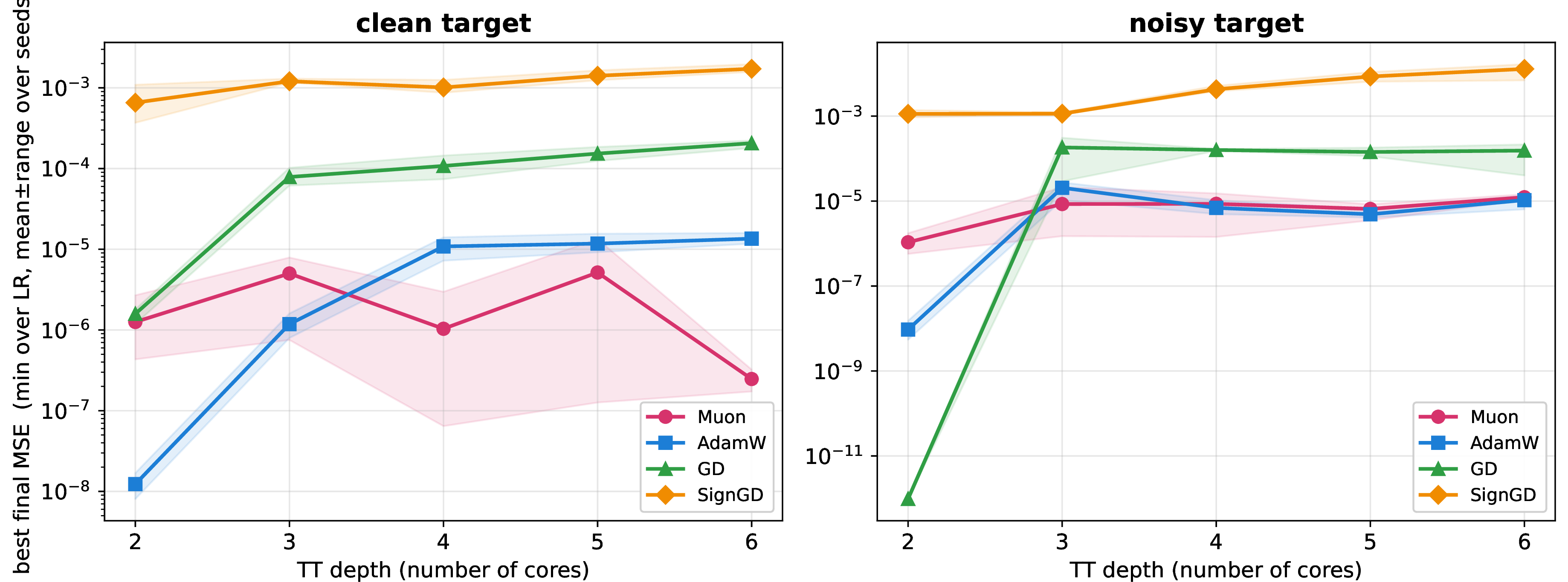
We benchmark four optimizers—Muon, AdamW, gradient descent (GD), and SignGD—on non-negative tensor-train (TT) factorization. To systematically vary problem conditioning, we use the tensor-train depth (equivalently, the tensor order or number of TT cores) as the primary experimental factor. Each TT core is represented via a matrix unfolding, a necessary implementation detail because Muon’s Newton–Schulz orthogonalization operates only on matrix-valued gradients; retaining a core in its native third-order form would effectively reduce Muon to momentum SGD on that factor. We evaluate two target regimes: a clean, low-rank, noise-free tensor and a noisy, higher-rank tensor. The study spans depths (2)–(6), an overparameterized factorization rank, a five-point learning-rate sweep, and three random seeds, yielding 600 total runs. Performance is reported as the best-tuned final loss for each optimizer, defined as the lowest mean squared error (MSE) achieved across the learning-rate grid and averaged over seeds.
The results differ markedly between the two regimes. For the clean target, optimizer rankings change substantially with depth. AdamW achieves the lowest losses at shallow depths, while Muon performs comparatively poorly. However, beginning at depth (4), the performance of AdamW, GD, and SignGD deteriorates as the factorization deepens, whereas Muon maintains consistently low error. By depth (6), Muon outperforms the competing methods by approximately one to two orders of magnitude (Figure 11, left). In contrast, performance on the noisy target remains relatively flat across depths, with all optimizers achieving similar losses (Figure 11, right). The added noise introduces an irreducible error floor that limits the optimization gains obtainable from improved conditioning, thereby diminishing Muon’s advantage.
These findings suggest that Muon’s benefits arise primarily from its ability to mitigate optimization difficulties associated with ill-conditioned deep factorizations, rather than from a general robustness advantage. At the same time, two limitations should be noted. First, increasing tensor-train depth changes the underlying optimization problem itself, so the observed trends reflect changes in relative optimizer performance across a family of increasingly difficult tasks rather than within a fixed loss landscape. Second, the reported results correspond only to the overparameterized setting considered here and may not fully characterize behavior at other scales or rank regimes.
15 Dynamics of spectral subspace recovery↩︎
The aggregate losses above tell us whether a method fits the target but not how it does so. To probe the mechanism, we factorize a fixed Gaussian-kernel target \(K \in \mathbb{R}^{100 \times 100}\), symmetric positive semidefinite, with eigendecomposition \(K = Q\Lambda Q^{\top}\) and eigenvectors ordered by descending eigenvalue, as \(\hat{K} = UV^{\top}\) at full search rank \(k = 100\), training AdamW and Muon each at its own tuned learning rate. Every \(500\) iterations we take the left singular vectors \(\{\hat{u}_i\}\) of the current reconstruction \(UV^{\top}\) and form the alignment matrix \[M_{ij} \;=\; \bigl|\langle \hat{u}_i,\; q_j \rangle\bigr|, \label{bpvwajid}\tag{16}\] the absolute overlap between the \(i\)-th learned singular direction and the \(j\)-th true eigenvector. A faithful, correctly ordered recovery of the eigenbasis yields \(M \to I\) (a sharp diagonal), whereas off-diagonal or diffuse mass indicates that the learned subspace mixes or reorders eigendirections.
Figure 6 tracks \(M\) over training. AdamW sharpens toward a clean diagonal quickly and monotonically, recovering the eigenvectors faithfully and in order, while Muon’s alignment remains comparatively diffuse, with persistent off-diagonal mass and slower diagonalization. This provides a mechanistic explanation for the loss-level gap of Sections 4–4.1: on these structured and ill-conditioned spectra, AdamW’s per-coordinate adaptation locks onto the dominant eigendirections in the right order, whereas Muon’s orthogonalized updates distribute capacity more evenly across directions and recover the eigenbasis less cleanly. The heatmaps shown are for a representative tuned run; the qualitative pattern is consistent across seeds.
16 Softplus, Its Taylor Surrogate, and Nonlinear Matrix Factorization↩︎
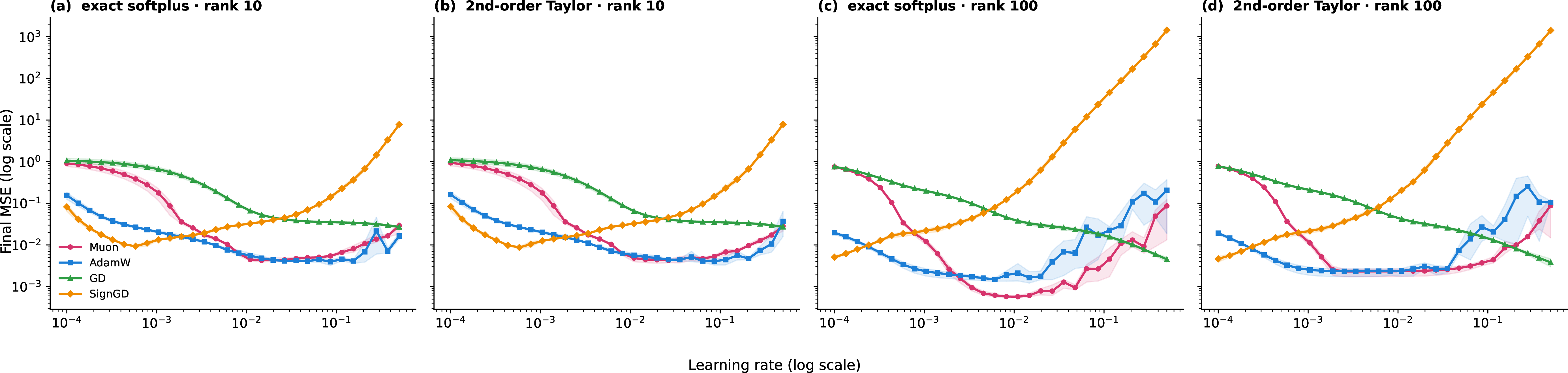
Let \(X\in\mathbb{R}^{N\times d}\) collect the \(N\) inputs. We fit the Gaussian kernel \(K\in\mathbb{R}^{N\times N}\), \(K_{ij}=\exp(-\lVert x_i-x_j\rVert^2/2\sigma^2)\), with the model \(\hat{K}=\phi(XW)\,V^\top\), where \(W\in\mathbb{R}^{d\times R}\), \(V\in\mathbb{R}^{N\times R}\), the search rank \(R\) is the hidden width, and \(\phi\) acts entrywise. This is a nonlinear matrix factorization: for \(\phi=\mathrm{id}\) it collapses to the bilinear low-rank model \(\hat{K}=X(WV^\top)\).
16.0.0.1 Softplus and its expansion.
The softplus \(\phi(z)=\log(1+e^{z})\) has derivative \(\phi'=\sigma\) (the logistic sigmoid). Since \(\sigma-\tfrac12\) is odd, the Maclaurin series of \(\phi\) keeps only the constant, linear, and even-order terms, \[\phi(z)=\log 2+\tfrac12 z+\tfrac18 z^{2}-\tfrac{1}{192}z^{4}+\mathcal{O}(z^{6}).\] The surrogate used in the experiments, \(\tilde{\phi}(z)=\log2+\tfrac12 z+\tfrac18 z^{2}\), is the truncation after the quadratic term (the cubic coefficient vanishes), and is accurate when the pre-activations \(XW\) are small, as enforced by the input scale.
16.0.0.2 The quadratic surrogate is an explicit feature factorization.
With \(A=\tilde{\phi}(XW)\), expanding term by term gives \[\hat{K} = A V^\top = \underbrace{\log2\,\mathbf{1}_{N\times R}V^\top}_{\text{constant }(\mathrm{rank}\le1)} \;+\;\underbrace{\tfrac12\,(XW)V^\top}_{\mathrm{rank}\le\min(R,d)} \;+\;\underbrace{\tfrac18\,(XW)^{\odot 2}V^\top}_{\text{degree-2 lift}},\] where \(\odot\) is the Hadamard product. The linear term is exactly the classical rank-\(R\) bilinear factorization, whose rank is further capped by \(\operatorname{rank}(X)\le d\). The Hadamard-square term injects degree-2 monomial features: each column of \(XW\) lies in the \(\le d\)-dimensional column space \(\operatorname{col}(X)\), so the columns of \((XW)^{\odot 2}\) lie in its symmetric square \(\operatorname{Sym}^2(\operatorname{col}(X))\), of dimension \(\le\binom{d+1}{2}\). Hence the model factorizes \(K\) through the fixed feature set \(\{\mathbf{1}\}\cup\operatorname{col}(X)\cup\operatorname{Sym}^2(\operatorname{col}(X))\), and \[\operatorname{rank}(\hat{K})\;\le\;\min\!\Big(R,\;\tbinom{d+2}{2}\Big). \label{eq:rank-cap}\tag{17}\] The quadratic model therefore cannot exceed rank \(\binom{d+2}{2}\) (\(=21\) for \(d=5\)) no matter how large the search rank \(R\) is.
16.0.0.3 Consequence for the comparison.
Equation equation 17 predicts a sharp regime split, which Fig. 12 confirms. When \(R\le\binom{d+2}{2}\) (here \(R=10\)), the search rank is the binding constraint and the truncation is invisible: exact softplus and its surrogate behave almost identically (panels (a) vs (b)). When \(R>\binom{d+2}{2}\) (here \(R=100\)), the degree-2 cap binds for the surrogate but not for exact softplus, so the exact activation attains a strictly lower error (panel (c) below (d)). In both regimes the activation is a mild perturbation of the same nonlinear-factorization family, while the search rank \(R\) governs how much of the kernel’s polynomial spectrum the model can represent, and, empirically, is what separates the optimizers.
17 Analytical Solutions of the Matrix Factorization for AdamW and Muon↩︎
17.1 Problem Setup↩︎
We consider the Matrix Factorization objective function: \[\mathcal{L}(U, V) = \frac{1}{2} \| U V^T - R \|_F^2,\] where \(U, V \in \mathbb{R}^{N \times r}\). At iteration \(t\), we seek the optimal update step \(\Delta U\) for the factor \(U\) (the derivation for \(V\) is symmetric). Let \(G_t = \nabla_U \mathcal{L} = (U_t V_t^T - R)V_t\) be the gradient at step \(t\).
Since the global optimization is intractable, iterative optimizers solve a local proxy problem at each step. We derive the analytical solution for these proxy problems. Throughout, \(v_t\) (lowercase) denotes the per-coordinate second-moment estimate, with entries \(v_{t,ij}\); this is distinct from the factor \(V_t\).
17.2 The AdamW Analytical Solution↩︎
Under the decoupled–weight-decay approximation of Loshchilov & Hutter (2017), the AdamW update is the analytical solution to minimizing the linearized loss subject to an adaptive Mahalanobis-distance trust region, with weight decay applied as a separate additive step.
17.2.0.1 The Optimization Problem.
We first consider the linearized loss penalized by the local curvature estimated by the diagonal second-moment estimate \(v_t\): \[\Delta U^{\dagger} = \mathop{\mathrm{arg\,min}}_{\Delta U \in \mathbb{R}^{N \times r}} \left( \underbrace{\langle G_t, \Delta U \rangle}_{\text{Linear Descent}} + \underbrace{\frac{1}{2\eta} \sum_{i,j} \sqrt{v_{t,ij}}\, (\Delta U_{ij})^2}_{\text{Adaptive Trust Region}} \right).\]
17.2.0.2 Derivation of the trust-region step.
The objective is separable across coordinates. Taking the derivative with respect to a single entry \(\Delta U_{ij}\) and setting it to zero, \[G_{t,ij} + \frac{1}{\eta} \sqrt{v_{t,ij}}\, \Delta U_{ij} = 0 \quad\Longrightarrow\quad \Delta U^{\dagger}_{ij} = -\,\eta\, \frac{G_{t,ij}}{\sqrt{v_{t,ij}}}.\]
17.2.0.3 Decoupled weight decay.
AdamW then applies weight decay as a separate step that is not passed through the preconditioner: \[\boxed{\;\Delta U^*_{ij} = -\,\eta \left( \frac{G_{t,ij}}{\sqrt{v_{t,ij}}} + \lambda\, U_{t,ij} \right).\;}\]
17.2.0.4 Remark (why decoupling matters).
Had we instead folded the penalty \(\tfrac{\lambda}{2}\|U_t + \Delta U\|_F^2\) directly into the proxy, the exact stationary point would be \[\left( \frac{1}{\eta}\sqrt{v_{t,ij}} + \lambda \right) \Delta U_{ij} = -\big(G_{t,ij} + \lambda U_{t,ij}\big) \;\Longrightarrow\; \Delta U_{ij} = -\,\eta\,\frac{G_{t,ij} + \lambda U_{t,ij}}{\sqrt{v_{t,ij}} + \eta\lambda}.\] This couples the decay to the preconditioner (dividing the decay term by \(\sqrt{v_{t,ij}}\)) and is precisely Adam with \(L_2\) regularization, not AdamW. AdamW is recovered by (i) neglecting \(\eta\lambda\) in the denominator and (ii) decoupling the decay so that \(\lambda U_{t,ij}\) is not rescaled by the curvature. Hence the boxed expression is an approximation, not the exact minimizer of the coupled proxy.
17.2.0.5 Conclusion.
AdamW rescales every coordinate independently based on the diagonal curvature \(\sqrt{v_{t,ij}}\), and adds an unpreconditioned weight-decay term.
17.3 The Muon Analytical Solution↩︎
The Muon update is the exact analytical solution to the Orthogonal Procrustes Problem. It finds the orthonormal-column update direction that aligns maximally with the negative gradient; this direction is the polar factor of \(-G_t\).
17.3.0.1 The Optimization Problem.
We seek the matrix \(O \in \mathbb{R}^{N \times r}\) closest to the negative gradient \(-G_t\), constrained to have orthonormal columns: \[O^* = \mathop{\mathrm{arg\,min}}_{O\,:\,O^T O = I_r} \; \| (-G_t) - O \|_F^2 .\] The update is then \(\Delta U = \eta\, O^*\).
17.3.1 Step-by-Step Derivation↩︎
17.3.1.1 Step 1: Expand the objective.
\[\begin{align} \| -G_t - O \|_F^2 &= \mathop{\mathrm{Tr}}\!\left( (G_t + O)^T (G_t + O) \right) \\ &= \mathop{\mathrm{Tr}}(G_t^T G_t) + \mathop{\mathrm{Tr}}(O^T O) + 2\,\mathop{\mathrm{Tr}}(G_t^T O). \end{align}\] The term \(\mathop{\mathrm{Tr}}(G_t^T G_t)\) is constant, and \(\mathop{\mathrm{Tr}}(O^T O) = \mathop{\mathrm{Tr}}(I_r) = r\) is constant. The cross term carries a plus sign, so minimizing the norm is equivalent to minimizing \(\mathop{\mathrm{Tr}}(G_t^T O)\) , equivalently maximizing the alignment with the negative gradient, \(\mathop{\mathrm{Tr}}\!\big((-G_t)^T O\big)\): \[\min_{O\,:\,O^T O = I_r} \; \mathop{\mathrm{Tr}}(G_t^T O).\]
17.3.1.2 Step 2: Singular Value Decomposition.
Let the (thin) SVD of the gradient be \(G_t = P \Sigma Q^T\), where \(P \in \mathbb{R}^{N \times r}\) has orthonormal columns (\(P^T P = I_r\)), \(\Sigma \in \mathbb{R}^{r \times r}\) is diagonal with singular values \(\sigma_i \ge 0\), and \(Q \in \mathbb{R}^{r \times r}\) is orthogonal. Then \[\mathop{\mathrm{Tr}}(G_t^T O) = \mathop{\mathrm{Tr}}\!\big( Q \Sigma P^T O \big) = \mathop{\mathrm{Tr}}\!\big( \Sigma\, (P^T O Q) \big),\] using the cyclic property of the trace.
17.3.1.3 Step 3: Bound the matrix \(Z\).
Define \(Z = P^T O Q \in \mathbb{R}^{r \times r}\). Each of \(P\), \(O\) has orthonormal columns and \(Q\) is orthogonal, so each is a (semi-)isometry with spectral norm \(1\). Hence \(\sigma_{\max}(Z) \le \|P^T\|_2 \,\|O\|_2 \,\|Q\|_2 = 1\). (Note \(Z\) need not be orthogonal when \(N > r\), since \(O O^T \ne I_N\); we only require the norm bound.) In particular, every diagonal entry satisfies \(|Z_{ii}| \le \sigma_{\max}(Z) \le 1\). The objective becomes \[\mathop{\mathrm{Tr}}(\Sigma Z) = \sum_{i=1}^r \sigma_i Z_{ii}.\]
17.3.1.4 Step 4: Minimize.
Since \(\sigma_i \ge 0\) and \(|Z_{ii}| \le 1\), the sum \(\sum_i \sigma_i Z_{ii}\) is minimized when \(Z_{ii} = -1\) for all \(i\), i.e.\(Z = -I_r\) (attained by the admissible choice \(O = -PQ^T\)). Solving back, \[\begin{align} P^T O Q &= -I_r \\ O^* &= -\,P\,Q^T. \end{align}\] \[\boxed{\;O^* = -\,P Q^T, \qquad \Delta U = \eta\, O^* = -\,\eta\, P Q^T.\;}\] Equivalently, \(O^*\) is the polar factor of the negative gradient \(-G_t\), and the update \(\Delta U = -\eta\,PQ^T\) is a genuine descent step (it removes the singular-value magnitudes of \(G_t\), keeping only its \(PQ^T\) “direction”).
17.3.2 Connection to Newton–Schulz↩︎
The matrix \(P Q^T\) is the polar factor of \(G_t\). Computing the SVD at every step is expensive, so Muon computes \(PQ^T\) via the Newton–Schulz iteration \[X_{k+1} = \frac{1}{2} X_k \big(3I - X_k^T X_k\big), \qquad X_0 = \frac{G_t}{\|G_t\|_2},\] which converges quadratically to \(P Q^T\). The descent update is then \(\Delta U = -\eta\, X_\infty = -\eta\, P Q^T\), consistent with the boxed solution above.
17.4 Implications for Matrix Factorization↩︎
This derivation highlights the fundamental difference in update scaling. Both updates act on matrices in \(\mathbb{R}^{N \times r}\).
17.4.0.1 1. AdamW scaling (dimension dependent).
Assuming active gradients (\(G_{ij}/\sqrt{v_{ij}} \approx \pm 1\)) and negligible weight decay, the squared norm of the update scales with the number of entries \(N \times r\): \[\| \Delta W_{\text{Adam}} \|_F^2 \approx \sum_{i,j} \eta^2 = \eta^2 (N \cdot r).\]
17.4.0.2 2. Muon scaling (rank dependent).
Since \(O^* = -P Q^T\) has orthonormal columns, \((O^*)^T O^* = Q P^T P Q^T = I_r\), so the sign is immaterial to the norm: \[\| \Delta W_{\text{Muon}} \|_F^2 = \eta^2 \,\mathop{\mathrm{Tr}}\!\big( (O^*)^T O^* \big) = \eta^2 \,\mathop{\mathrm{Tr}}(I_r) = \eta^2 r.\]
17.4.0.3 Conclusion.
\[\frac{\| \Delta W_{\text{Adam}} \|_F}{\| \Delta W_{\text{Muon}} \|_F} \approx \sqrt{N}.\] In our experiments with \(N = 1000\), AdamW naturally takes steps \(\approx 31.6\) times larger than Muon for the same learning rate \(\eta\). This explains the necessity of scaling \(\eta_{\text{Muon}} \approx \sqrt{N}\,\cdot\,\eta_{\text{AdamW}}\) to achieve comparable convergence rates.