1 Introduction↩︎

The ability to dynamically perceive, memorize, and reason about 3D environments is a fundamental prerequisite for embodied agents. Recently, 3D Scene Graphs (3DSGs) have emerged as a crucial representation for this purpose, encoding a scene into a graph where nodes denote objects and edges capture their pairwise relationships. Driven by the advent of Vision-Language Models (VLMs), modern 3DSG frameworks have rapidly evolved. Early methods primarily focused on extracting closed-set semantics [1]–[3], limiting agents to predefined categories. Subsequent breakthroughs introduced open-vocabulary concepts [4]–[13], enabling zero-shot querying of novel objects. More recently, the field has progressed toward task-driven [9], [14]–[16] and functional graphs [4], [17]–[19], marking a critical shift toward rethinking the graph construction process and representational structure from the perspective of downstream robotic tasks. Collectively, these advancements provide a powerful structural foundation for comprehensive 3D scene understanding and persistent spatial memory, significantly expanding the boundaries of robot navigation [10], [12], [20]–[24] and manipulation [12], [25]–[27].

However, behind the conventional pursuit of holistic representational fidelity lies a critical conceptual blind spot: existing 3DSG construction pipelines operate on an unconstrained Ahead-of-Time (AOT), “build-everything-then-filter” paradigm. This unyielding fixation on global structural completeness triggers severe observation redundancy and ultimately inflicts a perceptual saturation effect. As empirically exposed by our exploratory motivation experiments (Sec. 3), blindly maximizing global scene graph accuracy does not monotonically translate to superior downstream robotic execution; instead, unconstrained bottom-up over-semanticization severely pollutes the LLM’s cognitive context with semantic noise and introduces unsustainable latencies. Crucially, even contemporary “task-driven” frameworks fail to bypass this bottleneck. Being inherently result-oriented, they merely utilize task queries as retrospective filters or post-hoc structural aggregators, leaving their underlying construction workflows completely blind to resource allocation over the timeline.

Humans, by contrast, are fundamentally immune to such perceptual saturation due to an elegant, resource-conscious gating mechanism. Upon entering an unfamiliar environment, the human brain does not deploy an unconditional, exhaustive bottom-up scanner to compute fine-grained functional affordances of every random object. Instead, the overwhelming influx of sensory data is heavily compressed and logged merely as a lightweight, fuzzy impression in shallow short-term memory, incurring negligible cognitive cost. It is only when a concrete intent emerges (e.g., “pour a glass of water”) that top-down cognitive focus instantly activates specific regions, allocating resource-intensive operations to resolve fine-grained local details strictly where and when required.

Inspired by this cognitive blueprint, we break away from conventional mapping taxonomies to introduce just-in-time (JIT) scene graph growth as an independent, foundational paradigm. Analogous to JIT compilation in software engineering—which completely eschews heavy Ahead-of-Time (AOT) binaries to dynamically compile source code exclusively at runtime execution points—our JIT paradigm conceptualizes mapping from an entirely different dimension: process-oriented resource management over the temporal axis. Rather than treating graph generation as a passive, monotonic accumulation of massive global structures, the JIT paradigm mandates that task-irrelevant environmental details remain completely dormant from the very outset. The transformation from continuous sensory streams to structured graph entities is thus re-engineered into a highly selective, non-linear growth process, authorizing resource deployment exclusively on-demand.

Following this philosophy, we introduce JITOMA (Just-In-Time On-demand Memory Activation), an online, closed-loop 3DSG framework built upon a clean design principle: a robot should not remember everything in full detail—it instantiates only what the task immediately executes. Breaking away from exhaustive accumulation, JITOMA’s frontend leverages a top-down task heatmap to filter continuous video streams, routing minimal keyframes to the backend to maintain a sparse global foundation of low-cost dormant anchors. Upon receiving an implicit command, the backend Large Language Model (LLM) parses the robotic intent to match and awaken specific anchors. Crucially, computationally expensive graph operations—such as dense node captioning and functional relational inference—are strictly restricted within this awakened local subgraph. This JIT execution boundary inherently streamlines task switching: when transitioning to a new command, the cognitive spotlight simply shifts to activate a different set of anchors, while the previously expanded subgraph gracefully hibernates back to its dormant anchor state, freeing up active working memory. By shifting to active on-demand growth, JITOMA resolves the perceptual saturation dilemma, mitigating computational latency and memory footprints.

To rigorously evaluate these dynamic, process-level mapping capabilities—which conventional static retrieval benchmarks completely fail to encapsulate—we introduce JITOMA-Bench (Sec. 5). Built upon continuous real-world trajectories, JITOMA-Bench reformulates 3DSG evaluation into three progressive tiers: foundational grounding (Tier 1), long-horizon temporal dynamics under streaming task sequences (Tier 2), and complex cognitive reasoning targeting functionally implied latent objects (Tier 3). Crucially, alongside retrieval accuracy, JITOMA-Bench monitors multi-dimensional hardware-efficiency metrics—including active graph size, peak memory accumulation, and frame-rate latencies. This dual-faceted evaluation protocol allows us to systematically expose the trade-offs of perceptual saturation and prove JITOMA’s real-time viability.

2 Related Work↩︎

Ahead-of-Time (AOT) Paradigms in 3D Scene Graphs 3D Scene Graphs (3DSGs) have evolved into a core representation for embodied spatial reasoning by organizing dense sensory data into topological nodes and semantic relationships [1], [2]. Early frameworks primarily relied on closed-set object detectors [1]–[3], which recently progressed toward open-vocabulary abstractions utilizing Vision-Language Models (VLMs) to enable zero-shot querying of novel semantics [4]–[13]. To support physical interactions, contemporary works further incorporate hierarchical structures and functional affordances directly into the graph entities [4], [17], [18]. Despite their rich representational utility, these methods share an unyielding, Ahead-of-Time (AOT) construction philosophy. They operate under the implicit assumption of unbounded onboard compute or post-exploration processing, forcing the streaming perception frontend to exhaustively extract high-fidelity features across the entire environment. Crucially, this paradigm enforces a rigid, predefined structural granularity during the perceptual phase, treating all spatial entities uniformly regardless of their relevance to specific downstream tasks. As the exploration horizon expands, this unconditional asset accumulation and undifferentiated processing trigger severe observation redundancy, inducing a crippling perceptual saturation effect before downstream reasoning even initiates.

Result-Oriented vs. Just-In-Time (JIT) To alleviate the overheads of AOT construction, a nascent line of works explores task-driven 3DSGs to condition graph topologies on downstream requirements [9], [17]. However, earlier frameworks are primarily result-oriented; they employ tasks merely as semantic constraints to cluster or filter pre-computed features, leaving the upstream construction process blind to online resource allocation. A recent departure from this paradigm is FOUND-IT [14], which takes an initial step toward just-in-time adaptation by deferring explicit 3D instance extraction until runtime queries are issued, utilizing a keyframe-indexed visual memory layer to adjust target granularity on demand. Despite this progression, FOUND-IT [14] fundamentally decouples the perception phase from active task reasoning, rendering its input frontend entirely unconditioned. In complete alignment with human cognitive mechanics, a truly efficient embodied agent must allow the immediate task intent to proactively govern upstream perception. In contrast, we present a closed-loop JIT framework that unifies task intent, perception, and memory. Instead of merely postponing interpretation, our paradigm establishes task queries as active runtime controllers that modulate the streaming perception frontend via top-down attention, eliminating observation redundancy at its architectural root while dynamically growing and distilling the subgraph strictly on-demand.

3 Preliminary Findings and Motivation Experiments↩︎

To motivate our Just-In-Time (JIT) on-demand growth framework, we empirically investigate the bottlenecks of AOT, build-then-filter 3D scene graph paradigms through diagnostic pilot studies.

3.1 Does Global Structural Completeness Overwhelm Downstream Reasoners?↩︎

Chasing exhaustive global representational accuracy under tight embodied constraints often conflicts with downstream cognitive efficiency. To isolate this bottleneck, we conduct a diagnostic pilot study aligned with Tier 3 of JITOMA-Bench (Sec. 5), evaluating a Large Language Model (Qwen-3.5-9b [28]) planner on the command: “pack my eyeglasses for travel” within a cluttered real-world cubicle (full specifications in Appendix 8.1). We compare two distinct upstream mapping paradigms: 1.AOT Full Graph: The planner receives a holistic 3D scene graph containing all \(18\) environmental entities unconditionally mapped by a task-agnostic pipeline. 2.JIT Subgraph (Ours): The planner receives a subgraph from just-in-time growth, containing exclusively the \(3\) task-relevant entities (eyeglasses, glasses case, and backpacks) instantiated strictly on-demand.

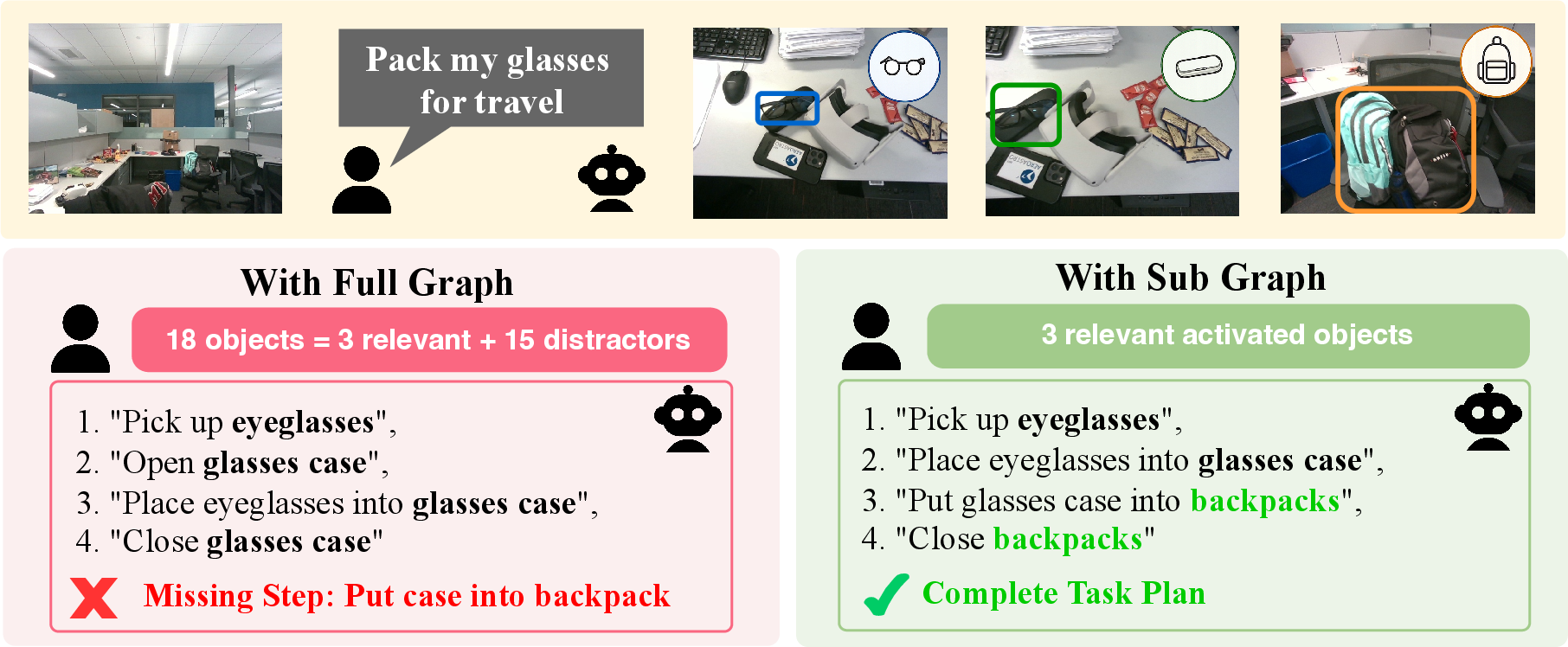
Crucially, the brute-force density of the AOT graph triggers a severe perceptual saturation effect, causing the reasoning engine to suffer from cognitive myopia. Flooded by \(15\) pieces of irrelevant environmental clutter (e.g., hardware drills, mudstone rocks), the model fails to complete the full multi-step spatial-functional dependency chain (Fig.  1). It terminates the plan prematurely after resolving the immediate protective constraint (glasses case), completely omitting the final travel containment step into the backpacks. Conversely, supplied with our sparse JIT foundation, the identical model seamlessly produces a complete execution sequence, confirming that unconstrained bottom-up accuracy paradoxically degrades robotic success.

4 Method↩︎

4.1 Problem Formulation and Architecture Overview↩︎

JITOMA targets online 3D scene graph construction under long-horizon embodied execution, where conventional Ahead-of-Time (AOT) pipelines suffer from perceptual saturation: they exhaustively instantiate global semantic structures before knowing which parts of the scene will actually be used. Given a continuous RGB-D stream and camera poses \(\{(I_t, D_t, P_t)\}_{t=1}^T\), our goal is not to build a complete semantic graph and filter it afterwards. Instead, JITOMA treats graph construction as a just-in-time growth process: the system maintains a sparse, low-cost memory foundation during exploration, while expensive computation is triggered only when a robotic intent requires it.

Formally, at time \(t\), JITOMA maintains a two-tier memory state \[\mathcal{M}_t = \big(V_t^{\mathrm{eph}}, V_t^{\mathrm{anc}}\big),\] where \(V_t^{\mathrm{eph}}\) denotes ephemeral short-term hypotheses and \(V_t^{\mathrm{anc}}\) denotes long-lived dormant anchors. Ephemeral hypotheses store transient, weakly consolidated observations, while dormant anchors serve as stable but intentionally under-specified visual impressions of the environment. Each dormant anchor preserves object existence, coarse geometry, representative crops, and a lightweight visual embedding, but does not initially store dense captions or functional subnodes.

When a natural-language command \(q\) arrives, JITOMA retrieves a subset \(V^{\mathrm{act}}(q) \subseteq V^{\mathrm{anc}}\) from the current dormant anchors. Only these anchors trigger expensive semantic computation. The activated object nodes are then grown into task-specific functional subnodes \(V^{\mathrm{part}}(q)\), yielding \[G^+(q) = \Big( V^{\mathrm{act}}(q) \cup V^{\mathrm{part}}(q), E^{\mathrm{part}}(q) \Big),\] where \(E^{\mathrm{part}}(q)\) connects each activated object to its functional subnode. After execution, reusable captions and functional subnodes are distilled into the corresponding dormant anchors, while other temporary JIT products are discarded. In this way, graph complexity scales with active cognitive demand rather than monotonically with exploration time.

4.2 Intent Parsing and Frontend Just-In-Time Perception↩︎

A key distinction between JITOMA and result-oriented task-driven 3D scene graph methods is that the task does not merely filter a pre-built graph at query time. Instead, the task controls which observations are written into memory during perception. Upon receiving a command \(q\), an LLM-based parser extracts a structured concept set \(C(q) = C_{\mathrm{pri}}(q) \cup C_{\mathrm{lat}}(q)\), where \(C_{\mathrm{pri}}(q)\) contains primary objects explicitly grounded in the command and \(C_{\mathrm{lat}}(q)\) contains latent objects, tools, containers, supports, sources, or destinations required to complete the task. For example in Fig. 2 (a), the command “clean the cup” yields \(C_{\mathrm{pri}}(q)=\{\text{cup}\}\) and infers \(C_{\mathrm{lat}}(q)=\{\text{water faucet}, \text{sponge}\}\).

At timestamp \(t\), a class-agnostic segmentation tracker [29] processes the raw input into tracks \(O_t = \{o_{t,i}\}_{i=1}^{N_t}\), where each track packet is \(o_{t,i}=(M_{t,i},x_{t,i},g_{t,i})\). Here, \(M_{t,i}\) is a 2D mask, \(x_{t,i}\) is an image crop, and \(g_{t,i}\) is coarse 3D geometry. JITOMA deliberately avoids semantic labeling at this stage. To implement just-in-time observation gating, the parsed concepts \(C(q)\) are passed to a vision-language alignment model [30] to produce a task heatmap \(H_t^q\) over the current image, as shown in Fig. 2 (b). The relevance score and selected observations are \[\begin{align} s_{t,i}^{\mathrm{obs}}(q) &= \operatorname{Pool}\big(H_t^q \odot M_{t,i}\big),\\ \widetilde{O}_t(q) &= \operatorname{TopK}_{o_{t,i}\in O_t} s_{t,i}^{\mathrm{obs}}(q). \end{align}\] Only observations in \(\widetilde{O}_t(q)\) are admitted into the ephemeral memory. In this way, the command acts before memory commitment, suppressing redundant observations at the architectural source rather than relying on post-hoc graph filtering.

4.2.0.1 Task-Free Conservative Writing.

When no task is active, JITOMA enters a conservative writing mode. The frontend admits newly observed tracks, but throttles repeated observations of already known regions. A previously observed track is written again only if it contributes a sufficiently novel viewpoint or improves the geometric estimate of an existing anchor. This preserves a global foundation for future queries while avoiding the over-accumulation characteristic of AOT pipelines.

4.3 Dormant Memory Foundation↩︎

JITOMA separates long-term spatial awareness from active semantic reasoning. Rather than maintaining a global graph whose nodes are always semantically expanded, the system uses a two-stage memory foundation composed of ephemeral hypotheses and dormant anchors, as shown in Fig. 2 (c).

4.3.0.1 Ephemeral Hypotheses.

The observations admitted by the frontend first enter \(V_t^{\mathrm{eph}}\) as ephemeral hypotheses. These nodes serve as short-term buffers. An ephemeral hypothesis accumulates lightweight geometric and visual evidence over a local temporal window but remains semantically dormant. Hypotheses that fail stability checks are discarded as forgotten short-term memory.

4.3.0.2 Dormant Anchors.

When an ephemeral hypothesis \(v_j \in V_t^{\mathrm{eph}}\) satisfies the stability check, it is promoted into a dormant anchor \(v_j \in V_t^{\mathrm{anc}}\). During promotion, JITOMA selects a representative crop \(\bar{x}_j\) from its crop buffer and computes a lightweight visual key: \(z_j = \operatorname{CLIP}_{\mathrm{img}}(\bar{x}_j).\) This embedding is the main distinction between ephemeral hypotheses and dormant anchors: it enables future query-time retrieval without dense semantic expansion. The anchor remains semantically dormant, storing only low-cost geometry, representative crops, and the CLIP embedding \(z_j\). Dense captions and functional subnodes are computed only after task activation. Thus, global memory grows as a sparse set of stable visual impressions rather than a fully expanded semantic graph.

4.4 On-Demand Memory Activation↩︎

When a command \(q\) arrives, JITOMA activates memory through a two-stage just-in-time retrieval process, as shown in Fig. 2 (c). For readability, we omit the time subscript in this subsection and operate on the current dormant anchor set \(V^{\mathrm{anc}}\). For each parsed concept \(c \in C(q)\), JITOMA first ranks dormant anchors with lightweight keys and retrieves three candidates: \[\begin{align} s_j^{\mathrm{ret}}(c) &= \cos\big( \operatorname{CLIP}_{\mathrm{text}}(c), z_j \big) + \lambda \tilde{h}_j^c,\\ B(c) &= \operatorname{Top3}_{v_j\in V^{\mathrm{anc}}} s_j^{\mathrm{ret}}(c). \end{align}\] Here, \(z_j\) is the CLIP visual key of anchor \(v_j\), and \(\tilde{h}_j^c\) records accumulated task-heatmap evidence from the frontend. Only anchors in \(B(c)\) are allowed to invoke expensive semantic processing; all other anchors remain dormant. Given the representative crops of the retrieved candidates, JITOMA performs batched DAM captioning [29], [31]: \[\{d_j\}_{v_j\in B(c)} = \operatorname{DAM}_{\mathrm{cap}} \big(\{\bar{x}_j\}_{v_j\in B(c)}\big).\] The command, concept, and candidate-caption pairs are then passed to an LLM reranker. The selected anchors and the resulting activated set are \[\begin{align} v^*(c) &= \operatorname{LLM}_{\mathrm{rerank}} \big(q,c,\{(v_j,d_j)\}_{v_j\in B(c)}\big),\\ V^{\mathrm{act}}(q) &= \{v^*(c)\mid c\in C(q)\} \subseteq V^{\mathrm{anc}}. \end{align}\] The reranker activates one anchor for each concept; all unselected candidates return to the dormant state. This is the core just-in-time mechanism: JITOMA spends captioning and LLM reasoning only on a few retrieved candidates, while all other memory remains dormant.

4.5 Task-Conditioned Subgraph Growth↩︎

After on-demand activation, \(V^{\mathrm{act}}(q)\) contains the primary and latent objects required by the command. The remaining goal is to grow these activated objects into functional graph nodes. For each activated anchor \(v_j \in V^{\mathrm{act}}(q)\), JITOMA provides its crop \(\bar{x}_j\), the command \(q\), and its object caption \(d_j\) to a VLM. The predicted interactive part, its 2D grounding, and its 3D bounding box are \[\begin{align} \ell_j^q &= \operatorname{VLM}_{\mathrm{part}} \big(q,\bar{x}_j,d_j\big),\\ m_j^q &= \operatorname{Seg} \big(\bar{x}_j,\ell_j^q\big),\\ b_j^q &= \operatorname{OBB} \big(\Pi^{-1}(m_j^q,D_j,P_j)\big). \end{align}\] Here, \(\ell_j^q\) is a textual description of the task-relevant functional part, \(\operatorname{Seg}\) denotes heatmap-based mask grounding, and \(\Pi^{-1}\) back-projects the mask using the depth \(D_j\) and camera pose \(P_j\).

Each localized part becomes a functional subnode attached to its object anchor: \[\begin{align} p_j^q &= (b_j^q,\ell_j^q),\\ V^{\mathrm{part}}(q) &= \{p_j^q\mid v_j\in V^{\mathrm{act}}(q)\},\\ E^{\mathrm{part}}(q) &= \{(v_j,p_j^q)\mid v_j\in V^{\mathrm{act}}(q)\}. \end{align}\] The final just-in-time grown subgraph is therefore \[G^+(q) = \Big( V^{\mathrm{act}}(q)\cup V^{\mathrm{part}}(q), E^{\mathrm{part}}(q) \Big).\] Thus, JITOMA grows the graph only where execution requires fine-grained interaction, rather than expanding all objects into dense structures ahead of time.

4.6 Subgraph Distillation and Operating Modes↩︎

After the grown subgraph \(G^+(q)\) is used for execution, JITOMA collapses the active query overlay. Expensive but reusable products, including object captions and functional subnodes, are distilled as dormant auxiliary attributes of the corresponding anchors: \[\mathcal{A}_j \leftarrow \mathcal{A}_j\cup\{d_j,p_j^q\}, \qquad v_j\in V^{\mathrm{act}}(q),\] where \(\mathcal{A}_j\) denotes the reusable auxiliary attributes of anchor \(v_j\). Other JIT byproducts, such as heatmaps, masks, reranking candidates, temporary edges, and active overlays, are discarded. The distilled information is reused only when a future query reactivates the anchor.

As shown in Fig. 2 (d), JITOMA operates in three modes. With no query, it only writes observations and promotes stable anchors. With a single query, it activates relevant anchors, grows \(G^+(q)\), distills reusable outputs, and collapses after execution. With concurrent queries, multiple active overlays share the same dormant anchor foundation while keeping their temporary semantics separate.

5 Dataset and Benchmark↩︎

Clio-Bench [9] provides real-world RGB-D trajectories and geometric ground truth for evaluating real-time, task-driven open-set 3DSGs. However, Clio-Bench and other existing benchmarks leave three important gaps: (G1) Peak Resource Dynamics, because final graph statistics do not reveal the peak graph size and computation incurred throughout online construction; (G2) Long-Horizon Multi-Tasking, because evaluation focuses on isolated atomic tasks rather than a sequence of task switches within the same continuous scene; and (G3) Complex Intent Grounding, because existing commands typically specify one target object explicitly, while realistic instructions may require multiple primary and latent objects. To address these, we introduce JITOMA-Bench, which retains Clio’s three scenes and introduces a three-tier evaluation of single-query grounding, streaming multi-task adaptation, and complex Primary–Latent intent grounding, as detailed in Sec. 5.1.

5.1 Task Annotations and Complementary Evaluation Tracks↩︎

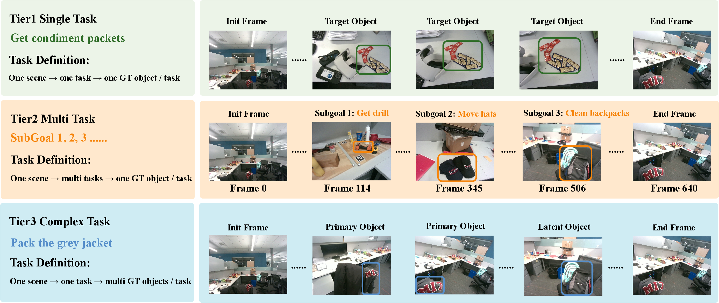
Tier 1: Foundational Grounding. As shown in Fig. 3, Tier 1 evaluates each explicit single-GT task independently, providing a controlled measure of conventional 3DSG object grounding.

Tier 2: Long-Horizon Dynamics. Tier 2 addresses G2 by evaluating continual adaptation under an evolving task stream within the same scene. To construct potentially overlapping tasks, we manually annotate the first- and last-visible frames of each target (e.g., Frame X for Subgoal x in Fig. 3). Each task is activated at its first-visible frame and evaluated ten frames after its last-visible frame.

Tier 3: Complex Cognitive Reasoning. Tier 3 addresses G3 by evaluating complex instructions that require multiple explicit and latent objects, while following the Tier 1 timing protocol. Using the Clio ground-truth labels, GPT-5.4 [32] generated 23, 15, and 18 candidate tasks for the Apartment, Office, and Cubicle scenes, respectively, by composing single-object tasks into complex instructions. The authors assigned primary and latent objects using the corresponding Clio labels, after which three PhD researchers independently reviewed each instruction and assignment. A candidate was removed if at least two reviewers judged that (i) the task–object set was ambiguous, (ii) the task was infeasible or unreasonable, or (iii) any annotated latent object was unnecessary for task completion.

5.2 Evaluation Metrics↩︎

Our evaluation follows two complementary objectives: grounding accuracy and system efficiency. For accuracy, we report the top-1 Intersection over Union (IoU), averaged across queries, to measure geometric agreement between the retrieved object and its ground truth. We further define mR@K as the arithmetic mean of Recall@K over IoU thresholds \(\{0.1, 0.2, 0.3\}\), capturing both semantic retrieval and localization robustness. In Tier 3, Primary and Latent concepts are evaluated separately before being averaged within each task, ensuring that performance reflects both explicit-object grounding and implicit-intent understanding.

For efficiency, we track three critical indicators to characterize representation scalability and online processing cost. Objs measures the global object-node count maintained when tasks are evaluated at the exact moment of answering the query, quantifying the computational cost during task processing. Peak captures the maximum active object-node count over the entire scene replay, exposing transient representation overhead and worst-case computational workload that endpoint-only metrics may conceal. Finally, TPF (Time Per Frame) measures the average end-to-end processing time (in seconds) per processed frame, characterizing system-level efficiency for online scene understanding.

6 Experiments↩︎

To evaluate JITOMA’s just-in-time, on-demand paradigm, we conduct experiments on JITOMA-Bench. Our evaluation is designed to answer three core questions: (Q1) Can JITOMA mitigate perceptual saturation and improve task grounding across increasing reasoning complexity? (Q2) Can JITOMA bound active graph size and peak memory during long-horizon sequential task execution? (Q3) Does just-in-time activation preserve real-time streaming performance.

6.1 Experimental Setup↩︎

Baselines. We benchmark JITOMA against three representative state-of-the-art frameworks: ConceptGraphs [5], a foundational bottom-up method that builds a global semantic graph by exhaustively aggregating object-level captions; ReasoningGraph [33], an enhanced hierarchical mapping approach that integrates open-vocabulary features for object-relational reasoning; and Clio [9], a real-time task-driven scene graph that clusters and retrieves task-relevant objects based on queries.

Implementation Details. We implement JITOMA using Qwen3.5-9b [28] as the foundation model, paired with DAM [31] in batch [29] for on-demand captioning. To ensure a fair comparison, all methods, including JITOMA and the baselines, are evaluated on the NVIDIA RTX A6000 GPU, utilizing the identical sensory streams and task queries provided by JITOMA-Bench.

6.2 Main Results: Accuracy and System Efficiency↩︎

We report performance across the three tiers of JITOMA-Bench in Table ¿tbl:tab:main95results?. The evaluation jointly measures grounding accuracy using IoU, mR@1, and mR@3, and system efficiency using the active object count (Objs), peak active graph size (Peak), and per-frame processing time (TPF).

Grounding accuracy and cross-tier robustness (Q1). JITOMA achieves strong grounding accuracy across all three evaluation tiers. On Tier 1, it obtains the best mR@1 and mR@3 in all three scenes, as well as the best IoU in Apartment and Office. More importantly, performance does not degrade when moving from isolated tasks in Tier 1 to the long-horizon task stream in Tier 2. Across the three scenes, all nine accuracy entries improve, with average gains of 5.0 IoU, 9.4 mR@1, and 7.3 mR@3. This improvement is achieved while keeping the number of active objects unchanged and the active peak bounded at four, demonstrating robust grounding under continual task switching rather than only on independently evaluated queries.

The advantage becomes most evident on Tier 3, where each instruction involves multiple primary and latent objects. JITOMA achieves the highest IoU, mR@1, and mR@3 in every scene, even when the baselines are augmented with our task parser. The substantial gap between the vanilla and augmented baseline results confirms that intent parsing is an important bottleneck. However, JITOMA’s consistent advantage over the augmented variants shows that its gains also arise from activating a compact and explicit task-relevant representation, rather than from task parsing alone.

Bounded active graph dynamics (Q2). JITOMA decouples the accumulated memory size from the amount of graph structure actively processed by the current task. In the Peak column, the value outside parentheses denotes the maximum number of simultaneously active nodes, while the parenthesized value denotes dormant anchors retained in the lightweight memory foundation. These dormant anchors store low-cost geometry, visual crops, and CLIP keys, but do not trigger expensive captioning or functional subnode generation unless reactivated.

Across Tier 1 and Tier 2, JITOMA maintains only one or two objects at query time and an active peak of at most four, despite retaining 284–512 dormant anchors. Notably, the active peak remains at four or below from Tier 1 to Tier 2 in all scenes, changing by at most one node despite the continuous stream of task switches. Tier 3 raises the active graph to six objects and a peak of twelve, reflecting the larger number of primary, latent, and functional nodes required by complex instructions. In contrast, existing methods maintain hundreds or thousands of active nodes. These results show that JITOMA scales expensive graph computation with current cognitive demand, rather than with the total amount of explored scene content.

Latency versus semantic richness (Q3). JITOMA is not designed to minimize TPF through lightweight embedding matching alone. Unlike methods that primarily rely on CLIP-style similarity, JITOMA deliberately performs batched DAM captioning and grows explicit functional subnodes for the activated objects. This introduces unavoidable additional latency, but provides richer scene information, including explicit object descriptions and localized, actionable 3D interaction parts.

Despite these additional operations, JITOMA maintains a stable TPF of 0.56–0.63 s across all scenes and tiers. When moving from Tier 1 to the long-horizon Tier 2 setting, its TPF increases by only 0.01–0.02 s per frame, showing that repeated task switching does not cause cumulative processing overhead. On Tier 2, JITOMA remains within 0.08 s per frame of Clio in all scenes and is faster in Cubicle, while providing substantially richer explicit semantics. It is also approximately 9–21\(\times\) faster than the caption-heavy ConceptGraphs baseline on Tier 2. Although ReasoningGraph reports a lower raw TPF, it retains hundreds to thousands of active nodes and performs substantially worse on complex Tier 3 grounding. Overall, JITOMA provides a favorable trade-off: it incurs modest captioning overhead to produce explicit, actionable scene representations, while its just-in-time design confines expensive semantic processing to task-relevant memory and keeps both active graph size and cross-tier latency tightly bounded.

7 Conclusion↩︎

We introduced just-in-time scene graph growth as an alternative to the conventional Ahead-of-Time paradigm, addressing the perceptual saturation caused by exhaustive semantic accumulation. Our framework, JITOMA, maintains a lightweight foundation of dormant anchors, uses task intent to gate streaming observations, and activates expensive captioning and functional subgraph growth only for memory relevant to the current command. Reusable semantic products are distilled back into dormant memory, while temporary query-time structures are discarded, allowing active graph complexity to follow cognitive demand rather than exploration length.

We further introduced JITOMA-Bench to evaluate 3D scene graphs across explicit grounding, long-horizon task switching, and complex instructions involving primary and latent objects. Experiments demonstrate that JITOMA preserves strong grounding accuracy as task complexity increases, keeps active graph size bounded across sequential tasks, and maintains stable cross-tier latency despite producing richer, actionable scene representations. Together, these results suggest that efficient embodied scene understanding should optimize not only what a scene graph represents, but also when and where its semantic structure is instantiated.

8 Experiment↩︎

8.1 Motivation Experiment: Ahead-of-Time (AOT) Full Graph Prompt↩︎

This prompt template is utilized in our exploratory motivation experiment (Sec. 3) to evaluate downstream Large Language Model (LLM) task planning performance when exposed to the conventional Ahead-of-Time (AOT) mapping paradigm. By inundating the cognitive context window with the complete, unconstrained set of all 18 tracked environmental objects, this setup systematically exposes the cognitive agent to extreme observation redundancy, thereby inducing and evaluating the perceptual saturation effect under real-world clutter.

8.2 Motivation Experiment: Just-In-Time (JIT) Subgraph Prompt↩︎

This prompt template corresponds directly to our proposed Just-In-Time (JIT) mapping paradigm operationalized in JITOMA. Instead of compiling an unconstrained global structure, the input scene graph undergoes process-level resource gating. Computational overhead and semantic binding are dynamically deployed on-demand, restricting the active graph to exclusively encapsulate the task-relevant local subgraph.

References↩︎