MSC 2020: 05C45 (primary); 05B20, 05C38, 05B35, 52B05 (secondary). Keywords: interchange graph, (0,1)-matrix, Hamilton-connected, Hamilton-laceable, disjoint path cover, transportation polytope, combinatorial Gray code.

Let \(R=(r_1,\dots,r_m)\) and \(S=(s_1,\dots,s_n)\) be nonnegative integer vectors with \(\sum r_i=\sum s_j\), and let \(\mathcal{A}(R,S)\) be the set of \(m\times n\) \((0,1)\)-matrices with row sums \(R\) and column sums \(S\). A \(2\times 2\) interchange replaces a submatrix \(\left[\begin{smallmatrix}1&0\\0&1\end{smallmatrix}\right]\) by \(\left[\begin{smallmatrix}0&1\\1&0\end{smallmatrix}\right]\), or vice versa, leaving all other entries fixed. Ryser’s classical theorem [1] states that any two members of \(\mathcal{A}(R,S)\) are connected by a sequence of interchanges. The interchange graph \(G(R,S)\) records this: its vertices are the matrices of \(\mathcal{A}(R,S)\), and two are adjacent precisely when one is obtained from the other by a single interchange. Interchange graphs are central objects of combinatorial matrix theory; they are spanning subgraphs of the \(1\)-skeleta of transportation polytopes (every interchange is a polytope edge, though the skeleton has further edges, along longer alternating cycles), and they are the state graphs of the standard swap Markov chains on contingency tables.

Brualdi [2] conjectured the following.

The conjecture is known only in special cases. Hamilton cycles were obtained for certain special margin vectors by Zhang–Zhang and H. Zhang (see Brualdi [3] for an account). Li and Zhang [4] Thm. 2.3, pp. 109–110 proved Hamiltonicity when one margin is all-ones (equivalently, by complementation, all-\((\max-1)\)). In the paragraph following that proof they state that the same method gives edge-Hamiltonicity [4, p. 110]. This class consists of labeled set partitions with prescribed part sizes and is more general than the permutation-margin case; the complete transposition graph occurs only when both margins are all-ones. Arikati and Peled [5] gave the exact split-graph translation of a bipartite realization graph described below, and established Hamiltonicity for degree sequences of majorization gap one. This realization-graph viewpoint is surveyed by Barrus [6], where the general Hamiltonicity question is likewise recorded as open. The general conjecture has remained open; it appears as Problem P60 in Mütze’s survey [7].

We establish a strengthening. Recall that a connected graph is Hamilton-connected if every pair of distinct vertices is joined by a Hamilton path, and that a connected bipartite graph is Hamilton-laceable if every pair of vertices in different color classes is joined by a Hamilton path (for a bipartite graph the latter is the strongest possible such property). Call a graph maximally Hamiltonian if it is Hamilton-laceable when bipartite and Hamilton-connected when not, a dichotomy with precedent in Chen and Quimpo’s work on abelian group graphs [8].

Maximal Hamiltonicity, rather than bare Hamiltonicity, is the property our induction can carry: a Hamilton cycle is not preserved under the Cartesian-product and fiber gluings that organize the argument, whereas Hamilton-connectedness and -laceability are. For a graph of order at least three, take any edge, join its endpoints by the Hamilton path supplied by maximal Hamiltonicity, and close with that edge. Thus every edge lies on a Hamilton cycle. The two-vertex interchange graph is \(K_2\); its sole edge gives the two-term cyclic listing, although \(K_2\) is not a cycle under the standard simple-graph convention. The one-vertex class is maximally Hamiltonian only vacuously and has no Hamilton cycle under that convention. Accordingly, a statement of Brualdi’s conjecture that includes the singleton must either exclude it from the Hamilton-cycle conclusion or declare its one-term listing to be a degenerate cycle. The Lean companion also covers the empty class vacuously, so its statement is formally stronger than the display above.

Proof. A \((0,1)\)-matrix with margins \(R,S\) is the biadjacency matrix of a labeled bipartite graph on fixed sides \(X=\{x_1,\ldots,x_m\}\) and \(Y=\{y_1,\ldots,y_n\}\), and an interchange is exactly a color-class-preserving \(2\)-switch. This identifies its bipartite realization graph with \(G(R,S)\).

For the split correspondence, add every edge inside \(X\) and no edge inside \(Y\). A bipartite realization with side degrees \(R=(r_i)\) and \(S=(s_j)\) becomes a split realization on the labeled partition \(X\mathbin{\dot{\cup}}Y\) with degree sequence \[d_{R,S}=(m-1+r_1,\ldots,m-1+r_m,s_1,\ldots,s_n).\] Deleting the fixed clique edges reverses the map. A \(2\)-switch in a split realization preserves its clique–independent-set partition, and it is precisely a bipartite \(2\)-switch after the clique edges are deleted. Arikati and Peled observe that connectivity of the realization graph makes this a bijection onto all labeled realizations of \(d_{R,S}\), hence an isomorphism of realization graphs [5]. Conversely, choose the labeled clique \(X\) and independent set \(Y\) of a split sequence \(d\); subtract \(m-1\) from the degrees on \(X\) and retain the degrees on \(Y\) to recover \((R,S)\) and the inverse isomorphism. Theorem 1.1 now applies in both directions. \(\square\)

Outline. Section 2 fixes notation and recalls the structure theory of interchange graphs. The proof of Theorem 1.1 is a structural induction on the number of matrices in the class; Section 3 lays out its architecture. The primary split is on whether \(G(R,S)\) is bipartite.

A bipartite class is a Cartesian product of complete transposition graphs (Proposition 2.2), and we settle every such class at once, without induction, through the following paired-cover property.

Here a balanced bipartite interchange graph is one that is bipartite with color classes of equal size; the paired-disjoint-path-cover property is defined in Section 2.4. A paired cover yields a Hamilton path between any two opposite-colored vertices, so the Bipartite 2-DPC Lemma gives Hamilton-laceability for the whole bipartite branch. Section 7 proves it: by a classical theorem of Brualdi every balanced bipartite interchange graph is a Cartesian product of complete transposition graphs, and a double induction built on the Coleman–Fischberg–Gong–Harrington–Wong theorem shows every such product is paired \(2\)-disjoint-path-coverable.

A non-bipartite class is treated by the induction and shown Hamilton-connected. After deleting inactive lines, a surviving invariant position (Section 2.2) expresses the class as a nontrivial Cartesian product of smaller interchange graphs, and Section 4 lifts maximal Hamiltonicity from the factors. A class with no invariant position is prime: its base cases, the Johnson graphs and the classes of order at most six, are handled in Section 6, and the remaining large prime classes by the pivot-and-fiber construction of Section 5, whose line quotients are matroid base-exchange graphs. The Bipartite 2-DPC Lemma returns as a subroutine inside Section 4 whenever a non-bipartite product has a bipartite factor.

Verification. The argument has been checked twice by machine, in complementary ways. First, the entire proof (the reduction of Sections 3–6, including the pivot construction of Section 5, and the double induction of Section 7) has been formalized in the Lean 4 proof assistant. The composed statement, that every interchange graph is maximally Hamiltonian, is machine-checked from Lean’s foundations together with exactly seven axioms. Six are statements of cited theorems of the refereed literature — the results of Ryser, Brualdi, Brualdi–Manber, Naddef–Pulleyblank, and Alspach quoted in Sections 1–2 and 5–6 — and the seventh records a classical transportation-polytope dimension count, printed as [3, Sec. 9.13] after Brualdi, Hartfiel, and Hwang; the sources’ standing nonemptiness conventions are made explicit. The results of Coleman et al. that Section 7 imports — Theorem 7.2 ([9]) with its Proposition 1.6, the down-closure of paired covers (their Prop. 1.1(c), Theorem 7.3 here), and the paired hypercube covers of [10] — are all proved within the formalization from first principles, so those citations record provenance rather than assumption. No other assumption remains, and the axiom trace is mechanically reproducible. The checkable release artifact is the companion repository’s release/paper1 branch. Its public entry point, brualdi_lean/TRUST_SURFACE.md, gives the final theorem declarations, the complete axiom trace, a prose-to-Lean theorem map, the exact statements and source locators for the seven assumed theorems, and the trust boundary. The branch includes lean-toolchain, lakefile.toml, and lake-manifest.json. From the repository root the build gate is

cd brualdi_lean
lake build
test -f .lake/build/lib/lean/BrualdiLean/Sec5.olean
lake env lean CheckAxioms.lean

where CheckAxioms.lean contains importBrualdiLean.Ledger and #printaxiomsBrualdi.Ledger.brualdi_MH; the expected trace is printed verbatim in the public trust surface. The internal label CORE denotes the Bipartite 2-DPC implication represented by Lemma 1.2, and Brualdi-MH denotes the final maximal-Hamiltonicity theorem. These are formal-project labels, not additional mathematical hypotheses. The companion’s proofs are the arguments printed here; an adversarial correspondence audit confirmed the match claim by claim, and the lemma-by-lemma record is summarized in Section 8. Second, the theorem was confirmed on all small classes by an exhaustive SAT-based computation (Section 8). Neither check replaces the cited results, which are used as published. The human-readable proof of Sections 3–7 stands on its own; the mechanization and the SAT sweep corroborate it independently rather than form part of it.

Throughout, \(G(R,S)\) denotes the interchange graph of \(\mathcal{A}(R,S)\), \(\square\) the Cartesian product of graphs, and \(\chi\) the interchange-parity \(2\)-coloring of a bipartite class (Section 2.3). The two normalizations that recur, deleting inactive lines and splitting invariant positions, are collected in Section 2.2.

A line of a matrix is a row or a column; its pattern is its support, the set of positions in which it carries a \(1\). Fix a line \(L\). For each realizable pattern \(p\) of \(L\), the fiber \(F_p\) is the set of matrices of \(\mathcal{A}(R,S)\) whose line \(L\) equals \(p\); the fibers partition \(\mathcal{A}(R,S)\) according to the value of \(L\). All matrices in a fiber share the same \(L\), so a single \(2\times2\) interchange joins two of them only when it avoids \(L\) entirely (an interchange meeting \(L\) would change its pattern, moving to a different fiber). Deleting the common line \(L\) therefore identifies \(F_p\) with the interchange graph of the smaller class on the remaining lines (the residual class obtained by removing \(L\) and reducing the margins by \(p\)). The interchanges that do meet \(L\) pass between fibers and are recorded by the quotient \(Q_L\): its vertices are the realizable patterns of \(L\), with \(p,q\) adjacent when a single interchange (necessarily meeting \(L\)) carries a matrix of \(F_p\) to one of \(F_q\); equivalently, when \(q\) is obtained from \(p\) by relocating one entry of \(L\).

A cell is invariant if it takes the same value in every matrix of \(\mathcal{A}(R,S)\); such a cell is incident to no interchange.

Invariant positions arise in two ways, which must be separated. An inactive line (a row or column whose sum is \(0\) or maximal) consists entirely of constant cells; iteratively deleting inactive lines until none remain leaves a class with the same interchange graph in which every line is active (\(0<r_i<n\) and \(0<s_j<m\)). We assume throughout that the class is active; this deletion is graph-isomorphic, not a factorization. For a class with active lines, the remaining invariant positions induce a genuine Cartesian factorization: after permuting rows and columns, the non-invariant cells occupy disjoint diagonal blocks, every off-diagonal rectangle forced to all-ones or all-zeros, and the matrices vary independently within the blocks. Brualdi’s display identifies the class with the product of the block classes and the interchange graph with the Cartesian product of their interchange graphs [3, Sec. 6.1], pp. 285–286. The same construction appears in Brualdi–Manber: their Theorem 1 gives the invariant block form, and the paragraph following it identifies the two graph factors [11] Thm. 1 and following paragraph, pp. 158–159. Thus every factor is itself the interchange graph of a matrix block, not merely an abstract Sabidussi factor. In an active class both displayed factors have at least two vertices [11]; consequently each has order strictly smaller than their product. Brualdi–Manber’s Theorem 9 gives the converse and the exact prime criterion [11] Thm. 9, p. 169: an active class is prime (admits no nontrivial Cartesian factorization) exactly when it has no invariant positions. We call such a class invariant-free. (Primeness here means Cartesian-indecomposability, not connectivity: \(C_4=K_2\,\square\,K_2\) is connected yet decomposable.) Thus, once inactive lines are deleted, every interchange graph is a Cartesian product of invariant-free (prime) factors: the reduction of Section 3 splits this product off first (Section 4) and otherwise treats an invariant-free class. (Fixing a line pattern to form a fiber, as in Section 5, can create new inactive lines or invariant positions; the normalization (delete inactive lines, then split off the product) is re-applied at each recursive step, the invariant carried by the induction being “strictly smaller interchange graph”.)

The cited theorem gives the first sentence, which is the direction used in the prime branch and the statement formalized directly in the Lean companion. For the consequence, delete inactive lines and use the block product of Section 2.2. A Cartesian product is bipartite exactly when every nontrivial factor is bipartite, and it contains a triangle exactly when one factor contains a triangle. Applying the invariant-free statement factor by factor proves the general form. This equivalence is special to interchange graphs; triangle-free does not imply bipartite for a general graph.

When \(G(R,S)\) is bipartite, the two color classes are the matrices of even and of odd “interchange parity”; we write \(\chi\) for this \(2\)-coloring.

Let \(H\) be a graph. A demand is a pair of vertex-disjoint terminal pairs \((a_1,b_1),(a_2,b_2)\) (so \(a_1,b_1,a_2,b_2\) are distinct). A paired \(2\)-disjoint path cover for a demand is a pair of vertex-disjoint paths \(P_1\) from \(a_1\) to \(b_1\) and \(P_2\) from \(a_2\) to \(b_2\) with \(V(P_1)\cup V(P_2)=V(H)\). For a bipartite graph with color classes \(V_1,V_2\), the demand is pairwise-opposite if each pair joins the two classes; equivalently \(\{a_1,a_2\}\subseteq V_1\) and \(\{b_1,b_2\}\subseteq V_2\) after relabeling within pairs (paths are undirected). A bipartite graph is paired \(2\)-disjoint-path-coverable (paired \(2\)-DPC) if it admits a paired \(2\)-disjoint path cover for every pairwise-opposite demand. For brevity we sometimes call this a balanced demand below, but it is narrower than the balanced-union convention used in parts of the DPC literature [9], [10]. For two pairs, balanced union also allows one same-color pair in \(V_1\) and one same-color pair in \(V_2\). Every theorem used here has the special form \(S\subseteq V_1\), \(T\subseteq V_2\), so every actual demand is pairwise-opposite. This property is strictly stronger than Hamilton-laceability, its one-pair case.

The complete transposition graph \(CT_a\) is the Cayley graph of the symmetric group \(S_a\) with respect to the set of all transpositions. It is exactly the interchange graph of the all-ones margins \(R=S=(1,\dots,1)\) on \(a\) lines; thus \(|V(CT_a)|=a!\). It is bipartite (transpositions are odd permutations), vertex-transitive, and (for \(a\ge2\)) balanced. The complementary margins \(R=S=(a-1,\dots,a-1)\) give the co-permutation class, which is isomorphic to \(CT_a\) via the complementation \(A\mapsto J-A\) (an isomorphism of interchange graphs).

Proof. For an invariant-free class, Theorem 6.3.4(ii)\(\Leftrightarrow\)(iii) of [3] states that triangle-freeness (equivalently, by Lemma 2.1, bipartiteness) holds precisely when \(m=n\) and either \(R=S=(1,\dots,1)\) (a permutation block, \(CT_n\)) or \(R=S=(n-1,\dots,n-1)\) (a co-permutation block). A decomposable bipartite class factors through the invariant blocks of Section 2.2 [3, Sec. 6.1], pp. 285–286, [11] Thm. 1 and following paragraph, pp. 158–159. Sabidussi’s unique Cartesian factorization [12] identifies the resulting indecomposable factors, and Brualdi–Manber’s Theorem 9 [11] says that each such active matrix block is invariant-free. Each factor is also triangle-free, hence by the above is a permutation or co-permutation block. The general bipartite case reduces to the invariant-free core (§2.2). \(\square\)

Theorem 1.1 is proved by induction on \(|V(G)|\), with the Bipartite 2-DPC Lemma (Lemma 1.2) as a global hypothesis (never carried inductively; discharged independently in Section 7). The induction hypothesis is that every strictly smaller interchange graph is maximally Hamiltonian. We split into cases, each reducing \(G\) either to strictly smaller interchange graphs or to the Bipartite 2-DPC Lemma. The following map records the branches; the paragraphs below carry them out.

Induction bases. If \(|V(G)|=0\), maximal Hamiltonicity holds vacuously; this case occurs only in the stronger formal statement, since Theorem 1.1 assumes realizability. If \(|V(G)|=1\), it again holds vacuously. These two cases are removed before we invoke balance, pairwise-opposite demands, or Cartesian prime factorization. Hence assume \(|V(G)|\ge2\) for the remainder of the reduction.

Proof architecture. Normalize \(G(R,S)\) by deleting inactive lines. If \(G\) is bipartite it is a Cartesian product of complete transposition graphs (Proposition 2.2), paired \(2\)-disjoint-path-coverable by the Bipartite 2-DPC Lemma (Section 7) and hence Hamilton-laceable, with no appeal to induction. Otherwise \(G\) is non-bipartite and Hamilton-connected by induction on \(|V(G)|\), in three cases: (i) an invariant position remains, so \(G=A\,\square\,B\) is a nontrivial product of smaller interchange graphs, lifted in Section 4; (ii) \(G\) is prime and a base case, a Johnson graph or a class of order at most \(6\), treated in Section 6; (iii) \(G\) is prime with at least three active rows and columns and \(|V(G)|>6\), treated by the pivot-and-fiber construction of Section 5, whose line quotients are matroid base-exchange graphs.

Bipartite classes. If \(G\) is bipartite (Lemma 2.1), then by Proposition 2.2 it is a Cartesian product of complete-transposition and co-permutation blocks; by the Bipartite 2-DPC Lemma (Section 7) it is paired \(2\)-disjoint-path-coverable, hence Hamilton-laceable [9] (the two-vertex class \(K_2\), where the down-closure’s size proviso is vacuous, is laceable directly). This settles every bipartite class at once (single blocks included), and uses no induction.

Non-bipartite classes. First delete inactive lines (§2.2) to reach the graph-isomorphic active core; assume \(G\) is so normalized, and non-bipartite.

• If the active class still has an invariant position, then by §2.2 \(G\) is a nontrivial Cartesian product \(A\,\square\,B\) of strictly smaller active interchange graphs, at least one of which is non-bipartite (a product is bipartite iff both factors are). Section 4 lifts maximal Hamiltonicity from the factors (induction hypothesis) to \(G\).

• Otherwise the active class has no invariant position, hence is prime (invariant-free; Brualdi–Manber, §2.2). If at most two rows are active, or at most two columns are active, \(G\) is a Johnson graph \(J(f,k)\) (the graph on the \(k\)-subsets of an \(f\)-set, two subsets adjacent when they share \(k-1\) elements), handled in Section 6 (Alspach). Otherwise at least three rows and at least three columns are active; if \(|V(G)|\le 6\) it is a base class (Section 6), and if \(|V(G)|>6\) it is indecomposable non-base of the genuinely many-line kind treated in Section 5.

These cases are exhaustive, and each yields maximal Hamiltonicity of \(G\): Hamilton-laceability when bipartite, Hamilton-connectedness otherwise. Sections 4–6 carry out the non-bipartite cases; Section 7 proves the Bipartite 2-DPC Lemma.

Well-foundedness and dependencies. The induction runs on \(|V(G)|\), and every non-bipartite case reduces \(G\) to strictly smaller interchange graphs or to the Bipartite 2-DPC Lemma, so no case appeals to \(G\) itself. The Bipartite 2-DPC Lemma is not part of this induction. Section 7 proves it outright by a separate double induction, on the number of factors and on rank, and the bipartite case here and the one-bipartite-factor case of Section 4 invoke it as a completed fact. Within the main induction, Section 4 applies the hypothesis to the factors \(A,B\); Section 5 applies the induction hypothesis to the fibers of a separating line and, after proving its matroid base-exchange quotient non-bipartite, invokes the Naddef–Pulleyblank dichotomy to obtain Hamilton-connectedness; Section 6 is the base, proved directly. The dependencies form no cycle: Section 7 stands alone, Sections 4 and 5 descend in \(|V(G)|\), and Section 6 terminates the recursion.

This section handles case (i) of the non-bipartite branch, the decomposable classes. It shows that maximal Hamiltonicity lifts across a Cartesian product, given it for the two factors by the induction hypothesis. The one nontrivial input is the Bipartite 2-DPC Lemma of Section 7, needed when a factor is bipartite; the output, Hamilton-connectedness of the product, returns to the induction of Section 3.

Let \(G=A\,\square\,B\) be the nontrivial Cartesian product produced by the invariant-position decomposition (§2.2). Its factors \(A,B\) are strictly smaller interchange graphs, maximally Hamiltonian by the induction hypothesis (each re-normalized to its invariant-free core should it carry invariant positions). As \(G\) is non-bipartite, at least one factor is non-bipartite; we show \(G\) is Hamilton-connected.

View \(G\) as copies (“layers”) of \(A\) indexed by \(V(B)\): layers over adjacent \(B\)-vertices are joined by the identity matching on the \(A\)-coordinate. Fix distinct endpoints \(s_0,s_1\). We build a Hamilton \(s_0\)–\(s_1\) path by following a spanning walk \(W\) of \(B\) from the layer of \(s_0\) to that of \(s_1\), traversing each visited layer by a path of \(A\) and splicing consecutive layers across the matching; a layer visited twice by \(W\) is covered by two vertex-disjoint \(A\)-paths.

Both factors non-bipartite. Both are then Hamilton-connected, and no paired-cover or parity device is needed. Since \(s_0=(a_0,b_0)\) and \(s_1=(a_1,b_1)\) are distinct, they differ in some coordinate. Suppose \(a_0\ne a_1\); the other case is symmetric. Choose a Hamilton path \[a_0=x_0,x_1,\ldots,x_\ell=a_1\] of \(A\). We traverse the \(B\)-layers in this order. Since a non-bipartite Hamilton-connected graph has at least three vertices, choose distinct-endpoint splice coordinates \(z_0,\ldots,z_{\ell-1}\) as follows. If \(\ell=1\), choose \(z_0\notin\{b_0,b_1\}\). If \(\ell>1\), choose \(z_0\ne b_0\), then choose \(z_i\ne z_{i-1}\) for \(1\le i<\ell-1\), and finally choose \(z_{\ell-1}\notin\{z_{\ell-2},b_1\}\). Each choice excludes at most two vertices of \(B\).

In the layer indexed by \(x_0\), take a Hamilton path of \(B\) from \(b_0\) to \(z_0\). In each internal layer \(x_i\), \(1\le i<\ell\), take one from \(z_{i-1}\) to \(z_i\), and in the last layer \(x_\ell\) take one from \(z_{\ell-1}\) to \(b_1\). Every pair of endpoints is distinct by construction, so Hamilton-connectedness applies in every layer. For \(0\le i<\ell\), splice the two consecutive layers with the product edge \((x_i,z_i)(x_{i+1},z_i)\). The displayed layer sequence covers each \(B\)-layer once and its splice vertices are distinct within every internal layer, so the result is one Hamilton \(s_0\)–\(s_1\) path.

One factor bipartite (the substantive case). Say \(A\) is bipartite (the other order is symmetric). Then \(A\) is a balanced bipartite interchange graph, hence paired \(2\)-disjoint-path-coverable by the Bipartite 2-DPC Lemma and Hamilton-laceable (Theorem 7.3 with \(\ell=1\); the sizes are ample), and \(B\) is non-bipartite Hamilton-connected. (Throughout this section \(n=|V(B)|\) and the endpoints are written \(s_0=(a_0,b_0),\,s_1=(a_1,b_1)\) — not to be confused with the global margins.)

Proof. The plan: choose a spanning walk of \(B\) whose parity matches the color constraint imposed by the endpoints’ \(A\)-coordinates, then assign boundary vertices of \(A\) along the walk so that every doubled layer receives a valid paired-cover demand. Fix distinct \(s_0=(a_0,b_0)\) and \(s_1=(a_1,b_1)\). Because \(A\) is bipartite, traversing a layer by a Hamilton path of \(A\) flips the \(A\)-color of its endpoints, so threading single layers along \(W\) forces a fixed relation between \(\chi(a_0)\) and \(\chi(a_1)\) (throughout, \(\chi\) is applied to \(A\)-coordinates) that need not hold. To absorb the discrepancy we double a layer (occasionally two, in the same-\(B\)-layer case treated below): cover it by two vertex-disjoint \(A\)-paths \(P,Q\) forming a paired \(2\)-disjoint path cover of \(A\), joined by a detour into an adjacent layer. Figure 1 shows the device.

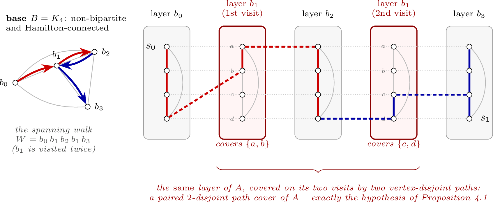
Write a spanning walk as \(W=(w_0,\ldots,w_{N-1})\), where \(N\) is its number of layer occurrences, and write \(\alpha_0,\ldots,\alpha_N\) for the \(A\)-coordinates at the boundaries of the layer pieces. Thus the piece in occurrence \(w_i\) runs from \(\alpha_i\) to \(\alpha_{i+1}\), with \(\alpha_0=a_0\) and \(\alpha_N=a_1\). Every single-layer Hamilton path and both paths in every doubled-layer cover have opposite-colored ends. Hence \[\chi(\alpha_{i+1})=1-\chi(\alpha_i)\quad(0\le i<N),\] and telescoping gives the single requirement \[N\equiv\chi(a_0)\oplus\chi(a_1)\pmod2.\]

The doubled-layer device needs spanning walks of \(B\) of a prescribed parity repeating no vertex more than twice. The next claim supplies them, using only that \(B\) is Hamilton-connected (hence, on \(\ge3\) vertices, \(2\)-connected).

Proof of Claim. The needed neighbors can be read off Hamilton paths directly. If \(s\ne t\): a Hamilton path \(s\to t\) gives \(N=n\); its penultimate vertex \(w\) is a neighbor of \(t\) with \(w\ne s\) (a Hamilton path on \(n\ge3\) vertices visits each vertex once, and \(w\) is not the first), so a Hamilton path \(s\to w\) followed by the edge \(wt\) gives \(N=n+1\) with \(t\) the only repeated vertex. If \(s=t\): the second vertex \(u\) of any Hamilton path out of \(s\) is a neighbor of \(s\), and a Hamilton path \(s\to u\) closed by the edge \(us\) gives \(N=n+1\); taking a neighbor \(m\) of \(s\) and the penultimate vertex \(u'\) of a Hamilton path \(s\to m\) (a neighbor of \(m\) with \(u'\ne s\)), a Hamilton path \(s\to u'\) followed by \(u'\,m\,s\) gives \(N=n+2\), with \(s\) (the required return) and \(m\) the only repeated vertices. \(\square\)

The four Claim constructions have, respectively, zero, one, one, and two doubled layers. In the open \(N=n+1\) walk, the earlier occurrence of \(b_1\) is internal in the fresh Hamilton path, at some position \(1\le j\le n-2\), so its boundary pair is disjoint from the final pair. In the closed \(N=n+1\) walk, the two occurrences of \(b_0\) are first and last and their boundary pairs are disjoint because \(n\ge3\). If \(b_0=b_1\), then \(a_0\ne a_1\), since the two product endpoints are distinct. The remaining two-doubled-layer incidence is analyzed below.

Apply the claim with \((s,t)=(b_0,b_1)\). The two walks have opposite \(N\)-parities, so one satisfies the displayed requirement; take it as \(W\). Its repeated vertices are the doubled layers: at most \(b_1\) when \(b_0\ne b_1\), and at most \(b_0\) together with one other layer when \(b_0=b_1\). Every singly visited layer will receive a Hamilton path of \(A\). We now make the global boundary choice that supplies valid demands in all doubled layers.

Proof. The colors of all boundaries are forced by \(\chi(a_0)\) and their indices. With no doubled layer, choose any vertex of the required color at each free boundary. With one doubled layer, its four terminals contain at most the two distinct pins \(a_0,a_1\). Their forced colors occur twice each. If the two pins have the same color, they already occupy the two terminals of that color and we choose two distinct vertices of the other color. If the pins have opposite colors, choose in each color a second vertex distinct from its pin. The cases with one or no pin are easier. Each color class has at least two vertices, so all choices exist.

It remains to treat the closed walk with \(N=n+2\), where the two doubled layers may have two common boundaries. Use the notation of the Claim. Let \[x_0=b_0,x_1,\ldots,x_{n-1}=u'\] be the fresh Hamilton path from \(b_0\) to \(u'\), and let \(m=x_k\). Since \(m\ne b_0,u'\), we have \(1\le k\le n-2\), and \[W=(x_0,x_1,\ldots,x_{n-1},m,b_0).\] The doubled \(b_0\)-layer has terminal pairs \[(\alpha_0,\alpha_1),\qquad(\alpha_{n+1},\alpha_{n+2}),\] and the doubled \(m\)-layer has \[(\alpha_k,\alpha_{k+1}),\qquad(\alpha_n,\alpha_{n+1}).\] The layers always share \(\alpha_{n+1}\). If \(k=1\), equivalently if the fresh Hamilton path begins \(b_0,m,\ldots\), they also share \(\alpha_1\). This is the two-shared-boundary configuration; for \(B=K_3\) it is forced. When \(k=n-2\), one has \(k+1=n-1<n\), so \(\alpha_{k+1}\) is not the boundary occurrence \(\alpha_n\) and no further shared boundary is created. For \(n=3\), one has \(k=1=n-2\), and the two-shared-boundary configuration just identified is the unique detour shape.

Choose the relevant boundaries in the order used by the formal construction. First choose \(\alpha_{n+1}\) in its forced color, distinct from \(a_0=\alpha_0\). Next choose \(\alpha_1\) in its forced color. The vertices \(a_1=\alpha_{n+2}\) and \(\alpha_{n+1}\) have opposite colors, so exactly one of them has the color of \(\alpha_1\); avoid that one. The four terminals of the \(b_0\)-layer are now distinct. Choose \(\alpha_n\) in its forced color, avoiding \(\alpha_1\) when their colors agree.

If \(k=1\), set \(\alpha_k=\alpha_1\) and choose \(\alpha_{k+1}\) in its forced color, avoiding the one member of \(\{\alpha_n,\alpha_{n+1}\}\) having that color. The four terminals of the \(m\)-layer are then distinct. If \(k>1\), choose \(\alpha_k\) and \(\alpha_{k+1}\) in their forced, opposite colors; each avoids the unique same-colored member of \(\{\alpha_n,\alpha_{n+1}\}\). Choose all remaining boundaries arbitrarily in their forced colors.

This order also proves the extremal case in which each color class of \(A\) has exactly two vertices. At every choice, at most one previously chosen vertex of the required color is excluded; vertices of the opposite color are automatically distinct. Hence a choice remains in a two-element color class. Both the one- and two-shared-boundary configurations are covered. \(\square\)

With the boundaries fixed, each singly-visited layer is traversed by a Hamilton path of \(A\) between its opposite-colored boundaries (Hamilton-laceability), and each doubled layer — including the layer carrying both pins \(a_0\ne a_1\) in the same-\(B\)-layer case — by a paired \(2\)-cover, whose four terminals are distinct and balanced by Lemma 4.2, so the paired-cover hypothesis on \(A\) supplies it. Splicing all the layer pieces across the matching along \(W\) yields the Hamilton \(s_0\)–\(s_1\) path. \(\square\)

Remark. The Lean theorem boxProd_hamConnected_paper implements the walk argument above. Its walk_pass_cycle_detour branch uses the same order of boundary choices; when \(k=1\), it explicitly reuses \(\alpha_1\) as the first terminal of the doubled \(m\)-layer. The helper lemmas walk_pick_color_ne and walk_pick_terminals formalize the one-exclusion choices, including two-element color classes. An independent absorber construction of the same covers is retained as an alternate proof.

The degenerate factor \(A=K_2\). When \(|V(A)|=2\) the doubled-layer device is unavailable (a paired \(2\)-cover needs four distinct terminals), and \(G=K_2\,\square\,B\) is the prism over \(B\): two copies \(B^0,B^1\) joined by the rungs \(v^0v^1\). We prove it Hamilton-connected directly, using only that \(B\) (Hamilton-connected by the induction hypothesis, with \(n=|V(B)|\ge3\)) has a Hamilton path between any two distinct vertices. Let the endpoints be \((i,u)\) and \((j,w)\).

• Different copies (\(i\ne j\), say \((0,u)\to(1,w)\)): pick \(x\notin\{u,w\}\) (possible as \(n\ge3\); if \(u=w\) any \(x\ne u\)). A Hamilton path \(u\to x\) of \(B^0\), the rung \(x^0x^1\), and a Hamilton path \(x\to w\) of \(B^1\) concatenate into a Hamilton path of the prism.

• Same copy (\(i=j\), say \((0,u)\to(0,w)\) with \(u\ne w\)): take a Hamilton path \(u=h_0,h_1,\dots,h_{n-1}=w\) of \(B\). Then \[\begin{align}&(0,h_0)\to(1,h_0)\to[\,\text{a fresh Hamilton path }h_0\to h_1\text{ of }B^1\,]\\&\qquad\to(1,h_1)\to(0,h_1)\to(0,h_2)\to\cdots\to(0,h_{n-1})\end{align}\] is a Hamilton path of the prism: \(B^1\) is covered by the interior Hamilton path \(h_0\to h_1\), and \(B^0\) by \((0,h_0)\) together with the tail \((0,h_1),\dots,(0,h_{n-1})\).

Hence every pair of prism vertices is joined by a Hamilton path, so \(K_2\,\square\,B\) is Hamilton-connected. \(\square\)

This section handles case (iii), the largest branch and the only genuinely new construction: the indecomposable non-bipartite prime classes. It applies the induction hypothesis to the fibers of a separating line and uses the Naddef–Pulleyblank dichotomy to obtain Hamilton-connectedness of the non-bipartite matroid base-exchange quotient.

Let \(G=G(R,S)\) be a nonempty class normalized by deleting inactive lines, and assume that it is invariant-free (hence prime/indecomposable by §2.2), non-bipartite, has \(m,n\ge3\) active rows and columns, and has \(|V(G)|>6\). Fix distinct vertices \(a,b\in V(G)\). For a line \(L\), write \(F_p\) for the fiber obtained by fixing \(L\) to the realizable pattern \(p\), and write \(Q_L\) for the line quotient. Three notions recur:

• a line \(L\) is separating (for \(a,b\)) if \(a\) and \(b\) have different patterns on \(L\);

• the buffer line is the separating line produced by Lemma 5.9, one of whose fibers — the buffer — is non-bipartite; it is the line we build the final path around, and its row is the pivot row;

• a quotient edge is used if the lifted path crosses it.

Every lemma in this section is stated within this regime (active, invariant-free, indecomposable, non-bipartite, \(m,n\ge3\)). The order bound \(|V(G)|>6\) selects the §5 branch rather than the §6 branch; it is not used in the local proofs of Lemmas 5.8–5.10.

The whole construction is four steps, each licensed by the lemma named beside it; the reader may hold this skeleton while the lemmas supply the guarantees; it is restated as an explicit algorithm and run on a worked example at the end of the section. Given distinct endpoints \(a,b\): (1) choose a separating buffer line \(L\) with a non-bipartite fiber (Lemma 5.9); (2) its quotient \(Q_L\) is a non-bipartite matroid base-exchange graph, hence Hamilton-connected (Lemmas 5.3, 5.4, 5.10, Corollary 5.5); (3) take a Hamilton path of \(Q_L\) from the fiber of \(a\) to the fiber of \(b\); (4) thread the fibers along that path, traversing each by a recursively obtained Hamilton path and splicing consecutive fibers on interface edges (Lemmas 5.6, 5.7, Proposition 5.11). The buffer fiber absorbs the parity that a chain of forced fibers could not.

Figure 2 shows the whole construction on a small class, and the reader may find it useful to hold while the lemmas arrive; it is the class worked in full at the end of the section.

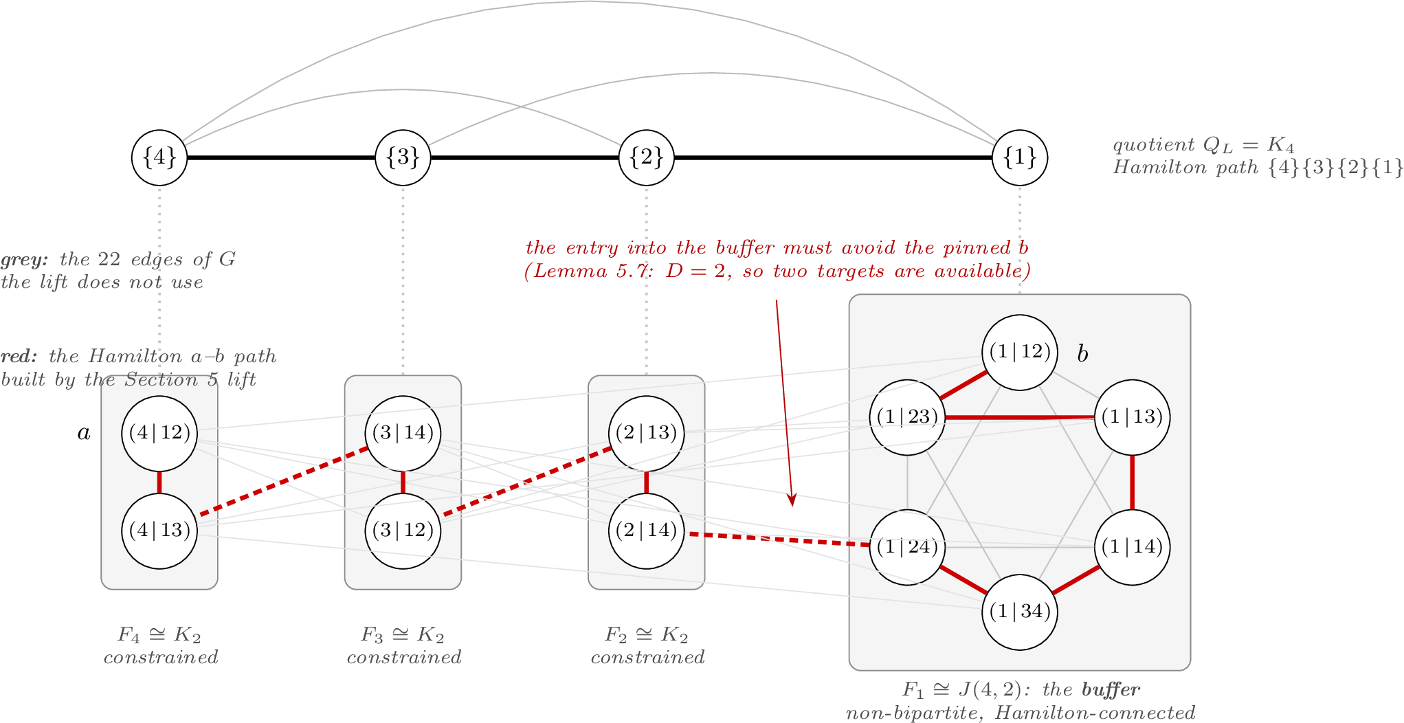
Throughout this section every fiber is immediately put into canonical normal form: delete inactive lines, then split the invariant positions into their Cartesian factors (§2.2). The induction hypothesis applies to any strictly smaller interchange graph — in particular to the resulting invariant-free factors, and to whole fiber cores where convenient. In particular, the induction hypothesis includes every fiber of order at most six and every Johnson fiber. The smaller instance follows the ordinary §3 dispatch: a bipartite fiber is handled outright by Lemma 1.2, a decomposable non-bipartite fiber by §4, a Johnson fiber by the §6 Johnson branch, and a remaining prime many-line fiber of order at most six by the §6 finite branch. Thus an order-six fiber inside a larger §5 class is already covered by the strong induction, not a new §5 case.

Proof. Fixing \(L\) to \(p\) gives a proper subclass, since \(L\) is separating and hence at least two line patterns occur in \(G\). Deleting \(L\) leaves a complete-margin \(0\)-\(1\) matrix class on fewer lines. Any inactive line in this class is forced in every matrix of the fiber, so deleting it is graph-isomorphic. Any remaining invariant position gives the Cartesian factorization of §2.2: the variable cells split into diagonal blocks and the off-block rectangles are forced. Thus the fiber graph is a Cartesian product of the interchange graphs of those variable blocks.

Each block is strictly smaller than \(G\): the fiber has fewer vertices than \(G\), and every nontrivial factor has at most the fiber order. \(\square\)

Proof. The block is prime (§2.2), so this is the theorem of Brualdi and Manber [11]: an active prime class has no invariant cell — every row-column position varies in some realization. \(\square\)

Remark. One can also derive this from the theory of forced entries (Brualdi [3]): a forced cell is exactly a cell separated from the variable part by a tight row-column cut; in an active class all inactive-line forced cells have been deleted, and in an invariant-free block no nontrivial forced off-diagonal rectangle remains — otherwise the block would split as a nontrivial Cartesian product.

Let \(L\) be a row; the column case is obtained by transposition. Let \(k=r_L\), let \(R'\) be the row-sum vector after deleting \(L\), and let \(S=(s_1,\ldots,s_n)\). A pattern \(p\subseteq[n]\), \(|p|=k\), is realizable exactly when the residual column vector \(S-\mathbf{1}_p\) is realizable with row sums \(R'\).

For \(X\subseteq[n]\) put \[h(X)=\sum_i \min(r'_i,|X|),\qquad \ell(X)=\sum_{j\in X}s_j-h(X).\] By the Gale–Ryser theorem [1], [13] (see also Brualdi [3]), \(p\) is realizable if and only if \[|p|=k,\qquad |p\cap X|\ge \ell(X)\quad\text{for every }X\subseteq[n].\] The function \(h(X)\) depends only on \(|X|\) and is submodular, since \(q\mapsto\sum_i\min(r'_i,q)\) is discrete concave. Hence \(\ell\) is supermodular. (Two ambient facts absorbed into the display: \(\sum_j s_j=k+\sum_i r'_i\), since the class is nonempty; and every column is active in the §5 regime, so the residual entries are nonnegative wherever it matters.)

Proof. Let \(\mathcal{B}\) be the family of \(k\)-subsets satisfying the Gale–Ryser inequalities above. We verify the basis-exchange axiom. Let \(A,B\in\mathcal{B}\) and \(e\in A\setminus B\). Put \(A_0=A\setminus\{e\}\). A set \(X\) is deficient for \(A_0\) if \(|A_0\cap X|<\ell(X)\). Such an \(X\) must contain \(e\), and since \(A\) was feasible, necessarily \(|A_0\cap X|=\ell(X)-1\).

Deficient sets are closed under intersection. If \(X,Y\) are deficient, then using modularity of cardinality and supermodularity of \(\ell\), \[\begin{align} |A_0\cap(X\cap Y)| &=|A_0\cap X|+|A_0\cap Y|-|A_0\cap(X\cup Y)|\\ &\le \ell(X)+\ell(Y)-2-(\ell(X\cup Y)-1) \le \ell(X\cap Y)-1 \end{align}\] (the middle step also uses \(|A_0\cap(X\cup Y)|\ge\ell(X\cup Y)-1\), which holds for every set by \(A\)’s feasibility less one element). The family of deficient sets is nonempty: the ground set \([n]\) is itself deficient, since \(h([n])=\sum_i r'_i\) gives \(\ell([n])=k\) while \(|A_0\cap[n]|=|A_0|=k-1\). Thus the intersection \(Z\) of all deficient sets (a finite, intersection-closed, nonempty family) is deficient. Since \(B\) is feasible, \[|B\cap Z|\ge \ell(Z)=|A_0\cap Z|+1.\] As \(e\notin B\), this gives an element \(f\in B\setminus A\) with \(f\in Z\). Then \(A-e+f\) meets every deficient set, and all non-deficient inequalities were already satisfied by \(A_0\). Hence \(A-e+f\in\mathcal{B}\). \(\square\)

Remark. The matroid property of single-line patterns is classical in spirit — by Gale–Ryser the realizable patterns are the integer points of a polymatroid slice, and such families form matroid bases (Edmonds [14]) — and we keep the short self-contained proof above. The Lean companion contains two machine-checked proofs of Lemma 5.3. Its main proof follows the deficient-set argument above as printed, on top of a self-contained mechanization of the Gale–Ryser existence theorem. An independent alternate is also included: among realizations \(M\in F_A\), \(N\in F_B\) choose a pair minimizing the number of differing cells; two local interchange arguments then force a closure property on the difference pattern, and a counting identity over the difference cells produces the exchange as a single explicit interchange. The proofs are independent, so the lemma is doubly verified. (The same minimal-pair technique proves the unit-transfer Lemma 5.4 below, whose proof we give in that form.)

Proof. Write \(c=S-\mathbf{1}_p\) for the residual column-sum vector of the non-pivot rows when \(L=p\), and \(c'=S-\mathbf{1}_q=c+e_i-e_j\); the residual classes \(\mathcal{A}'=\mathcal{A}(R',c)\) and \(\mathcal{B}'=\mathcal{A}(R',c')\) are both nonempty, by the realizability of \(p\) and of \(q\). Suppose, for contradiction, that no matrix of \(\mathcal{A}'\) has a row of type \((0,1)\) in columns \((i,j)\): then in every member of \(\mathcal{A}'\), every row with a \(1\) in column \(j\) also has a \(1\) in column \(i\).

Choose a pair \((M,N)\in\mathcal{A}'\times\mathcal{B}'\) minimizing the number of cells at which \(M\) and \(N\) differ. Call a cell a P-cell if \(M\) has a \(1\) and \(N\) a \(0\) there, and a Q-cell in the opposite case. In each column \(k\), the count of P-cells minus Q-cells equals \(c_k-c'_k\): zero for \(k\ne i,j\), \(+1\) for \(k=j\) (and \(-1\) for \(k=i\), which we shall not need). Hence the row set \[\mathcal{S}=\{a:\;(a,j)\text{ is a P-cell}\}\] is nonempty, and every \(a\in\mathcal{S}\) has \(M_{aj}=1\), so also \(M_{ai}=1\) by our assumption. Let \(\mathcal{T}\) be the set of columns containing a Q-cell of some row of \(\mathcal{S}\). Then \(j\notin\mathcal{T}\) and \(i\notin\mathcal{T}\) (rows of \(\mathcal{S}\) carry \(1\)s of \(M\) in both columns).

Closure: for \(k\in\mathcal{T}\), every P-cell of column \(k\) lies in a row of \(\mathcal{S}\). Let \((b,k)\) be a P-cell and pick \(a\in\mathcal{S}\) with a Q-cell at \((a,k)\); then \(a\ne b\) and \(k\ne j\) (row \(a\) has \(M_{aj}=1\) but \(M_{ak}=0\)). The known cells so far: \[\begin{array}{c|ccc} & (a,j) & (a,k) & (b,k)\\\hline M & 1 & 0 & 1\\ N & 0 & 1 & 0 \end{array}\] If \(M_{bj}=0\), the block on rows \(\{a,b\}\) and columns \(\{j,k\}\) of \(M\) is switchable (\(M_{aj}=M_{bk}=1\), \(M_{ak}=M_{bj}=0\)); the switch stays in \(\mathcal{A}'\) and flips four cells of which at least three, namely \((a,j)\), \((a,k)\), \((b,k)\), were differences from \(N\), so it strictly decreases the difference count, contradicting minimality. Hence \(M_{bj}=1\).

If \(N_{bj}=1\), the block on rows \(\{b,a\}\) and columns \(\{j,k\}\) of \(N\) is switchable (\(N_{bj}=N_{ak}=1\), \(N_{bk}=N_{aj}=0\)); the switch stays in \(\mathcal{B}'\) and again flips at least three current differences, namely \((b,k)\), \((a,j)\), \((a,k)\), contradicting minimality. Hence \(M_{bj}=1\) and \(N_{bj}=0\), i.e. \(b\in\mathcal{S}\).

Counting. Fix \(a\in\mathcal{S}\). Rows of \(M\) and \(N\) have equal sums, so row \(a\) has exactly as many P-cells as Q-cells. All its Q-cells lie in \(\mathcal{T}\)-columns (by the definition of \(\mathcal{T}\)), while among its P-cells the cell \((a,j)\) lies outside \(\mathcal{T}\); hence its P-cells in \(\mathcal{T}\)-columns number at most its Q-cells in \(\mathcal{T}\)-columns minus one. Summing over \(\mathcal{S}\) and recounting by columns, \[\sum_{k\in\mathcal{T}}P^{\mathcal{S}}_k+|\mathcal{S}|\;\le\;\sum_{k\in\mathcal{T}}Q^{\mathcal{S}}_k,\] where \(P^{\mathcal{S}}_k,Q^{\mathcal{S}}_k\) count the P- and Q-cells of column \(k\) in rows of \(\mathcal{S}\). But each \(k\in\mathcal{T}\) has \(k\ne i,j\), so column \(k\) has equally many P- and Q-cells in total; the closure property gives \(P^{\mathcal{S}}_k=P_k\), and trivially \(Q^{\mathcal{S}}_k\le Q_k=P_k\). Hence the right side is at most the left sum without the \(|\mathcal{S}|\) term, forcing \(|\mathcal{S}|\le 0\) — contradicting \(\mathcal{S}\ne\emptyset\).

Therefore some matrix of \(F_p\) has a non-pivot row of type \((0,1)\) in columns \((i,j)\); switching that row against \(L\) on columns \(\{i,j\}\) realizes the exchange \(p\to q\) as an actual crossing edge between \(F_p\) and \(F_q\). \(\square\)

Remark. The argument above is the one verified in the Lean companion. Alternatively, the lemma follows from Gale–Ryser tightness (Brualdi [3]): column \(j\) is contained in column \(i\) in every member of a nonempty class exactly when some column set \(X\) with \(i\in X\), \(j\notin X\) is Gale–Ryser-tight, equivalently when the transferred margin vector \(c+e_i-e_j\) is infeasible — a criterion derived there from the Gale–Ryser theorem; applying it with the residual margins of \(p\) gives the row sought.

By Lemma 5.4 every basis exchange of \(M_L\) is realized by a crossing edge, and conversely every crossing interchange changes the line pattern by exactly one basis exchange. Therefore \(Q_L\) equals the basis-exchange graph of \(M_L\), i.e. the \(1\)-skeleton of the matroid base polytope \(\operatorname{conv}\{\mathbf{1}_B:B\in\mathcal{B}(M_L)\}\) (two bases are polytope-adjacent exactly when they differ by a single exchange — a criterion of Edmonds, first in print in Hausmann–Korte [15]; see also [16]).

Proof. By Lemmas 5.3–5.4, \(Q_L\) is the \(1\)-skeleton of a matroid base polytope. By Naddef–Pulleyblank [16] Theorem 3.3.1 and Corollary 3.3.2, the graph of a matroid base polytope is either a hypercube or Hamilton-connected. Since \(Q_L\) is non-bipartite, the hypercube alternative is impossible. \(\square\)

Call a fiber constrained if its canonical core is bipartite of order at least \(2\). By the bipartite classification it is balanced, and by the induction hypothesis it is Hamilton-laceable. Call a fiber free if it is non-bipartite or a singleton. A non-bipartite free fiber is Hamilton-connected by induction; a singleton imposes no internal parity condition. In summary:

constrained	Hamilton-laceable; exit color forced	whole fiber (5.6); two reachable targets (5.7)
non-bipartite	Hamilton-connected (induction)	\(\ge2\) interface vertices (5.6); two-sided avoid (5.7)
singleton	trivial	no parity constraint; freedom supplied on the far side (5.6)

(In the worked example closing the section, the buffer fiber is the octahedron \(J(4,2)\) and the three other fibers are single edges \(K_2\) — the reader may find it useful to glance at that instance while reading Lemmas 5.6–5.7.) These two lemmas are consumed only in the gluing of Proposition 5.11; a reader may take their statements on a first pass and return to the proofs alongside the gluing.

Proof. A crossing switch \(p\to q\) at \(M\in F_p\) exists exactly when some non-pivot row of \(M\) has type \((0,1)\) in columns \((i,j)\); so the non-interface is the nesting locus \[N=\{M\in F_p:\operatorname{supp}_j(M)\subseteq \operatorname{supp}_i(M)\},\qquad I_{p\to q}=V(F_p)\setminus N.\] Suppose \(N\) is neither empty nor all of \(F_p\). Since fibers are connected, there is an internal edge \(M M'\) with \(M\in N\) and \(M'\notin N\). The switch \(M\to M'\) uses exactly one of the columns \(i,j\): using neither would leave the nesting unchanged, and using both would exhibit a \((0,1)\)-row already in \(M\). Say it uses columns \(i,c\); then \(M\) has two rows \[u:(i,j,c)=(1,1,0),\qquad v:(i,j,c)=(0,0,1),\] and the alternate switch on columns \(j,c\) produces a third vertex \(M''\notin N\) with \(M''\ne M'\). (Columns \(j,c\) is symmetric.)

If \(F_p\) is bipartite, then \(M,M',M''\) differ pairwise by single switches — \(M'\) from \(M\) on \(\{i,c\}\), \(M''\) from \(M\) on \(\{j,c\}\), and \(M'\) from \(M''\) on \(\{i,j\}\) — a triangle, contradicting bipartiteness. Hence \(N\) is empty or all of \(F_p\). Since \(p,q\) are adjacent, Lemma 5.4 realizes the quotient edge, so \(I_{p\to q}\ne\emptyset\) and \(N\ne F_p\); thus \(N=\emptyset\) and \(I_{p\to q}=V(F_p)\).

If \(F_p\) is non-bipartite and the edge is used, then \(I_{p\to q}\ne\emptyset\), so \(N\ne F_p\). If \(N=\emptyset\) then \(I_{p\to q}=V(F_p)\), which has at least three vertices since \(F_p\) contains a triangle. Otherwise the boundary edge above gives two distinct interface vertices \(M',M''\). Either way \(|I_{p\to q}|\ge 2\). \(\square\)

Thus on a used edge whose source is constrained (bipartite), the source-side interface is the whole fiber — both exit colors are available and there is no exit pin — and on a used edge at any non-bipartite fiber at least two interface vertices are available. The gluing needs slightly more than this bare count when a constrained fiber exits at a forced color, so we must know that color reaches sufficiently many vertices of the adjacent non-bipartite fiber.

Proof. For \(X\in C\) let \(a(X),b(X),t(X)\) count the non-\(L\) rows of type \((1,0),(0,1),(1,1)\) in columns \((i,j)\). Row \(L\) of \(X\) has type \((1,0)\), contributing \(1\) to column \(i\) and \(0\) to column \(j\), so counting the \(1\)’s in columns \(i,j\) over all rows gives \(1+a(X)+t(X)=s_i\) and \(b(X)+t(X)=s_j\), whence \[b(X)-a(X)=D:=s_j-s_i+1\qquad(X\in C).\] Each type-\((0,1)\) row of \(X\) yields one crossing from \(X\) into \(E\) (switch it against row \(L\) on columns \(\{i,j\}\)), distinct rows giving distinct neighbors, so \(b(X)\) is the number of crossings from \(X\) into \(E\). Symmetrically each \(Y\in E\) (whose row \(L\) has type \((0,1)\)) satisfies \(r(Y)-r'(Y)=s_i-s_j+1=2-D\), where \(r(Y),r'(Y)\) count its \((1,0)\)- and \((0,1)\)-rows and \(r(Y)\) is the number of crossings from \(Y\) back to \(C\).

(i) \(C\) constrained. Two values of \(D\) are excluded. If \(D=1\) then \(s_i=s_j\), so transposing columns \(i,j\) is an automorphism of \(G(R,S)\) carrying \(p\) to \(q\) and hence \(C\) isomorphically onto \(E\) — impossible, since \(C\) is bipartite and \(E\) is not. If \(D<0\) then \(2-D\ge 3\), so every \(Y\in E\) has \(r(Y)\ge 3\); switching \(L\) against three of \(Y\)’s \((1,0)\)-rows produces three vertices of \(C\) pairwise joined by interchanges on columns \((i,j)\) — a triangle in the bipartite \(C\), again impossible. Hence \(D=0\) or \(D\ge 2\). If \(D\ge 2\), then \((\ast)\) gives \(b(X)\ge 2\) for every \(X\in C\). If \(D=0\), every \(Y\in E\) has \(r(Y)\ge 2\), and \(C\) (constrained, hence balanced bipartite) has \(|V(C)|\) even: when \(|V(C)|=2\), switching \(L\) against two \((1,0)\)-rows of any \(Y\in E\) gives the two vertices of \(C\), so each vertex of \(C\) is adjacent to all of \(E\) (and \(|V(E)|\ge 3\), as \(E\) contains a triangle); when \(|V(C)|\ge 4\), a color class \(\kappa\) reaching a single \(e\in E\) would have every \(M\in\kappa\) (whole-fiber interface, Lemma 5.6) cross only to \(e\), so each such \(M\) is \(e\) with its unique crossing switch undone on rows \(\{L,r_M\}\) and columns \(\{i,j\}\), whence any two differ by one interchange and \(\kappa\) is a clique in the bipartite \(C\) — impossible. In every case each color class reaches at least two vertices of \(E\), so the forced exit color reaches one \(\ne\mathit{bad}\).

(ii) \(C\) non-bipartite. Put \(c_C:=D\) and \(c_E:=2-D\), so \(c_C+c_E=2\); the sought conclusion is symmetric under \((C,x)\leftrightarrow(E,\mathit{bad})\) (which swaps \(c_C\leftrightarrow c_E\)), so we may assume \(c_C\ge 1\). Both fibers contain a triangle, so \(|C|,|E|\ge 3\). If \(c_C\ge 2\), then \((\ast)\) gives \(b(X)\ge 2\) for every \(X\in C\); choose \(X\ne x\) (possible as \(|C|\ge 3\)), so \(X\) has two crossings to distinct vertices of \(E\), at most one being \(\mathit{bad}\), and we take \(y:=X\), \(z\ne\mathit{bad}\). If \(c_C=1\) (so \(c_E=1\) and \(s_i=s_j\)), suppose every crossing is incident to \(x\) or \(\mathit{bad}\). Pick distinct \(X_1,X_2\in C\setminus\{x\}\); each has a crossing (as \(b(X_t)=a(X_t)+1\ge 1\)), not to \(x\), hence to \(\mathit{bad}\), so \(r(\mathit{bad})\ge 2\). The crossing \(\mathit{bad}\,X_1\) switches rows \(\{L,a\}\) for a \((1,0)\)-row \(a\) of \(\mathit{bad}\), so the type-\((0,1)\) rows of \(X_1\) are those of \(\mathit{bad}\) together with \(a\), giving \(b(X_1)=r'(\mathit{bad})+1=r(\mathit{bad})\ge 2\) (using \(r(\mathit{bad})-r'(\mathit{bad})=2-D=1\)). But then every crossing of \(X_1\) runs to \(\mathit{bad}\), so \(b(X_1)\le 1\) — a contradiction. In either subcase a crossing \(yz\) has \(y\ne x\) and \(z\ne\mathit{bad}\); a Hamilton path of \(C\) from \(x\) to \(y\) (Hamilton-connectedness, induction hypothesis) then delivers \(z\ne\mathit{bad}\) into \(E\). \(\square\)

(The Lean companion’s main proof is the argument above as printed; the avoid form the gluing consumes also carries an independent constructive proof, handling all \(D\le 1\) without the two exclusion steps.)

Clause (i) lets a constrained fiber, whose exit color is forced, still hand the non-bipartite target an entry distinct from its pinned exit; clause (ii) is the symmetric non-bipartite-source case. A singleton source is a deterministic pass-through: its used edge is already realized, and the two interface vertices of Lemma 5.6 on the non-bipartite side supply an entry \(\ne\mathit{bad}\).

Call a pair of rows a wide pair if, in some realization of \(G(R,S)\), their supports are incomparable (each has a \(1\) in some column where the other has a \(0\)) and their symmetric difference has size at least \(3\); wide column pairs are defined dually. Triangles are governed by these.

Proof. Let \(M_0,M_1,M_2\) be a triangle. Each symmetric difference \(M_i\triangle M_j\) is the support of a single interchange: four cells \(\{a,b\}\times\{i,j\}\) carrying the \(2\times2\) checkerboard pattern. From \(M_0\triangle M_2=(M_0\triangle M_1)\triangle(M_1\triangle M_2)\), the symmetric difference of the two interchange-supports \(S_1=M_0\triangle M_1\) and \(S_2=M_1\triangle M_2\) is itself a single interchange-support, so \(|S_1\triangle S_2|=4\) and hence \(|S_1\cap S_2|=2\). Writing \(S_1=\{a,b\}\times\{i,j\}\), the two shared cells lie in \((\{a,b\}\cap\mathrm{rows}(S_2))\times(\{i,j\}\cap\mathrm{cols}(S_2))\); two cells force either both rows shared with a single column, or a single row shared with both columns (a shared diagonal would force \(S_2=S_1\)). The exact complementary cardinality follows directly. In the first case the two supports use the same two rows, and their two-column sets intersect in one column; since \(S_1\ne S_2\), their union therefore has \(2+2-1=3\) columns. In the second case their two-row sets intersect in one row and their column sets agree, so their union has \(2+2-1=3\) rows and exactly two columns. The remaining support \(M_0\triangle M_2\) lies in the same two rows (resp. columns), so the whole triangle is supported on two rows and three columns, or on three rows and two columns. Its two rows (resp. columns) carry the three rotations of the \(2\times3\) (resp. \(3\times2\)) pattern, so they differ in all three changing columns (rows) — a wide pair. \(\square\)

Since a non-bipartite interchange graph contains a triangle (Lemma 2.1, equivalently Brualdi [3] Thm. 6.3.4), it has a wide row pair or a wide column pair.

Proof. A triangle in \(G\) lies in an \(L\)-fiber exactly when it does not use the line \(L\). Hence a separating line \(L\) has a non-bipartite fiber if and only if some triangle avoids \(L\).

Suppose no separating line has a non-bipartite fiber. Then every triangle uses every separating row and every separating column of the pair \(a,b\). Let \(R^*\) and \(C^*\) be the separating rows and columns. Since \(a\) and \(b\) have the same margins, their difference is a union of alternating cycles, so \(|R^*|,|C^*|\ge2\).

Every triangle in an interchange graph is either a two-row triangle using exactly two rows and three columns, or a three-row triangle using exactly three rows and two columns (Lemma 5.8). Therefore, if \(|R^*|\ge4\) or \(|C^*|\ge4\), no triangle can meet all separating lines, contradiction. If \(|R^*|=|C^*|=3\), a two-row triangle misses a separating row and a three-row triangle misses a separating column, again a contradiction. In summary:

\[\begin{array}{ll} |R^*|\ge4\text{ or }|C^*|\ge4 & \text{impossible: every triangle misses a separating line}\\ (3,3) & \text{impossible: each triangle type misses one side}\\ (2,2),\;(2,3),\;(3,2) & \text{the remaining cases, handled below} \end{array}\]

We also use the converse of the triangle classification: a wide row pair \(\{p,q\}\) supports a triangle on those two rows. Their symmetric difference \(\Delta\) has \(|\Delta|\ge3\) with both sides nonempty, so one side—say \(p\)’s—has at least two columns; taking two columns from \(p\)’s side and one from \(q\)’s gives a \(2\times3\) block whose three rotations are interchanges (each preserves all margins), hence lie in \(G\) and form a triangle on rows \(\{p,q\}\) (dually for columns).

In the remaining cases, every wide row pair must be the unique two-row set \(R^*\) when \(|R^*|=2\), and no wide row pair can exist when \(|R^*|=3\). Similarly, every wide column pair must be the unique two-column set \(C^*\) when \(|C^*|=2\), and no wide column pair can exist when \(|C^*|=3\). Thus \(G\) has at most one wide row pair and at most one wide column pair.

Claim: a unique wide row pair (or column pair) cannot exist. Suppose \(\{p,q\}\) is the unique wide row pair, and let \(V\) be the unique wide column pair if one exists, and \(V=\emptyset\) otherwise. Choose a realization \(M\) in which \(p,q\) are wide, and write \[A=R_p(M)\setminus R_q(M),\quad B=R_q(M)\setminus R_p(M),\quad \Delta=A\cup B,\] with \(A,B\ne\emptyset\) and \(|\Delta|\ge3\). Choose \(d\in \Delta\) not belonging to \(V\), possible because \(V\) has at most two columns.

Along any interchange path from \(M\), track the current supports of rows \(p,q\) through the split \[A_t=R_p\setminus R_q,\qquad B_t=R_q\setminus R_p,\qquad (A_0,B_0)=(A,B),\] where \(R_p,R_q\) denote the supports in the current realization, and consider the invariant “rows \(p,q\) are wide with the same difference set \(\Delta=A_t\cup B_t\)”: the split \((A_t,B_t)\) may change from step to step, but \(\Delta\) and the side sizes \(|A_t|,|B_t|\) do not. Take the first switch (if any) that uses exactly one row from \(\{p,q\}\) and one outside row — say rows \(p\) and \(x\notin\{p,q\}\), on columns \(u,v\). Just before it the invariant still holds. The switch’s checkerboard puts \(u\in\operatorname{supp}(p)\setminus\operatorname{supp}(x)\) and \(v\in\operatorname{supp}(x)\setminus\operatorname{supp}(p)\), so \(p,x\) are incomparable in the current realization; since \(\{p,x\}\) is not wide, their symmetric difference is exactly \(\{u,v\}\), so after the switch \(R_x\) equals row \(p\)’s pre-switch support: \(\{x,q\}\) inherits the pre-switch split \((A_t,B_t)\) of \(\Delta\) and is wide in the post-switch realization — a second wide row pair, contradiction. Thus along any path, \(p,q\) can only switch with each other; such a switch exchanges one column of \(A\) with one of \(B\), so \(|A|\) and \(|B|\) are each preserved and the difference set \(\Delta=A\cup B\) remains fixed — the invariant persists.

Pick a third row \(x\notin\{p,q\}\). By Lemma 5.2, the cell \((x,d)\) varies; choose a matrix in which its value differs from that in \(M\). By Ryser connectivity (§1), join \(M\) to that matrix by an interchange path and take the first switch on the path that changes \(x_d\). By the previous paragraph this switch uses only rows outside \(\{p,q\}\). Just before the switch, choose \(c\in \Delta\) on the opposite side of the current \(p/q\) split from \(d\). Then columns \(c,d\) differ on rows \(p,q\) with opposite orientations. Since \(d\notin V\), the column pair \(\{c,d\}\) is not wide. Therefore every outside row \(z\) has \(z_c=z_d\); otherwise columns \(c,d\) would differ on \(p,q,z\), forming a wide column pair. In particular \(x_c=x_d\), so the first switch changing \(x_d\) cannot use column \(c\). After the switch, \(x_c\ne x_d\), so columns \(c,d\) now differ on \(p,q,x\), a contradiction.

Thus no such unique wide row pair exists; by transposition no unique wide column pair exists. Since \(G\) is non-bipartite, Lemma 5.8 and its converse give at least one wide row or column pair. Contradiction. Hence some separating line has a non-bipartite fiber. \(\square\)

Proof. Let \(L\) be a row; the column case follows by transposition. The realizable patterns of \(L\) form a shifted matroid \(M_L\): order the columns so \(s_1\ge s_2\ge\cdots\); writing \(S(X)=\sum_{j\in X}s_j\) and \(p(X)=|p\cap X|\), if \(b\in p\), \(a\notin p\) and \(s_a\ge s_b\), then for every \(X\) with \(b\in X,\,a\notin X\) the set \(X'=X-b+a\) satisfies \(S(X')\ge S(X)\) — hence \(\ell(X')\ge\ell(X)\), since \(h\) depends only on the cardinality — and \(p'(X)=p(X')\), so \(p'=p-b+a\) still meets the Gale–Ryser inequalities and is realizable. (For a set \(X\) with \(a\in X\) or \(b\notin X\), the shift leaves \(|p\cap X|\) unchanged or larger, so that inequality is preserved automatically; only \(a\notin X,\,b\in X\) needs the argument just given.) In an active invariant-free block every cell of \(L\) is active (Lemma 5.2), so \(M_L\) is loopless and coloopless on its \(f\ge3\) active columns (\(f=n\) for a row line, \(f=m\) for a column line; \(f\ge3\) by the regime), of some rank \(k\) with \(1\le k\le f-1\).

We use the following elementary consequence of shiftedness. If a basis is required to contain a fixed element \(e\), or required to avoid \(e\), then repeated downward shifts that preserve that requirement carry it to the lexicographically first \(k\)-set satisfying the same requirement, and every intermediate set is a basis. Indeed, let \(T\) be that first \(k\)-set. If a current basis \(B\ne T\) satisfies the requirement, choose the least \(a\in T\setminus B\). Some \(b\in B\setminus T\) has \(b>a\): otherwise every element of \(B\setminus T\) would precede \(a\), making the least element of \(B\triangle T\) lie in \(B\), so that \(B\) itself would be lexicographically earlier than \(T\) — contradicting \(T\)’s choice as the lexicographically first \(k\)-set satisfying the requirement. Replacing \(b\) by \(a\) is a permitted downward shift and preserves the requirement. Iteration terminates at \(T\).

If \(k=1\), looplessness gives the singleton bases \(\{1\},\{2\},\{3\}\), which form a triangle in the base graph. Assume \(k\ge2\). With no constraint, compression gives \(B_0=\{1,\dots,k\}\). Since \(k+1\) is not a loop, some basis contains \(k+1\); compressing among bases containing \(k+1\) gives \(B_1=\{1,\dots,k-1,k+1\}\). Since \(k-1\) is not a coloop, some basis omits \(k-1\); compressing among bases omitting \(k-1\) gives \(B_2=\{1,\dots,k-2,k,k+1\}\). The three bases \(B_0,B_1,B_2\) are pairwise related by a single exchange, so the base graph contains a triangle. By Lemma 5.4, \(Q_L\) is the base graph, so it contains this triangle and is non-bipartite. (The Boolean square \(U_{1,2}\oplus U_{1,2}\), whose base graph is the bipartite \(4\)-cycle, is not shifted, so it never arises as an \(M_L\).) \(\square\)

(The Lean companion’s main proof follows the printed argument throughout — including the shiftedness of \(M_L\), proved by the Gale–Ryser exchange above. Two independent alternates are also machine-checked: a compression by rank-sum minimization, and a shiftedness proof by residual unit transfer.)

Proof. Let \(\alpha,\beta\) be the quotient vertices holding \(a,b\), and choose a Hamilton path \(\alpha=q_0,\ldots,q_t=\beta\) of \(Q_L\) (Hamilton-connected). Since \(Q_L\) is non-bipartite this path has at least three vertices, so each endpoint fiber has a nonempty flanking chain. The non-bipartite fiber \(F=F_{q_s}\) of hypothesis (2) lies on the path. We traverse each fiber by one internal path and splice consecutive fibers on crossing edges.

Fiber traversals. A constrained fiber, once its entry is fixed, exits in the forced opposite color; its whole-fiber interface (Lemma 5.6) realizes an outgoing crossing from any exit vertex of that color, so the next entry may be pinned but this is no obstruction — that fiber simply exits opposite. A singleton is a deterministic pass-through. A non-bipartite fiber other than \(F\) is traversed one-directionally: its entry is delivered from upstream and its exit is chosen on the interface toward the next fiber, which offers at least two vertices (Lemma 5.6), one distinct from the entry; Hamilton-connectedness (induction hypothesis) joins them.

The buffer. Remove \(F\) from the quotient path; the remaining vertices form the chains flanking \(q_s\) — two chains when \(F\) is interior (\(0<s<t\)), one when \(F\) is an endpoint. Propagate terminal choices inward from the pinned endpoints \(a,b\) along each chain toward \(F\). The two terminals of \(F\) to be joined are then: when \(F\) is interior, the two entries delivered by the flanking chains, which must be distinct; when \(F\) is an endpoint, the entry delivered by its one flanking chain together with the pinned endpoint of \(G\) lying in \(F\), which the entry must avoid. Either way one delivery into \(F\) must avoid a designated vertex \(\mathit{bad}\in F\), and Lemma 5.7 supplies it — clause (i) when the delivering neighbor is constrained, clause (ii) when it is non-bipartite, and Lemma 5.6 when it is a singleton. With the two distinct terminals fixed, Hamilton-connectedness of \(F\) (induction hypothesis; \(|V(F)|\ge 3\)) joins them through all of \(F\).

Splicing every internal path along the selected crossing edges yields a single Hamilton path from \(a\) to \(b\) using each vertex of each fiber exactly once. The non-bipartite buffer absorbs the parity that a chain of constrained fibers alone could not. \(\square\)

Combining Lemma 5.9 (a non-bipartite buffer fiber) with Lemma 5.10 (the same line has non-bipartite, hence Hamilton-connected, quotient \(Q_L\)) yields a separating line satisfying both hypotheses of Proposition 5.11. Therefore \(G\) has a Hamilton path from \(a\) to \(b\), completing the indecomposable non-base case.

For completeness, and to mirror the computational verification, we state the single-pass construction explicitly; each step is licensed by the lemma named beside it.

Input. An active, invariant-free, non-bipartite, indecomposable class \(G=G(R,S)\) with \(m,n\ge 3\), and distinct endpoints \(a,b\).

1. (Lemma 5.9) Choose a separating line \(L\) — one with \(L(a)\ne L(b)\) — having a non-bipartite fiber (the buffer line); such a line exists.

2. (Lemmas 5.3, 5.4, 5.10; Corollary 5.5) Its quotient \(Q_L\) is non-bipartite (5.10); the patterns of \(L\) are the bases of a matroid (5.3) and \(Q_L\) is that matroid’s base-exchange graph (5.4), so \(Q_L\) is a non-bipartite matroid base-exchange graph and hence Hamilton-connected (Naddef–Pulleyblank, Corollary 5.5).

3. Take a Hamilton path \(\alpha=q_0,q_1,\dots,q_t=\beta\) of \(Q_L\) between the patterns \(\alpha,\beta\) of \(a,b\) (it exists by step 2).

4. (Lemmas 5.6, 5.7; Proposition 5.11) Thread the fibers along \(q_0,\dots,q_t\): traverse each fiber by a Hamilton path obtained by recursion on that strictly smaller interchange class, crossing between consecutive fibers on a selected interface edge. At each ordinary splice incident to the non-bipartite buffer fiber there are at least two interface vertices (Lemma 5.6); at the splice that must avoid a vertex pinned from the other direction, the required freedom is supplied by Lemma 5.7 — clause (i) for a constrained delivering fiber, clause (ii) for a non-bipartite one — or by Lemma 5.6 for a singleton. The interior- and endpoint-buffer cases are the two branches of Proposition 5.11.

Output. A Hamilton \(a\)–\(b\) path of \(G\) (Proposition 5.11).

The construction above is exactly the procedure executed by the verifier verify_capstone_faithful.py, which drives each step by the lemma it cites and aborts if any cited guarantee fails. A companion verifier, verify_capstone_deterministic.py, runs the same construction with every interface choice fixed by the rule the proof prescribes, with no search. It produced a valid Hamilton path on the deterministic first pass, with zero backtracks and zero repairs, for every endpoint pair of every §5 pivot class within the computational bound; both the interior-buffer and endpoint-buffer branches of the gluing were exercised. The construction is therefore genuinely deterministic, not merely existence-certified. On every non-bipartite class within the computational bound (exhaustively over endpoint pairs for the smaller classes, and a sampled sweep of the larger ones), every cited guarantee held and the procedure returned a valid Hamilton path for every pair tested. The verifiers and their ledger are released with the paper’s verification artifacts.

We close the section by running the construction once, in full, on a small class with no singleton fibers and with three constrained fibers, so every quotient step before the buffer is forced: \(R=(2,2,1)\), \(S=(2,1,1,1)\). It is not the smallest mixed-fiber class; for example, \(R=(3,2,1)\), \(S=(2,2,1,1)\) has eight matrices and fiber sizes \(1,2,5\) for a column of sum two.

Row \(3\) has a single \(1\), in some column \(c\). If \(c\ne1\), then column \(1\) (of sum \(2\)) lies in both rows \(1\) and \(2\), and the two remaining sum-one columns split between them; if \(c=1\), the residual column sums are \((1,1,1,1)\) and rows \(1,2\) take complementary \(2\)-subsets of the columns. Thus a matrix is determined by the pair \((c\mid xy)\), where \(xy\) is the support of row \(1\); for instance \[a=\begin{pmatrix}1&1&0&0\\1&0&1&0\\0&0&0&1\end{pmatrix}=(4\mid 12), \qquad b=\begin{pmatrix}1&1&0&0\\0&0&1&1\\1&0&0&0\end{pmatrix}=(1\mid 12).\] There are \(12\) matrices; every cell takes both values across \(\mathcal{A}(R,S)\), so the class is active and invariant-free, hence prime (§2.2), non-bipartite (the fiber \(F_1\) below contains triangles), with \(m,n\ge3\) and \(|V|>6\): the §5 regime. Fix the endpoints \(a,b\) displayed above.

The buffer line (Lemma 5.9). Take \(L=\) row \(3\); it separates \(a\) from \(b\) (their patterns are \(\{4\}\) and \(\{1\}\)). Its fibers, indexed by the pattern: \(F_1\) consists of the six matrices \((1\mid xy)\), and a single interchange moves one element of the row-\(1\) support, so \(F_1\) is the Johnson graph \(J(4,2)\) — the octahedron, non-bipartite: the buffer. \(F_2,F_3,F_4\) have two matrices each (the two splits of the free columns), one interchange apart: bipartite \(K_2\)’s — constrained fibers.

The quotient (Lemmas 5.3, 5.4, 5.10; Corollary 5.5). The realizable patterns are all four singletons — the bases of the uniform matroid \(U_{1,4}\) — and every exchange is realized by a crossing edge (Lemma 5.4: moving row \(3\)’s \(1\) between two columns needs a witness row of type \((0,1)\) there, and one is always present). So \(Q_L\) is the base-exchange graph \(K_4\): non-bipartite and Hamilton-connected — here visibly, in general by Corollary 5.5.

The lift (Proposition 5.11, the endpoint-buffer case). Choose the Hamilton path \(\{4\},\{3\},\{2\},\{1\}\) of \(Q_L\) from \(a\)’s pattern to \(b\)’s; the non-bipartite fiber sits at the \(b\) end. Thread: \[\begin{align} &\underbrace{(4\mid 12)\,(4\mid 13)}_{F_4}\;\big|\; \underbrace{(3\mid 14)\,(3\mid 12)}_{F_3}\;\big|\; \underbrace{(2\mid 13)\,(2\mid 14)}_{F_2}\;\big|\;\\ &\underbrace{(1\mid 24)\,(1\mid 34)\,(1\mid 14)\,(1\mid 13)\,(1\mid 23)\,(1\mid 12)}_{F_1} \end{align}\] Each \(K_2\) is traversed by its edge, so its entry vertex forces its exit vertex; the crossing out of the forced exit nonetheless always exists, because a constrained fiber on a used edge has whole-fiber interface (Lemma 5.6 — indeed both vertices of each \(K_2\) here carry crossings into the next fiber). Each crossing is one interchange moving row \(3\)’s \(1\) against a witness row: for example \((4\mid 13)\to(3\mid 14)\) switches rows \(\{1,3\}\) on columns \(\{3,4\}\).

The one delicate step is the final crossing, into the buffer, which must avoid the pinned endpoint \(b\). Here the counting identity of Lemma 5.7 gives \(D=s_1-s_2+1=2\), so every vertex of \(F_2\) has at least two crossings into \(F_1\) — the \(D\ge2\) branch: from the forced exit \((2\mid 14)\) the two targets are \((1\mid 24)\) and \((1\mid 14)\), and we take \((1\mid 24)\ne b\). Inside the buffer, \(F_1\) is a strictly smaller interchange class, non-bipartite, hence Hamilton-connected by the induction hypothesis (concretely: the octahedron, a §6 base object), and the displayed path runs from the entry \((1\mid 24)\) to \(b=(1\mid 12)\) through all six vertices.

The result is a Hamilton \(a\)–\(b\) path of \(G\) visiting each of the \(12\) matrices exactly once. The example also shows why the buffer is necessary: in the three \(K_2\) fibers every internal traversal is forced, so a chain consisting only of constrained fibers would deliver a predetermined final vertex — the wrong one for half the demands. The non-bipartite fiber restores the choice; that is the parity absorption of Proposition 5.11 in miniature. (Had both endpoints lain in constrained fibers, the same lift would run with the buffer as an interior fiber, via Proposition 5.11 (interior-buffer case).)

This section discharges the base cases, case (ii) of the non-bipartite branch, together with the smallest bipartite blocks, all without the induction hypothesis: the single complete transposition graphs, the Johnson graphs, and the classes of order at most six. Each is settled directly or by a cited theorem.

A single complete transposition graph is Hamilton-laceable by the Bipartite 2-DPC Lemma (§7.2); independently, for \(a\ge4\), Araki’s theorem [17] that a Cayley graph of \(S_a\) on a connected transposition generating set is hyper-Hamiltonian-laceable gives the same conclusion without the Coleman input.

If at most two rows of \(G\) are active, or at most two columns, then \(G\) is isomorphic to a Johnson graph \(J(f,k)\), which is Hamilton-connected by Alspach [18].

Finally, the interchange graphs of order at most \(6\) are checked directly. The list of cases is complete because a nonempty prime active class has no invariant positions by the Brualdi–Manber prime criterion (§2.2), and Brualdi’s assignment-polytope count [3, Sec. 9.13], pp. 491–493, footnote 26, after Brualdi–Hartfiel–Hwang therefore gives \(|\mathcal{A}(R,S)|\ge(m-1)(n-1)+1\), so order \(\le 6\) forces at most three active rows and three active columns beyond the two-line Johnson cases, and an active \(3\times3\) margin has all line sums in \(\{1,2\}\): up to permutations this leaves the two bipartite constant classes and the two cores \(R=S=(2,1,1)\) and its complement \(R=S=(2,2,1)\). Concretely, each core is a five-matrix class whose interchange graph is \(K_5\) minus two disjoint edges, and this graph is Hamilton-connected on every endpoint pair by inspection (the formal companion checks all pairs by an executable certificate).

This completes the reduction: assuming the Bipartite 2-DPC Lemma, every interchange graph is maximally Hamiltonian.

This section proves the Bipartite 2-DPC Lemma (Lemma 1.2), the paired-cover fact that the bipartite case of Section 3 and the one-bipartite-factor case of Section 4 both consume. It stands outside the main induction; its own recursion is on the number of factors and on rank.

By Proposition 2.2, the Bipartite 2-DPC Lemma reduces to the following (orders below \(4\) are vacuous: a paired \(2\)-disjoint-path-cover demand needs four distinct vertices, so \(K_2=CT_2\) satisfies the Bipartite 2-DPC Lemma trivially).

We use two results of Coleman, Fischberg, Gong, Harrington and Wong [9]. A weld of graphs \(G_1,\dots,G_\ell\) of equal order is their disjoint union together with a perfect matching between every pair \(G_i,G_j\). A transposition-like graph of rank \(1\) is any Hamilton-connected or Hamilton-laceable graph; of rank \(r\ge2\), a weld of \(\ell\ge r\) transposition-like graphs of rank \(r-1\) of equal order. Each \(CT_a\) is a rank-\(a\) example: its \(a\) cosets are copies of \(CT_{a-1}\), matched by the transpositions moving the last symbol.

(This size proviso is implicit in [9], whose proof extends an \(\ell\)-demand upward to a \(k\)-demand; without it the \(k\)-subset hypothesis is vacuously satisfied while the \(\ell\)-conclusion can fail, so we state it explicitly. It holds wherever the theorem is used below. Demands as vertex-pairs (§2.4) and as subset pairs \(S\subseteq V_1\), \(T\subseteq V_2\) are interchangeable for balanced demands, by the within-pair relabeling of §2.4. Throughout this section \(n\) denotes the rank of a transposition-like graph and \(S,T\) terminal sets — not the paper’s global margins.)

Theorem 7.2 is invoked exactly as stated, and always at rank \(n \ge 2\). We note that the formalization does not assume Theorem 7.2: it is proved there from first principles (Section 8), so the argument of this paper does not depend logically on [9] being correct. Its only condition on the rank-\(1\) leaves is that each be a single vertex or an even-order Hamilton-laceable graph. (The size requirements internal to the rank induction of [9] — in particular the order floor \(4n-2\), which appears only in Proposition 1.6 of that paper and never as a hypothesis of its Theorem 1.5 — are discharged there by its own base cases; they are not additional conditions we must check on the leaves.) In particular Theorem 7.2 applies with leaves that are themselves products of complete transposition graphs — the observation that drives the induction below.

The feature we use. The whole bipartite branch concentrates on a single feature of Theorem 7.2: that a rank-\(1\) leaf may be any even-order Hamilton-laceable graph, with no further structure required. We use nothing else about the leaves, and in §7.3 the leaves are themselves products of complete transposition graphs. The accompanying formalization proves Theorem 7.2 in exactly this generality and applies it, to those very leaves, within the same kernel-checked development — so this feature is not merely read off the cited statement but machine-verified, both as a theorem and in its application here; §7.3 checks the even-order and Hamilton-laceability hypotheses for the leaves explicitly.

For \(a\ge3\), \(CT_a\) is a rank-\(a\) bipartite transposition-like graph with single-vertex leaves, so by Theorem 7.2 it admits a paired \((a-1)\)-disjoint path cover for all balanced demands; by Theorem 7.3 it admits a paired \(2\)-disjoint path cover, i.e. \(CT_a\) is paired \(2\)-DPC. (For \(a=2\), \(CT_2=K_2\) has order \(<4\) and is excluded; co-permutation blocks are isomorphic to \(CT_a\).)

Proof of Theorem 7.1, by induction on the number \(k\) of factors.

For \(k=1\) this is §7.2. If all factors are \(CT_2\), the product is a hypercube \(Q_k\), which is paired \(2\)-DPC for balanced demands by Jo, Park and Chwa [10] (a lemma they record from earlier work, valid in every dimension \(\ge 2\); the one-dimensional \(Q_1=K_2\) is immediate).

Otherwise some factor has rank \(\ge3\); since Cartesian products commute up to isomorphism, reorder the factors so that one such factor leads, and write \(G=CT_a\,\square\,B\) with \(a\ge3\) and \(B\) the product of the remaining \(k-1\) factors. (The formal companion proves the theorem in this generality: the reordering is itself a machine-checked color-respecting isomorphism, and the canonical order — the form Proposition 2.2 delivers — carries the induction.) We need only that \(B\) is even-order and Hamilton-laceable (the rank-\(1\) leaf condition of Theorem 7.2). If \(|V(B)|\ge 4\) this is the induction hypothesis (\(B\) is paired \(2\)-DPC, hence Hamilton-laceable by Theorem 7.3 with \(\ell=1\)); the sole remaining case is \(B=CT_2=K_2\) (one remaining factor, of rank \(2\)), which is even-order and Hamilton-laceable directly. Either way \(B\) is balanced bipartite of even order (Proposition 2.2).

Now \(CT_a\,\square\,B\) is a rank-\(a\) bipartite transposition-like graph whose rank-\(1\) leaf is \(B\): it is the weld of \(a\) copies of \(CT_{a-1}\,\square\,B\) (the coset matchings of \(CT_a\), with the identity on \(B\)), the welding tower bottoming out at \(CT_1\,\square\,B=B\) (with \(CT_1=K_1\), the one-vertex graph). Since \(B\) is even-order and Hamilton-laceable, Theorem 7.2 applies and yields a paired \((a-1)\)-disjoint path cover of \(CT_a\,\square\,B\); by Theorem 7.3 it admits a paired \(2\)-disjoint path cover.

The two inductions act on different parameters and do not interact: the inner one (Theorem 7.2) fixes \(B\) as a leaf and recurses on rank, while the outer one recurses on the number of factors and supplies the single fact \(B\) must satisfy — its Hamilton-laceability. \(\square\)

By §7.3 and Proposition 2.2, every balanced bipartite interchange graph is paired \(2\)-disjoint-path-coverable, which is the Bipartite 2-DPC Lemma. With the reduction of Sections 3–6, this proves Theorem 1.1. \(\blacksquare\)

The proof situates Brualdi’s conjecture inside the disjoint-path-cover theory developed for interconnection networks: the structure theory of [3] presents the balanced bipartite interchange graphs as products of complete transposition graphs, and the transposition-like-graph theorem of [9] then supplies the paired disjoint path covers that the reduction lifts to all interchange graphs. In the accompanying formalization these paired-cover results are themselves proved from first principles, so the machine-checked proof imports no disjoint-path-cover theorem as an assumption. The strengthening from Hamiltonicity to maximal Hamiltonicity is what makes the reduction possible.

Otherwise the interchange-graph literature has studied \(G(R,S)\) mainly for diameter and connectivity (Brualdi–Manber [11]; Brualdi [3, Ch. 6]). Previous Hamiltonicity results concern special margins: Zhang–Zhang and H. Zhang obtained Hamilton cycles for certain special margin vectors, Li and Zhang [4] proved Hamiltonicity when one margin is all-ones [4] Thm. 2.3, pp. 109–110 and stated immediately afterward that their method extends to edge-Hamiltonicity [4], and Arikati and Peled [5] settled the majorization-gap-one case in the realization-graph formulation. The present work extends that program to arbitrary margins, and from Hamiltonicity to maximal Hamiltonicity. Doing so requires two ingredients absent from those special structures: the disjoint-path-cover strengthening of [9], [10], used to thread products of nontrivial blocks, and the pivot construction of Section 5, used for the indecomposable non-product classes (which relies, in turn, on the Naddef–Pulleyblank dichotomy: a non-bipartite matroid base graph is Hamilton-connected [16]). The recent inputs are the transposition-like-graph theorem [9] and the hypercube-like covers [10]; as the newest and most specialized results the argument invokes, and the enabling input for the bipartite branch, they are exactly the external theorems the formalization discharges, leaving the machine-checked result resting only on classical combinatorial-matrix and polyhedral theory. The prime-block classification itself is due to Brualdi’s structure theory. What is new here is the use of that classification to bring complete-transposition products under the disjoint-path-cover theorem and thereby close the full bipartite branch.

A natural question is whether the argument extends to the realization graphs of arbitrary degree sequences, Problem P59 of [7], of which Brualdi’s problem is the split-sequence case by the correspondence of Arikati and Peled [5]. It does not extend directly, and the obstruction is structural rather than technical. The engine of Section 5 is that the chosen pivot quotient is a non-bipartite matroid base graph (Lemmas 5.3, 5.4, and 5.10), so the Naddef–Pulleyblank theorem applies to it; this rests on the independence of row and column constraints in the margin setting. For a general degree sequence the analogous quotient, the family of admissible neighborhoods of a fixed vertex, fails matroid basis exchange, with counterexamples on as few as thirteen vertices, so the classical Hamiltonicity theory of matroid base graphs says nothing about these quotients, and new structure theory is required. A companion paper in preparation develops the parts of the present machinery that do transfer, including the product composition and a strengthening of the known triangle-free case. Whether those methods resolve P59 in full remains open.

Independently of the proof, we verified Theorem 1.1 directly by computer for all small margins. For every canonical class \((R,S)\) up to 7×7 small enough to enumerate (144,389 isomorphism classes, complete through \(|V|=35\)), the interchange graph \(G(R,S)\) was confirmed maximally Hamiltonian by deciding each required Hamilton-path instance (2,555,559 in total) with a SAT solver, with no exception. This finite check corroborates the result independently of the argument above. Together with the Lean mechanization described in Section 1, the theorem is checked at both levels: the SAT sweep tests its instances, the mechanization its deductions.

The correspondence between the printed proofs and the formal development, claim by claim: Proposition 4.1 (the walk device, its Claim, and the boundary pass), Lemma 5.3 (on top of a self-contained mechanization of the Gale–Ryser existence theorem), Lemma 5.7, and Lemma 5.10 (including the shiftedness of its pattern matroid) are machine-checked as printed — Proposition 4.1, Lemma 5.3, and Lemma 5.10 each carrying an independent machine-checked alternate proof, and Lemma 5.7 an independent machine-checked proof of the avoid form the gluing consumes — and Theorem 7.1 is machine-checked in a form that subsumes its statement (arbitrary factor orders, with no order hypothesis: below four vertices the property is vacuous). Where the paper cites rather than proves — Lemma 5.2 and the remaining cited theorems (Ryser, Brualdi, Brualdi–Manber, Naddef–Pulleyblank, Alspach, and the transportation-polytope dimension count) — the companion cites the same sources, as verbatim axioms. The disjoint-path-cover imports of Section 7 — Theorem 7.2 with its Proposition 1.6, Theorem 7.3, and the paired hypercube covers — are instead proved within the formalization from first principles, so those citations record provenance rather than assumption; the remarks note the details where they occur.

The released formal artifact is the release/paper1 branch named in Section 1. The file brualdi_lean/TRUST_SURFACE.md is its reproducibility guide and theorem map; it records the exact build gate, the brualdi_MH axiom-trace command and expected output, and the statements and printed locators of all seven assumed results. This separates the kernel-checked deduction from its literature assumptions and from the external SAT tests.

The computational search and verification programs (Section 8) and the Lean 4 formalization (Section 1) were developed with AI-assisted tools (Anthropic Claude; OpenAI GPT/Codex) under author direction. All mathematical content was verified independently of any model’s assertions: the argument is machine-checked in Lean 4 from the stated foundations together with the seven cited results, and validated computationally on all small classes. The authors take full responsibility for the content, and no AI system is an author.

During the preparation of this work the authors used Anthropic Claude and OpenAI GPT/Codex in order to draft and edit prose. After using these tools, the authors reviewed and edited the content as needed and take full responsibility for the content of the publication.

References↩︎