The verifier side of speculative window decoding: a predictability bracket, a machine-checked blast-radius bound, and a decoder-agnostic recover loop
July 07, 2026
Abstract
Speculative window decoders hide quantum error-correction decoder latency by guessing the cross-boundary decisions that link adjacent decoding windows, running downstream work on the guess, and verifying lazily. SWIPER and ARTERY each build one predictor, about \(90\%\) accurate; neither built the verifier side. We build it on a reconstructed SWIPER harness (Stim rotated surface code, minimum-weight matching). A predictor-only bracket shows the cross-boundary decision is local, the achievable accuracy reaching about \(0.999\) within three rounds, with small, diffuse headroom over SWIPER. We establish a worst-case temporal blast-radius bound, its probability core machine-checked in Lean 4 and conditional on a modeling reduction we then test: a misprediction’s effect decays exponentially in the commit width, so the radius is one and speculation adds no error floor. We falsify that reduction shot by shot and find the real mechanism, clearest at near-threshold noise, is a global minimum-weight re-pairing. A compiler pass derives SWIPER’s restart policy from these numbers; a runtime executor confirms on the harness that the loop recovers exactly and removes the serial commit-chain stall up to a small penalty. A second decoder (union-find) settles which results are decoder-agnostic: the predict-verify-recover wrapper and the structural phenomenology, while the absolute magnitudes and the min-weight mechanism are matching-specific.
1 Introduction↩︎
Real-time quantum error correction has a latency problem. Syndrome rounds arrive on a fixed hardware cadence, about a microsecond per round for superconducting qubits [1], [2], and a decoder that cannot keep pace lets the syndrome backlog grow until the race against decoherence is lost [3], [4]. Window decoding splits the long syndrome history into windows that can be decoded in parallel [5], [6], but adjacent windows share a boundary: the correction committed in one window determines the decode problem in the next. That dependency is a serial bottleneck.
Speculation removes it. SWIPER [7] predicts the cross-boundary decode decision, lets the downstream window start on the prediction, and runs the full decoder lazily to verify; a wrong prediction “poisons” the window and triggers a restart. ARTERY [8] applies the same idea to feedback gates with a literal branch predictor. This is the structural twin of CPU branch prediction (predict, execute, flush) and of large-language-model speculative decoding [9], [10] (draft, verify, roll back). Both quantum systems report the empirical accuracy of one hand-built predictor, about \(90\%\), and a runtime improvement of about \(40\%\) for SWIPER [7], [8].
What neither system built is the verifier side. Predicting is the generator half of speculation; verifying is the other half, and it raises four questions that nobody has answered. How good could a guess be, and is \(90\%\) near a limit or leaving points on the floor? How far can a wrong guess corrupt the computation before the lazy verify catches it, in the worst case where the guess is wrong precisely where the boundary was least predictable? Given those two numbers, is speculation worth it at a given boundary? And does executing the full predict, verify, and recover loop on a real decoder actually hide latency and recover correctly? These sit above the decoder, so they do not compete with work on faster decoders or predecoders [11], [12]; the verifier side is a reusable layer that any decoder plugs into behind the verify step.
We answer the four on a reconstructed SWIPER harness. We measure the predictability (Sec. 3) and find the decision local and SWIPER near the achievable accuracy; we bound the blast radius with a machine-checked probability core, then falsify and replace its modeling hypothesis (Sec. 4); we feed both numbers to a compiler pass that derives SWIPER’s restart policy (Sec. 5); we run the whole loop on the harness and measure recovery and latency-hiding (Sec. 6); and we re-run the decoder-dependent findings under a second decoder to state precisely which results are decoder-agnostic (Sec. 7).
2 Setup and the calibration gate↩︎
The exact SWIPER-SIM generator configuration is not public, so the harness is a documented reconstruction pinned in code. We generate rotated surface-code memory circuits in Stim [13] (surface_code:rotated_memory_z) with uniform circuit-level depolarizing noise at rate \(p\) on all four channels. A window spans \(2d\)
rounds, with a commit region of the first \(d\) rounds and a buffer of the last \(d\); the boundary cut is the detector layer at \(t=d\). The reference
decoder is minimum-weight perfect matching (MWPM) via PyMatching [14]. The boundary (dependency) bits, the quantity a real-time predictor must guess,
are the node parities of the full-decode matched edges that cross the cut, which are exactly the boundary syndrome bits passed to the next window. Speculation accuracy is the fraction of boundaries with every dependency bit correct, the metric SWIPER
reports.
A ceiling compared against an accuracy measured on a different task is meaningless, so the first step is a calibration gate: reproduce SWIPER’s accuracy regime on the identical task before any headroom claim. A radius-2 local MWPM predictor on this harness reaches \(0.992\) to \(0.971\) over \(d=13\) to \(25\), bracketing SWIPER’s reported three-step predictor (\(0.973\) to \(0.908\)); our one-step predictor reproduces SWIPER’s one-step curve in shape, offset a few points low because their exact noise and graph configuration differs (Fig. 1). The gate passes. All headroom in this paper is measured as predictor-versus-bracket on the same harness, so it is internally consistent regardless of the few-point absolute offset from the paper.

3 Measure: the predictability and speedup bracket↩︎
We bracket the best boundary-prediction accuracy achievable from the information a real-time predictor sees, without a plug-in entropy estimator, which would die to the curse of dimensionality on a high-dimensional syndrome vector. A predictor’s held-out accuracy is a rigorous lower bound on the Bayes accuracy, and its held-out cross-entropy is a rigorous upper bound on the conditional entropy \(H(Y\mid X)\) by Gibbs’ inequality, giving an entropy-implied accuracy estimate through Fano. The achievable side is a principled radius-\(R\) local MWPM decoder, which uses only the syndrome within \(R\) rounds of the cut and matches chains leaving that band to an artificial boundary, exactly as a window decoder treats its open boundary. A learned per-bit gradient-boosted model on the same local stencil corroborates it. We use “ceiling” informally for the bracket’s upper end; the rigorous content is the bracket, not a proof over all predictors. A general predictability ceiling, one that holds over all predictors rather than bracketing this decoder’s boundary decisions on this reconstructed harness, is left to future work. The bracket is validated on a synthetic source with closed-form entropy before any real-data claim: it sandwiches the known Bayes accuracy (\(0.712\) true, \(0.710\) recovered) and entropy (\(1.507\) bits true, \(1.528\) recovered).
The boundary decision is local. The achievable accuracy given a receptive field of \(R\) rounds each side of the cut rises steeply and saturates (Fig. 2): \(R=2\) reaches \(0.97\) to \(0.99\) across \(d=13\) to \(25\), \(R=3\) reaches about \(0.999\), and \(R=4\) is indistinguishable from the full decode. The cross-boundary decision is set by roughly three rounds of syndrome on each side, so the dominant accuracy lever is the receptive field, not predictor cleverness.
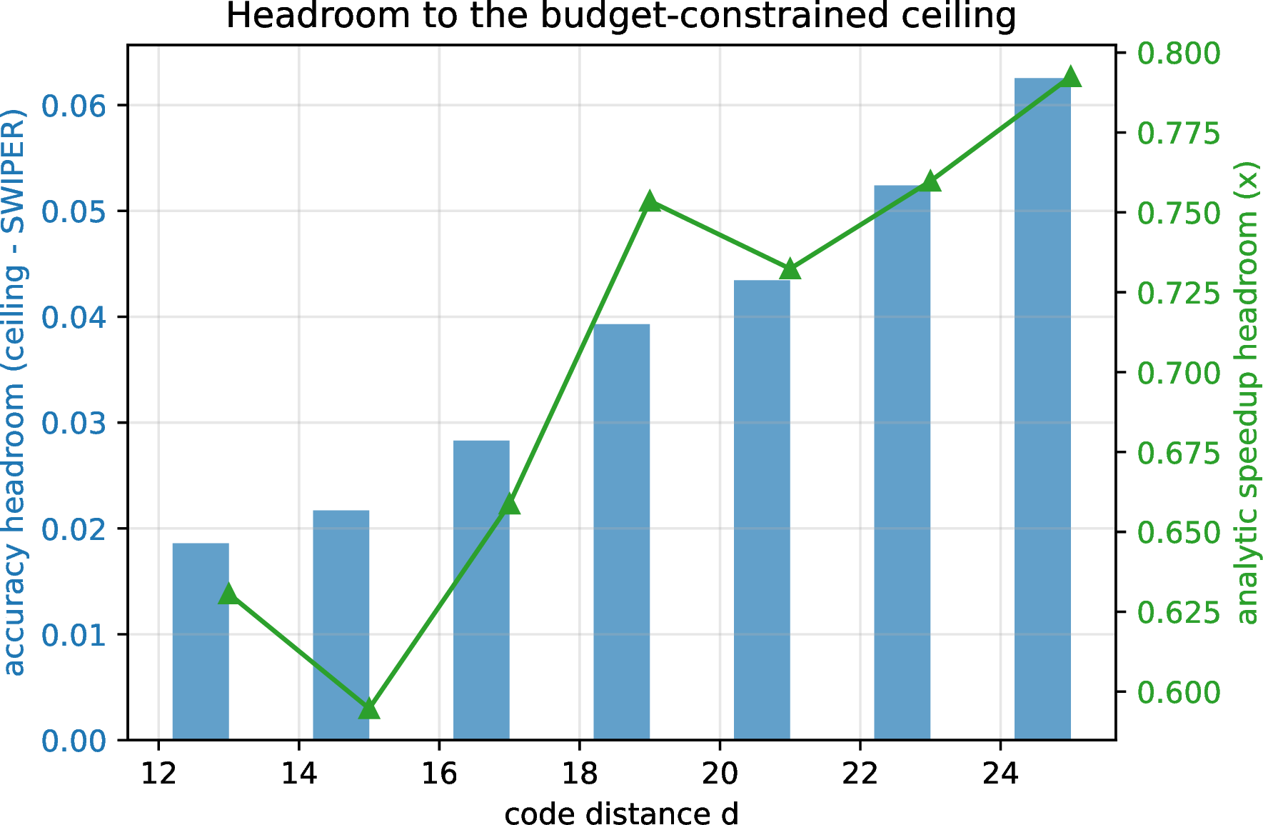
The headroom over SWIPER is real but modest, and it grows with distance. At SWIPER’s own receptive field the achievable accuracy exceeds the reported three-step predictor by \(0.019\) at \(d=13\), rising to \(0.063\) at \(d=25\). Mapped to a speedup through the speculative-decoding formula of Leviathan et al. [9], with acceptance rate \(\alpha\) equal to the boundary accuracy and cost ratio \(c\) equal to predictor over decoder cost, that is a relative improvement of \(1.19\times\) at \(d=13\) to \(1.33\times\) at \(d=25\), reported as a band over \(c\in[0.05,0.5]\). This map assumes linear-chain rollback and a free speculation depth \(\gamma\le 32\), so the ratios are optimistic in absolute terms; the robust quantity is the ratio through the identical map, and the gap to the true graph-structured rollback is exactly the blast radius of Sec. 4.
That headroom is diffuse, not concentrated. The per-boundary-node error of the budget predictor is small (mean \(5\times10^{-5}\) at \(d=21\)) and uncorrelated with the pre-registered structural feature, distance to the spatial code boundary (correlation \(+0.04\)). The exact-match gap is the compounding of a per-bit gap of order \(10^{-4}\) over hundreds of bits, not a characterizable hard subset of boundaries. A smarter cheap predictor buys a few diffuse points; the actionable accuracy lever is one more round of receptive field. Per-bit predictability is near-saturated, which points the contribution at the recovery cost, the next section.
4 Bound, refute, and explain: the misprediction blast radius↩︎
4.1 The temporal containment bound↩︎
A misprediction passes wrong dependency bits into a window. The blast-radius question is whether that corruption propagates: does the wrong incoming boundary change the window’s outgoing boundary, and so poison the next window? We model exactly that operator on a single window with open temporal ends: perturb the incoming (sink) boundary, re-decode with MWPM, and read the change in the outgoing dependency bits at the cut, \(W\) rounds away.
We first fix the adversary class, before any bound, so that the result is neither vacuous nor trivial. The class \(\mathcal{A}(K,\Lambda)\) flips at most \(K\) sink bits within a
spacetime ball of diameter \(\Lambda\), placed worst-case (wrong precisely where the boundary was least predictable). Calibration from Sec. 3 sets the parameters rather than assuming them:
only \(0.3\%\) to \(0.6\%\) of boundaries are mispredicted, a poisoned boundary carries on average \(1.04\) wrong bits, and the maximum over \(d=7\) to \(11\) is \(K=3\). We bound this class above by flip_all, every sink bit flipped, which is verified to dominate the localized budget-\(K\) clusters empirically, so containment for flip_all implies containment for the hard-syndrome-correlated adversary.
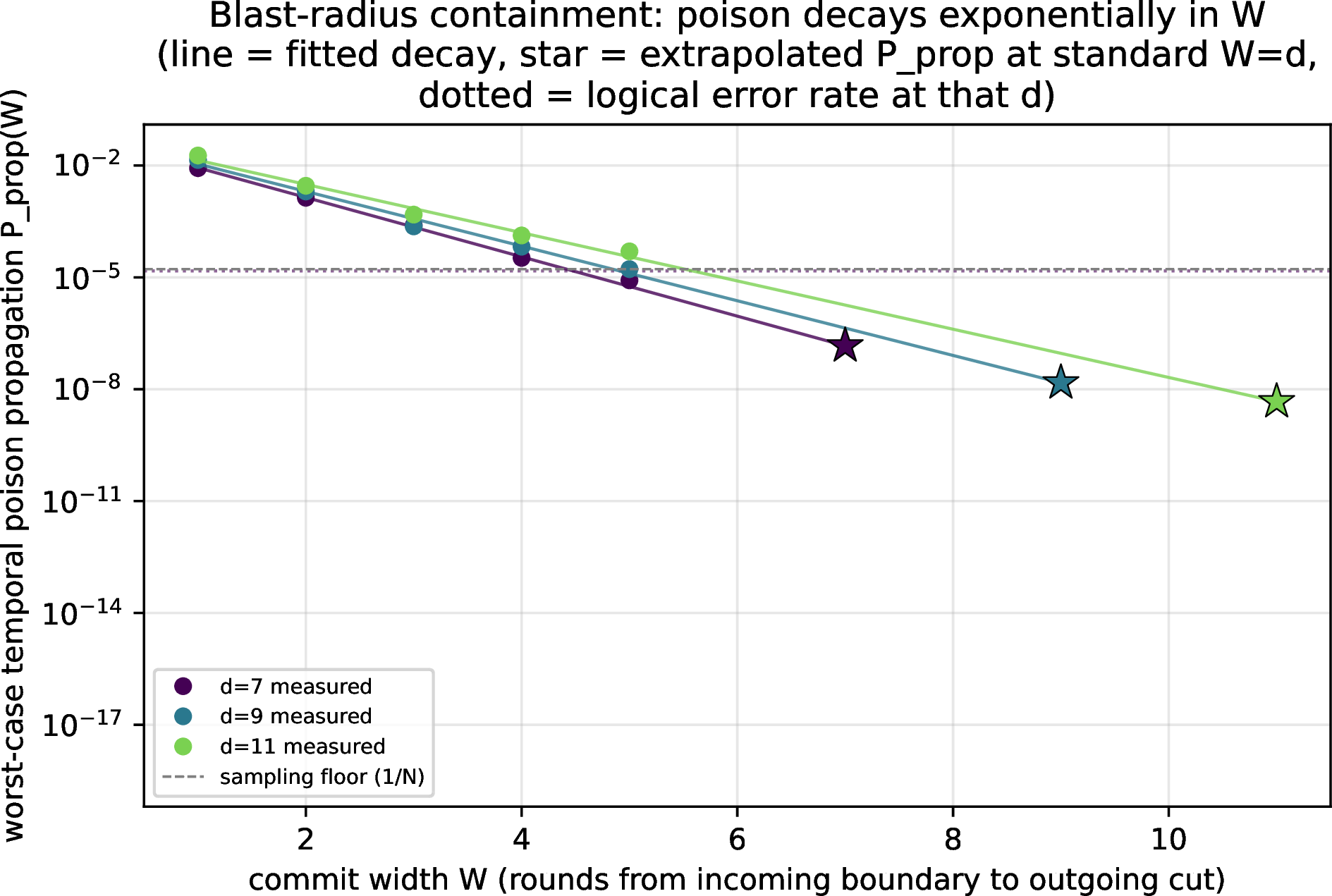
The finding is that the corruption is contained to the poisoned window. The propagation probability decays exponentially in the commit width \(W\), \[P_{\mathrm{prop}}(W)\;\le\;C\, d^2\, \lambda^{W}, \qquad \lambda = \sqrt{\deg^2\, c\, p} < 1, \label{eq:bound}\tag{1}\] with \(\deg=6\) the degree of an interior node in the rotated surface-code matching graph (four spatial and two temporal neighbors [15]) and \(c\) an order-one counting constant. The measured rate is \(\lambda = 0.16, 0.19, 0.23\) at \(d=7,9,11\) (\(p=10^{-3}\)), each below the conservative rigorous rate \(0.38<1\), and the prefactor scales as \(d^2\) (Fig. 3). At the standard commit width \(W=d\) the failure probability is \(1.5\times10^{-7}\), \(1.5\times10^{-8}\), \(4.7\times10^{-9}\) at \(d=7,9,11\). For comparison, the \(d\)-round logical error rate measured on the same harness is \(1.5\times10^{-5}\) at \(d=7\) (below the resolution of our shot count for \(d\ge 9\)), so at \(d=7\) the propagation sits two orders of magnitude below it, and \(P_{\mathrm{prop}}(W=d)\) falls faster in \(d\) (as \(\lambda^{d}\)) than the logical error rate. The temporal blast radius is one, and verified speculation adds no error floor.
4.2 Machine-checked core, certified reduction↩︎
We keep the line between proven and empirical explicit. The probability machinery is machine-checked in Lean 4 with Mathlib [16]: the development builds
with no sorry, and #print axioms on the assembled theorem reports only the three standard axioms (propositional extensionality, choice, quotient soundness). What Lean proves is the Peierls/union-bound tail (the probability that
some boundary-to-cut path is entirely faulty is at most the path count times \(q^m\)), the assembled containment statement (under a reduction and a path-count bound, the propagation probability is at most \(B\,q^{W}\)), the subsidized \(q^{W/2}\) rate, and the path-count bound itself (at most \(\deg^{W}\), proved with an automated prover). This is the machinery that
makes the bound exponential, with the rate and the constant pinned.
What is not proved from the decoder, and is carried as an explicit hypothesis backed by the empirical certificate of Eq. 1 , is the reduction itself: that poison reaching the cut implies a faulty boundary-to-cut path of length at least \(W\), together with the surface-code constants. The clean deterministic version of that reduction (a weight-\(K\) perturbation confines its effect within graph distance \(K\)) is false under noise, since a single flipped sink bit changes the outgoing boundary at distance two or three by riding background error chains, which is why the statement must be probabilistic. That probabilistic form is exactly what the Lean tail bound consumes.
4.3 Both halves of SWIPER’s observation↩︎
SWIPER reports no degradation between non-adjacent boundaries and about \(4\%\) between adjacent ones. The temporal result above is the first half (non-adjacent, about \(10^{-7}\)). For the second half we build a corner window with a spatial cut and a temporal cut meeting at a corner, perturb the spatial face, and measure the temporal face. The coupling is a bounded constant of a few percent (\(4.96\%\), \(5.36\%\), \(6.42\%\) at \(d=9,11,13\), against SWIPER’s \(4\%\)), invariant to the commit width, and corner-localized: a single spatial row perturbed at distance \(\delta\) from the corner couples as roughly \(\exp(-c\,\delta)\). The two faces meet at an order-one distance, so the coupling is a constant rather than the \(\exp(-cW)\) of the temporal direction. This reproduces and explains why adjacent is about \(4\%\) and non-adjacent is about zero, and justifies the “restart poisoned plus adjacent” policy. We characterize this coupling but do not prove a containment bound for it, unlike the temporal direction (Sec. 8).
4.4 Refuting the reduction, and the real mechanism↩︎
The Lean core is conditional on the reduction hypothesis, certified only in aggregate. We test it shot by shot. From the same decomposed detector error model the decoder matches against, we extract each shot’s ground-truth faults, anchored by an exact identity: the parity of a shot’s fired-fault detector components equals Stim’s sampled syndrome, so the fault set is ground truth, not an inference. A pre-registered battery of candidate necessary-structure predicates, the two literal forms of the Lean hypothesis plus variants from three independent lenses (percolation, matching cost, graph cut), is then searched for counterexamples: a shot that propagates while the predicate is false refutes that predicate as a necessary condition.
The falsification deliberately sharpens the adversary. The bound of Sec. 4 uses flip_all as a worst-case upper bound; to hunt counterexamples we instead use a single flipped sink bit, the sharpest probe of
whether one wrong bit needs a faulty path to propagate. Under it every candidate is refuted (Table 1). The canonical reduction (undirected all-faulty connectivity from the flip to the cut) survives only \(0.071\) of propagating shots (\(23{,}934\) counterexamples), and essentially none at commit width two or more; the \(q^{W/2}\) subsidy refinement survives a
minority; only the vacuous floor (some fault present somewhere in the band) survives (Table 1). Propagation routinely occurs with no faulty path anywhere near the flipped bit. The faulty-path route to formalizing the
reduction is therefore closed. (Under flip_all the same reduction survives \(0.52\), which is why an aggregate certificate alone does not expose the gap.)
| Predicate | Structural content | Survival |
|---|---|---|
| flow2_faulty | \(\ge 2\) disjoint faulty sink\(\to\)cut paths | \(0.000\) |
| reach_all_oriented | monotone all-faulty sink\(\to\)cut path | \(0.068\) |
| reach_all\(^\star\) | undirected all-faulty connectivity (canonical) | \(0.071\) |
| subsidy_half\(^\star\) | length-\(W\) path with \(\ge\lceil W/2\rceil\) faulty edges | \(0.256\) |
| weighted_subsidy | subsidised crossing \(\le\) boundary-absorb cost | \(0.488\) |
| layer_cover | faulty cluster crosses every layer (Peierls) | \(0.071\) |
| fault_near_flip_r2 | faulty edge within graph distance 2 of flip | \(0.501\) |
| fault_near_flip_r0 | flip incident to a faulty edge | \(0.060\) |
| any_faulty | any faulty band edge (vacuous floor) | \(1.000\) |
A re-pairing instrument then demonstrates the real mechanism (Table 2). Decoding twice (baseline and single-bit flip) and taking the symmetric difference of the matched edge sets gives the change in the correction. On propagating shots that change is a long re-route that reaches the cut depth (\(98.8\%\) of the time) carrying no faulty flip-to-cut path (\(99.5\%\) of the time), while on non-propagating shots it is a single edge, a local absorb at the boundary. The crossing is cheaper than the absorb: the re-route re-pairs an existing cut-region defect with the flipped bit, recouping that defect’s matching cost. Propagation is a global minimum-weight re-pairing, not faulty-path percolation. The per-rate breakdown matters and the pooled medians are confounded, since \(94\%\) of propagating events occur at \(p=10^{-2}\): the direction, a longer re-route at smaller matching weight reaching the cut with no faulty path, holds at every \(p\). The mechanism is partly degeneracy-driven, and increasingly so with \(p\): the fraction of decisions that flip under a small weight perturbation rises from \(0.04\) at \(p=10^{-3}\) to \(0.40\) at \(p=10^{-2}\), so at high noise the re-pairing is frequently a near-tie while at low noise it is a cleaner but far rarer win. The low-\(p\) row rests on only \(24\) propagating events and is indicative.
| \(p\) | \(n_{\mathrm{prop}}\) | symdiff (p / np) | \(\Delta w\) (p / np) | reaches cut | no faulty path | tie-sensitive |
|---|---|---|---|---|---|---|
| \(10^{-3}\) | 24 | 5 / 1 | 3.17 / 5.05 | \(1.000\) | \(1.000\) | \(0.04\) |
| \(3\times10^{-3}\) | 348 | 6 / 1 | 2.48 / 3.95 | \(0.971\) | \(0.994\) | \(0.13\) |
| \(10^{-2}\) | 5771 | 11 / 1 | 1.41 / 2.44 | \(0.989\) | \(0.995\) | \(0.40\) |
None of this touches the Lean core, which is a correct conditional theorem. What is falsified is the hypothesis it is conditional on, so the exponential containment is real but is not explained by faulty-path percolation. The correct future bound is a statement about matching weight: propagation needs \(\Omega(W)\) subsidy to beat the local absorb over \(W\) rounds, which is plausibly the source of the measured \(P_{\mathrm{prop}}\sim\lambda^{W}\) but is not proved here (Sec. 8).
5 Decide: the speculation-decision pass↩︎
To make the physical blast-radius bounds and predictability limits actionable for a runtime software stack, we abstract them into a compiler pass. The two numbers above feed a compiler decision. We work at the level the decision lives, an abstract window dependency graph, with windows on a space-by-time grid and dependencies typed temporal or spatial. This graph makes no assumption about physical qubit topology or proprietary control hardware: it captures only the window-to-window commit dependencies, so the pass is portable across code layouts and control stacks. A front end that lowers a routed program to this graph is a thin future adapter and is not needed to make the decision. A transpiler pass annotates each boundary with a speculate flag from the cost model \[\mathrm{cost} = \mathrm{predictability}\times\mathrm{slack} - \mathrm{blast\_radius},\] wiring the real head-A predictability (\(0.992\) at \(d=13\)) and the head-B couplings (temporal \(1.46\times10^{-7}\), spatial \(0.064\)), where the blast-radius term is the expected recovery cost and the restart set is itself derived from the couplings.
The pass derives SWIPER’s policy rather than hardcoding it: speculate on all boundaries, and on a misprediction restart the poisoned window (temporal radius zero) plus its corner-adjacent neighbor (spatial radius one). This holds for any restart threshold between the two couplings, a window of \(4.4\times10^{5}\), because the blast-radius work separated the temporal and spatial couplings by more than six orders of magnitude; a counterfactual that raises the temporal coupling to \(0.1\) expands the temporal restart radius to one, so the policy follows the numbers. On a mixed graph with a low-predictability region the cost model beats both speculate-everything and speculate-nothing.
6 Execute: the runtime executor↩︎
The decision is only a proxy until something executes it. A standalone executor takes the pass’s plan and runs predict, verify, and bounded-recover against the real harness, turning the cost-model proxy into a measurement. The latency model is stated and hardware-agnostic: each window decode costs \(L\), a non-speculated boundary forces its successor to wait (cost \(L\) on the critical path), and a speculated boundary starts immediately except for the expected restart, which carries the measured misprediction rate times the measured propagation rate. Makespan is the longest path over the window graph.
Recovery is exact and bounded (Table 3). Under a worst-case misprediction the committed decode is correct on every shot, over \(40{,}000\) shots per cell, because the lazy verify is the full decode and the bounded restart restores it. The recover loop converges in a single round: a radius-zero restart of the poisoned window suffices. The loop is bounded in its header, so termination is structural.
The measurement that matters is the restart penalty, since the speedup over no speculation on a chain of \(N\) windows is \(N\) up to that penalty by construction. The penalty is small: the per-boundary expected restart cost is the measured misprediction rate times the measured propagation rate, about \(1.3\times10^{-5}\), because mispredictions are rare and almost all are absorbed. On a chain of \(16\) windows this gives a speedup of \(15.99\) to \(16.00\) across distances and commit widths, holding even when predictability is degraded to \(0.7\) (Table 3), so the policy removes the per-window commit-chain stall up to a penalty of order \(10^{-5}\). The ideal for an \(N=16\) chain is exactly \(16\), every window’s commit-chain wait hidden, so the executor runs at \(99.9\%\) of the architecture’s theoretical limit, the residual being the restart penalty. This is the critical-path dependency latency, not a wall-clock runtime claim, which depends on the commit-chain fraction of total runtime (SWIPER’s regime).
| \(d\) | \(W\) | Restart rate | Speedup | Speedup (pred \(=0.7\)) | Recovery |
|---|---|---|---|---|---|
| 7 | 1 | \(8.9\times10^{-3}\) | \(15.999\) | \(15.80\) | exact |
| 7 | 2 | \(1.3\times10^{-3}\) | \(16.000\) | \(15.94\) | exact |
| 7 | 3 | \(1.0\times10^{-4}\) | \(16.000\) | \(15.99\) | exact |
| 7 | 4 | \(0\) | \(16.000\) | \(15.99\) | exact |
| 9 | 1 | \(1.3\times10^{-2}\) | \(15.997\) | \(15.81\) | exact |
| 9 | 2 | \(2.4\times10^{-3}\) | \(15.999\) | \(15.93\) | exact |
| 9 | 3 | \(3.2\times10^{-4}\) | \(16.000\) | \(15.99\) | exact |
| 9 | 4 | \(1.5\times10^{-4}\) | \(16.000\) | \(16.00\) | exact |
Executing the plan also corrects the cost model. The head-C blast-radius term assumes every misprediction restarts, but the executor measures that only the propagating fraction does, so the true expected restart cost is smaller by the propagation probability, a factor of \(10^{-3}\) at small commit width and \(10^{-7}\) at \(W=d\). At the real restart cost the corrected and proxy decisions agree and the head-C result stands; the gap opens only when restarts are made artificially expensive, where the proxy declines speculation prematurely (a speedup of \(1.78\times\) where \(14.5\times\) is available) and the corrected decision stays optimal. Folding the propagation probability into the cost model is a one-line refinement.
7 Decoder-relativity: what is decoder-agnostic↩︎
The contribution sits above the decoder, so we test which findings depend on the decoder. We build a second, algorithmically distinct decoder, the union-find decoder of Delfosse and Nickerson [17] (unweighted cluster growth and peeling), on the same matching graph the MWPM reference uses, so only the matching rule changes. It is validated first: every correction reproduces the syndrome exactly (node-degree parity equals syndrome on every shot), and the logical error rate suppresses with distance, tracking MWPM within a small factor. Because this union-find is unweighted its threshold is below MWPM’s, so the cross-decoder check is scoped to \(p\le 3\times10^{-3}\), the regime where it is a validated below-threshold decoder.
Two structural findings are decoder-robust (Fig. 4). The locality of the cut decision (Sec. 3) holds, checked here over \(d=9\) to \(13\): radius-\(R\) accuracy saturates near one by \(R=3\) under union-find as under MWPM, about one to two points noisier with the same shape. The refutation of the reduction (Sec. 4.4) holds: the reduction survives at most \(0.005\) of propagating shots at commit width two or more under union-find, and union-find propagates more events yet refutes at least as hard.

What is decoder-relative is the absolute predictability magnitude and the speedup ratios, which depend on the reference decoder’s per-bit accuracy, the rate constant \(\lambda\), and the minimum-weight re-pairing mechanism of Sec. 4.4, which is intrinsic to a minimum-weight decoder and so was deliberately not re-run under union-find. The precise statement is this: the predict/verify/recover wrapper is decoder-agnostic by construction, since any decoder plugs in behind the verify step and union-find does so unchanged; the phenomenology is decoder-robust at the level a runtime needs (locality, no-faulty-path propagation, radius one) and decoder-relative in its absolute numbers and in the min-weight explanatory mechanism.
8 Limitations and future work↩︎
The matching-weight bound. The falsification closed the faulty-path route to formalizing the reduction, and the mechanism study shows the correct statement is about matching weight: propagation needs \(\Omega(W)\) subsidy to beat the local absorb over \(W\) rounds. That is the natural source of the measured \(P_{\mathrm{prop}}\sim\lambda^{W}\), but it is not proved; it is the next formalization target and is out of scope here.
Sim-accurate speedup. The speedup numbers in Sec. 3 are the analytic linear-chain map with a free speculation depth. The graph-structured, restart-cost-accurate speedup needs the SWIPER-SIM pipeline, which is not public; that validation is future work and the natural contribution back to SWIPER-SIM.
Spatial blast radius. The corner coupling is characterized (a bounded few percent, corner-localized, width-invariant) but not bounded the way the temporal direction is.
Decoder-relativity envelope. Union-find is unweighted, so the cross-decoder check is scoped to \(p\le 3\times10^{-3}\). A weighted-growth union-find for higher \(p\), and a non-matching decoder with a redefined boundary readout, are future work. The min-weight mechanism is matching-specific by construction.
Harness reconstruction. SWIPER-SIM’s exact configuration is not public, so the harness is a documented reconstruction and all headroom is internal (predictor-versus-bracket on the same harness). A direct SWIPER-SIM cross-check is future work.
Bare-metal deployment. The executor here runs the predict-verify-recover loop in software against the harness, measuring critical-path dependency latency under a stated hardware-agnostic cost model. Deploying the same wrapper on a physical control kernel or an FPGA-based real-time decoding environment, where the round cadence and decode latency are set by hardware rather than modeled, would turn the critical-path result into a wall-clock one and is the natural next step.
9 Conclusion↩︎
The predictor half of speculative window decoding was built twice; the verifier half was open. We built it: a predictability bracket that shows the cross-boundary decision is local and SWIPER is near the achievable accuracy, a worst-case blast-radius bound with a machine-checked probability core that shows a wrong guess is contained to radius one and adds no error floor, a falsification and mechanism study that replaces the bound’s modeling hypothesis with a global minimum-weight re-pairing (demonstrated where propagation is common, at \(p=10^{-2}\), and directionally robust though on few events at lower noise), a compiler pass that derives SWIPER’s restart policy from these numbers, and a runtime executor that confirms on the real harness that the loop recovers exactly and removes the commit-chain stall up to a small restart penalty. The verifier side is a reusable layer that sits above any decoder; a second decoder confirms that the structural results are decoder-robust while the absolute magnitudes and the min-weight mechanism are specific to matching. The code, the machine-checked development, and every figure and table are reproducible from fixed seeds.
Code and data availability↩︎
The harness, predictors, blast-radius operator, compiler pass, runtime executor, union-find decoder, the Lean 4 development, and the scripts that regenerate every result, figure, and table from fixed seeds are available at https://codeberg.org/rylanmalarchick/speculative-qec.
Acknowledgments↩︎
The path-count bound in the Lean development was closed with the Aristotle automated prover.
AI Disclosure↩︎
AI-assisted tools (Claude, Anthropic) were used for code development, running the numerical experiments, and manuscript preparation. The research direction, design decisions, and interpretation are the author’s, who takes full intellectual responsibility for all content.