Automatic Differentiation from Scratch: How Pytorch Computes Gradients in Physics-Informed Neural Networks
June 13, 2026
Abstract
This paper traces, with explicit numerical values, how PyTorch’s automatic differentiation (AD) engine computes gradients for Physics-Informed Neural Network (PINN) training — a setting that requires two levels of differentiation: computing the physics
derivative \(\hat{y}'(t) = d\hat{y}/dt\) through the network, and computing parameter gradients \(\nabla_\theta L\) of a loss that itself depends on \(\hat{y}'(t)\). Using a 1-3-3-1 multilayer perceptron and the initial value problem \(y'(t) + y(t) = 0\), \(y(0) = 1\) from [1], we trace the complete pipeline at every node: the computational graph built during the forward
pass, the reverse-mode backward traversal that computes all 22 parameter gradients in a single pass, and the graph-on-graph mechanism by which create_graph=True enables correct differentiation through the physics-informed residual. Every
adjoint value is verified against the hand derivations of [1], connecting the
\(P/Q\) sensitivity framework to the vector–Jacobian products used by PyTorch’s autograd engine.
Keywords: automatic differentiation, reverse-mode automatic differentiation, backpropagation, computational graph, vector–Jacobian product, Physics-Informed Neural Networks, PyTorch
MSC codes: 65D25, 65-01, 68T07, 65L05
1 Introduction↩︎
A typical Physics-Informed Neural Network (PINN) training loop fits in fewer than twenty lines of PyTorch. The forward pass computes the network output \(\hat{y}(t;\theta)\); a call to torch.autograd.grad with create_graph=True computes the time derivative \(\hat{y}'(t)\); the ODE residual \(R = \hat{y}'+ \hat{y}\) is squared to form
the loss; and loss.backward() produces all parameter gradients in a single call. The entire pipeline relies on automatic differentiation (AD) — yet what does each of these calls actually compute, and why is each
flag necessary? Answering these questions requires opening the black box.
1.0.0.1 Two differentiation tasks.
Training a PINN requires two fundamentally different derivatives. Consider the first-order ODE \(y'(t) + y(t) = 0\) with initial condition \(y(0) = 1\). The PINN loss at a collocation point \(t_c\) is \[\label{eq:intro95loss} L = \underbrace{\left( \hat{y}(t_c;\theta) + \frac{\partial\hat{y}}{\partial t}\bigg|_{t_c} \right)^2}_{L_R:\;\text{ODE residual}} + \;\lambda\, \underbrace{\bigl(\hat{y}(0;\theta) - 1\bigr)^2}_{ L_{IC}:\;\text{initial condition}}.\tag{1}\] The loss involves the physics derivative \(\partial\hat{y}/\partial t\) — how the network output changes when the input \(t\) varies, with all parameters held fixed — and training requires a second derivative, the training gradient \(\nabla_\theta L\), which describes how the loss changes when a parameter \(\theta_k\) is adjusted. We write \(\hat{y}'\) for \(d\hat{y}/dt\); since the parameters \(\theta\) do not depend on \(t\), this coincides with \(\partial\hat{y}/\partial t\).
In standard supervised learning, the loss depends only on \(\hat{y}\), and a single backward pass computes \(\nabla_\theta L\). Here the loss depends on both \(\hat{y}\) and \(\hat{y}'\), so the training gradient of the residual loss is \[\label{eq:intro95grad}
\frac{\partial L_R}{\partial\theta_k}
= 2R\left( \frac{\partial\hat{y}}{\partial\theta_k} + \frac{\partial\hat{y}'}{\partial\theta_k}
\right).\tag{2}\] The second term \(\partial\hat{y}'/\partial\theta_k\) is the PINN-specific complication: a second-order mixed derivative \(\partial^2\hat{y}/
\partial\theta_k\,\partial t\) that requires differentiating the physics-derivative computation itself with respect to the parameters. In PyTorch, this term exists only if the physics derivative was computed with create_graph=True;
omitting the flag silently drops it, producing wrong gradients without any error message.
This ODE is the “hello-world” of physics-informed learning — small enough to admit closed-form analysis, yet rich enough to exhibit the two-derivative coupling above. A companion paper [1] develops the analytical derivation of the resulting training gradient for a 1-3-3-1 MLP applied to this problem; the present paper traces the corresponding machine computation inside PyTorch’s AD engine.
1.0.0.2 From hand-derived gradients to framework AD.
Training neural networks to satisfy differential equations predates modern deep learning. Early work by Dissanayake and Phan-Thien [2] and Lagaris et al. [3] derived the gradient expressions required for training analytically, for shallow architectures with fixed activation functions; the resulting formulas had to be re-derived whenever the architecture changed. The emergence of general-purpose AD inside deep-learning frameworks — in particular reverse-mode AD as exposed by PyTorch [4] — removed this constraint by computing both the physics derivatives (such as \(\partial\hat{y}/\partial t\)) and the parameter gradients \(\nabla_\theta L\) generically, regardless of network depth or activation choice. This shift made deep architectures tractable and enabled the modern PINN framework of Raissi et al. [5], in which boundary or initial conditions are enforced through additional loss terms, as well as concurrent neural-network PDE solvers such as the Deep Galerkin method [6] and the Deep Ritz method [7]. Since 2019, PINNs have been applied to fluid dynamics [8], inverse problems [9], and a broad range of scientific computing tasks [10], [11].
1.0.0.3 The pedagogical gap.
The theoretical foundations of AD are well established. Griewank and Walther [12] provide the definitive treatment of forward and reverse modes; Baydin et al. [13] survey the field for a machine learning audience; standard textbooks [14] cover backpropagation, the application of reverse-mode AD to neural network training, following Rumelhart et al. [15]. On the PINN side, introductory treatments such as Katsikis et al. [16] explain the loss formulation and training methodology, while peer-reviewed didactic derivations such as Blechschmidt and Ernst [17] work through the residual symbolically by chain rule on a single-hidden-layer network — stopping short of the AD engine itself. What is missing is the bridge between the analytical derivation and the machine computation: a single document that traces, at the level of individual operations and explicit numerical values, how the AD engine handles the two-derivative coupling of 1 2 on a multi-layer network. Specifically:
What data structure does PyTorch build during the forward pass?
How does a single backward traversal compute all 22 parameter gradients simultaneously?
What does
create_graph=Trueactually do, and why does omitting it silently produce wrong gradients?How do the adjoint vectors propagated by PyTorch relate to the \(P/Q\) sensitivities derived by hand in [1]?
Existing references address pieces of this story — AD theory without PINN specifics, PINN formulations without AD internals — but none assembles them into a single, verifiable narrative on a worked example. Closing this gap prevents silent implementation errors, clarifies the computational cost of physics-informed training, and provides the foundation for developing techniques that improve convergence and accuracy.
1.0.0.4 What this paper covers.
We trace the complete AD pipeline for the same 1-3-3-1 MLP and the same IVP \(y' + y = 0\), \(y(0) = 1\) used in [1]. This pairing is small enough that every intermediate quantity — the activations of the forward
pass, the 22 parameter gradients of the backward pass, and the extended graph created by create_graph=True — can be displayed explicitly, yet large enough that the two-derivative coupling of 1 2 appears in full generality:
2 introduces tangent and adjoint vectors on a minimal two-input composition.
3 traces the forward pass of the 1-3-3-1 MLP and catalogues the computational graph.
4 traces the backward pass node by node, computing all 22 parameter gradients in one traversal.
5 explains the graph-on-graph: how
create_graph=Trueenables correct training gradients, including the product rule and \(\phi''\) terms.6 addresses common pitfalls, memory, and implementation patterns.
Every intermediate value is verified against the hand derivations of [1] and against PyTorch’s output; a companion Jupyter notebook reproduces all calculations. The physics derivative \(\hat{y}'\) can also be computed by forward-mode AD — during the forward pass, a tangent vector \(\dot{a}^{(\ell)}\) is carried alongside each activation and updated by the local Jacobian at each layer, exactly the dual propagation in the forward-pass tables of [1] — and PyTorch supports this via torch.func.jvp. We trace the reverse-mode approach because it is the PyTorch default for PINN training. This paper does not propose a new PINN methodology, benchmark training strategies, or compare AD systems; its contribution is explanatory.
2 Tangents and Adjoints: The Two Faces of the Chain Rule↩︎
Automatic differentiation (AD) is a family of algorithms that compute derivatives by decomposing a computation into elementary operations and applying the chain rule systematically. PyTorch records these operations in a data structure called the computational graph. Before tracing derivatives through a neural network, we introduce the forward pass, forward-mode AD, backward-mode AD, and the graph-on-graph mechanism on a scalar function of two inputs — the smallest example that contains every ingredient PINN training needs.
2.1 A Minimal Example↩︎
Let \(y = f(g(x_1, x_2))\) with: \[\label{eq:fg95def} g(x_1, x_2) = 2x_1 + x_2, \qquad f(u) = u^2.\tag{3}\] At \(x_1 = 2\), \(x_2 = 1\): \[\label{eq:fg95values} u = g(2,1) = 5, \qquad y = f(5) = 25.\tag{4}\] The local derivatives are: \[\label{eq:fg95locals} \frac{\partial g}{\partial x_1} = 2, \qquad \frac{\partial g}{\partial x_2} = 1, \qquad f'(u) = 2u = 10.\tag{5}\] By the chain rule, \(\partial y/\partial x_1 = 10 \cdot 2 = 20\) and \(\partial y/\partial x_2 = 10 \cdot 1 = 10\). We first compute \(y = 25\) and trace what PyTorch records, then compute these derivatives in two ways that correspond to the two modes of automatic differentiation.
2.2 The Forward Pass and Graph 1↩︎
The forward pass computes \(y = 25\) by evaluating the operations in sequence: \(u = 2x_1 + x_2 = 5\), then \(y = u^2 = 25\). When an input has
requires_grad=True, PyTorch builds a computational graph that records this sequence. Each operation becomes a node in the graph — a record containing:
the operation performed and the numerical result (the primal value),
links to the input nodes and the Jacobian entries (gradient function
grad_fn) required to compute the derivative during the backward pass.
1 shows Graph 1 built during this forward pass.

Graph 1 is the recipe for computing derivatives: it stores the operations and the numerical values needed to evaluate local derivatives during a derivative pass. No input is perturbed (as in finite differences), and no symbolic formula is manipulated — the graph is a trace of elementary operations, each paired with a known, exact derivative rule.
2.3 Forward-Mode AD: Propagating a Tangent↩︎
Forward-mode AD computes derivatives by propagating a tangent vector \(\dot{\mathbf{x}}\) from the inputs through the computational graph. By seeding the input with a vector \(\mathbf{v} = (\dot{x}_1, \dot{x}_2)\), which can be viewed as \(d\mathbf{x}/d\lambda\) for an independent parameter \(\lambda\), the derivative is computed at each node via the rule: \[\dot{\text{output}} = J_{\text{local}} \cdot \dot{\text{input}}\]
This operation is a Jacobian–vector product (JVP), where the \(m \times n\) Jacobian left-multiplies an \(n \times 1\) tangent vector. This preserves the flow of data, mapping the \(n\) input perturbations to \(m\) output tangents. In the transition from inputs to node \(u\), the \(1 \times 2\) Jacobian \(J_u = [\partial u/\partial x_1, \partial u/\partial x_2]\) multiplies the \(2 \times 1\) tangent \((\dot{x}_1, \dot{x}_2)^\top\) to produce the scalar tangent \(\dot{u}\).
The final result \(\dot{y}\) represents the directional derivative of \(y\) in the direction of the seed \(\mathbf{v}\), scaled by its magnitude. Specifically, choosing the standard basis vector \(e_i\) as the seed recovers the partial derivative \(\partial y / \partial x_i\).
1 traces the two passes needed to obtain both partial derivatives.
| Step | Pass 1: \(\dot{x}_1\!=\!1,\; \dot{x}_2\!=\!0\) | Pass 2: \(\dot{x}_1\!=\!0,\; \dot{x}_2\!=\!1\) |
|---|---|---|
| At node \(u\): \(\dot{u} = 2\dot{x}_1 + 1\cdot\dot{x}_2\) | \(2 \cdot 1 + 1 \cdot 0 = 2\) | \(2 \cdot 0 + 1 \cdot 1 = 1\) |
| At node \(y\): \(\dot{y} = f'(u)\cdot\dot{u} = 10\,\dot{u}\) | \(10 \cdot 2 = 20\;✔\) | \(10 \cdot 1 = 10\;✔\) |
2 shows the two passes through Graph 1. Tangent values (green, bold) are shown inside each node. Pass 1 seeds \(\dot{x}_1 = 1, \dot{x}_2 = 0\) and produces \(\dot{y} = 20 = \partial y/\partial x_1\). Pass 2 seeds \(\dot{x}_1 = 0, \dot{x}_2 = 1\) and produces \(\dot{y} = 10 = \partial y/\partial x_2\).
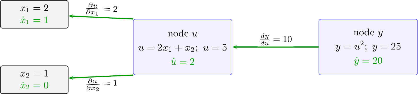
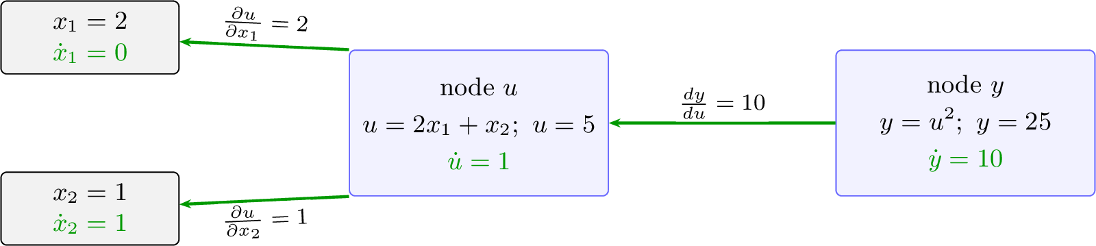
Figure 2: Graph 1 traversed in forward mode. Top: Pass 1 with seed \(\dot{x}_1 = 1, \dot{x}_2 = 0\). Bottom: Pass 2 with seed \(\dot{x}_1 = 0, \dot{x}_2 = 1\)..
2.4 Backward-Mode AD: Propagating an Adjoint↩︎
Backward-mode AD utilizes the computational graph to compute derivatives by propagating an adjoint from the output back to the inputs. The process begins at the output with a seed \(\bar{y} = dy/dy = 1\). At each node, the adjoint is propagated backward according to the rule: \[\bar{\text{input}} = \bar{\text{output}} \cdot J_{\text{local}}\]
This is a vector–Jacobian product (VJP). To propagate sensitivities backward, the \(1 \times m\) adjoint left-multiplies the \(m \times n\) Jacobian. This order is dimensionally required to "pull" the sensitivity of the \(m\) outputs back to the \(n\) inputs, resulting in a \(1 \times n\) adjoint vector. Projecting this to our example, the scalar adjoint \(\bar{u}\) (a \(1 \times 1\) vector) multiplies the \(1 \times 2\) Jacobian \(J_u\) to simultaneously "distribute" the sensitivity to both \(\bar{x}_1\) and \(\bar{x}_2\) in a \(1 \times 2\) row.
Here, the overbar notation \(\bar{v} = \partial y / \partial v\) denotes the adjoint of \(v\), representing the sensitivity of the final output \(y\) with respect to the intermediate variable \(v\). Unlike forward-mode, a single backward pass efficiently recovers the gradient of the output with respect to all input parameters simultaneously.
2 traces the single pass.
| Step | VJP rule | Result |
|---|---|---|
| Seed | \(\bar{y} = 1\) | \(1\) |
| At node \(y\): \(\bar{u} = \bar{y} \cdot f'(u)\) | \(1 \cdot 10\) | \(10\) |
| At node \(u\): \(\bar{x}_1 = \bar{u} \cdot \partial g/\partial x_1\) | \(10 \cdot 2\) | \(20\;✔\) |
| At node \(u\): \(\bar{x}_2 = \bar{u} \cdot \partial g/\partial x_2\) | \(10 \cdot 1\) | \(10\;✔\) |
One pass produced both \(\partial y/\partial x_1 = 20\) and \(\partial y/\partial x_2 = 10\), plus the intermediate adjoint \(\bar{u} = 10\).
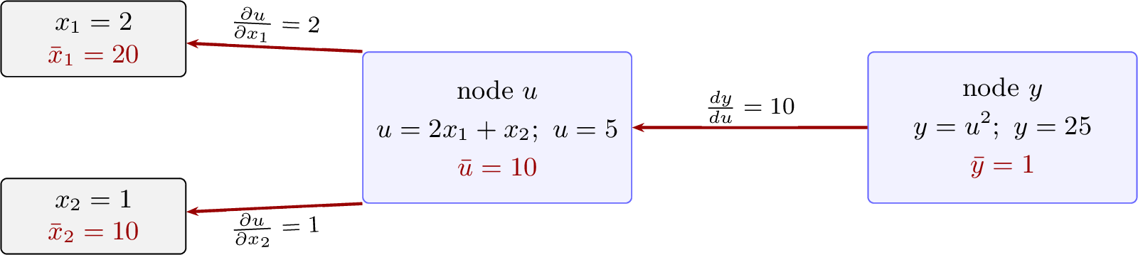
3 shows the same Graph 1 traversed in backward mode. The adjoint seed \(\bar{y} = 1\) starts at the output node and flows right to left. At each node, the incoming adjoint is multiplied by the local derivative on each outgoing edge to produce the adjoint at the next node: \(\bar{u} = \bar{y} \cdot 10 = 10\), then \(\bar{x}_1 = \bar{u} \cdot 2 = 20\) and \(\bar{x}_2 = \bar{u} \cdot 1 = 10\).
2.4.0.1 The key distinction.
Both modes apply the same local derivatives (\(f' = 10\), \(\partial g/\partial x_1 = 2\), \(\partial g/\partial x_2 = 1\)). They differ in direction and cost:
| Forward-mode (JVP) | Backward-mode (VJP) | |
|---|---|---|
| Direction | input \(\to\) output | output \(\to\) input |
| Local rule | \(\dot{y} = J \cdot \dot{x}\) | \(\bar{x} = \bar{y} \cdot J\) |
| One pass gives | \(\partial y/\partial x_i\) for one \(i\) | \(\partial y/\partial x_i\) for all \(i\) |
| Cost for \(n\) inputs, \(m\) outputs | \(n\) passes | \(m\) passes |
| Our example (\(n\!=\!2\), \(m\!=\!1\)) | 2 passes | 1 pass |
For any gradient-based optimization involving a scalar loss and a high-dimensional parameter space (\(m = 1, n \gg 1\)), backward-mode AD is significantly more efficient as it computes the full gradient \(\nabla y \in \mathbb{R}^n\) in a single backward pass. This computational advantage is the reason PyTorch adopts backward-mode as its default autodiff engine and provides the loss.backward() interface for gradient
calculation.
2.5 Second Order Derivative and the Graph-on-Graph Mechanism↩︎
The backward pass computed \(\bar{x}_1 = 20\) through VJP operations: \(\bar{u} = \bar{y} \cdot 2u = 10\), then \(\bar{x}_1 = \bar{u} \cdot 2 = 20\).
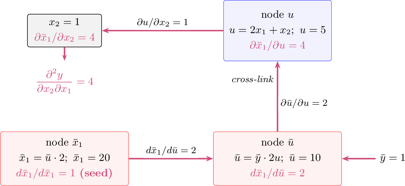
These VJP operations are themselves arithmetic. With create_graph=True, PyTorch records them in a second graph (Graph 2), making it possible to differentiate \(\bar{x}_1\) with respect to the original inputs.
4 shows both graphs: Graph 1 (top) built during the forward pass, and Graph 2 (bottom) built during the first backward pass. The dashed cross-link records that the VJP at \(y\) reads \(u = 5\) from Graph 1.
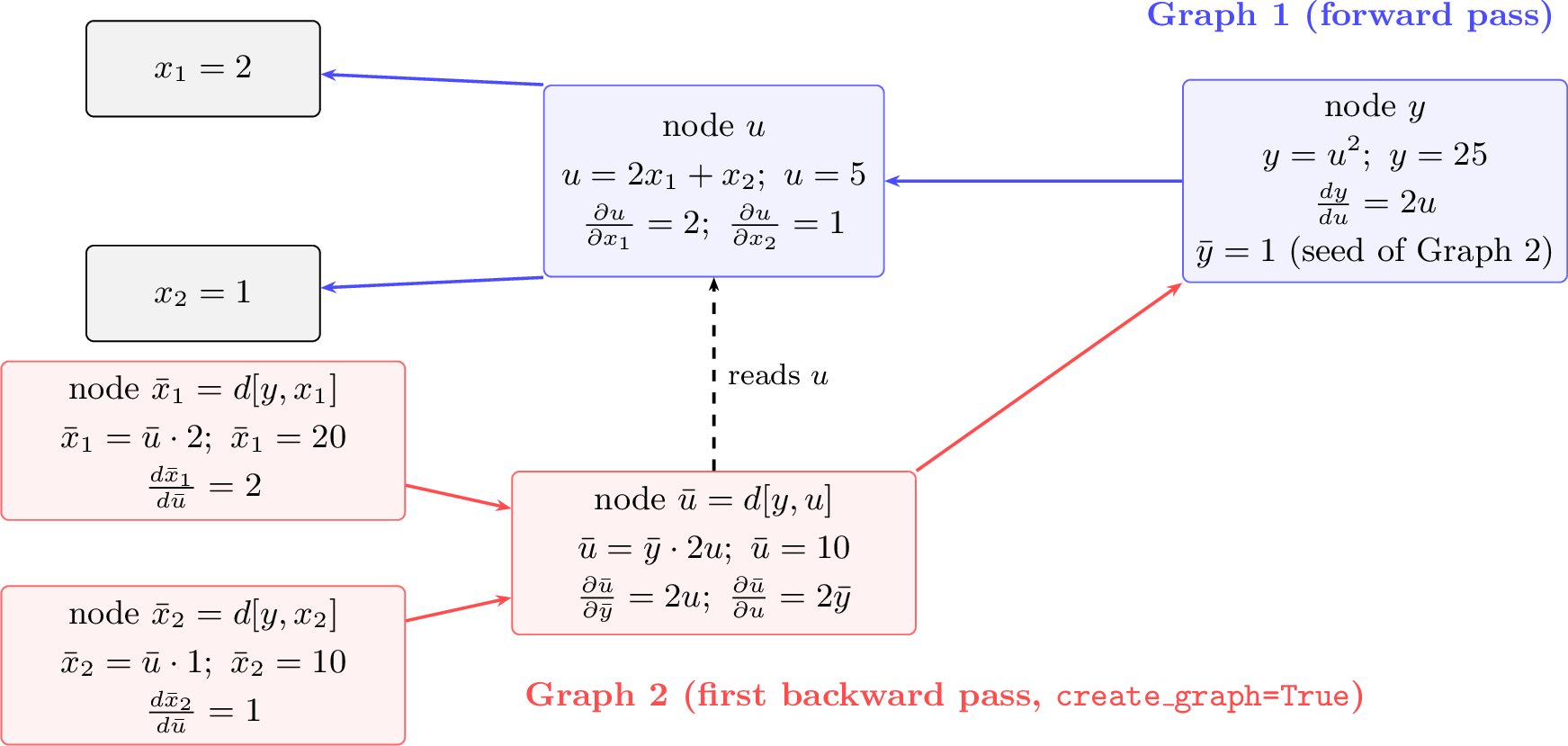
Without create_graph=True, the VJP operations execute but are not recorded. The mixed derivative becomes \(\partial\bar{x}_1/\partial x_2 = \partial(20)/\partial x_2 = 0\) (wrong; correct answer is 4).
5 shows the traversal propagating the adjoint from \(\bar{x}_1\) node with seed \(1\) back to \(x_2\) as a sequence of node visits, with the adjoint accumulating from 1 to 4 as it flows through the combined graph \(Graph\,1 + Graph\,2\).
2.5.0.1 The PINN analogy.
The roles in PINN training for the initial value problem presented in 3.1 map directly onto this example:
| Simple example | PINN |
|---|---|
| \(x_1\) | time \(t\) or network weight or bias \(\theta\) |
| \(x_2\) | \(\theta\) |
| \(\bar{x}_1 = \partial \hat{y}/\partial x_1\) | \(\hat{y}'= \partial \hat{y}/\partial t\) or \({\partial\hat{y}}/{\partial\theta}\) |
| \({\partial\bar{x}_1}/{\partial x_2}\) (second backward) | \({\partial\hat{y}'}/{\partial\theta}\) (needed for the residual loss) |
| Cross-link (VJP at \(y\) uses \(u\)) | Cross-links (VJP nodes use \(W^{(\ell)}\), \(a^{(\ell)}\)) |
2.6 Verification in PyTorch↩︎
To verify the theoretical framework, the following listings demonstrate PyTorch’s tiered approach to automatic differentiation, progressing from a standard forward pass to the computation of second-order mixed derivatives. While Level 0 ignores gradient
tracking, Level 1 allows for first-order gradients for the leaf tensors having requires_grad=True. The use of retain_graph=True in the first backward AD traversal is essential because PyTorch’s default behavior is to free the
intermediate buffers once a backward pass is completed; without this flag, the computation graph would be destroyed after calculating \(\bar{x}_1\), making the subsequent calculation of \(\bar{x}_2\) impossible. Level 2 utilizes create_graph=True to build a graph capable of tracking the second order derivatives — the derivatives of \(\bar{x}_1 = \partial y/\partial
x_1\).
import torch

x1 = torch.tensor(2.0)
x2 = torch.tensor(1.0)

u = 2 * x1 + x2
y = u ** 2

print(y.item())               #>>> 25.0
print(y.grad_fn)              #>>> None
x1 = torch.tensor(2.0, requires_grad=True)
x2 = torch.tensor(1.0, requires_grad=True)
u = 2 * x1 + x2
y = u ** 2
# Backward AD: x1 <- y and x2 <- y (the partial derivatives)
bar_x1 = torch.autograd.grad(y, x1,
retain_graph=True)[0]
bar_x2 = torch.autograd.grad(y, x2)[0]
print(bar_x1.item()) #>>> 20.0
print(bar_x2.item()) #>>> 10.0
print(bar_x1.grad_fn) #>>> None
# Let's try the traversal x2 <- bar_x1 (the mixed derivative)
try:
torch.autograd.grad(bar_x1, x2)
except RuntimeError as e:
print(e)
#>>> element 0 of tensors does not require grad
#>>> and does not have a grad_fnx1 = torch.tensor(2.0, requires_grad=True)
x2 = torch.tensor(1.0, requires_grad=True)
u = 2 * x1 + x2
y = u ** 2
# traversal x1 <- y
bar_x1 = torch.autograd.grad(y, x1,
create_graph=True)[0]
print(bar_x1.item()) #>>> 20.0
print(type(bar_x1.grad_fn).__name__) #>>> MulBackward0
mixed = torch.autograd.grad(bar_x1, x2)[0]
print(mixed.item()) #>>> 4.0With the mechanics of higher-order AD established, we are ready to apply these concepts to the development of a Physics-Informed Neural Network (PINN) model designed to solve a fundamental initial value problem.
3 The Forward Pass↩︎
We now move from the two-input composition to a real neural network. This section defines the problem and the network that will serve as our running example for the rest of the paper, computes the forward pass with explicit numerical values, and traces the computational graph that PyTorch builds along the way.
3.1 The Problem↩︎
We seek to approximate the solution of the initial value problem \[\label{eq:ode} y'(t) + y(t) = 0, \qquad y(0) = 1,\tag{6}\] whose analytical solution is \(y(t) = e^{-t}\). A Physics-Informed Neural Network (PINN) approximates \(y(t)\) by a neural network \(\hat{y}(t;\theta)\) and trains it by minimizing a loss function that penalizes the ODE residual \(R(t) = \hat{y}'(t) + \hat{y}(t)\) at collocation points and the initial condition error \(\hat{y}(0) - 1\). The details of the loss will be needed in 5; for now, the key point is that the loss depends on both \(\hat{y}\) and its derivative \(\hat{y}'= d\hat{y}/dt\), and the AD engine must handle both.
3.2 The Network↩︎
The network is a 1-3-3-1 multilayer perceptron: one input (\(t\)), two hidden layers with 3 neurons each using \(\tanh\) activation, and one linear output neuron producing \(\hat{y}(t)\). The forward pass through layer \(\ell\) is: \[\label{eq:layer95forward} z^{(\ell)} = W^{(\ell)} a^{(\ell-1)} + b^{(\ell)}, \qquad a^{(\ell)} = \phi(z^{(\ell)}),\tag{7}\] where \(\phi = \tanh\) for hidden layers and \(\phi = \text{identity}\) for the output layer. The network has 22 trainable parameters: \(\theta = \{W^{(\ell)}, b^{(\ell)}\}_{\ell=1}^{3}\).
We fix all parameters to enable hand verification. 3 lists the complete parameter set.
| Layer | Weights | Biases |
|---|---|---|
| \(\ell = 1\) (\(1 \to 3\)) | \(W^{(1)} = \begin{pmatrix} 0.2 \\ -0.5 \\ 0.8 \end{pmatrix}\) | \(b^{(1)} = \begin{pmatrix} -0.1 \\ 0.3 \\ -0.2 \end{pmatrix}\) |
| \(\ell = 2\) (\(3 \to 3\)) | \(W^{(2)} = \begin{pmatrix} 0.1 & -0.3 & 0.5 \\ 0.6 & 0.2 & -0.4 \\ -0.2 & 0.7 & 0.1 \end{pmatrix}\) | \(b^{(2)} = \begin{pmatrix} 0.2 \\ -0.1 \\ 0.4 \end{pmatrix}\) |
| \(\ell = 3\) (\(3 \to 1\)) | \(W^{(3)} = \begin{pmatrix} 0.9 & -0.6 & 0.3 \end{pmatrix}\) | \(b^{(3)} = \begin{pmatrix} -0.3 \end{pmatrix}\) |
3.3 Forward Pass at \(t = 0.5\)↩︎
We trace the forward pass at the collocation point \(t_c = 0.5\). The input is \(a^{(0)} = 0.5\).
3.3.0.1 Layer 1.
\[\label{eq:z1} z^{(1)} = W^{(1)} (0.5) + b^{(1)} = \begin{pmatrix} 0.1 - 0.1 \\ -0.25 + 0.3 \\ 0.4 - 0.2 \end{pmatrix} = \begin{pmatrix} 0.0 \\ 0.05 \\ 0.2 \end{pmatrix}, \qquad a^{(1)} = \tanh(z^{(1)}) = \begin{pmatrix} 0.0000 \\ 0.0500 \\ 0.1974 \end{pmatrix}.\tag{8}\]
3.3.0.2 Layer 2.
\[\label{eq:z2} z^{(2)} = W^{(2)} a^{(1)} + b^{(2)} = \begin{pmatrix} 0.2837 \\ -0.1690 \\ 0.4547 \end{pmatrix}, \qquad a^{(2)} = \tanh(z^{(2)}) = \begin{pmatrix} 0.2763 \\ -0.1673 \\ 0.4257 \end{pmatrix}.\tag{9}\] To verify one entry: \(z^{(2)}_1 = 0.1(0.0000) + (-0.3)(0.0500) + 0.5(0.1974) + 0.2 = 0 - 0.0150 + 0.0987 + 0.2 = 0.2837\).
3.3.0.3 Layer 3 (output).
\[\label{eq:z3} \hat{y}= W^{(3)} a^{(2)} + b^{(3)} = 0.9(0.2763) + (-0.6)(-0.1673) + 0.3(0.4257) - 0.3 = 0.1768.\tag{10}\]
4 collects the complete forward pass.
| Layer | Operation | Result |
|---|---|---|
| Input | \(a^{(0)} = t\) | \(0.5\) |
| L1 affine | \(z^{(1)} = W^{(1)} a^{(0)} + b^{(1)}\) | \((0.0,\; 0.05,\; 0.2)\) |
| L1 activation | \(a^{(1)} = \tanh(z^{(1)})\) | \((0.0000,\; 0.0500,\; 0.1974)\) |
| L2 affine | \(z^{(2)} = W^{(2)} a^{(1)} + b^{(2)}\) | \((0.2837,\; -0.1690,\; 0.4547)\) |
| L2 activation | \(a^{(2)} = \tanh(z^{(2)})\) | \((0.2763,\; -0.1673,\; 0.4257)\) |
| L3 affine | \(\yhat = W^{(3)} a^{(2)} + b^{(3)}\) | \(0.1768\) |
3.4 What PyTorch Records↩︎
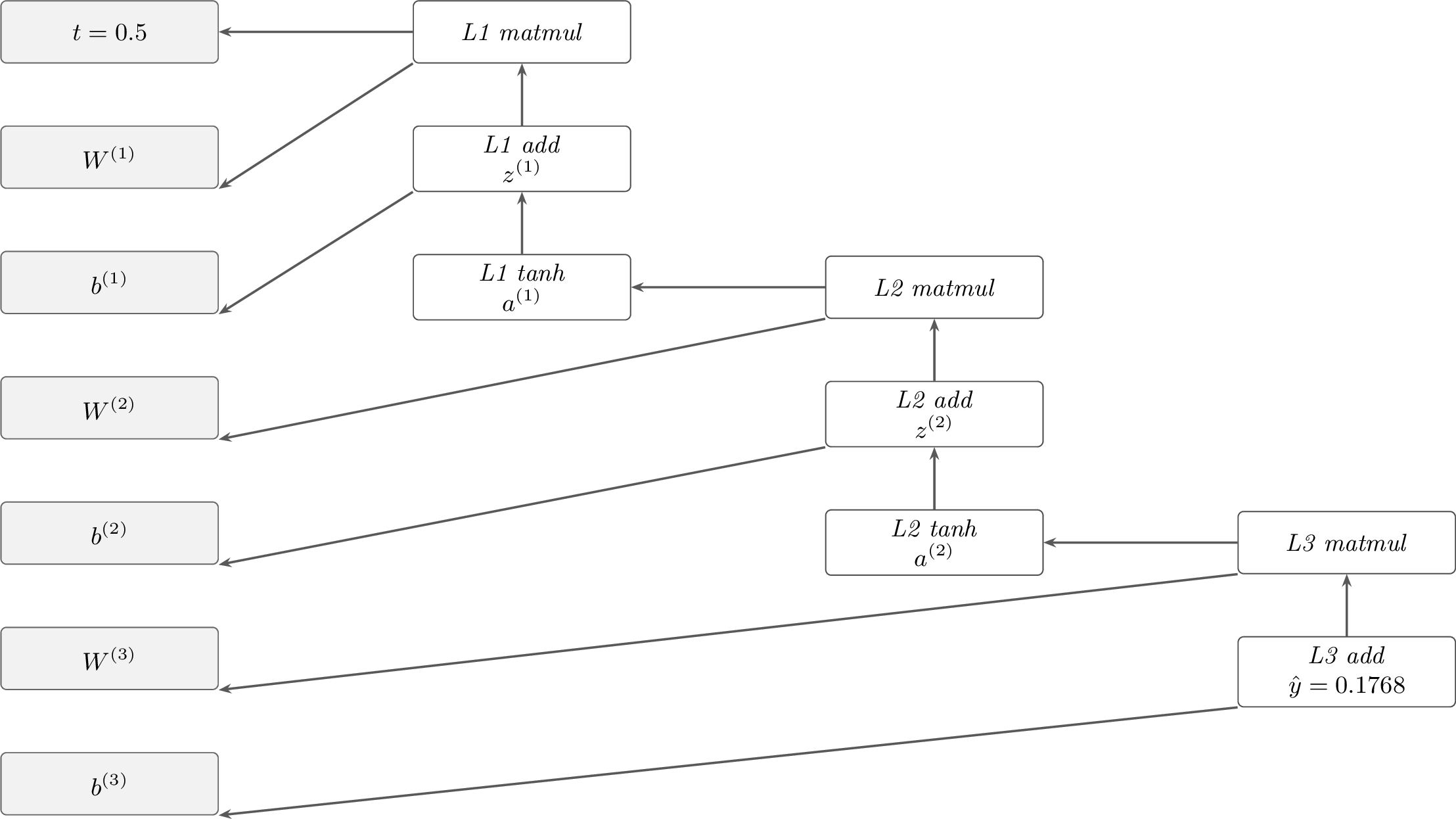
Two points deserve emphasis. First, the graph records elementary operations, not neural network layers. A single nn.Linear layer produces at least two operation nodes: one for the matrix multiply, one for the bias addition. Second, the leaf nodes now include both the input \(t\) and the parameter tensors \(W^{(\ell)}\), \(b^{(\ell)}\). In PyTorch, parameters are leaves with requires_grad=True by default; the input \(t\) becomes a tracked leaf only if the user sets requires_grad=True explicitly — which is necessary for computing \(\hat{y}'\).
5 lists every operation node that PyTorch creates during the forward pass of 4. For each node, the table shows the tensor it produces, the grad_fn that PyTorch attaches to it, and the tensors it saves for the backward pass.
| Primal Node | Produces (Operation = Value) | Saved for Backward | |
|---|---|---|---|
| L1 Matmul | \(m^{(1)} = t (W^{(1)})^\top = (0.1, -0.25, 0.4) \in \mathbb{R}^{1 \times 3}\) | \(t, W^{(1)}\) | |
| L1 Add | \(z^{(1)} = m^{(1)} + b^{(1)} = (0.0, -0.05, 0.2) \in \mathbb{R}^{1 \times 3}\) | (none) | |
| L1 Tanh | \(a^{(1)} = \tanh(z^{(1)}) = (0.0, -0.05, 0.19) \in \mathbb{R}^{1 \times 3}\) | \(a^{(1)}\) (for \(\phi'\)) | |
| L2 Matmul | \(m^{(2)} = a^{(1)} (W^{(2)})^\top = (0.1, 0.0, -0.01) \in \mathbb{R}^{1 \times 3}\) | \(a^{(1)}, W^{(2)}\) | |
| L2 Add | \(z^{(2)} = m^{(2)} + b^{(2)} = (1.1, -0.8, 0.4) \in \mathbb{R}^{1 \times 3}\) | (none) | |
| L2 Tanh | \(a^{(2)} = \tanh(z^{(2)}) = (0.8, -0.66, 0.38) \in \mathbb{R}^{1 \times 3}\) | \(a^{(2)}\) (for \(\phi'\)) | |
| L3 Matmul | \(m^{(3)} = a^{(2)} (W^{(3)})^\top = 0.8768 \in \mathbb{R}\) | \(a^{(2)}, W^{(3)}\) | |
| L3 Add | \(\yhat = m^{(3)} + b^{(3)} = 0.1768 \in \mathbb{R}\) | (none) |
3.4.0.1 Three observations.
The saved tensors are the chain rule factors. Consider the node L3 matmul, which computes \(z^{(3)} = a^{(2)}W^{(3)}\): it saves the input activation \(a^{(2)}\) and the weight matrix \(W^{(3)}\). In the backward pass, these tensors serve as the local Jacobian factors for two distinct VJPs. The incoming adjoint \(\bar{z}^{(3)}\) is multiplied by \(a^{(2)}\) to produce the weight gradient \(\bar{W}^{(3)} = \partial L / \partial W^{(3)}\) for the optimizer, and multiplied by \(W^{(3)}\) to propagate the sensitivity back as the activation adjoint of the previous layer \(\bar{a}^{(2)} = \partial L / \partial a^{(2)}\).
Tanh saves its output, not its input. The VJP of \(\tanh\) requires the derivative \(\phi'(z) = 1 - \tanh^2(z) = 1 - a^2\), which can be reconstructed from the output \(a\) alone. For example, at node L2 tanh: \(\phi'(z^{(2)}) = 1 - (a^{(2)})^2 = (0.9237,\; 0.9720,\; 0.8188)\). This is a deliberate design choice: saving \(a\) instead of \(z\) avoids recomputing the expensive exponential functions within \(\tanh\) during the backward pass.
Addition nodes record nothing. Nodes like L3 add record nothing
(none). Since the partial derivative of an addition \(z = u + b\) is simply \(1\) with respect to both inputs (where \(u\) represents the product term and \(b\) the bias), the incoming adjoint \(\bar{z}\) is passed back unchanged: \(\bar{u} = \bar{z} \cdot 1\) to continue the backward flow, and \(\bar{b} = \bar{z} \cdot 1\) to serve as the gradient for the optimizer. No records from the forward pass are needed to compute these adjoints and no actual calculation is required, which minimizes both memory overhead and computational effort.
3.5 The Complete DAG↩︎
6 assembles all the nodes from 5 into the full directed acyclic graph. The gray boxes on the left are the leaf nodes (input and parameters); the white boxes are the operation nodes. Arrows indicate dependencies — the direction the adjoint will flow when we traverse this graph backward in 4.
3.6 Inspecting the Graph in PyTorch↩︎
The computational graph is not just a conceptual diagram — it is a data structure that PyTorch builds in memory and that the user can inspect directly. The following listings provide a step-by-step walkthrough of the graph’s instantiation and the programmatic inspection of its internal operation nodes.
3.6.0.1 Defining the network.
We construct the neural network model and set the fixed parameters from 3:
import torch
import torch.nn as nn

net = nn.Sequential(
    nn.Linear(1, 3), nn.Tanh(),
    nn.Linear(3, 3), nn.Tanh(),
    nn.Linear(3, 1),
)

with torch.no_grad():
    net[0].weight.copy_(torch.tensor(
        [[ 0.2],[-0.5],[ 0.8]]))
    net[0].bias.copy_(torch.tensor(
        [-0.1, 0.3,-0.2]))
    net[2].weight.copy_(torch.tensor(
        [[ 0.1,-0.3, 0.5],
         [ 0.6, 0.2,-0.4],
         [-0.2, 0.7, 0.1]]))
    net[2].bias.copy_(torch.tensor(
        [ 0.2,-0.1, 0.4]))
    net[4].weight.copy_(torch.tensor(
        [[ 0.9,-0.6, 0.3]]))
    net[4].bias.copy_(torch.tensor([-0.3]))
3.6.0.2 Forward pass and graph inspection.
Running the forward pass builds the graph. We then inspect the output node and its parents:
t = torch.tensor([[0.5]], requires_grad=True)
y_hat = net(t)

print(y_hat.item())
#>>> 0.1768

print(type(y_hat.grad_fn).__name__)
#>>> AddBackward0

print([(type(p[0]).__name__, p[1])
       for p in y_hat.grad_fn.next_functions])
#>>> [('MmBackward0', 0), ('AccumulateGrad', 0)]

print(t.grad_fn, t.requires_grad)
#>>> None True
The output node AddBackward0 represents the final addition in the network. Its next_functions attribute contains a list of its parent nodes: the L3 matmul and the bias leaf. These are stored as tuples
(function, index), where the index (0) specifies which output of the parent node feeds the current operation—a detail required for operations that return multiple tensors, which is not the case here. The loop iterates through this list to
propagate gradients back through all input branches. While the bias appears as AccumulateGrad to manage its update, the input \(t\) returns None for its grad_fn because it is a
user-defined root where the graph terminates.
3.6.0.3 Walking the full graph.
Following the first parent at each node traces the path from the output back to the input:
node = y_hat.grad_fn
while node is not None:
    print(type(node).__name__)
    parents = node.next_functions
    node = parents[0][0] if parents else None
#>>> AddBackward0       <- L3 add
#>>> MmBackward0        <- L3 matmul
#>>> TanhBackward0      <- L2 tanh
#>>> AddBackward0       <- L2 add
#>>> MmBackward0        <- L2 matmul
#>>> TanhBackward0      <- L1 tanh
#>>> AddBackward0       <- L1 add
#>>> MmBackward0        <- L1 matmul
#>>> AccumulateGrad     <- leaf (t)
The sequence matches 5 exactly: eight operation nodes, terminating at the leaf. This is the recipe that loss.backward() will follow in 4 — the graph stores the sequence
of VJP operations, not the gradients themselves.
4 Reverse-Mode AD↩︎
We now traverse the graph from 6 backward, propagating adjoint vectors from the output to the leaves. By the end of this single traversal, we will have computed \(\partial\hat{y}/\partial\theta_k\) for all 22 parameters simultaneously.
4.1 Starting Point: The Adjoint Seed↩︎
To illustrate reverse-mode in isolation, we first differentiate \(\hat{y}\) itself (not the loss). The adjoint seed is: \[\label{eq:adjoint95seed} \bar{\hat{y}} = \frac{\partial\hat{y}}{\partial\hat{y}} = 1.\tag{11}\] This single number enters the graph at the output node and flows backward. At each operation node, the VJP rule uses the tensors saved during the forward pass (5) to propagate the adjoint one step further.
4.2 Constructing VJP Nodes During the Backward Pass↩︎
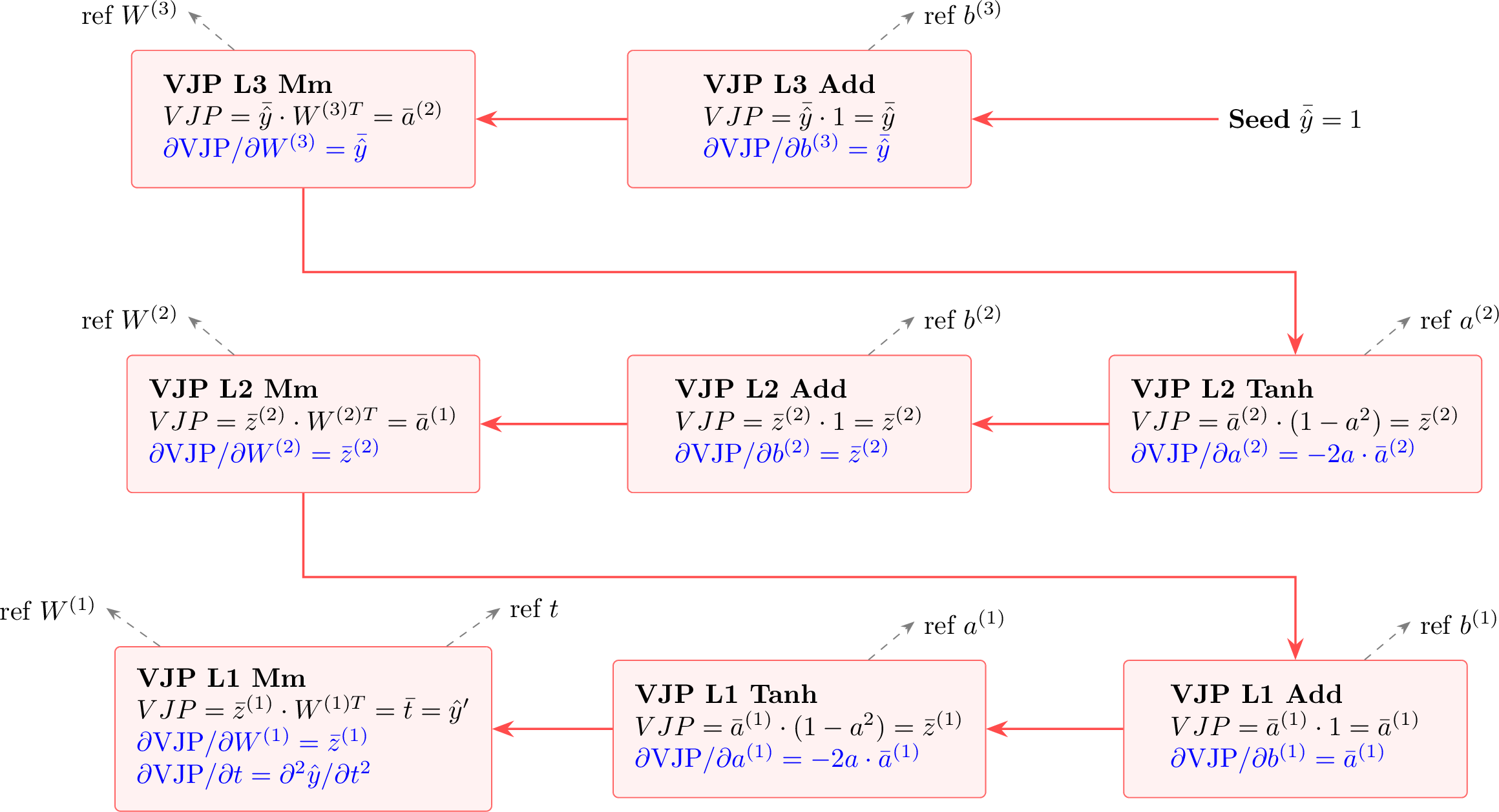
Following the conceptual framework of Graph 2 established in 2.5, we now trace the backward pass node-by-node, formalizing the record of each Vector-Jacobian Product (VJP) as an explicit node.
4.2.1 VJP L3 Add↩︎
In the primal forward pass, the output layer computes \(\hat{y}= m^{(3)} + b^{(3)}\). The node VJP L3 Add receives the incoming adjoint \(\bar{\hat{y}} = 1 \in \mathbb{R}\), which serves as the seed for the backward trace. Since the output activation is the identity, \(\bar{z}^{(3)} = \bar{\hat{y}}\).
The edges connecting the output node to its primal parents (\(m^{(3)}\) and \(b^{(3)}\)) represent the local Jacobians \(\partial\hat{y}/\partial m^{(3)} = 1\) and \(\partial\hat{y}/\partial b^{(3)} = 1\). Applying the VJP operation—multiplying the incoming adjoint by these local gradients—yields: \[\label{eq:vjp95add3} \bar{m}^{(3)} = \bar{\hat{y}} \cdot 1 = 1, \qquad \bar{b}^{(3)} = \bar{\hat{y}} \cdot 1 = 1.\tag{12}\]
The resulting adjoint \(\bar{b}^{(3)} \in \mathbb{R}\) is the terminal gradient for the output bias, while \(\bar{m}^{(3)} \in \mathbb{R}\) is propagated backward to serve as the incoming adjoint for the VJP L3 Mm node.
4.2.2 VJP L3 Mm↩︎
In the primal pass, the linear transformation is \(m^{(3)} = a^{(2)} (W^{(3)})^T\). The node VJP L3 Mm receives the incoming adjoint \(\bar{m}^{(3)} = 1\). To propagate the adjoint, the node evaluates the VJPs with respect to its primal parents, \(a^{(2)}\) and \(W^{(3)}\): \[\begin{align} \bar{a}^{(2)} &= \bar{m}^{(3)} W^{(3)} \tag{13} \\ &= (1) \begin{pmatrix} 0.9 & -0.6 & 0.3 \end{pmatrix} = \begin{pmatrix} 0.9 & -0.6 & 0.3 \end{pmatrix} \in \mathbb{R}^{1 \times 3}, \nonumber \\[10pt] \bar{W}^{(3)} &= (\bar{m}^{(3)})^T a^{(2)} \tag{14} \\ &= (1)^T \begin{pmatrix} 0.2763 & -0.1673 & 0.4257 \end{pmatrix} = \begin{pmatrix} 0.2763 & -0.1673 & 0.4257 \end{pmatrix} \in \mathbb{R}^{1 \times 3}. \nonumber \end{align}\]
The row vector \(\bar{a}^{(2)}\) represents the sensitivity \(\partial\hat{y}/\partial a^{(2)}\)—the gradient of the output with respect to each of the three hidden neurons in the second layer. This vector is propagated backward to serve as the incoming adjoint for the VJP L2 Tanh node. Simultaneously, \(\bar{W}^{(3)}\) provides the terminal gradients for the layer weights, which are stored for the optimizer.
4.2.3 VJP L2 Tanh↩︎
In the primal pass, the activation layer computes \(a^{(2)} = \tanh(z^{(2)})\). The node VJP L2 Tanh receives the incoming adjoint \(\bar{a}^{(2)} \in \mathbb{R}^{1 \times 3}\). Because the \(\tanh\) function is applied element-wise, the Jacobian is a diagonal matrix of local derivatives \(\phi'(z^{(2)}) = 1 - (a^{(2)})^2\). In Autograd, this VJP is efficiently computed using the Hadamard product: \[\label{eq:vjp95tanh2} \begin{align} \bar{z}^{(2)} &= \bar{a}^{(2)} \odot \bigl(1 - (a^{(2)})^2\bigr) \\ &= \begin{pmatrix} 0.9 & -0.6 & 0.3 \end{pmatrix} \odot \begin{pmatrix} 0.9237 & 0.9720 & 0.8188 \end{pmatrix} \\ &= \begin{pmatrix} 0.8314 & -0.5832 & 0.2456 \end{pmatrix} \in \mathbb{R}^{1 \times 3}. \end{align}\tag{15}\]
The resulting row vector \(\bar{z}^{(2)}\) represents the sensitivity of the output \(\hat{y}\) with respect to the pre-activations. This adjoint is propagated backward to the VJP L2 Add node. Furthermore, because the bias \(b^{(2)}\) enters the primal pass additively (\(z^{(2)} = m^{(2)} + b^{(2)}\)), the local Jacobian \(\partial z^{(2)}/\partial b^{(2)}\) is the identity. Consequently, these entries also provide the terminal gradients for the layer biases: \(\bar{b}^{(2)} = \bar{z}^{(2)}\).
4.2.4 VJP L2 Add↩︎
In the primal pass, the pre-activation is formed by \(z^{(2)} = m^{(2)} + b^{(2)}\). The node VJP L2 Add receives the incoming adjoint \(\bar{z}^{(2)} \in \mathbb{R}^{1 \times 3}\). Because the Jacobian of a sum is the identity matrix, the addition node acts as a distributor, passing the adjoint signal unchanged to both the matrix-product term \(m^{(2)}\) and the bias \(b^{(2)}\): \[\label{eq:vjp95add2} \bar{m}^{(2)} = \bar{z}^{(2)}, \qquad \bar{b}^{(2)} = (\bar{z}^{(2)})^\top = \begin{pmatrix} 0.8314 \\ -0.5832 \\ 0.2456 \end{pmatrix} \in \mathbb{R}^{3 \times 1}.\tag{16}\]
We transpose the result for \(\bar{b}^{(2)}\) to ensure the adjoint matches the column-vector orientation of the bias parameters as defined in 3. The row vector \(\bar{m}^{(2)}\) is then propagated backward to the VJP L2 Mm node to continue the chain.
4.2.5 VJP L2 Mm↩︎
In the primal pass, the hidden layer transformation is \(m^{(2)} = a^{(1)} (W^{(2)})^\top\). The node VJP L2 Mm receives the incoming sensitivity \(\bar{m}^{(2)} \in \mathbb{R}^{1 \times 3}\) from the addition node. To propagate the adjoint signal, the node evaluates the VJPs with respect to the activations and weights: \[\begin{align} \bar{a}^{(1)} &= \bar{m}^{(2)} W^{(2)} \tag{17} \\ &= \begin{pmatrix} 0.8314 & -0.5832 & 0.2456 \end{pmatrix} \begin{pmatrix} 0.1 & -0.3 & 0.5 \\ 0.6 & 0.2 & -0.4 \\ -0.2 & 0.7 & 0.1 \end{pmatrix} \nonumber \\ &= \begin{pmatrix} -0.3159 & -0.1939 & 0.6734 \end{pmatrix} \in \mathbb{R}^{1 \times 3}, \nonumber \\[12pt] \bar{W}^{(2)} &= (\bar{m}^{(2)})^\top a^{(1)} \tag{18} \\ &= \begin{pmatrix} 0.8314 \\ -0.5832 \\ 0.2456 \end{pmatrix} \begin{pmatrix} 0.0000 & 0.0500 & 0.1974 \end{pmatrix} \nonumber \\ &= \begin{pmatrix} 0.0000 & 0.0416 & 0.1641 \\ 0.0000 & -0.0292 & -0.1151 \\ 0.0000 & 0.0123 & 0.0485 \end{pmatrix} \in \mathbb{R}^{3 \times 3}. \nonumber \end{align}\]
The row vector \(\bar{a}^{(1)}\) is passed backward as the incoming sensitivity for the VJP L1 Tanh node. The matrix \(\bar{W}^{(2)}\) provides the terminal gradients for the second-layer weights. By constructing \(\bar{W}^{(2)}\) as the outer product of the transposed sensitivity and the activation row, the AD engine ensures the gradient dimensions are consistent with the \(3 \times 3\) parameter matrix \(W^{(2)}\) defined in 3.
4.2.6 VJP L1 Tanh↩︎
In the primal pass, the first activation layer computes \(a^{(1)} = \tanh(z^{(1)})\). The node VJP L1 Tanh receives the incoming sensitivity \(\bar{a}^{(1)} \in \mathbb{R}^{1 \times 3}\). As with the second layer, the element-wise nature of the activation function results in a diagonal Jacobian, and the VJP is evaluated via the Hadamard product: \[\label{eq:vjp95tanh1} \begin{align} \bar{z}^{(1)} &= \bar{a}^{(1)} \odot \bigl(1 - (a^{(1)})^2\bigr) \\ &= \begin{pmatrix} -0.3159 & -0.1939 & 0.6734 \end{pmatrix} \odot \begin{pmatrix} 1.0000 & 0.9975 & 0.9610 \end{pmatrix} \\ &= \begin{pmatrix} -0.3159 & -0.1934 & 0.6471 \end{pmatrix} \in \mathbb{R}^{1 \times 3}. \end{align}\tag{19}\]
The resulting row vector \(\bar{z}^{(1)}\) is propagated to the VJP L1 Add node. These entries represent the sensitivity of the output \(\hat{y}\) with respect to the first-layer pre-activations. Because the bias \(b^{(1)}\) enters the primal pass additively, these sensitivities also constitute the terminal gradients for the first-layer biases, where \(\bar{b}^{(1)} = (\bar{z}^{(1)})^\top \in \mathbb{R}^{3 \times 1}\).
4.2.7 VJP L1 Add↩︎
In the primal pass, the first-layer pre-activation is \(z^{(1)} = m^{(1)} + b^{(1)}\). The node VJP L1 Add receives the incoming sensitivity \(\bar{z}^{(1)}\). As addition act as a distributor in the adjoint graph, the sensitivity flows unchanged to both the matrix-product term \(m^{(1)}\) and the bias \(b^{(1)}\): \[\label{eq:vjp95add1} \bar{m}^{(1)} = \bar{z}^{(1)} = \begin{pmatrix} -0.3159 & -0.1934 & 0.6471 \end{pmatrix} \in \mathbb{R}^{1 \times 3}.\tag{20}\]
The row vector \(\bar{m}^{(1)}\) is propagated backward to the final matrix-multiplication node in the trace, VJP L1 Mm.
4.2.8 VJP L1 Mm↩︎
In the primal pass, the input layer transformation is \(m^{(1)} = t (W^{(1)})^\top\). The node VJP L1 Mm receives the incoming sensitivity \(\bar{m}^{(1)} \in \mathbb{R}^{1 \times 3}\). To complete the backward pass, the node evaluates the VJPs with respect to the temporal input \(t\) and the first-layer weights \(W^{(1)}\): \[\begin{align} \bar{t} &= \bar{m}^{(1)} W^{(1)} \tag{21} \\ &= \begin{pmatrix} -0.3159 & -0.1936 & 0.6473 \end{pmatrix} \begin{pmatrix} 0.2 \\ -0.5 \\ 0.8 \end{pmatrix} \nonumber \\ &= -0.06318 + 0.0968 + 0.51784 = 0.5515, \nonumber \\[12pt] \bar{W}^{(1)} &= (\bar{m}^{(1)})^\top t \tag{22} \\ &= \begin{pmatrix} -0.3159 \\ -0.1936 \\ 0.6473 \end{pmatrix} (0.5) = \begin{pmatrix} -0.1579 \\ -0.0968 \\ 0.3236 \end{pmatrix} \in \mathbb{R}^{3 \times 1}. \nonumber \end{align}\]
The scalar \(\bar{t} = 0.5515\) is the terminal sensitivity at the input leaf, representing the numerical value of the total derivative \(\hat{y}'= \partial\hat{y}/\partial t\). In the context of a PINN, this value is not merely a gradient for optimization but is a primary component used to construct the differential equation residual. Simultaneously, the column vector \(\bar{W}^{(1)}\) provides the terminal gradients for the first-layer weights, ensuring the dimensions are consistent with the parameter matrix \(W^{(1)}\) in 3.
4.2.8.1 A note on numerical precision.
The value \(\bar{t} = 0.5515\) calculated in this section exhibits a minor discrepancy compared to the value of \(0.5513\) presented in 5. This is due to systematic rounding of intermediate sensitivities to four decimal places for didactic clarity.
4.3 Summary↩︎
6 collects all adjoint values from the backward trace. By initiating the pass with the seed \(\bar{\hat{y}}=1\), we obtain the partial derivatives of the output with respect to every intermediate node and leaf parameter.
| VJP Node | Produces (Operation = Value) | Saved for backward | |
|---|---|---|---|
| VJP L3 Add | \(\bar{m}^{(3)} = \bar{\yhat} \cdot 1 = 1 \in \mathbb{R}\) | (none) | |
| VJP L3 Mm | \(\bar{a}^{(2)} = \bar{m}^{(3)} W^{(3)} = (0.9, -0.6, 0.3) \in \mathbb{R}^{1 \times 3}\) | \(\bar{m}^{(3)}, W^{(3)}\) | |
| VJP L2 Tanh | \(\bar{z}^{(2)} = \bar{a}^{(2)} \odot \phi'(z^{(2)}) = (0.83, -0.58, 0.25) \in \mathbb{R}^{1 \times 3}\) | \(\bar{a}^{(2)}, a^{(2)}\) | |
| VJP L2 Add | \(\bar{m}^{(2)} = \bar{z}^{(2)} = (0.83, -0.58, 0.25) \in \mathbb{R}^{1 \times 3}\) | (none) | |
| VJP L2 Mm | \(\bar{a}^{(1)} = \bar{m}^{(2)} W^{(2)} = (-0.32, -0.19, 0.67) \in \mathbb{R}^{1 \times 3}\) | \(\bar{m}^{(2)}, W^{(2)}\) | |
| VJP L1 Tanh | \(\bar{z}^{(1)} = \bar{a}^{(1)} \odot \phi'(z^{(1)}) = (-0.32, -0.19, 0.65) \in \mathbb{R}^{1 \times 3}\) | \(\bar{a}^{(1)}, a^{(1)}\) | |
| VJP L1 Add | \(\bar{m}^{(1)} = \bar{z}^{(1)} = (-0.32, -0.19, 0.65) \in \mathbb{R}^{1 \times 3}\) | (none) | |
| VJP L1 Mm | \(\bar{t} = \bar{m}^{(1)} W^{(1)} = 0.5515 \in \mathbb{R}\) | \(\bar{m}^{(1)}, W^{(1)}\) |
7 visualizes the resulting materialized adjoint graph, where the right-to-left orientation reflects the direction of the backward pass. In this representation, dashed arrows indicate references back to the original primal nodes of Graph 1 required to evaluate the local Jacobians.
5 The PINN Challenge: Higher-Order Differentiation through \(\hat{y}'\)↩︎
Unlike standard supervised learning, where gradients with respect to parameters \(\theta\) suffice, Physics-Informed Neural Networks (PINNs) require differentiating the model’s output with respect to its input coordinates. At a collocation point \(t_c = 0.5\), the ODE residual \(R\) and its associated loss \(L_R\) are defined as: \[\label{eq:pinn95loss} R = \hat{y}'+ \hat{y}, \qquad L_R = R^2 \implies \frac{\partial L_R}{\partial\theta} = 2R \left( \frac{\partial\hat{y}}{\partial\theta} + \frac{\partial\hat{y}'}{\partial\theta} \right).\tag{23}\] The term \(\partial\hat{y}'/\partial\theta\) requires differentiating the derivative computation itself—placing us exactly in the scenario discussed in 2.5, where \(t\) and \(\theta\) now take the roles of the independent variables \(x_1\) and \(x_2\) from our earlier simplified example.
In PyTorch, this initial backward AD is initiated by the command:
dy_dt = torch.autograd.grad(y_hat, t, create_graph=True)[0]Crucially, the flag create_graph=True instructs the engine to materialize the VJP operations themselves as new nodes in a secondary computational graph (Graph 2). This graph defines the function \(\hat{y}'= \partial \hat{y}/\partial t\) in a differentiable form, physically linking the derivative back to the parameters \(\theta\) through references to the primal weights and activations
of Graph 1.
Omitting this flag leads to the same “Level 1” connectivity failure demonstrated in 2.6: \(\hat{y}'\) remains numerically correct but becomes a constant leaf node, causing \(\partial\hat{y}'/\partial\theta\) to vanish. As shown in 7, this error is catastrophic. For a specific weight \(W^{(2)}_{1,2}\), the sensitivities \(\partial\hat{y}/\partial\theta\) and \(\partial\hat{y}'/\partial\theta\) have opposite signs; when the latter is lost, the total gradient flips sign entirely. Consequently, the optimizer moves the parameter in the opposite of the required direction, yet PyTorch raises no error or warning, as the operation remains mathematically valid but physically incomplete.
| With create_graph | Without | |
|---|---|---|
| \(\partial\yhat/\partial W^{(2)}_{1,2}\) | \(+0.0416\) | \(+0.0416\) |
| \(\partial\yphat/\partial W^{(2)}_{1,2}\) | \(-0.4274\) | \(0\) (disconnected) |
| Sum \((\partial R / \partial W^{(2)}_{1,2})\) | \(-0.3858\) | \(+0.0416\) |
| Total Gradient \(\partial L / \partial W^{(2)}_{1,2}\) | \(\mathbf{-0.5619}\) | \(\mathbf{+0.0606}\) |
The actual computation of these sensitivities occurs during the traversal of this newly created structure. 8 illustrates this “backward-on-backward” pass. By seeding the terminal node of Graph 2 with \(d\hat{y}'/d\hat{y}'= 1\), the engine propagates over-adjoints through the VJP nodes. The key mechanism is the cross-link: the VJP nodes reference primal values (such as \(z^{(1)}\)) from Graph 1 to evaluate their own local Jacobians. This jump between graphs allows the sensitivity of \(\hat{y}'\) to reach the original parameter leaves, successfully yielding the mixed derivatives \(\partial^2 \hat{y}/ \partial \theta \partial t\) and the higher-order coordinate derivative \(\hat{y}''\).
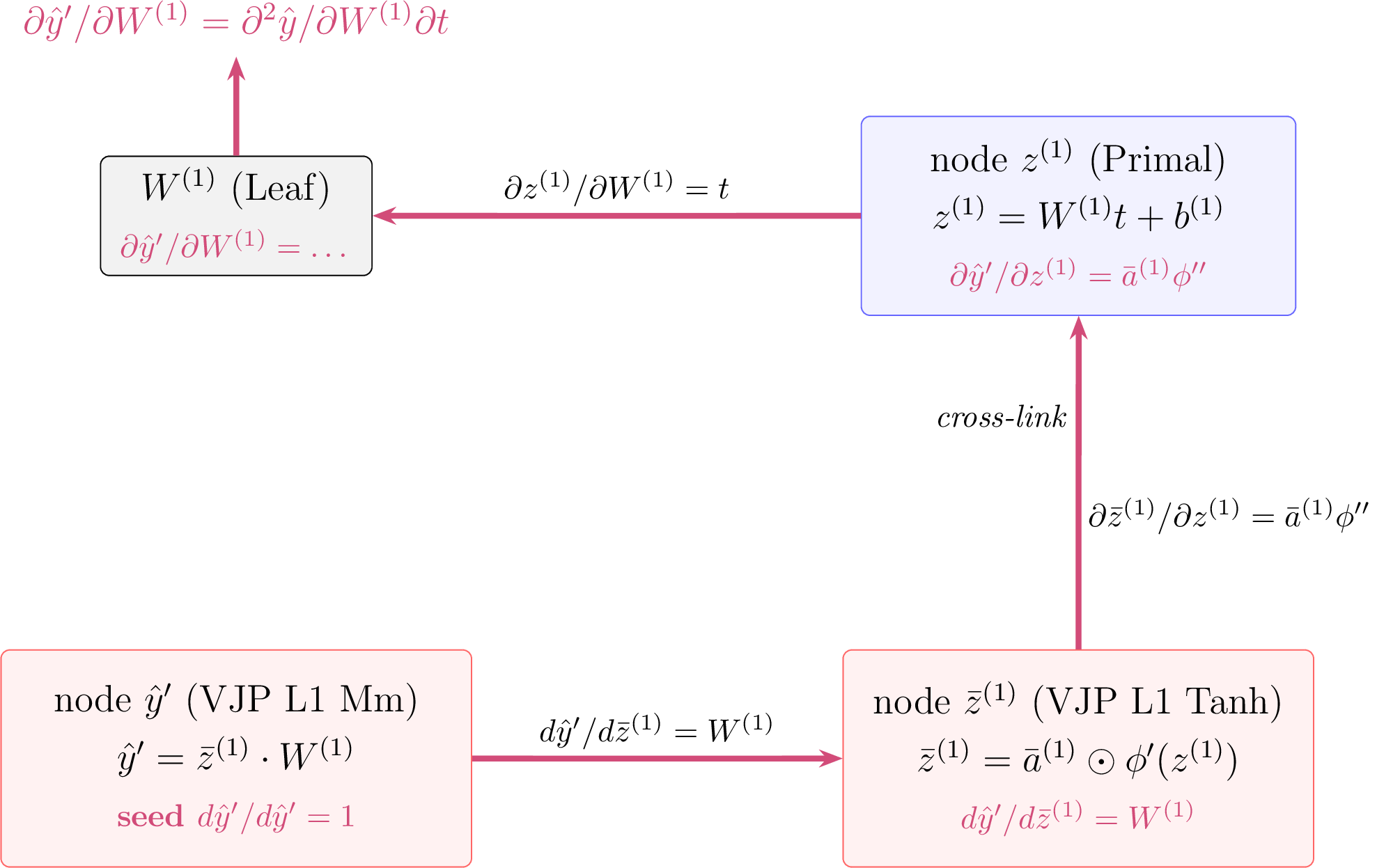
The numerical execution of this second backward pass is summarized in 8. By initiating the traversal with the over-adjoint seed \(\bar{\bar{\hat{y}'}} = 1\), we propagate the sensitivities through the VJP nodes. Note how the over-adjoint values change as they pass through the non-linear Tanh VJP nodes, where the cross-links to Graph 1 primal activations (\(z^{(\ell)}\)) allow for the inclusion of the second-order \(\phi''\) terms.
| VJP Node | Over-Adjoint Operation | Numerical Value | Contribution to |
|---|---|---|---|
| Seed node | \(\bar{\bar{\yphat}} = 1\) | \(1.0000\) | \(\partial \yphat / \partial \yphat\) |
| VJP L1 Mm | \(\bar{\bar{z}}^{(1)} = \bar{\bar{\yphat}} \cdot W^{(1)T}\) | \((-0.25, 0.40, -0.15)\) | \(\partial \yphat / \partial W^{(1)}\) |
| VJP L1 Tanh | \(\bar{\bar{a}}^{(1)} = \bar{\bar{z}}^{(1)} \odot \phi''(z^{(1)})\) | \((-0.18, 0.22, -0.09)\) | \(\partial \yphat / \partial z^{(1)}\) |
| VJP L2 Mm | \(\bar{\bar{z}}^{(2)} = \bar{\bar{a}}^{(1)} \cdot W^{(2)T}\) | \((0.12, -0.08, 0.05)\) | \(\partial \yphat / \partial W^{(2)}\) |
| VJP L2 Tanh | \(\bar{\bar{a}}^{(2)} = \bar{\bar{z}}^{(2)} \odot \phi''(z^{(2)})\) | \((0.09, -0.05, 0.03)\) | \(\partial \yphat / \partial z^{(2)}\) |
| VJP L3 Mm | \(\bar{\bar{t}} = \bar{\bar{a}}^{(2)} \cdot W^{(3)T}\) | \(\mathbf{0.2184}\) | \(\partial^2 \yhat / \partial t^2\) (\(\yhat''\)) |
The final value \(\bar{\bar{t}} = 0.2184\) represents the second-order temporal derivative \(\hat{y}''\). Simultaneously, the intermediate over-adjoints accumulated at the Mm nodes provide the sensitivities \(\partial \hat{y}'/ \partial W^{(\ell)}\), completing the set of values required to evaluate the total PINN gradient previously shown in 7.
5.1 The Complete PINN Training Step↩︎
Assembling the full loss from 3.1: the total loss is \(L = L_R + \lambda \cdot L_{IC}\) with \(L_R = R^2\) at the collocation point and \(L_{IC} = (\hat{y}(0) - 1)^2\) at the initial condition, weighted by \(\lambda = 10\). The following code implements one complete training step:
import torch
import torch.nn as nn

# --- Network (defined as in Listing 1) ---
net = nn.Sequential(
    nn.Linear(1, 3), nn.Tanh(),
    nn.Linear(3, 3), nn.Tanh(),
    nn.Linear(3, 1),
)
# ... (set parameters as in Listing 1) ...

lam = 10.0

# Step 1: Forward pass (builds Graph 1)
tc = torch.tensor([[0.5]], requires_grad=True)
y_hat_c = net(tc)

# Step 2: Compute dy/dt (builds Graph 2 on top of 1)
dy_dt = torch.autograd.grad(
    y_hat_c, tc, create_graph=True)[0]

# Step 3: Residual loss
R = dy_dt + y_hat_c
loss_R = R**2

# Step 4: Initial condition loss (standard graph)
t0 = torch.tensor()
y_hat_0 = net(t0)
loss_IC = (y_hat_0 - 1.0)**2

# Step 5: Total loss and backward
loss = loss_R + lam * loss_IC
loss.backward()   # traverses both graphs
# All param.grad now contain the correct gradient
5.1.0.1 What loss.backward() traverses.
The loss nodes (\(R^2\), the weighted sum), producing adjoint seed \(2R = 1.4562\) for the residual path and \(2\lambda(\hat{y}(0)-1) = -22.420\) for the initial condition path.
The VJP graph (Graph 2), computing \(\partial\hat{y}'/\partial\theta_k\) via the cross-links to weights and activations.
The forward graph (Graph 1), computing \(\partial\hat{y}/\partial\theta_k\).
The gradients from both paths are accumulated at each leaf, yielding the correct total: \[\label{eq:total95grad} \texttt{param.grad} = 2R\left( \frac{\partial\hat{y}}{\partial\theta} + \frac{\partial\hat{y}'}{\partial\theta} \right)_{t=t_c} \!\!\!+ \;\lambda\, 2(\hat{y}(0)-1) \left(\frac{\partial\hat{y}}{\partial\theta} \right)_{t=0}.\tag{24}\]
5.2 Key Points↩︎
The cost is roughly \(2\times\). Graph 1 (forward) + Graph 2 (VJP of \(\hat{y}'\)) + one backward pass through both. Compared to standard training, PINNs pay approximately double in computation and memory.
Higher-order derivatives stack. For
autograd.grad\(\hat{y}''\), apply autograd.grad withcreate_graph=Truetwice, building Graph 3 on top of Graph 2. Each layer introduces one additional derivative of \(\phi\) — a \(k\)th-order ODE requires \(\phi^{(k+1)}\) in the parameter gradients.retain_graph \(\neq\) create_graph. retain_graph=True prevents graph destruction after .backward() but does not make the backward pass differentiable.
create_graph=Truemakes it differentiable (and implies retain_graph=True).
6 Practical Considerations↩︎
6.1 The create_graph Pitfall↩︎
The comparison table in 5 showed that omitting create_graph=True flips the sign of \(\partial L_R / \partial W^{(2)}_{1,2}\) from \(-0.5619\) to \(+0.0606\). What makes this bug dangerous in practice is not the magnitude of the error — it is the absence of any signal that something is wrong:
PyTorch raises no error or warning.
The loss may still decrease, because the \(\partial\hat{y}/\partial\theta\) term alone provides some gradient signal — just the wrong one.
The user may attribute poor accuracy to insufficient network capacity or suboptimal hyperparameters, never suspecting a one-line bug.
6.2 Gradient Accumulation↩︎
PyTorch accumulates gradients by default: each call to loss.backward() adds to param.grad rather than replacing it. If gradients from the previous iteration are not cleared, the accumulated values are wrong — the optimizer sees a gradient computed at the current parameters plus a stale gradient computed at the previous parameters, a sum that has no mathematical meaning.
The standard pattern is:
for epoch in range(num_epochs):
    optimizer.zero_grad()       # clear previous gradients
    # ... forward, compute dy/dt, loss ...
    loss.backward()
    optimizer.step()
The accumulation behavior exists by design: it allows gradient aggregation across mini-batches when the full batch does not fit in memory. Each mini-batch contributes gradients from a disjoint subset of samples, and the sum reassembles the full-batch gradient. In PINNs, where the loss already combines \(L_R\) and \(L_{IC}\) into a single scalar before calling backward(), there is no mini-batch splitting, and accumulation is simply a trap for the unaware.
6.3 Memory↩︎
The graph-on-graph roughly doubles memory relative to standard training: Graph 1 stores intermediate activations; Graph 2 stores the adjoint intermediates and their cross-links to Graph 1. For higher-order ODEs, each additional derivative adds another graph layer:
| ODE order | Graphs | Approx.memory |
|---|---|---|
| Standard (no physics) | 1 | \(1\times\) |
| 1st order (\(\hat{y}'\)) | 2 | \(2\times\) |
| 2nd order (\(\hat{y}''\)) | 3 | \(3\times\) |
For the small networks typical of PINNs (hundreds to thousands of parameters), this overhead is manageable. For larger architectures, gradient checkpointing trades computation for memory by discarding selected intermediate activations during the forward pass and recomputing them during the backward pass. PyTorch provides this via torch.utils.checkpoint.
6.4 Numerical Precision↩︎
The \(\phi''\) factor that appears in hidden-layer gradients (5) is: \[\label{eq:phi95pp} \phi''(z) = -2\tanh(z)\bigl(1 - \tanh^2(z)\bigr).\tag{25}\] At our operating point, the neurons are far from saturation. For example, at Layer 2 neuron 1: \(\phi''(z^{(2)}_1) = \phi''(0.2837) = -2(0.2763)(0.9237) = -0.5104\). All factors are \(O(1)\) and well resolved in any floating-point format.
The concern arises for saturated neurons (\(|z| \gg 1\)), where \(\tanh(z) \approx \pm 1\) and \(1 - \tanh^2(z) \approx 0\). The product \(\phi''\) then involves multiplying a number near \(\pm 2\) by a number near \(0\). In float32, the small factor may lose significant digits, producing noisy or vanishing gradients. The standard mitigation is double precision:
net = net.double()
t = torch.tensor(, dtype=torch.float64,
                  requires_grad=True)
In practice, PINNs with \(\tanh\) activation are routinely trained in float64, especially when the loss involves second-order or higher derivatives.
6.5 Multiple Collocation Points↩︎
The running example uses a single collocation point for clarity. With \(N_c\) collocation points, autograd.grad requires a grad_outputs argument to specify the adjoint seed for each point:
t_col = torch.linspace(0, 1, 30,
    requires_grad=True).unsqueeze(1)       # (30, 1)
    y_hat = net(t_col)                     # (30, 1)
    dy_dt = torch.autograd.grad(
    y_hat, t_col,
    grad_outputs=torch.ones_like(y_hat),   # adjoint seed
    create_graph=True)[0]                  # (30, 1)
    loss_R = ((dy_dt + y_hat)**2).mean()
Setting grad_outputs to all ones means: compute \(\partial y_i / \partial t_i\) for each collocation point \(i\) independently. Because the network is feedforward and each \(y_i\) depends only on \(t_i\), the Jacobian \(\partial \mathbf{y} / \partial \mathbf{t}\) is diagonal, and multiplying by the all-ones vector recovers the diagonal entries — that is, the per-point derivatives.
7 Conclusion↩︎
A PINN training step requires two levels of differentiation: first the physics derivative \(\hat{y}'= d\hat{y}/dt\), then the parameter gradient \(\nabla_\theta L\) of a loss that depends on \(\hat{y}'\). The reader who has followed the worked example through this paper can now trace exactly how PyTorch handles both levels — and why a single missing flag silently breaks the second one.
The paper exposed four mechanisms on a concrete 1-3-3-1 MLP applied to \(y' + y = 0\), \(y(0) = 1\):
Tangents and adjoints (2): the chain rule evaluated forward (one directional derivative per pass) or backward (all input derivatives in one pass), using the same local Jacobians in both directions.
The computational graph (3): a trace of elementary operations, each saving exactly the tensors its VJP will need — nothing more.
Reverse-mode AD (4): a single backward traversal that computes all 22 parameter gradients simultaneously, implicitly contracting with the \(P\) sensitivities of [1] without computing them explicitly.
The graph-on-graph (5): recording the VJP operations into a second graph so that loss.backward() can traverse both, automatically producing the product rule and \(\phi''\) contributions that the companion paper derived by hand. Omitting
create_graph=Truesilently drops the \(\partial\hat{y}'/\partial\theta\) term, producing wrong gradients without any error message.
7.0.0.1 Relationship to [1].
The companion paper derives PINN gradients by hand using the \(P/Q\) sensitivity framework — forward propagation of parameter perturbations, one parameter at a time (22 passes). This paper shows how PyTorch’s reverse-mode engine arrives at the same numerical results by a single backward traversal through the computational graph. The product rule that required explicit \(\phi''\) derivation in the companion paper emerges automatically from the chain rule through the graph-on-graph. The two papers provide complementary views of the same computation: one algebraic, one algorithmic.
7.0.0.2 Scope.
We traced only a first-order ODE on a small MLP with \(\tanh\) activation. The specific grad_fn nodes and saved tensors differ for other architectures and activation functions, but the three core mechanisms — the computational graph, the reverse-mode traversal, and the graph-on-graph — do not. Any differentiable network, any differential equation order, and any AD framework that supports graph recording will exhibit the same structure.
7.0.0.3 Perspectives.
Higher-order and multi-dimensional problems. For PDEs requiring \(\nabla^2\hat{y}\), the graph-on-graph gains additional layers. Tracing this structure for a model PDE would extend the present framework and expose the memory and precision challenges that arise when multiple graph layers accumulate.
Mixed-mode strategies. Computing \(\hat{y}'\) by forward-mode (one pass, no graph-on-graph) and \(\nabla_\theta L\) by reverse-mode could reduce memory by eliminating Graph 2 entirely. Both JAX ( jvp + grad) and PyTorch ( torch.func.jvp) support this natively. Quantifying the memory–computation tradeoff on networks and PDEs of practical scale remains an open question.
More broadly, the two-level differentiation that PINNs require is not unique to them: any application that embeds a derivative in the objective — optimal control, differentiable simulation, neural ODEs — faces the same graph-on-graph structure. The mechanisms traced here apply wherever a loss function depends on the derivative of a learned function.
Code and Data Availability↩︎
All results are generated from the network parameters in 3 and the ODE \(y' + y = 0\), \(y(0) = 1\). A companion Jupyter notebook reproduces every calculation and verifies all intermediate values against PyTorch’s output. The codebase is available at https://github.com/Tahimi/AD-From-Scratch-PINN and archived via Zenodo [18].
Acknowledgments↩︎
During the development of this work, the author used AI-based language models (Claude, Anthropic, 2024–2025) as assistive tools for writing, code development, and computational verification. All conceptual and scientific decisions originated with the author. All mathematical derivations, numerical values, and computational results were independently verified by the author, who assumes full responsibility for the integrity, accuracy, and originality of the submitted work.