Watermark Forensics for Generative Models: An Information-Theoretic Perspective
July 14, 2026
Watermark Forensics for Generative Models
An Information-Theoretic Perspective
| Xiaoyu Li\(^{1}\) | Zheng Gao\(^{1}\) | Xiaoyan Feng\(^{2}\) |
| Jiaojiao Jiang\(^{1}\) | Yulei Sui\(^{1}\) | Jiankun Hu\(^{1}\) |
\(^{1}\)University of New South Wales \(^{2}\)Griffith University
{xiaoyu.li2, zheng.gao1, jiaojiao.jiang, yulei.sui}unsw.edu.au?
xiaoyan.feng@griffithuni.edu.auj.hu@adfa.edu.au
2026-07-16
Abstract. A watermark in a generative model’s output is normally asked only whether a text is machine-made. The same mark can do more: attribute it to the user who produced it, extract a hidden payload, or localize the part that survives editing. These form a forensic ladder, and we ask what each rung costs in the sample length \(n\).
A single object organizes the answers. Let \(S\) be the secret the mark carries (a user’s identity, a payload), and let the information profile \(\nu(t)=I(S;X_t\mid X_{<t})\) measure how much the \(t\)-th token reveals about \(S\) given the earlier ones. Its total pays for attribution and extraction; how it is spread across the text pays for localization; and detection alone is paid for not by information but by presence, the distance from the marked to the unmarked distribution. The two quality models in the literature, a mark subtle on every token and one that stamps a few tokens loudly, are then incomparable ways of capping this one profile.
Our main theorem settles the ladder’s entropy column. For schemes that leave the model’s output distribution statistically intact, attributing a text to one of \(N\) users costs \(\Theta(\log N / h)\) tokens over every stationary-ergodic source of entropy rate \(h\), sharp to a \((1+o(1))\) factor; to our knowledge the first tight entropy-rate law for multi-user attribution (via exact alignment; the edit-robust case is open). A warning: the natural collision-counting argument overcharges without bound, and only a decoder that scores each candidate by its own realized surprisal, not against the others, attains the rate while almost never implicating an innocent user. A matching converse makes the law two-sided, and the same accounting prices extraction of an \(\ell\)-bit payload at \(\Theta(\ell/h)\). Two gaps are real rather than modeling artifacts: a window \(\Theta(\log N)\) tokens wide in which a text is provably machine-made yet unattributable, and an uncertainty principle trading a mark’s footprint against its localization resolution. Since emerging regulation presumes an extractable mark, these are limits it inherits rather than escapes.
Across three language models (GPT-2, Pythia-410M, Qwen2.5) under deployed watermarks, the predicted constants appear: the collision analysis overcharges by about \(1.6\times\), and detection saturates its \(\Theta(\log N)\) window before attribution begins.
Figure 1: 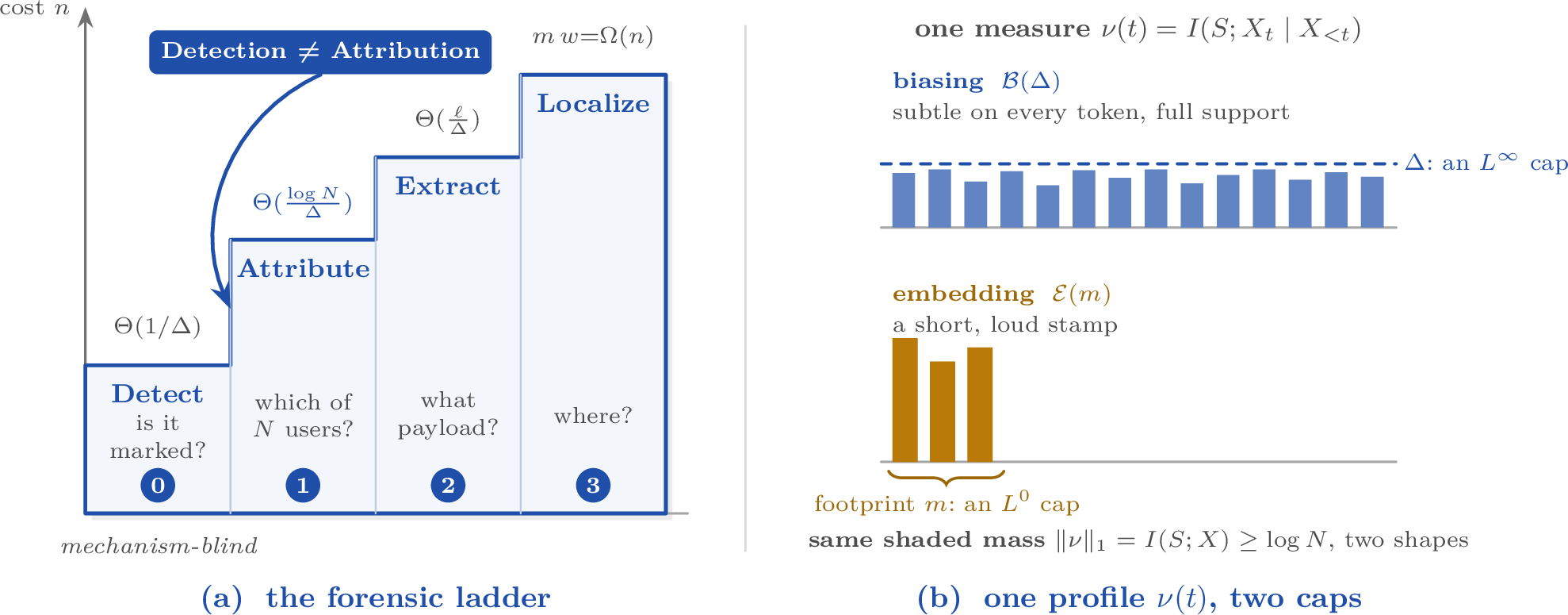 .
.
1 Introduction↩︎
Consider two deployed watermarks for generative models. Tree-Ring [1] embeds a ring pattern into the Fourier spectrum of a diffusion model’s initial noise; to test an image one inverts the generation and matches the ring. The green-list of [2] colours half the vocabulary green at each decoding step and tilts the next token toward it; to test a passage one counts green tokens. Tuned to the same detection ROC, the two are interchangeable for the question is this AI-generated. Now ask a second question. Given the marked image, can one point to where the mark lives? Yes: invert to the noise and read off the ring. Given the marked text, can one point to which tokens are the mark? Not in any strict sense; every token is plausible under the natural distribution, and the mark exists only in the statistical aggregate of the whole passage. In the second case the watermark is a property of the carrier, not an object inside it, and asking which tokens are the mark is a category error, much as one cannot ask which molecules of a warm gas carry its temperature. The distinction has direct consequences for attribution, extraction, and regulation, and the literature treats it only case by case.
This paper makes that informal gap quantitative. We treat the forensic uses of a watermark as a ladder of four statistical problems on a length-\(n\) carrier: Level 0 detection (machine-generated or not), Level 1 attribution (which of \(N\) users produced it), Level 2 extraction (recover an \(\ell\)-bit payload), and Level 3 localization (which sub-region carries the mark). We ask for the sample complexity of each. The detection rung is by now well understood: under a per-token distortion budget \(\Delta\) (each marked conditional within KL \(\Delta\) of the natural one), detection costs \(\Theta(1/\Delta)\) tokens, with sharp constants [3]–[5]. We import this rung and never reprove it. Our question is what happens above it, and whether the embedding-versus-biasing distinction that separates our two examples is a real boundary or a matter of taste.
1.0.0.1 One object.
It is a real boundary, and one measure draws it. Every forensic question asks how much of the secret \(S\) a decoder can recover from the carrier \(X\); by data processing this is at most the mutual information \(I(S;X)\), the number of nats that observing \(X\) reveals about \(S\) (for attribution and distortion-free extraction, conditioned on the decoder’s public key registry; 2, and a primer on the information-theoretic notions is in 9). The chain rule resolves it position by position, \(I(S;X)=\sum_t I(S;X_t\mid X_{<t})\), each summand the information about \(S\) that the \(t\)-th token adds given its past. This is the information profile of the scheme’s forensic payload \(S\), \[\nu(t)\;:=\;I(S;X_t\mid X_{<t}),\qquad t=1,\dots,n.\] Attribution and extraction are recovery questions, how much of \(S\), so each is governed by the total mass \(\norm{\nu}_1=I(S;X)\); localization asks not how much but where, so it reads the shape \(\mathop{\mathrm{supp}}\nu\), the footprint of 1. Detection is the exception: the imported baseline asks only whether the mark is present, priced by how far the marked law sits from natural and not by the mass — a scheme can make \(S\) recoverable yet be undetectable without the key. Our two opening examples are the extremal profiles ([fig:hero]): the green-list spreads its mass \(\Delta\)-thin over every position, while Tree-Ring concentrates it on a vanishing set of transform coordinates. The profile is written once, at generation time: by data processing, no reading of the carrier can recover more about \(S\) than the sampler put in, so what any decoder can ever learn is fixed by the \(\nu\) the scheme writes. This is the paper’s one idea: the forensic power of a watermark is set by the information it makes recoverable, position by position — the profile — and not by the mechanics of how the mark is embedded. The literature asks four questions of a watermark and treats them as four problems; detection is the mechanism-blind baseline, and the three rungs above it are readings of \(\nu\). Everything below is a statement about functionals of it. The profile earns its keep as the object that unifies the ladder above detection — attribution, extraction, and localization, together with the two quality models, become functionals of one measure — more than as a proof device: the scalar mass \(\norm{\nu}_1\) already separates attribution and extraction, while the per-position shape does load-bearing work only in the mechanism dichotomy ([thm:dichotomy]) and in localization ([thm:crop]). We are explicit throughout about which is which.
1.0.0.2 Contributions.
The contribution is the object; each result below is a way of reading it.
One measure, two norms ([prop:profile]). The chain rule gives the exact identity \(\norm{\nu}_1=I(S;X)=\Phi(n)\), the quantity the forensic-recovery budget caps. The two quality models of the literature are then norm caps on \(\nu\): the distributional model \(\mathcal{B}(\Delta)\) caps it in \(L^\infty\) (\(\nu(t)\le\Delta\) at every position, via the golden formula), and the footprint model \(\mathcal{E}(m)\) caps it in \(L^0\) (\(\nu\) supported on at most \(m\) positions, by conditional screening). We organize what were two incomparable quality models and a separately stated footprint axis as one object read two ways; the incomparability becomes definitional, two norms on one measure. Only the mass is invariant to the choice of dictionary and ordering; the caps, like sparsity, are relative to a fixed basis. Crop-robustness is the one property not of \(\nu\) alone: it additionally needs an edit coupling on the carrier footprint.
The entropy column closes ([thm:entropyclose]). For statistically distortion-free schemes with i.i.d.per-user keys (the decoder knows \(p_{\mathrm{nat}}\) and the deployed key set), attribution among \(N\) users costs \[n_{\mathrm{att}}\;=\;\Theta\Big(\frac{\log N}{h}\Big), \qquad\text{and}\qquad n_{\mathrm{att}}\;=\;(1+o(1))\,\frac{\log N}{h}\] as the per-innocent false-positive level \(\delta\to0\) with \(\log(1/\delta)=o(\log N)\) (the \(\log(1/\delta)\) term is then lower order), for every stationary-ergodic source of entropy rate \(h>0\); the Shannon–McMillan–Breiman theorem is the only source hypothesis. To our knowledge this is the first tight \(h\)-rate for multi-user attribution. Achievability is a surprisal-threshold decoder, and its threshold is forced, not tuned: an innocent key matches the observed text only with probability \(p_{\mathrm{nat}}(X)=e^{-\imath(X)}\), where \(\imath(X)=-\log p_{\mathrm{nat}}(X)\) is the realized surprisal, so to implicate no innocent above \(\delta/N\) the decoder must answer only when \(\imath(X)>\tau=\log(N/\delta)\) (then \(p_{\mathrm{nat}}(X)<\delta/N\)); completeness only asks that the true text, being \(p_{\mathrm{nat}}\)-typical, clear that same bar, which it does once \(n\ge\tau/h\). The obvious decoder instead reports any consistent key; bounding its error means counting the innocents consistent by chance, \((N-1)e^{-nr_2}\), and waiting for that list to clear at \(\log N/r_2\), the Rényi-2 collision rate. But the forensic question is not list size; it is naming one user with a guarantee, governed by the Shannon rate \(h\). Since \(r_2\le h\), and can be far smaller, the consistency count overcharges by the unbounded factor \(h/r_2\) (8). That guarantee is exact and non-asymptotic, and for the deterministic witness scheme pointwise, which is the form a forensic guarantee has to take: no innocent user is implicated except with probability \(\delta/N\) — at every length, for every source, for every realized set of innocent keys. The matching converse is Fano plus a mixture-entropy bound on the i.i.d.key draw. Extraction is the same theorem at \(N=2^\ell\), giving \(\Theta(\ell/h)\) ([cor:extraction-h]). The entropy column of the ladder, previously a converse-only ledger, is thereby two-sided.
The rest of the ladder, as readings of \(\nu\) ([thm:budget] [thm:separation] [thm:dichotomy] [thm:crop] [prop:region]). The mass and the shape of one measure, read five more ways. The forensic-recovery budget \(\Phi(n)=\norm{\nu}_1\le n\Delta\), respectively \(\le n\,h_n\) (\(h_n:=H(p_{\mathrm{nat}}^{(n)})/n\downarrow h\), the entropy rate). The co-located window: a length at which a biasing watermark is detectable with error \(\to0\) yet every attribution rule errs with probability \(\to1\), within a single scheme. The dichotomy at the extremal profiles: \(\mathcal{B}(\Delta)\) couples, \(n_{\mathrm{att}}=\Omega(\log N/\Delta)\) (tight for regular mixing sources), while \(\mathcal{E}(m)\) decouples, \(n_{\mathrm{att}}=\Theta(\log N/\log q)\), \(\Delta\)-free; a localization map enables the cheaper model but does not decide it ([cor:bridge]). The footprint–resolution uncertainty \(m\cdot w=\Omega(n)\): fine-resolution crop-robustness forces full support. And the rate region: attribution and extraction split one mass, \(R_{\mathrm{att}}+R_{\mathrm{ext}}\le(1+o(1))\,n\Delta\), order-tight.
1.0.0.3 What is imported and what is ours.
The Level-0 detection rate and the fidelity–detectability frontier are imported [3]–[5], as is the distortion-free detection rate [6]. The attribution converse in the \(\mathcal{B}(\Delta)\) column is the single-user Fano specialization of the distortion-constrained fingerprinting converse of [7], [8]; we claim no novelty for it. The false-positive mechanism behind [thm:entropyclose] is the folklore likelihood-ratio Markov bound (a one-line change of measure); we claim its use here, not the inequality. Ours are: the profile as the organizing object and the norm-cap reading of the quality models; the closed entropy column, that is, the decoder, its exact false-positive side, and tightness at full stationary-ergodic generality; the co-located window; the footprint–resolution uncertainty; the rate region; and the taxonomy. We flag plainly that the entropy-column witness decodes by exact alignment and is not edit-robust; edit-robust \(\Delta\)-free attribution remains open. The closest prior work proves complementary things: [9] construct multi-user watermarks where detection is cheap and tracing is expensive, with a cryptographic counting argument but no tight information-theoretic rate in \(h\); [10] argue empirically that detection and attribution coincide under a strict threshold; the SoK of [11] taxonomizes schemes on a security axis, with no sample-complexity content; concurrent work [12] studies the scalar \(I(S;X)\) without the positional decomposition on which our questions turn. We position against each in 5.
1.0.0.4 Why these questions.
Watermarking is becoming provenance infrastructure: the mechanism by which a world filling with synthetic content is supposed to answer who made this. The four rungs of the ladder are the operational content of that hope, and they are not one capability but four, with four prices. What theory can contribute is the price list: which questions are priced by the population (attribution: a \(\log N\) toll in the appropriate currency), which are not (detection), and which are structurally unavailable (fine crop-robust localization for any small-footprint mark, [thm:crop]). Regulation makes the list concrete. Watermark statutes tacitly assume the embedding ontology, asking for marks “in a machine-readable format” and the like: language that presumes an extractable object. Our dichotomy prices that presumption: a biasing watermark cannot meet an attribution or localization mandate at any fidelity without a sample cost that diverges as the mark is made stealthier, and the closed entropy column gives an attribution mandate its price when the mark is distortion-free, \(\Theta((\log N+\log(1/\delta))/h)\) tokens with a per-innocent false-positive guarantee of \(\delta/N\). A statute can mandate a capability; it cannot repeal an inequality. We return to this in 6.
1.0.0.5 Organization.
2 sets the model, the quality assumptions, and the information profile ([prop:profile]). 3 states the results: the forensic-recovery budget, the closed entropy column ([thm:entropyclose]), the co-located window, the dichotomy, the uncertainty bound, and the rate region, with a numerical illustration and, on three watermarked language models (GPT-2, Pythia, Qwen2.5), a measurement of the operative constants (3.7). 4 reads twenty deployed schemes through the profile. 5 positions the paper against prior and concurrent work, 6 draws consequences and states the open problems, and 7 concludes. Proofs are in 10, which also contains the imported-results glossary (10.1), the scheme-by-scheme fit of the deployed watermarks (11), and a broader survey of adjacent work (12).
2 Model: the forensic ladder↩︎
The model has three ingredients: a carrier, the laws that generate it, and a keyed family that secretly selects among those laws; every forensic task is a question about the selection.
2.0.0.1 Carrier, model, keys.
Tokens are drawn from an alphabet \(\Sigma\) of size \(q:=|\Sigma|\); a carrier is a sequence \(X\in\mathcal{X}:=\Sigma^n\). An unmarked model induces the natural law \(p_{\mathrm{nat}}\) on \(\mathcal{X}\). A keyed watermarking scheme draws a secret key \(K\sim\mu\) from a key space \(\mathcal{K}\) and generates \(X\sim p_{\mathrm{wm}}^{(K)}\); write \(\bar p:=\mathbb{E}_K\,p_{\mathrm{wm}}^{(K)}\) for the key-averaged output law. The secret \(S\) (a user identity in \([N]\), an \(\ell\)-bit payload, or both) determines the key, \(K=K(S)\), so \(S\to K\to X\) is a Markov chain. The primary object throughout is the family of per-secret kernels \(p_{\mathrm{wm}}(\cdot\mid s,x_{<t})\) (the conditional next-token law under secret \(s\) given the prefix \(x_{<t}\)) from which key-averaged quantities are derived, never the reverse. Decoders are informed: an attribution decoder knows \(p_{\mathrm{nat}}\) and the key registry \(\kappa:=\{k_1,\dots,k_N\}\), and false-positive statements are averaged over the i.i.d.draw of those keys. Recoverable information is measured against this side information: throughout, the per-secret quantities — the kernels \(p_{\mathrm{wm}}(\cdot\mid S,x_{<t})\), the information profile \(\nu\), the distortion profile \(\bar d\), and the budget \(\Phi\) — are read conditionally on the registry \(\kappa\), written \(I(S;X)\), \(\bar d(t)\), and so on for brevity. Given \(\kappa\) the secret determines its key, \(K=k_S\), so each per-secret object is the realized per-key one and every average over \(S\) ranges over the enrolled keys. This conditioning is vacuous for a fixed registry (a single enrolled key, detection, or deterministic extraction). It matters for any randomized registry with exchangeable keys — bounded schemes included, since marginally over the key draw the carrier is independent of the secret — and is sharpest for the distortion-free witness of [thm:entropyclose], whose output is exactly \(p_{\mathrm{nat}}\): there the unconditional \(I(S;X)=0\) while the registry-conditional budget is positive, and it is that conditional quantity the converse bounds by \(nh_n\). All logarithms are natural unless a base is shown; \(\mathop{\mathrm{KL}}\!\left(\cdot \,\|\, \cdot\right)\) is relative entropy and \(I(\cdot;\cdot)\) mutual information, both in nats.
2.0.0.2 Quality as a budget.
Fidelity to the base model is what makes a watermark usable, and it is what constrains forensic power. We consider the two quality models that occur in practice, both stated on the per-secret kernels.
Write \(\bar d(t):=\mathbb{E}_{X_{<t}}\mathbb{E}_S\,\mathop{\mathrm{KL}}\!\left(p_{\mathrm{wm}}(\cdot\mid S,X_{<t}) \,\|\, p_{\mathrm{nat}}(\cdot\mid X_{<t})\right)\) for the per-secret distortion profile (expectations under the joint marked law), so by the chain rule \(\sum_{t=1}^n\bar d(t)=\mathbb{E}_S\,\mathop{\mathrm{KL}}\!\left(p_{\mathrm{wm}}(\cdot\mid S) \,\|\, p_{\mathrm{nat}}\right)\), and \(T:=\{t:p_{\mathrm{wm}}(\cdot\mid s,x_{<t})\ne p_{\mathrm{nat}}(\cdot\mid x_{<t})\text{ for some }s,x_{<t}\}\) for the per-secret footprint, the set of marked positions. A natural alternative is the key-averaged marginal profile \(\delta_{\mathrm{marg}}(t):=\mathbb{E}_{X_{<t}}\,\mathop{\mathrm{KL}}\!\left(\mathbb{E}_S\,p_{\mathrm{wm}}(\cdot\mid S,X_{<t}) \,\|\, p_{\mathrm{nat}}(\cdot\mid X_{<t})\right)\); joint convexity of relative entropy gives the bridge \(\delta_{\mathrm{marg}}(t)\le\bar d(t)\), and the inequality is strict in general (10.8). We retire the marginal profile because it cannot see information hidden in correlations across positions: the two-token parity scheme (10.8) has zero marginal distortion at every position, yet a decoder reads one full bit from it (\(\nu(2)=\log2\) below). Every cap below is therefore stated on the per-secret kernels.
Assumption 1 (Bounded-distortion quality; the class \(\mathcal{B}(\Delta)\)). There is a per-token budget \(\Delta\ge0\), imposed in one of two forms. Sup-form: \(\mathop{\mathrm{KL}}\!\left(p_{\mathrm{wm}}(\cdot\mid s,x_{<t}) \,\|\, p_{\mathrm{nat}}(\cdot\mid x_{<t})\right)\le\Delta\) for every secret \(s\), prefix \(x_{<t}\), and position \(t\). Avg-form: \(\max_t\bar d(t)\le\Delta\). The sup-form implies the avg-form, and we tag each claim with the form it needs: every converse below needs only the avg-form, while the exponential-tilting achievability witness satisfies the sup-form. By the chain rule the global divergence inherits the cap: \(\mathop{\mathrm{KL}}\!\left(p_{\mathrm{wm}}^{(k)} \,\|\, p_{\mathrm{nat}}\right)\le n\Delta\) for every key \(k\) under the sup-form, and \(\mathbb{E}_S\,\mathop{\mathrm{KL}}\!\left(p_{\mathrm{wm}}(\cdot\mid S) \,\|\, p_{\mathrm{nat}}\right)=\sum_t\bar d(t)\le n\Delta\) under the avg-form. Each token stays \(\Delta\)-close to natural on average; the mark is delocalized.
Assumption 2 (Distortion-free quality). The mixture is undetectable without the key, at one of two levels. Sequence level: \(\bar p=p_{\mathrm{nat}}\) (statistically) or \(\bar p\approx p_{\mathrm{nat}}\) up to a negligible distinguishing advantage (computationally) — the operational statement: no key-less observer detects the mark. Kernel level: \(\mathbb{E}_K\,p_{\mathrm{wm}}(\cdot\mid K,x_{<t})=p_{\mathrm{nat}}(\cdot\mid x_{<t})\) for every prefix \(x_{<t}\) — the structural statement, satisfied by the exact-sampler family (inverse-CDF / exponential-minimum sampling; [13]; 4), and implying the sequence level whenever the key coordinates consumed at distinct positions are position-independent. The per-key divergence \(\mathop{\mathrm{KL}}\!\left(p_{\mathrm{wm}}^{(k)} \,\|\, p_{\mathrm{nat}}\right)\) is unconstrained; the binding resource is the generation entropy \(h_n:=H(p_{\mathrm{nat}}^{(n)})/n\), where \(p_{\mathrm{nat}}^{(n)}\) is the length-\(n\) law; for stationary sources \(h_n\) decreases to the entropy rate \(h:=\lim_n h_n\), and finite-\(n\) statements use \(h_n\), asymptotic ones \(h\). We state for each result which level it uses.
1 is the regime of green-list and tilting schemes [2]; 2 is the regime of distortion-free and undetectable schemes [6], [13]–[15].
For the localization results (3, Level 3) we use one structural hypothesis, satisfied by the deployed schemes.
Assumption 3 (\(r\)-local / edit-based). There is a set \(R\subseteq[n]\) (the carrier footprint), a constant \(r\), and a coupling of the marked carrier \(X\) with an unmarked carrier \(X'\sim p_{\mathrm{nat}}\) such that \(X\) and \(X'\) agree on every coordinate outside the dilated footprint \(R^{+}:=\{i:\mathrm{dist}(i,R)\le r\}\); for a scheme in the footprint-capped class \(\mathcal{E}(m)\) of 1 one may take \(R=T\) when the natural law factorizes across positions (off-\(T\) kernels then depend on no marked prefix; a perfectly correlated source admits no such coupling). Equivalently, the watermark is a local edit confined to a neighbourhood of \(R\) and does not propagate elsewhere. This is the post-hoc regime in which Level-3 localization is actually studied: image, audio, and patch watermarks edit only the marked region and leave the rest of the carrier as generated (a biasing scheme such as green-list instead has \(R=[n]\), so \(R^{+}=[n]\) and the assumption is vacuous). The consequence we use is immediate: any contiguous window disjoint from \(R^{+}\) has \(x_W=x'_W\), distributed exactly as \(p_{\mathrm{nat}}\).
2.0.0.3 The two mechanisms.
The distinction the introduction drew between an object inside the carrier and a property of its law has a clean operational form, which we take from the ontology of generative watermarking [16] and state informally, since no result below invokes it directly; the operative cut is 1. An embedding watermark is a triple \((\mathsf{Gen},\mathsf{Embed},\mathsf{Ext})\) with a carrier-level object space \(\mathcal{W}\), maps \(\mathsf{Embed}:\mathcal{X}\times\mathcal{K}\times\mathcal{W}\to\mathcal{X}\) and \(\mathsf{Ext}:\mathcal{X}\times\mathcal{K}\to\mathcal{W}\cup\{\bot\}\) with \(\mathsf{Ext}(\mathsf{Embed}(x,k,w),k)=w\) for almost all \((k,w)\), and a localization map \(L_k:\mathcal{X}\to 2^{[n]}\) through which alone \(\mathsf{Ext}\) reads \(x\): the watermark is an object on \(L_k(x)\). A biasing watermark is a pair \((\mathsf{Gen}_{\mathrm{wm}},\mathsf{Det})\), where \(\mathsf{Gen}_{\mathrm{wm}}\) induces \(p_{\mathrm{wm}}^{(k)}\) with \(\mathop{\mathrm{KL}}\!\left(p_{\mathrm{wm}}^{(k)} \,\|\, p_{\mathrm{nat}}\right)>0\) (or \(=0\), indistinguishable only against a bounded distinguisher) and \(\mathsf{Det}:\mathcal{X}\times\mathcal{K}\to\{0,1\}\) is a hypothesis test realising a Type-I/Type-II trade-off: the watermark is a property of the law \(p_{\mathrm{wm}}^{(k)}\). The two mechanisms come equipped with different native operations (\(\mathsf{Ext}\) recovers an object at Level 2, \(\mathsf{Det}\) runs a test at Level 0), which is the seed of the ladder below. What this object-versus-property distinction says about what a watermark is we take up, as a closing reflection, in 13.
2.0.0.4 The operative refinement: footprint.
For the sample-complexity analysis, the object-level reading leaves one thing under-determined: its localization map constrains where the secret is read from, but not the size of \(L_k(x)\). A green-list secret is readable from a long enough window, so the read-from criterion alone would miscount it as embedding. The “object inside” intuition needs the region to be small. We therefore read the distinction through the per-secret footprint \(T\).
Definition 1 (Footprint; embedding vs.biasing). A scheme is embedding if \(|T|=o(n)\), so the per-secret kernels are marked on a vanishing fraction of coordinates, and \(L_k:=T\) is then a localization map (off \(T\) the next-token law is exactly natural given the past, for every secret); it is biasing if \(|T|=\Omega(n)\): a constant fraction of coordinates carry distortion for some secret, so no \(o(n)\) region contains the mark and it lives only in the aggregate. The footprint-capped class is \(\mathcal{E}(m):=\{|T|\le m\}\); together with \(\mathcal{B}(\Delta)\) of 1 it is read in a fixed dictionary and coordinate ordering (see the remarks after [prop:profile]).
Remark 1 (Model change: per-secret, not key-averaged). Both classes are cut on the per-secret kernels, not on the key-averaged kernel \(\mathbb{E}_S\,p_{\mathrm{wm}}(\cdot\mid S,x_{<t})\): by the convexity bridge they are strict subclasses of their marginal counterparts, and the marginal cut misclassifies — every kernel-level distortion-free scheme (2) has key-averaged kernels exactly natural, so the key-averaged support would place all of them in \(\mathcal{E}(0)\) while they carry \(\Phi(n)>0\). The two cuts separate in both directions (10.8): writing \(\nu\) for the information profile of [prop:profile] below, the two-token parity scheme has \(\nu(2)=\log2\) while \(\delta_{\mathrm{marg}}\equiv0\), and the key-independent kernel-bend has \(\delta_{\mathrm{marg}}>0\) while \(\nu\equiv0\).
This refinement does real work, and it splits the embedding ontology’s localization map into two orthogonal axes. The footprint \(T\) governs whether forensic cost decouples from the distortion budget ([thm:dichotomy]); the readout resolution of \(\mathsf{Ext}\), namely whether the secret is decoded globally or per-region, governs localization ([thm:crop]), and is independent of the footprint. The two come apart on real schemes: green-list [2] is biasing (\(T=[n]\)) although its secret is recoverable from a window; and SEAL or Gaussian Shading, which an object-level reading would file as embedding, are full-support hence biasing, localizing (when they do) by fine readout rather than by a small footprint (4). The distortion-free family (Kuditipudi, Christ–Gunn) is likewise full-support biasing, living in the entropy regime of 2 rather than the \(\Delta\) regime.
2.1 The information profile↩︎
The per-secret kernels carry one further object, and it organizes everything that follows: the information profile of a scheme, the measure on positions \[\nu(t):=I(S;X_t\mid X_{<t}),\qquad \nu(A):=\sum_{t\in A}\nu(t),\qquad \norm{\nu}_1:=\nu([n]).\]
propositionPropProfile For every keyed scheme:
(Mass identity.) \(\norm{\nu}_1=I(S;X)=\Phi(n)\).
(\(\mathcal{B}(\Delta)\) is an \(L^\infty\) cap.) \(\nu(t)\le\bar d(t)\) for every \(t\); hence under 1, in either form, \(\max_t\nu(t)\le\Delta\).
(\(\mathcal{E}(m)\) is an \(L^0\) cap.) If the scheme lies in \(\mathcal{E}(m)\) (1: per-secret kernels unmarked off \(T\), \(|T|\le m\), in the fixed dictionary and ordering), then \(\nu(t)=0\) for \(t\notin T\); hence \(\mathop{\mathrm{supp}}(\nu)\subseteq T\) and \(\Phi(n)=\sum_{t\in T}\nu(t)\le m\log q\).
Proof. (i) is the chain rule for mutual information. (ii): condition on \(X_{<t}=x_{<t}\) and apply the golden formula (4) with reference \(p_{\mathrm{nat}}(\cdot\mid x_{<t})\), giving \(I(S;X_t\mid X_{<t}=x_{<t})\le\mathbb{E}_S\,\mathop{\mathrm{KL}}\!\left(p_{\mathrm{wm}}(\cdot\mid S,x_{<t}) \,\|\, p_{\mathrm{nat}}(\cdot\mid x_{<t})\right)\); averaging over \(x_{<t}\) gives \(\nu(t)\le\bar d(t)\). (iii): for \(t\notin T\) the kernel \(p_{\mathrm{wm}}(\cdot\mid s,x_{<t})=p_{\mathrm{nat}}(\cdot\mid x_{<t})\) does not depend on \(s\), so \(X_t\perp S\mid X_{<t}\) (given the past, the kernel at \(t\) is the natural law for every secret, so \(X_t\) carries no secret-information there; whatever earlier marked positions did to shape \(X_{<t}\) was already counted at those positions) and \(\nu(t)=0\); each surviving term obeys \(\nu(t)\le H(X_t\mid X_{<t})\le\log q\). ◻
![Figure 2: One profile, read two ways ([prop:profile]). The information profile\nu(t)=I(S;X_t\mid X_{<t}) is a measure on positions, and a measure has a total and asupport. The forensic tasks above detection are exactly these two functionals: attribution andextraction read the mass \|\nu\|_1=I(S;X)=\Phi(n), which the forensic-recovery budget caps([thm:budget]); localization reads the shape \operatorname{supp}\nu; detection is themechanism-blind baseline, priced by presence. The two qualitymodels of the literature are then two caps on the same \nu: a height cap \nu(t)\le\Delta(L^\infty, [prop:profile](ii), biasing) and a support cap |\operatorname{supp}\nu|\le m(L^0, [prop:profile](iii), embedding).](/article/2607.13003/_pdflatex/ciwaqjoy.png "fig:")
Remark 2 (Two caps, one object). [prop:profile] reads the two quality models as norm caps on the same measure: \(\mathcal{B}(\Delta)\) caps \(\norm{\nu}_\infty\) and \(\mathcal{E}(m)\) caps \(\norm{\nu}_0\), the support size; their incomparability is now definitional (different norms on one object) rather than a contingency of two ontologies (2). How the forensic tasks read \(\nu\) (mass for Levels 1–2, shape plus the edit coupling for Level 3; detection, Level 0, reads neither) is spelled out under Mass, shape, robustness below.
Remark 3 (Basis and ordering relativity). \(\nu\) is computed in a coordinate system: a dictionary in which \(X\) is written and an order in which its coordinates are revealed. Only the mass \(\norm{\nu}_1=I(S;X)\) is invariant; the \(L^\infty\) and \(L^0\) caps (and with them the embedding/biasing cut of 1) are stated relative to a fixed dictionary and ordering, declared once per scheme (for Tree-Ring, the latent-Fourier dictionary; 4). This is the same relativity as sparsity, and we treat it the same way: a property of the representation, fixed in advance.
2.1.0.1 Mass, shape, robustness.
Attribution and extraction read the mass \(\norm{\nu}_1\) (3); localization reads the shape \(\mathop{\mathrm{supp}}(\nu)\), together with the edit coupling of 3 ([thm:crop]); detection, the mechanism-blind baseline, reads neither — a key-blind test is priced by the mixture divergence \(\mathop{\mathrm{KL}}\!\left(\bar p \,\|\, p_{\mathrm{nat}}\right)\), which a scheme can drive to zero while keeping \(\norm{\nu}_1>0\) (the parity witness), and a keyed test by the per-key divergence or soundness (\(\Theta(1/\Delta)\), \(\Theta(\lambda/h)\)). Mass and shape are properties of the per-secret kernels alone. Crop-robustness is not: it lives on the coupling footprint \(R\) of 3, not on \(\mathop{\mathrm{supp}}(\nu)\). The two witnesses of 10.8 separate the notions in both directions: the kernel-bend has \(\nu\equiv0\) (nothing recoverable anywhere) yet a window covering the bent coordinate is visibly non-natural; the parity scheme has \(\nu(2)=\log2\) yet every window marginal is exactly natural. [thm:crop] is accordingly stated on \(R\): mass and shape are read from \(\nu\), robustness from the edit coupling.
2.1.0.2 The forensic levels.
The forensic uses of a watermark form a ladder of statistical problems.
Definition 2 (Forensic tasks). Given a length-\(n\) sample (and, for keyed detectors, the key), the forensic tasks are:
Level 0 (Detection). Test \(H_0:X\sim p_{\mathrm{nat}}\) against \(H_1:X\sim p_{\mathrm{wm}}\), with Type-I/Type-II errors \((\alpha,\beta)\).
Level 1 (Attribution). With \(N\) users, keys \(k_1,\dots,k_N\), \(U\sim\mathrm{Unif}[N]\) and \(X\sim p_{\mathrm{wm}}^{(k_U)}\), output \(\hat{U}(X)\in[N]\), with error \(P_e:=\Pr[\hat{U}\ne U]\).
Level 2 (Extraction). A payload \(W\sim\mathrm{Unif}\{0,1\}^\ell\) is fixed at generation; recover \(\hat{W}(X)\), with error \(\Pr[\hat{W}\ne W]\).
Level 3 (Localization). Identify the marked window, robustly to cropping to any window of size \(\ge w\) (3).
We write \(n_{\mathrm{det}},n_{\mathrm{att}},n_{\mathrm{ext}}\) for the least \(n\) achieving a fixed target error.
2.1.0.3 The forensic-recovery budget.
The single quantity that drives every lower bound is the information a scheme makes recoverable about its secret.
Definition 3 (Forensic-recovery budget). The forensic-recovery budget of a scheme is \(\Phi(n):=I(S;X)=\norm{\nu}_1\) ([prop:profile](i); the mutual information is registry-conditional, per the convention above): the total mass of the information profile. By data processing, any informed extractor \(\hat{S}=g(X,\kappa)\) satisfies \(I(S;\hat{S}\mid\kappa)\le\Phi(n)\), so \(\Phi(n)\) upper-bounds the recoverable information of every Level-1 / Level-2 procedure simultaneously.
We use \(\mathrm{Unif}\) for the uniform distribution and write \(a=\Theta(b)\) in the usual two-sided sense, hiding universal constants. The standing convention is that the detection rung of 2 is the imported baseline \(n_{\mathrm{det}}=\Theta(1/\Delta)\) [3]–[5] (10); all of our results concern the rungs above it. Throughout, \(\lambda\) denotes the soundness (security) parameter of distortion-free detection: the keyed detector’s false-positive probability is at most \(2^{-\lambda}\); it is distinct from the per-innocent attribution level \(\delta\) of [thm:entropyclose], which parametrizes a different task.
2.2 Useful tools↩︎
The whole paper rests on three textbook facts, which we use as machinery and record once.
Fact 4 (Data processing and the golden formula; [17]). If \(S\to K\to X\) is a Markov chain then \(I(S;X)\le I(K;X)\). Moreover, for a key \(K\) with \(X\sim P_{X\mid K}\) and marginal \(P_X\), \(I(K;X)=\min_Q \mathbb{E}_K\,\mathop{\mathrm{KL}}\!\left(P_{X\mid K} \,\|\, Q\right)\), with the minimum attained at \(Q=P_X\); hence \(I(K;X)\le\mathbb{E}_K\,\mathop{\mathrm{KL}}\!\left(P_{X\mid K} \,\|\, Q\right)\) for every reference \(Q\).
Fact 5 (Fano’s inequality; [17]). For \(U\) on a set of size \(N\) and any estimator \(\hat{U}=g(X)\) with error \(P_e=\Pr[\hat{U}\ne U]\), \(H(U\mid X)\le H_{\mathrm{b}}(P_e)+P_e\log(N-1)\), where \(H_{\mathrm{b}}\) is binary entropy. Consequently, if \(U\sim\mathrm{Unif}[N]\), \(P_e\ge 1-(I(U;X)+\log 2)/\log N\).
Fact 6 (Stein’s lemma and its ergodic extension; [17], [18]). (i) For testing \(P\) against \(Q\) from \(n\) i.i.d.samples at fixed Type-I level \(\alpha\in(0,1)\), the smallest Type-II error \(\beta_n\) obeys \(-\tfrac1n\log\beta_n\to\mathop{\mathrm{KL}}\!\left(P \,\|\, Q\right)\) [17]. (ii) More generally, if \(P,Q\) are the length-\(n\) marginals of stationary ergodic laws with positive KL-rate \(\bar D:=\lim_n\tfrac1n\mathop{\mathrm{KL}}\!\left(P \,\|\, Q\right)>0\) and an \(L^1\)-domination condition on the log-density, then the generalized (relative-entropy) Shannon–McMillan–Breiman theorem [18] gives \(\tfrac1n\log\tfrac{dP}{dQ}\to\bar D\) almost surely under \(P\), so the optimal test of \(P\) against \(Q\) on a single length-\(n\) sample has error \(\to0\). A merely diverging total* KL on non-i.i.d.laws does not suffice: it is the per-symbol rate \(\bar D\), under that domination condition, that must be bounded below.*
Three further results that we import rather than use as machinery (the Level-0 detection rate, the distortion-constrained fingerprinting converse, and the general-channel coding theorem) are stated, with the non-standard terminology they involve, in 10.1.
3 Results↩︎
One object organizes the results: the information profile \(\nu(t):=I(S;X_t\mid X_{<t})\) of [prop:profile] (2). Attribution and extraction read its mass \(\|\nu\|_1=I(S;X)=\Phi(n)\); localization reads its shape \(\mathop{\mathrm{supp}}(\nu)\) together with the edit coupling; detection is the mechanism-blind baseline, priced by presence rather than the mass. Everything below is a statement about \(\nu\): its mass funds attribution and extraction and sets them against the detection baseline ([thm:budget] [thm:separation] [thm:dichotomy] [thm:entropyclose]); its shape governs localization ([thm:crop]); and the levels draw on one shared budget ([prop:region]). Full proofs are in 10, and we are explicit throughout about which step is imported and which is ours.
![Figure 3: The results at a glance. Every result is a reading of the information profile \nu. Theforensic-recovery budget ([thm:budget]) caps its mass \|\nu\|_1=I(S;X); the four results left of the dividerconcern that mass budget (the detect/attribute separation; the two quality models; the closed entropy column; the shared rateregion), while [thm:crop] reads its shape. Solid arrows mark a direct dependence, dashed arrows asecondary use ([thm:separation] supplies the dichotomy’s lower bound; [thm:dichotomy](a) supplies therate region’s achievability). Corollaries and the collision-trap proposition hang under their parents; theimported and textbook facts each proofdraws on are catalogued in 10.1.](/article/2607.13003/_pdflatex/qkbexahd.png "fig:")
3.1 The forensic-recovery budget↩︎
Each forensic procedure is funded from a single account, the mass \(\norm{\nu}_1=I(S;X)\) of the profile, and the quality models cap that account in three different norms. The theorem reads off all three.
theoremThmBudget Let a keyed scheme generate \(X\in\Sigma^n\) from a secret \(S\) via a key \(K=K(S)\), and set \(\Phi(n):=I(S;X)=\sup_g I(S;g(X,\kappa)\mid\kappa)\) (informed decoders, registry-conditional per the convention of 2). Then (a) under 1, \(\Phi(n)\le n\Delta\); (b) under 2 with statistical undetectability, \(\Phi(n)\le n h_n\) (\(h_n\downarrow h\) for stationary sources; asymptotic statements may use \(h\)); and (c) under the footprint cap \(\mathcal{E}(m)\) of 2, with marked set \(T\) (\(|T|\le m\)), \(\Phi(n)=\sum_{t\in T}\nu(t)\le m\log q\) ([prop:profile](iii)). In particular every Level-1 and Level-2 procedure recovers at most \(\Phi(n)\) nats about the secret, irrespective of \(N\) or \(\ell\).
Proof sketch. \(S\to K\to X\) is Markov, so \(I(S;X)\le I(K;X)\le\mathbb{E}_K\mathop{\mathrm{KL}}\!\left(p_{\mathrm{wm}}^{(K)} \,\|\, Q\right)\) for every reference \(Q\) (golden formula). Take \(Q=p_{\mathrm{nat}}\) with 1 for (a); for (b), when \(\bar p=p_{\mathrm{nat}}\) there is no divergence left to spend, so no reference beats the source itself and \(I(K;X)\le H(X)=nh_n\). For (c), [prop:profile](iii) gives \(\nu(t)=0\) off \(T\), and each remaining term is at most \(H(X_t\mid X_{<t})\le\log q\). ◻
![Figure 4: The forensic-recovery budget ([thm:budget]). The secret reaches the carrier onlythrough the key, so S\to K\to X is a Markov chain, and three forced steps (data processing, then thegolden formula, then the quality budget) bound the recoverable information \Phi(n)=I(S;X) by thedistortion actually spent, n\Delta. Nothing about embedding versus biasing enters: it is one ledger,and every nat it holds is shared between attribution and extraction ([prop:region]).](/article/2607.13003/_pdflatex/kyrhmjgo.png "fig:")
This is a pure data-processing bound: it uses only the quality budget, never the embedding/biasing distinction, so it holds for every scheme. In the profile reading, (a), (b), (c) are three faces of one quantity: the \(L^\infty\) cap, the entropy ceiling, and the \(L^0\) cap on the mass \(\|\nu\|_1\). The chain-rule reading \(\Phi(n)=\sum_t\nu(t)\le\mathbb{E}_K\sum_i d_i^{(K)}=\sum_i d_i\) (here \(d_i:=\mathbb{E}_K d_i^{(K)}=\bar d(i)\), the key-averaged per-token distortion) is the same budget once more: the recoverable secret cannot exceed the total per-token distortion spent, and a single ledger funds attribution and extraction alike (4).
3.2 Detection is not attribution↩︎
Detection asks whether a mark is present; attribution asks which of \(N\) keys placed it. The distinction is not rhetorical—the two tasks spend the mass \(\norm{\nu}_1\) at different rates—and the theorem below makes the separation quantitative.
theoremThmSeparation Under 1, for \(N\ge2\) and any attribution rule, \[\label{eq:fano} P_e\;\ge\;1-\frac{n\Delta+\log 2}{\log N},\tag{1}\] so \(n_{\mathrm{att}}=\Omega(\log N/\Delta)\). Moreover, suppose the scheme is mixture-detectable: the key-unknown test of \(\bar p\) against \(p_{\mathrm{nat}}\) reaches vanishing error by some length \(n_{\mathrm{det}}^{\mathrm{mix}}\) (in the stationary-token model a positive per-token mixture divergence \(\tfrac1n\mathop{\mathrm{KL}}\!\left(\bar p \,\|\, p_{\mathrm{nat}}\right)\ge c>0\) suffices). Then for all sufficiently large \(N\), on the window \(n_{\mathrm{det}}^{\mathrm{mix}}\le n<(1-\eta)\log N/\Delta\) the watermark is detectable with error \(\to0\) while every attribution rule has \(P_e\ge\eta-o(1)\).
Proof sketch. [thm:budget](a) gives \(I(U;X)\le n\Delta\); Fano, \(H(U\mid X)\le\log2+P_e\log N\), with \(H(U\mid X) =\log N-I(U;X)\), gives 1 . On the window \(n\ge n_{\mathrm{det}}^{\mathrm{mix}}\) the scheme is mixture-detectable (key-unknown detection error \(\to0\); in the stationary-token model a positive per-token mixture divergence \(\tfrac1n\mathop{\mathrm{KL}}\!\left(\bar p \,\|\, p_{\mathrm{nat}}\right)\ge c>0\) suffices, by the relative-entropy ergodic theorem), while \(n\Delta<(1-\eta)\log N\) forces \(P_e\ge\eta-o(1)\). ◻
In one sentence: detection is a fixed two-point test, \(\bar p\) against \(p_{\mathrm{nat}}\), whose cost does not grow with \(N\); attribution must extract \(\log N\) nats of identity, and the budget funding it accrues only at rate \(\Delta\) per token, so it cannot begin until \(n\Delta\gtrsim\log N\). The window between is where the watermark is loud but anonymous.
We are careful about credit. The converse 1 is an elementary single-user Fano bound on \(I(U;X)\) under the budget (derived from scratch in 10); it is the collusion-free special case of the distortion-constrained fingerprinting converse of [7] and [8], whose hard content (the worst-case collusion channel) we do not use. We claim no novelty for it. Note also that the converse consumes only the avg-form cap of 2 (Fano on \(\|\nu\|_1\) needs \(\max_t\bar d(t)\le\Delta\), not the sup-form; the sup-form is what the achievability constructions certify). What we add is the explicit co-located regime: a single biasing scheme, at a single length, detectable yet information-theoretically unattributable. The mixture-detectability hypothesis is genuine, not free: the parity scheme on \(\{0,1\}^2\) (under key \(k_0\), \((x_1,x_2)\) is uniform on \(\{00,11\}\); under \(k_1\), uniform on \(\{01,10\}\); each has \(\mathop{\mathrm{KL}}=\log2\) within budget, yet the mixture is uniform on \(\{0,1\}^2=p_{\mathrm{nat}}\) exactly) is detectable only with the key, which itself is informative; for distortion-free schemes “detect but not attribute” is automatic, not a separation. The clean takeaway survives at every \(N\): attribution costs \(\Theta(\log N)\) more tokens than detection (3.6). The razor-thin endpoint, \(P_e\to1\) at near-perfect detection, is the asymptotic-in-\(N\) sharpening of that same gap, not a separate phenomenon.
3.3 Two quality models, and the localization map↩︎
The separation above caps every bounded-distortion scheme, embedding included; it does not by itself separate the mechanisms. The mechanism enters through which quality model a scheme can use: the two norm caps of 2 on the same profile \(\nu\). Two orthogonal axes are in play (14 in 4): the footprint, which this subsection moves along (does the cost decouple from \(\Delta\)?), and the readout resolution of [thm:crop] (can the mark be named in place?). The distributional cap \(\mathcal{B}(\Delta)\) (the sup-form per-secret cap: every kernel within \(\Delta\) of natural at every prefix, hence \(\nu(t)\le\Delta\) everywhere, an \(L^\infty\) cap) keeps the mark subtle on every token; the footprint cap \(\mathcal{E}(m)\) (per-secret kernels unmarked off a set \(T\) with \(|T|\le m\), hence \(\nu=0\) off \(T\), an \(L^0\) cap) confines it to \(\le m\) coordinates, with no per-token bound. The two are definitionally incomparable: different norms on one object.
Attribution succeeds once the cumulative profile reaches \(\nu([n])\ge(1-o(1))\log N\) (Fano on the mass), so \(n_{\mathrm{att}}\) is a first-passage time of \(\nu\). The two caps force two extremal shapes, and the dichotomy is nothing but their two first-passage lengths: a thin-and-wide \(\nu\equiv\Delta\) reaches \(\log N\) only at \(n\sim\log N/\Delta\), while a tall-and-narrow \(\nu=(\log q)\,\mathbf{1}_T\) reaches it already at \(n\sim\log N/\log q\), with no \(\Delta\) in sight. The theorem makes this precise.
theoremThmDichotomy For attribution among \(N\) users and \(\ell\)-bit extraction:
(Distributional cap couples.) Every scheme in \(\mathcal{B}(\Delta)\) has \(n_{\mathrm{att}}=\Omega(\log N/\Delta)\) and \(n_{\mathrm{ext}}=\Omega(\ell/\Delta)\). These are achieved, with \(n_{\mathrm{att}}=\Theta(\log N/\Delta)\) and \(n_{\mathrm{ext}}=\Theta(\ell/\Delta)\), when \(p_{\mathrm{nat}}\) is memoryless, or regular (\(p_{\mathrm{nat}}(\cdot\mid\text{past})\ge p_0>0\)) and strongly mixing; for general \(q\)-ary \(p_{\mathrm{nat}}\) the matching upper bound is conjectural.
(Footprint cap decouples.) There is a scheme in \(\mathcal{E}(m)\) achieving \(n_{\mathrm{att}}=\Theta(\log N/\log q)\), \(n_{\mathrm{ext}}=\Theta(\ell/\log q)\) at \(m=\Theta(\log N/\log q)\), with no dependence on any per-token cap. In a carrier of length \(n\gg n_{\mathrm{att}}\) the footprint fraction \(m/n\to0\) (and the aggregate distortion \(n^{-1}\sum_t\bar d(t)\to0\) when \(p_{\mathrm{nat}}\) is regular, \(p_{\mathrm{nat}}(\cdot\mid\text{past})\ge p_0>0\)): imperceptibility comes from the vanishing footprint, not a per-token bound.
The localization map makes \(\mathcal{E}(m)\) available: a scheme in \(\mathcal{E}(m)\) has localization map \(T\) ([cor:bridge]), and a biasing scheme (no localization map) cannot lie in \(\mathcal{E}(m)\) for \(m=o(n)\), so under a quality constraint it is confined to \(\mathcal{B}(\Delta)\) and pays the coupled cost (a).
Proof sketch. (a) Lower bound: \(\mathcal{B}(\Delta)\Rightarrow\mathop{\mathrm{KL}}\!\left(p_{\mathrm{wm}}^{(k)} \,\|\, p_{\mathrm{nat}}\right)\le n\Delta\), so [thm:separation] applies (unconditionally). Upper bound by a conditional tilting code: tilt the natural conditional \(p_{\mathrm{nat}}(\cdot\mid X_{<i})\) by \(\Delta\) when \(c_u[i]=1\); the KL chain rule makes the total distortion exactly \((\#\text{ones})\Delta\le n\Delta\) for any autoregressive \(p_{\mathrm{nat}}\) (the construction controls KL). Fidelity is spent in KL, but the bits a decoder reads back are measured by the symmetric Jensen–Shannon information \(\mathbb{E}\,\mathop{\mathrm{JSD}}=\Theta(\Delta)\), the capacity of the per-position channel (\(C\approx\Delta/4\) in the binary witness); under the regularity/mixing hypothesis the per-position information stays \(\ge c(p_0)\Delta\) uniformly and the information density concentrates (Verdú–Han), giving reliable decoding at \(n=\Theta(\log N/\Delta)\) above a finite-blocklength floor \(n=\Omega(1/\Delta)\). (b) The stamp: write the user’s base-\(q\) digits into the first \(m=\lceil\log N/\log q\rceil\) tokens, \(T=\{1,\dots,m\}\); readback is exact, the region is \(\Theta(\log N/\log q)\), and footprint \(m/n\to0\) gives the fidelity. ◻
Three clarifications keep the statement honest. First, the asymmetry is not definitional: (a)’s lower bound rides on the forensic-recovery budget ([thm:budget]), not on “no localization map.” Second, this is not an iff phase boundary. A scheme admitting a localization map that also obeys \(\mathcal{B}(\Delta)\) still needs \(m\ge\log N/\Delta\) readable coordinates and remains \(\Delta\)-coupled; \(\Delta\)-freeness comes from the footprint model, which the localization map enables but does not force. Third, the witness in (b) is a deliberately trivial cleartext digit-stamp: it is not robust to a single edit and is imperceptible only through the \(m/n\to0\) footprint, nothing like the semantic, edit-robust localization of deployed embedding watermarks [19], [20]. A \(\Delta\)-free achievability for any operational (edit-robust, imperceptible) watermark remains open; (b) establishes only that the information-theoretic obstruction is absent. The honest statement is a one-directional bridge (5):
corollaryCorBridge Let the scheme lie in \(\mathcal{E}(m)\) with marked set \(T\), \(|T|\le m\). Then \(\nu=0\) off \(T\), so \(I(S;X)=\nu(T)\); the likelihood’s dependence on \(s\) factors through the pairs \(((x_{<t},x_t))_{t\in T}\), so \(X_{\le\max T}\) is a sufficient statistic for \(S\); and when \(T\) is a prefix (as for the stamp) this is the exact Markov chain \(S\to X_T\to X\). Thus \(L_k:=T\) localizes the mark. The converse fails: a scheme in \(\mathcal{E}(m)\) that also obeys the avg-form cap \(\max_t\bar d(t)\le\Delta\) (which suffices, since \(\nu(t)\le\bar d(t)\); the sup-form implies it) still needs \(m\ge(1-o(1))\log N/\Delta\) marked coordinates — localization does not buy \(\Delta\)-freeness.
![Figure 5: The bridge is one-directional ([thm:dichotomy], [cor:bridge]). Crossing”footprint” with “quality model used” leaves exactly one cheap, \Delta-free cell, the stamp, and itneeds both a small footprint and actually using the footprint model \mathcal{E}(m). A smallfootprint (a localization map) enables the cheap model but does not decide the cost: a smallmark that still obeys the per-token cap \mathcal{B}(\Delta) stays \Delta-coupled (top-left). A full-supportbiasing scheme has no small footprint, so it is confined to \mathcal{B}(\Delta) (bottom-left); the\Delta-free corner is simply unreachable for it (bottom-right). This is a one-way bridge, not an”embedding \Leftrightarrow\Delta-free” equivalence.](/article/2607.13003/_pdflatex/smzbyvwe.png "fig:")
3.4 Closing the entropy column↩︎
In the distortion-free regime (2) the binding resource is the entropy rate \(h\), and [thm:budget](b) gives the Fano converse \(n_{\mathrm{att}}=\Omega(\log N/h)\). Whether the rate is attainable (whether a \(\bar p=p_{\mathrm{nat}}\) scheme can actually attribute at \(n=O(\log N/h)\)) is the achievability question left open by that converse-only ledger. It closes, at full stationary-ergodic generality, by a decoder that thresholds the realized surprisal (6), giving, to our knowledge, the first tight \(h\)-rate for multi-user attribution.
Definition 4 (Witness scheme; threshold decoder). Give the \(N\) users i.i.d.keys, each an i.i.d.\(\mathrm{Unif}[0,1]\) sequence, and mark by inverse-CDF sampling, \(X_t=F^{-1}_{p_{\mathrm{nat}}(\cdot\mid X_{<t})}(k_u(t))\), so that \(X\sim p_{\mathrm{nat}}\) exactly (kernel-level distortion-free, 2; exponential-minimum sampling after [13]). The decoder knows \(p_{\mathrm{nat}}\) and the realized key set \(\{k_1,\dots,k_N\}\). With \(\tau:=\log(N/\delta)\) and \(\imath(X):=-\log p_{\mathrm{nat}}(X)\), the realized surprisal, the threshold decoder returns a key consistent with \(X\) when \(\imath(X)>\tau\) (any one, if several are consistent) and declares failure when \(\imath(X)\le\tau\).
The theorem states the rate, then gives in three parts the exact per-innocent guarantee, the completeness threshold, and the matching converse that together make it two-sided.
theoremThmEntropyClose Let \(p_{\mathrm{nat}}\) be stationary ergodic with entropy rate \(h>0\) (no mixing hypothesis), marked and decoded as in 4. Fix a per-innocent false-positive level \(\delta\in(0,\tfrac12)\) and let \(N\to\infty\) (optionally \(\delta\to0\) with \(\log(1/\delta)=o(\log N)\) for the \((1+o(1))\) form). Then attribution among \(N\) users costs \(n_{\mathrm{att}}=\Theta(\log N/h)\) (achievability alone holding for all \(\delta\in(0,1)\)), sharpening to \((1+o(1))\log N/h\), and:
(False positives; exact, non-asymptotic.) For every \(n\) and arbitrary \(p_{\mathrm{nat}}\) (no ergodicity used): for the deterministic sampler of 4, a fixed innocent \(v\) is the key returned only with probability \(\Pr[\hat{U}=v]\le e^{-\tau}=\delta/N\), pointwise in the realized innocent keys (the probability is over the true text \(X\sim p_{\mathrm{nat}}\)); for randomized distortion-free kernels the same bound holds averaged over the key draw.
(Completeness.) \(\Pr[\imath(X)>\tau]\to1\) whenever \(n\ge(1+\alpha)\tau/h\) for any fixed \(\alpha>0\) (Shannon–McMillan–Breiman; here \(h\) is the entropy rate).
(The rate, two-sided.) Achievability: the average error is \(\le\delta+o(1)\) once \(n\ge(1+\alpha)(\log N+\log(1/\delta))/h\), for every fixed \(\alpha>0\) (\(N\) large). Converse: for i.i.d.keys, every attribution rule with error \(\le2\delta\) needs \(n\ge(1-2\delta)\log N/h_n-O(1/h)\), with \(h_n:=H(p_{\mathrm{nat}}^{(n)})/n\) (\(=(1+o(1))h\)) — conditional Fano discharged by a mixture-entropy step (10.6). Thus \[\begin{align} n_{\mathrm{att}}&\;=\;\Theta(\log N/h)\quad\text{for fixed }\delta\in(0,\tfrac12),\\ n_{\mathrm{att}}&\;=\;(1+o(1))\,\frac{\log N}{h}\quad\text{as }\delta\to0,\;\log(1/\delta)=o(\log N). \end{align}\] For a fixed deployed key set the converse instead holds under a mixture-entropy hypothesis on the realized keys (as \(N\to\infty\); automatic when \(p_{\mathrm{nat}}\) is the maximum-entropy law), detailed in 10.6.
corollaryCorExtraction Index \(N=2^\ell\) keys by the payload \(W\sim\mathrm{Unif}\{0,1\}^\ell\). Under the hypotheses of [thm:entropyclose], \(n_{\mathrm{ext}}=\Theta(\ell/h)\) for fixed \(\delta\), and \(n_{\mathrm{ext}}=(1+o(1))\,\ell\log2/h\) as \(\delta\to0\) with \(\log(1/\delta)=o(\ell)\).
Proof sketch. (i) is a two-line computation, the deterministic case first (matching the proof order in the appendix): fix the realized key set; on \(\{\imath(X)>\tau\}\) the single string an innocent key determines has \(p_{\mathrm{nat}}\)-mass \(<e^{-\tau}\), so \(\Pr[\hat{U}=v]\le e^{-\tau}\) pointwise. For randomized distortion-free kernels, average over the key draw: given \(X\), an independent wrong key is consistent with probability \(\prod_tp_{\mathrm{nat}}(X_t\mid X_{<t})=e^{-\imath(X)}\), so \(\Pr[\hat{U}=v]\le\mathbb{E}[e^{-\imath}\,\mathbf{1}\{\imath>\tau\}] =\sum_{X:\,p_{\mathrm{nat}}(X)<e^{-\tau}}p_{\mathrm{nat}}(X)^2\le e^{-\tau}\). (ii) is Shannon–McMillan–Breiman: \(\imath(X)/n\to h\) a.s.and \(\tau/n\le h/(1+\alpha)<h\). (iii) combines the two with a union bound over the \(N-1\) innocents; the converse is conditional Fano plus the Jensen step \(\mathbb{E}_\kappa[H(\hat{p}_\kappa)]\le H(\mathbb{E}_\kappa[\hat{p}_\kappa])=nh_n\), where \(\kappa=\{k_1,\dots,k_N\}\) is the realized key set and \(\hat{p}_\kappa:=\tfrac1N\sum_vp_{\mathrm{wm}}^{(k_v)}\) the induced key mixture. Full proof in 10.6. ◻
Remark 7 (Tightness and necessity of the hypotheses). Both structural hypotheses are necessary, not technical. Ergodicity: take the stationary non-ergodic mixture that emits, with probability \(\tfrac12\) each, the all-zero stream or i.i.d.fair bits. Its process entropy rate is \(\tfrac12\log2>0\), yet on the constant component the realized surprisal never exceeds \(\log2<\tau\), so every attribution rule (informed or not) errs with probability \(\ge\tfrac12-o(1)\) at every length: the rate \(\log N/h\) fails when \(h\) is read as the process rate. What survives for stationary sources is the componentwise statement: part (i) holds verbatim, completeness holds within each ergodic component, and as \(\delta\to0\) the rate becomes \((1+o(1))\log N/h^{*}\) with \(h^{*}\) the essential infimum of the components’ entropy rates (elementary for finite mixtures; for fixed \(\delta\) the constant improves to a \(\delta\)-quantile of the component rates, whose sharp form we leave open). Ergodicity is exactly the condition collapsing \(h^{*}\), the quantile, and the process rate to one number. The key registry: without the indexed assignment \(v\mapsto k_v\) the users are exchangeable given \(X\), indeed \(X\) is independent of \(U\), so every rule succeeds with probability exactly \(1/N\); attribution without the registry is attribution without the identities. The converse, by contrast, already bounds the informed decoder.
![Figure 6: The surprisal threshold does both jobs ([thm:entropyclose]). The decoder accepts aconsistent key only when the realized surprisal \imath(X)=-\log p_{\mathrm{nat}}(X) exceeds \tau=\log(N/\delta), andthat single threshold is forced, not tuned. (ii) The marked text is itself p_{\mathrm{nat}}-typical, so\imath(X)/n\to h (Shannon–McMillan–Breiman) and clears \tau once n\ge\tau/h: this is why the rate isthe entropy h. (i) An innocent key produces one fixed string, which coincides with X onlywith p_{\mathrm{nat}}-mass e^{-\imath}<e^{-\tau}=\delta/N: the per-innocent guarantee is exact and pointwise. To frameno innocent above \delta/N one must reject every candidate below \tau, and completeness then onlyasks that the true text clear the same bar.](/article/2607.13003/_pdflatex/wxtcnfao.png "fig:")
Proposition 8 (The collision trap). Consider the witness scheme and threshold decoder of 4 on an i.i.d.source, and say a key is consistent* with \(X\) if it generates \(X\) token for token. Then:*
the expected number of falsely consistent keys is exactly \((N-1)e^{-nr_2}\), where \(r_2:=-\log\sum_xp_{\mathrm{nat}}(x)^2\) is the Rényi-2 rate, so the expected list clears (falls below one) only at \(n\ge\log(N-1)/r_2\);
yet the surprisal-threshold decoder keeps per-innocent false positives \(\le\delta/N\) at every length, and its average error is \(\le\delta+o(1)\) once \(n\ge(1+\alpha)\log(N/\delta)/h\), for any fixed \(\alpha>0\);
\(r_2\le h\) always, with equality iff \(p_{\mathrm{nat}}\) is uniform on its support, so the consistency count prescribes \(h/r_2\) times more tokens than the decision requires, a factor unbounded as the source skews.
Proof. (i) is the collision identity of 1 specialized to the deterministic witness and an i.i.d.source (10.7); (ii) is [thm:entropyclose](i)–(iii); (iii) is monotonicity of Rényi entropy in its order, with equality exactly on support-uniform sources (9); for \(p_{\mathrm{nat}}=\mathrm{Ber}(p)\), \(h/r_2\to\infty\) as \(p\to0\). ◻
The trap, in words. Consistency (alignment) is the rule deployed detectors actually use: answer with any key consistent with the text. Its natural analysis drives the expected list \((N-1)e^{-nr_2}\) below a constant and so predicts the rate \(\log N/r_2\) — the wrong rate. Collision entropy prices the candidate list; Shannon entropy prices the decision: in the window \(\log N/h\le n\ll\log N/r_2\) the list is exponentially large, yet the surprisal threshold has already separated the true key within it (7). Only the second rate is a sample complexity. The seeded numerics certify the trap: at the operating point the consistency-only decoder’s false-positive rate overshoots the \(\delta/N\) target by orders of magnitude (3.6). A tie-abstaining variant of the consistency rule has zero false positives in the closed-world model \(U\in[N]\) but loses the guarantee on out-of-set text (10.7); it is not used by the headline. Whether a genuine \(r_2\) cost reappears for edit-robust decoders is taken up in 6.
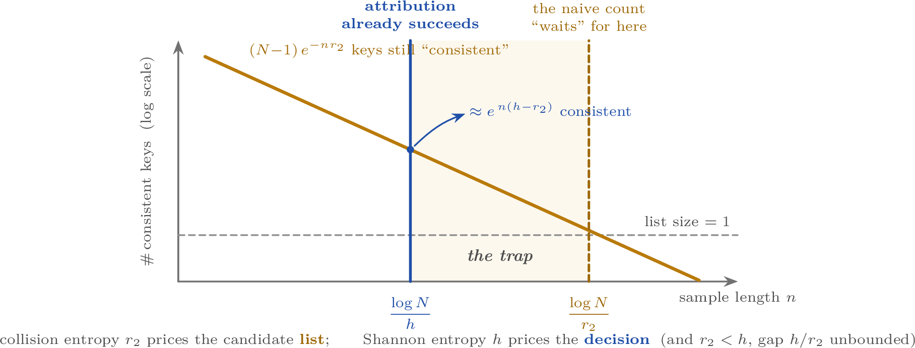
Example 1 (A skewed coin makes the gap concrete). Take \(p_{\mathrm{nat}}=\mathrm{Ber}(0.1)\) i.i.d.(the source of 3.6). Its entropy rate is \(h=H_{\mathrm{b}}(0.1)=0.325\) nats, while its Rényi-2 rate is \(r_2=-\log(0.1^2+0.9^2)=0.198\) nats, so \(h/r_2\approx1.64\). To attribute among \(N=2^{32}\) users, the surprisal threshold succeeds at \(n\approx\log N/h\approx68\) tokens (the \(\log(1/\delta)\) term, about \(9\) tokens here, is lower-order in \(N\)), while the consistency list clears only at \(n\approx\log N/r_2\approx112\); their ratio is exactly \(h/r_2\approx1.64\). The gap grows without bound as the coin skews (\(h/r_2\to\infty\) as \(p\to0\)): the trap is not a constant-factor nuisance.
Credit, again. The false-positive mechanism in (i) is the folklore likelihood-ratio Markov bound, for which we claim no novelty (10.6). What is new is the closed column: the matching achievability at full stationary-ergodic generality (SMB only), with an exact non-asymptotic false-positive side, and its forensic reading — the entropy mass of [thm:budget](b) is operational, not merely a ceiling. The distortion-free sub-column of 1, a one-sided converse ledger in the first version of this paper, is now two-sided at Levels 1 and 2. The closest cryptographic tracing of many adaptive users gives no tight information-theoretic \(h\)-rate [9]; Christ–Gunn-style undetectable schemes are computational and governed by seed entropy (scope note after [thm:budget] in 10). The witness decoder is exact-alignment, hence not edit-robust; a \(\Delta\)-free, edit-robust attribution rate remains open (6).
Remark 9 (Where the columns meet). The two extremal columns of 1 touch at exactly one source. On a full-alphabet-uniform i.i.d.source, \(h=\log q\), so the closed entropy column gives \((1+o(1))\log N/\log q\): the invisible distortion-free witness then costs no more than the cleartext digit-stamp of [thm:dichotomy](b), and only there, since \(\log N/h\ge\log N/\log q\) always, with equality iff \(p_{\mathrm{nat}}=\mathrm{Unif}(\Sigma)\); the witness moreover saturates [thm:budget](b) with equality (\(I(K;X)=H(X)=nh_n\) for the deterministic sampler), which is why the column closes. Separately, the collision trap vanishes exactly on support-uniform sources (\(r_2=h\) iff \(p_{\mathrm{nat}}\) is uniform on its support, 8(iii)): the overcharge \(h/r_2\) is a price of skew. The two degeneracies are distinct: a source uniform on a strict sub-alphabet kills the trap but not the gap between the columns.
| Level | Task | Distributional \(\mathcal B(\Delta)\) (\(h\): distortion-free) | Footprint \(\mathcal E(m)\) (embedding) |
|---|---|---|---|
| 0 | Detection | \(\Theta(1/\Delta)\) / \(\Theta(\lambda/h)\) | same (baseline) |
| 1 | Attribution (\(N\)) | \(\Omega(\log N/\Delta)\,[\Theta\text{ if mixing}]\) / \(\Theta(\log N/h)\) | \(\Theta(\log N/\log q)\), \(\Delta\)-free |
| 2 | Extraction (\(\ell\)) | \(\Omega(\ell/\Delta)\,[\Theta\text{ if mixing}]\) / \(\Theta(\ell/h)\) | \(\Theta(\ell/\log q)\), \(\Delta\)-free |
| 3 | Localization (res.\(w\)) | needs full support, \(w\Delta\ge\log(n/w)\) | coarse \(w=\omega(1)\) only |
3.5 Level 3, and a shared budget↩︎
The top rung, localization, is where the framework does work the budget alone does not predict. A watermark is localizing if it can name which sub-region carries the mark, and the demanding version asks this to survive cropping. Model a crop adversary that deletes all but a contiguous window \(W\) of length \(w\); a scheme is \(w\)-crop-robust if the detector succeeds on \(x_W\) for every offset. We assume the scheme is \(r\)-local / edit-based (3): the marked carrier agrees with an unmarked one outside an \(r\)-neighbourhood \(R^{+}\) of the carrier footprint \(R\) (the support of the edit coupling; for a scheme in \(\mathcal{E}(m)\) over a factorizing source one may take \(R=T\)), the post-hoc regime of image, audio, and patch watermarks, where Level-3 localization is actually studied. Robustness is the one property that is not a functional of \(\nu\) alone: mass and shape live in \(\nu\); crop-robustness additionally needs the edit coupling on \(R\), which is why 3 is stated on the carrier.
theoremThmCrop Under 3, any \(w\)-crop-robust scheme has dilated support \(R^{+}\) meeting every length-\(w\) window; since \(|R^{+}|\le(2r+1)|R|\), its carrier footprint \(|R|\) obeys \[|R|\,w\;\ge\;\frac{n-w+1}{2r+1},\qquad\text{i.e.}\qquad |R|\,w=\Omega(n)\;\;(r=O(1)),\] the \(\Omega(n)\) reading trivial for \(w>n/2\) (a nonempty \(R\) already gives \(|R|\,w>n/2\)). For a scheme in \(\mathcal{E}(m)\) whose natural law factorizes across positions (in particular i.i.d.; the post-hoc regime of 3) one may take \(R=T\), so \(|R|\le m\) and the bound reads \(m\,w=\Omega(n)\). Consequently (i) a small-footprint embedding scheme (\(m=o(n)\), hence \(|R|=o(n)\)) is crop-robust only at coarse resolution \(w=\omega(1)\), and (ii) constant-resolution crop-robustness forces \(|R|=\Omega(n)\), i.e.full support, that is, biasing. Moreover (iii) under 1, for a natural law that factorizes across the length-\(w\) blocks (in particular i.i.d., and the whitened regime of the post-hoc schemes 3 targets), \(w\)-crop-robust localization (naming the window among the \(\Theta(n/w)\) blocks from \(x_W\) alone) requires \(w\Delta\ge(1-o(1))\log(n/w)\).
Proof sketch. If a length-\(w\) window \(W\) misses \(R^{+}\), then by the coupling of 3 \(x_W=x'_W\sim p_{\mathrm{nat}}\), so a detector seeing only \(x_W\) tests \(p_{\mathrm{nat}}\) against \(p_{\mathrm{nat}}\) and cannot beat chance, a contradiction. Hence \(R^{+}\) meets every length-\(w\) window; there are \(n-w+1\) such windows and one element pierces at most \(w\) of them, so \(|R^{+}|\ge(n-w+1)/w\); with \(|R^{+}|\le(2r+1)|R|\) this gives \(|R|\,w=\Omega(n)\), and \(|R|\le m\) for \(\mathcal{E}(m)\). For (iii), partition \([n]\) into \(N_w=\lfloor n/w\rfloor\) disjoint length-\(w\) blocks; naming the surviving block is attribution among the blocks ([thm:separation] with the \(N_w\) blocks as users), so by Fano \(I(J;x_{W_J})\ge(1-o(1))\log N_w\) for \(J\sim\mathrm{Unif}[N_w]\). When \(p_{\mathrm{nat}}\) factorizes across the blocks, the golden formula bounds \(I(J;x_{W_J})\le \mathbb{E}_J\sum_{i\in W_J}d_i=\tfrac1{N_w}\sum_{i}d_i\le n\Delta/N_w=w\Delta\), using only the global budget \(\sum_i d_i\le n\Delta\) (no per-token cap); hence \(w\Delta\ge(1-o(1))\log(n/w)\). For correlated \(p_{\mathrm{nat}}\) the cropped block marginalizes its prefix and this accounting can fail; the relation persists in our numerical search, but a tight general proof is left open. ◻
![Figure 8: Why a small footprint cannot localize at fine resolution ([thm:crop]). Under the editcoupling (3), a crop window that misses the dilated footprint R^{+} sees text distributedexactly as p_{\mathrm{nat}}, so a detector reading only that window tests p_{\mathrm{nat}} against p_{\mathrm{nat}} and cannot beatchance. Every length-w window must therefore meet R^{+}, which forces the marks no more than w apart:|R|\,w=\Omega(n). Few marks buy only coarse resolution; fine resolution forces full support, that is,biasing.](/article/2607.13003/_pdflatex/pdtgufym.png "fig:")
So Level 3 turns on a different axis than the footprint (8): a small-footprint embedding scheme cannot be crop-robust at fine resolution at all (a single splice removes its mark), whereas crop-robust fine localization forces full support \(|R|=\Omega(n/w)\). A scheme localizes when it reads a full-support mark at fine per-region resolution and self-locates at window budget \(w\ge\log(n/w)/\Delta\). This is the structural form of the empirical split (fine-readout schemes localize; global-readout schemes do not), made precise in 4.
Finally, the levels are not independent obligations but draws on one account.
propositionPropRegion Under 1 and in the regime \(n\Delta\to\infty\), with \(R_{\mathrm{att}}=\log N\) and \(R_{\mathrm{ext}}=\ell\log2\):
(Converse.) vanishing-error attribution and extraction force \(R_{\mathrm{att}}+R_{\mathrm{ext}}\le (1+o(1))\,n\Delta\);
(Achievability.) for regular, strongly-mixing \(p_{\mathrm{nat}}\) (general \(q\)-ary conjectural, inheriting [thm:dichotomy](a)), every pair with \(R_{\mathrm{att}}+R_{\mathrm{ext}}\le(1-o(1))\,nC\) is achieved by one multiplexed conditional tilting code, where \(C=\Theta(\Delta)\) is the per-token channel capacity.
Thus the achievable region is a slope-\(-1\) simplex whose boundary is order-tight, \(\Theta(n\Delta)\): it lies between \(nC\) and \(n\Delta\), which agree up to the capacity constant (\(C\approx\Delta/4\) in the binary witness of 3.6). The corners carry no extra loss.
Proof sketch. With \(S=(U,W)\), the chain rule gives \(I(U,W;X)=I(U;X)+I(W;X\mid U)\le n\Delta\) ([thm:budget]); Fano on \(U\) and conditional Fano on \(W\mid U\) make the two terms \(\ge(1-o(1))R_{\mathrm{att}}\) and \(\ge(1-o(1))R_{\mathrm{ext}}\), giving (a). For (b), concatenate the two messages into one codeword and apply [thm:dichotomy](a) at rate \(nC\). ◻
So it is not just that attribution and extraction are each \(\Omega(\cdot/\Delta)\), but that a biasing watermark cannot be cheap at both at once: every nat spent naming the user is a nat denied to the payload (9). The embedding analogue is the \(\Delta\)-free simplex \(R_{\mathrm{att}}+R_{\mathrm{ext}}\le m\log q\), now a theorem ([thm:budget](c), the \(L^0\) face of the mass cap), and there, uniquely, the bound is constant-exact (the zero-error stamp readback meets it).
![Figure 9: Two rate regions, one shape ([prop:region]). Attribution and extraction draw on thesingle budget of [thm:budget], so their rates trade off along a slope-(-1) frontier. (a) Underthe per-token cap \mathcal{B}(\Delta) the frontier is soft, order-tight \Theta(n\Delta), lying between theachievable nC and the converse n\Delta (C\approx\Delta/4 in the binary witness of 3.6).(b) Under the footprint cap \mathcal{E}(m) it is sharp and constant-exact, R_{\mathrm{att}}+R_{\mathrm{ext}}=m\logq, met with equality and zero error by the stamp. The same simplex, with a soft boundary on one side and ahard one on the other.](/article/2607.13003/_pdflatex/pzbetldk.png "fig:")
3.6 Numerical illustration↩︎
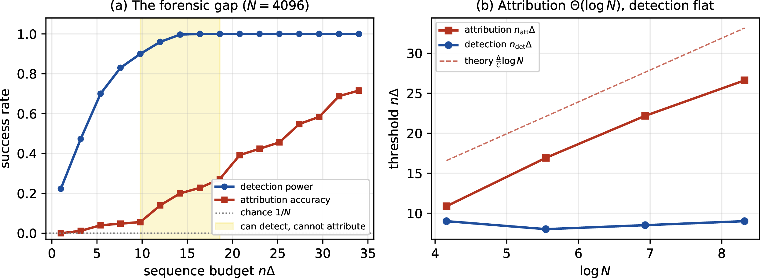
We instantiate the tilting code over a binary alphabet (\(p_+=\mathrm{Ber}(\tfrac12+s)\), \(p_{\mathrm{nat}}= \mathrm{Ber}(\tfrac12)\)) and measure detection power and attribution accuracy by seeded Monte Carlo (10). Three findings confirm the theory. (i) The converse 1 is never violated. (ii) The attribution threshold scales as \(\log N/C\), where \(C=I(b;X)=\Theta(\Delta)\) is the channel capacity (empirically \(C\approx\Delta/4\) at \(s=0.08\), so the operative constant is the capacity, not \(\Delta\) itself), and grows by exactly the factor \(\log4096/\log64=2\) as \(N\) goes from \(64\) to \(4096\), while the detection threshold is flat in \(N\), so the ratio is \(\Theta(\log N)\) (10b). (iii) At \(N=4096\), detection power is already \(0.99\) while attribution accuracy is still \(0.28\) at a common length (\(n=1400\); 10a), and detection saturates to \(1.00\) several hundred tokens before attribution leaves chance (it reaches \(0.55\) only at \(n=2200\)): the finite-\(N\) form of the gap. The embedding stamp, by contrast, attributes among all \(4096\) users from \(n=12\) tokens, where the biasing scheme is at chance. The first two findings quantify [thm:separation]; the third quantifies [thm:dichotomy].
Two further seeded experiments exercise [thm:entropyclose] directly. The first runs the threshold decoder on an i.i.d.binary source (\(h\approx0.325\), \(r_2\approx0.198\)) at \(\delta=0.05\) and \(N\) up to \(2^{32}\): the per-innocent false-positive rate satisfies \(\mathrm{FP}\cdot N/\delta\le0.11\) at every tested length, including the boundary \(n=\tau/h\), while the consistency-only decoder (no surprisal threshold) overshoots the \(\delta/N\) target by one to four orders of magnitude — the collision trap of 8, priced by \(e^{-nr_2}\), not by the decision rate. A companion run tracks the consistency decoder’s threshold drift (seeded) and supports the abstain-on-tie completeness observation of 8. The second checks the Jensen step, \(\mathbb{E}_\kappa[H(\hat{p}_\kappa)]\le nh_n\), at all tested \((n,N)\) pairs, including \(N>e^{nh}\) (all pass). All runs are seeded and reproducible.
3.7 Confirmation on deployed language models↩︎
The theory makes a falsifiable numerical prediction: the consistency rule’s overcharge is the entropy ratio \(h/r_2\), a quantity fixed by the source and by nothing about the watermark. On natural language it should be a stable constant near \(1.6\). The binary source of 3.6 isolates the mechanism on a distribution we control; we now close the loop, measuring \(h/r_2\) and the detection/attribution thresholds where they are meant to bite: on real autoregressive language models, and on the watermarks practitioners deploy. These are illustrations of the theory’s operational content, not new theory — the lower bounds remain the theorems, unfalsifiable by simulation, and what follows measures their inputs (the rates \(h,r_2\) and the detection/attribution thresholds) on real systems; the exact false-positive guarantee \(\delta/N\) itself was exercised in the seeded numerics of 3.6. All experiments are seeded and reproducible.
3.7.0.1 The collision trap on a shipped distortion-free scheme.
[thm:entropyclose] and its trap (8) live in the distortion-free regime, whose deployable instance is the exponential-minimum-sampling (Gumbel-max) watermark of [21] and [13]: a key-seeded Gumbel perturbs the logits, \(x_t=\arg\max_i\bigl(\log p_{\mathrm{nat}}(i\mid x_{<t})+g^{(\kappa)}_{t,i}\bigr)\), so marginally \(x_t\sim p_{\mathrm{nat}}\). We run it on GPT-2 [22]. Two properties make the entropy column apply, and we verify rather than assume both. (i) Distortion-free: the marked text has the same Shannon and Rényi-2 rates as unmarked sampling (\(h=3.81\) vs.\(3.76\), \(r_2=2.36\) vs.\(2.33\) nats/token), so the mark spends no distortion. (ii) The collision is real: at a fixed context, \(8000\) independent keys reproduce \(p_{\mathrm{nat}}\) (its \(20\) most likely tokens to within \(0.006\)), so an innocent key emits token \(v\) with probability exactly \(p_{\mathrm{nat}}(v)\) — so the per-token collision law of 8 is a property of the construction at a fixed context, not a modelling assumption (\(r_2\) here is the empirical Rényi-2 rate, and the \((N-1)e^{-nr_2}\) count is its per-token extrapolation). The guarantee lengths then separate as predicted (11): implicating no innocent above \(\delta/N\) costs \(\log(N/\delta)/r_2\) tokens under the consistency rule but only \(\log(N/\delta)/h\) under surprisal thresholding, a ratio \(h/r_2=1.61\) on GPT-2. This is the trap on a scheme one can ship, and the deterministic witness of 3.6 recovers the very same constant.
![Figure 11: The collision trap on the deployed EMS (Gumbel-max) distortion-free watermark, GPT-2. (a) The marked text’s Shannon (h) and Rényi-2 (r_2) rates coincide with unmarked sampling (dotted): the watermark is distortion-free, so the entropy column of [thm:entropyclose] applies. (b) To implicate no innocent user above \delta/N, the consistency-list rule needs \log(N/\delta)/r_2 tokens (amber) while surprisal thresholding needs \log(N/\delta)/h (blue); the shaded overcharge is the factor h/r_2=1.61, widening as \Theta(\log N).](/article/2607.13003/figures/exp-ems.png "fig:")
3.7.0.2 Detection is not attribution, on the deployed green-list.
The green-list of [2] is the extremal biasing profile (the \(\mathcal{B}(\Delta)\) column of [thm:dichotomy]): a context-keyed split greens a fraction \(\gamma=\tfrac14\) of the vocabulary and adds a fixed logit bias (here \(2.0\)). On GPT-2 the realized green fraction is \(0.62\) under the true key against \(0.25\) under any innocent key. 12 exhibits [thm:separation] in finite-\(N\) form: detection power saturates by \(n\approx28\) tokens independently of \(N\), whereas the attribution length (here the \(50\%\)-accuracy crossing) grows linearly in \(\log N\) (\(+2.3\) tokens per doubling, from \(16\) to \(61\) tokens as \(N\) runs \(2^{8}\) to \(2^{28}\)). Between the two lies a window in which the passage is detectable yet unattributable. Unlike the EMS scheme above, the green-list shifts the entropy: the two quality models of 1, the same separation read off either column.
![Figure 12: Detection is not attribution on the deployed green-list watermark, GPT-2. (a) Detection power saturates by n\approx28 tokens while attribution accuracy (shown for N=2^{20}) lags; in the shaded window the text is detectable yet unattributable. (b) The attribution length (the 50\%-accuracy crossing) grows linearly in \log N (+2.3 tokens per doubling of N); the detection threshold is flat in N. The finite-N form of the \Theta(\log N) gap of [thm:separation].](/article/2607.13003/figures/exp-greenlist.png "fig:")
3.7.0.3 The overcharge is a property of language, not of one model.
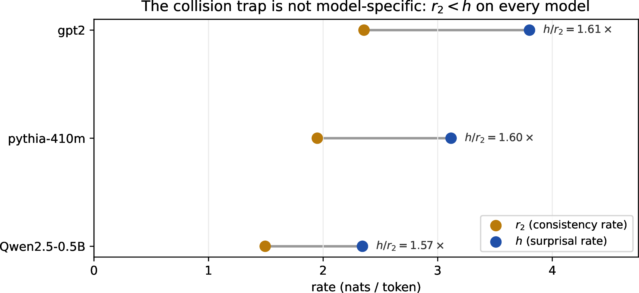
The constant \(h/r_2\) is the only model-dependent quantity in the trap, so we measure it across families. On GPT-2, Pythia-410M [23], and Qwen2.5-0.5B [24] — three pretraining corpora and tokenizers, vocabularies from \(50\)k to \(152\)k — the absolute rates fall as the models sharpen (\(h\) from \(3.80\) to \(2.34\) nats/token), but the overcharge is stable: \(h/r_2=1.61,\,1.60, \,1.57\) (13). The collision trap reflects the gap between the Shannon and Rényi-2 rates of natural language, not an artifact of any one model.
4 The framework applied: a taxonomy of deployed watermarks↩︎
The classification of 1 is decided by one measurable quantity: the per-secret footprint \(T\) (the reading set: the positions on which the per-secret kernels are marked, [cor:bridge]), read in the basis the extractor works in. The per-secret reading is not optional: the key-averaged support would misclassify every distortion-free scheme as \(\mathcal{E}(0)\), since averaging over the key can erase a mark present under every individual key (parity witness, 10.8). ¿tbl:tab:taxonomy? evaluates the criterion on twenty-one representative schemes (the twenty deployed watermarks and the theoretical digit-stamp witness), holding it fixed (so a scheme is embedding only if its per-secret kernels truly mark \(o(n)\) coordinates, not merely if its secret is readable from a sub-carrier); 11 works through each scheme individually. Two axes turn out to matter, and they are orthogonal: the footprint \(T\), which governs the embedding/biasing split and the \(\Delta\)-free decoupling of [thm:dichotomy]; and the readout resolution, whether the mark is decoded globally or per-region, which governs Level 3. Three patterns follow.
![Figure 14: The two orthogonal axes of the taxonomy. The footprint |T| (horizontal; small gold dots= embedding, full-support blue dots = biasing) governs the \Delta-free decoupling of[thm:dichotomy]; the readout resolution (vertical) governs localization ([thm:crop]). Beingindependent, the two axes let deployed schemes spread across three quadrants, and the localizers (SEAL,EditGuard, AudioSeal) reach Level 3 by fine readout, not a small footprint. The fourth quadrant, smallfootprint with fine resolution, is empty for a reason: [thm:crop] forbids it, m\,w=\Omega(n).](/article/2607.13003/_pdflatex/pfdvwsjm.png "fig:")
4pt
@lllllll@ Scheme & Basis & Footprint & Model & Readout & Levels & Class
Green-list [2] & tokens & full & \(\mathcal B(\Delta)\) & global &
0,(1,2) & biasing
Unigram [25] & tokens & full & \(\mathcal B(\Delta)\) & global & 0 & biasing
SynthID-Text [15] & tokens & full & d-free & global & 0 & biasing (d-free)
Reweighting [26], [27] & tokens & full & d-free & global
& 0 & biasing (d-free)
Multi-bit [28], [29] & tokens & full & \(\mathcal B(\Delta)\)/d-free & bucketed & 0,2 & biasing
BiMark [30] & tokens & full & d-free & bucketed & 0,2 & biasing (d-free)
Many-user [9] & tokens & full & d-free & global & 0–2 & biasing (d-free)
Distortion-free [13] & tokens & full & d-free & global & 0 & biasing (d-free)
Undetectable [6] & tokens & full & d-free & global & 0 & biasing (d-free)
PRC [14] & tokens & full & d-free & global & 0 & biasing (d-free)
SemStamp [31] & sentence-emb. & full & \(\mathcal B(\Delta)\) & global & 0 &
biasing
Tree-Ring [1] & Fourier & small & d-free & global & 0,(1) & embedding
RingID [32] & Fourier & full & d-free (part.) & global & 0,1 & biasing
Gaussian Shading [33] & latent & full & d-free & global & 0,2 & biasing (d-free)
ROBIN [34] & Fourier (interm.) & full & \(\mathcal B(\Delta)\) & global & 0 &
biasing
HiDDeN [35] & pixels & full & \(\mathcal B(\Delta)\) & global & 0,2 & biasing
Stable Signature [36] & feature & full & \(\mathcal B(\Delta)\) & global &
0,2 & biasing
SEAL [19] & latent & full & d-free & fine & 0–3 & biasing (d-free)
EditGuard [20] & pixels & full & \(\mathcal B(\Delta)\) & fine & 0,(2),3
& biasing
AudioSeal [37] & samples & full & \(\mathcal B(\Delta)\) & fine
& 0,(2),3 & biasing
(Digit-stamp, [thm:dichotomy](b)) & tokens & small & \(\mathcal E(m)\) & global & 0–2 &
embedding
4.0.0.1 1. Almost every deployed watermark is biasing, and the \(\Delta\)-free class is nearly empty.
Applied consistently, the footprint criterion puts not only the LLM schemes but also the neural image and audio watermarks on the biasing side: green-list and its descendants tilt every token; the distortion-free family keeps \(\bar p=p_{\mathrm{nat}}\) but spreads its signal over the whole sequence; and SEAL, EditGuard, AudioSeal, and Stable Signature perturb the entire latent, image, or waveform. For the distortion-free rows the per-secret reading shows this is forced, not incidental: the per-secret kernels of an exact sampler are near-deterministic in the key (each conditional collapses onto the token the key selects), so every position is marked (full support), and the per-token conditional divergence exceeds any finite cap, placing these schemes outside \(\mathcal{B}(\Delta)\) for every finite \(\Delta\). They are governed by the entropy column, and by [thm:entropyclose] that column is now closed: attribution among \(N\) users at \(n=(1+o(1))\log N/h\) is tight for the exact-sampler schemes with i.i.d.keys that the theorem covers (the computationally undetectable constructions, governed by seed entropy, sit outside its hypotheses). The only genuine \(o(n)\)-footprint schemes in ¿tbl:tab:taxonomy? are Tree-Ring (a ring on a few Fourier shells) and the theoretical digit-stamp. Even RingID [32], the Tree-Ring successor engineered for multi-key identification, does not join them: its key capacity comes from a key-specific noise pattern occupying an entire latent channel alongside the discretized rings, so its per-secret footprint is a constant fraction of the latent (11) — attribution capacity was bought by leaving the small-footprint class. The \(\Delta\)-free decoupling of [thm:dichotomy](b) is therefore realized by essentially no deployed scheme, which is precisely why deployable, edit-robust \(\Delta\)-free attribution is open (6), not a solved case we are merely cataloguing.
4.0.0.2 2. Localization is a second, orthogonal axis (readout resolution), and the framework predicts its cost.
Whether a scheme reaches Level 3 is decided not by its footprint but by whether its (full-support) mark is decoded per-region: SEAL reads a per-patch hash, EditGuard a per-region mask, AudioSeal a per-sample residual, while green-list reads one whole-passage count. This is not in tension with [thm:crop]; it is its content. Crop-robust localization at resolution \(w\) requires a carrier footprint of size \(\Omega(n/w)\), so a scheme that localizes finely and survives cropping must be full-support. The deployed localizers are indeed observed to be full-support (¿tbl:tab:taxonomy?), consistent with this. The framework thus predicts both halves of the empirical benchmark on which fine-readout embedding-style schemes localize at high AUC while global-readout latent schemes (Gaussian Shading, Tree-Ring in pixels) score near zero [19].
4.0.0.3 3. The classification is basis-relative.
Tree-Ring is the one deployed embedding scheme, and only in the right basis: in the latent-noise spatial basis the inverse-DFT of the ring spreads over all noise coordinates (and the noise-to-image map is the full diffusion sampler, not a transform), so there it is biasing; in the Fourier basis of the initial noise the mark is a small object on a few frequency shells, and the detector reads it there by inverting the generation.1 The localization map can be a change of basis; the framework asks in which representation the mark becomes an \(o(n)\) object, and answers that for almost all of today’s schemes there is none. SemStamp [31] makes the relativity concrete a second time, in the opposite direction: its extractor reads a sentence-embedding dictionary, where the carrier’s coordinates are sentences rather than tokens, and the basis change re-grains the footprint without shrinking it: every sentence is steered into a keyed LSH region, so the scheme is full-support at either granularity. A change of basis can relocate the mark (Tree-Ring) or merely change the units in which it is read (SemStamp); only the former creates an \(o(n)\) object.
4.0.0.4 Consistency with the definition.
A green-list key is recoverable from a long window and a SEAL patch-hash is readable from a crop, yet both schemes mark a constant fraction of coordinates under every key, so both are biasing under the per-secret footprint (1); they differ in readout resolution, not in footprint. Keying the embedding/biasing line on “readable from a sub-carrier” would split them; keying it on the footprint does not, and ¿tbl:tab:taxonomy? is the consistent application.
5 Related work↩︎
5.0.0.1 Detection statistics (Level 0), imported.
A line of recent work pins down the sample complexity of watermark detection. [3] give uniformly most powerful tests and matching minimax Type-II bounds; [4] derive closed-form detection efficiency and the pivotal statistic; [5] establish the per-step KL detectability floor \(1-\sqrt{1-e^{-D_{\mathrm{KL}}}}\) and the fidelity–detectability frontier (sharpened by [38] to a tight \(f\)-divergence bound). These fix our Level-0 rung at \(n_{\mathrm{det}}=\Theta(1/\Delta)\); we treat the rate and the \(\Delta\!\leftrightarrow\!(\alpha,\beta)\) knob as given and build the ladder above them.
5.0.0.2 Multi-user watermarking and fingerprinting (Level 1).
[9] construct language-model watermarks for many adaptive users with a detect-short / trace-long gap, built from Tardos and Boneh–Shaw fingerprinting codes [39], [40]. This is the closest prior art, and it proves the direction complementary to ours: achievability of cheap detection with expensive tracing in a cryptographic model. Their sole optimality remark is a counting argument (“\(\log n\) bits are needed to identify a user”); there is no statistical converse on length, no distortion budget, and no biasing side. The matching converse we use is not new: the distortion-constrained fingerprinting converse of [7] and [8] already proves that fingerprinting capacity under a fidelity constraint \(\to0\) as the constraint tightens, exactly the “couples to the budget” phenomenon (with \(L_2\)-distortion in place of KL). We import it and instantiate it for the per-token KL channel rather than claim it. Classical fingerprinting [39] supplies the \(\Theta(c^2\log N)\) scaling under the combinatorial marking assumption (the same code machinery drives tight lower bounds well beyond watermarking, e.g.in differential privacy, [41]), but with no detection task and hence no separation. Our addition over this line is the contrast with the footprint model ([thm:dichotomy]), not the converse. [10] study detection versus attribution empirically at fixed length and argue, under a strict threshold, that the two essentially coincide. This is the opposite phenomenology to our impossibility regime, which their model (embedding bitstrings, no biasing, no length law) cannot express. Concurrent work of [42] studies attribution faithfulness without a sample-complexity ladder. On the deployed-attribution axis, [43] recover a membership/identity signal from watermarked text (“radioactivity”); this is a Level-1-flavored capability in practice, but it asks whether a model was trained on marked text rather than which of \(N\) users emitted a fixed sample, and it carries no length law. Multi-bit payload capacity (Level 2) is studied by [44] via Gelfand–Pinsker coding and by [28], [29]; our embedding-side payload term is consistent with these, and the \(\log N\) attribution surcharge is the axis they lack.
5.0.0.3 The embedding/biasing taxonomy (Level 3 and the dichotomy).
The recent SoK [11] taxonomizes “statistical” (token-probability) versus “embedding” (content-feature) schemes and argues detection and attribution should be separate functions, but on the robustness-versus-unforgeability security axis, with no sample-complexity content; the statistical/embedding split there is an engineering taxonomy, never a theorem or a phase boundary. Empirical localization results confirm the mechanism without explaining it: SEAL [19] localizes at \(98.2\%\) AUC where distributional schemes score \(0\%\) on the same task, and EditGuard [20] gives tamper localization for image watermarks. Our [thm:dichotomy] is, to our knowledge, the first theorem stating the existence of a localization map as the boundary between \(\Delta\)-coupled and \(\Delta\)-free forensic cost.
5.0.0.4 Concurrent information-theoretic frameworks.
Distributional Information Embedding [12] is the closest concurrent framework: it analyzes the watermarking trade-off at the level of the scalar \(\mathop{\mathrm{I}}(S;X)\). Our profile \(\nu(t)\) is the positional refinement of that scalar (its mass recovers it), and the forensic ladder is the use the refinement is put to: tasks become functionals of \(\nu\) that a single number cannot separate. The unified-optimization framework of [45] treats scheme design as constrained optimization, the design axis, orthogonal to sample complexity. Proportion estimation [46] targets a different Level-3-adjacent estimand: what fraction of a text is marked, not which positions; WISER [47] localizes multi-segment watermarks via change-point methods, an empirical/finite-sample method with no information-theoretic lower bound.
5.0.0.5 Steganography.
The information-theoretic model of steganography [16], [48] and the square-root law of steganographic capacity [49] concern the bounded-total-KL regime, where keeping the total divergence constant forces an embeddable payload of order \(\sqrt n\). Our regime is the linear-total-KL one: a per-token budget \(\Delta\) gives total budget \(n\Delta\) and a payload linear in \(n\). The two should not be conflated; the forensic-recovery budget ([thm:budget]) is the linear-regime analogue of the stego capacity bound, now resolved by forensic level and by mechanism. The structurally closest predecessor of a per-position information quantity is [50]: under mutually independent embedding, a per-element Fisher information, summed across the cover, determines the capacity of \(\varepsilon\)-secure steganography — the engine of the square-root law. The profile \(\nu\) differs on three axes: it is a mutual-information quantity, not a second-order (Fisher) one; it feeds per-task functionals (mass and shape), not a single aggregate capacity; and it is defined on autoregressive conditionals, not i.i.d.cover models.
5.0.0.6 Covert communication and perfect steganography.
The square-root law of covert capacity [51]–[53] lives in the budget regime \(\mathop{\mathrm{KL}}\le\varepsilon\): a fixed total divergence forces an \(O(\sqrt n)\) payload. The statistically distortion-free column of 1 is the \(\mathop{\mathrm{KL}}=0\) keyed regime (Cachin-style perfect steganography [48]) where the binding resource is not a divergence budget but the generation entropy \(h\). [thm:entropyclose] is the multi-user attribution rate for that regime; to our knowledge no prior work gives a tight \(h\)-rate for \(N\)-user attribution. The closest, [9], is cryptographic (security-parameter counting, with adaptive robustness as the focus), complementary, not rate-tight.
5.0.0.7 Identification via channels.
[54] cast watermark identification as identification via channels in the sense of [55]: the blocklength is held fixed and the number of verifiable signatures grows doubly exponentially in it. This is the dual of our question, which fixes the user population \(N\) and asks for the sample cost \(n(N)\). Their split between verification (“is it signature \(s\)?”) and decoding (“which signature?”) has, to our knowledge, no sample-complexity counterpart; we pose it as an open question in 6.
5.0.0.8 Impossibility and robustness.
A separate thread shows strong watermarks can be removed under mild assumptions [56], [57], the latter giving a sharp coding-theoretic ceiling on tamper robustness, and that reusing a detector across keys inflates false positives [58]; on the attack side, [59] exhibit statistical-to-computational gaps for removal. The false-detection result is a \(\Delta\)-dependent upper bound on one parasitic detector, not a floor over all detectors on natural content; we discuss the corresponding open question (a false-positive floor) in 6. Recent design, detection, attack, and localization work adjacent to the framework is surveyed further in 12.
6 Discussion↩︎
6.0.0.1 What the dichotomy says for regulation.
Current statutes ask for marks “in a machine-readable format” (EU AI Act, Art. 50), “noticeable labels” (China’s Deep Synthesis provisions), or “latent disclosure” (California SB 942). Read operationally, each presumes an extractable object: the embedding side of 1. [thm:dichotomy] makes the cost of that presumption precise: a biasing watermark can satisfy a Level-1 (attribution) or Level-2 (extraction) mandate only at a sample cost \(\Omega(\log N/\Delta)\) that diverges as the mark is made stealthier (\(\Delta\to0\)), whereas an embedding watermark pays a fixed \(\Theta(\log N/\log q)\) independent of fidelity. A regulator who wants attribution is, whether or not the text says so, mandating the embedding ontology. We state this as an informed structural consequence, not a legal interpretation.
6.0.0.2 Which rate is a sample complexity.
The closed column also settles a question the naive analysis gets wrong: the Rényi-2 rate \(r_2\) governs the size of the falsely-consistent list, but the Shannon rate \(h\) governs the decision, and only the decision is what a forensic guarantee names (8). Whether an edit-robust decoder, which can no longer check consistency token-for-token, is forced back onto the larger \(r_2\) rate is the open question we turn to next.
6.0.0.3 Localization (Level 3) and the witness gap.
[thm:crop] makes the redundancy–resolution tradeoff quantitative: crop-robust localization at resolution \(w\) forces \(m\,w=\Omega(n)\) (precisely \(|R^{+}|\ge(n-w+1)/w\) for the dilated support and \(|R|\ge|R^{+}|/(2r+1)\), with \(|R|\le m\) in the factorizing regime). This explains the empirical split (4) and exposes the honest limit of our decoupling witness. The digit-stamp of [thm:dichotomy](b) has footprint \(m=\Theta(\log N/\log q)=o(n)\), so by [thm:crop](ii) it cannot be crop-robust at any fine resolution: a single splice destroys it. The deployed schemes that do localize (SEAL at \(98.2\%\) AUC, EditGuard, AudioSeal) are, by [thm:crop], forced to be full-support; they are biasing and localize only because they read their delocalized mark at fine per-region resolution. So the clean \(\Delta\)-free decoupling and operational edit-robust localization pull in opposite directions, and the question our witness leaves open (is there a deployable (imperceptible, edit-robust) scheme whose attribution cost is \(\Delta\)-free?) is, by [thm:crop], exactly the question of whether one can be \(\Delta\)-free on the payload while paying the \(m\,w=\Omega(n)\) tax only on the locating layer. We conjecture this is achievable with a layered PRC-style construction but do not prove it. The same gap is now the live one on the distortion-free side: [thm:entropyclose] closes the attribution rate there, but its witness decoder is exact-alignment (consistency is checked token-for-token against the key) and a single edit destroys it. Under a soft (edit-robust) notion of consistency the true key is no longer deterministically consistent, the tie-abstention device behind 8 loses its zero-false-positive guarantee, and a genuine \(r_2\)-type cost may resurface. Whether edit-robust distortion-free attribution still costs \(\log N/h\), or genuinely pays the larger \(\log N/r_2\), is the sharpest open problem the framework raises.
6.0.0.4 Verification versus search (open).
Our attribution task is a search: which of \(N\) users emitted \(X\)? The verification variant (is it user \(u\)?) is a composite binary test, and the identification-via-channels literature [54], [55], with a covert (distortion-free) analogue in [60], suggests the two scale very differently: at fixed blocklength the number of verifiable signatures is doubly exponential while the decodable ones are merely exponential. The sample-complexity dual would make verification \(N\)-free, an exponential separation from search’s \(\Theta(\log N/\Delta)\); the proof obstacle is testing the composite null (the \(N-1\) other keys) uniformly. The sample-complexity version of the verification-vs-decoding split is open; we have not pursued it here.
6.0.0.5 A false-positive floor (open).
The seed of this work conjectured an information-theoretic false-positive floor for biasing watermarks on natural content: that no detector can drive the false-positive rate to zero at fixed power when \(p_{\mathrm{wm}}\) and \(p_{\mathrm{nat}}\) overlap. Against a computationally unbounded distinguisher this is delicate, since undetectable constructions [6] make the marginal gap vanish, so any floor must be stated in the key-known or information-theoretic-adversary regime. [58] give a related upper bound (false positives inflate when a detector is reused across keys), but a genuine floor over all detectors on a natural-content null remains open. We leave it as a conjecture rather than fold a weaker statement into the main results.
6.0.0.6 Tightness and generality of the achievability (open).
Three gaps remain between our converses and the constructions that meet them. The \(\mathcal{B}(\Delta)\) achievability of [thm:dichotomy](a) matches its converse only up to the per-position capacity constant, and only for memoryless or regular strongly-mixing sources; the exact \(q\)-ary tilting constant, and a general-ergodic achievability that removes the mixing hypothesis the conditional tilting code needs, are both open. On the distortion-free side the entropy column assumes i.i.d.per-user keys; correlated or coded assignments (Tardos-style, [39]) might trade candidate-list size against length, a different point on the same rate curve. None of these changes a rate order; each sharpens a constant or widens a hypothesis.
6.0.0.7 Existence, identity, and the ledger.
Beneath the rates, the ladder separates two kinds of question. Detection asks whether a mark exists: a two-point hypothesis test, whose cost is set by a fixed divergence and is indifferent to the size of the user population. Attribution asks who: an estimation among \(N\) alternatives, which cannot conclude before \(\log N\) nats of identity have arrived. Existence is cheap; identity is priced; and the window of [thm:separation] is what lies between, a text that can raise suspicion but cannot yet support a name. The form of a forensic guarantee matters as much as its rate: [thm:entropyclose](i) prices false accusation per innocent rather than on average (no innocent is implicated except with probability \(\delta/N\), exactly and non-asymptotically), which is the quantitative shape of a presumption of innocence. And the account every level draws on is settled before any question is asked: by data processing ([thm:budget]), reading the carrier can only spend information that generation deposited, never mint more. What can ever be detected, attributed, or extracted from a scheme’s output is fixed, token by token, by the profile \(\nu\) it writes, and where it can be localized is fixed by the shape of \(\nu\) together with the edit coupling on the carrier; the quality models are covenants on the deposits (\(\Delta\) at a time, or only what the source’s entropy affords); attribution and extraction are withdrawals against one balance ([prop:region]). Design is the choice of a deposit schedule, and a forensic mandate is, in the end, a constraint on \(\nu\).
6.0.0.8 Limitations.
(i) Our bounds are information-theoretic: \(\Phi(n)=I(S;X)\) caps every computationally unbounded extractor, so the lower bounds are unconditional, but the distortion-free budget (2) uses statistical undetectability, with a negligible slack under merely computational undetectability. (ii) The Level-0 detection rate we import assumes the standard independent/stationary-token model [3], [4]; our co-located gap needs only that the key-unknown detection error vanishes on the window, which in that model follows from a positive per-token mixture divergence via the relative-entropy ergodic theorem (a large total KL alone would not suffice for a single joint sample). (iii) The within-scheme impossibility ([thm:separation], “detectable yet unattributable at one length”) is an asymptotic statement: it lives on the window \(\omega(1/\Delta)\le n<(1-\eta)\log N/\Delta\), which is wide as \(N\to\infty\) but narrow at moderate \(N\), so our simulations (3.6) accordingly exhibit the robust form of the separation (attribution threshold \(\Theta(\log N)\) above the detection threshold) rather than the razor-thin point. (iv) The embedding “stamp” of [thm:dichotomy] is the simplest witness of decoupling, not a deployable scheme; robust embedding watermarks (commitment- or code-based; SEAL, EditGuard empirically) realize the same decoupling with imperceptibility and robustness, which we cite rather than reprove. (v) The distortion-free achievability of [thm:entropyclose] [cor:extraction-h] is information-theoretic in its decoder as well: the witness extractor searches the key set, so it runs in time \(\Theta(N)=\Theta(2^\ell)\) in the payload; an efficient \(\Theta(\ell/h)\)-sample extractor is a separate requirement, which the “machine-readable mark” reading of a regulatory mandate implicitly wants and which we leave open.
6.0.0.9 Summary.
A watermark is an object in its carrier or a property of its law, and the footprint of 1 is where that informal distinction becomes measurable. Detection is the cheapest question one can ask of either kind, and the only one whose cost is mechanism-blind. Every question above it (who, what, where) is metered by a single distortion budget for schemes confined to the distributional quality model, and bought at a \(\Delta\)-free price by schemes that can use a bounded footprint; the localization map is the structural feature that admits the cheaper model, and it enables without deciding. The three questions above detection are readings of one measure, two of its mass and one of its shape with the edit coupling on the carrier, and their prices differ because the readings do.
7 Conclusion↩︎
A watermark decides, token by token as it generates, how much of its secret the world will ever recover; the information profile \(\nu(t)=I(S;X_t\mid X_{<t})\) is the record of that decision, and the forensic questions above detection are readings of it. The prices follow. The mass \(\norm{\nu}_1\) funds attribution and extraction in one of two currencies, \(\Delta\) per token against a fidelity budget or \(h\) per token against the entropy the source affords; the shape of \(\nu\), with the edit coupling on the carrier, governs localization under the uncertainty \(m\,w=\Omega(n)\); detection is the mechanism-blind baseline beneath them. The question that would have led our list of open problems, a distortion-free achievability to match the entropy converse, is closed by [thm:entropyclose]: attribution costs \((1+o(1))(\log N+\log(1/\delta))/h\) at full stationary-ergodic generality, with an exact per-innocent false-positive guarantee, and extraction follows at \(\Theta(\ell/h)\) ([cor:extraction-h]).
With this the ladder’s currencies are identified at every rung: \(\Delta\), \(h\), and the geometry of the footprint. What the framework leaves open — and the sharpest of it is a matter of robustness, not of information — we set out in 6.
Nothing in the profile is special to watermarking. \(\nu(t)=I(S;X_t\mid X_{<t})\) prices what any secret threaded through a sequential generator makes recoverable, and its mass-versus-shape reading should apply wherever information is embedded position by position — steganography, fingerprinting, covert communication. We have used it to say one thing about one domain: the forensic power of a watermark is fixed by the information it makes recoverable, not by the mechanics of how the mark is embedded.
8 Notation↩︎
[tab:notation] collects the symbols used throughout. The dependency structure of the results is mapped in 3 (3); the imported and textbook facts each proof draws on are catalogued in 10.1 and cited inline at each use. All logarithms and information quantities are in nats unless a base is shown; per the convention of 2, the profile \(\nu\) and the budget \(\Phi\) are read conditional on the registry \(\kappa\) (written \(I(S;X)\) for brevity).
@l @ l @ l@
Symbol & Meaning & Defined in
Symbol & Meaning & Defined in
\(n\) & carrier length (number of tokens) & 2
\(\Sigma,\;q=|\Sigma|\) & token alphabet and its size & 2
\(X\in\Sigma^n\) & the carrier (the generated text/sample) & 2
\(p_{\mathrm{nat}}\) & natural (unmarked) law on \(\Sigma^n\) & 2
\(p_{\mathrm{wm}}^{(k)}\) & marked law under key \(k\) & 2
\(\bar p=\mathbb{E}_K\,p_{\mathrm{wm}}^{(K)}\) & key-averaged (mixture) law & 2
\(K\in\mathcal{K}\) & secret key; key space & 2
\(\kappa=\{k_1,\dots,k_N\}\) & key registry (enrolled keys; the informed decoder’s side information) & 2
\(\hat{p}_\kappa=\tfrac1N\sum_vp_{\mathrm{wm}}^{(k_v)}\) & realized key mixture given the registry \(\kappa\) & 10.6
\(S\) & secret: user \(U\in[N]\), payload \(W\in\{0,1\}^\ell\), or both & 2
\(N,\;\ell\) & number of users; payload length (bits) & 2
\(\nu(t)=I(S;X_t\mid X_{<t})\) & information profile (secret information added by token \(t\)) & [prop:profile]
\(\|\nu\|_1=I(S;X)=\Phi(n)\) & its mass \(=\) the forensic-recovery budget & 3
\(\mathop{\mathrm{supp}}\nu\) & its shape (support) & [prop:profile]
\(T\) & per-secret footprint (the marked positions) & 1
\(\bar d(t)\) & per-secret distortion profile & 2
\(\Delta\) & per-token distortion (KL) budget & 1
\(\mathcal{B}(\Delta)\) & bounded-distortion / biasing class; \(L^\infty\) cap \(\nu(t)\le\Delta\) & 1
\(\mathcal{E}(m),\;m\) & footprint / embedding class; \(L^0\) cap \(|\mathop{\mathrm{supp}}\nu|\le m\) & 1
\(L_k\) & localization map & 1
\(R,\;R^{+}\) & carrier footprint and its \(r\)-dilation (Level 3) & 3
\(w\) & crop resolution (window length) & 2
\(n_{\mathrm{det}},n_{\mathrm{att}},n_{\mathrm{ext}}\) & sample complexity of detection / attribution / extraction & 2
\(P_e\) & attribution error probability & 2
\(\delta\) & per-innocent false-positive level (attribution) & [thm:entropyclose]
\(\lambda\) & detection soundness parameter (\(\mathrm{FP}\le 2^{-\lambda}\)) & 2
\(h,\;h_n\) & entropy rate; finite-\(n\) entropy \(H(p_{\mathrm{nat}}^{(n)})/n\) & 2
\(r_2=-\log\sum_xp_{\mathrm{nat}}(x)^2\) & Rényi-2 rate & 8
\(\imath(X)=-\log p_{\mathrm{nat}}(X)\) & realized surprisal & 4
\(\tau=\log(N/\delta)\) & surprisal threshold & 4
\(I(\cdot;\cdot),\;H(\cdot),\;\mathop{\mathrm{KL}}\!\left(\cdot \,\|\, \cdot\right)\) & mutual information, entropy, relative entropy (nats) & 9
\(\mathop{\mathrm{JSD}},\;\mathrm{Unif}\) & Jensen–Shannon divergence; uniform distribution & 9
9 Information-theoretic background↩︎
This section is a self-contained primer on the information-theoretic notions the paper uses; readers fluent in information theory can skip it. All quantities are in nats (natural logarithms), and \(p_{\mathrm{nat}},p_{\mathrm{wm}}\) are laws on the length-\(n\) carrier \(\Sigma^n\).
9.0.0.1 Surprisal and entropy.
The surprisal of an outcome \(x\) under a law \(p\) is \(\imath_p(x)=-\log p(x)\): a rare outcome is surprising. Its average is the entropy \(H(p)=\mathbb{E}_{x\sim p}\,\imath_p(x)=-\sum_x p(x)\log p(x)\), the mean uncertainty in a draw from \(p\). For a sequence the per-symbol entropy \(h_n=H(p_{\mathrm{nat}}^{(n)})/n\) measures how much fresh randomness each token carries; for a stationary source it decreases to the entropy rate \(h=\lim_n h_n\).
9.0.0.2 Mutual information and the chain rule.
The mutual information \(I(S;X)=H(S)-H(S\mid X)\) is how much observing \(X\) lowers the uncertainty about \(S\). It is the right currency for a forensic decoder: by data processing (below), no function of \(X\) recovers more than \(I(S;X)\) nats about \(S\). The chain rule resolves it position by position, \(I(S;X)=\sum_t I(S;X_t\mid X_{<t})\), and the summand \(\nu(t)=I(S;X_t\mid X_{<t})\) is the information profile that organizes the paper.
9.0.0.3 Relative entropy, the golden formula, and data processing.
The relative entropy (or Kullback–Leibler divergence) \(\mathop{\mathrm{KL}}\!\left(p \,\|\, q\right)=\sum_x p(x)\log\frac{p(x)}{q(x)}\ge0\) measures how distinguishable \(p\) is from \(q\); it is the exponent at which a likelihood-ratio test separates them. It is our fidelity currency: a mark that moves a token law by KL \(\Delta\) spends \(\Delta\) of distortion there. The golden formula (4) writes a mutual information as a divergence against any reference \(Q\), \(I(K;X)=\min_Q\mathbb{E}_K\mathop{\mathrm{KL}}\!\left(P_{X\mid K} \,\|\, Q\right)\), so \(I(K;X)\le\mathbb{E}_K\mathop{\mathrm{KL}}\!\left(P_{X\mid K} \,\|\, Q\right)\) for every \(Q\); taking \(Q=p_{\mathrm{nat}}\) turns the bound into the distortion budget. The data-processing inequality, that a Markov chain \(S\to K\to X\) forces \(I(S;X)\le I(K;X)\), says post-processing cannot manufacture information. Together they are the forensic-recovery budget ([thm:budget]).
9.0.0.4 Fano’s inequality.
To convert an information bound into an error bound we use Fano’s inequality (5): naming one of \(N\) equiprobable users with error \(P_e\) needs \(I(U;X)\ge(1-P_e)\log N-\log2\), i.e.\(P_e\ge 1-\frac{I(U;X)+\log2}{\log N}\). Recovering \(\log N\) nats of identity therefore demands a budget of \(\approx\log N\) nats; this is the engine of every lower bound here.
9.0.0.5 Typicality and Stein’s lemma.
The asymptotic equipartition property says the surprisal of a long sample concentrates: \(\imath_{p_{\mathrm{nat}}}(X)/n\to h\) almost surely (the Shannon–McMillan–Breiman theorem), so a typical sample has probability \(\approx e^{-nh}\). This is exactly why the surprisal threshold of [thm:entropyclose] works: the true (typical) text clears any sub-\(h\) bar \(\tau\) once \(n\gtrsim\tau/h\). The dual statement for testing is Stein’s lemma and its ergodic extension (6): the optimal test of \(\bar p\) against \(p_{\mathrm{nat}}\) has error decaying at the KL-rate, so a positive per-symbol divergence makes the two laws asymptotically separable.
9.0.0.6 Rényi-2 entropy and collisions.
The Rényi-2 entropy rate \(r_2=-\log\sum_xp_{\mathrm{nat}}(x)^2\) governs collisions: two independent draws from \(p_{\mathrm{nat}}\) coincide with probability \(\sum_xp_{\mathrm{nat}}(x)^2=e^{-r_2}\) per symbol. Rényi entropy is non-increasing in its order, so \(r_2\le h\), with equality only for a source uniform on its support; the gap \(h/r_2\) is precisely the factor by which the naive consistency analysis overcharges (8).
9.0.0.7 Jensen–Shannon divergence.
The Jensen–Shannon divergence \(\mathop{\mathrm{JSD}}(p,q)=\tfrac12\mathop{\mathrm{KL}}\!\left(p \,\|\, m\right)+\tfrac12\mathop{\mathrm{KL}}\!\left(q \,\|\, m\right)\), with \(m=\tfrac12(p+q)\), is a symmetric, bounded divergence; it equals the mutual information between a fair coin choosing \(p\) or \(q\) and the resulting sample. It is the yield of the tilting code ([thm:dichotomy]): fidelity is spent in KL, but the bits a decoder reads back per token are measured by the JSD between the two tilted kernels.
10 Deferred proofs↩︎
The starred macros reprint each statement with its original number, so the appendix copy cannot drift from the body. The three textbook tools the proofs use as machinery are in 2.2; the prior results we import, together with the non-standard terminology they involve, are restated next.
10.1 Prior results we import, and their terminology↩︎
The proofs lean on three results from prior work that are not ours, and on a few information-theoretic terms that may be unfamiliar; we explain both informally here before invoking them.
10.1.0.1 Fingerprinting capacity and collusion.
A fingerprinting code gives each of \(N\) users a distinct codeword and asks, from one observed copy, which user it came from. A collusion attack lets several users pool their copies and average them into a forgery that no single codeword matches; the fingerprinting capacity is the largest number of identifiable bits per output symbol that survives such attacks, under a fidelity (distortion) budget on how far the marked copy may sit from the original. The result we use [7], [8] is that this capacity tends to \(0\) as the budget tightens, which is exactly the “couples to the budget” phenomenon. We invoke only its degenerate, collusion-free (\(c=1\)) case, where the worst-case collusion channel disappears and the bound is the plain Fano inequality (5) applied to \(I(U;X)\) under the budget.
10.1.0.2 Channels with memory, information density, and mixing.
A channel “with memory” is one whose output at position \(i\) may depend on the entire past, not just the current input (as an autoregressive language model does). The information density \(i(x;y)=\log\frac{p(x,y)}{p(x)\,p(y)}\) is the log-likelihood ratio whose expectation is the mutual information; a channel is information-stable when the normalised density \(\frac{1}{n}\sum_i i(X_i;Y_i\mid\text{past})\) concentrates around a constant (a law of large numbers for information), and a sufficient condition is that the source is strongly mixing, i.e.its correlations decay with distance. For information-stable channels the Shannon coding theorem still holds: roughly \(nC\) message bits decode reliably at blocklength \(n\), where \(C\) is the capacity [61].
10.1.0.3 Exponential tilt and Jensen–Shannon divergence.
An exponential tilt of a distribution \(p\) is a one-parameter reweighting \(p_+(x)\propto p(x)\,e^{\theta\,\phi(x)}\) that shifts \(p\) in a chosen direction \(\phi\) while letting us dial its KL distance to \(p\) continuously from \(0\) up to the target \(\Delta\) we need. The Jensen–Shannon divergence \(\mathrm{JSD}(p,q)=\tfrac12\mathop{\mathrm{KL}}\!\left(p \,\|\, m\right)+\tfrac12\mathop{\mathrm{KL}}\!\left(q \,\|\, m\right)\) with \(m=\tfrac12(p+q)\) is a symmetric, bounded divergence; it equals the mutual information between a fair coin choosing \(p\) or \(q\) and the resulting sample, and so is the per-token information rate of our tilting code. (For 2, “distortion-free” or “undetectable” means the key-averaged law equals the natural one, \(\bar p=p_{\mathrm{nat}}\), so no key-blind test beats chance; the recoverable signal is then limited by the generation entropy rather than by a distortion budget.)
Fact 10 (Level-0 detection rate; [3]–[5]). Under the standard independent/stationary-token detection model with per-token budget \(\Delta\), the optimal detector achieves target error \(\delta\) at \(n_{\mathrm{det}}=\Theta(\log(1/\delta)/\Delta)\), and the single-step detectability floor is \(1-\sqrt{1-e^{-D}}\) at per-step divergence \(D\) [5]. We use only the monotone consequence that detection error \(\to 0\) as \(n\Delta\to\infty\).
Fact 11 (Distortion-constrained fingerprinting converse; [7], [8]). The capacity of a fingerprinting/watermarking channel under a fidelity constraint tends to \(0\) as the constraint tightens; equivalently, identifying one of \(N\) users from a length-\(n\) output costs \(\Omega(\log N\,/\,\text{(per-symbol fidelity budget)})\). The single-user, collusion-free case is 5 applied to \(I(U;X)\) under the budget, which is the only case we invoke.
Fact 12 (General channel capacity; [61]). For an information-stable channel with memory, the capacity equals \(\lim_n \tfrac1n\sup_{P_{X^n}}I(X^n;Y^n)\), and reliable decoding of \(M\) messages is possible at blocklength \(n\) once \(\log M\le(1-o(1))nC\); the information density \(\tfrac1n\sum_i i(X_i;Y_i\mid \text{past})\) concentrates under stationarity and mixing.
10.2 The forensic-recovery budget↩︎
Proof. Idea. Everything the carrier reveals about the secret passes through the key, and the golden formula prices that information against any reference law; choosing the natural law turns the price into the distortion budget, while choosing the source itself turns it into the entropy ceiling.
Since \(X\) depends on the secret \(S\) only through the key \(K=K(S)\), the chain \(S\to K\to X\) is Markov. All quantities are read conditionally on the registry \(\kappa\) (2); given \(\kappa\) the secret determines its enrolled key, so \(\bar d\) below is the realized per-key distortion and the sums over \(S\) range over the \(N\) enrolled keys (the realized key-mixture is \(\hat{p}_\kappa\); \(\bar p=\mathbb{E}_\kappa\hat{p}_\kappa\) stays the unconditional marginal). The data-processing inequality (4) gives \(\Phi(n)=I(S;X)\le I(K;X)\) (mutual informations conditional on \(\kappa\) throughout). For any distribution \(Q\) on \(\Sigma^n\), \[\mathbb{E}_K\,\mathop{\mathrm{KL}}\!\left(P_{X\mid K} \,\|\, Q\right) =\mathbb{E}_K\!\sum_x P_{X\mid K}(x)\log P_{X\mid K}(x)-\sum_x \hat{p}_\kappa(x)\log Q(x),\] since \(\mathbb{E}_K P_{X\mid K}(x)=\hat{p}_\kappa(x)\). The second term is the cross-entropy \(H(\hat{p}_\kappa,Q)\), minimized over \(Q\) at \(Q=\hat{p}_\kappa\) (Gibbs’ inequality), and the minimum value makes the right-hand side equal to \(I(K;X)\); this is the golden formula of 4, and in particular, for every fixed \(Q\), \[\label{eq:golden} I(K;X)\;\le\;\mathbb{E}_K\,\mathop{\mathrm{KL}}\!\left(P_{X\mid K} \,\|\, Q\right).\tag{2}\]
(a) Put \(Q=p_{\mathrm{nat}}\) in 2 : under 1, pushing the key average through to the secret and applying the chain rule for relative entropy, \[I(K;X)\;\le\;\mathbb{E}_K\mathop{\mathrm{KL}}\!\left(p_{\mathrm{wm}}^{(K)} \,\|\, p_{\mathrm{nat}}\right)\;=\;\mathbb{E}_S\mathop{\mathrm{KL}}\!\left(p_{\mathrm{wm}}(\cdot\mid S) \,\|\, p_{\mathrm{nat}}\right)\;=\;\sum_{t=1}^n\bar d(t)\;\le\;n\Delta,\] which uses only the avg-form cap \(\max_t\bar d(t)\le\Delta\) (indeed only \(\sum_t\bar d(t)\le n\Delta\)); with the data-processing step \(\Phi(n)\le n\Delta\).
(b) Working conditionally on \(\kappa\), mutual information never exceeds a conditional entropy, and conditioning on \(\kappa\) only reduces entropy; under 2 \(\bar p=p_{\mathrm{nat}}\), so \[\Phi(n)\;=\;I(S;X\mid\kappa)\;\le\;I(K;X\mid\kappa)\;\le\;H(X\mid\kappa)\;\le\;H(X)\;=\;H(\bar p)\;=\;H(p_{\mathrm{nat}})\;=\;nh_n,\] the step \(H(X\mid\kappa)\le H(X)\) being the Jensen (concavity-of-entropy) bound \(\mathbb{E}_\kappa H(\hat{p}_\kappa)\le H(\mathbb{E}_\kappa\hat{p}_\kappa)=H(p_{\mathrm{nat}})\) on the realized key-mixture \(\hat{p}_\kappa:=\tfrac1N\sum_vp_{\mathrm{wm}}^{(k_v)}\) (10.6), and \(h_n:=H(p_{\mathrm{nat}}^{(n)})/n\) is the finite-\(n\) entropy (\(h_n\downarrow h\) for stationary sources, so asymptotic statements may use the rate \(h\)).
(c) Under \(\mathcal{E}(m)\) the per-secret kernels equal the natural ones off \(T\), so \(X_t\perp S\mid X_{<t}\) for every \(t\notin T\) and \(\nu(t)=I(S;X_t\mid X_{<t})=0\) there ([prop:profile](iii); conditioning on the full past screens autoregressive propagation). The chain rule then gives \(\Phi(n)=\sum_t\nu(t)=\nu(T)\), and each remaining term is at most \(H(X_t\mid X_{<t})\le\log q\), whence \(\Phi(n)\le|T|\log q\le m\log q\). ◻
Scope of (b). The entropy bound \(\Phi\le H(X)\) needs no undetectability assumption, but the evaluation \(H(X)=nh_n\) uses statistical undetectability \(\bar p=p_{\mathrm{nat}}\). Computational undetectability gives no two-sided entropy bound: for \(p_{\mathrm{nat}}=\mathrm{Unif}(\{0,1\}^n)\), a pseudorandom generator with seed length \(s=\mathrm{polylog}(n)\) has output \(\approx_cp_{\mathrm{nat}}\) yet entropy \(\le s\ll nh\). Computationally undetectable schemes (Christ–Gunn, PRC) are therefore governed by seed entropy, not \(nh_n\).
10.3 Attribution converse and the forensic gap↩︎
Proof. Converse. Apply [thm:budget](a) with \(S=U\sim\mathrm{Unif}[N]\): each \(\mathop{\mathrm{KL}}\!\left(p_{\mathrm{wm}}^{(k_u)} \,\|\, p_{\mathrm{nat}}\right)\le n\Delta\), so \(I(U;X)\le n\Delta\). Fano’s inequality (5), together with \(H(U\mid X)=H(U)-I(U;X)=\log N-I(U;X)\ge\log N-n\Delta\), gives \[\log N-n\Delta\;\le\;H(U\mid X)\;\le\;\log 2+P_e\log N,\] which rearranges to the converse \[P_e\;\ge\;1-\frac{n\Delta+\log 2}{\log N}.\] The bound is non-trivial once \(n\Delta<\log N-\log 2\), giving \(n_{\mathrm{att}}=\Omega(\log N/\Delta)\). This is the single-user case of the distortion-constrained fingerprinting converse of [7], [8] (11), specialized to the per-token KL channel.
Forensic gap. Call the scheme mixture-detectable if the key-unknown likelihood-ratio test of \(\bar p\) against \(p_{\mathrm{nat}}\) has error \(\to 0\) as \(n\to\infty\), and write \(n_{\mathrm{det}}^{\mathrm{mix}}\) for the length at which it does. In the stationary-token model this is implied, when \(\bar p\) is ergodic, by a positive per-token mixture divergence \(\tfrac1n\mathop{\mathrm{KL}}\!\left(\bar p \,\|\, p_{\mathrm{nat}}\right)\ge c>0\): by the relative-entropy (Shannon–McMillan–Breiman) theorem (6(ii)) the normalised log-likelihood ratio \(\tfrac1n\log(\bar p/p_{\mathrm{nat}})\) concentrates at a positive rate under \(\bar p\) and a negative rate under \(p_{\mathrm{nat}}\), so the likelihood-ratio test separates the hypotheses with vanishing error. (For a non-ergodic key-mixture \(\bar p\) one needs the divergence rate positive on every ergodic component; a component that coincides with \(p_{\mathrm{nat}}\) would leave a constant miss probability.) (We do not use the i.i.d.Chernoff–Stein lemma applied to a single length-\(n\) sample, for which a diverging KL alone would not force the error to \(0\).) On the window \(n_{\mathrm{det}}^{\mathrm{mix}}\le n<(1-\eta)\log N/\Delta\), detection error \(\to 0\) while \(n\Delta<(1-\eta)\log N\), so the converse gives \(P_e\ge 1-\frac{(1-\eta)\log N+\log 2}{\log N}=\eta-o(1)\). The window is non-empty when \(\log N=\omega(\Delta\,n_{\mathrm{det}}^{\mathrm{mix}})\). At \(n^\star=\lceil\log\log N/\Delta\rceil\) (assumed \(\ge n_{\mathrm{det}}^{\mathrm{mix}}\), so detection still succeeds), \(I(U;X)\le n^\star\Delta\le\log\log N+\Delta=\log\log N+O(1)\) (\(\Delta\) a fixed per-scheme constant), whence \(P_e\ge 1-\frac{\log\log N+O(1)}{\log N}\to 1\). ◻
Necessity of mixture-detectability. The hypothesis \(c>0\) is not free. The parity scheme on \(\Sigma^n=\{0,1\}^2\) with two keys, \(p_{\mathrm{wm}}^{(0)}=\mathrm{Unif}\{x:x_1\oplus x_2=0\}\) and \(p_{\mathrm{wm}}^{(1)}=\mathrm{Unif}\{x:x_1\oplus x_2=1\}\), has \(\mathop{\mathrm{KL}}\!\left(p_{\mathrm{wm}}^{(b)} \,\|\, p_{\mathrm{nat}}\right)=\log 2\) (within budget) yet \(\bar p=\tfrac12(p_{\mathrm{wm}}^{(0)}+p_{\mathrm{wm}}^{(1)})=\mathrm{Unif}(\{0,1\}^2)=p_{\mathrm{nat}}\) exactly, so the key-unknown detector is blind. For such (distortion-free) schemes “detectable but not attributable” is automatic, not a separation.
10.4 Two quality models↩︎
Proof. Idea. The lower bound is the budget once more: \(\mathcal{B}(\Delta)\) caps the mass at \(n\Delta\), so attribution needs \(n\gtrsim\log N/\Delta\). The two upper bounds spend that mass in the two extremal shapes, thin-and-wide (a tilting code on every token) and tall-and-narrow (the digit stamp on a few).
Write \(d_i^{(k)}\) for the per-key conditional distortions, so \(\sum_i d_i^{(k)}=\mathop{\mathrm{KL}}\!\left(p_{\mathrm{wm}}^{(k)} \,\|\, p_{\mathrm{nat}}\right)\) by the chain rule for relative entropy.
(a) Lower bound. A scheme in \(\mathcal{B}(\Delta)\) (sup-form: every per-secret conditional within \(\Delta\) at every prefix) has \(d_i^{(k)}\le\Delta\) for every \(i,k\), so \(\mathop{\mathrm{KL}}\!\left(p_{\mathrm{wm}}^{(k)} \,\|\, p_{\mathrm{nat}}\right)=\sum_i d_i^{(k)}\le n\Delta\) and [thm:separation] applies (the converse needs only this avg-form consequence), giving \(n_{\mathrm{att}}=\Omega(\log N/\Delta)\); the \(\ell\)-bit version replaces \(U\sim\mathrm{Unif}[N]\) with \(W\sim\mathrm{Unif}\{0,1\}^\ell\) in Fano, giving \(n_{\mathrm{ext}}=\Omega(\ell/\Delta)\).
(a) Upper bound (conditional tilting code). For a fixed \(\Delta\), let \(p_+^{(i)}(\cdot\mid x_{<i})\) be the order-preserving exponential tilt of the natural conditional \(p_{\mathrm{nat}}(\cdot\mid x_{<i})\) with \(\mathop{\mathrm{KL}}\!\left(p_+^{(i)} \,\|\, p_{\mathrm{nat}}^{(i)}\right)=\Delta\). Assign user \(u\) an i.i.d.codeword \(c_u\in\{0,1\}^n\); generate \(X_i\sim p_+^{(i)}(\cdot\mid X_{<i})\) when \(c_u[i]=1\) and \(X_i\sim p_{\mathrm{nat}}(\cdot\mid X_{<i})\) otherwise. By the KL chain rule the total distortion is exactly \((\#\{i:c_u[i]=1\})\,\Delta\le n\Delta\) for any autoregressive \(p_{\mathrm{nat}}\), so the scheme lies in \(\mathcal{B}(\Delta)\) (each token within \(\Delta\)). The induced per-position channel \(c_u[i]\mapsto X_i\) (conditioned on the past) has mutual information \(\mathbb{E}\,\mathop{\mathrm{JSD}}(p_+^{(i)},p_{\mathrm{nat}}^{(i)})=\Theta(\Delta)\); under a mild mixing assumption on \(p_{\mathrm{nat}}\) the conditional information density \(\tfrac1n\sum_i i(c_u[i];X_i\mid X_{<i})\) concentrates, and the general channel-with-memory coding theorem (Verdú–Han, 12) gives reliable maximum-likelihood decoding of \(N\) codewords once \(n=\Theta(\log N/\Delta)\). The same code carries \(\ell\) message bits, giving \(n_{\mathrm{ext}}=\Theta(\ell/\Delta)\).
(b) Footprint upper bound (the stamp). Let \(m=\lceil\log N/\log q\rceil\) and \(L_k(x)=\{1,\dots,m\}\). Encode \(u\in[N]\) by its \(m\) base-\(q\) digits and set \(X_1,\dots,X_m\) to those digits; generate \(X_{m+1},\dots,X_n\sim p_{\mathrm{nat}}\). Then the per-secret kernels for \(i>m\) are exactly natural, so the scheme is in \(\mathcal{E}(m)\) with marked set \(T=\{1,\dots,m\}\), and the extractor reading \(X_{1:m}\) recovers \(u\) with zero error, so \(\Phi=\log N\) and the region has size \(m=\Theta(\log N/\log q)\), independent of any per-token cap. Fidelity holds by the footprint \(m/n\to0\); if a KL reading is wanted, assuming \(p_{\mathrm{nat}}(\text{digit}_i\mid\text{past})\ge p_0>0\) gives total distortion \(\le m\log(1/p_0)\), an \(n\)-independent constant, so the average per-token distortion \(\to 0\). The \(\ell\)-bit version forces \(\lceil\ell/\log q\rceil\) positions. ◻
Proof. In \(\mathcal{E}(m)\) the per-secret kernels off \(T\) are natural, so the likelihood factorizes as \[p_{\mathrm{wm}}(x\mid s)\;=\;\prod_{t\in T}p_{\mathrm{wm}}(x_t\mid s,x_{<t})\cdot\prod_{t\notin T}p_{\mathrm{nat}}(x_t\mid x_{<t}),\] and the ratio \(p_{\mathrm{wm}}(x\mid s)/p_{\mathrm{nat}}(x)=\prod_{t\in T}p_{\mathrm{wm}}(x_t\mid s,x_{<t})/p_{\mathrm{nat}}(x_t\mid x_{<t})\) depends on \(s\) only through the pairs \(((x_{<t},x_t))_{t\in T}\). By the factorization criterion, \(X_{\le\max T}\) is a sufficient statistic for \(S\); and \(\nu=0\) off \(T\) ([prop:profile](iii)) gives \(I(S;X)=\nu(T)\). When \(T\) is a prefix \(\{1,\dots,m\}\) (the stamp), sufficiency is exactly the Markov chain \(S\to X_T\to X\). (For general \(T\) the chain \(S\to X_T\to X\) can fail: the readout needs the conditioning prefixes, i.e. \(X_{\le\max T}\), not \(X_T\) alone.) In all cases \(L_k:=T\) localizes the mark: the \(s\)-dependence of the likelihood lives on \(T\), read conditionally on the (natural) prefix.
Converse leg. Suppose the scheme also satisfies the avg-form cap \(\max_t\bar d(t)\le\Delta\) (which the sup-form implies). Then \(\nu(t)\le\bar d(t)\le\Delta\) at every \(t\) (\(\nu(t)\le\bar d(t)\) by the golden formula; cf.[prop:profile](ii)), so vanishing-error attribution forces, by Fano, \((1-o(1))\log N\le I(U;X)=\nu(T)\le m\Delta\), i.e.\(m\ge(1-o(1))\log N/\Delta\): localization does not buy \(\Delta\)-freeness — dropping the per-token cap does. ◻
10.5 Level 3: footprint–resolution and the rate region↩︎
Proof. Idea. A crop window disjoint from the dilated footprint sees only unmarked text and cannot detect, so the footprint must meet every length-\(w\) window; a set meeting every window cannot be too sparse, which lower-bounds its size.
(a)/(b). Let \(R^{+}=\{i:\mathrm{dist}(i,R)\le r\}\) be the dilated support, \(|R^{+}|\le(2r+1)|R|\). Suppose a length-\(w\) window \(W\) is disjoint from \(R^{+}\). By the coupling of 3, the marked carrier agrees on \(W\) with an unmarked carrier \(X'\sim p_{\mathrm{nat}}\), so \(x_W=x'_W\) has law exactly \(p_{\mathrm{nat}}\); a detector observing only \(x_W\) then tests \(p_{\mathrm{nat}}\) against \(p_{\mathrm{nat}}\) and cannot exceed chance, contradicting \(w\)-crop-robust detection. Hence every length-\(w\) window meets \(R^{+}\). There are \(n-w+1\) such windows, and a single element \(i\) lies in at most \(w\) of them (those starting in \([i-w+1,i]\)), so \(|R^{+}|\ge(n-w+1)/w\), tight for \(R^{+}=\{w,2w,\dots\}\). Combining with \(|R^{+}|\le(2r+1)|R|\) gives \(|R|\,w\ge(n-w+1)/(2r+1)\), i.e. \(|R|\,w=\Omega(n)\) for \(r=O(1)\) (for \(w>n/2\) a nonempty \(R\) gives \(|R|\,w>n/2\) directly); for a scheme in \(\mathcal{E}(m)\) whose natural law factorizes across positions, the off-\(T\) kernels are prefix-independent, an exact \(r=0\) coupling with \(R=T\) exists, and the bound reads \(m\,w=\Omega(n)\) (for correlated sources an \(R=T\) coupling can fail to exist: a scheme stamping one symbol of a perfectly correlated source is \(w\)-crop-robust for every \(w\) with \(|T|=1\), and is excluded exactly because its carrier footprint under any valid coupling is \(\Omega(n)\), not \(|T|\)). (i) and (ii) are the regimes \(|R|=o(n)\) (in particular \(m=o(n)\) under \(\mathcal{E}(m)\)) and \(w=O(1)\).
(c). Here we take \(p_{\mathrm{nat}}\) to factorize across the length-\(w\) blocks (the i.i.d./ whitened regime; the general correlated case is discussed below). Partition \([n]\) into \(N_w=\lfloor n/w\rfloor\) disjoint length-\(w\) blocks \(W_1,\dots,W_{N_w}\); crop to a uniformly random block \(J\sim\mathrm{Unif}[N_w]\). Crop-robust localization must output \(J\) from \(x_{W_J}\) alone, so by Fano (5) \(I(J;x_{W_J})\ge(1-o(1))\log N_w\). For the upper bound, the golden formula (4) with the common natural block law \(p_{\mathrm{nat}}^{W}\) as reference gives \(I(J;x_{W_J})\le\mathbb{E}_J\,\mathop{\mathrm{KL}}\!\left(P_{x_{W_J}\mid J} \,\|\, p_{\mathrm{nat}}^{W}\right)\). Because \(p_{\mathrm{nat}}\) is block-independent, its within-block conditionals coincide with the full-prefix conditionals, so by the chain rule over the block and joint convexity of relative entropy each block term obeys \(\mathop{\mathrm{KL}}\!\left(P_{x_{W_J}\mid J} \,\|\, p_{\mathrm{nat}}^{W}\right)\le\sum_{i\in W_J}d_i\) (the marked within-block conditional, with its pre-block prefix marginalized, stays within \(d_i:=\mathbb{E}_K d_i^{(K)}=\bar d(i)\) of the natural conditional by convexity). Hence \[I(J;x_{W_J})\;\le\;\mathbb{E}_J\!\sum_{i\in W_J}d_i \;=\;\frac{1}{N_w}\sum_{i\in[n]}d_i \;\le\;\frac{n\Delta}{N_w}\;=\;w\Delta,\] using only the global budget \(\sum_i d_i\le n\Delta\) of 1 (avg-form), not a per-token cap. Combining, \(\log N_w\le(1+o(1))\,w\Delta\), i.e.\(w\Delta\ge(1-o(1))\log(n/w)\).
The block-independence hypothesis is load-bearing. For a correlated \(p_{\mathrm{nat}}\) the cropped block \(x_{W_J}\) marginalizes out its pre-block prefix, and \(\mathop{\mathrm{KL}}\!\left(P_{x_{W_J}\mid J} \,\|\, p_{\mathrm{nat}}^{W}\right)\) need not be bounded by \(\sum_{i\in W_J}d_i\): the divergence of the cropped block against the stationary block law can exceed the prefix-conditioned per-token budget actually spent there (a binary first-order Markov source already exhibits this). The conclusion \(I(J;x_{W_J})\le w\Delta\) nonetheless held throughout a numerical search over correlated stationary sources and localizing schemes (the ratio \(I/(w\Delta)\) peaking at \(1\), attained at the i.i.d.point), so we expect the relation to be general; a tight proof for correlated \(p_{\mathrm{nat}}\) is left open. ◻
Proof. Converse. With \(S=(U,W)\) and \(U\perp W\), the chain rule and [thm:budget](a) give \[I(U;X)+I(W;X\mid U)\;=\;I(U,W;X)\;\le\;n\Delta.\] Vanishing-error attribution forces \(I(U;X)\ge(1-o(1))\log N\) by Fano (5), and vanishing-error extraction forces \(I(W;X\mid U)\ge(1-o(1))\ell\log2\) (Fano applied to \(W\in\{0,1\}^\ell\) conditioned on each value of \(U\) and averaged); adding, \[R_{\mathrm{att}}+R_{\mathrm{ext}}\;\le\;(1+o(1))\,n\Delta.\]
Achievability. Concatenate the user identity and the payload into a single message of \(R_{\mathrm{att}}+R_{\mathrm{ext}}\) nats and transmit it with the conditional tilting code of [thm:dichotomy](a), whose per-token capacity is \(C=\Theta(\Delta)\). Under the regularity/mixing hypothesis the information density concentrates, so reliable decoding holds once \(nC\ge(1+o(1))(R_{\mathrm{att}}+R_{\mathrm{ext}})\); the decoder splits the recovered message into \((\hat{U},\hat{W})\). ◻
10.6 Proof of [thm:entropyclose]↩︎
Proof. Idea. The true text is \(p_{\mathrm{nat}}\)-typical, so its surprisal clears any sub-\(h\) threshold (completeness, by SMB); an innocent key’s string is itself \(p_{\mathrm{nat}}\)-distributed, so it coincides with the typical text only with \(p_{\mathrm{nat}}\)-mass \(\le e^{-\tau}\) (soundness, a change of measure). The threshold \(\tau=\log(N/\delta)\) is what balances the two sides.
Throughout, the true user’s key makes the text law exactly \(p_{\mathrm{nat}}\) (the inverse-CDF sampler is distortion-free: marginally over the key, \(X\sim p_{\mathrm{nat}}\)). Consistency of a key \(k_v\) with a text \(X\) means that \(k_v(t)\) lands in the realized token’s quantile cell of \(p_{\mathrm{nat}}(\cdot\mid X_{<t})\) at every \(t\); for the deterministic sampler this says exactly \(X(k_v)=X\), where \(X(k_v)\) is the single string key \(k_v\) generates.
(i) False positives, pointwise version (deterministic sampler). Fix the realized innocent keys. Each innocent \(k_v\) determines one string \(X(k_v)\), and \(\hat{U}=v\) requires \(X=X(k_v)\) and \(\imath(X)>\tau\). The only randomness left is the true text \(X\sim p_{\mathrm{nat}}\), so \[\Pr[\hat{U}=v]\;=\;p_{\mathrm{nat}}\big(X(k_v)\big)\,\mathbf{1}\{\imath(X(k_v))>\tau\}\;\le\;e^{-\tau}\;=\;\delta/N,\] since on \(\{\imath>\tau\}\) we have \(p_{\mathrm{nat}}=e^{-\imath}<e^{-\tau}\) pointwise. This holds for every realized key set (no averaging over the key draw) and for arbitrary \(p_{\mathrm{nat}}\) (no ergodicity), at every \(n\).
(i\('\)) Averaged version (randomized distortion-free kernels). Given \(X\), an independent wrong key \(k_v\) is consistent with probability \(\prod_tp_{\mathrm{nat}}(X_t\mid X_{<t})=p_{\mathrm{nat}}(X)=e^{-\imath(X)}\) (each \(k_v(t)\) must land in the realized token’s quantile cell, and \(k_v(t)\sim\mathrm{Unif}[0,1]\) independently). Hence \[\Pr[\hat{U}=v]\;\le\;\mathbb{E}_{X\sim p_{\mathrm{nat}}}\!\big[e^{-\imath(X)}\,\mathbf{1}\{\imath(X)>\tau\}\big] \;=\!\!\sum_{X:\,p_{\mathrm{nat}}(X)<e^{-\tau}}\!\!p_{\mathrm{nat}}(X)^2\;\le\;e^{-\tau}\sum_Xp_{\mathrm{nat}}(X)\;=\;e^{-\tau}.\] This is the watermark-forensics instance of the folklore likelihood-ratio Markov bound \(\Pr_{p_{\mathrm{nat}}}[\log(P^{k_v}/p_{\mathrm{nat}})>\tau]\le e^{-\tau}\) (Barron-style change of measure): for any randomized distortion-free kernel only the key-averaged bound survives, which is how the “any scheme” reading must be scoped.
(ii) Completeness. The true key is always consistent, so the decoder finds \(U\) iff \(\imath(X)>\tau\). By the Shannon–McMillan–Breiman theorem [17], \(\imath(X)/n\to h\) almost surely for stationary ergodic \(p_{\mathrm{nat}}\); at \(n\ge(1+\alpha)\tau/h\) we have \(\tau/n\le h/(1+\alpha)<h\), so \(\Pr[\imath(X)>\tau]=\Pr[\imath(X)/n>\tau/n]\to1\). Quantifier order. Completeness needs \(\tau/n\) bounded away from \(h\): with \(\delta\) fixed and \(N\to\infty\) this holds along \(n=(1+\alpha)\tau/h\) with the \(o(1)\) uniform; for jointly \(\delta\to0\) one needs \(\log(1/\delta)=O(\log N)\), keeping \(\tau=\Theta(\log N)\) — this is the asymptotic regime stated in the theorem.
(iii) Rate. Combining, the average error is at most \(\Pr[\imath\le\tau]+\sum_{v\ne U}\Pr[\hat{U}=v]\le o(1)+N\cdot\delta/N=\delta+o(1)\) at \(n=(1+\alpha)(\log N+\log(1/\delta))/h\), any fixed \(\alpha>0\).
(iii) Converse. Write \(P^{k}:=p_{\mathrm{wm}}^{(k)}\) for the marked law under key \(k\), and \(\hat{p}_\kappa:=\tfrac1N\sum_{v}P^{k_v}\) for the realized \(N\)-key mixture given the key set \(\kappa=\{k_1,\dots,k_N\}\); each \(P^{k_v}\) is a random measure with \(\mathbb{E}[P^{k_v}]=p_{\mathrm{nat}}\) (the sequence-level condition \(\bar p=p_{\mathrm{nat}}\); for the witness this follows from the kernel-level form because its keys are i.i.d.across positions, so inverse-CDF sampling is distortion-free at the sequence level, cf.2), and since the keys are i.i.d., \(\mathbb{E}_\kappa[\hat{p}_\kappa]=\bar p=p_{\mathrm{nat}}\). Condition on the realized key set \(\kappa\): \(U\sim\mathrm{Unif}[N]\) and \(X\sim P^{k_U}\); since \(U\perp\kappa\) and \(U\sim\mathrm{Unif}[N]\), the \(\kappa\)-conditional marginal of \(X\) is \(\hat{p}_\kappa\), so \(H(X\mid\kappa)=H(\hat{p}_\kappa)\) and \(I(U;X\mid\kappa)\le H(X\mid\kappa) =H(\hat{p}_\kappa)\). Fano (5) at each \(\kappa\) gives \(P_e(\kappa)\ge1-(I(U;X\mid\kappa)+\log2)/\log N\); averaging over the i.i.d.key draw (by concavity of entropy and Jensen, \(\mathbb{E}_\kappa H(\hat{p}_\kappa)\le H(\mathbb{E}_\kappa\hat{p}_\kappa)=H(p_{\mathrm{nat}})=nh_n\); the inequality is textbook and we claim only its use) \[P_e\;=\;\mathbb{E}_\kappa\,P_e(\kappa)\;\ge\;1-\frac{\mathbb{E}_\kappa\,I(U;X\mid\kappa)+\log2}{\log N} \;\ge\;1-\frac{nh_n+\log2}{\log N}.\] Any rule with error \(\le2\delta\) (the threshold decoder achieves \(\le\delta+o(1)\)) therefore needs \(n\ge(1-2\delta)\log N/h_n-O(1/h)\). Two symbols do the bookkeeping here: completeness (ii) uses the entropy rate \(h\) via Shannon–McMillan–Breiman, while the converse uses the finite-\(n\) quantity \(h_n=H(p_{\mathrm{nat}}^{(n)})/n\) exactly; for stationary sources \(h_n\downarrow h\), so \(nh_n=(1+o(1))nh\) and the two sides meet asymptotically. Since \(\alpha>0\) is arbitrary, \(n_{\mathrm{att}}=\Theta(\log N/h)\) for every fixed \(\delta\in(0,\tfrac12)\) (achievability alone holds for all \(\delta\in(0,1)\); the converse coefficient \(1-2\delta\) needs \(\delta<\tfrac12\)); letting \(\delta\to0\) with \(\log(1/\delta)=o(\log N)\) squeezes the two sides together, \(n_{\mathrm{att}}=(1+o(1))\log N/h\), closing the column.
Fixed-key variant. For a fixed deployed key set \(\kappa\) the averaging step is unavailable; \(I(U;X)\le H(\hat{p}_\kappa)\) still holds, and under the carried hypothesis \(H(\hat{p}_\kappa)\le nh_n+o(\log N)\) (the slack \(o(\log N)\) as \(N\to\infty\)) the same Fano computation gives \(P_e\ge1-(nh_n+o(\log N)+\log2)/\log N\), hence \(n_{\mathrm{att}}=\Omega(\log N/h)\) and, with \(W\sim\mathrm{Unif}\{0,1\}^\ell\) in place of \(U\), \(n_{\mathrm{ext}}=\Omega(\ell/h)\). (When \(p_{\mathrm{nat}}\) is the maximum-entropy law the hypothesis is automatic.) ◻
Proof. Identify the payload \(W\sim\mathrm{Unif}\{0,1\}^\ell\) with \(U\sim\mathrm{Unif}[N]\) for \(N=2^\ell\), so \(\log N=\ell\log2\) nats. [thm:entropyclose] gives \(n_{\mathrm{ext}}=\Theta(\ell/h)\) for fixed \(\delta\), and \(n_{\mathrm{ext}}=(1+o(1))\,\ell\log2/h\) as \(\delta\to0\) with \(\log(1/\delta)=o(\ell)\). ◻
10.7 The overlap identity and the candidate list↩︎
Lemma 1 (Scheme-independent collision identity). For any statistically distortion-free scheme satisfying the kernel-level condition \(\mathbb{E}_{k\sim\mu}\,p(x\mid k,x_{<t})=p_{\mathrm{nat}}(x\mid x_{<t})\) for every prefix \(x_{<t}\) and every \(x\) (randomized kernels included), and independent keys \(k,k'\sim\mu\), \[\mathbb{E}_{k,k'}\Big[\sum_x p(x\mid k,x_{<t})\,p(x\mid k',x_{<t})\Big]\;=\;\sum_xp_{\mathrm{nat}}(x\mid x_{<t})^2 .\] The expected pairwise per-token overlap is therefore invariant across all distortion-free schemes.
Proof. For independent \(k,k'\), \(\mathbb{E}[AB]=\mathbb{E}[A]\,\mathbb{E}[B]\) termwise in \(x\); then apply the kernel-level distortion-free condition twice. ◻
For the inverse-CDF witness of [thm:entropyclose] the kernels are point masses given the prefix, and the identity is also a direct sequence-level computation: \(\mathbb{E}_{k,k'}\sum_X P^{k}(X)P^{k'}(X)=\sum_Xp_{\mathrm{nat}}(X)^2\). With an i.i.d.source, \(\sum_Xp_{\mathrm{nat}}(X)^2=e^{-nr_2}\) where \(r_2:=-\log\sum_{x\in\Sigma}p_{\mathrm{nat}}(x)^2\) is the Rényi-2 rate, so the expected number \(M\) of falsely consistent keys is \[\mathbb{E}[M]\;=\;(N-1)\,\mathbb{E}_{X\sim p_{\mathrm{nat}}}[p_{\mathrm{nat}}(X)]\;=\;(N-1)\sum_Xp_{\mathrm{nat}}(X)^2\;=\;(N-1)\,e^{-nr_2},\] which is the exponentially large candidate list of 8 in the window \(\log N/h\le n\ll\log N/r_2\).
Abstain-on-tie has zero false positives (closed world). The rule outputs \(v\) only when \(v\) is the unique consistent key. A false positive requires a wrong \(v\) to be uniquely consistent; but the true key is always consistent with the text it generated — contradiction. Hence \(\mathrm{FP}=0\) exactly, at every \(n\) and every source, within the closed-world model \(U\in[N]\); on out-of-set text (no true key present) the argument vanishes. Its completeness \(\mathbb{E}_X[(1-p_{\mathrm{nat}}(X))^{N-1}]\to1\) at the threshold \((1+o(1))\log N/h\) is supported numerically and is not claimed as a theorem; [thm:entropyclose] does not use it.
10.8 Two definitional witnesses: why the per-secret recut is necessary↩︎
The v2 definitions of 2 state the quality caps on the per-secret kernels \(p_{\mathrm{wm}}(\cdot\mid s,x_{<t})\), not on the key-averaged marginal distortion profile. Two two-token examples show that the marginal profile and the information profile disagree in both directions, so the recut is forced, not cosmetic.
10.8.0.1 Parity (marginal \(\delta\equiv0\), yet \(\nu(2)=\log2\)).
On \(\Sigma=\{0,1\}\), \(n=2\), \(p_{\mathrm{nat}}=\mathrm{Unif}(\{0,1\}^2)\), secret \(S\sim\mathrm{Unif}\{0,1\}\) with \(p_{\mathrm{wm}}^{(s)}=\mathrm{Unif}\{x:x_1\oplus x_2=s\}\). The key-averaged law is \(\bar p=\mathrm{Unif}(\{0,1\}^2)=p_{\mathrm{nat}}\) exactly, so the marginal per-token distortion vanishes at both positions, and a key-averaged footprint reading would place the scheme in \(\mathcal{E}(0)\) — absurd, since \(\Phi=I(S;X)=\log2\): given \(X_1\), the token \(X_2\) determines the parity, so \(\nu(2)=I(S;X_2\mid X_1)=\log2\). Per-secret, the kernel at \(t=2\) is a point mass \(\ne\mathrm{Unif}\), so \(t=2\) is marked, as it must be.
10.8.0.2 Kernel bend (marginal \(\delta_2>0\), yet \(\nu\equiv0\)).
Same \(\Sigma\), \(n=2\), \(p_{\mathrm{nat}}=\mathrm{Unif}\); every secret generates \(X_1\sim\mathrm{Unif}\{0,1\}\) and then \(X_2\sim\mathrm{Ber}(3/4)\), regardless of \(S\). Then \(\delta_2=\mathop{\mathrm{KL}}\!\left(\mathrm{Ber}(3/4) \,\|\, \mathrm{Ber}(1/2)\right)>0\) while \(X\perp S\), so \(\nu\equiv0\): position \(2\) carries distortion but no secret. Distortion support does not certify information.
Together: the marginal profile both under-counts (parity) and over-counts (bend) the secret-bearing positions, while the per-secret profile \(\bar d\) dominates both (\(\nu(t)\le\bar d(t)\) by the golden formula and \(\delta^{\mathrm{marg}}(t)\le\bar d(t)\) by joint convexity of KL), which is what makes the v2 caps sound and the screening property \(\mathop{\mathrm{supp}}(\nu)\subseteq T\) ([prop:profile](iii)) a theorem rather than a convention.
11 How deployed watermarks fit the framework↩︎
We now place each scheme of ¿tbl:tab:taxonomy? inside the model of 2: we identify its per-secret footprint \(T\) (hence its side of 1), the quality model it obeys (1 or 2, or the footprint cap \(\mathcal{E}(m)\)), its readout resolution, and the forensic levels it reaches. The recurring lesson is that almost every deployed scheme is biasing: full-support, and localizing (when it does) by fine readout rather than by a small footprint.
11.1 Language-model watermarks↩︎
11.1.0.1 Green-list [2].
At each step the key hashes the previous token to split the vocabulary into a green/red list and adds a fixed logit bias toward green; detection counts green tokens. Every token’s conditional is tilted under every key, so the per-secret footprint is \(T=[n]\) and the scheme is biasing (1) under the bounded-distortion model \(\mathcal{B}(\Delta)\), with \(\Delta\) the per-token green-bias divergence. Readout is global (one green-fraction statistic), so it reaches Level 0 and, in its multi-bit and many-user descendants, Levels 1–2, but not crop-robust Level 3. Its secret is recoverable from a long window, which is why the support, not a read-from criterion, is the right cut (2).
11.1.0.2 Unigram-Watermark [25].
The context-width-\(1\) ablation of green-list: a single key-determined global green list (no context hashing), a fixed logit bias toward it, and a one-proportion \(z\)-test on the green count. Every token’s conditional is tilted under every key, so \(T=[n]\): biasing under \(\mathcal{B}(\Delta)\), global readout, Level 0. Its contribution is a provable edit- and paraphrase-robustness guarantee, and the fixed list buys it by making the mark maximally delocalized: robustness here is redundancy of a full-support mark, not a small footprint.
11.1.0.3 SynthID-Text [15].
Tournament sampling reweights the next-token distribution through keyed elimination rounds; in its non-distortionary mode the key-averaged law is the model’s own, \(\bar p=p_{\mathrm{nat}}\). It is therefore biasing in the distortion-free regime (2): full support, global readout, Level-0 (zero-bit) detection.
11.1.0.4 Distribution-preserving reweighting [26], [27].
DiPmark and the unbiased-watermark family reweight the next-token distribution by a key-conditioned function whose key-average is the identity: \(\mathbb{E}_K\,p_{\mathrm{wm}}(\cdot\mid K,x_{<t})=p_{\mathrm{nat}}(\cdot\mid x_{<t})\) at every prefix — the kernel-level form of 2, not merely the sequence-level one. Under each key the reweighting touches every step, so \(T=[n]\): biasing (d-free), global readout (a keyed score summed over the sequence), Level 0.
11.1.0.5 Multi-bit watermarks [28], [29].
These carry an \(\ell\)-bit payload by position-dependent green-lists (MPAC, bounded-distortion \(\mathcal{B}(\Delta)\)) or an optimal-transport coupling (ArcMark, distortion-free, 2); either way the mark perturbs every token’s per-secret conditional, so \(T=[n]\) and the scheme is biasing, with bucketed (per-position-class) rather than fine readout. The family realises Levels 0 and 2, at the \(\Theta(\ell/\Delta)\) payload cost of 1.
11.1.0.6 BiMark [30].
An unbiased multilayer multi-bit scheme: a bit-flip reweighting whose key-average is the identity (\(\mathbb{E}_K\,p_{\mathrm{wm}}(\cdot\mid K,x_{<t})=p_{\mathrm{nat}}(\cdot\mid x_{<t})\), the kernel-level form of 2), stacked across several layers to raise detectability while preserving quality (lower perplexity). Every step is reweighted, so \(T=[n]\): full support, biasing in the distortion-free regime. Multi-bit messages are carried by an XOR-enhanced position-allocation code, read back bit by bit from a voting matrix without the message space, so the readout is bucketed (per-position-class) rather than fine; the scheme reaches Levels 0 and 2. Being distortion-free, its payload cost is governed by the entropy column rather than a distortion budget: [cor:extraction-h] caps message-agnostic \(\ell\)-bit extraction at \(\Theta(\ell/h)\) tokens.
11.1.0.7 Many adaptive users [9].
This construction is built generically from a distortion-free zero-bit scheme plus an erasure-robust (Boneh–Kiayias–Montgomery) fingerprinting code, inheriting full support and \(\bar p=p_{\mathrm{nat}}\): biasing in the entropy regime (2). It embeds a message and traces among many users, reaching Levels 0–2; its detect-short / trace-long guarantee is the achievability companion to our Level-0/Level-1 converse ([thm:separation]).
11.1.0.8 Distortion-free watermarks [13].
An exponential-minimum-sampling rule (after Aaronson’s exponential-sampling proposal for GPT, [21]) aligns the output with a key-dependent random sequence while keeping \(\bar p=p_{\mathrm{nat}}\); the alignment signal is spread over the whole sequence. Full support, biasing (2), global readout, Level 0. Its robustness to cropping is redundancy of a delocalised mark, not a small footprint.
11.1.0.9 Undetectable watermarks [6].
A pseudorandom signal is embedded in the high-entropy steps of generation so that, without the key, the output is computationally indistinguishable from \(p_{\mathrm{nat}}\). Full support, distortion-free biasing (2); the governing resource is the generation entropy (the paper certifies completeness through the empirical entropy of the realized output), and the scheme reaches Level 0.
11.1.0.10 Pseudorandom error-correcting codes [14].
A PRC encodes a pseudorandom codeword spread across the output, decodable with the key even after bounded corruption. Full support, distortion-free biasing (2); the error-correction buys robustness, not a small footprint. The language-model watermark it instantiates is zero-bit, so it reaches Level 0; multi-bit message embedding is a separate steganographic application of the same code.
11.1.0.11 SemStamp [31].
Sentence-level rejection sampling: a keyed locality-sensitive hash partitions a sentence-embedding space into regions, and each candidate sentence is resampled until it lands in a watermarked region; detection counts in-region sentences. The extractor’s basis is the sentence-embedding space, so the footprint is read at sentence granularity — and there every sentence’s per-secret conditional is the natural law conditioned on the keyed region, hence marked: full support, biasing under \(\mathcal{B}(\Delta)\) (the per-sentence divergence is \(\log(1/\gamma)\) for region mass \(\gamma\) under \(p_{\mathrm{nat}}\)), global readout, Level 0. The basis change swaps tokens for sentences without shrinking the footprint’s fraction: basis-relativity (4, pattern 3) in the opposite direction from Tree-Ring, for which the change of basis is what creates the \(o(n)\) object.
11.2 Image and audio watermarks↩︎
11.2.0.1 Tree-Ring [1].
A ring is written into a few concentric frequency shells of the diffusion model’s initial-noise Fourier spectrum; detection inverts the generation and matches the ring. In the latent-noise spatial basis the inverse-DFT of the ring is delocalized over all noise coordinates (and the noise-to-image map is the full diffusion sampler, not a transform), so there it is full support, biasing; but in the Fourier basis of the latent the mark is an \(o(n)\) object on a handful of shells: it is embedding there, the one deployed scheme with a genuine small footprint. Its localization map is the ring’s support and its readout is global (a matched filter), so it reaches Level 0 and, with key-distinct rings, Level 1, but not spatial Level 3. This is the basis-dependence of 1 made concrete.
11.2.0.2 RingID [32].
The Tree-Ring successor built for multi-key identification — Level 1 in practice, instantiated in the same latent-Fourier dictionary, the regime of [thm:dichotomy](b)’s attribution question. Two verified design changes decide its classification. The ring values are discretized (each ring carries \(\pm\alpha\) rather than a draw from the Gaussian Fourier prior), so the key-averaged law on the shells is no longer natural (RingID itself documents the distribution shift this family incurs), and the d-free reading survives only partially. And to make many keys discriminable it adds a heterogeneous second component: a key-specific Gaussian noise pattern occupying an entire latent channel, read jointly with the rings by a nearest-key \(\ell_1\) match after DDIM inversion. That channel is a constant fraction of the latent coordinates, so the per-secret footprint is \(\Omega(n)\): biasing, global readout, Levels 0–1. The instructive part is the trade: the ring component alone is the deployed object closest to the small-footprint attribution of [thm:dichotomy](b), and RingID buys reliable multi-key capacity precisely by leaving the embedding class.
11.2.0.3 Gaussian Shading [33].
The latent prior is replaced by a key-determined sample that is still marginally Gaussian, so the output is performance-lossless (\(\bar p=p_{\mathrm{nat}}\)) while carrying a message. Full support in the latent, distortion-free biasing (2), global readout; Levels 0 and 2.
11.2.0.4 ROBIN [34].
An explicit watermark is planted in the Fourier spectrum of an intermediate diffusion latent (around steps 200–300 of 1000), and an adversarially optimized hiding prompt-guidance signal steers the remaining generation to conceal it; verification DDIM-inverts to the embedding step and thresholds an \(\ell_1\) distance to the planted pattern. The optimized pattern spans concentric rings covering roughly \(70\%\) of the frequency plane, so even in its own Fourier basis the footprint is \(\Omega(n)\): full support, biasing under \(\mathcal{B}(\Delta)\) (the optimization explicitly budgets retention against an unwatermarked anchor image, and the steered law is not \(p_{\mathrm{nat}}\)), global readout, Level 0 (zero-bit).
11.2.0.5 HiDDeN [35].
The classic learned image watermark and the ancestor of Stable Signature: an encoder network maps a cover image and an \(\ell\)-bit message to a visually indistinguishable encoded image, and a jointly trained decoder recovers the message through differentiable noise layers (blur, crop, dropout, JPEG). The learned residual spans the whole image, so \(T\) is full: biasing under \(\mathcal{B}(\Delta)\), global readout of one bitstring; Levels 0 and 2.
11.2.0.6 Stable Signature [36].
The latent decoder is fine-tuned so every image it produces carries a fixed bitstring, recovered by a trained extractor. The signature perturbs the whole image’s features (full support); it is biasing under \(\mathcal{B}(\Delta)\) with global readout of one bitstring, reaching Levels 0 and 2 but, lacking per-region decoding, not Level 3.
11.2.0.7 SEAL [19].
A semantic locality-sensitive hash of the image is bound into the watermark and read per patch, which lets it localize tampering at high AUC where latent schemes score zero. The mark covers the whole carrier (full support, distortion-free biasing, 2); what reaches Level 3 is its fine readout resolution, not a small footprint, exactly as [thm:crop] requires of any crop-robust localizer. Levels 0–3.
11.2.0.8 EditGuard [20].
A dual localization-plus-copyright watermark embeds a fragile, spatially-indexed mark across all pixels and recovers a tamper mask from reconstruction error. Full support, biasing under \(\mathcal{B}(\Delta)\), but with fine per-region readout, so it reaches Levels 0 and 3 (and carries a copyright bitstring, a Level-2 channel).
11.2.0.9 AudioSeal [37].
A detector network reads a per-sample localization signal embedded throughout the waveform, flagging AI-generated segments at sample resolution. Full support, biasing under \(\mathcal{B}(\Delta)\), fine readout; Levels 0 and 3 (a 16-bit message variant adds Level 2).
11.2.0.10 The digit-stamp (ours).
For contrast, the decoupling witness of [thm:dichotomy](b) writes the secret into the first \(m=\Theta(\log N/\log q)\) tokens and leaves the rest natural: \(T=[m]\) with \(|T|=o(n)\), so it is genuinely embedding in token space and attributes at a \(\Delta\)-free cost. It is also the only such construction here, and it is not robust to a single edit, which is precisely the gap between the information-theoretic decoupling and a deployable scheme (6).
12 Additional related work↩︎
5 positioned the paper against the work its theorems build on or answer. This appendix broadens the lens to recent watermarking research adjacent to the framework, read, where the connection is real, through the profile \(\nu\) and the ladder. Independent and concurrent, [62] survey a related landscape under the name implicit identity, organizing fingerprinting and watermarking across datasets, models, and generated content into a lifecycle taxonomy; our contribution is orthogonal in kind, not degree: rather than taxonomize the space of mechanisms, we isolate one generation-time mark and derive exact sample-complexity rates for each forensic capability it supports.
12.0.0.1 Design and detection theory for language-model watermarks.
A fast-moving line treats scheme design as an optimization problem. [63] jointly optimize the watermarking scheme and its detector under a worst-case false-positive constraint and distortion control, with closed-form distribution-adaptive solutions, and [64] watermark over semantic clusters in embedding space with provable robustness to semantic-invariant (paraphrase) attacks; [65] cast distortion-free design for low-entropy generation (code, structured output) as optimal transport, the regime where the entropy column prices attribution most dearly (\(h\) small makes \(\log N/h\) large); [66] design a decoder (Permute-and-Flip) with a provably better quality–stability trade-off and a Gumbel-analogous watermark tailored to it; and [67] give the first watermark for diffusion language models, whose arbitrary-order generation is a carrier process our autoregressive profile does not directly cover (re-cutting \(\nu\) for order-agnostic generation is a natural extension). [68] move the marking capability from the sampler to the prompt itself; in our terms the deposit schedule is then chosen without kernel access, a constrained class the framework does not yet price. On the detection side, [69] consolidate deployed tests with non-asymptotic false-positive guarantees, the Level-0 discipline whose attribution-side analogue is the per-innocent \(\delta/N\) form of [thm:entropyclose](i); [70] prove a truncated goodness-of-fit test adaptively optimal for detecting the Gumbel-max watermark under human edits, robust Level-0 where our open problem asks for robust Level 1. Closest in spirit to our currencies, [71] derive information-theoretic trade-offs (false alarm, detection error, distortion, information rate) for multi-bit watermarking of stationary processes; like the concurrent [12], the analysis lives at the level of aggregate rates, and the positional decomposition \(\nu(t)\), on which our shape and localization results turn, is again the difference. A further question in the same currency is answered by [72]: estimating what fraction of a document is watermarked under the Gumbel-max mechanism, with matching information-theoretic lower bounds for both a full-observation and a pivotal-statistic estimator—a mixed-authorship reading of the mass \(\|\nu\|_1\) our framework has not itself posed. Finally, [73] construct watermarks that are simultaneously undetectable and robust to a constant fraction of adversarial edits via indexing pseudorandom codes: the strongest known step toward the regime of our sharpest open problem, since it achieves edit-robust Level 0, and whether an indexing-style construction supports \(N\)-user attribution at the \(h\)-rate is exactly the question 7 poses.
[74] attack a different notion of attribution entirely: attributing an image to its generating model from learned artifacts alone, with no embedded key and an open, ever-growing set of candidate generators (their IncreFA casts this as incremental learning against 28 models spanning 2022–2025). [thm:entropyclose] instead prices attribution among a fixed, enrolled key set; the two notions bound complementary settings, passive generator identification versus keyed user attribution, and neither theorem transfers to the other’s regime.
12.0.0.2 Attribution in agent-trajectory carriers.
Moving beyond token streams, [75] watermark the trajectories of LLM agents—their logs of tool calls and actions—for robust ownership attribution, splitting the mark across two complementary channels: a selection channel keyed on local content and a tally channel keyed on log structure that stays invariant under rewriting. Read through the ladder this is Level-1 attribution in a non-text carrier, and the design speaks directly to our sharpest open problem: the structural tally channel is a deposit schedule whose support is engineered to survive step deletion and paraphrase, empirical evidence that the edit-robust attribution 7 calls for becomes attainable once the carrier admits a rewriting-invariant coordinate. In a related but distinct carrier, [76] watermark a model’s own chain-of-thought: an ownership signal is aligned with high-saliency structural anchors in the internal geometry of the reasoning trace, and a model-free registration test verifies it, robust to fine-tuning, quantization, model perturbation, and output-level attack. Where [75] split the mark across an agent’s external action log, here the carrier is the reasoning process a single model produces on its own, a second illustration that attribution generalizes past the plain generated token sequence our profile \(\nu\) is defined over.
12.0.0.3 Image and multimodal schemes, and localization.
[77] embed diffusion-image watermarks in a low-dimensional subspace approximately orthogonal to the generation manifold; in the taxonomy’s terms this is a latent-basis choice, and the basis relativity of 1 (only the mass \(\norm{\nu}_1\) is invariant) is the right lens for such subspace designs. [78] bind distinct semantic factors of an image to designated regions of the initial noise, obtaining false-accept guarantees together with tamper localization, per-factor readout on the axis [thm:crop] prices. [79] layer audio-visual anti-tampering marks with cross-modal alignment for deepfake detection and localization, Level-3 readout in a multimodal carrier, company to EditGuard and AudioSeal in ¿tbl:tab:taxonomy?’s fine-readout rows. Two further constructions narrow to a single carrier each: [80] watermark synthetic speech alone, exploiting token-vocabulary redundancy for a gradient-free scheme robust to audio-domain edits, and [81] watermark panoramic imagery alone, coupling third-order \(SO(3)\) representations so the mark survives arbitrary 3-D rotation of the sphere. Both are carrier-specific instances of the same footprint-versus-basis question 4 poses in general.
12.0.0.4 Attacks and removal.
Removal is the adversarial complement of our lower bounds: the rates price the decoder’s task when the mark survives, and attacks decide whether it survives (the impossibility line of [56], [57]). [82] give a training-free removal attack on diffusion watermarks that deflects the latent trajectory by stochastic resampling, succeeding against nine schemes at once because they share a reliance on trajectory reconstruction; [83] defeat semantic-aware image watermarks by LLM-guided, coherence-preserving semantic injection, attacking in the semantic basis the scheme reads, a reminder that the footprint, like sparsity, is basis-relative (4). [84] track how the mutual information a robust mark carries decays under iterated diffusion editing — an information-theoretic reading of removal on the same quantity \(\nu\) whose deposit our converses price.
13 What is a watermark? A philosophical and historical discussion↩︎
The question in this section’s title is older than the technology that prompts it, and its oldest answer is an image. In the paper mills of Fabriano, around 1282, a figure of twisted wire was sewn onto the mould on which the pulp was couched; where the wire lay the sheet formed thinner, and the design (a crown, a hand, a unicorn) appeared not on the page but through it, when the leaf was lifted to the light [85]. The mark was in the very substance of the paper and yet nowhere on its surface; it named the maker, the mill, the year, and it did so to guard against forgery, so that the sheet could vouch for its own origin. Nearly everything essential to the objects of this paper is already present in that gesture: a mark laid into a carrier at the moment of its making, imperceptible to ordinary reading, and legible only from a particular standpoint — held, as it were, against the light.
Two ancient impulses meet in it. The first is to authenticate: the seal in wax, the potter’s mark, the assayer’s hallmark struck on silver, the signature, each a way of binding a made thing to the one who made it, of letting an object carry its own provenance. The second is to conceal. The art of hidden writing is at least as old as [86], who tells that Histiaeus pricked a message into the shaved scalp of a slave and waited for the hair to regrow before sending him, and that Demaratus scraped the wax from a tablet, wrote on the wood beneath, and sealed the words again under fresh wax. Antiquity had no name for the practice; it was Trithemius, at the close of the fifteenth century, who supplied one (steganographia, covered writing) and bequeathed the modern art its name [87]. A generative watermark is the union of these two impulses, and a strange union it is, for it authenticates by concealing: the distortion-free mark of [thm:entropyclose] is a seal that leaves the wax unbroken, a signature in an ink that, to every eye but one, is the paper itself.
What kind of thing, then, is such a mark? Here the historical question turns metaphysical, and the standing temptation is to seek an object where there is none. Shown a marked passage and asked to point to the watermark, one hunts for a token, a phrase, a buried signature, and, for the schemes that matter, finds nothing. The error is one of category. It is the error [88] diagnosed in the visitor who, shown the colleges, the library, and the halls, asks to be shown the University in addition: the University is not a further building beside the others but the manner in which they are ordered, and to look for it among them is to mistake its logical type. In an older vocabulary one seeks a substance and is offered an accident, a way that a substance is [89]. A biasing watermark is exactly this: not an object in the carrier but a property of the law that generated it, a disposition of the text to answer a certain test, present at every position and locatable at none. To ask which token is the mark is to ask which molecule of a warm gas carries its heat. That a property with no place can nonetheless be measured, named, and priced is the bequest of [90]: once information is reconceived as distinguishability rather than as stuff, a mark need not be a thing in order to be real, and the profile \(\nu\) becomes the exact record, position by position, of how far the generating law has been bent to carry the secret, whether that bending is gathered into an object or dissolved into a property.
If the watermark is not an object, what relation does it bear to its origin? The precise answer was furnished, in another connection, by [91], who divided the ways a sign can stand for its object into three. An icon signifies by resemblance, a portrait, a map; a symbol by convention, a word, a flag; but an index signifies “by virtue of being really affected by that Object” (CP 2.248): smoke by fire, a weathercock by the wind, a footprint by the foot that pressed it. A watermark is neither icon nor symbol. It does not resemble its origin, and it refers to it by no agreement; it is an index. The correlations a decoder reads were physically laid down by the key at the instant of generation, and to detect or to attribute is to read backward along that causal thread to the act that deposited it. This is why forensics is possible at all (forensics is the reading of indices), and it is why the forensic-recovery budget of [thm:budget] has the form it has. An index can carry only the causal information that flowed into it; no reading, however ingenious, recovers a trace the cause did not leave. Data processing is nothing but this ancient fact set in the language of information: a trace cannot be manufactured downstream of the event that makes it.
An index that points to a person becomes a name. The passage from the trace to the name was made by [92], for whom a name is fastened to its bearer by an initial baptism and thereafter transmitted along a causal–historical chain, referring not through any description its user holds but through the unbroken line back to the baptismal act. The key, drawn at generation time, is such a baptism; the marked text carries the chain folded into its statistics; and to attribute is to trace the chain to the name that fixed it. Detection and attribution are thus two questions of unequal depth put to a single index. Detection asks only whether a mark exists — a question of being, indifferent to whose it is. Attribution asks whose, and this is the harder question, for it demands not existence but individuation: what makes this text the work of this origin and no other. The schoolmen had a word for the metaphysical ground of such thisness: the haecceity of [93], the ultimate difference by which a thing is this one and not another of its kind. Existence is cheap; haecceity is dear, and [thm:entropyclose] prices it exactly, at \(\log N\) nats in the appropriate currency, for to single one origin out of \(N\) is to pay \(\log N\) nats of thisness.
There remains a paradox at the core of every mark of authenticity, and it is the deepest lesson the theory holds. A mark can authenticate only if it can be checked, and to be checked it must in some measure be reproducible — the verifier must be able to regenerate or to recognize it. But a mark that is reproducible is, in the same measure, forgeable. [94] found this tension in the signature, the very emblem of a singular and present author: a signature works as the sign of that singularity only because it has “a repeatable, iterable, imitable form,” and the iterability that lets it function at all is the same that makes it forgeable. A watermark inherits the paradox in its sharpest form and answers it with the key. The mark is made iterable for exactly one party, the holder of the key, and the security of the scheme is nothing but the size of the gap between the iterability granted to the verifier and the iterability withheld from the forger. The distortion-free construction is, in this light, a resolution of the signature’s paradox by information: the mark is wholly public in its effect (the text circulates freely, indistinguishable from unmarked text) and wholly private in its ground (only the key can read it), and the entire force of [thm:entropyclose] lives in that difference. Here, too, [95] returns. His principle that no two things are indiscernible (that to be numerically distinct is to differ in some property) appears, in the distortion-free regime, to fail: two users’ outputs are, as laws, statistically identical, told apart by no test whatever. The principle is not broken but relativized. Indiscernibility is always indiscernibility to a standpoint; the texts no test can separate are separated at once by the holder of the registry, and the watermark is precisely the information that lives in the difference between what one standpoint can tell apart and what another cannot. This is the whole content of the registry-conditioning of 2: against the world the mark’s mass is zero, against the key it is positive, and the scheme is nothing but that difference.
We may now answer the question of the title. A watermark is not a mark in a text but a structure in the relation among three terms: a text, the origin that generated it, and a standpoint from which that origin can be read. It is a trace, in Peirce’s exact sense, made legible by a key; a name, in Kripke’s, deposited at the text’s birth and recoverable along a causal thread; a commitment, in the end, by which the words are made to answer for where they came from. The text is unchanged; what the mark alters is not what the words say but what they owe — how much of their origin they can be compelled to confess, and from where. The profile \(\nu\) is the ledger of that debt, entered once at generation and never after, and the four forensic questions of this paper are the four questions one has always been able to put to a trace: that it is (detection), whose it is (attribution), what it says (extraction), and where it lies (localization). Their prices, which the foregoing has computed, are the prices of reading a mark that was made, like the figure in the Fabriano sheet, to be found only by one who knows how to hold it to the light.
References↩︎
Like sparsity, the footprint is relative to a fixed dictionary and a fixed coordinate ordering: for Tree-Ring the dictionary is the latent-Fourier one and the ordering is its radial indexing of shells. Only the mass \(\norm{\nu}_1\) is invariant under a change of either ([prop:profile]).↩︎