RecRec: Latent Interests Recursive Reasoning for Sequential Recommendation
July 14, 2026
Abstract
Sequential recommender systems rely on a single forward pass to encode user interaction histories and predict the next item. Increasing inference-time computation through latent reasoning, with the model proceeding step by step before the final prediction, has been recently explored in sequential recommendation with promising results. However, how to structure the reasoning process for sequential recommendation remains an open question. Existing approaches couple reasoning and prediction in a single \(d\)-dimensional state, limiting reasoning depth and often relying on multi-stage pipelines with reinforcement learning (RL). We propose RecRec (Recursive Reasoning for Recommendation), an RL-free framework that decouples reasoning from prediction, overcoming the fixed \(d\)-dimensional state bottleneck of prior methods. RecRec consists of a Context Compressor and a Recursive Reasoner, trained in two simple supervised stages. The Context Compressor distills the backbone’s hidden states into a small set of latent interests, with an Interest Diversity Regularizer encouraging each interest to capture a distinct aspect of user behavior. The Recursive Reasoner then refines these interests by reasoning in a separate intermediate latent space. Deep supervision lets the reasoning depth be freely adjusted at inference without retraining. On four real-world datasets, RecRec outperforms state-of-the-art reasoning-enhanced methods, and on three of four datasets, gains extend past the training-time depth. Our findings point to a decoupled, multi-vector recipe that unleashes latent reasoning from the single-state bottleneck of prior methods, suggesting reasoning-state structure as a design axis to explore further in sequential recommendation.
1 Introduction↩︎
Sequential recommender systems encode a user’s interaction history in a single forward pass and predict the next item from the resulting user representation. While deeper or wider backbone encoders can improve this representation [1], the prediction is still produced in one shot, with no opportunity to revisit or refine the user’s latent interests before committing to a ranking. In large language models (LLMs), chain-of-thought reasoning [2] and extended thinking enabled by reinforcement learning (RL) [3]–[6] have shown that allocating computation between the input and the final answer lets the model scratch and refine effectively through the intermediate reasoning steps, reducing errors that a single forward pass would commit to irreversibly. Latent-space variants [7], [8] push this further by reasoning in continuous hidden states. Bringing this idea to sequential recommendation has begun to show promising results [9], [10].
How to structure the reasoning process for sequential recommendation, however, still remains an open question. A central issue is that existing methods do not cleanly separate three distinct spaces: the user’s behavior history (sequence), the intermediate reasoning, and the latent state used for prediction. As summarized in Table 1, ReaRec [9] appends reasoning tokens directly to the backbone’s input sequence, so reasoning shares the space with the history. LARES [10] iterates a shared block over all \(L\) hidden states of the history itself, making reasoning a refinement of the sequence. In both cases, the final prediction collapses to a single \(d\)-dimensional vector regardless of reasoning effort, a bottleneck on the prediction state that prior work on iterative architectures has identified as limiting modeling capacity [11]–[13].
| Method | Reasoning space | Pred.latent space | Decoupled? |
|---|---|---|---|
| ReaRec | reasoning tokens appended to sequence | last reasoning token (or average) | No |
| LARES | iterates over all \(L\) hidden states | last position of final iteration | No |
| RecRec (ours) | dedicated reasoning state (\(\mathbf{S}\)) | dedicated latent interests (\(\mathbf{M}\)) | Yes |
A second issue is how reasoning depth is controlled. ReaRec allocates reasoning position embeddings for a fixed number of steps; inference can use fewer steps than training, but cannot go beyond that number. LARES allows the step count to vary at inference time, but achieving this flexibility requires randomizing the step count during training and an additional RL stage [3].
Recent recursive reasoning models [14], [15] offer a different recipe for iterative latent computation. The Tiny Recursion Model (TRM) [15] maintains two latent states updated by a single shared-weight block: a scratchpad for intermediate computation and an answer state that maps to the final output. Deep supervision, applied at every detached step, teaches each step to improve whatever input it receives, so the model generalizes to more steps than it was trained on. By recursively applying a single shared-weight block, TRM matches frontier LLMs on combinatorial tasks. This simple yet effective dual-state, shared-weight, deep-supervision paradigm has not yet been explored for recommendation.
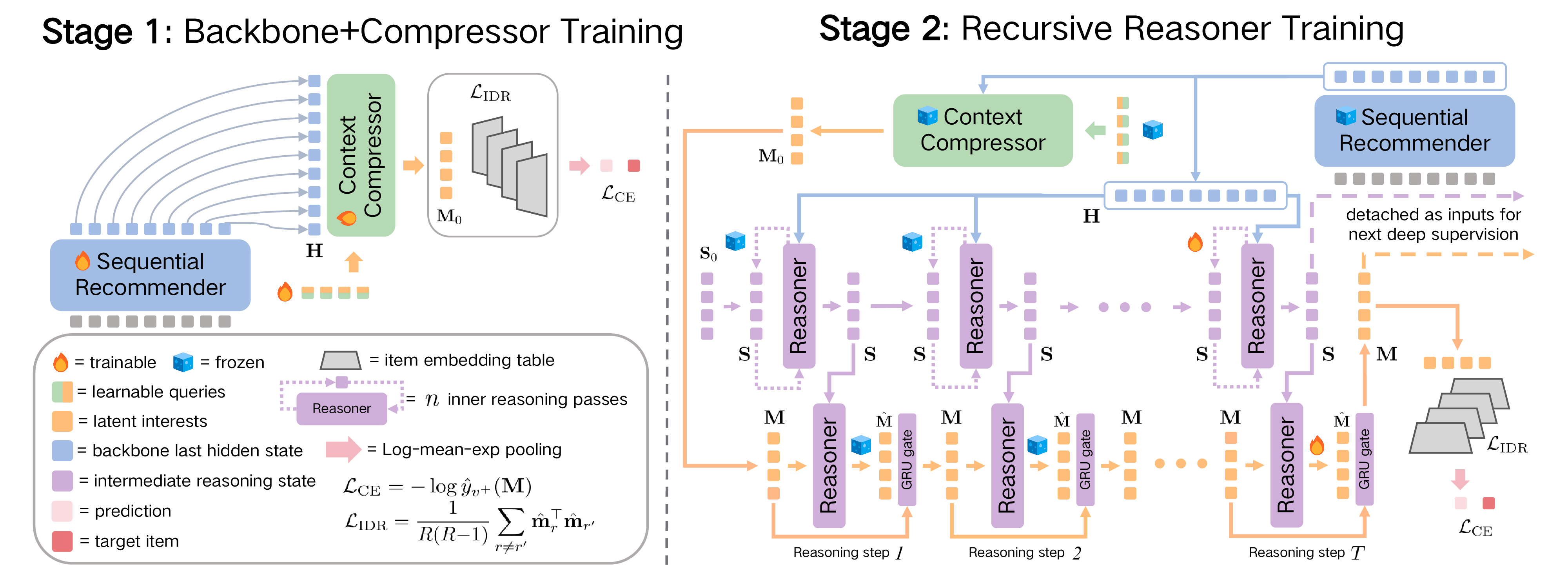
We propose RecRec, a backbone-agnostic framework that introduces the dual-state recursive reasoning paradigm to sequential recommendation. A Context Compressor distills the backbone’s \(L\) hidden states into a small set of \(R\) latent interests. A Recursive Reasoner then alternates between refining an intermediate reasoning state, which revisits the user’s behavior history and the current interests, and committing an update to the interests through a single Transformer block. The framework is trained in two simple supervised stages. Our main contributions are as follows.
We introduce RecRec, to the best of our knowledge the first framework to bring dual-state recursive reasoning to sequential recommendation. Reasoning happens in a dedicated intermediate reasoning state that is separate from the latent interests used for prediction, so intermediate computation does not directly constrain the prediction state, removing the single \(d\)-dimensional bottleneck of prior methods.
A Recursive Reasoner bridges this paradigm to the recommendation setting with a single Transformer block alternating between the two states, where the intermediate reasoning state selectively attends to the user’s behavior history and current interests. This replaces TRM’s concatenation-based MLP with attention-based information routing tailored to the recommendation setting.
A Context Compressor distills the backbone’s hidden states into \(R\) latent interests that jointly produce the prediction. An Interest Diversity Regularizer (IDR) encourages each interest to capture a distinct aspect of user behavior.
Through deep supervision with detached steps and without an RL stage, the reasoning depth can be freely adjusted at inference time beyond the reasoning depth used at training.
Experiments on four real-world datasets show that RecRec outperforms state-of-the-art reasoning-enhanced sequential recommenders. On three of four datasets, gains extend past the training-time depth.
2 Related Work↩︎
2.1 Sequential Recommendation↩︎
Sequential recommendation predicts the next item a user will interact with based on their ordered interaction history. GRU4Rec [16] and Caser [17] first applied recurrent and convolutional architectures to this task. SASRec [18] introduced unidirectional self-attention that lets each position attend to all previous items. BERT4Rec [19] adopted bidirectional self-attention with a cloze-style masked item prediction objective, allowing each position to leverage both past and future context during training. These Transformer-based models have become the de facto backbone for sequential recommendation, with later variants further incorporating modality features [20]–[30]. Despite architectural differences, all of the above models share one property: they produce a single user representation from one forward pass through, and the prediction is read directly from this representation. There is no mechanism to revisit or refine the user representation before prediction.
Several orthogonal lines of work relax this single-vector design: multi-interest recommenders replace the user vector with a set of interest vectors [31]–[33], LLM-based methods cast recommendation as language modeling or align LLMs with backbones [34]–[37], and generative retrieval replaces dense scoring with semantic-ID autoregression [38], [39].
2.2 Reasoning-Enhanced Sequential Recommendation↩︎
Recent work increases inference-time computation for sequential recommendation by introducing multi-step latent reasoning on top of a backbone encoder.
ReaRec [9] was the first to bring latent reasoning into sequential recommendation. It reuses the backbone for several forward passes, feeding the last hidden state back through the same encoder with dedicated reasoning position embeddings. Each step appends reasoning tokens to the input, so the attention cost per step grows as reasoning tokens accumulate. The reasoning position embeddings are allocated for a fixed number of steps, so inference can use fewer steps than training but cannot use more steps than at training. ReaRec trains with either Ensemble Reasoning Learning (ERL), which aggregates reasoning states, or Progressive Reasoning Learning (PRL), which applies per-step supervision with progressively sharpened targets. LARES [10] also reasons over the full sequence, applying a shared core-block \(k\) times, with \(k\) sampled during training, to allow flexible depth at test time. LARES trains in three stages: self-supervised pre-training with trajectory-level and step-level alignment, followed by reinforcement post-training via GRPO using ranking metrics as reward signals.
From an architectural perspective, these two methods represent opposite ends of the evolving state design space. ReaRec evolves a single \(d\)-dimensional vector per step. LARES evolves all \(L\) hidden states at every step through full self-attention, yet only the last position of the final iteration is used for prediction. Both therefore collapse to a single \(d\)-dimensional vector at the prediction step. In both cases the state being refined is also the state from which the prediction is made, with no separate space for intermediate reasoning. RecRec takes a middle ground by compressing the backbone’s output into \(R\) latent interests and reasoning exclusively on them.
Several concurrent efforts scale reasoning along complementary axes. Parallel Latent Reasoning [40] scales reasoning width via aggregated parallel streams within a single-state paradigm, complementary to our depth-extrapolation axis. Diffusion-based two-stage refinement [41], manifold-constrained adaptive test-time compute [42], and process-reward-guided beam search in generative retrieval [43] explore further orthogonal directions. Prompt-level reflection frameworks over LLM backbones [44] operate in a different paradigm from latent-space reasoning. Across these directions, RecRec’s reason-then-update loop, inspired by TRM [15] (discussed next), is distinguished by maintaining a dedicated intermediate reasoning state separate from the evolving interests.
2.3 Recursive Reasoning Models↩︎
Chain-of-thought prompting [2] demonstrated that multi-step reasoning substantially improves LLM performance on tasks requiring compositional logic, and recent reasoning-focused models [45] have scaled this idea with RL. A parallel line of work replaces discrete token generation with continuous latent reasoning: Coconut [7] trains LLMs to reason entirely in continuous hidden states without emitting intermediate tokens, and recurrent-depth models [8] apply depth-wise recursion in latent space to scale test-time computation. The Universal Transformer [46] earlier showed that iteratively applying the same Transformer block improves compositional generalization. Generating explicit reasoning tokens is expensive and bottlenecked by the vocabulary; latent reasoning can iterate freely in a continuous representation space.
The Hierarchical Reasoning Model (HRM) [14] introduced a two-module recurrent architecture where a high-level module maintains a slow planning state and a low-level module handles rapid step-by-step computation. Building on HRM, TRM [15] unifies both modules into a single shared-weight block that alternates between two roles. An answer state \(y\) maps to the predicted output, while a scratchpad state \(z\) holds intermediate reasoning but is never decoded. Within each round the block is applied \(n\) times to update \(z\), then once to update \(y\). Training uses \(T{-}1\) no-gradient warmup rounds followed by one back-propagated round (1-step BPTT), repeated across \(K\) detached deep supervision steps so each step independently learns to improve whatever input it receives. Because a single block handles all computation, TRM achieves strong results on combinatorially hard tasks such as Sudoku and ARC-AGI.
RecRec introduces recursive reasoning to sequential recommendation. The latent interests \(\mathbf{M}\) correspond to TRM’s answer state \(y\), and the intermediate reasoning state \(\mathbf{S}\) to the scratchpad \(z\).
3 Method↩︎
RecRec is designed to work with any sequential backbone. Figure 1 illustrates the overall architecture. Given a sequential backbone, a Context Compressor (§3.2) first extracts the last layer’s hidden states into a compact array of \(R\) latent interests via learned queries and cross-attention. A Recursive Reasoner (§3.3) then iteratively refines these interests through a reason-then-update loop. The refined interests directly predict item relevance via log-mean-exp pooling (§3.4). The framework is trained in two supervised stages (§3.5).
3.1 Problem Formulation↩︎
In sequential recommendation, each user is associated with a chronologically ordered interaction sequence \(\mathbf{x} = (v_1, v_2, \ldots, v_L)\) where \(v_i \in \mathcal{V}\) denotes an item from the item set. The task is to predict the next item \(v_{L+1}\) the user is likely to interact with.
A sequential backbone (e.g., SASRec [18] or BERT4Rec [19]) encodes the interaction sequence and produces hidden states \(\mathbf{H} \in \mathbb{R}^{L \times d}\), where \(L\) is the sequence length and \(d\) is the hidden dimension. Standard practice predicts from only the final position’s hidden state \(\mathbf{h}_L\), compressing the entire interaction history into a single \(d\)-dimensional vector.
RecRec augments this pipeline by extracting \(R\) latent interests from \(\mathbf{H}\), iteratively refining them through recursive reasoning, and predicting items directly from the refined interests. Given the user’s behavior history \(\mathbf{H}\) and an initial estimate of their interests, the question RecRec asks at each reasoning step (formally defined in §3.3) is: with what is known now, how can these interests be revised to better anticipate what the user wants next?
3.2 Context Compressor↩︎
The Context Compressor extracts the backbone’s last-layer hidden states \(\mathbf{H} \in \mathbb{R}^{L \times d}\) into a compact array of \(R\) latent interests \(\mathbf{M}_0 \in \mathbb{R}^{R \times d}\), reducing a variable-length interaction history to a fixed-size representation for the downstream Recursive Reasoner to refine. The compressor uses \(R\) learned queries that cross-attend to the input sequence and are refined through cross-attention layers, following the learned-query cross-attention design [47], [48].
The input sequence is first normalized once: \(\bar{\mathbf{H}} = \mathrm{LN}_{\text{input}}(\mathbf{H})\), and this normalized representation is shared across all layers. The learned queries are initialized with Xavier uniform and expanded to the batch dimension; no positional encoding is applied, as the \(R\) latent interests form an unordered set.
Let \(\mathbf{Z}\) denote the queries being refined, initialized to the learned queries. Each layer applies three pre-norm residual sub-operations: \[\begin{align} \mathbf{Z} &\leftarrow \mathbf{Z} + \mathrm{CrossAttn}\!\bigl( \mathrm{LN}_{\text{crossattn}}(\mathbf{Z}),\; \bar{\mathbf{H}},\; \bar{\mathbf{H}} \bigr), \tag{1} \\[3pt] \mathbf{Z} &\leftarrow \mathbf{Z} + \mathrm{SelfAttn}\!\bigl( \mathrm{LN}_{\text{selfattn}}(\mathbf{Z}) \bigr), \tag{2} \\[3pt] \mathbf{M}_0 &= \mathbf{Z} + \mathrm{FFN}\!\bigl( \mathrm{LN}_{\text{ffn}}(\mathbf{Z}) \bigr). \tag{3} \end{align}\] In the cross-attention, normalization is applied to the queries; \(\bar{\mathbf{H}}\) reuses the input normalization. Padding positions in \(\bar{\mathbf{H}}\) are masked via a key padding mask. Neither cross-attention nor self-attention uses a causal mask, as the \(R\) latent interests form an unordered set.
3.3 Recursive Reasoner↩︎

The Recursive Reasoner iteratively refines the latent interests \(\mathbf{M}_0\) produced by the Context Compressor. To decouple the roles of reasoning and prediction, we maintain two separate states. Latent interests \(\mathbf{M} \in \mathbb{R}^{R \times d}\) are the representations decoded into predictions; they are initialized from \(\mathbf{M}_0\). An intermediate reasoning state \(\mathbf{S} \in \mathbb{R}^{R \times d}\) carries out intermediate reasoning but is never directly used for prediction. We match \(\mathbf{S}\) to \(\mathbf{M}\)’s shape so that a single shared Reasoner block (introduced below) processes both with the same query dimension. A reasoning step consists of \(n\) inner passes in which \(\mathbf{S}\) gathers information from \(\mathbf{H}\) and the current \(\mathbf{M}\), followed by one gated update that commits this information back to \(\mathbf{M}\) through a GRU [49] gate. At the start of each supervision round, \(\mathbf{S}\) is initialized from a fixed random tensor \(\mathbf{S}_0 \in \mathbb{R}^{R \times d}\), drawn once at model construction from a truncated normal distribution. We keep \(\mathbf{S}_0\) fixed rather than learnable because the first \(T{-}1\) reasoning steps of every supervision round run without gradient (see below), so a learnable \(\mathbf{S}_0\) would never receive a gradient signal to update. This separation of roles lets the model reason deeply through \(\mathbf{S}\) without destabilizing \(\mathbf{M}\). In particular, since \(\mathbf{S}\) is never used for prediction, its representations can evolve at a different magnitude from the latent interests, which must stay compatible with the item embeddings used to predict the relevance (via dot product, see §3.4). The GRU gate on \(\mathbf{M}\) further controls how much of this freely evolved reasoning is committed to the prediction state at each step. A single Transformer block handles both roles, updating \(\mathbf{S}\) and \(\mathbf{M}\) with the same parameters but different inputs. The two-state formulation follows recursive reasoning models [15].
3.3.0.1 The Reasoner block.
Both states are updated by a single Transformer [50] block, denoted as \(\mathrm{Reasoner}(\cdot,\cdot)\) in the equations below, with pre-norm LayerNorm, bias-free multi-head attention, and a SwiGLU [51] feed-forward network. Queries and key-value inputs are normalized by separate LayerNorm layers, matching the normalization structure of the Context Compressor. When additional KV tokens \(\mathbf{C}\) are provided, they are normalized by a separate KV norm and appended to the key-value set: \[\begin{align} \mathbf{X}' &= \mathbf{X} + \mathrm{Attn}\!\bigl( \mathrm{LN}_q(\mathbf{X}),\; [\mathrm{LN}_q(\mathbf{X});\, \mathrm{LN}_{kv}(\mathbf{C})] \bigr), \tag{4} \\ \mathrm{Reasoner}(\mathbf{X}, \mathbf{C}) &= \mathbf{X}' + \mathrm{FFN}\!\bigl(\mathrm{LN}_{\text{ffn}}(\mathbf{X}')\bigr), \tag{5} \end{align}\] where \(\mathrm{LN}_q\), \(\mathrm{LN}_{kv}\), and \(\mathrm{LN}_{\text{ffn}}\) are separate LayerNorm layers. Both the attention output projection and the FFN output layer are zero-initialized, so the Reasoner starts as an identity mapping. This stabilizes early training by letting the Reasoner learn to modify the representations it receives from the Context Compressor.
3.3.0.2 The reasoning step.
Each reasoning step proceeds in two phases. First, the intermediate reasoning state is updated for \(n\) inner reasoning passes, each time attending to the full backbone hidden states \(\mathbf{H}\) and the current latent interests: \[\mathbf{S} \leftarrow \mathrm{Reasoner}\bigl(\mathbf{S},\; [\mathbf{H};\, \mathbf{M}]\bigr), \quad \text{repeated } n \text{ times}, \label{eq:s95update}\tag{6}\] where \(\mathbf{H} \in \mathbb{R}^{L \times d}\) is the sequence of hidden states from the frozen backbone. Padding positions in \(\mathbf{H}\) are masked in the key-value attention; \(\mathbf{M}\) is held fixed while \(\mathbf{S}\) evolves, so each pass lets \(\mathbf{S}\) re-examine the encoded user history in light of the current interests.
Second, \(\mathbf{M}\) reads the refined intermediate reasoning state through the Reasoner block, producing a candidate update \(\hat{\mathbf{M}}\) that a GRU gate then blends into the committed \(\mathbf{M}\): \[\begin{align} \hat{\mathbf{M}} &= \mathrm{Reasoner}(\mathbf{M},\; \mathbf{S}), \tag{7} \\ \mathbf{M} &\leftarrow \mathrm{GRU}(\hat{\mathbf{M}},\; \mathbf{M}_{\mathrm{prev}}), \tag{8} \end{align}\] where \(\mathbf{M}_{\mathrm{prev}}\) is the value of \(\mathbf{M}\) before the current reasoning step. Directly overwriting \(\mathbf{M}\) with \(\hat{\mathbf{M}}\) risks large jumps per reasoning step. Following Slot Attention [52], we apply a GRU [49] gate that blends \(\hat{\mathbf{M}}\) with \(\mathbf{M}_{\mathrm{prev}}\), letting the model learn how much to change at each step. The gate’s inputs are layer-normalized before the blending ratio is computed, so the update decision is not affected by representation magnitude.
3.3.0.3 Deep supervision and reasoning depth.
Rather than training the Reasoner with a single loss at the end of all reasoning, we adopt deep supervision [14]: a loss is computed after each of \(K\) supervision rounds, with \(\mathbf{S}\) and \(\mathbf{M}\) detached between rounds. This detachment forces each round to improve whatever state it receives, rather than co-adapting with earlier rounds through long gradient chains: each round learns the same “given state, make it better” objective independently. Each supervision round executes \(T\) reasoning steps, of which only the final step is back-propagated through; the first \(T{-}1\) steps execute without gradient, preparing a good starting point for \(\mathbf{M}\) without consuming gradient memory (a 1-step back-propagation-through-time (BPTT) strategy, following [15]). The total training reasoning depth is therefore \(K \times T\) steps, each containing \(n\) inner reasoning passes. Because each round operates on its inputs independently with no dependence on the history of preceding rounds, the Reasoner can be applied for additional steps beyond the training configuration at inference, deepening the refinement of the latent interests before prediction.
3.4 Prediction↩︎
After reasoning, the refined latent interests \(\mathbf{M}_K \in \mathbb{R}^{R \times d}\) are used to predict the relevance of all candidate items. Each latent interest computes a per-item relevance via inner product with the item embedding \(\mathbf{e}_v \in \mathbb{R}^d\) from the shared embedding table, scaled by a temperature \(\tau\): \[s_r(v) = \frac{\mathbf{m}_r^\top \mathbf{e}_v}{\tau}, \quad r = 1, \ldots, R. \label{eq:per95interest95score}\tag{9}\] The \(R\) per-interest relevances are aggregated into a single prediction \(s(v)\). We want the most relevant interest to dominate the prediction, while keeping gradients flowing through all \(R\) interests so that every interest can be refined during training. A log-mean-exp pooling provides this soft maximum behavior: \[s(v) = \log \frac{1}{R} \sum_{r=1}^{R} \exp\bigl(s_r(v)\bigr). \label{eq:lse95pool}\tag{10}\] This serves as the final prediction for both training and evaluation.
3.5 Training and Inference↩︎
RecRec is trained in two supervised stages.
3.5.0.1 Stage 1: Backbone and compressor co-training.
The backbone and Context Compressor are jointly trained from scratch. The backbone encodes the interaction sequence into \(\mathbf{H}\), and the Context Compressor produces initial latent interests \(\mathbf{M}_0\). The Recursive Reasoner is not used in this stage; item relevance is predicted directly from \(\mathbf{M}_0\) via log-mean-exp pooling (Eq. 10 ) and supervised with cross-entropy loss against the ground-truth next item \(v^+\). An interest diversity regularizer \(\mathcal{L}_{\text{IDR}}\) is added to prevent the learned queries from collapsing to identical interests. The softmax probability of the ground-truth item under the scores \(s(\cdot)\) (Eq. 10 ) computed from a given interest tensor is: \[\hat{y}_{v^+}(\mathbf{M}) = \frac{\exp\bigl(s(v^+)\bigr)}{\sum_{v \in \mathcal{V}} \exp\bigl(s(v)\bigr)}, \label{eq:softmax95prob}\tag{11}\] where the scores \(s(v)\) are obtained from \(\mathbf{M}\) via Eq. 9 and Eq. 10 . The Stage 1 loss is: \[\mathcal{L}_1 = -\log \hat{y}_{v^+}(\mathbf{M}_0) + \lambda_{\text{IDR}} \cdot \mathcal{L}_{\text{IDR}}. \label{eq:loss95s1}\tag{12}\]
3.5.0.2 Interest diversity regularization (IDR)
All \(R\) learned queries attend to the same hidden states \(\mathbf{H}\) via cross-attention. Without explicit regularization, they converge to attend to the same region of the sequence, producing near-identical latent interests (inter-interest cosine similarity exceeds \(0.8\) in practice). IDR penalizes this collapse by minimizing the mean off-diagonal cosine similarity among \(\mathbf{M}_0\)’s interests: \[\mathcal{L}_{\text{IDR}} = \frac{1}{R(R{-}1)} \sum_{r \neq r'} \hat{\mathbf{m}}_r^\top \hat{\mathbf{m}}_{r'}, \label{eq:idr95loss}\tag{13}\] where \(\hat{\mathbf{m}}_r = \mathbf{m}_r / \lVert \mathbf{m}_r \rVert\) denotes the L2-normalized interest. With IDR active, inter-interest cosine drops from \(0.82\)–\(0.90\) to \(0.14\)–\(0.75\) across datasets (see Figure 5), maintaining sufficient diversity for the downstream prediction to benefit from distinct interests.
3.5.0.3 Stage 2: Recursive Reasoner training.
The backbone is frozen (eval mode). The Context Compressor is also frozen but keeps dropout active, serving as a regularizer on the Reasoner’s input. The Recursive Reasoner is initialized from scratch and is the only trainable component, zero-initialized so that it starts as an identity mapping, stabilizing early training.
Training follows the deep supervision scheme of §3.3 with \(K\) supervision rounds per batch. At each round \(k\): the Reasoner takes \(\mathbf{H}\) and the detached \(\mathbf{S}\), \(\mathbf{M}\) from the previous round and runs \(T\) reasoning steps; only the final step, consisting of \(n\) inner reasoning passes on \(\mathbf{S}\) and one gated update on \(\mathbf{M}\), is back-propagated through (1-step BPTT); the loss in Eq. 14 is computed on the resulting \(\mathbf{M}^{(k)}\), one gradient step is taken, and both \(\mathbf{S}^{(k)}\) and \(\mathbf{M}^{(k)}\) are detached before being fed to round \(k{+}1\). At the first round, \(\mathbf{S}\) is initialized from \(\mathbf{S}_0\) and \(\mathbf{M}\) from \(\mathbf{M}_0\). The Stage 2 loss at round \(k\) adds IDR to the cross-entropy on \(\mathbf{M}^{(k)}\): \[\mathcal{L}_2^{(k)} = -\log \hat{y}_{v^+}(\mathbf{M}^{(k)}) + \lambda_{\text{IDR}} \cdot \mathcal{L}_{\text{IDR}}(\mathbf{M}^{(k)}), \quad k = 1, \ldots, K. \label{eq:loss95s2}\tag{14}\]
3.5.0.4 Inference.
Figure 2 summarizes the Reasoner block and its outer loop at inference. At inference, the Reasoner is applied for \(N\) reasoning steps, each consisting of \(n\) inner passes on \(\mathbf{S}\) and one gated update to \(\mathbf{M}\). At training, \(N = K \times T\) is determined by the deep supervision schedule (Eq. 14 ); at inference, there is no supervision, so \(N\) can be chosen freely. Because the Reasoner learns to improve whatever state it receives, the model can be evaluated at values of \(N\) larger than used during training, without retraining.
4 Experiments↩︎
| Dataset | #Users | #Items | #Inter. | Avg.L | Sparsity |
|---|---|---|---|---|---|
| S-Shop | 89,284 | 15,552 | 384,741 | 12.64 | 99.97% |
| V-Shop | 54,005 | 21,439 | 249,505 | 14.77 | 99.98% |
| MicroLens | 98,133 | 16,959 | 502,561 | 5.12 | 99.97% |
| Steam | 157,998 | 7,960 | 1,292,442 | 25.97 | 99.90% |
We organize the experimental evaluation around three research questions: RQ1: Does RecRec’s dual-state design outperform prior reasoning-enhanced methods? RQ2: Does deep supervision enable flexible reasoning depth at inference, including beyond the training-time depth? RQ3: How do the latent interests and other components of RecRec contribute to its overall performance?
4.1 Experimental Setup↩︎
4.1.1 Datasets.↩︎
We conduct experiments on four datasets: two shopping datasets [53], a short-video dataset (MicroLens [54]), and a gaming dataset (Steam [18]), all filtered with a 5-core threshold. For simplicity, we refer to the two shopping datasets as S-Shop and V-Shop. To ensure training quality, we further remove users whose training split contains fewer than 5 interactions. Statistics are in Table 2.
S-Shop and V-Shop. The two shopping datasets contain product ratings and reviews: S-Shop covers user interactions with software products, while V-Shop covers user interactions with video games. Together they span e-commerce scenarios of different scales and sparsity levels. To focus on positive interaction signals, we retain only records with ratings above 3. Interaction sequences are constructed by sorting records by timestamp. Since both datasets provide absolute timestamps, the training, validation, and test splits follow the official temporal partitions.
MicroLens-100K. MicroLens-100K is a short-video recommendation dataset that records user click behavior on a short-video platform. Unlike the e-commerce datasets, it contains only implicit feedback (clicks), making the interaction patterns closer to real-world feed recommendation scenarios. The raw data is provided as time-ordered user interaction sequences without absolute timestamps. We adopt a relative time split at the 80% and 90% positions of each user’s sequence length for training, validation, and test sets.
Steam. The Steam dataset is collected from user reviews on the Steam gaming platform and serves as a classic benchmark in sequential recommendation, widely adopted by representative methods such as SASRec and BERT4Rec. Since the raw data may contain multiple reviews from the same user for the same game, we deduplicate and keep only the first review. As with MicroLens, the dataset lacks absolute timestamps, so we adopt a relative time split at the 80% and 90% positions of each user’s interaction sequence.
4.1.2 Baselines.↩︎
We compare RecRec against two groups of baselines. Non-reasoning methods. SASRec [18] uses causal self-attention to encode user interaction sequences. BERT4Rec [19] applies bidirectional self-attention with masked item prediction.
Reasoning-enhanced methods. ERL and PRL [9] are two variants of ReaRec that perform multi-step reasoning by autoregressively feeding the last hidden state back into the backbone encoder. ERL aggregates reasoning states via ensemble, while PRL uses progressive contrastive learning. Both are evaluated with SASRec (S) and BERT4Rec (B) backbones. LARES [10] is a depth-recurrent reasoning model that iterates a shared core-block over the full token sequence, trained with self-supervised pre-training and reinforcement post-training. ERL and PRL results come from the official ReaRec codebase; LARES from its official implementation.
4.1.3 Implementation Details.↩︎
We report NDCG@\(K\) and Recall@\(K\) for cutoffs 10 and 20, evaluated under full ranking. To ensure fair comparison, all baselines use an embedding dimension of 256, a batch size of 2048, the AdamW optimizer at a learning rate of \(10^{-3}\), early stopping with patience 10 on validation NDCG@10, and a temperature \(\tau = 0.07\) across all experiments.
For RecRec Stage 1, the Context Compressor uses \(R = 8\) latent interests, 1 layer, and 2 attention heads, with an FFN inner dimension of 512. \(\lambda_{\text{IDR}}\) is tuned from \(\{0, 0.01, 0.05, 0.1\}\). For Stage 2, the reasoning configuration is \(T = 3\) reasoning steps per supervision round, \(K = 3\) supervision rounds, and \(n = 3\) inner reasoning passes, giving \(N = K \times T = 9\) reasoning steps at training. The Reasoner uses 1 layer, 2 attention heads, and an FFN inner dimension of 512.
4.2 Overall Performance (RQ1)↩︎
cl ccccccc >cc >cc & & & &
(lr)3-4 (lr)5-9 (lr)10-11 Dataset & Metric & BERT4Rec & SASRec & ERL (B) & ERL (S) & PRL (B) & PRL (S) & LARES & RecRec (B) & RecRec (S)
& N@10 & 0.0734 & 0.0737 & 0.0766 & 0.0776 & 0.0777 & 0.0818 & 0.0809 & 0.0833 & 0.0853\(^\ast\)
& N@20 & 0.0950 & 0.0952 & 0.0982 & 0.0989 & 0.0997 & 0.1015 & 0.1009 & 0.1039 & 0.1058\(^\ast\)
& R@10 & 0.1570 & 0.1544 & 0.1594 & 0.1616 & 0.1627 & 0.1568 & 0.1530 & 0.1638 & 0.1619
& R@20 & 0.2426 & 0.2399 & 0.2450 & 0.2461 & 0.2461 & 0.2351 & 0.2328 & 0.2501 & 0.2432
& N@10 & 0.0153 & 0.0158 & 0.0160 & 0.0161 & 0.0155 & 0.0173 & 0.0182 & 0.0184 & 0.0197\(^\ast\)
& N@20 & 0.0196 & 0.0206 & 0.0204 & 0.0217 & 0.0215 & 0.0221 & 0.0222 & 0.0241 & 0.0248\(^\ast\)
& R@10 & 0.0303 & 0.0289 & 0.0324 & 0.0378 & 0.0348 & 0.0381 & 0.0327 & 0.0422 & 0.0449\(^\ast\)
& R@20 & 0.0476 & 0.0479 & 0.0500 & 0.0601 & 0.0586 & 0.0571 & 0.0488 & 0.0649 & 0.0651\(^\ast\)
& N@10 & 0.0428 & 0.0428 & 0.0435 & 0.0432 & 0.0448 & 0.0453 & 0.0460 & 0.0481 & 0.0503\(^\ast\)
& N@20 & 0.0523 & 0.0533 & 0.0533 & 0.0538 & 0.0554 & 0.0562 & 0.0564 & 0.0585 & 0.0611\(^\ast\)
& R@10 & 0.0885 & 0.0875 & 0.0865 & 0.0893 & 0.0898 & 0.0908 & 0.0863 & 0.0921 & 0.0939
& R@20 & 0.1263 & 0.1291 & 0.1251 & 0.1313 & 0.1318 & 0.1344 & 0.1276 & 0.1331 & 0.1370
& N@10 & 0.0343 & 0.0347 & 0.0371 & 0.0383 & 0.0385 & 0.0408 & 0.0419 & 0.0477 & 0.0481\(^\ast\)
& N@20 & 0.0459 & 0.0454 & 0.0496 & 0.0505 & 0.0501 & 0.0535 & 0.0545 & 0.0607 & 0.0621\(^\ast\)
& R@10 & 0.0695 & 0.0698 & 0.0723 & 0.0780 & 0.0754 & 0.0804 & 0.0831 & 0.0922 & 0.0978\(^\ast\)
& R@20 & 0.1158 & 0.1126 & 0.1219 & 0.1266 & 0.1214 & 0.1308 & 0.1330 & 0.1440 & 0.1536\(^\ast\)
Table ¿tbl:tab:main95results? presents the overall results. For a fair comparison with baselines whose reasoning depth is fixed at training, we report RecRec’s prediction at \(N = 9\), without selecting the inference-time peak; Section 4.3 examines those sweeps. RecRec variants achieve the best performance on all four datasets. RecRec (S) improves NDCG@10 over the best reasoning-enhanced baseline by 14.8% on Steam, 9.3% on MicroLens, 8.2% on V-Shop, and 4.3% on S-Shop. These gains come against baselines that either entangle the reasoning state with the input sequence or derive predictions from a single \(d\)-dim vector, both limitations that RecRec removes by design. RecRec (S) generally outperforms RecRec (B), opposite to what one might expect from BERT4Rec’s bidirectional context. NDCG gains match or exceed Recall gains across datasets, indicating that recursive reasoning helps rank the target item higher rather than merely expanding the recall set.
Answer to RQ1: RecRec’s dual-state design outperforms all reasoning-enhanced baselines across four datasets. These baselines either entangle reasoning with the input sequence or predict from a single vector; decoupling reasoning from prediction and using multiple latent interests both contribute to this lift.
4.3 Inference-Time Reasoning Depth (RQ2)↩︎

Figure 3 reports NDCG@20 as the inference-time \(N\) varies from \(0\) to \(16\). Two patterns stand out across datasets. Moving from \(N = 0\) (the Stage-1 baseline) to \(N = 1\) produces a large jump in NDCG, for example from \(0.0966\) to \(0.103\) on S-Shop (SASRec) and from \(0.0496\) to \(0.058\) on Steam (SASRec). The first Reasoner pass alone therefore accounts for a large share of the gain over the Stage-1 baseline. Additional reasoning steps continue to refine the state, with diminishing returns. The Reasoner improves a rough starting state substantially within a few passes, while refinement of an already-improved state produces smaller gains.
Increasing \(N\) beyond \(9\) continues to yield small additional improvements on S-Shop, V-Shop, and Steam, where the best-performing \(N\) lies at \(15\), \(12\), and \(16\) respectively (e.g., from \(0.1058\) to \(0.1062\) on S-Shop (SASRec); from \(0.0248\) to \(0.0251\) on V-Shop (SASRec)). The model remains stable when \(N\) is pushed well beyond \(9\). On MicroLens, the initial Reasoner pass also produces a clear improvement, but the gains are smaller, and the curve saturates near \(N \approx 4\) and then declines.
Answer to RQ2: Deep supervision enables RecRec to use flexible reasoning depth at inference. The largest gain comes from the first few steps, and on three of four datasets, performance is sustained past the training-time depth \(N = 9\) with small additional gains. This extrapolation is what deep supervision with detached steps sets up. Each round is trained to improve whatever state it receives, so the Reasoner can keep doing this when more steps are appended.
4.4 Ablation Study (RQ3)↩︎
Figure 4 reports the ablation study on RecRec components on S-Shop and Steam with the SASRec backbone. We evaluate four variants against the full RecRec and the raw SASRec backbone as a non-reasoning reference. w/o Reasoner predicts directly from \(\mathbf{M}_0\), skipping Stage-2 entirely and testing the Reasoner’s overall contribution. Frozen \(\mathbf{S}\) (\(n{=}0\)) keeps \(\mathbf{S}\) fixed at \(\mathbf{S}_0\), isolating the iterative refinement of the intermediate reasoning state. w/o GRU gate replaces the gated \(\mathbf{M}\) update with direct overwriting. w/o IDR removes the diversity regularizer from both training stages. All variants are evaluated at \(N = 9\).
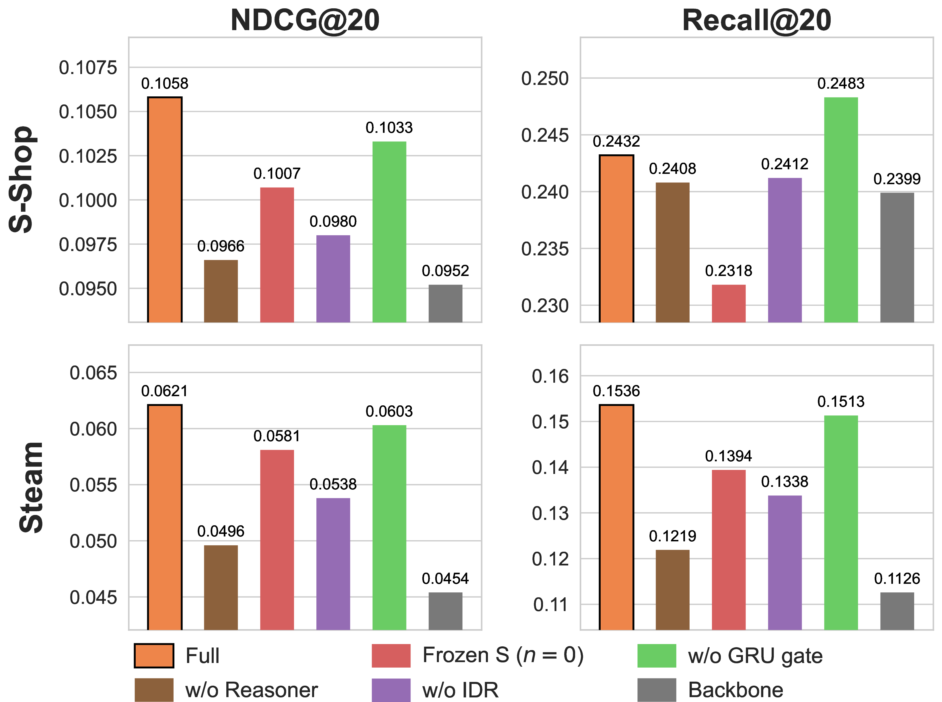
On both datasets, NDCG@20 follows the same pattern, with the raw SASRec backbone trailing all variants. The full RecRec leads, and removing the Reasoner or IDR drops to roughly the Stage-1 baseline level while removing the GRU gate or fixing \(\mathbf{S}\) at \(\mathbf{S}_0\) causes moderate drops in between. Removing the Reasoner equals the Stage-1 baseline by construction. Removing IDR drops to a similar level: with the diversity regularizer disabled in both training stages, the \(R\) latent interests collapse to near-identical directions in the final \(\mathbf{M}\) (verified in Figure 5). Fixing \(\mathbf{S}\) at \(\mathbf{S}_0\) (zero inner reasoning passes) lowers NDCG on both datasets, degenerating the dual-state design into \(\mathbf{M}\)-only evolution where the intermediate reasoning state contributes nothing \(\mathbf{M}\) does not already carry. Removing the GRU gate also costs NDCG, but less than fixing \(\mathbf{S}\); the gate shapes how each candidate update is absorbed into \(\mathbf{M}\) rather than whether the update mechanism works. The Recall@20 ordering largely follows NDCG@20 with one exception. On S-Shop, removing the gated update slightly exceeds full RecRec (\(0.2483\) vs.\(0.2432\)), suggesting that the gate trades a small amount of Recall coverage for sharper ranking.
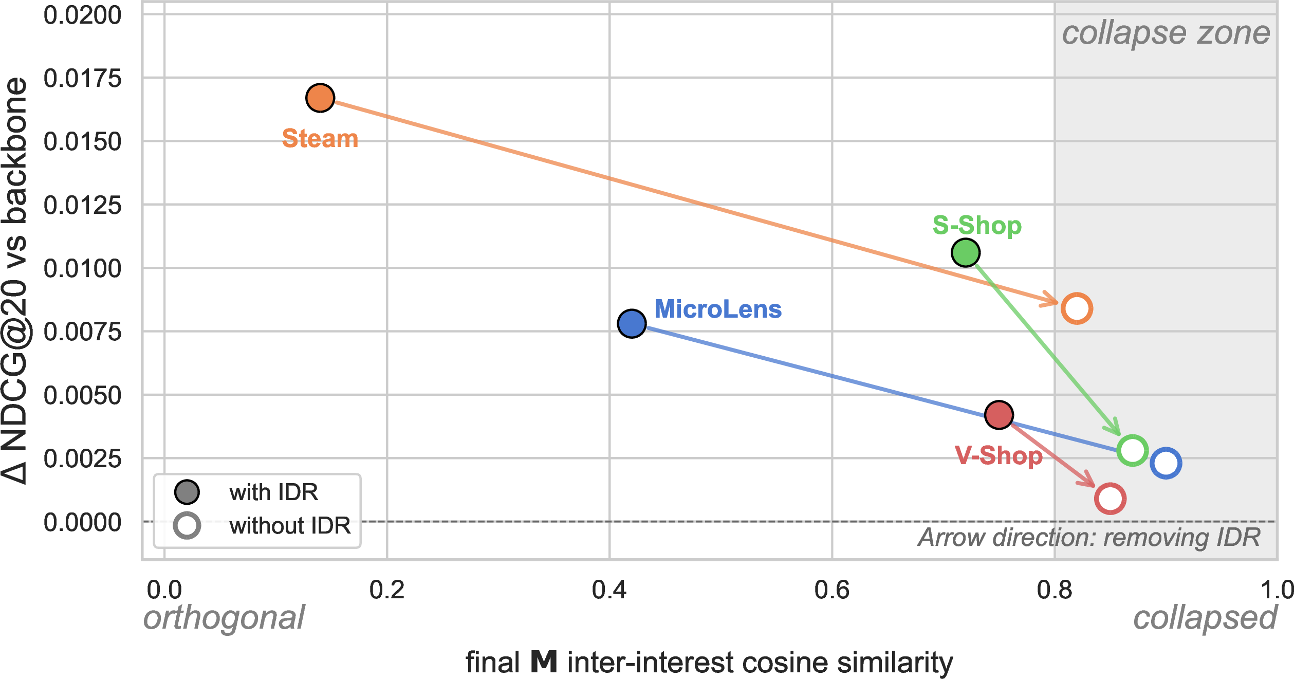
Figure 5 measures the inter-interest cosine similarity of the final latent interests \(\mathbf{M}\) on the test set. Without IDR, \(\mathbf{M}\)’s \(R\) interests collapse to nearly identical directions across all four datasets, falling into the marked collapse zone. With IDR, the interests stay diverse to varying degrees across datasets. The NDCG@20 improvement gained by enabling IDR (the vertical drop of each arrow) tracks the cosine reduction. IDR keeps the \(R\) interests separable, and the Reasoner’s gain depends on having distinct interests to refine.
4.4.0.1 R sweep.
Table 3 reports the \(R\) sweep on NDCG@20, with \(R\) kept consistent between Stage 1 and Stage 2. A single-vector latent (\(R{=}1\)) trails every multi-vector configuration on every dataset, the clearest signal that the prediction state benefits from carrying more than a single \(d\)-dimensional vector. Beyond \(R{=}2\) the optimum is dataset-dependent without a single explanatory axis. \(R{=}4\) wins on V-Shop and MicroLens, \(R{=}8\) on Steam, \(R{=}16\) on S-Shop. Pushing to \(R{=}16\) degrades performance on V-Shop and MicroLens, suggesting that an overly large \(R\) can dilute the training signal across slots that the dataset cannot fully populate. The default \(R{=}8\) stays within \(5\%\) of the per-dataset best, a safe middle-ground choice.
| \(R\) | 1 | 2 | 4 | 8 | 16 |
|---|---|---|---|---|---|
| S-Shop | 0.0990 | 0.1001 | 0.1078 | 0.1058 | 0.1095 |
| V-Shop | 0.0219 | 0.0237 | 0.0255 | 0.0248 | 0.0239 |
| MicroLens | 0.0554 | 0.0614 | 0.0618 | 0.0611 | 0.0587 |
| Steam | 0.0520 | 0.0567 | 0.0604 | 0.0621 | 0.0618 |
Answer to RQ3: Every component of RecRec contributes. The Reasoner, IDR, and \(n\) inner reasoning passes that evolve \(\mathbf{S}\) are required for the dual-state design to deliver, while the GRU gate shapes how each update is absorbed into \(\mathbf{M}\) rather than whether the update works. A multi-vector prediction latent (\(R \geq 2\)) outperforms a single vector across four datasets, with the optimal \(R\) dataset-dependent.
5 Conclusion↩︎
We presented RecRec, a recursive reasoning framework for sequential recommendation that separates the reasoning state from the prediction state and predicts from \(R\) latent interests rather than a single vector. A Context Compressor with an Interest Diversity Regularizer initializes the latent interests, and a Recursive Reasoner refines them through alternating updates with a dedicated reasoning state. The framework is trained in two supervised stages, with deep supervision and detached steps allowing inference-time reasoning depth to be adjusted freely. Experiments on four datasets show consistent gains over reasoning-enhanced baselines; on three of four datasets, gains extend past the training-time reasoning depth. Taken together, our results show that the gain from recursive reasoning in sequential recommendation comes primarily from two architectural choices: detaching the reasoning state from the prediction latent, and predicting from a set of latent interests rather than a single vector. Both are lightweight and backbone-agnostic, suggesting that reasoning-state architecture is an orthogonal axis worth exploring alongside backbone improvements.
5.0.0.1 Future directions.
A learned halting mechanism [15] would let RecRec stop reasoning early on easy sequences and continue on harder ones, but designing a halting signal for ranking objectives is non-trivial since there is no single discrete correct answer to supervise against. Allowing asymmetric shapes for the reasoning and prediction states, currently constrained to the same \(R{\times}d\) form, is a natural extension that would let the reasoning state carry more capacity than the prediction state. A more behavioral study of how the latent interests evolve across reasoning steps, including gate dynamics and attention patterns, would clarify the mechanism behind the empirical lift and its variation across datasets.