Efficient Sequential Calibration with \(O(T^{2/3-\epsilon})\) Error Bound
July 14, 2026
Abstract
We study the online binary sequential calibration problem. A recent breakthrough by [1] overcomes the classical \(T^{2/3}\) barrier for calibration error. Building on this result, we present an efficient randomized forecaster that achieves an expected calibration error \(O(T^{2/3-\varepsilon})\) for some constant \(\varepsilon>0\).
Our forecaster combines the SPR-Calibration procedure [1] with an outer Blackwell-style correction layer. The SPR-Calibration procedure controls calibration with respect to a surrogate sequence of conditional-mean estimates, while the correction layer controls the additional error incurred when these surrogates are used to approximate the true outcomes. The analysis decomposes the total calibration error into the surrogate calibration error and the residual discrepancy between the surrogate sequence and the true outcomes. The former is bounded by the SPR-Calibration guarantee in [1], and the latter is controlled using a quadratic potential argument together with the sparsity of the SPR-Calibration forecaster.
1 Introduction↩︎
Calibration captures a basic reliability requirement for probabilistic predictions: when a forecaster repeatedly assigns probability \(p\) to an event, the event should occur on roughly a \(p\)-fraction of those rounds. This notion is important because probability forecasts are often used directly in downstream decisions, such as risk assessment, medical prediction, weather forecasting, and machine-learning systems that report confidence scores [2]–[5]. In these applications, the numerical value of a forecast matters, not only the ranking of alternatives: a prediction of \(0.8\) should be interpretable as an event that happens about \(80\%\) of the time. Sequential calibration studies how to achieve this reliability guarantee when predictions are made online and the data may arrive adaptively or non-stationarily.
In this work, we consider the online sequential calibration problem initiated by [6]. At each round \(t\), a forecaster announces a probability \(p_t\in[0,1]\) for a binary outcome \(y_t\in\{0,1\}\). The standard \(\ell_1\)-calibration error after \(T\) rounds is \[\operatorname{CalErr}_T = \sum_{p\in\mathcal{P}_T} \left| \sum_{t\le T:p_t=p}(p-y_t) \right|,\] where \(\mathcal{P}_T\) is the set of distinct predictions used by the forecaster. Classical algorithms achieve calibration error of order \(T^{2/3}\). One way to obtain this rate is through a discretization and Blackwell-approachability argument [7]: the forecaster restricts predictions to a finite grid of size \(m\), controls the calibration residuals over this grid using an approachability strategy, and balances the approachability term \(O(\sqrt{mT})\) with the discretization term \(O(T/m)\). Optimizing over \(m\) gives \(m\asymp T^{1/3}\), and hence calibration error \(O(T^{2/3})\). This approach is conceptually clean and computationally efficient, but it also highlights the longstanding \(O(T^{2/3})\) barrier.
A recent breakthrough by [1] showed that the classical \(O(T^{2/3})\) upper bound is not intrinsic. They introduced an algorithm, which we refer to as SPR-Calibration, that achieves a calibration error bound of order \(O(T^{2/3-\varepsilon})\) for some constant \(\varepsilon>0\), thereby breaking the \(T^{2/3}\) barrier for the first time.
Despite this breakthrough, obtaining an efficient \(O(T^{2/3-\varepsilon})\) guarantee in the sequential setting is not immediate. The SPR-Calibration algorithm [1] is analyzed through a minimax reduction that allows the proof to work in a full-information model, where the forecaster is given the conditional mean \(e_t=\mathbb{E}[y_t\mid \mathcal{F}_{t-1}]\) at each round. This idea goes back to the minimax proof of calibration [8]: if the forecaster knew the adversary’s mixed strategy, then it could simply predict the induced conditional probability of the next outcome; the minimax theorem then converts this observation into the existence of a randomized forecasting strategy that is calibrated against every adversary. However, this minimax transformation is primarily an existence argument rather than a computationally tractable algorithm.
It then naturally raises the question:
Is there an efficient algorithm with \(O(T^{2/3-\varepsilon})\) calibration error?
In this work, we answer this problem affirmatively.
Theorem 1. There exists a forecaster (see Algorithm 5), such that for any sequence \(\{y_t\}_{t=1}^T\in \{0,1\}^T\), the expected calibration error \(\mathbb{E}[\operatorname{CalErr}_T]\) is bounded by \(O(\log_2(T)\cdot T^{2/3 - \varepsilon_{\mathrm{AB}}/18 })\), where \(\varepsilon_{\mathrm{AB}}>0\) is the same as the constant \(\varepsilon\) in Theorem 1.3 of [1]. Moreover, the computation cost of the algorithm is \(O(T^{7/2}\log_2(T))\).
Our algorithm is based a natural combination of the SPR-Calibration procedure of [1] with an outer Blackwell-style correction layer. At each round \(t\), the algorithm first forms a surrogate estimate \(\widetilde{e}_t\) of the conditional mean and then passes this value to the calibration procedure of [1]. Since calibration is ultimately measured against the realized outcome \(y_t\), using the surrogate \(\widetilde{e}_t\) introduces an additional source of error. To control this error, the algorithm augments the underlying calibration procedure with a Blackwell-style correction layer. The analysis separates the total calibration error into two components: the calibration error with respect to the surrogate sequence \(\{\widetilde{e}_t\}_{t=1}^T\), and the discrepancy between the surrogate means and the realized outcomes. The first component is controlled directly by the guarantee of [1]; the second is bounded using a quadratic potential argument together with the sparsity property of their calibration algorithm.
1.1 Related Works↩︎
1.1.0.1 Calibration and adversarial forecasting.
Calibration has a long history as a criterion for evaluating probabilistic forecasts. [2] emphasized calibration as a basic consistency requirement for subjective probabilities, and [6] initiated the adversarial sequential calibration problem studied in this paper. Their work showed that randomized forecasters can be calibrated against arbitrary binary outcome sequences and gave the classical \(O(T^{2/3})\) calibration-error guarantee. Several subsequent works gave alternative proofs and perspectives on calibration, including the myopic minimax construction [9], the Blackwell-approachability proof [7], the minimax proof [8], and the geometric approachability proof [10].
1.1.0.2 Approachability, regret, and calibration.
Blackwell’s approachability theorem [11] is one of the central tools behind adversarial calibration. In the approachability formulation, calibration residuals are treated as coordinates of a vector-valued payoff, and the forecaster chooses predictions so that the cumulative payoff approaches an appropriate target set. This connection was made explicit by [7] and was further developed through geometric and online-learning viewpoints [10], [12]. Calibration is also closely related to regret minimization: [13] connected calibration and internal regret, and calibrated learning rules are known to lead to correlated equilibrium in repeated games [14]. The broader connections between prediction of individual sequences, regret, and game-theoretic learning are surveyed in [15].
1.1.0.3 Rates for sequential calibration.
The optimal rate of \(\ell_1\)-calibration error has been a central question in sequential calibration. The classical upper bound is \(O(T^{2/3})\), obtained by balancing the discretization error of a finite grid with an approachability-type residual term [6], [12]. For many years, the only general lower bound was the trivial \(\Omega(\sqrt T)\) bound obtained from independent fair coin flips. [16] gave the first super-\(\sqrt T\) lower bound, proving an \(\Omega(T^{0.528})\) lower bound via the sign-preservation game. [1] recently broke the \(T^{2/3}\) upper-bound barrier by introducing sign preservation with reuse (SPR), proving that improved SPR strategies yield calibration error \(O(T^{2/3-\varepsilon})\) for some constant \(\varepsilon>0\). They also improved the lower bound to \(\Omega(T^{0.54389})\), leaving a gap between the known upper and lower exponents.
2 Problem Setting↩︎
We follow the sequential calibration setup of [1]. Fix a time horizon \(T\). At each round \(t\in[T]\), the forecaster outputs a probability prediction \(p_t\in[0,1]\), and the environment outputs an outcome \(y_t\in\{0,1\}\). The prediction \(p_t\) is interpreted as the forecaster’s announced probability that \(y_t=1\).
The adversary may be adaptive, in the sense that its choice at time \(t\) may depend on the past history \[H_t:=\{(p_s,y_s):s<t\},\] but it does not observe the current prediction \(p_t\) before choosing \(y_t\).
Let \(\mathcal{P}_t:=\{p_s:s\le t\}\) denote the set of distinct probability values actually output up to time \(t\). Define \(E_t(p) = \sum_{s\le t:p_s=p}(p-y_s).\) The cumulative \(\ell_1\)-calibration error at time \(t\) is \[\operatorname{CalErr}_t := \sum_{p\in\mathcal{P}_t}|E_t(p)| = \sum_{p\in\mathcal{P}_t} \left| \sum_{s\le t:p_s=p}(p-y_s) \right|.\]
When the forecaster is randomized, all quantities above are random variables. We measure performance by expected calibration error \(\mathbb{E}[\operatorname{CalErr}_T]\), where the expectation is over the forecaster’s internal randomness.
We next recall the sign-preservation with reuse game, abbreviated as SPR, introduced in [1].
Definition 1 (Sign-preservation with reuse). For \(n,s\in\mathbb{N}\), the game \(\operatorname{SPR}(n,s)\) is played between two players, called Player-P and Player-L. The game consists of \(n\) cells, indexed by \([n]=\{1,\ldots,n\}\), all of which are initially empty. The game lasts for at most \(s\) rounds. In each round, the following steps occur:
Player-P may terminate the game. Otherwise, Player-P chooses an empty cell \(j\in[n]\).
After observing \(j\), Player-L may remove any subset of the \(-\) signs in cells strictly to the left of \(j\), and any subset of the \(+\) signs in cells strictly to the right of \(j\).
Player-L then places either a \(+\) sign or a \(-\) sign in cell \(j\).
A cell whose sign has been removed becomes empty and may therefore be chosen again in a later round. Player-P aims to maximize the number of signs remaining on the board at the end of the game, while Player-L aims to minimize this quantity.
3 The SPR-Calibration Algorithm↩︎
In this section, we recall the SPR-Calibration construction of [1] and the properties needed in our analysis.
3.1 Deterministic Implementation of SPR-Calibration↩︎
This subsection specifies the version of SPR-Calibration used by our outer algorithm. For completeness, we present the main algorithm of [1] in Algorithm 1, together with its key subroutines: simulateGame in Algorithm 2, the recursive
\(A\)-procedure in Algorithm 3, and the recursive \(B\)-procedure in Algorithm 4.
The feature needed by Algorithm 5 is a deterministic one-step transition. Given the pre-round state \(S\) (see Definition 2), a round index \(t\), and an input \(z\in[0,1]\), define \[\operatorname{Step}_{\mathrm{SPR}}(S,t,z) = (p,S^+),\] where \(p\) is the forecast returned by one round of SPR-Calibration and \(S^+\) is the resulting state. We fix all loop orders, tie-breaking rules, and boundary conventions below, so this transition is well-defined. We then set \[\begin{align} \operatorname{Predict}_{\mathrm{SPR}}(S,t,z) &:= p,\\ \operatorname{Update}_{\mathrm{SPR}}(S,t,z) &:= S^+. \end{align}\]
3.1.0.1 Scales and SPR instances.
Let \(\tau:=\left\lceil\log_2 T\right\rceil\), and let \(\overline{T}:=2^\tau\). Run the first \(T\) rounds of a subroutine initialized for the padded horizon \(\overline{T}\). Since \(T\le \overline{T}<2T\), this padding changes all asymptotic bounds by at most a constant factor. We assume \(\tau\ge2\); the finitely many smaller horizons can be handled by any fixed forecasting rule. Fix an integer \(1\leq h <\tau\). Define \(\mathcal{I}_h:=\{1,\ldots,\tau-h\}\), \(\mathcal{J}_i:=\{i+1,\ldots,i+h\}\) and \(C_i:=\{1,\ldots,2^i\}.\) For every \(i\in\mathcal{I}_h\), \(j\in\mathcal{J}_i\), and \(\ell\in\{0,1\}\), the subroutine maintains one SPR instance \(G_{i,j,\ell}\) with cell set \(C_i\). The index \(i\) specifies the spatial resolution, \(j\) specifies the time scale, and \(\ell\) separates the even and odd dyadic intervals at resolution \(2^{-(i+1)}\).
3.1.0.2 Cells, intervals, and forecast values.
For \(z\in[0,1]\), let \(m_i(z) := \min\left\{ \left\lfloor 2^{i+1}z\right\rfloor, 2^{i+1}-1 \right\}\), \(\ell_i(z) :=m_i(z)\bmod 2\) and \(c_i(z) :=\frac{m_i(z)-\ell_i(z)}{2}+1.\) We define \[\operatorname{cell}(i,j,z) := \bigl(c_i(z),G_{i,j,\ell_i(z)}\bigr).\] Thus, \(j\) selects the SPR instance at the desired time scale, while \(i\) and \(z\) determine the parity and cell.
For \(c\in C_i\) and \(\ell\in\{0,1\}\), write \(m=2(c-1)+\ell\) and define \[\operatorname{interval}(c,G_{i,j,\ell}) := \begin{cases} \left[\dfrac{m}{2^{i+1}},\dfrac{m+1}{2^{i+1}}\right), &m<2^{i+1}-1,\\[2ex] \left[\dfrac{2^{i+1}-1}{2^{i+1}},1\right], &m=2^{i+1}-1. \end{cases}\] In this way, every \(z\in[0,1]\) is assigned to a unique cell1. For a sign \(\sigma\in\{+,-\}\), define \[\operatorname{prob}(c,\sigma,G_{i,j,\ell}) := \begin{cases} \dfrac{\max\{0,2(c-1)+\ell-1\}}{2^{i+1}}, &\sigma=+,\\[2ex] \dfrac{\min\{2(c-1)+\ell+2,2^{i+1}\}}{2^{i+1}}, &\sigma=-. \end{cases}\]
3.1.0.3 The SPR state.
To formalize the subroutines that we borrow from the SPR-Calibration algorithm of [1], we first give a precise definition of the state of an SPR-Calibration instance.
Definition 2 (SPR state). For each instance \(G=G_{i,j,\ell}\), the subroutine stores \[\begin{array}{ll} \operatorname{bias}_G:C_i\to\mathbb{R}, &\text{the accumulated surrogate bias in each cell},\\ \sigma_G:C_i\to\{+,-,\varnothing\}, &\text{the current \mathrm{\small SPR} sign configuration},\\ \mathsf L_G, &\text{the mutable state of the explicit A/B labeler}. \end{array}\] Initially, we set \(\operatorname{bias}_G(c)=0\) and \(\sigma_G(c)=\varnothing\) for every instance \(G\) and cell \(c\). The labeler state \(\mathsf L_G\) is initialized by \(A_G^{\mathrm{root}} :=A.\operatorname{initialize}(1,2^i,0).\)
Accordingly, a query to calibration cell \(c\) is passed directly to the labeler as query \(c\). The complete state is \[\begin{align} S^{\mathrm{SPR}}_{\mathrm{local}} = \left\{ \operatorname{bias}_{G}, \sigma_{G}, \mathsf L_{G} \right\}_{ i\in\mathcal{I}_h, j\in\mathcal{J}_i, \ell\in\{0,1\} }.\label{def:currentspr} \end{align}\tag{1}\] Moreover, to deal with the reduced transcript (see Definition 3), we need to keep a record of all historical states as follows: \[\begin{align} S^{\mathrm{SPR}}_{t} = \{ S^{\mathrm{SPR}}_{\mathsf{local},s}\}_{s\leq t-1} , \label{def:StSPR} \end{align}\tag{2}\] where \(S^{\mathrm{SPR}}_{\mathsf{local},s}\) is the local state defined as 1 at round \(s\).
During the learning process, the state \(S_t^{\mathrm{SPR}}\) is updated to according to the changes in \(\mathrm{bias}_G\), \(\sigma_G\), and \(\mathsf{L}_G\) for each instance \(G = G_{i,j,\ell}\).
3.1.0.4 Deterministic conventions.
All loops are executed in increasing lexicographic order of their indices. If more than one cell is admissible in the bias-removal phase, the smallest admissible cell is selected. Finally, define \(\operatorname{sgn}(b) = +\) for \(b\geq 0\) and \(\operatorname{sgn}(b) = -\) for \(b<0\). These conventions make the algorithm deterministic.
3.1.0.5 Placement of bias.
Given an input \(z\), the algorithm first attempts to reduce a previously accumulated bias of sufficiently large magnitude. If no such bias-reduction update is available, the algorithm selects an SPR instance on which the cell containing \(z\) has sufficiently small current bias and adds the new bias contribution to that cell. In particular, if the selected cell does not carry an SPR sign, the algorithm first invokes simulateGame to place one.
![Figure 1: SPR-Calibration (Algorithm 1 in [1])](/article/2607.12928/_pdflatex/qrfsjowt.png "fig:")
3.1.0.6 The simulateGame subroutine.
A call to simulateGame performs one legal move of the SPR game on an SPR instance whose queried cell is empty. It removes every minus sign strictly to the left of the queried
cell and every plus sign strictly to its right, asks the explicit \(A/B\) strategy for the new sign, and records that sign in the queried cell.

3.1.0.7 The explicit \(A/B\) Player–L strategy.
Each SPR instance uses the deterministic Player–L strategy of [1]. It is defined by two mutually recursive procedures, \(A\) and \(B\). An \(A\)-object controls an interval \([l,r]\) and an integer bias parameter \(b\). At a leaf it returns \(\operatorname{sgn}(b)\). At an internal node it delegates to its currently active \(B\)-object and restarts that object whenever the latter returns the restart symbol \(\perp\).
![Figure 3: Player–L procedure A (Algorithm 3 in [1])](/article/2607.12928/_pdflatex/jsnmypdz.png "fig:")
A \(B\)-object splits its interval into two halves, stores one child \(A\)-object for each half, and uses four phases to compare how often the two halves have been queried. The parameter
\(M\) is a running guess for the relevant execution length and implements a doubling mechanism. All counters, phases, child objects, and pointers are part of the labeler state \(\mathsf
L_G\). Thus, after \(\mathsf L_G\) is included in \(S_t^{\mathrm{SPR}}\), a call to simulateGame is a deterministic function of the copied state and the queried cell.
![Figure 4: Player–L procedure B (Algorithm 4 in [1])](/article/2607.12928/_pdflatex/phgsmtbj.png "fig:")
3.2 Theoretical Guarantees of SPR-Calibration↩︎
We recall several properties of SPR-Calibration from [1]. The half-open interval convention used in our presentation only makes the assignment of dyadic boundary points explicit. It preserves the containment, ordering, and dyadic counting properties used in the cited proofs, and therefore does not affect the following bounds.
Let \(\mathsf L^{\mathrm{AB}}\) be the deterministic Player–L strategy implemented by Algorithms 3 and 4, with the root \(A\)-instance initialized on the \(n\)-cell board with bias parameter \(b=0\). We write \(\mathsf{SimAB}_n\) for the composite
transition implemented by simulateGame: on a legal query to an empty cell, it first performs the SPR sign-removal step, then advances the \(A/B\) labeling state, and finally
places the sign returned by that state.
A full transcript of this composite process is a finite sequence \(H=\bigl((t_r,c_r,\sigma_r)\bigr)_{r=1}^{m}\), where \(t_1<\cdots<t_m\) are the ambient calibration rounds, \(c_r\in[n]\) is empty immediately before the \(r\)-th call, and \(\sigma_r\in\{+,-\}\) is the sign returned by the evolving \(A/B\) state.
For a signed call \((c,\sigma)\) and a later queried cell \(c'\), define \[\operatorname{kill}\bigl((c,\sigma),c'\bigr) := \begin{cases} 1, & \sigma=- \text{ and } c<c',\\ 1, & \sigma=+ \text{ and } c>c',\\ 0, & \text{otherwise}. \end{cases}\]
Thus, \(\operatorname{kill}((c,\sigma),c')=1\) when the sign-removal step of a call to \(c'\) erases the sign \(\sigma\) previously placed at \(c\).
Definition 3 (Reduced transcript). Set \(R_0:=\emptyset\). Having constructed \(R_{r-1}\), repeatedly delete the last entry \((t,c,\sigma)\) of the current list while \(\operatorname{kill}\bigl((c,\sigma),c_r\bigr)=1\), and then append \((t_r,c_r,\sigma_r)\). Let \(\operatorname{Red}(H):=R_m\) and \(\operatorname{rlen}(H) :=\left| \operatorname{Red}(H) \right|.\) The signs in \(\operatorname{Red}(H)\) are inherited from the full transcript. This is a deterministic realization of the adjacent-deletion reduction used in the proof of Lemma A.2 of [1].
By recording the SPR state associated with every prefix of the reduced transcript, the A/B labeling procedure on reduced transcripts is deterministic and well defined. More precisely, at step \(\tau\), let \(R_{\tau-1}\) be the current reduced transcript and let \(c_\tau\) be the incoming cell. We initialize a temporary transcript \(\widetilde{R}\gets R_{\tau-1}\). When \(\widetilde{R}\) is nonempty and its last entry \((t,c,\sigma)\) is killed by the request \(c_\tau\), we remove \((t,c,\sigma)\) from \(\widetilde{R}\) and restore the state associated with the shortened transcript. If \(\widetilde{R}\) becomes empty, we restore the initial state. Once this deletion-and-rollback procedure terminates, either \(\widetilde{R}\) is empty or its last entry is not killed by \(c_\tau\). We then query the Player–L strategy at \(c_\tau\) using the restored state, obtaining a label \(\sigma_\tau\), and define \(R_\tau := \widetilde{R}\mathbin{\|}(t_\tau,c_\tau,\sigma_\tau)\), where \(\mathbin{\|}\) denotes concatenation. Finally, we record the state resulting from this query as the state associated with the new reduced transcript \(R_\tau\).
Let \(\operatorname{Surv}(H)\) be the number of occupied cells on the actual board after executing the full transcript \(H\).
Definition 4 ( Reduced-execution value of the composite \(A/B\) procedure). For \(n,m,s\in\mathbb{N}\), define the horizon-restricted value \[\operatorname{Val}^{\mathrm{red}}_{\mathrm{AB}}(n;m,s) := \max_H \operatorname{Surv}(H),\] where the maximum is over all full legal transcripts \(H\) generated by \(\mathsf{SimAB}_n\) against arbitrary adaptive choices of Player–P, subject to \(\left| H \right|\le m\) and \(\operatorname{rlen}(H)\le s\). We also define the uniform reduced-execution value \[\operatorname{Val}^{\mathrm{red}}_{\mathrm{AB}}(n,s) := \sup_{1\leq m \leq T} \operatorname{Val}^{\mathrm{red}}_{\mathrm{AB}}(n;m,s).\]
Lemma 1. For any input sequence \(z_1,\ldots,z_T\in[0,1]\), if SPR-Calibration is run with input \(\{z_t\}_{t=1}^T\), then the bias term satisfies \[\begin{align} & \sum_{p\in\mathcal{P}_T} \left| \sum_{t\in [T]: p_t = p}(z_t-p_t) \right|\le O\!\left( \sum_{i=1}^{\tau-h} \sum_{j= i+1}^{i+h} 2^{j-i} \operatorname{Val}_{\mathrm{AB}}^{\mathrm{red}}(2^i,2^{\tau-j+1}) + \sum_{i=1}^{\tau-h} \sum_{j = i+1}^{i+h}\min\{ 2^i ,2^{\tau-h-i}\} \right).\nonumber \end{align}\]
Proof. By the argument of Corollary A.3 in [1], the reduced transcript makes at most \(2^{\tau-j+1}\) calls to simulateGame for the SPR instance \(G_{i,j,\ell}\). Suppose that Player–L follows the recursive \(A/B\) labeling strategy \(\mathsf L^{\mathrm{AB}}\). Then, by Lemmas A.1 and A.4 of [1], together with the definition of \(\operatorname{Val}_{\mathrm{AB}}^{\mathrm{red}}(n,s)\), the bias contribution generated by the instance \(G_{i,j,\ell}\) is bounded by \[O\!\left( 2^{j-i} \operatorname{Val}^{\mathrm{red}}_{\mathrm{AB}} \!\left(2^i,2^{\tau-j+1}\right) + \min\{2^i,2^{\tau-h-i}\} \right).\] Summing this bound over
\(1\le i\le \tau-h\), \(i+1\le j\le i+h\) and \(\ell\in\{0,1\}\) gives the claimed bound. ◻
Lemma 2. It holds that \[|\mathcal{P}_T|\leq \sum_{i=1}^{\tau}O\left( \min \{ 2^i, 2^{\tau-h-i}\}\right) = O\!\left(2^{(\tau-h)/2}\right).\]
Proof. This is the active-cell counting bound of Lemma A.4 of [1]. Its dyadic counting argument is unaffected by the endpoint tie-breaking convention fixed above. ◻
Lemma 3. There exist constants \(C_{\mathrm{AB}}\ge 1\) and \(\alpha,\beta>0\) satisfying \(q:=\alpha+\beta<1\) such that, for every \(n,s\ge 1\), \[\operatorname{Val}^{\mathrm{red}}_{\mathrm{AB}}(n,s) \le \min\left\{ n,\, s,\, C_{\mathrm{AB}}n^\alpha s^\beta \right\}.\] Consequently, defining \(\varepsilon_{\mathrm{AB}}:=1-q>0\) and \(\gamma := \frac{q}{1+q} = \frac{1-\varepsilon_{\mathrm{AB}}}{2-\varepsilon_{\mathrm{AB}}}\), we have the uniform bound \[\operatorname{Val}^{\mathrm{red}}_{\mathrm{AB}}(n,s) \le C_{\mathrm{AB}}^{\frac{1}{(1+q)}} (ns)^\gamma .\] In particular, for every \(\rho\ge 0\), \[\operatorname{Val}^{\mathrm{red}}_{\mathrm{AB}} \bigl(n,\;n^\rho\bigr) = O\!\left( n^{\gamma(1+\rho)} \right).\]
Proof. Fix \(n,s\ge 1\), and consider an arbitrary legal play of length \(t\le s\). Let \(R_\sigma\) denote the number of surviving signs of type \(\sigma\in\{-1,+1\}\). The root \(A\)-instance of the \(A/B\) strategy has bias parameter zero. Therefore, Lemma 5.1 of [1] gives constants \(C_0,\alpha,\beta>0\), with \(\alpha+\beta<1\), such that \(R_\sigma \le C_0 n^\alpha t^\beta\) for each \(\sigma\in\{-1,+1\}\). Summing over the two sign types and using \(t\le s\), we obtain \[R_{-1}+R_{+1} \le 2C_0 n^\alpha s^\beta.\] Thus, after setting \(C_{\mathrm{AB}}:=2C_0\), \[\operatorname{Val}^{\mathrm{red}}_{\mathrm{AB}}(n,s) \le C_{\mathrm{AB}}n^\alpha s^\beta.\]
The bound \(\operatorname{Val}^{\mathrm{red}}_{\mathrm{AB}}(n,s)\le \min\{n,s\}\) follows directly from the rules of the SPR game. This proves \[\operatorname{Val}^{\mathrm{red}}_{\mathrm{AB}}(n,s) \le \min\left\{ n,\, s,\, C_{\mathrm{AB}}n^\alpha s^\beta \right\}.\]
Therefore, we have that \[\operatorname{Val}^{\mathrm{red}}_{\mathrm{AB}}(n,s) \le C_{\mathrm{AB}}^{\frac{1}{1+q}}(ns)^{\frac{q}{1+q}} = C_{\mathrm{AB}}^{\frac{1}{1+q}}(ns)^{\gamma}.\] By choosing \(s = n^{\rho}\), we obtain \[\begin{align} \operatorname{Val}_{\mathrm{AB}}^{\mathrm{red}} \bigl(n,n^{\rho}\bigr) \le C_{\mathrm{AB}}^{1/(1+q)} \left(n\cdot n^{\rho}\right)^\gamma= O\!\left(n^{\gamma(1+\rho)}\right). \end{align}\] ◻
By Lemma 1 and Lemma 3, we have that
Lemma 4. For any input sequence \(z_1,\ldots,z_T\in[0,1]\), when SPR-Calibration is executed with input \((z_t)_{t=1}^T\), the resulting bias term satisfies \[\begin{align} & \sum_{p\in\mathcal{P}_T} \left| \sum_{t\in [T]: p_t = p}(z_t-p_t) \right| \le O\left(\sum_{i=1}^{\tau-h}\sum_{j=i+1}^{i+h} 2^{j-i + \gamma(i+\tau -j)} + \log_2(T)\cdot \sum_{i=1}^{\tau-h} \min\{2^i, 2^{\tau-h-i}\} \right) .\nonumber \end{align}\]
4 Algorithm↩︎
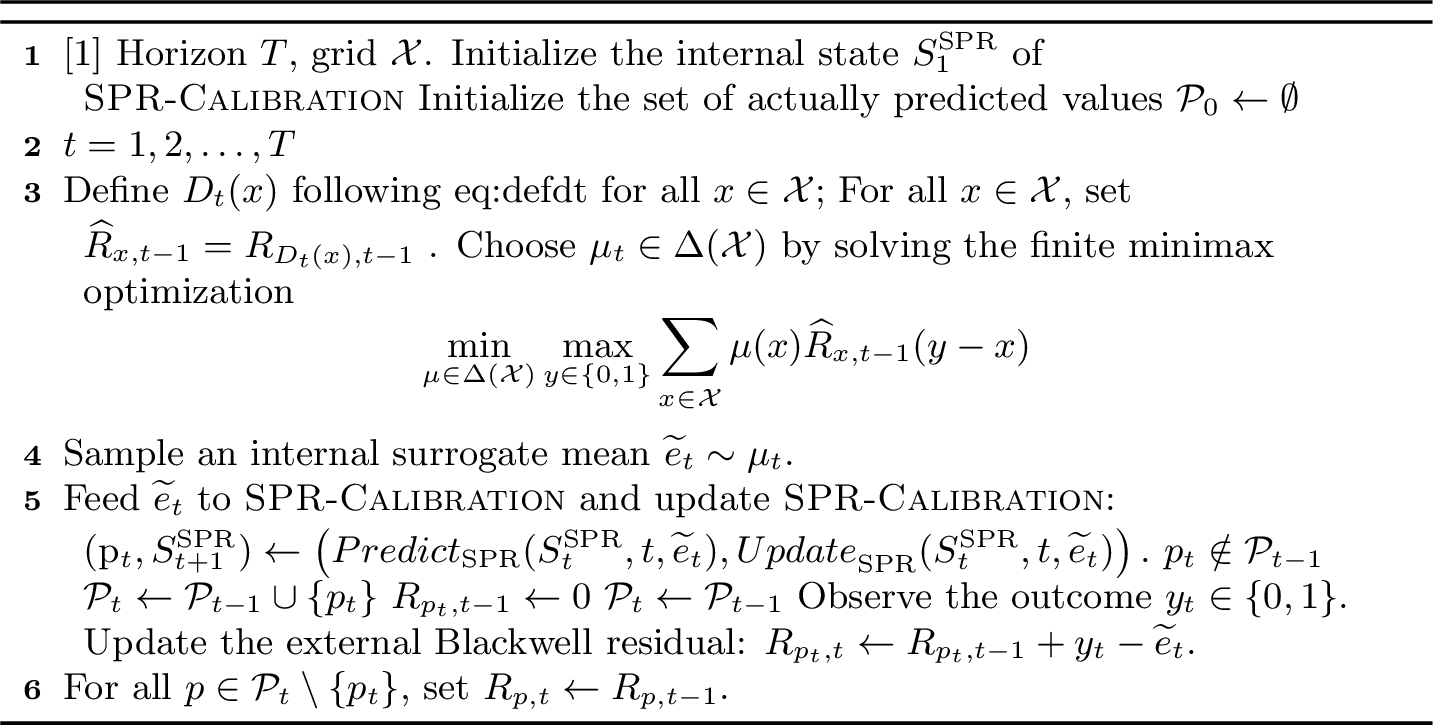
We present our main algorithm in Algorithm 5. The algorithm maintains an instance of SPR-Calibration. The main difficulty in applying SPR-Calibration is that the conditional means \(\{e_t\}_{t=1}^T\) are not available to the forecaster. To address this, we use a Blackwell-style correction layer to construct, at each round \(t\in[T]\), a surrogate estimate \(\widetilde{e}_t\) of \(e_t\). This surrogate is then passed as the input to the SPR-Calibration instance.
Let \(\mathcal{X} =\{0, \eta, 2\eta,\ldots, N\eta \}\) be a grid with threshold \(\eta = T^{-1/2}\) and \(N =\left\lfloor 1/\eta\right\rfloor\).
At each round \(t\), let \(S_t^{\mathrm{SPR}}\) denote the internal state of the SPR-Calibration instance used by Algorithm 5 before round \(t\) and \(\mathcal{P}_t = \{ p_s: s\leq t\}\). For each \(x\in \mathcal{X}\) and \(p\in \mathcal{P}_{t-1}\), we define
\[\begin{align} D_t(x) & := \operatorname{Predict}_{\mathrm{SPR}}( S^{\mathrm{SPR}}_t,t ,x)\tag{3} \\ R_{p, t-1} & : = \sum_{s<t: p_s =p} (y_s - \tilde{e}_s)\tag{4} \end{align}\]
Moreover, for each \(x\in\mathcal{X}\), define \(\widehat R_{x,t-1}:=R_{D_t(x),t-1}.\) In particular, if \(D_t(x)\notin\mathcal{P}_{t-1}\), we use the default initialization \(\widehat R_{x,t-1} = R_{D_t(x),t-1} = 0.\)
Given the quantities \(\widehat R_{x,t-1}\) defined above, we solve the following Blackwell-style minimax program to obtain an optimal distribution \(\mu_t\in\Delta(\mathcal{X})\), where \(\Delta(\mathcal{X})\) denotes the set of probability distributions over \(\mathcal{X}\). \[\begin{align} \beta_t = \min_{\mu\in\Delta(\mathcal{X})} \max_{y\in\{0,1\}} \sum_{x\in\mathcal{X}} \mu(x)\widehat{R}_{x, t-1}(y-x).\label{eq:opt} \end{align}\tag{5}\]
Then the algorithm samples the surrogate mean \(\widetilde{e}_t\sim \mu_t\), and commits the deterministic SPR-Calibration steps: \[\begin{align} p_t = D_t(\widetilde{e}_t) & = \operatorname{Predict}_{\mathrm{SPR}} (S_t^{\mathrm{SPR}},t,\widetilde{e}_t), \nonumber \\S_{t+1}^{\mathrm{SPR}} & = \operatorname{Update}_{\mathrm{SPR}} (S_t^{\mathrm{SPR}},t,\widetilde{e}_t).\nonumber \end{align}\]
After outputting the forecast \(p_t\) and observing the true outcome \(y_t\), we update \(\mathcal{P}_t\) and the residuals \(R_{p,t}\) for all \(p\in\mathcal{P}_t\).
5 Analysis↩︎
In this section, we present the proof of Theorem 1. The proof consists of two parts: bounding the calibration error and the computational cost.
5.1 Proof of Calibration Error↩︎
Set the hyperparameters of SPR-Calibration as \(\tau=\left\lceil \log_2 T\right\rceil\), and choose the scale parameter \(h\leq \tau\) later. Recall \(\mathcal{P}_t=\{p_s:s\le t\}\). For \(t\in [T]\) and \(p\in \mathcal{P}_t\), recall the outer residual \(R_{p,t} = \sum_{s\le t:p_s=p}(y_s-\widetilde{e}_s)\) if \(p\in \mathcal{P}_t\). Define \(R_{p,t} = 0\) if \(p\notin \mathcal{P}_t\).
For every \(p\in\mathcal{P}_T\), \[\sum_{t\in [T]: p_t = p}(y_t-p) = \sum_{t\in [T]: p_t = p}(\widetilde{e}_t-p) + \sum_{t\in [T]: p_t = p}(y_t-\widetilde{e}_t).\] Therefore, \[\begin{align} \mathbb{E}[\operatorname{CalErr}_T] \le \underbrace{\mathbb{E}\left[ \sum_{p\in\mathcal{P}_T} \left| \sum_{t\in [T]: p_t = p}(\widetilde{e}_t-p) \right|\right] }_{\text{\mathrm{\small SPR-Calibration} bias term}} + \underbrace{ \mathbb{E}\left[\sum_{p\in\mathcal{P}_T}|R_{p,T}|\right] }_{\text{Blackwell residual term}}. \end{align}\]
5.1.0.1 Bound of the SPR-Calibration bias term.
The bound of the SPR-Calibration bias directly follows the result in [1]. By Lemma 4, we have that \[\begin{align} \mathbb{E}\left[ \sum_{p\in\mathcal{P}_T} \left| \sum_{t\in [T]: p_t = p}(\widetilde{e}_t-p) \right|\right] \leq O\!\left( \sum_{i=1}^{\tau-h} \sum_{j=i+1}^{i+h} 2^{j-i} 2^{\gamma(i+\tau-j)} + \sum_{i\leq \tau - h} \sum_{j\leq i+h}\min\{ 2^i ,2^{\tau-h-i}\} \right).\label{eq:boundB} \end{align}\tag{6}\]
5.1.0.2 Bound of the Blackwell residual term.
By the property of SPR-Calibration (see Lemma 2), we have that \(|\mathcal{P}_T|\le O\!\left(2^{(\tau-h)/2}\right).\) Then by Cauchy’s inequality, we have that \[\begin{align} \mathbb{E}\left[\sum_{p\in \mathcal{P}_T} \left| R_{p,T} \right|\right]\leq O\left( \sqrt{ 2^{(\tau-h)/2} \mathbb{E}\left[\sum_{p\in \mathcal{P}_T}R_{p,T}^2\right]} \right)\leq O\left( \sqrt{ \mathbb{E}[\Phi_T]}\cdot 2^{(\tau-h)/4}\right),\label{eq:boundP1} \end{align}\tag{7}\] where we define \(\Phi_t =\sum_{p\in \mathcal{P}_t}R_{p,t}^2\) for \(t\in [T]\) and \(\Phi_0 = 0\). Then we have the following lemma to bound \(\mathbb{E}[\Phi_T]\).
Lemma 5. \(\mathbb{E}[\Phi_T] = O\!\left((\sqrt T+\eta T)^2\right)\). If \(\eta = O( T^{-1/2})\), then \(\mathbb{E}[\Phi_T] = O(T)\).
By Lemma 5 and 7 , we have that \(\mathbb{E}\left[\sum_{p\in \mathcal{P}_T} \left| R_{p,T} \right|\right]\leq O(\sqrt{T}\cdot 2^{(\tau-h)/4})\).
5.1.0.3 Putting all together.
Recall that \(\eta = T^{-1/2}\). Let \(\varepsilon_{\mathrm{AB}}\) be defined in Lemma 3 and let \(\gamma = \frac{1-\varepsilon_{\mathrm{AB}} }{2- \varepsilon_{\mathrm{AB}}}\). We then have that \[\begin{align} & \mathbb{E}[\operatorname{CalErr}_T] \nonumber \\ & \leq O\!\left( \sum_{i=1}^{\tau-h} \sum_{j=i+1}^{i+h} 2^{j-i} 2^{\gamma(i+\tau-j)} + \sum_{i=1}^{\tau-h} \sum_{j\leq i+h}\min\{ 2^i ,2^{\tau-h-i}\} \right) + O\left( \sqrt{T}\cdot 2^{(\tau-h)/4}\right) \nonumber \\ & \leq O\left(\sum_{i=1}^{\tau-h} 2^{h(1-\gamma) + \gamma\tau } + \log_2(T)\cdot \sum_{i\leq \tau -h} \min\{2^i, 2^{\tau-h-i}\} +\sqrt{T}\cdot 2^{(\tau-h)/4} \right) \nonumber \\ & \leq O\left( \log_2(T) \cdot 2^{h+\gamma(\tau -h)} + \log_2(T) \cdot 2^{(\tau-h)/2} + \sqrt{T} \cdot 2^{(\tau-h)/4}\right) \tag{8} \\ & \leq O\!\left(\log_2(T)\cdot 2^{h+\gamma(\tau-h)}+\log_2(T)\cdot 2^{3\tau/4-h/4} \right).\tag{9} \end{align}\] Here, 8 follows from the inequality \(j-i\le h\) and the fact that \(\sum_{i=1}^{\tau-h} \min\{ 2^i, 2^{\tau-h-i}\} = O(2^{(\tau-h)/2})\), while 9 follows from \((\tau-h)/2\le 3\tau/4-h/4\).
By choosing \(h = \frac{3-4\gamma}{5-4\gamma}\tau = \frac{2+\varepsilon_{\mathrm{AB}}}{6-\varepsilon_{\mathrm{AB}}} \tau\), we have that \(\mathbb{E}[\operatorname{CalErr}_T]\leq O\left(\log_2(T)\cdot T^{\frac{2}{3} - \frac{\varepsilon_{\mathrm{AB}}}{18}}\right)\).
5.2 Computational cost↩︎
We give a fully explicit implementation of Algorithm 5. The purpose of the argument is only to establish a polynomial running time, so we use direct scans and deep copies rather than more sophisticated persistent data structures. Let \(K = \left\lceil 1/\eta \right\rceil\). Recall also that \(\tau=\left\lceil\log_2T\right\rceil\), \(\overline{T}=2^\tau<2T\) and \(h\le \tau-1\).
Lemma 6. Algorithm 5, using the deterministic transition from Section 3.1 and the explicit \(A/B\) labeler, can be implemented in time \(O\!\left(T^{\frac{7}{2}}\log T\right)\).
Proof. We prove by bounding the cost of one deterministic SPR transition and the additional work performed by the outer wrapper.
5.2.0.1 Size of the SPR state.
For every \(i\in\mathcal{I}_h=\{1,\ldots,\tau-h\}\), \(j\in\mathcal{J}_i=\{i+1,\ldots,i+h\}\) and \(\ell\in\{0,1\}\), the algorithm maintains a board \(G_{i,j,\ell}\) with \(2^i\) cells. Its bias array and sign array use \(O(2^i)\) words.
The live state of the explicit \(A/B\) labeler also uses \(O(2^i)\) words. Indeed, its recursively stored objects form a binary tree with \(O(2^i)\) nodes, and every node stores only a constant number of counters, pointers, phase variables, and integer parameters. When a labeler object is restarted, the old object is discarded, so obsolete versions are not retained.
Thus, one board requires \(O(2^i)\) words, and the local SPR state has size \[\begin{align} \sum_{i=1}^{\tau-h} \sum_{j=i+1}^{i+h} \sum_{\ell\in\{0,1\}} O(2^i) &= O\!\left( h\sum_{i=1}^{\tau-h}2^i \right)= O\!\left( h2^{\tau-h} \right). \end{align}\] Taking the historical recording of the local SPR states into consideration, the complete SPR state has size \(O(Th 2^{\tau-h})\). The same bound applies to the one-time initialization cost and to the cost of making a deep copy of the state.
5.2.0.2 Cost of one SPR transition.
Consider \(\operatorname{Step}_{\mathrm{SPR}}(S,t,z)\) for a fixed input \(z\in[0,1]\). In the bias-removal phase, for each pair \((i,j)\), the parity of
\(z\) selects one of the two boards \(G_{i,j,0}\) and \(G_{i,j,1}\). A direct scan of that board finds an admissible cell in \(O(2^i)\) time if one exists. Hence a complete bias-removal scan costs \(O\!\left( h\sum_{i=1}^{\tau-h}2^i \right) = O\!\left( h2^{\tau-h} \right).\) The bias-placement phase performs only \(O(h\tau)\) constant-time current-cell checks, except that it may make one call to simulateGame. Suppose that simulateGame is called on a board with \(2^i\) cells.
Scanning the sign array, constructing the reduced transcripts, and carrying out all else legal deletions costs \(O(2^i)\),
It remains to bound the cost of the \(A/B\) label query. A call to the recursive \(A/B\) procedure follows a root-to-leaf path of depth at most \(i\). At each depth, the corresponding \(A\)-object can restart its current \(B\)-object at most once before returning a sign. Eagerly initializing a \(B\)-object on an interval of length at most \(2^i\) costs \(O(2^i)\). Therefore, the deliberately coarse bound \(O(i2^i) \le O\!\left( \tau2^{\tau-h} \right)\) holds for one label query.
Combining the bias-removal phase, the bias-placement phase, and the possible game simulation gives that the time cost of \(\operatorname{Step}_{\mathrm{SPR}}(S,t,z)\) is bounded by \(O(\tau 2^{\tau-h})\).
5.2.0.3 Computing all preview predictions.
For each \(x\in\mathcal{X}\), the algorithm:
makes a deep copy of \(S_t^{\mathrm{SPR}}\);
evaluates \(\operatorname{Step}_{\mathrm{SPR}} (S_t^{\mathrm{SPR}},t,x)\) on the scratch copy;
records only the resulting prediction \(D_t(x)\); and
discards the scratch copy.
Consequently, computing all \(K\) values \(D_t(x)\) costs \(O\!\left( TK\tau2^{\tau-h} \right)\) time. Because the scratch state is reused, this requires only one scratch copy, rather than \(K\) simultaneous copies.
5.2.0.4 Solving the finite minimax problem.
The minimax optimization problem 5 has \(K\) variables, corresponding to the distribution over the \(K\) grid points, and only two constraints, corresponding to the two possible outcomes \(y=0\) and \(y=1\). Therefore, it can be solved within \(O(K^2)\) time.
5.2.0.5 Putting all together.
After sampling \(\widetilde{e}_t\), the algorithm commits exactly one SPR transition: \[(p_t,S_{t+1}^{\mathrm{SPR}}) = \operatorname{Step}_{\mathrm{SPR}} (S_t^{\mathrm{SPR}},t,\widetilde{e}_t).\] This costs \(O\!\left( \tau2^{\tau-h} \right)\). Therefore, the total cost of round \(t\) is \(O\!\left( TK\tau2^{\tau-h}+K^2 \right).\) Summing over the \(T\) rounds and including the one-time initialization cost gives \(O\!\left( T^2K\tau2^{\tau-h}+TK^2 \right).\) Using \(K=O(\sqrt T)\), \(\tau=O(\log T)\), and \(2^{\tau-h}\le 2^\tau<2T\), we obtain \[\begin{align} O\left( T^2K\tau2^{\tau-h}+TK^2\right) = O\!\left( T^{\frac{7}{2}}\log T \right).\nonumber \end{align}\] ◻
5.3 Proof of Lemma 5↩︎
Lemma 5 (restatement). \(\mathbb{E}[\Phi_T] = O\!\left((\sqrt T+\eta T)^2\right)\). If \(\eta = O( T^{-1/2})\), then \(\mathbb{E}[\Phi_T] = O(T)\).
Proof. Recall that \(\mathcal{X}\) is the grid with interval length \(\eta\). At round \(t\), the wrapper chooses a distribution \(\mu_t\in\Delta(\mathcal{X})\) by solving the finite minimax problem 5 as \[\begin{align} \beta_t = \min_{\mu\in\Delta(\mathcal{X})} \max_{y\in\{0,1\}} \sum_{x\in\mathcal{X}} \mu(x)\widehat{R}_{x, t-1}(y-x).\nonumber \end{align}\]
By Von Neumann’s minimax theorem \[\begin{align} \beta_t & = \max_{q\in\Delta(\{0,1\})} \min_{x\in\mathcal{X}} \mathbb{E}_{y\sim q}\left[\widehat{R}_{x, t-1}(y-x)\right] \nonumber \\ & = \max_{q\in\Delta(\{0,1\})} \min_{x\in\mathcal{X}} \widehat{R}_{x, t-1}(\mathbb{E}_{y\sim q}[y]-x) \nonumber \\ &= \max_{y\in [0,1]} \min_{x\in\mathcal{X}} \widehat{R}_{x, t-1}(y-x). \label{eq:optdual} \end{align}\tag{10}\] Fix any \(y\in[0,1]\), and let \(x^*(y)\in\arg\min_{x\in\mathcal{X}}|y-x|\). Then \(|y-x^*(y)|\le\eta.\) Therefore, \[\min_{x\in \mathcal{X}}\widehat{R}_{x, t-1}(y-x) \le \left|\widehat{R}_{x^*(y), t-1}\right| \eta.\] Since \(\left|\widehat{R}_{x^*(y), t-1}\right| \le \sqrt{\Phi_{t-1}}\), we have \(\min_{x\in\mathcal{X}} \widehat{R}_{x^*(y), t-1}(y-x) \le \eta\sqrt{\Phi_{t-1}}.\) Taking the maximum over \(y\in[0,1]\) gives \(\beta_t\le \eta\sqrt{\Phi_{t-1}}.\) Since \(\mu_t\) is optimal for the finite minimax problem, for both \(y\in\{0,1\}\), \(\mathbb{E}_{x\sim\mu_t} \left[ \widehat{R}_{x, t-1}(y-x) \right] \le \beta_t \le \eta\sqrt{\Phi_{t-1}}\). Recalling that \(\widehat{R}_{x,t-1} = R_{D_t(x), t-1}\) for all \(x\in \mathcal{X}\), we always have \[\begin{align} \mathbb{E}_{x\sim\mu_t} \left[ R_{D_t(x), t-1}(y_t-x) \right] \le \beta_t \le \eta\sqrt{\Phi_{t-1}}.\label{eq:us1} \end{align}\tag{11}\]
Let \(\mathcal{F}_{t}\) denote the \(\sigma\)-field after the \(t\)-th round. So the adversary chooses \(y_t\) (or its distribution) conditioned on \(\mathcal{F}_t\). We then have that \[\begin{align} \mathbb{E}[\Phi_t-\Phi_{t-1}\mid\mathcal{F}_{t-1}] = \mathbb{E}_{x\sim \mu_t}[2R_{D_t(x), t-1}(y_t-x)+(y_t-x)^2 \mid \mathcal{F}_{t-1}]\leq 2\eta \sqrt{\Phi_{t-1}} + 1,\nonumber \end{align}\] which implies \[\begin{align} \mathbb{E}[\Phi_t] - \mathbb{E}[\Phi_{t-1}]\leq 2\eta \mathbb{E}[\sqrt{\Phi_{t-1}}] + 1.\nonumber \end{align}\] Let \(Z_t=\mathbb{E}[\Phi_t]\) for \(t\geq 0\). By Jensen’s inequality, \(\mathbb{E}[\sqrt{\Phi_{t-1}}]\le \sqrt{Z_{t-1}}.\) Therefore, \[Z_t \le Z_{t-1}+1+2\eta\sqrt{Z_{t-1}}.\] Summing over \(t\) yields \(Z_T \le T+2\eta\sum_{t=0}^{T-1}\sqrt{Z_t}\). Let \(M_T=\max_{0\le t\le T}\sqrt{Z_t}.\) Then \(M_T^2 \le T+2\eta T M_T.\) Solving this quadratic inequality gives \[M_T \le \eta T+\sqrt{\eta^2T^2+T} \le 2\eta T+\sqrt T.\] Hence \[Z_T \le M_T^2 \le O\!\left((\sqrt T+\eta T)^2\right).\] If \(\eta\le T^{-1/2}\), then \(\sqrt T+\eta T=O(\sqrt T)\), and therefore \(\mathbb{E}[\Phi_T]=O(T)\). ◻
6 Discussion↩︎
In this paper, we develop an efficient algorithm that achieves \(O(T^{2/3-\varepsilon})\) calibration error. Our algorithm is based on a simple combination of the SPR-Calibration algorithm in [1] and a Blackwell-approachability correction argument. The resulting improvement exponent \(\varepsilon\) is inherited from the SPR guarantee in [1]; in particular, any improvement in the value of the underlying SPR game would translate directly into a stronger efficient calibration bound.
References↩︎
We use this half-open interval convention to make the interval assignment explicit.↩︎