Accelerated Mixing Time of Randomized Hamiltonian Monte Carlo
July 14, 2026
Abstract
We show the Randomized Hamiltonian Monte Carlo (RHMC) algorithm has accelerated mixing time guarantees for sampling from log-concave probability distributions. RHMC proceeds by repeatedly simulating the continuous-time Hamiltonian dynamics for some random integration times, and resetting the velocity to be an independent Gaussian random variable between each simulation. We show that when the target distribution is log-concave and satisfies an \(\alpha\)-Talagrand inequality (for example, if the target distribution is \(\alpha\)-strongly log-concave), if we use a random integration time from either the triangular or the exponential distribution with mean \(\Theta(\alpha^{-1/2})\), then RHMC converges exponentially fast in KL divergence, and the total integration time to reach error \(\varepsilon\) in KL divergence scales as \(O(\alpha^{-1/2} \log(\varepsilon^{-1}))\). We also show that when the target distribution is log-concave, if we use a sequence of random integration times from the triangular distribution with exponentially increasing means, then the total integration time to reach error \(\varepsilon\) in KL divergence scales as \(O(\varepsilon^{-1/2})\). Our analysis relies on a bound on the average KL divergence along Hamiltonian dynamics, which is inspired by an analogous result on accelerated optimization methods based on Hamiltonian dynamics.
1 Introduction↩︎
Drawing samples from a probability distribution is an essential algorithmic task in many areas of science and engineering. A popular class of techniques for performing sampling is by running an ergodic Markov chain whose stationary distribution is the target probability distribution; such techniques are referred to as Markov Chain Monte Carlo (MCMC) [1]. The efficiency of an MCMC algorithm is dictated by its mixing time — this quantifies how quickly the Markov chain converges to the stationary distribution. In practice, many sampling algorithms are based on time-discretizations of continuous-time dynamics, including the overdamped or underdamped Langevin dynamics, which are stochastic processes, and the Hamiltonian dynamics, which is deterministic. In this paper, we focus on the Randomized Hamiltonian Monte Carlo (RHMC) algorithm, which is based on simulating the Hamiltonian dynamics for times that are randomized, and show that it achieves accelerated mixing time guarantees.
To contextualize our results for RHMC, we briefly review relevant guarantees for the overdamped and underdamped Langevin dynamics, which have been studied in more detail. We denote the target distribution that we aim to draw samples from by \(\nu^{X}\). The overdamped Langevin dynamics (LD) [2] is a basic stochastic process for sampling \(\nu^{X}\) by taking into account the gradient of the log density of \(\nu^{X}\). Langevin dynamics has a natural optimization interpretation as the gradient flow dynamics (in the space of probability measures equipped with the Wasserstein metric) to minimize the relative entropy or Kullback-Leibler (\(\mathsf{KL}\)) divergence with respect to the target distribution [3]. Partly motivated by this optimization perspective, there have been many works that result in a rich understanding of the mixing time of LD and its algorithmic implementations under various structural assumptions on the target distribution. The mixing times discussed here depend on (a) the measure of discrepancy, and (b) the error level \(\varepsilon\) to the target. We highlight two key results that are particularly relevant to our work:
when \(\nu^{X}\) satisfies an \(\alpha\)-log-Sobolev inequality (see 2.1.3 for a definition), the \(\mathsf{KL}\)-mixing time for error \(\varepsilon\) of LD scales as \(\alpha^{-1} \log (\varepsilon^{-1})\) [4], and
when \(\nu^{X}\) is log-concave (see 2.1.2 for a definition), the \(\mathsf{KL}\)-mixing time for error \(\varepsilon\) scales as \(\varepsilon^{-1}\) [5].
Notably, these rates match the time complexities of the Euclidean gradient flow for minimizing a function \(f\) that satisfies \(\alpha\)-gradient domination (implied by \(\alpha\)-strong convexity) and convexity, respectively, to within \(\varepsilon\) of the optimal value. There are also guarantees for time discretizations of LD, which we do not discuss further since in this paper we focus on the continuous-time complexity.
Motivated by the algorithmic applications, as well as taking inspiration from the theory of acceleration in convex optimization, there have been several efforts made towards identifying other dynamics that mix faster. To be more specific, we seek analogues of the following results from convex optimization for the accelerated gradient flow [6], [7] for the time complexities to within \(\varepsilon\) of than the optimal value:
for a function that is \(\alpha\)-strongly convex, the time complexity scales as \(\alpha^{-1/2} \log(\varepsilon^{-1})\), and
for a function that is convex, the time complexity scales as \(\varepsilon^{-1/2}\).
A candidate dynamics is the underdamped Langevin dynamics (ULD) which is a stochastic process defined on the phase space of both position and velocity. In ULD, the evolution of the position is deterministically governed by the velocity, and the evolution of the velocity is encoded as a stochastic process involving the gradient of the log density of \(\nu^{X}\). The ULD is a natural dynamics to consider primarily owing to the structural similarities to the accelerated gradient flow referenced earlier, and many works have studied whether ULD has faster convergence guarantees compared to LD (see for instance, [8], [9]). Indeed ULD has been shown to have an accelerated convergence guarantee; in particular, [10] show ULD has a \(\chi^{2}\)-mixing time for error \(\varepsilon\) that scales as \(\alpha^{-1/2}\log(\varepsilon^{-1})\) when \(\nu^{X}\) is log-concave and satisfies an \(\alpha\)-Poincaré inequality (implied when \(\nu^X\) satisfies \(\alpha\)-log Sobolev inequality). [11] recently shows that ULD also has \(\mathsf{KL}\)-mixing time for error \(\varepsilon\) that scales as \(\alpha^{-1/2}\log(\varepsilon^{-1})\) when \(\nu^{X}\) is both log-concave and satisfies an \(\alpha\)-log-Sobolev inequality. This strictly improves on the \(\mathsf{KL}\)-mixing time scaling of LD (while additionally assuming log-concavity), and also matches the accelerated convergence rate we expect from optimization. When \(\nu^{X}\) is only log-concave, [12] show that ULD has a \(\mathsf{KL}\)-mixing time for error \(\varepsilon\) that scales as \(\varepsilon^{-1}\), which is the same scaling achieved by LD; the accelerated rate of \(\varepsilon^{-1/2}\) seems unknown for ULD.
The Hamiltonian dynamics is a deterministic process on the phase space of position and velocity that conserves the Hamiltonian or energy function. The Hamiltonian Monte Carlo (HMC) algorithm [13] is a piecewise-deterministic Markov chain that proceeds iteratively by (a) simulating the Hamiltonian dynamics for some integration time, and (b) resetting the velocity to be an independent Gaussian random variable. HMC and its variants are some of the most widely used sampling algorithms in practice, and underlie probabilistic programming systems such as Stan [14] and PyMC [15]. Despite its practical importance, the theoretical guarantees of HMC and its variants are less developed than LD or ULD. Many existing results focus on the short integration time, where the time to simulate the Hamiltonian flow between velocity resetting scales inversely with the smoothness of the target distribution. With short integration time, HMC has unaccelerated convergence guarantees similar to LD and with additional dependence on the smoothness. [16] show that when \(\nu^{X}\) is strongly log-concave (see 2.1.2 for a definition) and \(L\)-log smooth, the \(\mathsf{W}_{2}\)-mixing time of HMC(i.e., iterations) for error \(\varepsilon\) scales as \(L\alpha^{-1}\log(\varepsilon^{-1})\) where each iteration simulates the Hamiltonian dynamics for integration time \(L^{-1/2}\) (the “short” integration time) [16] and thus implies a total integration time that scales as \(L^{1/2}\alpha^{-1} \log(\varepsilon^{-1})\). This result is also shown to be tight via a matching lower bound. Later work by [17] improve this result by generalizing to target distributions that satisfy a \(\alpha\)-log-Sobolev inequality and are \(L\)-log-smooth, and providing a \(\mathsf{KL}\)-mixing time of the same order.
Hence, additional ideas are required to obtain faster convergence rates for HMC; in fact, not only are deterministic integration times unable to obtain accelerated mixing time guarantees [16], deterministic and long integration times that scale inversely with the curvature lower bound as \(\alpha^{-1/2}\) can fail to make any progress at all, as this integration time coincides with the natural oscillation frequencies of the dynamics, e.g., even for Gaussian target distributions. This motivates the Randomized Hamiltonian Monte Carlo (RHMC) [18], which randomizes the integration times between velocity refreshments. RHMC with suitably randomized integration times are conjectured to achieve accelerated convergence guarantees, see e.g., [19]. Toward this conjecture, [20] show that when the target distribution is log-concave and satisfies \(\alpha\)-Poincaré inequality, RHMC reaches error \(\varepsilon\) in chi-square divergence in an expected total integration time that scales as \(\alpha^{-1/2} \log(\varepsilon^{-1})\). A recent work by [21], extending the technique of [11], [22], show that when the target distribution is log-concave and satisfies an \(\alpha\)-log-Sobolev inequality, RHMC reaches error \(\varepsilon\) in KL divergence in an expected total integration time \(\alpha^{-1/2}\log(\varepsilon^{-1})\), which matches the desired accelerated rate from optimization.
In this work, we establish accelerated mixing-time guarantees for RHMC in KL divergence in two settings: (a) when the target distribution is semi-log-concave and satisfies Talagrand inequality, we obtain a result which matches [21]; and (b) when the target distribution is log-concave, we obtain a new result. The accelerated mixing time guarantees for RHMC in all of these works also overcome the dependence on the smoothness parameter which is present in works studying deterministic integration times. We provide additional discussion on related work in 6.
In addition to the RHMC algorithm presented in [18] and studied in [20], [21], which considers the integration time to be drawn from an exponential distribution, we also consider RHMC with integration time drawn from a triangular distribution; this has the benefit of being compactly supported, and therefore guarantees on the total integration time hold deterministically instead of in expectation. We describe these RHMC algorithms in 1.1 and describe our results in more detail in 1.2.
1.1 Randomized Hamiltonian Monte Carlo↩︎
We introduce the Randomized Hamiltonian Monte Carlo (RHMC) algorithm studied in this paper; see 1 below. Our goal is to sample from a target distribution \(\nu^X\) with full support on \(\mathbb{R}^d\). We assume the target distribution has density function \(\nu^X \propto e^{-f}\) for some potential function \(f \colon \mathbb{R}^d \to \mathbb{R}\). The RHMC algorithm is based on the Hamiltonian dynamics. Consider the phase space \(\mathbb{R}^{2d} = \mathbb{R}^d \times \mathbb{R}^d\), which consists of the joint position and velocity variables. We define the Hamiltonian function \(H \colon \mathbb{R}^{2d} \to \mathbb{R}\) by, for all \((x,y) \in \mathbb{R}^{2d}\), \[\begin{align} \label{Eq:HamDef} H(x,y) \mathrel{\vcenter{:}}= f(x) + \frac{1}{2} \|y\|^2 \,. \end{align}\tag{1}\] Given the Hamiltonian function 1 , the Hamiltonian dynamics or Hamiltonian flow is the evolution of the joint variables \((X_t, Y_t) \in \mathbb{R}^{2d}\) following the system of ordinary differential equations: \[\label{eq:HamFlow} } \begin{align} \dot{X}_{t} &= \nabla_y H(X_t,Y_t) = Y_t \\ \dot{Y}_{t} &= -\nabla_x H(X_t,Y_t) = -\nabla f(X_t) \end{align}\tag{2}\] starting from any initial configuration \((X_0, Y_0) \in \mathbb{R}^{2d}\) at time \(t = 0\).
The RHMC algorithm proceeds by evolving along the dynamics 2 combined with periodic velocity refreshment from the standard Gaussian distribution \(\mathcal{N}(0, \mathrm{I}_d)\). We describe the RHMC algorithm formally in 1.
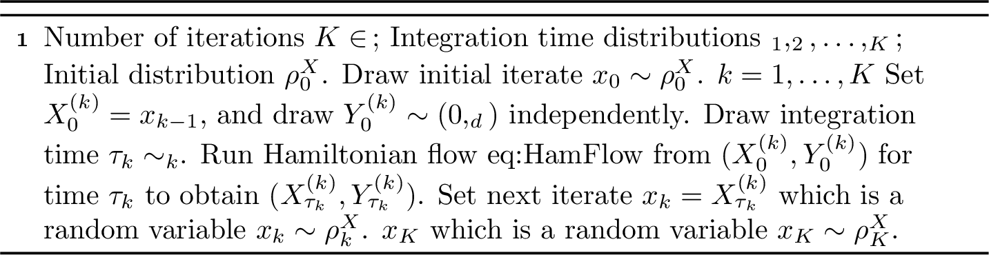
Randomized Hamiltonian Monte Carlo (RHMC), presented in 1, corresponds to a suite of algorithms, with different choices of integration time distributions \(\mathcal{D}_1, \dots, \mathcal{D}_{K}\) corresponding to different algorithms. When \(\mathcal{D}_k = \delta_T\) for some \(T>0\), or equivalently, \(\tau_k = T\) is deterministic for all \(k \in \{1, \dots, K\}\), the algorithm is referred to as Hamiltonian Monte Carlo (HMC); see 6 for a discussion of works studying HMC. We study the RHMC algorithm where the integration time distributions \(\mathcal{D}_1, \dots, \mathcal{D}_{K}\) are not degenerate, as studied in [18], [23]–[25].
We study 1 with the following choices of integration time distributions:
In the setting [Set-Tri], we study 1 with \[\mathcal{D}_k \mathrel{\vcenter{:}}=\mathsf{Tri}_T \text{~~with~~} T > 0 \text{~~for all~~} k \in \{1, \dots, K\} \,.\] Here \(\mathsf{Tri}_T\) is the triangular distribution with parameter \(T>0\), which is supported on \([0,T]\) with density function at \(t \in [0,T]\) given by: \[\label{eq:TriangularDensityFunction} \mathsf{Tri}_T(t) \mathrel{\vcenter{:}}=\frac{2}{T^2}(T-t)\,.\tag{3}\]
The choice of triangular integration time distributions in [Set-Tri] is motivated by studying the analogue of 1 for optimization; see 7 for a discussion. We also note that the choice of triangular integration time is similar to the adaptive stopping time of Hamiltonian dynamics-based No-U-Turn Sampler (NUTS) which is widely used in practice [26].
In the setting [Set-Exp], we study 1 with \[\mathcal{D}_k \mathrel{\vcenter{:}}=\mathsf{Exp}_{1/T} \text{~~with~~} T > 0 \text{~~for all~~} k \in \{1, \dots, K\} \,.\] Here \(\mathsf{Exp}_{1/T}\) is the exponential distribution supported on \([0,\infty)\) with parameter \(\frac{1}{T}>0\), with density function given by, for all \(t \in [0,\infty)\), \[\label{eq:ExponentialDensityFunction} \mathsf{Exp}_{1/T}(t) \mathrel{\vcenter{:}}=\frac{1}{T} \exp\Big(-\frac{t}{T}\Big) \,.\tag{4}\] The mean of \(\mathsf{Exp}_{1/T}\) is \(T\), i.e., \(\mathbb{E}_{\tau \sim \mathsf{Exp}_{1/T}}[\tau] = T\). We will use the fact that \(\mathsf{Exp}_{1/T}\) can be represented as a mixture of triangular distributions; see 4. The RHMC algorithm with exponentially distributed integration times was proposed in [18].
In the setting [Set-\(\widetilde{\mathsf{Tri}}\)], we study 1 with \[\mathcal{D}_k \mathrel{\vcenter{:}}=\widetilde{\mathsf{Tri}}_{T_k} \text{~~for some~~} T_{k} > 0 \text{~~for all~~} k \in \{1, \dots, K\}\,.\] Here for any \(T>0\), \(\widetilde{\mathsf{Tri}}_T\) refers to the endpoint-biased triangular distribution given by \[\widetilde{\mathsf{Tri}}_T \mathrel{\vcenter{:}}=\frac{1}{2} \delta_{T} + \frac{1}{2} \mathsf{Tri}_T\,.\] Like [Set-Tri], the choice of the integration time distribution in this setting is motivated by studying the analogue of 1 for convex optimization; see 7 for more details.
1.2 Our contributions↩︎
In this work, we prove convergence guarantees for the idealized RHMC algorithm in 1 under several assumptions on the target distribution. Here idealized means we assume we can simulate the Hamiltonian flow 2 exactly. We measure the complexity of RHMC by the total amount of integration time required to simulate the Hamiltonian flow in order to reach a prescribed error in KL divergence.
Our first result concerns target distributions \(\nu^X\) that satisfy \(\alpha\)-Talagrand inequality (see 2.1.3) and are \(M\)-semi-log-concave (see 2.1.2) for some \(0\leq M<\alpha\). In this setting, we prove a convergence guarantee in KL divergence for RHMC with integration times drawn from either the triangular or exponential distribution with mean \(\Theta((\alpha-M)^{-1/2})\). As we show in 1, to obtain \(\mathsf{KL}(\rho_K^X\mathbin{\|}\nu^X)\leq \varepsilon\), it suffices to simulate Hamiltonian flow for a total integration time \[O\left( \frac{1}{\sqrt{\alpha-M}} \log\frac{\mathsf{KL}(\rho_0^X\mathbin{\|}\nu^X)}{\varepsilon} \right) \,.\] When using [Set-Tri], this upper bound is deterministic. When using [Set-Exp], this is an upper bound on the expected total integration time. In particular, when \(M=0\) (i.e., when \(\nu^X\) is log-concave), this gives a total integration time \(O(\alpha^{-1/2} \log(\varepsilon^{-1})),\) which improves over the \(O(\alpha^{-1} \log(\varepsilon^{-1}))\) time of the overdamped Langevin dynamics in the same setting, and matches the result of [21].
Our second result concerns the log-concave case, without assuming Talagrand inequality. In this setting, we use an endpoint-biased triangular distribution \(\widetilde{\mathsf{Tri}}_{T_k}=\frac{1}{2}\delta_{T_k}+\frac{1}{2}\mathsf{Tri}_{T_k}\), with integration-time parameter \(T_k\) increasing with iteration \(k\). We show in 2 a convergence guarantee in KL divergence, which implies (see 2) that to obtain error \(\varepsilon\) in KL divergence, it suffices to simulate Hamiltonian flow for total integration time \[O\left( \sqrt{ \frac{ \mathsf{KL}(\rho_0^X\mathbin{\|}\nu^X) +\frac{1}{3}\mathsf{W}_2^2(\rho_0^X,\nu^X)}{\varepsilon}} \right) \,.\] This improves the \(O(\varepsilon^{-1})\) time of the overdamped Langevin dynamics in this setting, and matches what we expect from the theory of accelerated convex optimization.
Our analysis is inspired by translating the proofs from the Hamiltonian dynamics-based optimization method of [27] to the sampling setting, in particular to the space of probability distributions with the Wasserstein geometry; see 7 for further discussion. In particular, although our end result in the Talagrand case recovers the recent result of [21], our proof technique is different, and has a clear optimization analogue.
2 Background↩︎
We briefly recall relevant definitions we use in this paper. We provide more details in 8.
2.1 Probability distributions and statistical divergences↩︎
Let \(\mathcal{P}(\mathbb{R}^d)\) denote the space of all probability distributions on \(\mathbb{R}^d\), and \(\mathcal{P}_2(\mathbb{R}^d)\) denote the space of probability distributions on \(\mathbb{R}^d\) with finite second moment, so \(\mathbb{E}_{\rho}[\|X\|^2] < \infty\) for all \(\rho \in \mathcal{P}_2(\mathbb{R}^d)\). Let \(\mathcal{P}_{2,\mathrm{ac}}(\mathbb{R}^d)\) denote the subspace of \(\mathcal{P}_2(\mathbb{R}^d)\) consisting of probability distributions which are absolutely continuous with respect to the Lebesgue measure \(\,\mathrm{d}x\) on \(\mathbb{R}^d\). We identify a probability distribution \(\rho\in\mathcal{P}_{2,\mathrm{ac}}(\mathbb{R}^d)\) with its probability density function (or Radon-Nikodym derivative) which we also denote by \(\rho \colon \mathbb{R}^d \to [0,\infty)\), so \(\rho(x)\geq 0\) for all \(x \in \mathbb{R}^d\) and \(\int_{\mathbb{R}^d}\rho(x) \,\mathrm{d}x= 1\).
For \(\rho \in \mathcal{P}(\mathbb{R}^d)\), let \(\mathsf{supp}(\rho)\) denote the support of \(\rho\), which is the smallest closed subset \(A \subseteq \mathbb{R}^d\) with \(\rho(A) = 1\). Let \(\mathcal{P}_{2,\mathrm{ac},\mathrm{fs}}(\mathbb{R}^d)\) denote the subspace of \(\mathcal{P}_{2,\mathrm{ac}}(\mathbb{R}^d)\) consisting of probability distributions with full support and strictly positive density function, so for all \(\rho \in \mathcal{P}_{2,\mathrm{ac},\mathrm{fs}}(\mathbb{R}^d)\), \(\mathsf{supp}(\rho) = \mathbb{R}^d\) and the density function satisfies \(\rho(x) > 0\) for all \(x \in \mathbb{R}^d\). For \(\rho, \nu \in \mathcal{P}(\mathbb{R}^d)\), we write \(\rho \ll \nu\) to denote \(\rho\) is absolutely continuous with respect to \(\nu\), which means if \(\nu(A)=0\) for some \(A \subseteq \mathbb{R}^d\), then \(\rho(A) = 0\). In particular, if \(\rho \ll \nu\), then \(\mathsf{supp}(\rho) \subseteq \mathsf{supp}(\nu)\). For \(\rho, \nu \in \mathcal{P}(\mathbb{R}^d)\), let \(\Pi(\rho, \nu)\) denote the set of couplings of \(\rho\) and \(\nu\), i.e., joint probability distributions on \(\mathbb{R}^{2d}\) with marginal distributions \(\rho\) and \(\nu\).
We denote by \(\gamma \mathrel{\vcenter{:}}=\mathcal{N}(0,\mathrm{I}_d)\) the standard Gaussian distribution on \(\mathbb{R}^d\).
2.1.1 Wasserstein distance and KL divergence↩︎
We recall the following definitions of statistical distances and divergences.
For \(\rho, \nu \in \mathcal{P}_2(\mathbb{R}^d)\), the Wasserstein–\(2\) distance between \(\rho\) and \(\nu\) is \[\mathsf{W}_2(\rho, \nu) \mathrel{\vcenter{:}}= \left( \inf_{\omega \in \Pi(\rho, \nu)} \mathbb{E}_{(x,y) \sim \omega} \Big[ \|x-y\|^2 \Big] \right)^{\frac{1}{2}}\,,\] where the infimum is over all couplings of \(\rho\) and \(\nu\).
For \(\rho, \nu \in \mathcal{P}_{2, \mathrm{ac}, \mathrm{fs}}(\mathbb{R}^d)\) with \(\rho \ll \nu\), the Kullback-Leibler (\(\mathsf{KL}\)) divergence of \(\rho\) with respect to \(\nu\) is \[\mathsf{KL}(\rho \mathbin{\|}\nu) \mathrel{\vcenter{:}}=\mathbb{E}_{\rho}\left[\log\frac{\rho}{\nu}\right] = \int_{\mathbb{R}^d}\rho(x)\log\frac{\rho(x)}{\nu(x)}\,\mathrm{d}x\,.\]
For \(\rho, \nu \in \mathcal{P}_{2, \mathrm{ac}, \mathrm{fs}}(\mathbb{R}^d)\) with \(\rho \ll \nu\) and where \(\rho\) and \(\nu\) have differentiable density functions, the relative Fisher information (\(\mathsf{FI}\)) of \(\rho\) with respect to \(\nu\) is \[\mathsf{FI}(\rho \mathbin{\|}\nu) = \mathbb{E}_\rho\left[\left\|\nabla \log \frac{\rho}{\nu} \right\|^2 \right] \,.\]
We recall the Wasserstein–\(2\) distance, KL divergence, and relative Fisher information between any two distributions are non-negative, and they are equal to \(0\) if and only if the two distributions are the same. They are related via functional inequalities such as Talagrand or log-Sobolev inequality, see 2.1.3.
2.1.2 Convexity and Smoothness↩︎
Let \(f \colon \mathbb{R}^{d} \to \mathbb{R}\) be a differentiable function. Recall the Bregman divergence \(D_f \colon \mathbb{R}^d \times \mathbb{R}^d \to \mathbb{R}\) is \[D_f(x,y) = f(x) - f(y) - \langle \nabla f(y), x-y \rangle\] for all \(x, y \in \mathbb{R}^{d}\). We say that \(f \colon \mathbb{R}^d \to \mathbb{R}\) is convex if \(D_{f}(x, y) \geq 0\) for all \(x, y \in \mathbb{R}^{d}\). We say \(f\) is \(\alpha\)-strongly convex for some \(\alpha > 0\) if the function \(x \mapsto f(x) - \frac{\alpha}{2}\|x\|^{2}\) is convex, or equivalently, \(D_f(x,y) \ge \frac{\alpha}{2} \|x-y\|^2\) for all \(x,y \in \mathbb{R}^d\). We say \(f\) is \(M\)-semi-convex for some \(M \ge 0\) if the function \(x \mapsto f(x) + \frac{M}{2}\|x\|^{2}\) is convex, or equivalently, \(D_f(x,y) \ge -\frac{M}{2} \|x-y\|^2\) for all \(x,y \in \mathbb{R}^d\). We note \(\alpha\)-strong convexity implies convexity (the case \(\alpha = 0\)), and convexity implies \(M\)-semi-convexity (the case \(M = 0\)). We remark that the class of semi-convex functions is quite broad, and refer readers to [28] for a thorough review. We say \(f\) is \(L\)-smooth for some \(L \in (0,\infty)\) if \(| D_f(x,y) | \le \frac{L}{2} \|x-y\|^2\) for all \(x,y \in \mathbb{R}^d\). We say that \(f\) is smooth if \(f\) is \(L\)-smooth for some \(L \in (0,\infty)\). When \(f\) is twice-differentiable, the definitions above have equivalent characterization in terms of the Hessian matrix \(\nabla^2 f\), which we summarize in 1.
| Property | Characterization in terms of \(D_f\) | Characterization in terms of \(\nabla^2 f\) |
|---|---|---|
| Convexity | \(D_f(x,y) \geq 0\) | \(\nabla^2 f(x) \succeq 0\) |
| \(\alpha\)-strong convexity | \(D_f(x,y) \geq \frac{\alpha}{2}\|x-y\|^2\) | \(\nabla^2 f(x) \succeq \alpha \cdot \I_d\) |
| \(M\)-semi-convexity | \(D_f(x,y) \geq -\frac{M}{2}\|x-y\|^2\) | \(\nabla^2 f(x) \succeq -M \cdot \I_d\) |
| \(L\)-smoothness | \(|D_f(x,y)| \leq \frac{L}{2}\|x-y\|^2\) | \(L \cdot \I_d \succeq \nabla^2 f(x) \succeq -L \cdot \I_d\) |
For a probability distribution \(\nu \propto e^{-f} \in \mathcal{P}_{2, \mathrm{ac}, \mathrm{fs}}(\mathbb{R}^d)\), we say that \(\nu\) is log-concave if \(f \colon \mathbb{R}^d \to \mathbb{R}\) is a convex function. We say \(\nu \propto e^{-f}\) is \(\alpha\)-strongly log-concave (\(\alpha\)-SLC) if \(f\) is an \(\alpha\)-strongly convex function. We say \(\nu \propto e^{-f}\) is \(M\)-semi-log-concave if \(f\) is an \(M\)-semi-convex function. We note that \(\alpha\)-strong log-concavity implies log-concavity (the case \(\alpha = 0\)), and log-concavity implies \(M\)-semi-log-concavity (the case \(M = 0\)). We say \(\nu \propto e^{-f}\) is \(L\)-log-smooth if \(f\) is an \(L\)-smooth function. We say \(\nu \propto e^{-f}\) is log-smooth if \(f\) is a smooth function, i.e., \(f\) is \(L\)-smooth for some \(L \in (0,\infty)\).
Throughout the paper, we assume that the target distribution \(\nu^X \propto \exp(-f)\) is log-smooth and \(f\) is twice continuously differentiable; which from the early discussion in 2.1.2 means that there exists an \(\infty > L>0\) such that \(L \cdot \mathrm{I}_d \succeq \nabla^2 f(x) \succeq -L \cdot \mathrm{I}_d\) for all \(x \in \mathbb{R}^d\). We note the log-smoothness of \(f\) is only used for regularity reasons to ensure the validity of some steps in the proofs (see 3.3 for more details); in particular, the quantity \(L\) does not appear in the main results presented in 3.
2.1.3 Functional inequalities↩︎
We state the key functional inequalities for distributions that we use in this work.
We say \(\nu \in \mathcal{P}_{2, \mathrm{ac}, \mathrm{fs}}(\mathbb{R}^d)\) satisfies Talagrand inequality with constant \(\alpha > 0\) if for any \(\rho \in \mathcal{P}_{2, \mathrm{ac}, \mathrm{fs}}(\mathbb{R}^d)\), we have \[\frac{\alpha}{2}\,\mathsf{W}_2^2(\rho, \nu) \leq \mathsf{KL}(\rho \mathbin{\|}\nu)\,.\]
We say \(\nu \in \mathcal{P}_{2, \mathrm{ac}, \mathrm{fs}}(\mathbb{R}^d)\) satisfies an log-Sobolev inequality with constant \(\alpha > 0\) (\(\alpha\)-LSI) if for any \(\rho \in \mathcal{P}_{2, \mathrm{ac}, \mathrm{fs}}(\mathbb{R}^d)\), we have \[\mathsf{KL}(\rho \mathbin{\|}\nu) \le \frac{1}{2\alpha} \, \mathsf{FI}(\rho \mathbin{\|}\nu) \,.\]
Consider \(\rho \mapsto \mathcal{F}(\rho) = \mathsf{KL}(\rho \mathbin{\|}\nu)\). The Talagrand and the log-Sobolev inequalities stated above can be viewed as quadratic growth and gradient domination conditions on \(\mathcal{F}\) respectively, in the space of probability measures equipped with the \(2\)-Wasserstein metric; see [4], [29], [30] for an extended discussion. In particular, we recall the following relationships, which we recall from [4]:
If \(\nu\) is \(\alpha\)-SLC, then \(\nu\) satisfies \(\alpha\)-LSI.
If \(\nu\) satisfies \(\alpha\)-LSI, then \(\nu\) satisfies \(\alpha\)-Talagrand inequality.
If \(\nu\) satisfies \(\alpha\)-Talagrand inequality and is \(M\)-semi-log-concave for \(\alpha \geq M \geq 0\), then \(\nu\) satisfies \(\beta\)-LSI with \(\beta = \max\left\{ \frac{\alpha}{4} \left(1-\frac{M}{\alpha}\right)^2, -M \right\}\).
Our first main result in 1 holds when the target distribution \(\nu^X\) satisfies \(\alpha\)-Talagrand inequality and is \(M\)-semi-log-concave for some \(\alpha > M \ge 0\), so by the preceding discussion, in fact \(\nu^X\) also satisfies an log-Sobolev inequality. This assumption (semi-log-concavity and Talagrand/log-Sobolev inequality) is consistent with the prior results in the accelerated convergence rates of the underdamped Langevin dynamics in [11], [22] and RHMC in [21].
3 Main results↩︎
We present the convergence guarantees for RHMC(1) in the settings [Set-Tri], [Set-Exp], and [Set-\(\widetilde{\mathsf{Tri}}\)], as defined in 1.1, as well as the corollaries on their iteration complexities.
3.1 Convergence result under Talagrand inequality and semi log-concavity↩︎
We analyze 1 in settings [Set-Tri] and [Set-Exp], assuming the target distribution \(\nu^X\) satisfies \(\alpha\)-Talagrand inequality (2.1.3) and is \(M\)-semi-log-concave (2.1.2) for some \(0 \le M < \alpha < \infty\). In particular, this includes the log-concave setting when \(M = 0\). We provide the proof of 1 in 4.2.1.
Theorem 1. Suppose \(\nu^X \in \mathcal{P}_{2, \mathrm{ac}, \mathrm{fs}}\) is a log-smooth distribution that satisfies \(\alpha\)-Talagrand inequality* and is \(M\)-semi-log-concave for \(0\leq M < \alpha <\infty\). Let the initial distribution \(\rho_0^X \in \mathcal{P}_{2, \mathrm{ac}, \mathrm{fs}}(\mathbb{R}^d)\) be such that \(\mathsf{KL}(\rho_0^X \mathbin{\|}\nu^X) < \infty\). For \(K \in \mathbb{N}\) and \(T > 0\), define the sequence \(\{\mathcal{D}_{k}\}_{k \in [K]}\) in a setting-specific manner as: (a) for [Set-Tri], set \(\mathcal{D}_{k} = \mathsf{Tri}_{T}\), and (b) for [Set-Exp], set \(\mathcal{D}_{k} = \mathsf{Exp}_{1/T}\) for all \(k \in \{1,\dots,K\}\). Then, in both settings, the distribution \(\rho_{K}^{X}\) of \(x_{K}\) output by 1 satisfies \[\mathsf{KL}\left( \rho_K^X \mathbin{\|}\nu^X \right) \le \mathsf{C}^K \cdot \mathsf{KL}\left( \rho_0^X \mathbin{\|}\nu^X \right) \,, ~~\text{where}~~ \mathsf{C}\mathrel{\vcenter{:}}=\left(\frac{2}{3-M/\alpha}\right)\left(1+\frac{1}{\alpha T^2}\right) \,.\]*
From the above theorem, we can immediately infer that the coefficient \(\mathsf{C}\) is strictly less than \(1\) provided \(T > T_{\min} \mathrel{\vcenter{:}}=\frac{2}{\sqrt{\alpha - M}}\). This implies that for a sufficiently large integration time, the sequence of distributions \(\{\rho_{k}^{X}\}\) of random variables \(\{x_{k}\}\) produced within 1 converge to the target distribution \(\nu^{X}\) exponentially quickly. Using this result, we obtain the following corollary on the continuous-time complexity of RHMC, which is the total integration time \(\sum_{k=1}^K \tau_k\) of 1 to output a sample \(X_K \sim \rho_K^X\) that has \(\varepsilon\) error in KL divergence, i.e., \(\mathsf{KL}(\rho_K^X \mathbin{\|}\nu^X) \leq \varepsilon\). We provide the proof of 1 in 4.2.2.
Corollary 1. Consider the same assumptions on \(\nu^X\) and \(\rho_0^X\) as in 1. For any \(\varepsilon >0\), to output a sample \(X_{K} \sim \rho_{K}^X\) with guarantee \(\mathsf{KL}(\rho_{K}^X \mathbin{\|}\nu^X) \leq \varepsilon\), it suffices to run 1 with either [Set-Tri] or [Set-Exp] with \(T = \frac{2}{\sqrt{\alpha-M}}\), for the number of iterations \[K = \left\lceil\frac{1}{\log\left(1+\frac{\alpha-M}{5\alpha-M}\right)}\, \log\frac{\mathsf{KL}(\rho_0^X\mathbin{\|}\nu^X)}{\varepsilon}\right\rceil \,.\] The total integration time is \(\displaystyle\sum_{k=1}^{K} \tau_k \leq \frac{2K}{\sqrt{\alpha-M}}\) in [Set-Tri], and \(\displaystyle\mathbb{E}\left[\sum_{k=1}^{K} \tau_k \right] = \frac{2K}{\sqrt{\alpha-M}}\) in [Set-Exp].
In [Set-Exp] above, the expectation is over the randomness of the integration times \(\tau_k\). Although the bounds on the total integration time are the same in both [Set-Tri] and [Set-Exp], we note the difference between them. In [Set-Tri], when the integration time \(\tau_k\) is drawn from the triangular distribution, the total integration time is always bounded by \(\frac{2K}{\sqrt{\alpha-M}}\). In [Set-Exp], when \(\tau_k\) is drawn from the exponential distribution, only the expected total integration time is bounded by \(\frac{2K}{\sqrt{\alpha-M}}\), but the total integration time itself is a random variable which can be arbitrarily large.
We also remark on the implication of the result above for log-concave sampling, i.e., the case \(M = 0\). When the target distribution \(\nu^X\) is log-concave and satisfies \(\alpha\)-Talagrand inequality, 1 states that the total integration time of 1 scales as \(\tilde{O}(\alpha^{-1/2} \log(\varepsilon^{-1}))\). This is the accelerated rate in continuous time, compared to the \(\tilde{O}(\alpha^{-1} \log(\varepsilon^{-1}))\) complexity of the continuous-time Langevin dynamics in the same setting, and also matches what we expect from the theory of acceleration in convex optimization. Thus, our result above shows that RHMC indeed achieves an accelerated mixing time guarantee for log-concave sampling under Talagrand inequality. This is also consistent with the results of [11], [22] for underdamped Langevin dynamics and of [21] for RHMC.
3.2 Convergence result under log-concavity↩︎
We now analyze 1 in [Set-\(\widetilde{\mathsf{Tri}}\)] assuming log-concavity and log-smoothness of the target distribution. We prove 2 in 4.3.1.
Theorem 2. Assume \(\nu^X\propto e^{-f}\in\mathcal{P}_{2, \mathrm{ac}, \mathrm{fs}}(\mathbb{R}^d)\) is log-concave* and log-smooth. Let \(\rho_0^X \in \mathcal{P}_{2, \mathrm{ac}, \mathrm{fs}}(\mathbb{R}^d)\) with \(\mathsf{KL}(\rho_0^X \mathbin{\|}\nu^X) < \infty\). For \(K\in \mathbb{N}\) and in [Set-\(\widetilde{\mathsf{Tri}}\)], set \(\mathcal{D}_k = \widetilde{\mathsf{Tri}}_{T_k}\) where \(T_k = \left(\frac{9}{8}\right)^{k/2}\) for all \(k \in \{1, \dots, K\}\). Then the distribution \(\rho_K^X\) of \(x_k\) output by 1 in [Set-\(\widetilde{\mathsf{Tri}}\)] satisfies: \[\begin{align} \label{eq:CleanConvergenceWLC} \mathsf{KL}\left(\rho_K^X \mathbin{\|}\nu^X \right) + \frac{1}{3} \left(\frac{8}{9} \right)^{K}\mathsf{W}_2^2\left(\rho_K^X, \nu^X \right) \leq \left(\frac{8}{9} \right)^{K} \left(\mathsf{KL}\left(\rho_0^X \mathbin{\|}\nu^X \right) + \frac{1}{3} \mathsf{W}_2^2\left(\rho_0^X, \nu^X \right) \right)\,. \end{align}\tag{5}\] *
The result above shows that the KL divergence to the target distribution converges exponentially fast in the number of iterations \(K\), with a choice of integration time which increases exponentially in each iteration. We can extract the continuous-time complexity of RHMC to obtain a sample with a desired error in KL divergence. We provide the proof of 2 in 4.3.2.
Corollary 2. Consider the same assumptions on \(\nu^X\) and \(\rho_0^X\) as in 2. For any \(\varepsilon >0\), to output a sample \(X_{K} \sim \rho_{K}^X\) with guarantee \(\mathsf{KL}(\rho_{K}^X \mathbin{\|}\nu^X) \leq \varepsilon\), it suffices to run 1 with [Set-\(\widetilde{\mathsf{Tri}}\)] with \(T_k = \left(\frac{9}{8}\right)^{k/2}\) for \(k \in \{1, \dots, K\}\), for the number of iterations \[K = \left\lceil \frac{1}{\log(9/8)} \, \log\frac{\mathsf{KL}\left(\rho_0^X \mathbin{\|}\nu^X \right) + \frac{1}{3} \mathsf{W}_2^2\left(\rho_0^X, \nu^X \right)}{\varepsilon} \right\rceil \,.\] The total integration time satisfies \[\sum_{k=1}^K\tau_k \leq 19\sqrt{\frac{\mathsf{KL}\left(\rho_0^X \mathbin{\|}\nu^X \right) + \frac{1}{3} \mathsf{W}_2^2\left(\rho_0^X, \nu^X \right)}{\varepsilon}}\,.\]
2 states that in the log-concave case, RHMC reaches error \(\varepsilon\) in KL divergence in a total integration time which scales as \(O(\varepsilon^{-1/2})\). We note this improves on the \(O(\varepsilon^{-1})\) complexity of the overdamped Langevin dynamics in the same log-concave setting, and also matches the improved complexity we expect from accelerated convex optimization. Thus, our result above shows that RHMC also achieves an accelerated mixing time guarantee in the log-concave case.
3.3 Proof technique: Average KL divergence along Hamiltonian dynamics↩︎
The proofs of the main algorithmic results crucially rely on a bound on the average KL divergence of the \(X\)-marginal along the trajectory of the deterministic Hamiltonian flow when the target distribution \(\nu^X\) is semi-log-concave; we present this bound in 3 in 3.3.2. We first review general properties of the KL divergence along the Hamiltonian dynamics 2 in 3.3.1.
3.3.1 Distributional properties of the Hamiltonian dynamics↩︎
Recall from 1 the Hamiltonian function \(H \colon \mathbb{R}^{2d} \to \mathbb{R}\) is defined as \(H(x,y) \mathrel{\vcenter{:}}= f(x) + \frac{1}{2} \|y\|^2\), which induces the joint probability distribution \(\nu^{XY} \propto e^{-H}\) on \(\mathbb{R}^{2d}\). Note that \(\nu^{XY} = \nu^X \otimes \gamma\) where \(\gamma = \mathcal{N}(0,\mathrm{I}_d)\) is the standard Gaussian distribution.
Since we assume \(f\) is \(L\)-smooth for some \(L \in (0, \infty)\), from any initial condition \((X_0, Y_0) \in \mathbb{R}^{2d}\), by Picard-Lindelöf theorem from standard ODE theory, the Hamiltonian flow 2 is well defined and admits a unique solution \((X_t, Y_t) \in \mathbb{R}^{2d}\) for all \(t \in \mathbb{R}\). A key property of the Hamiltonian flow 2 is that it conserves the Hamiltonian function: \[H(X_t, Y_t) = H(X_0, Y_0) \qquad \text{ for all } ~ t \in \mathbb{R}\,,\] see 5 in 9.1.1. Another key property is that the Hamiltonian flow conserves volume (Lebesgue measure) on the phase space \(\mathbb{R}^{2d}\); see 6 in 9.1.2.
Suppose we run the deterministic Hamiltonian flow 2 from a random variable \((X_0, Y_0) \sim \rho_0^{XY}\) drawn from some initial distribution \(\rho_0^{XY}\). Then at each time \(t \in \mathbb{R}\), we obtain another random variable \((X_t, Y_t) \sim \rho_t^{XY}\). We observe that \(\nu^{XY} \propto e^{-H}\) is a stationary distribution along the Hamiltonian flow: If \(\rho_0^{XY} = \nu^{XY}\), then \(\rho_t^{XY} = \nu^{XY}\) for all \(t \in \mathbb{R}\). Furthermore, the Hamiltonian flow conserves the KL divergence to \(\nu^{XY}\). We provide the proof of 1 in 9.2.2.
Lemma 1. Let \(\rho_0^{XY} \in \mathcal{P}_{2,\mathrm{ac},\mathrm{fs}}(\mathbb{R}^{2d})\) with \(\mathsf{KL}(\rho_0^{XY} \mathbin{\|}\nu^{XY}) < \infty\). For \(t \in \mathbb{R}\), let \((X_t, Y_t) \sim \rho_t^{XY}\) be the solution to the Hamiltonian flow 2 from \((X_0, Y_0) \sim \rho_0^{XY}\). Then we have \[\mathsf{KL}(\rho_t^{XY} \mathbin{\|}\nu^{XY}) = \mathsf{KL}(\rho_0^{XY} \mathbin{\|}\nu^{XY}) \,.\label{Eq:JointConsv}\qquad{(1)}\]
From 1, we see that \(\nu^{XY}\) is a stationary distribution of the Hamiltonian flow 2 . However, \(\nu^{XY}\) is not a unique stationary distribution. In fact, for any function \(\phi \colon \mathbb{R}\to \mathbb{R}\) with \(\int_{\mathbb{R}^{2d}} e^{-\phi(H(x,y))} \,\mathrm{d}x\,\mathrm{d}y< \infty\), the probability distribution \(\tilde{\nu}^{XY} \propto \exp(-\phi(H))\) is also stationary along Hamiltonian flow 2 , and the KL divergence to this probability distribution is also conserved: \(\mathsf{KL}(\rho_t^{XY} \mathbin{\|}\tilde{\nu}^{XY}) = \mathsf{KL}(\rho_0^{XY} \mathbin{\|}\tilde{\nu}^{XY})\) for all \(t \in \mathbb{R}\).
What distinguishes the joint distribution \(\nu^{XY} = \nu^X \otimes \gamma \propto e^{-H}\) in HMC is when we initialize the Hamiltonian flow 2 from \((X_0, Y_0) \sim \rho_0^{XY}\) with \(\rho_0^{XY} = \rho_0^X \otimes \gamma\) for some \(\rho_0^X \in \mathcal{P}_{2,\mathrm{ac},\mathrm{fs}}(\mathbb{R}^d)\). In this case, since the \(Y\)-marginal is initially chosen correctly from \(\gamma = \mathcal{N}(0, \mathrm{I}_d)\), which is the same as the \(Y\)-marginal of \(\nu^{XY}\), this identifies the scale of the Hamiltonian function and isolates \(\nu^{XY}\) as a distinguished stationary distribution. In particular, if at some time \(t \in \mathbb{R}\) we drop the \(Y\)-marginal from \((X_t,Y_t)\) and only return the \(X\)-marginal \(X_t \sim \rho_t^X\), then we obtain the following descent property in KL divergence to the target \(\nu^X\). We provide the proof of 2 in 9.2.3.
Lemma 2. Let \(\rho_0^{XY} = \rho_0^X \otimes \gamma\) for some \(\rho_0^X \in \mathcal{P}_{2,\mathrm{ac},\mathrm{fs}}(\mathbb{R}^{d})\) with \(\mathsf{KL}(\rho_0^{X} \mathbin{\|}\nu^{X}) < \infty\). For \(t \in \mathbb{R}\), let \((X_t, Y_t) \sim \rho_t^{XY}\) be the solution to the Hamiltonian flow 2 from \((X_0, Y_0) \sim \rho_0^{XY}\), and let \(X_t \sim \rho_t^X\) denote the \(X\)-marginal. Then we have \[\mathsf{KL}(\rho_t^{X} \mathbin{\|}\nu^{X}) \le \mathsf{KL}(\rho_0^{X} \mathbin{\|}\nu^{X}) \,.\]
In 9 in 9.2.4, we show the map \(t \mapsto \mathsf{KL}(\rho_t^X \mathbin{\|}\nu^X)\) is continuous. In 11 in 9.2.5, we show that the second moment remains finite along Hamiltonian flow.
3.3.2 Bounding the average KL divergence↩︎
We now present the key lemma bounding the average of the KL divergence of the \(X\)-marginal along the trajectory of the Hamiltonian flow when the target distribution \(\nu^X\) is semi-log-concave.
Lemma 3. Assume \(\nu^X\) is log-smooth and \(M\)-semi-log-concave for some \(0 \le M < \infty\). Assume \(\rho_0^X \in \mathcal{P}_{2,\mathrm{ac},\mathrm{fs}}(\mathbb{R}^d)\) satisfies \(\mathsf{KL}(\rho_0^X \mathbin{\|}\nu^X)<\infty\), and let \(\rho_0^{XY} = \rho_0^X \otimes \gamma\). For \(t \ge 0\), let \((X_t, Y_t) \sim \rho_t^{XY}\) be the solution to the Hamiltonian flow 2 from \((X_0, Y_0) \sim \rho_0^{XY}\), and let \(X_t \sim \rho_t^X\) denote the \(X\)-marginal. Then for all \(0 \le T < \infty\), the following holds: \[\begin{gather} \label{Eq:KLIntegral} \frac{1}{2}\mathsf{W}_2^2(\rho_T^X, \nu^X) + 3 \int_0^T (T-t) \, \mathsf{KL}(\rho_t^X \mathbin{\|}\nu^X ) \,\mathrm{d}t- \frac{M}{2} \int_0^T (T-t) \, \mathsf{W}_2^2(\rho_t^X, \nu^X) \,\mathrm{d}t\\ \leq \frac{1}{2} \mathsf{W}_2^2(\rho_0^X, \nu^X) + T^2 \, \mathsf{KL}(\rho_0^X \mathbin{\|}\nu^X) \,. \end{gather}\qquad{(2)}\]
We provide the proof of 3 in 12.5. The proof proceeds via two steps, that we sketch here. First, we assume the initial distribution \(\rho_0^X\) satisfies a warmness and smoothness regularity condition (see 1). Under this regularity condition, we show the following differential inequality along the Hamiltonian flow: \[\begin{align} \label{Eq:DiffIneqW2} \frac{1}{2}\frac{\mathrm{d}^2}{\,\mathrm{d}t^2} \mathsf{W}_2^2(\rho^X_t,\nu^X) \le 2 \mathsf{KL}(\rho_0^X \mathbin{\|}\nu^X) - 3\mathsf{KL}(\rho_t^X \mathbin{\|}\nu^X) + \frac{M}{2} \mathsf{W}_2^2(\rho_t^X, \nu^X) \,, \end{align}\tag{6}\] see 22 in 11.4 for the precise statement and proof (where we replace the second time derivative of Wasserstein distance by the limit of the second-order finite difference). Integrating this inequality in time twice results in the claimed inequality ?? , under the regularity assumption on \(\rho_0^X\). To remove the regularity assumption, we show that we can approximate any initial distribution \(\rho_0^X\) by a sequence of regular distributions, for which the claimed inequality holds, and we can take limits to obtain the conclusion of 3; see 12 for details.
We remark that the derivation of 6 and its use to prove 3 are motivated by our earlier development in Hamiltonian-based accelerated optimization algorithms in [27], which follows exactly the same proof structure; see 7 for more details and comparison. The approximation argument to remove the regularity assumption follows a similar strategy used in [11].
4 Proofs of the main results↩︎
4.1 Exponential distribution as a mixture of triangular distribution↩︎
We show that the exponential distribution (with density function given by 4 ) can be viewed as a mixture of the triangular distribution (with density function given by 3 ), with mixture proportion given by the Gamma distribution. This fact allows us to analyze 1 with [Set-Exp] using the results of 1 with [Set-Tri], as can be seen in 4.2.
Let \(\Gamma(\theta,\lambda)\) denote the Gamma distribution supported on \([0, \infty)\) with shape parameter \(\theta>0\) and rate parameter \(\lambda>0\), with density function at \(s \in [0,\infty)\) given by: \[\frac{\lambda^\theta s^{\theta-1}}{\Gamma(\theta)}e^{-\lambda s} \,,\] where the normalization constant is the Gamma function \(\Gamma(\theta) = \int_0^\infty \lambda^\theta s^{\theta-1} e^{-\lambda s} \,\mathrm{d}s= \int_0^\infty t^{\theta-1} e^{-t} \,\mathrm{d}t\).
Lemma 4. Let \(T \in (0,\infty)\). Let \((S,\tau) \in [0,\infty) \times [0,\infty)\) be a joint random variable drawn from the following process: \[\begin{align} S ~ &\sim \Gamma(3, 1/T) \\ \tau \mid S ~&\sim \mathsf{Tri}_S \,. \end{align}\] Then marginally, \(\tau \sim \mathsf{Exp}_{1/T}\).
Proof. Let \(p_S\) denote the density of \(S\) (from the Gamma distribution), \(p_{\tau \mid S}\) denote the conditional density of \(\tau\) given \(S\) (from the triangular distribution), and \(p_\tau\) denote the marginal density of \(\tau\). Note for \(\theta = 3\), the Gamma function is \(\Gamma(3) = 2! = 2\). Then we can calculate the marginal density of \(\tau\) at \(t \in [0, \infty)\) as: \[\begin{align} p_\tau(t) = \int_0^\infty p_S(s) \, p_{\tau \mid S}(t \mid s) \,\mathrm{d}s &= \int_{0}^{\infty} \frac{s^2}{2T^3}e^{-s/T} \cdot \frac{2(s-t)}{s^2} \, \mathbf{1}_{[0, s]}(t) \,\mathrm{d}s\\ &= \frac{1}{T^3} \int_t^{\infty} e^{-s/T} \, (s-t) \,\mathrm{d}s\\ &= \frac{1}{T^3} \, e^{-t/T} \cdot T^2 \, \int_0^\infty e^{-u} \, u \,\mathrm{d}u\\ &= \frac{1}{T}e^{-t/T} \,, \end{align}\] where in the above we have used change of variable \(u = (s-t)/T\), \(\,\mathrm{d}u= \,\mathrm{d}s/T\), and the last equality follows by integration by parts. Thus, we conclude \(\tau\) has marginal distribution \(\mathsf{Exp}_{1/T}\). ◻
4.2 Proof of 1 and 1↩︎
4.2.1 Proof of 1↩︎
We prove a contraction of the KL divergence in each iteration of the algorithm. We will show inductively that for each \(k \in\{1,\dots,K\}\), we have \(\rho_k^X \in \mathcal{P}_{2, \mathrm{ac}, \mathrm{fs}}(\mathbb{R}^d)\) and \(\mathsf{KL}(\rho_k^X\mathbin{\|}\nu^X) <\infty\), so we can apply 3 in each iteration.
In iteration \(k \in \{1,\dots,K\}\), we start the Hamiltonian flow from \(\left(X^{(k)}_0, Y^{(k)}_0 \right) \sim \rho^X_{k-1} \otimes \gamma\). Let \(\left(X^{(k)}_t,Y^{(k)}_t \right) = \Psi_t \left(X^{(k)}_0,Y^{(k)}_0 \right)\) denote the solution of the Hamiltonian flow at time \(t \ge 0\), and let \(\rho^X_{t,k}\) denote the law of \(X^{(k)}_t\). Note that \(\rho^X_{0,k} = \rho^X_{k-1}\). By 3, for all \(T \in [0,\infty)\) we have: \[\begin{align} &\frac{1}{2} \mathsf{W}_2^2\left(\rho_{T, k}^X, \nu^X\right) + 3\int_0^T(T-t) \, \mathsf{KL}\left(\rho_{t, k}^X\mathbin{\|}\nu^X \right)\,\mathrm{d}t - \frac{M}{2} \int_0^T (T-t) \, \mathsf{W}_2^2\left(\rho_{t, k}^X, \nu^X \right) \,\mathrm{d}t\\ &\qquad \leq \frac{1}{2} \mathsf{W}_2^2\left(\rho_{0, k}^X,\nu^X \right) + T^2 \, \mathsf{KL}\left(\rho_{0, k}^X\mathbin{\|}\nu^X \right) \,. \end{align}\] Assuming \(\nu^X\) satisfies \(\alpha\)-Talagrand inequality, we can bound the \(\mathsf{W}_2^2\)-term on the left-hand side by: \[-\frac{M}{2} \int_0^T (T-t) \, \mathsf{W}_2^2\left(\rho_{t, k}^X, \nu^X\right) \,\mathrm{d}t \ge - \frac{M}{\alpha} \int_0^T (T-t) \, \mathsf{KL}\left(\rho_{t, k}^X\mathbin{\|}\nu^X \right) \,\mathrm{d}t\,.\] Therefore, the following inequality holds for all \(T \in [0,\infty)\): \[\label{eq:kl-w2-integrated-m-semi} \frac{1}{2} \mathsf{W}_2^2\left(\rho_{T, k}^X, \nu^X \right) + \left(3-\frac{M}{\alpha}\right) \int_0^T (T-t) \, \mathsf{KL}\left(\rho_{t, k}^X\mathbin{\|}\nu^X \right) \,\mathrm{d}t \leq \frac{1}{2} \mathsf{W}_2^2\left(\rho_{0, k}^X,\nu^X \right) + T^2 \, \mathsf{KL}\left(\rho_{0, k}^X\mathbin{\|}\nu^X \right) \,.\tag{7}\] We now analyze the settings [Set-Tri] and [Set-Exp] separately.
4.2.1.1 1. Setting [Set-Tri]:
In [Set-Tri], we draw the integration time \(\tau_k\) from the triangular distribution \(\mathsf{Tri}_T\) supported on \([0, T]\). Therefore, the output density \(\rho_k^X\) is equal to \[\rho_k^X = \mathbb{E}_{\tau_k \sim \mathsf{Tri}_T}\left[\rho_{\tau_k,k}^X \right] = \int_0^T \frac{2(T-t)}{T^2} \rho_{t, k}^X(x)\,\mathrm{d}t\,.\] By the convexity of KL divergence and Jensen’s inequality, \[\begin{align} \label{Eq:ProofThm1Calc1} \mathsf{KL}\left(\rho^X_{k} \mathbin{\|}\nu^X \right) = \mathsf{KL}\left(\int_0^T \frac{2(T-t)}{T^2} \rho_{t, k}^X(x)\,\mathrm{d}t\, \Big\|\, \nu^X \right) \leq \int_0^T \frac{2(T-t)}{T^2} \mathsf{KL}\left(\rho_{t, k}^X \mathbin{\|}\nu^X \right) \,\mathrm{d}t\,. \end{align}\tag{8}\] Plugging this into 7 and simplifying, we get: \[\begin{align} \left(3-\frac{M}{\alpha}\right)\frac{T^2}{2} \mathsf{KL}\left(\rho^X_{k} \mathbin{\|}\nu^X \right) &\le \frac{1}{2} \mathsf{W}_2^2\left(\rho_{T, k}^X, \nu^X \right) + \left(3-\frac{M}{\alpha}\right)\frac{T^2}{2} \mathsf{KL}\left(\rho^X_{k} \mathbin{\|}\nu^X \right) \\ &\stackrel{\eqref{Eq:ProofThm1Calc1}}{\le} \frac{1}{2} \mathsf{W}_2^2\left(\rho_{T, k}^X, \nu^X \right) + \left(3-\frac{M}{\alpha}\right) \int_0^T (T-t) \, \mathsf{KL}\left(\rho_{t, k}^X\mathbin{\|}\nu^X \right) \,\mathrm{d}t\\ &\stackrel{\eqref{eq:kl-w2-integrated-m-semi}}{\le} \frac{1}{2} \mathsf{W}_2^2\left(\rho_{0, k}^X,\nu^X \right) + T^2 \, \mathsf{KL}\left(\rho_{0, k}^X\mathbin{\|}\nu^X \right) \\ &\le \left(\frac{1}{\alpha} + T^2\right) \mathsf{KL}\left(\rho_{0,k}^X \mathbin{\|}\nu^X \right) \,, \end{align}\] where the last inequality follows from applying \(\alpha\)-Talagrand inequality. Recalling \(\rho_{0,k}^X = \rho_{k-1}^X\) and dividing both sides above by \(\left(3-\frac{M}{\alpha}\right)\frac{T^2}{2} > 0\), we conclude that \[\begin{align} \label{eq:KL-slc-trig-bound} \mathsf{KL}\left(\rho^X_{k} \mathbin{\|}\nu^X \right) \le \left(\frac{2}{3-M/\alpha}\right) \left(1+\frac{1}{\alpha T^2}\right) \mathsf{KL}\left(\rho_{k-1}^X \mathbin{\|}\nu^X \right) \,. \end{align}\tag{9}\] Iterating the bound above shows the claim in 1 for the setting [Set-Tri].
We now check that \(\rho_k^X \in \mathcal{P}_{2, \mathrm{ac}, \mathrm{fs}}(\mathbb{R}^d)\) with \(\mathsf{KL}\left(\rho_k^X \,\|\, \nu^X \right) < \infty\). Assume inductively that \(\rho_{k-1}^X = \rho_{0,k}^X \in \mathcal{P}_{2, \mathrm{ac}, \mathrm{fs}}(\mathbb{R}^d)\) with \(\mathsf{KL}\left(\rho_{k-1}^X \,\|\, \nu^X \right) < \infty\). By 11, we know \(\rho_{t,k}^X \in \mathcal{P}_{2, \mathrm{ac}, \mathrm{fs}}(\mathbb{R}^d)\) for all \(t \in [0,T]\). Hence, \(\rho_k^X = \mathbb{E}_{\tau_k \sim \mathsf{Tri}_T}\left[\rho_{\tau_k,k}^X \right] \in \mathcal{P}_{2, \mathrm{ac}, \mathrm{fs}}(\mathbb{R}^d)\), since \(\mathbb{E}_{\rho_k^X}[\|X\|^2] = \mathbb{E}_{\tau_k \sim \mathsf{Tri}_T}\left[\mathbb{E}_{\rho_{\tau_k,k}^X}[\|X\|^2] \right] \le \max_{0 \le t \le T} \mathbb{E}_{\rho_{t,k}^X}[\|X\|^2] < \infty\), and \(\rho_k^X\) has full support and positive density. By 2, we know \(\mathsf{KL}\left(\rho_{t,k}^X \,\|\, \nu^X \right) \le \mathsf{KL}\left(\rho_{0,k}^X \,\|\, \nu^X \right) < \infty\). Hence, by 8 , \(\mathsf{KL}\left(\rho^X_{k} \mathbin{\|}\nu^X \right) \le \mathsf{KL}\left(\rho_{0,k}^X \,\|\, \nu^X \right) < \infty\).
4.2.1.2 2. Setting [Set-Exp]:
In [Set-Exp], we draw the integration time \(\tau_k\) from the exponential distribution \(\mathsf{Exp}_{1/T}\) with rate parameter \(1/T\). Recall from 4 that we can write the density of the exponential distribution as a mixture of the triangular and Gamma distributions: For each \(t \in [0,\infty)\), \[\frac{1}{T} e^{-t/T} = \int_{0}^{\infty} \frac{s^2}{2T^3} e^{-s/T} \, \frac{2(s-t)}{s^2} \mathbf{1}_{[0, s]}(t) \,\mathrm{d}s\,.\] For \(s > 0\), define \(\displaystyle \bar\rho_{s,k}^X \mathrel{\vcenter{:}}=\int_0^s \frac{2(s-t)}{s^2} \, \rho_{t,k}^X \,\mathrm{d}t\). Then the density of \(\rho_k^X\) in this setting becomes \[\begin{align} \rho_k^X = \mathbb{E}_{\tau_k \sim \mathsf{Exp}_{1/T}}\left[\rho_{t,k}^X \right] &= \int_0^\infty \rho_{t,k}^X \, \frac{1}{T} e^{-t/T} \,\mathrm{d}t\\ &= \int_0^\infty \int_0^\infty \rho_{t,k}^X \; \frac{s^2}{2T^3} e^{-s/T} \, \frac{2(s-t)}{s^2} \mathbf{1}_{[0, s]}(t) \,\mathrm{d}s\,\mathrm{d}t\\ &= \int_0^\infty \left(\int_0^\infty \rho_{t,k}^X \, \frac{2(s-t)}{s^2} \mathbf{1}_{[0, s]}(t) \,\mathrm{d}t\right) \frac{s^2}{2T^3} e^{-s/T} \,\mathrm{d}s\\ &= \int_0^\infty \bar\rho_{s,k}^X \; \frac{s^2}{2T^3} e^{-s/T} \,\mathrm{d}s\\ &= \mathbb{E}_{S \sim \Gamma(3,1/T)}\left[\bar\rho_{S,k}^X \right] \end{align}\] where in the third line above we have exchanged the order of integration. Next, by the convexity of KL divergence and Jensen’s inequality, \[\begin{align} \label{Eq:ProofThm1Calc2} \mathsf{KL}\left(\rho_k^X\mathbin{\|}\nu^X \right) = \mathsf{KL}\left(\int_0^{\infty} \bar\rho_{s,k}^X \; \frac{s^2}{2T^3} e^{-s/T} \,\mathrm{d}s\,\Big\|\, \nu^X \right) \leq \int_0^\infty \mathsf{KL}\left(\bar\rho_{s,k}^X \mathbin{\|}\nu^X \right) \, \frac{s^2}{2T^3} e^{-s/T} \,\mathrm{d}s\,. \end{align}\tag{10}\] Note that \(\bar\rho_{s,k}^X\) is the result of applying one iteration of the algorithm with the setting [Set-Tri], so the bound 9 holds for \(\bar\rho_{s,k}^X\) (with \(T\) in 9 replaced by \(s\)). Then continuing from the above, we obtain: \[\begin{align} \mathsf{KL}\left(\rho_k^X \mathbin{\|}\nu^X \right) &\stackrel{\eqref{Eq:ProofThm1Calc2}}{\leq} \int_0^\infty \mathsf{KL}\left(\bar\rho_{s,k}^X \mathbin{\|}\nu^X \right) \, \frac{s^2}{2T^3} e^{-s/T} \,\mathrm{d}s\\ &\stackrel{\eqref{eq:KL-slc-trig-bound}}{\leq} \int_0^\infty \left(\frac{2}{3-M/\alpha} \right) \left(1+\frac{1}{\alpha s^2}\right) \mathsf{KL}\left(\rho_{k-1}^X\mathbin{\|}\nu^X \right) \frac{s^2}{2T^3}e^{-s/T} \,\mathrm{d}s\\ &=\left(\frac{2}{3-M/\alpha}\right) \frac{1}{2T^2} \, \mathsf{KL}\left(\rho_{k-1}^X\mathbin{\|}\nu^X \right) \int_0^\infty \left(\frac{1}{\alpha} + s^2\right) \, \frac{1}{T} e^{-s/T} \,\mathrm{d}s\\ &= \left(\frac{2}{3-M/\alpha}\right) \left(1+\frac{1}{2\alpha T^2}\right) \, \mathsf{KL}\left(\rho_{k-1}^X\mathbin{\|}\nu^X \right) \\ &\leq \left(\frac{2}{3-M/\alpha}\right) \left(1 + \frac{1}{\alpha T^2}\right) \mathsf{KL}\left(\rho_{k-1}^X \mathbin{\|}\nu^X \right) \,. \end{align}\] In the last equality above, we have used the fact that the exponential distribution \(\mathsf{Exp}_{1/T}\) with density \(\frac{1}{T} e^{-s/T}\) has second moment equal to \(2T^2\). Iterating the bound above shows the claim in 1 for the setting [Set-Exp].
We now check that \(\rho_k^X \in \mathcal{P}_{2, \mathrm{ac}, \mathrm{fs}}(\mathbb{R}^d)\) with \(\mathsf{KL}\left(\rho_k^X \,\|\, \nu^X \right) < \infty\). Assume inductively that \(\rho_{k-1}^X = \rho_{0,k}^X \in \mathcal{P}_{2, \mathrm{ac}, \mathrm{fs}}(\mathbb{R}^d)\) with \(\mathsf{KL}\left(\rho_{k-1}^X \,\|\, \nu^X \right) < \infty\). As in the setting [Set-Tri], we know \(\bar \rho_{s,k}^X\) satisfies \(\mathsf{KL}\left(\bar\rho_{s,k}^X \,\|\, \nu^X \right) \le \mathsf{KL}\left(\rho_{0,k}^X \,\|\, \nu^X \right) < \infty\) for any \(s \in (0,\infty)\). By 10 , we also have \(\mathsf{KL}\left(\rho_k^X \,\|\, \nu^X \right) \le \mathsf{KL}\left(\rho_{0,k}^X \,\|\, \nu^X \right) < \infty\). Next, recall from 11 the second moment of \(\rho_t^{X}\) grows at most quadratically in \(t\), so it is integrable against any exponentially decreasing function. Therefore, \(\rho_k^X = \mathbb{E}_{\tau_k \sim \mathsf{Exp}_{1/T}}\left[\rho_{t,k}^X \right]\) has finite second moment, and \(\rho_k^X\) has full support and positive density, so \(\rho_{k}^X \in \mathcal{P}_{2, \mathrm{ac}, \mathrm{fs}}(\mathbb{R}^d)\).
4.2.1.3 Conclusion:
In both settings [Set-Tri] and [Set-Exp], iterating the bound gives the claimed convergence rate on \(\mathsf{KL}\left(\rho_K^X \mathbin{\|}\nu^X \right)\). Plugging in the choice \(T \geq T_{\min} = \frac{2}{\sqrt{\alpha-M}}\) gives the contraction constant as \[\begin{align} \label{eq:KL-contraction-ti-explicit} \mathsf{C}\leq \left(\frac{2}{3-M/\alpha}\right) \left(1+\frac{\alpha-M}{4\alpha}\right) = \left(\frac{5\alpha -M}{6\alpha-2M}\right) = \left(1+\frac{\alpha-M}{5\alpha-M}\right)^{-1} < 1 \,, \end{align}\tag{11}\] where the last inequality holds since we assume \(M < \alpha\).
4.2.2 Proof of 1↩︎
Take \(T = T_{\min} = \frac{2}{\sqrt{\alpha-M}}\), and plug this in to the formula of the contraction ratio \(\mathsf{C}\) from 11 into 1 to obtain: \[\begin{align} \mathsf{KL}\left( \rho_{K}^X \mathbin{\|}\nu^X \right) &\le \left(1+\frac{\alpha-M}{5\alpha-M}\right)^{-K} \cdot\mathsf{KL}\left( \rho_0^X \mathbin{\|}\nu^X \right)\\ &= \exp\left(-\left\lceil\frac{1}{\log\left(1+\frac{\alpha-M}{5\alpha-M}\right)} \cdot \log\frac{\mathsf{KL}(\rho_0^X\mathbin{\|}\nu^X)}{\varepsilon}\right\rceil\cdot \log\left(1+\frac{\alpha-M}{5\alpha-M}\right)\right)\cdot\mathsf{KL}\left( \rho_0^X \mathbin{\|}\nu^X \right)\\ &\leq \exp\left(-\log\frac{\mathsf{KL}(\rho_0^X\mathbin{\|}\nu^X)}{\varepsilon}\right)\cdot\mathsf{KL}\left( \rho_0^X \mathbin{\|}\nu^X \right)\\ &=\varepsilon \,. \end{align}\]
In [Set-Tri], since \(\tau_k \sim \mathsf{Tri}_{T_{\min}}\) which is supported on \([0, T_{\min}]\), we have \(\tau_k \leq T_{\min}\). Therefore, the total integration time satisfies \[\sum_{k=1}^{K}\tau_k \leq K \cdot T_{\min} = \frac{2K}{\sqrt{\alpha-M}} \,.\] In [Set-Exp], since \(\tau_k \sim \mathsf{Exp}_{1/T_{\min}}\), we have \(\mathbb{E}[\tau_k]= T_{\min}\). Therefore, the expected total integration time is \[\mathbb{E}\left[\sum_{k=1}^{K}\tau_k\right] = K \cdot T_{\min}=\frac{2K}{\sqrt{\alpha-M}} \,.\]
4.3 Proof of 2 and 2↩︎
4.3.1 Proof of 2↩︎
We prove the following more general result under log-concavity and log-smoothness of the target distribution: For 1 under [Set-\(\widetilde{\mathsf{Tri}}\)], if we set \(\mathcal{D}_k = \widetilde{\mathsf{Tri}}_{T_k}\) for any \(T_k > 0\) for all \(k \in \{1, \dots, K\}\) (with \(T_0 = 1\)), then the output \(\rho_K^X\) of 1 under [Set-\(\widetilde{\mathsf{Tri}}\)] satisfies \[\begin{align} \label{eq:GeneralConvergenceWLC} &\mathsf{KL}\left(\rho_K^X \mathbin{\|}\nu^X \right) + \frac{1}{3T_K^2} \mathsf{W}_2^2\left(\rho_K^X, \nu^X \right) \leq \left[ \prod_{k=1}^{K} \max \left\{ \frac{8}{9}, \frac{T_{k-1}^2}{T_k^2} \right\} \right] \left(\mathsf{KL}\left(\rho_0^X \mathbin{\|}\nu^X \right) + \frac{1}{3} \mathsf{W}_2^2\left(\rho_0^X, \nu^X \right) \right)\,. \end{align}\tag{12}\] Setting \(T_k = \left(\frac{9}{8}\right)^{k/2}\) yields the claimed bound in 2.
To show 12 , we will prove a contraction in each iteration. We show inductively below that \(\rho_k^X \in \mathcal{P}_{2, \mathrm{ac}, \mathrm{fs}}(\mathbb{R}^d)\) and \(\mathsf{KL}(\rho_k^X\mathbin{\|}\nu^X) < \infty\) for all \(k \in \{1,\dots,K\}\), so we can apply 3 in each iteration.
In iteration \(k \in \{1,\dots,K\}\), we start the Hamiltonian flow from \(\left(X^{(k)}_0, Y^{(k)}_0 \right) \sim \rho^X_{k-1} \otimes \gamma.\) Let \(\left(X^{(k)}_t,Y^{(k)}_t \right) = \Psi_t \left(X^{(k)}_0,Y^{(k)}_0 \right)\) denote the solution of the Hamiltonian flow at time \(t \ge 0\), and let \(\rho^X_{t,k}\) denote the law of \(X^{(k)}_t\). Note that \(\rho^X_{0,k} = \rho^X_{k-1}\). By 3 (with \(M = 0\) since we assume \(\nu^X\) is log-concave), for all \(T \in [0,\infty)\) we have: \[\begin{align} \label{Eq:ProofThm2Calc1} \frac{1}{2} \mathsf{W}_2^2\left(\rho_{T, k}^X, \nu^X\right) + 3\int_0^T(T-t) \, \mathsf{KL}\left(\rho_{t, k}^X\mathbin{\|}\nu^X \right)\,\mathrm{d}t \leq \frac{1}{2} \mathsf{W}_2^2\left(\rho_{0, k}^X,\nu^X \right) + T^2 \, \mathsf{KL}\left(\rho_{0, k}^X\mathbin{\|}\nu^X \right) \,. \end{align}\tag{13}\]
Since we draw the integration time from \(\widetilde{\mathsf{Tri}}_{T_k}=\frac{1}{2}\mathsf{Tri}_{T_k}+\frac{1}{2}\delta_{T_k}\), the output distribution \(\rho_k^X\) at iteration \(k\) is \[\rho_k^X = \frac{1}{2} \bar\rho_{T_k,k}^X + \frac{1}{2} \rho_{T_k,k}^X\] where \[\bar\rho_{T_k,k}^X \mathrel{\vcenter{:}}= \mathbb{E}_{\tau_k \sim \mathsf{Tri}_{T_k}}\left[\rho_{\tau_k,k}^X \right] = \int_0^{T_k}\frac{2(T_k-t)}{T_k^2} \, \rho_{t,k}^X\,\mathrm{d}t\,.\]
We now derive several inequalities that we will combine to obtain the result.
4.3.1.1 First inequality:
By the convexity of KL divergence and Jensen’s inequality, and by applying 13 at \(T = T_k\), we obtain \[\begin{align} \frac{3 T_k^2}{2} \mathsf{KL}\left(\bar\rho_{T_k,k}^X\mathbin{\|}\nu^X \right) + \frac{1}{2} \mathsf{W}_2^2\left(\rho_{T_k,k}^X,\nu^X \right) &= \frac{3 T_k^2}{2} \, \mathsf{KL}\left(\int_0^{T_k}\frac{2(T_k-t)}{T_k^2} \, \rho_{t,k}^X\,\mathrm{d}t\,\Big\|\, \nu^X \right) + \frac{1}{2} \mathsf{W}_2^2\left(\rho_{T_k,k}^X,\nu^X \right) \\ &\le 3 \int_0^{T_k} (T_k-t) \, \mathsf{KL}\left( \rho_{t,k}^X \mathbin{\|}\nu^X \right) \,\mathrm{d}t + \frac{1}{2} \mathsf{W}_2^2\left(\rho_{T_k,k}^X,\nu^X \right) \\ &\stackrel{\eqref{Eq:ProofThm2Calc1}}{\le} T_k^2 \, \mathsf{KL}\left(\rho_{0, k}^X\mathbin{\|}\nu^X \right) + \frac{1}{2} \mathsf{W}_2^2\left(\rho_{0, k}^X,\nu^X \right) \,. \end{align}\] Multiplying both sides by \(2/(3T_k^2)\) and recalling \(\rho_{0, k}^X = \rho_{k-1}^X\) yield: \[\begin{align} \label{eq:wc95KLW2951} \mathsf{KL}\left(\bar\rho_{T_k,k}^X\mathbin{\|}\nu^X \right) + \frac{1}{3T_k^2} \mathsf{W}_2^2\left(\rho_{T_k,k}^X,\nu^X \right) &\leq \frac{2}{3} \mathsf{KL}\left(\rho_{k-1}^X\mathbin{\|}\nu^X \right) + \frac{1}{3T_k^2} \, W_2^2\left(\rho_{k-1}^X,\nu^X \right) \,. \end{align}\tag{14}\]
4.3.1.2 Second inequality:
By the convexity of squared Wasserstein distance, we can bound: \[\begin{align} \frac{1}{2} \mathsf{W}_2^2\left(\bar\rho_{T_k,k}^X, \nu^X \right) &= \frac{1}{2} \mathsf{W}_2^2\left(\mathbb{E}_{\tau_k \sim \mathsf{Tri}_{T_k}}\left[\rho_{\tau_k,k}^X \right], \, \nu^X \right) \\ &\le \mathbb{E}_{\tau_k \sim \mathsf{Tri}_{T_k}}\left[\frac{1}{2} \mathsf{W}_2^2\left(\rho_{\tau_k,k}^X, \, \nu^X \right) \right] \\ &\le \mathbb{E}_{\tau_k \sim \mathsf{Tri}_{T_k}}\left[\frac{1}{2} \mathsf{W}_2^2\left(\rho_{\tau_k,k}^X, \, \nu^X \right) + 3\int_0^{\tau_k} (\tau_k-t) \, \mathsf{KL}\left(\rho_{t, k}^X\mathbin{\|}\nu^X \right)\,\mathrm{d}t \right] \\ &\stackrel{\eqref{Eq:ProofThm2Calc1}}{\le} \mathbb{E}_{\tau_k \sim \mathsf{Tri}_{T_k}}\left[ \frac{1}{2} \mathsf{W}_2^2\left(\rho_{0, k}^X,\nu^X \right) + \tau_k^2 \, \mathsf{KL}\left(\rho_{0, k}^X\mathbin{\|}\nu^X \right) \right] \\ &= \frac{1}{2} \mathsf{W}_2^2\left(\rho_{0, k}^X,\nu^X \right) + \frac{T_k^2}{6} \, \mathsf{KL}\left(\rho_{0, k}^X\mathbin{\|}\nu^X \right) \,. \end{align}\] In the above, we have applied the bound from 13 at each \(T = \tau_k \in [0,T]\), and we have used the fact that \(\mathbb{E}_{\tau \sim \mathsf{Tri}_T}[\tau^2] = T^2/6\). Multiplying both sides by \(2/(3T_k^2)\) and recalling \(\rho_{0, k}^X = \rho_{k-1}^X\) yield: \[\begin{align} \label{eq:wc95KLW2952} \frac{1}{3T_k^2} \mathsf{W}_2^2\left(\bar\rho_{T_k,k}^X, \nu^X \right) \le \frac{1}{3T_k^2} \, \mathsf{W}_2^2\left(\rho_{k-1}^X,\nu^X \right) + \frac{1}{9} \, \mathsf{KL}\left(\rho_{k-1}^X\mathbin{\|}\nu^X \right) \,. \end{align}\tag{15}\]
4.3.1.3 Third inequality:
By the descent property in KL divergence along one step of HMC (2), we have: \[\begin{align} \label{eq:wc95KLW2953} \mathsf{KL}\left(\rho_{T_k,k}^X \mathbin{\|}\nu^X \right) \le \mathsf{KL}\left(\rho_{0,k}^X \mathbin{\|}\nu^X \right) = \mathsf{KL}\left(\rho_{k-1}^X \mathbin{\|}\nu^X \right) \,. \end{align}\tag{16}\]
4.3.1.4 Combining:
Summing 14 , 15 , and 16 gives: \[\begin{align} \label{eq:lc95kl95w295sum} &\mathsf{KL}\left(\bar\rho_{T_k,k}^X \mathbin{\|}\nu^X \right) + \mathsf{KL}\left(\rho_{T_k,k}^X \mathbin{\|}\nu^X \right) + \frac{1}{3T_k^2} \left( W_2^2\left(\bar\rho_{T_k,k}^X, \, \nu^X \right) + W_2^2\left(\rho_{T_k,k}^X, \, \nu^X \right) \right) \notag \\ &\qquad\le \frac{16}{9} \mathsf{KL}(\rho_{k-1}^X\mathbin{\|}\nu^X) + \frac{2}{3T_k^2} W_2^2(\rho_{k-1}^X,\nu^X) \,, \end{align}\tag{17}\] where in the above, \(\frac{16}{9} = 1+\frac{2}{3}+\frac{1}{9}\).
Since \(\rho_k^X = \frac{1}{2} \bar\rho_{T_k,k}^X + \frac{1}{2}\rho_{T_k,k}^X\), by the convexity of KL divergence and the convexity of the squared Wasserstein distance, we can bound: \[\begin{align} &\mathsf{KL}\left(\rho_k^X \mathbin{\|}\nu^X \right) + \frac{1}{3 T_k^2} \, \mathsf{W}_2^2\left(\rho_k^X, \nu^X \right) \\ &\qquad = \mathsf{KL}\left(\frac{1}{2} \bar\rho_{T_k,k}^X + \frac{1}{2}\rho_{T_k,k}^X \,\Big\|\, \nu^X \right) + \frac{1}{3 T_k^2} \, \mathsf{W}_2^2\left(\frac{1}{2} \bar\rho_{T_k,k}^X + \frac{1}{2}\rho_{T_k,k}^X, \, \nu^X \right) \\ &\qquad \le \frac{1}{2} \left(\mathsf{KL}\left(\bar\rho_{T_k,k}^X \mathbin{\|}\nu^X \right) + \mathsf{KL}\left(\rho_{T_k,k}^X \mathbin{\|}\nu^X \right) + \frac{1}{3T_k^2} \left( W_2^2\left(\bar\rho_{T_k,k}^X, \, \nu^X \right) + W_2^2\left(\rho_{T_k,k}^X, \, \nu^X \right) \right) \right) \\ &\qquad \stackrel{\eqref{eq:lc95kl95w295sum}}{\le} \frac{8}{9} \mathsf{KL}\left( \rho_{k-1}^X\mathbin{\|}\nu^X \right) + \frac{1}{3T_k^2} W_2^2\left(\rho_{k-1}^X,\nu^X \right) \,. \end{align}\] Finally, bounding \(\frac{8}{9} \le \max \left\{ \frac{8}{9}, \frac{T_{k-1}^2}{T_k^2} \right\}\) and \(\frac{1}{3T_k^2} \le \frac{1}{3T_{k-1}^2} \cdot \max \left\{ \frac{8}{9}, \frac{T_{k-1}^2}{T_k^2} \right\}\) yields: \[\mathsf{KL}\left(\rho_k^X \mathbin{\|}\nu^X \right) + \frac{1}{3 T_k^2} \, \mathsf{W}_2^2\left(\rho_k^X, \nu^X \right) \le \max \left\{ \frac{8}{9}, \frac{T_{k-1}^2}{T_k^2} \right\} \left(\mathsf{KL}\left( \rho_{k-1}^X\mathbin{\|}\nu^X \right) + \frac{1}{3T_{k-1}^2} W_2^2\left(\rho_{k-1}^X,\nu^X \right)\right) \,.\] Telescoping this bound over \(k \in \{1,\ldots,K \}\) and recalling we define \(T_0 = 1\) prove 12 .
We now check that \(\rho_k^X \in \mathcal{P}_{2, \mathrm{ac}, \mathrm{fs}}(\mathbb{R}^d)\) with \(\mathsf{KL}\left(\rho_k^X \,\|\, \nu^X \right) < \infty\). Assume inductively that \(\rho_{k-1}^X = \rho_{0,k}^X \in \mathcal{P}_{2, \mathrm{ac}, \mathrm{fs}}(\mathbb{R}^d)\) with \(\mathsf{KL}\left(\rho_{k-1}^X \,\|\, \nu^X \right) < \infty\). By 11 we know that \(\rho_{t,k}^X \in \mathcal{P}_{2, \mathrm{ac}, \mathrm{fs}}(\mathbb{R}^d)\) for all \(t \in [0,T_k]\), and hence \(\rho_k^X = \frac{1}{2} \mathbb{E}_{\tau_k \sim \mathsf{Tri}_{T_k}}\left[\rho_{\tau_k,k}^X \right] + \frac{1}{2} \rho_{T_k,k}^X \in \mathcal{P}_{2, \mathrm{ac}, \mathrm{fs}}(\mathbb{R}^d)\), since \[\mathbb{E}_{\rho_k^X}[\|X\|^2] = \frac{1}{2} \mathbb{E}_{\tau_k \sim \mathsf{Tri}_{T_k}}\left[\mathbb{E}_{\rho_{\tau_k,k}^X}[\|X\|^2] \right] + \frac{1}{2} \mathbb{E}_{\rho_{T_k,k}^X}[\|X\|^2] \le \max_{0 \le t \le T_k} \mathbb{E}_{\rho_{t,k}^X}[\|X\|^2] < \infty \,,\] and \(\rho_k^X\) has full support and positive density. By 2, we know \(\mathsf{KL}\left(\rho_{t,k}^X \,\big\|\, \nu^X \right) < \infty\) for all \(t > 0\), and hence by the convexity of KL divergence, we also have \[\mathsf{KL}\left(\rho^X_{k} \mathbin{\|}\nu^X \right) \le \frac{1}{2} \mathbb{E}_{\tau_k \sim \mathsf{Tri}_{T_k}}\left[\mathsf{KL}(\rho_{\tau_k,k}^X \mathbin{\|}\nu^X ) \right] + \frac{1}{2} \mathsf{KL}(\rho_{T_k,k}^X \mathbin{\|}\nu^X) \le \max_{0 \le t \le T_k} \mathsf{KL}(\rho_{t,k}^X \mathbin{\|}\nu^X) < \infty \,.\] This completes the proof.
4.3.2 Proof of 2↩︎
Since \(T_k = \left(\frac{9}{8}\right)^{k/2}\), by 2, after \(K\) iterations, \[\begin{align} \mathsf{KL}(\rho_K^X\mathbin{\|}\nu^X) &\le \left(\frac{8}{9}\right)^{K}\left[\mathsf{KL}(\rho_0^X\mathbin{\|}\nu^X)+\frac{1}{3}\mathsf{W}_2^2(\rho_0^X,\nu^X)\right] \,. \end{align}\] Plugging in the choice \(\displaystyle K =\left\lceil \frac{1}{\log(\tfrac{9}{8})}\cdot \log\frac{\mathsf{KL}\left(\rho_0^X \mathbin{\|}\nu^X \right) + \frac{1}{3} \mathsf{W}_2^2\left(\rho_0^X, \nu^X \right)}{\varepsilon} \right\rceil\) gives \(\mathsf{KL}(\rho_K^X\mathbin{\|}\nu^X)\le\varepsilon\).
It remains to calculate the total integration time. For this choice of \(K\), we first calculate that \[\begin{align} \left(\frac{9}{8}\right)^{K/2}&\leq\exp\left(\frac{1}{2}{}\log\left(\frac{9}{8}\right)\cdot \left( \frac{1}{\log(\tfrac{9}{8})}\cdot \log\frac{\mathsf{KL}\left(\rho_0^X \mathbin{\|}\nu^X \right) + \frac{1}{3} \mathsf{W}_2^2\left(\rho_0^X, \nu^X \right)}{\varepsilon}+1 \right)\right)\\ &=\sqrt{\frac{9}{8}}\cdot\sqrt{\frac{\mathsf{KL}(\rho_0^X\mathbin{\|}\nu^X)+ \frac{1}{3} \mathsf{W}_2^2\left(\rho_0^X, \nu^X \right)}{\varepsilon}}. \end{align}\] In iteration \(k\), the integration time is drawn from \(\displaystyle \widetilde{\mathsf{Tri}}_{T_k}=\frac{1}{2}\mathsf{Tri}_{T_k}+\frac{1}{2}\delta_{T_k}\), and hence \(\tau_k\leq T_k = \left(\frac{9}{8}\right)^{k/2}\). Therefore, \[\begin{align} \sum_{k=1}^K\tau_k &\leq \sum_{k=1}^{K} \left(\frac{9}{8}\right)^{k/2} = \frac{3}{3 - \sqrt{8}} \cdot \left(\left(\frac{9}{8}\right)^{K/2} - 1\right) \\ &\leq \frac{3}{3 - \sqrt{8}} \cdot \left(\sqrt{\frac{9}{8}}\cdot\sqrt{\frac{\mathsf{KL}\left(\rho_0^X \mathbin{\|}\nu^X \right) + \frac{1}{3} \mathsf{W}_2^2\left(\rho_0^X, \nu^X \right)}{\varepsilon}} - 1\right)\\ &\leq3(3+\sqrt{8})\cdot \sqrt{\frac{9}{8}}\cdot\sqrt{\frac{\mathsf{KL}\left(\rho_0^X \mathbin{\|}\nu^X \right) + \frac{1}{3} \mathsf{W}_2^2\left(\rho_0^X, \nu^X \right)}{\varepsilon}} \\ &\leq 19\sqrt{\frac{\mathsf{KL}\left(\rho_0^X \mathbin{\|}\nu^X \right) + \frac{1}{3} \mathsf{W}_2^2\left(\rho_0^X, \nu^X \right)}{\varepsilon}} \,. \end{align}\]
5 Discussion↩︎
In this work, we prove accelerated mixing time guarantees for the idealized Randomized Hamiltonian Monte Carlo (RHMC) algorithm in two settings: when the target distribution is semi-log-concave and satisfies Talagrand inequality, and when the target distribution is log-concave. The resulting continuous-time complexity guarantees of RHMC improve on the guarantees for the overdamped Langevin dynamics under the same settings, and match the rates that we expect from the theory of accelerated convex optimization. The key technical ingredient underlying our result is 3, which shows that the average KL divergence of the position marginal along Hamiltonian flow is decreasing with an explicit contraction factor. To apply this result, it is important that the integration time in RHMC be randomized, with a sufficiently long expected value. Our analysis is motivated by our prior work on Hamiltonian dynamics-based optimization [27]. Our results complement the recent results on the accelerated mixing time guarantees for underdamped Langevin dynamics [11], [22] and RHMC [21], which proceed via different analysis techniques.
Our results in this paper are for the idealized RHMC, where we assume we can simulate the Hamiltonian flow exactly. An important future direction is to study how to extend these guarantees to discrete-time implementations of RHMC, where Hamiltonian flow is implemented using a numerical integrator, and whether we can obtain discrete-time iteration complexity guarantees that match what we can obtain from accelerated convex optimization. It would also be interesting to investigate whether similar guarantees can be established for the No-U-Turn Sampler (NUTS) [26], an adaptive variant of HMC that is widely used in practice, and whose theory is still being developed [31]–[34].
6 Additional related work↩︎
Guarantees for Hamiltonian dynamics-based sampling algorithms such as RHMC(1) are an active area of research. As described in 1.1, when the integration time in RHMC is taken to be deterministic, the algorithm is usually referred to as HMC. Guarantees for HMC correspond to Rows \(7\)-\(9\) in 2 and are all unaccelerated; as shown in [16], this is unavoidable whenever the integration time is deterministic. 2 also includes a summary of prior works studying the overdamped Langevin dynamics (LD) and the underdamped Langevin dynamics (ULD), and in particular, includes all of the works discussed in 1.
These results presented in 1 are part of a broader question in sampling which is to obtain a diffusive-to-ballistic speedup: when the target distribution is \(\alpha\)-strongly log-concave, the goal is to improve the total simulation time required to obtain \(\varepsilon\)-accurate samples from the diffusive scale or unaccelerated rate of \(O(\alpha^{-1} \log(\varepsilon^{-1}))\), achieved by the Langevin dynamics (2, Row 1), to the ballistic scale or accelerated rate of \(O(\alpha^{-1/2} \log(\varepsilon^{-1}))\). One line of work is based on hypocoercivity and space-time Poincaré inequalities. The space-time Poincaré approach was developed in [35]. Building on this framework, [10] obtain accelerated convergence rates for underdamped Langevin dynamics in \(\chi^2\) divergence (2, Row 3). This area of research has been particularly active recently, with multiple works adapting these techniques to obtain guarantees in relative entropy. For instance, [11] generalize this line of results and obtain accelerated guarantees for underdamped Langevin dynamics in KL divergence (2, Row 5), while [22] further extend it to Rényi divergence (2, Row 6). We remark that moving from \(\chi^2\) divergence to KL divergence is not purely of theoretical interest, but is also often desirable in high-dimensional settings due to the milder dependence on initialization: for typical initial distribution \(\rho_0^X\in \mathcal{P}(\mathbb{R}^d)\) and reference distribution \(\nu^X\in\mathcal{P}(\mathbb{R}^d)\), the initial KL divergence \(\mathsf{KL}(\rho_0^X \mathbin{\|}\nu^X)\) scales linearly in the dimension \(d\), whereas \(\chi^2(\rho_0^X \mathbin{\|}\nu^X)\) can scale exponentially in \(d\). A further perspective on acceleration is provided by the non-reversible lifting framework of [36]. They formalize the underdamped Langevin dynamics and RHMC as second-order non-reversible lifts of overdamped Langevin dynamics, and established accelerated convergence of RHMC in \(\chi^2\) divergence when the target distribution satisfies a Poincaré inequality (2, Row 11). There are other attempts at translating the accelerated gradient flow dynamics from optimization to the space of probability distributions for sampling [37], [38], resulting in mean-field dynamics which have accelerated convergence guarantees, but may be more challenging to implement algorithmically than ULD.
When the target distribution is Gaussian, improved guarantees for HMC can be obtained by carefully leveraging the structural properties of Gaussian distributions. [39] construct a deterministic, time-varying integration-time schedule from the roots of a Chebyshev polynomial constructed from the covariance matrix of the Gaussian distribution; they show that using this integration time schedule, HMC reaches \(\varepsilon\) error in Wasserstein-2 distance using total integration time \(O\!\left(\alpha^{-1/2}\log(\varepsilon^{-1})\right).\) [19] show the same continuous-time complexity can be achieved using RHMC for Gaussian distributions either with exponentially distributed integration times or with partial velocity refreshment. [40] analyze a Metropolis-adjusted HMC implementation with long randomized integration times and obtain a gradient-query complexity of \(\widetilde{O}\!\left(L^{1/2}\alpha^{-1/2}\,d^{1/4}\log(\varepsilon^{-1})\right)\) in total variation distance.
| Reference | Algorithm/Dynamics | Divergence | Total Time | Accelerated | |
|---|---|---|---|---|---|
| 2-6 1 | [4] | \(\KL\) | \(O(\alpha^{-1} \log(\varepsilon^{-1}))\) | No | |
| 2 | [12] | \(\KL, \sfR_q\) | \(O(L^{1/2} \, \alpha^{-1} \log(\varepsilon^{-1}))\) | No | |
| 3 | [10] | \(\chi^2\) | \(O(\alpha^{-1/2}\log(\varepsilon^{-1}))\) | Yes | |
| 4 | [41] | \(\chi^2\) | \(O(\alpha^{-1/2}\log(\varepsilon^{-1}))\) | Yes | |
| 5 | [11] | \(\KL\) | \(O(\alpha^{-1/2}\log(\varepsilon^{-1}))\) | Yes | |
| 6 | [22] | \(\sfR_q\) | \(O(\alpha^{-1/2}\log(\varepsilon^{-1}))\) | Yes | |
| 7 | [42] | ; \(T = O(\alpha^{1/2}\, L^{-1})\) | \(\sfW_2\) | \(O(L\, \alpha^{-3/2} \log(\varepsilon^{-1}))\) | No |
| 8 | [16] | ; \(T = O(L^{-1/2})\) | \(\sfW_2\) | \(O(L^{1/2} \, \alpha^{-1} \log(\varepsilon^{-1}))\) | No |
| 9 | [17] | ; \(T = O(L^{-1/2})\) | \(\KL\) | \(O(L^{1/2} \, \alpha^{-1} \log(\varepsilon^{-1}))\) | No |
| 10 | [20] | ; | \(\chi^2\) | \(O(\alpha^{-1/2}\log(\varepsilon^{-1}))\) | Yes |
| 11 | [36] | ; | \(\chi^2\) | \(O(\alpha^{-1/2}\log(\varepsilon^{-1}))\) | Yes |
| 12 | [21] | ; | \(\KL\) | \(O(\alpha^{-1/2}\log(\varepsilon^{-1}))\) | Yes |
| 13 | [thm:ConvRHMC95SLC] | ; , | \(\KL\) | \(O(\alpha^{-1/2}\log(\varepsilon^{-1}))\) | Yes |
| 2-6 14 | [5] | \(\KL\) | \(O(\varepsilon^{-1})\) | No | |
| 15 | [12] | \(\KL, \sfR_q\) | \(O(L^{1/2} \, \varepsilon^{-1})\) | No | |
| 16 | [thm:ConvRHMC95LC] | ; | \(\KL\) | \(O(\varepsilon^{-1/2})\) | Yes |
As discussed in 1, [16] implies that obtaining accelerated or ballistic guarantees for HMC for general \(\alpha\)-strongly convex and \(L\)-smooth target distributions is not feasible due to the deterministic integration time. To address this concern, [18], [24] consider randomized integration times, i.e., RHMC(1) with non-degenerate integration time distributions. [20] provides rigorous mixing time guarantees for RHMC and they obtain accelerated rates of convergence for RHMC in \(\chi^2\) divergence under a space-time Poincaré inequality (2, Row 10). Very recently, [21] establish diffusive-to-ballistic acceleration in KL divergence for continuous-time RHMC with exponentially distributed integration times (2, Row 12). Their proof adapts the approach of [11] (2, Row 5) by considering the RHMC semigroup, introducing a similar Lyapunov functional, and studying the evolution of this functional under the semigroup of RHMC.
A related approach to avoiding a poorly chosen deterministic integration time is the No-U-Turn Sampler (NUTS) [26], which locally adapts the length of a leapfrog trajectory using a geometric U-turn criterion and then selects the next state from the resulting orbit. For the standard Gaussian target, [31] establish the first quantitative mixing-time guarantee for NUTS, and there are follow-up works including [32]–[34].
Another line of work, including [27], [43]–[45], studies Hamiltonian dynamics as an algorithmic primitive for optimization. The present work is specifically inspired by our recent contribution [27] to this line of research. In this optimization setting, Hamiltonian flow conserves energy in the phase space, and therefore its trajectories can oscillate and may not converge. The key observation in [27] is that a suitable time average of the trajectory of Hamiltonian flow satisfies an accelerated convergence guarantee. The same principle drives the current work. Hamiltonian flow preserves the KL divergence to the joint stationary distribution in the phase space, but the time-averaged position marginal along the Hamiltonian trajectory admits a descent guarantee in KL divergence. We provide a more detailed discussion in 7.
The preceding discussion has all been for continuous-time sampling methods. There is a rich body of work focusing on discrete-time algorithmic implementations of these ideal continuous-time methods. We briefly mention that discrete-time implementations of HMC largely focus on short integration times of \(T = O(L^{-1/2})\), as this corresponds to the regime when discretization schemes such as velocity Verlet are stable [46]. Discretizing the Hamiltonian dynamics introduces a bias in the Markov chain, which, when not adjusted using a Metropolis-Hastings filter, leads to unadjusted Hamiltonian Monte Carlo; some works studying this are [47]–[52]. Adding the Metropolis-Hastings filter restores the target distribution as the stationary distribution and some works studying adjusted Hamiltonian Monte Carlo include [47], [53], [54]. It is interesting to study if the accelerated mixing time guarantees we present here for the continuous-time RHMC can be extended to discrete-time algorithms. We conclude by mentioning that a partial progress toward discrete-time acceleration was made in [12] for an algorithm based on ULD, albeit still for a low-accuracy guarantee.
7 Connections to Hamiltonian Flow for optimization↩︎
In this section, we present a more detailed discussion about how the main results of this work relate to the recent results of [27] who focus on developing a Hamiltonian flow based algorithm for accelerated convex optimization.
We preface the discussion by highlighting a classical connection between optimization and sampling that we alluded to in 1. In optimization, given a function \(f \colon \mathbb{R}^{d} \to \mathbb{R}\), the Euclidean gradient flow is a continuous-time dynamics that converges to a stationary point of \(f\). Consequently, when \(f\) is convex, running gradient flow leads to a minimizer of \(f\). Analogously, one can treat the algorithmic task of sampling from \(\nu^{X}\) as finding a distribution that minimizes a discrepancy to \(\nu^{X}\). When the space of probability measures is endowed with the Wasserstein metric, and the discrepancy is chosen to be the KL divergence, the gradient flow of \(\rho \mapsto \mathsf{KL}(\rho \mathbin{\|}\nu^{X})\) precisely coincides with the overdamped Langevin dynamics (LD), and structural assumptions on \(\nu^X\) such as log-concavity and isoperimetry have natural geometric interpretations that allow efficient optimization of KL divergence. This connection was originally discovered in the seminal work of [3], and has recently been popular for many applications, see e.g. [29] for further discussion. In contrast, the present work is using Hamiltonian dynamics, which has a conservation property, rather than gradient flow which is dissipative.
We begin the discussion with a key conceptual similarity between using 2 for sampling and 2 for optimization. Recall 2 states that the law of the position \(X_{t}\) obtained by running 2 from \((X_{0}, Y_{0}) \sim \rho_{0}^{XY} = \rho_{0}^{X} \otimes \gamma\) satisfies \(\mathsf{KL}(\rho_{t}^{X} \mathbin{\|}\nu^{X}) \leq \mathsf{KL}(\rho_{0}^{X} \mathbin{\|}\nu^{X})\). Intriguingly, a similar implication of 2 can be shown for optimization with a different initialization for \(Y_{0}\); more precisely, when initializing from \(Y_{0} = \boldsymbol{0}\). While 2 results from the volume preserving structure of the Hamiltonian flow, the property for optimization results from the conservation of the Hamiltonian \(H(x, y)\) by 2 , which implies that for any time \(t\): \[f(X_{t}) - f(x^{\star}) + \frac{1}{2}\|Y_{t}\|^{2} = f(X_{0}) - f(x^{\star}) + \frac{1}{2}\|Y_{0}\|^{2}~.\] Using the non-negativity of the squared norms and the initialization \(Y_{0} = \boldsymbol{0}\) leads to the property: \(f(X_{t}) - f(x^{\star}) \leq f(X_{0}) - f(x^{\star})\). Both of these implications can be viewed as establishing an unconditional descent; for sampling, this is descent in the KL divergence of the \(X\)-marginal, while for optimization, this is descent in the optimality gap of the \(X\)-iterate. The implication for optimization was originally discovered in [43], and leads to an iterative algorithm for optimization involving: (1) simulating 2 for a certain amount of integration time, and (2) resetting the velocity to \(\boldsymbol{0}\). Note the sole difference to HMC is in how the velocity is reset: in HMC we reset the velocity to be a fresh Gaussian.
Later work by [44] develop this insight of [43] and show that for specific choices of integration times, the scheme for optimization described above can yield accelerated convergence for minimizing convex quadratic functions. The result of [44] was based on a previous result by [39], where similar integration times led to accelerated convergence of HMC for sampling from multivariate Gaussian distributions. However, it remained unclear if algorithms based on 2 can lead to accelerated algorithms for general differentiable convex objectives. More recent work by [45] demonstrated that by choosing randomized integration times from an exponential distribution — borrowing inspiration from RHMC[18] — one can minimize differentiable convex objectives in an accelerated manner, albeit in expectation over the randomness of the integration times. This leads to the work by [27] who develop new insights about 2 , and propose an accelerated algorithm for differentiable convex objectives by averaging trajectories as shown in the algorithm stated below.
![Figure 2: Hamiltonian flow for optimization with averaging (HFA-opt) [27]](/article/2607.12902/_pdflatex/jixoethn.png "fig:")
We note that while the outline of the above algorithm is similar to RHMC(1), a key difference is that RHMC(1) chooses the integration time randomly according to \(\mathsf{Tri}_{T}\) or \(\widetilde{\mathsf{Tri}}_T\), whereas in HFA-opt (2), the trajectory is averaged according to \(\mathsf{Tri}_{T}\) (when \(\lambda=0\)) or \(\widetilde{\mathsf{Tri}}_T\) (when \(\lambda=1\)). However, the random selection of integration times in RHMC indeed leads to averaging the distributions in the space of measures. For example, in \(\mathrm{[\textsf{Set-Tri}]}\) we have: \[\rho_k^X = \mathbb{E}_{\tau_k \sim \mathsf{Tri}_T}\left[\rho_{\tau_k,k}^X \right] = \int_0^T \frac{2(T-t)}{T^2} \rho_{t, k}^X(x)\,\mathrm{d}t\,,\] see 4.2.1 and 4.3.1 for details. As a result, 1 can be interpreted as the sampling analogue of 2.
The connection to [27] does not end at the algorithmic level, but also appears in the proof techniques used to obtain guarantees for 1 from this work and 2 from [27]. As discussed in 3.3, 3 is the key lemma that paves the road to deriving [thm:ConvRHMC_SLC,thm:ConvRHMC_LC]. The statement of 3 results from integrating the differential inequality stated in 6 . A similar differential inequality is derived in [27], which states that when \(f\) is a convex function, for any \(X_{0} \in \mathbb{R}^{d}\), the trajectory \((X_{\tau}, Y_{\tau})_{\tau \in [0, t]}\) obtained by solving 2 with initial conditions \((X_{0}, \boldsymbol{0})\) satisfies \[\frac{1}{2} \frac{\mathrm{d}^{2}}{\,\mathrm{d}t^{2}}\|X_{t} - x^{\star}\|^{2} \leq 2(f(X_{0}) - f(x^{\star})) - 3(f(X_{t}) - f(x^{\star}))~.\] Integrating the above inequality leads to the optimization version of the statement of 3 stated as [27]. In summary, both [27] and this work derive an inequality of the following form \[\label{eq:unified952473} \frac{1}{2}\mathsf{dist}^{2}(q_{T}, q^{\star}) + 3\int_{0}^{T} (T - t) \mathcal{F}(q_{t})\,\mathrm{d}t\leq \frac{1}{2}\mathsf{dist}^{2}(q_{0}, q^{\star}) + T^{2}\mathcal{F}(q_{0})~,\tag{18}\] for convex \(f\) and log-concave \(\nu^{X}\), respectively. The quantities \(\mathcal{F}\), \(\mathsf{dist}(\cdot, \cdot)\), \((q_{t})_{t \in [0, T]}\), \(q^{\star}\) in each result are highlighted below.
| Domain | \(\mathcal{F}\) | \(\mathsf{dist}\) | \((q_{t})_{t \in[0, T]}\) | \(q^{\star}\) | |
|---|---|---|---|---|---|
| This work (Lemma 3) | \(\PtwoacfsRd{}\) | \(\rho \mapsto \KL(\rho \dvert \nu^{X})\) | \(\Wass_{2}\) | \((\rho_{t}^{X})_{t \in[0, T]}\) | \(\nu^{X}\) |
| [27](Remark 1) | \(\R^{d}\) | \(x \mapsto f(x) - f(x^{\star})\) | Euclidean | \((X_{t})_{t \in[0, T]}\) | \(x^{\star}\) |
Both [27] and this work rely on 18 to derive convergence guarantee for 2 and 1, respectively. In [27] the authors leveraged the convexity of \(\mathcal{F}\) when \(f\) is convex, and in this work we leveraged the intrinsic convexity of KL divergence (see 21 ). Lower bounding the left-side of 18 using convexity and dividing both sides by \(\frac{3}{2}T^2\) gives: \[\begin{align} \frac{1}{3T^2}\mathsf{dist}^{2}(q_{T}, q^{\star})+ \mathcal{F}\left(\int_0^T \frac{2(T-t)}{T^2}q_{t}\,\mathrm{d}t\right)&\leq \frac{1}{3T^2}\mathsf{dist}^{2}(q_{0}, q^{\star}) + \frac{2}{3}\mathcal{F}(q_{0})~.\label{eq:unified95247395averaged} \end{align}\tag{19}\] As previously discussed, the weighted average \(\displaystyle \int_0^T \frac{2(T-t)}{T^2}q_{t}\,\mathrm{d}t\) corresponds to taking weighted time-average over trajectory of Hamiltonian flow in 2 and randomizing the integration time in 1, respectively. Both [27] and this work involve averages \(q^{\mathrm{avg}}(q_{0}; T)\) and \(q^{\mathrm{mix}}(q_{0}; T)\) in the notation of the table above defined as \[\begin{align} q^{\mathrm{avg}}(q_{0}; T) &\mathrel{\vcenter{:}}=\mathbb{E}_{t \sim \mathsf{Tri}_{T}}[q_{t}]=\int_0^T\frac{2(T-t)}{T^2}q_t\,\mathrm{d}t~, \\ q^{\mathrm{mix}}(q_{0}; T) &\mathrel{\vcenter{:}}=\mathbb{E}_{t \sim \widetilde{\mathsf{Tri}}_{T}}[q_{t}]=\frac{1}{2}q_T+\frac{1}{2}\int_0^T\frac{2(T-t)}{T^2}q_t\,\mathrm{d}t~~. \end{align}\] In both settings, 19 yields convergence guarantees that can be succinctly summarized in the following theorems, in the notation of the table above. We first summarize 1 (for setting [Set-Tri]) and [27].
Theorem 1. Let \(K \in \mathbb{N}\) and \(T > 0\). If \(\mathcal{F}\) is convex and satisfies the quadratic-growth condition: \[\mathcal{F}(q) \geq \frac{\alpha}{2} \cdot \mathsf{dist}(q, q^{\star})^{2} \qquad \forall ~ q \in \mathrm{dom}(\mathcal{F})~,\] then \[\mathcal{F}(q^{(K)}) \leq \left(\frac{2}{3} + \frac{2}{3\alpha T^{2}} \right)^{K} \mathcal{F}(q_{0})\] where \(q^{(k)} = q^{\mathrm{avg}}(q^{(k - 1)}; T)\) for \(k \geq 1\) and \(q^{(0)} = q_{0}\).
We remark that the quadratic growth condition above is referred to by the same name for \(\mathcal{F} \leftarrow f(\cdot) - f(x^{\star})\) and \(\mathsf{dist}\) being the Euclidean distance. On the other hand, when \(\mathcal{F} \leftarrow \mathsf{KL}(\cdot \mathbin{\|}\nu^{X})\) and \(\mathsf{dist}\) is the Wasserstein distance, this is equivalent to \(\nu^{X}\) satisfying the \(\alpha\)-Talagrand inequality.
Similarly, we can summarize the results of 2 and [27] as follows.
Theorem 2. Let \(K \in \mathbb{N}\) and \(\{T_{k}\}_{k \geq 0}\) be a sequence such that \(T_{k} \geq \frac{3}{2\sqrt{2}}T_{k - 1}\) with \(T_{0} = 1\). If \(\mathcal{F}\) is convex, then \[\mathcal{F}(q^{(K)}) \leq \left(\frac{8}{9}\right)^{K}\left(\mathcal{F}(q_{0}) + \frac{1}{3}\mathsf{dist}(q_{0}, q^{\star})^{2}\right)\] where \(q^{(k)} = q^{\mathrm{mix}}(q^{(k - 1)}; T_{k})\) for \(k \geq 1\) and \(q^{(0)} = q_{0}\).
In summary, the analysis and results we present in this paper for RHMC follow by translating the continuous-time analysis and results from [27] to the space of probability measures equipped with the Wasserstein distance. The work [27] was also able to show accelerated rates in discrete time for optimization, and it would be interesting to study how to translate their analysis to a time-discretization of RHMC, which we leave for future work.
8 Additional preliminaries↩︎
8.1 General notations↩︎
We work on the Euclidean state space \(\mathbb{R}^d\) of dimension \(d \in \mathbb{N}\), or the phase space \(\mathbb{R}^{2d}\). Let \([d] \mathrel{\vcenter{:}}=\{1,\dots,d\}\). For vectors \(u, v \in \mathbb{R}^{d}\) with \(u = (u_1,\dots,u_d)^\top\) and \(v = (v_1,\dots,v_d)^\top\), we denote their \(\ell_2\)-inner product by \(\langle u, v\rangle = u^{\top}v = \sum_{i=1}^d u_i v_i\). We denote the \(\ell_2\)-norm of \(u\) by \(\|u\| = \sqrt{\langle u, u\rangle} = \sqrt{\sum_{i=1}^d u_i^2}\).
Let \(\mathrm{I}_{d} \in \mathbb{R}^{d \times d}\) denote the identity matrix. We say a matrix \(A \in \mathbb{R}^{d \times d}\) is positive semi-definite, denoted by \(A \succeq 0\), if \(A\) is symmetric and \(u^\top A u \ge 0\) for all \(u \in \mathbb{R}^d\). For a symmetric matrix \(A \in \mathbb{R}^{d \times d}\) with entries \(A = (A_{ij})_{i,j=1}^d\) and eigenvalues \(\lambda_1,\dots,\lambda_d \in \mathbb{R}\), the trace of \(A\) is \(\mathsf{Tr}(A) = \sum_{i=1}^d A_{ii} = \sum_{i=1}^d \lambda_i\), and the determinant of \(A\) is \(\det(A) = \prod_{i=1}^d \lambda_i\). For a matrix \(A\in \mathbb{R}^{d\times d}\), the operator norm of \(A\) is \(\|A\|_{\mathsf{op}} = \sup_{\|u\|=1}\|Au\|\). In particular, if \(A\) is positive semi-definite with eigenvalues \(\lambda_1,\dots,\lambda_d \ge 0\), then \(\|A\|_\mathsf{op}= \max\{\lambda_i \colon i \in [d]\}\). For \(A, B \in \mathbb{R}^{d \times d}\), we write \(A \succeq B\) to denote \(A - B \succeq 0\), and denote their Frobenius inner product by \(\langle A, B\rangle_{\mathsf{F}}\mathrel{\vcenter{:}}=\mathsf{Tr}(A^\top B)\).
For a twice-differentiable function \(f \colon \mathbb{R}^d \to \mathbb{R}\), we denote the gradient and Hessian map as \(\nabla f \colon \mathbb{R}^{d} \to \mathbb{R}^{d}\) and \(\nabla^{2}f \colon \mathbb{R}^{d} \to \mathbb{R}^{d \times d}\) respectively. The Laplacian of \(f\) is \(\Delta f(x) = \mathsf{Tr}(\nabla^{2}f(x)) \in \mathbb{R}\). For a differentiable vector field \(v \colon \mathbb{R}^{d} \to \mathbb{R}^{d}\), the Jacobian of \(v\) at \(x\) is denoted by \(\nabla v(x) \in \mathbb{R}^{d \times d}\), and the divergence is defined as \((\nabla \cdot v)(x) = \mathsf{Tr}(\nabla v(x)) \in \mathbb{R}\). For a map \((x, y) \mapsto f(x, y)\), we use \(\nabla_{x}f(x, y)\) and \(\nabla_{y}f(x, y)\) to denote the partial derivative with respect to \(x\) and \(y\) respectively while keeping the other fixed. For a time-dependent vector field \(v_t \colon \mathbb{R}^d \to \mathbb{R}^d\), let \(\partial_t {v}_t(x)\) denote the time derivative vector at a fixed \(x \in \mathbb{R}^d\): \((\partial_t v_t(x))_i=\frac{\partial (v_t(x))_i}{\partial t}\). We also write \(\partial_t {v}_t(x) = \dot{v}_t(x)\).
For \(r \in \mathbb{N}\), we use \(C^r\) to denote functions with continuous derivatives up to order \(r\), and \(C^\infty\) to denote smooth (infinitely-differentiable) functions. The subscript \(c\) means compact support; for example, \(C_c^\infty\) is the class of smooth and compactly supported functions. The subscript \(b\) means boundedness, for example, \(C_b^1\) is the class of continuously differentiable and uniformly bounded functions.
8.2 Further discussion of probability distributions and statistical distances↩︎
We review additional definitions and facts related to probability distributions that are not introduced in the main text.
Let \(\mathcal{P}_2(\mathbb{R}^d)\) denote the space of probability distributions on \(\mathbb{R}^d\) with finite second moment, so \(\mathbb{E}_{\rho}[\|X\|^2] < \infty\) for all \(\rho \in \mathcal{P}_2(\mathbb{R}^d)\). For \(\rho \in \mathcal{P}_2(\mathbb{R}^d)\), let \(\mathrm{Cov}_\rho(X) = \mathbb{E}_\rho[(X-\mu)(X-\mu)^\top] \in \mathbb{R}^{d \times d}\) denote its covariance matrix, where \(\mu = \mathbb{E}_\rho[X] \in \mathbb{R}^d\) is its mean vector. The variance of \(\rho\) is \(\mathsf{Var}_\rho(X) = \mathsf{Tr}(\mathrm{Cov}_\rho(X)) = \mathbb{E}_\rho[\|X-\mu\|^2] \in \mathbb{R}\), and note \(\mathsf{Var}_\rho(X) \le \mathbb{E}_\rho[\|X\|^2] < \infty\).
For a measurable map \(S:\mathbb{R}^d\to\mathbb{R}^d\) and a probability distribution \(\rho\), the pushforward distribution \(S_\#\rho\) is defined by \[(S_\#\rho)(A)=\rho(S^{-1}(A))\] for any measurable set \(A\subseteq\mathbb{R}^d\). If \(S\) is a diffeomorphism, i.e., both \(S\) and \(S^{-1}\) are continuously differentiable and \(\rho\) has a density, then by the change-of-variable formula, the density of the pushforward distribution \(S_\# \rho\) is given by \((S_{\#}\rho)(x)=\rho(S^{-1}(x))\left|\det \nabla S^{-1}(x)\right|.\)
8.2.0.1 Entropy.
For \(\rho\in\mathcal{P}_{2,\mathrm{ac}}(\mathbb{R}^d)\), the (differential) entropy of \(\rho\) is defined as the following, with the convention that \(0 \log 0 \mathrel{\vcenter{:}}= 0\): \[\mathsf{Ent}(\rho) \mathrel{\vcenter{:}}=-\mathbb{E}_{\rho}[\log \rho] = -\int_{\mathbb{R}^d}\rho(x)\log \rho(x) \,\mathrm{d}x\,.\]
We recall the property of the Gaussian distribution as the maximum entropy distribution for a given covariance matrix [55]. For any \(\rho \in \mathcal{P}_{2,\mathrm{ac}}(\mathbb{R}^d)\), we have \[\mathsf{Ent}(\rho) \le \mathsf{Ent}\left( \mathcal{N}(0, \mathrm{Cov}_\rho(X)) \right) = \frac{d}{2} \log (2\pi e) + \frac{1}{2} \log \det \mathrm{Cov}_\rho(X) \le \frac{d}{2} \log \left(\frac{2\pi e \mathsf{Var}_\rho(X)}{d}\right) \,.\] In particular, if \(\rho \in \mathcal{P}_{2,\mathrm{ac}}(\mathbb{R}^d)\), then \(\mathsf{Ent}(\rho) < \infty\).
8.2.0.2 KL divergence.
For \(\rho,\nu\in\mathcal{P}_{2,\mathrm{ac},\mathrm{fs}}(\mathbb{R}^d)\) with \(\rho\ll\nu\), recall the Kullback–Leibler (KL) divergence or relative entropy of \(\rho\) with respect to \(\nu\) is defined as \[\mathsf{KL}(\rho \mathbin{\|}\nu) \mathrel{\vcenter{:}}=\mathbb{E}_{\rho}\left[\log\frac{\rho}{\nu}\right] = \int_{\mathbb{R}^d}\rho(x)\log\frac{\rho(x)}{\nu(x)}\,\mathrm{d}x\,,\] and we define \(\mathsf{KL}(\rho \mathbin{\|}\nu) \mathrel{\vcenter{:}}=\infty\) if \(\rho \not\ll \nu\). We recall the following properties of KL divergence that we use in this work.
First, we recall the chain rule for KL divergence, see [56] for a review. Given joint probability distributions \(\rho^{XY}, \nu^{XY} \in \mathcal{P}_{2,\mathrm{ac},\mathrm{fs}}(\mathbb{R}^{2d})\), let \(\rho^X\) and \(\nu^X\) denote their \(X\)-marginals, and \(\rho^{Y \mid X = x}\) and \(\nu^{Y \mid X=x}\) denote their conditional distributions of \(Y\) given \(X = x\), so we can factorize \(\rho^{XY}(x,y) = \rho^X(x) \cdot \rho^{Y \mid X=x}(y)\) and \(\nu^{XY}(x,y) = \nu^X(x) \cdot \nu^{Y \mid X=x}(y)\). Then we have the following decomposition (chain rule): \[\mathsf{KL}\left(\rho^{XY} \mathbin{\|}\nu^{XY} \right) = \mathsf{KL}\left(\rho^X \mathbin{\|}\nu^X \right) + \int_{\mathbb{R}^d} \mathsf{KL}\left(\rho^{Y \mid X=x} \, \|\, \nu^{Y \mid X=x} \right)\rho^X(x)\,\mathrm{d}x\,.\label{eq:kl-chain}\tag{20}\]
Second, we recall the KL divergence is jointly convex in both argument, see [56] for a review. In particular, it implies the following. Given \(\rho^{XY} \in \mathcal{P}_{2,\mathrm{ac},\mathrm{fs}}(\mathbb{R}^{2d})\) with a factorization \(\rho^{XY}(x,y) = \rho^X(x) \cdot \rho^{Y \mid X=x}(y)\) as above, with \(Y\)-marginal \(\rho^Y(y) = \int_{\mathbb{R}^d} \rho^{XY}(x,y) \, \,\mathrm{d}x= \int_{\mathbb{R}^d} \rho^{Y \mid X=x}(y) \rho^X(x) \,\mathrm{d}x= \mathbb{E}_{x \sim \rho^X}[\rho^{Y \mid X=x}(y)]\), and for any \(\nu \in \mathcal{P}_{2,\mathrm{ac},\mathrm{fs}}(\mathbb{R}^d)\), by Jensen’s inequality we have: \[\mathsf{KL}\left(\rho^Y \mathbin{\|}\nu\right) \le \mathbb{E}_{x \sim \rho^X}\left[\mathsf{KL}\left(\rho^{Y \mid X=x} \mathbin{\|}\nu \right) \right] \,.\label{eq:kl-convexity}\tag{21}\]
Third, we recall the KL divergence is lower semicontinuous in weak convergence [56]. We will review the definition of weak convergence in 8.3. In particular, let \((P_n)_{n\in\mathbb{N}}\) and \((Q_n)_{n\in\mathbb{N}}\) be sequences of probability measures such that \(\mathsf{KL}(P_n \mathbin{\|}Q_n)<\infty\) for every \(n\). If \(P_n\) and \(Q_n\) converge weakly to probability measures \(P\) and \(Q\), respectively, then \[\mathsf{KL}(P \mathbin{\|}Q) \le \liminf_{n\to\infty} \mathsf{KL}(P_n \mathbin{\|}Q_n) \,.\label{eq:kl-lsc}\tag{22}\]
8.2.0.3 Relative Fisher information.
For probability distributions \(\rho, \nu \in \mathcal{P}_{2,\mathrm{ac},\mathrm{fs}}(\mathbb{R}^d)\) with \(\rho \ll \nu\) and differentiable density functions, we recall the relative Fisher information of \(\rho\) with respect to \(\nu\) is \[\mathsf{FI}(\rho \mathbin{\|}\nu) \mathrel{\vcenter{:}}=\mathbb{E}_{\rho}\left[\left\|\nabla \log \frac{\rho}{\nu}\right\|^2\right] = \int_{\mathbb{R}^d}\rho(x)\left\|\nabla \log \frac{\rho(x)}{\nu(x)}\right\|^2\,\mathrm{d}x\,.\]
8.2.0.4 Wasserstein-2 distance.
Recall the Wasserstein-2 distance between probability distributions \(\rho,\nu\in\mathcal{P}_{2}(\mathbb{R}^d)\) is defined by: \[\mathsf{W}_2(\rho,\nu) =\inf_{\omega\in\Pi(\rho,\nu)} \mathbb{E}\left[\|X-Y\|^2\right]^{1/2} \,,\] where the infimum is taken over all couplings between \(\rho\) and \(\nu\), i.e., joint distributions of \((X,Y)\sim\omega\) with the correct marginal distributions \(X\sim\rho\) and \(Y\sim\nu\).
If \(\rho\in\mathcal{P}_{2,\mathrm{ac}}(\mathbb{R}^d)\), then Brenier’s theorem guarantees the existence of a unique optimal transport map \(T\colon\mathbb{R}^d\to\mathbb{R}^d\) pushing \(\rho\) forward to \(\nu\), i.e., \(T_\# \rho = \nu\), so that \(\mathsf{W}_2^2(\rho,\nu) = \int_{\mathbb{R}^d}\|x-T(x)\|^2\,\rho(x) \, \,\mathrm{d}x\); moreover, for \(\rho\)-a.e.\(x\), \(T(x)=\nabla\varphi(x)\) for some convex function \(\varphi\colon\mathbb{R}^d\to\mathbb{R}\). If \(\rho, \nu \in\mathcal{P}_{2,\mathrm{ac}}(\mathbb{R}^d)\), then they satisfy the change-of-variable formula (Monge–Ampere equation) for \(\rho\)-a.e.\(x\) [57] \[\rho(x)=\nu(T(x))\det(\nabla T(x)) \,.\]
8.2.0.5 Total variation distance.
The total variation distance between probability distributions \(\rho, \nu \in \mathcal{P}_{2,\mathrm{ac},\mathrm{fs}}(\mathbb{R}^d)\) is defined by: \[\mathsf{TV}(\rho, \nu) = \sup_{A \subseteq \mathbb{R}^d} |\rho(A) - \nu(A)| = \frac{1}{2}\int_{\mathbb{R}^d} |\rho(x)-\nu(x)| \,\mathrm{d}x\,.\]
8.3 Convergence of probability distributions↩︎
Throughout this subsection, let \((\rho_n)_{n\in\mathbb{N}}\subset \mathcal{P}_{2, \mathrm{ac}}(\mathbb{R}^d)\) and \(\rho\in \mathcal{P}_{2, \mathrm{ac}}(\mathbb{R}^d)\).
We say that \(\rho_n\) converges weakly to \(\rho\), if for every bounded continuous function \(\varphi \colon \mathbb{R}^d\to\mathbb{R}\), \[\label{eq:weakconvergence} \lim_{n \to \infty} \int_{\mathbb{R}^d} \varphi(x)\rho_n(x) \,\mathrm{d}x= \int_{\mathbb{R}^d} \varphi(x)\rho(x) \,\mathrm{d}x\,.\tag{23}\]
We say that \(\rho_n\) converges in total variation to \(\rho\) if \[\label{eq:tvconvergence} \lim_{n \to \infty} \mathsf{TV}(\rho_n, \rho) = 0 \,.\tag{24}\]
We say that \(\rho_n\) converges in Wasserstein-2 distance to \(\rho\) if \[\label{eq:Wassconvergence} \lim_{n \to \infty} \mathsf{W}_2(\rho_n, \rho) = 0 \,.\tag{25}\]
We recall that \(\rho_n\) converges in total variation to \(\rho\) implies \(\rho_n\) convergence weakly to \(\rho\).
We recall from [57] that \(\rho_n\) converges in Wasserstein-2 distance to \(\rho\) if and only if \(\rho_n\) converges to \(\rho\) weakly and in second moment: \[\int_{\mathbb{R}^d}\|x\|^2\,\rho_n(x)\,\mathrm{d}x\to \int_{\mathbb{R}^d}\|x\|^2\,\rho(x)\,\mathrm{d}x\,.\]
9 Details on properties of the Hamiltonian flow↩︎
In this appendix we review the properties of the Hamiltonian flow. Recall from 1 the Hamiltonian of interest: \[H(x,y)=f(x)+\frac{1}{2}\|y\|^2 \,,\] for \((x,y)\in\mathbb{R}^d\times\mathbb{R}^d\). We refer to \(\mathbb{R}^{2d}=\mathbb{R}^d\times\mathbb{R}^d\) as the phase space, and write \(z=(x,y)\), \(z(0)=(X_0,Y_0)\), and \(z(t)=(X_t,Y_t)\) interchangeably. We introduce the skew-symmetric symplectic matrix \[\Omega \mathrel{\vcenter{:}}= \begin{bmatrix} \boldsymbol{0} & I\\ -I & \boldsymbol{0} \end{bmatrix}.\] Recall from 2 that the Hamiltonian dynamics can be written equivalently as \[\begin{align} \dot{X}_t &= Y_t,\\ \dot{Y}_t &= -\nabla f(X_t), \end{align}\] or, in phase-space form, \[\dot{z}(t)=\Omega\nabla H(z(t)).\] It is convenient to denote solutions of 2 by the corresponding flow map, and we use this notation throughout the appendix.
Definition 1. Whenever 2 admits a continuously differentiable solution for all \(t\in\mathbb{R}\) and \((X_0,Y_0)\in\mathbb{R}^{2d}\), we denote the corresponding Hamiltonian flow map by \[\Psi\colon\mathbb{R}\times\mathbb{R}^{2d}\to\mathbb{R}^{2d} \,, \qquad(t,X_0,Y_0)\mapsto \Psi(t,X_0,Y_0) \equiv \Psi_t(X_0,Y_0) \,.\] That is, \(\Psi_t(X_0,Y_0)=(X_t,Y_t)\), where \((X_t,Y_t)\) is the solution of 2 at time \(t\) with initial condition \((X_0,Y_0)\). We also define the marginal variables \[\Psi_t^X(X_0,Y_0)=\Pi_X(\Psi_t(X_0,Y_0)) \,,\qquad\Psi_t^Y(X_0,Y_0)=\Pi_Y(\Psi_t(X_0,Y_0)) \,,\] where \(\Pi_X \colon \mathbb{R}^{2d} \to \mathbb{R}^d\) and \(\Pi_Y \colon \mathbb{R}^{2d} \to \mathbb{R}^d\) denote projections onto the first and second variables, respectively: \(\Pi_X(x,y) = x\) and \(\Pi_Y(x,y) = y\).
Proposition 1. Let \(f\) be a \(L\)-smooth function. Then, the vector field \(b(x, y) \mathrel{\vcenter{:}}=(y, -\nabla f(x))\) is \((1 + L)\)-Lipschitz. Additionally, by the Picard–Lindelöf theorem, there exists a unique solution at any time \(t\) for 2 from any initial condition.
Proof. We show that \(b(x, y)\) is \((1+L)\)-Lipschitz. For any \(z=(x,y)\) and \(\tilde{z}=(\tilde{x},\tilde{y})\) we calculate: \[\begin{align} \label{eq:143L95Lip} \|b(z)-b(\tilde{z})\| = \|(y-\tilde{y},-\nabla f(x)+\nabla f(\tilde{x}))\| \leq \|y-\tilde{y}\|+L\|x-\tilde{x}\| \leq (L+1)\|z-\tilde{z}\| \,. \end{align}\tag{26}\] ◻
As a consequence of the above proposition, the Hamiltonian flow satisfies the flow property \[\Psi_0=\operatorname{Id} \,,\qquad \Psi_{t+s}=\Psi_t\circ\Psi_s \,,\qquad \Psi_t^{-1}=\Psi_{-t} \,.\]
9.0.0.1 Roadmap.
We briefly describe the organization of this appendix. In 9.1, we review the properties of the trajectory of the Hamiltonian flow \((X_t,Y_t)\) in the phase space. In 9.2, we randomize the initial condition by taking \((X_0,Y_0)\sim \rho_0^{XY}\), let \((X_t,Y_t)\sim \rho_t^{XY}\) evolve according to the Hamiltonian flow, and review the resulting distributional properties of \(\rho_t^{XY}\). Finally, in 9.3, we derive the differential equations governing the evolution of moments of \(\rho_t^{XY}\) along the Hamiltonian flow.
9.1 Deterministic properties of the Hamiltonian flow↩︎
9.1.1 Conservation of the Hamiltonian function↩︎
Lemma 5. Let \((X_t, Y_t)_{t\geq 0}\) evolve along 2 with initial condition \((X_0, Y_0)\). For any \(t\in\mathbb{R}\) and \((X_0, Y_0)\in\mathbb{R}^{2d}\), \[H(X_t, Y_t)=H(X_0, Y_0) \,.\]
Proof. Let \(z(t)=\Psi_t(z_0)\). By the chain rule, \[\frac{\mathrm{d}}{\,\mathrm{d}t}H(z(t))=\nabla H(z(t))^\top \dot{z}(t)=\nabla H(z(t))^\top \Omega\nabla H(z(t))=0 \,,\] where the last equality follows from the anti-symmetry of \(\Omega\). ◻
9.1.2 Conservation of volume↩︎
Recall \(\Psi_t \colon \mathbb{R}^{2d} \to \mathbb{R}^{2d}\) is the Hamiltonian flow map that sends the initial state \((X_0, Y_0) \in \mathbb{R}^{2d}\) at time \(0\) to the solution \((X_t, Y_t) \in \mathbb{R}^{2d}\) of the Hamiltonian flow 2 at time \(t \in \mathbb{R}\).
Lemma 6. For any \(t \in \mathbb{R}\) and \((x,y) \in \mathbb{R}^{2d}\), we have \[\det \left(\nabla\Psi_t(x,y)\right)=1 \,.\] Consequently, for any measurable set \(A\subseteq\mathbb{R}^{2d}\), \(\operatorname{vol}(\Psi_t(A))=\operatorname{vol}(A)\).
This is standard property of Hamiltonian flow, but we include a proof for the readers’ convenience.
Proof. Fix \(z = (x,y) \in\mathbb{R}^{2d}\), and write \[J(t)\mathrel{\vcenter{:}}=\nabla \Psi_t(z)\] with \(J(0) = \mathrm{I}_{2d}\). The Hamiltonian flow 2 dynamics is \[\dot{\Psi}_t(z)=\Omega\nabla H(\Psi_t(z)) \,.\] Taking gradient of this relation with respect to \(z\) and using the chain rule gives \[\dot{J}(t) = \nabla \left(\dot{\Psi}_t(z) \right) = \Omega\nabla^2 H(\Psi_t(z))J(t) \,.\] Define \[M(t) \mathrel{\vcenter{:}}= J(t)^\top \,\Omega\, J(t) \,.\] By the product rule, \[\begin{align} \dot{M}(t) &= \dot{J}(t)^\top\Omega J(t) + J(t)^\top\Omega \dot{J}(t)\\ &= J(t)^\top \Bigl[ \bigl(\Omega\nabla^2 H(\Psi_t(z))\bigr)^\top\Omega + \Omega\bigl(\Omega\nabla^2 H(\Psi_t(z))\bigr) \Bigr] J(t) \\ &= J(t)^\top \Bigl[ -\nabla^2 H(\Psi_t(z)) \, \Omega^2 + \Omega^2 \, \nabla^2 H(\Psi_t(z)) \Bigr] J(t) \\ &= J(t)^\top \Bigl[ \nabla^2 H(\Psi_t(z)) - \nabla^2 H(\Psi_t(z)) \Bigr] J(t) \\ &= 0 \end{align}\] where in the computation above we have used the fact that \(\nabla^2 H(\Psi_t(z))\) is symmetric, \(\Omega^\top=-\Omega\), and \(\Omega^2=-\mathrm{I}_{2d}\). Therefore \(\dot{M}(t)=0\). Since \(M(0)=\mathrm{I}_{2d}^\top \, \Omega \, \mathrm{I}_{2d} = \Omega\), we get \[J(t)^\top\Omega J(t)=\Omega \qquad \forall ~ t\in\mathbb{R}\,.\] Taking determinants on both sides gives \[\det(J(t))^2 \cdot \det(\Omega) = \det(J(t)^\top) \, \det(\Omega) \, \det(J(t))=\det(\Omega) \,,\] and since \(\det(\Omega) \neq 0\), this implies \(\bigl(\det J(t)\bigr)^2=1\). Since \(t\mapsto\det J(t)\) is continuous and \(\det J(0)=1\), we conclude \(\det J(t)=1\) for all \(t\in\mathbb{R}\). Finally, the change-of-variables formula yields \[\operatorname{vol}(\Psi_t(A)) = \int_A \left|\det(\nabla \Psi_t(z))\right| \,\mathrm{d}z = \int_A 1 \,\mathrm{d}z = \operatorname{vol}(A) \,.\] ◻
9.1.3 Bi-Lipschitzness of Hamiltonian flow map↩︎
If \(f\) is smooth, then the Hamiltonian flow map is a bi-Lipschitz map.
Lemma 7. If \(f\) is \(L\)-smooth, then for all \(t\in\mathbb{R}\), \(z=(x,y) \in\mathbb{R}^{2d}\) and \(\tilde{z}=(\tilde{x}, \tilde{y})\in\mathbb{R}^{2d}\), \[e^{-(1+L)|t|}\|z-\tilde{z}\|\leq\|\Psi_t(z)-\Psi_t(\tilde{z})\|\leq e^{(1+L)|t|}\|z-\tilde{z}\| \,.\] Furthermore, \[\|\nabla\Psi_t(z) \|_{\mathsf{op}} \leq e^{(1+L)|t|} \,.\]
Proof. We show the estimate for \(t\geq 0\); the case \(t\leq 0\) follows by applying the same argument to the backward flow. Let \(b(x,y)\mathrel{\vcenter{:}}=\Omega \nabla H(x, y)= (y,-\nabla f(x))\). Since \(f\) is \(L\)-smooth, \(\nabla f\) is \(L\)-Lipschitz, and recall from 26 that \(b\) is therefore \((1+L)\)-Lipschitz. Fix \(z_0,\tilde{z}_0\in\mathbb{R}^{2d}\). By the integral form of the Hamiltonian flow: \[\begin{align} \Psi_t(z_0)-\Psi_t(\tilde{z}_0) &=z_0-\tilde{z}_0 +\int_0^t\left(b(\Psi_s(z_0))-b(\Psi_s(\tilde{z}_0))\right) \,\mathrm{d}s\,. \end{align}\] Therefore, \[\begin{align} \|\Psi_t(z_0)-\Psi_t(\tilde{z}_0)\|&\leq \|z_0-\tilde{z}_0\|+\int_0^t \|b(\Psi_s(z_0))-b(\Psi_s(\tilde{z}_0))\| \,\mathrm{d}s\\ &\leq \|z_0-\tilde{z}_0\|+\int_0^t (1+L)\|\Psi_s(z_0)-\Psi_s(\tilde{z}_0)\|\, \,\mathrm{d}s\,. \end{align}\] By Grönwall’s inequality, \[\|\Psi_t(z_0)-\Psi_t(\tilde{z}_0)\| \leq e^{(1+L)t}\|z_0-\tilde{z}_0\| \,, \qquad t\geq 0 \,.\] On the other hand, note that the backward flow \(s \mapsto \Psi_{-s}\) is generated by the vector field \(-b\), which is also \((1+L)\)-Lipschitz. Hence, the same Grönwall argument gives, for all \(u,v\in\mathbb{R}^{2d}\) and \(t\geq 0\), \[\|\Psi_{-t}(u)-\Psi_{-t}(v)\|\leq e^{(1+L)t}\|u-v\| \,.\] Applying this inequality with \(u=\Psi_t(z_0)\) and \(v=\Psi_t(\widetilde{z}_0)\), and using \(\Psi_{-t}=(\Psi_t)^{-1}\), yields \[\|z_0-\widetilde{z}_0\|=\|\Psi_{-t}(\Psi_t(z_0))-\Psi_{-t}(\Psi_t(\tilde{z}_0))\| \leq e^{(1+L)t}\|\Psi_t(z_0)-\Psi_t(\tilde{z}_0)\| \,.\] Therefore, \[\|\Psi_t(z_0)-\Psi_t(\widetilde{z}_0)\| \geq e^{-(1+L)t}\|z_0-\widetilde{z}_0\| \,.\]
The flow map \(z\to \Psi_t(z)\) is continuously differentiable with respect to \(z\) under \(L\)-smoothness of \(f\). Therefore for any \(z\in\mathbb{R}^{2d}\) and \(v\in\mathbb{R}^{2d}\), \[\begin{align} \|\nabla \Psi_t(z)v\|= \lim_{\varepsilon\to 0} \left\| \frac{\Psi_t(z+\varepsilon v)-\Psi_t(z)}{\varepsilon} \right\| \leq e^{(L+1)t}\|v\| \,. \end{align}\] Taking supremum over \(\|v\|\leq 1\) yields \(\|\nabla \Psi_t(z)\|_{\mathsf{op}} \leq e^{(L+1)t}\). ◻
9.2 Distributional properties of the Hamiltonian flow↩︎
In this section, suppose we run the Hamiltonian flow 2 from an initial joint random variable \((X_0, Y_0) \sim \rho_0^{XY}\) for some \(\rho_0^{XY} \in \mathcal{P}_{2,\mathrm{ac},\mathrm{fs}}(\mathbb{R}^{2d})\), to obtain \((X_t, Y_t) \sim \rho_t^{XY}\) for all \(t \in \mathbb{R}\). Recall \(\Psi_t \colon \mathbb{R}^{2d} \to \mathbb{R}^{2d}\) is the flow map that sends \((X_0, Y_0) \in \mathbb{R}^{2d}\) to the solution \((X_t, Y_t) \in \mathbb{R}^{2d}\) of the Hamiltonian flow 2 at time \(t \in \mathbb{R}\), so we have \(\rho_t^{XY} = (\Psi_t)_\# \rho_0^{XY}\).
9.2.1 Conservation of entropy↩︎
We first note the Hamiltonian flow conserves entropy. This is the distributional analog of the fact that the Hamiltonian flow conserves volume (6).
Lemma 8. For all \(t \in \mathbb{R}\), \[\mathsf{Ent}\left(\rho_t^{XY} \right) = \mathsf{Ent}\left(\rho_0^{XY} \right) \,.\]
Proof. Since \((\Psi_t)^{-1} = \Psi_{-t}\), by the change-of-variable formula for \(\rho_t^{XY} = (\Psi_t)_\# \rho_0^{XY}\), we have for all \((x,y) \in \mathbb{R}^{2d}\), \[\rho_t^{XY}(x,y) = \rho_0^{XY}\left(\Psi_{-t}(x,y) \right) \cdot \left|\det\nabla\Psi_{-t}(x,y)\right| = \rho_0^{XY}(\Psi_{-t}(x,y)) \,,\] note that \(\left|\det\nabla\Psi_{-t}(x,y)\right|=1\) follows from 6. Therefore, \[-\log \rho_t^{XY}(x,y) = -\log \rho_0^{XY}(\Psi_{-t}(x,y)) \,.\] Now let \((X_t,Y_t) \sim \rho_t^{XY}\), so \(\Psi_{-t}(X_t,Y_t) = (X_0,Y_0) \sim \rho_0^{XY}\). Taking expectation on both sides gives \[\begin{align} \mathsf{Ent}\left(\rho_t^{XY} \right) &= \mathbb{E}_{(X_t,Y_t) \sim \rho_t^{XY}} \left[-\log \rho_t^{XY}(X_t,Y_t) \right] \\ &= \mathbb{E}_{(X_t,Y_t) \sim \rho_t^{XY}} \left[-\log \rho_0^{XY}(\Psi_{-t}(X_t,Y_t)) \right] \\ &= \mathbb{E}_{(X_0,Y_0) \sim \rho_0^{XY}} \left[-\log \rho_0^{XY}(X_0,Y_0) \right] \\ &= \mathsf{Ent}\left(\rho_0^{XY} \right) \,. \end{align}\] ◻
9.2.2 Conservation of KL divergence to the joint distribution↩︎
Since the Hamiltonian flow conserves both the Hamiltonian function and entropy, it also conserves the KL divergence to the joint distribution \(\nu^{XY} \propto \exp(-H)\).
Proof of 1. Let \(Z_H \mathrel{\vcenter{:}}=\int_{\mathbb{R}^{2d}} \exp(-H(x,y)) \,\mathrm{d}x\,\mathrm{d}y\), so \(\nu^{XY}(x,y) = \exp(-H(x,y)) / Z_H\). 8 gives \(\mathsf{Ent}\left(\rho_t^{XY} \right) = \mathsf{Ent}\left(\rho_0^{XY} \right)\). Furthermore, by 5, \(H(X_t, Y_t) = H(X_0, Y_0)\). So for \((X_0, Y_0) \sim \rho_0^{XY}\), \((X_t, Y_t) \sim \rho_t^{XY}\), we also have \(\mathbb{E}_{\rho_t^{XY}}[H] = \mathbb{E}_{\rho_0^{XY}}[H].\) Therefore, \[\begin{align} \mathsf{KL}\left(\rho_t^{XY} \mathbin{\|}\nu^{XY} \right) &= -\mathsf{Ent}\left(\rho_t^{XY} \right) + \mathbb{E}_{\rho_t^{XY}}\left[H \right] + \log Z_H \\ &= -\mathsf{Ent}\left(\rho_0^{XY} \right) + \mathbb{E}_{\rho_0^{XY}}\left[H \right] + \log Z_H \\ &= \mathsf{KL}\left(\rho_0^{XY} \mathbin{\|}\nu^{XY} \right) \,. \end{align}\] ◻
9.2.3 Descent property of KL divergence in the \(X\)-marginal↩︎
Proof of 2. For \(t \in \mathbb{R}\) and the solution \((X_t, Y_t) \sim \rho_t^{XY}\) along the Hamiltonian flow, let \(\rho_t^X\) denote the marginal distribution of \(X_t\), and let \(\rho_t^{Y \mid X = x}\) denote the conditional distribution of \(Y_t\) given \(X_t = x\). By 1, we know that \[\mathsf{KL}\left(\rho_t^{XY} \mathbin{\|}\nu^{XY} \right) = \mathsf{KL}\left(\rho_0^{XY} \mathbin{\|}\nu^{XY} \right) \,.\] Since \(\rho_0^{XY} = \rho_0^X \otimes \gamma\) and \(\nu^{XY} = \nu^X \otimes \gamma\), we have \[\mathsf{KL}\left(\rho_0^{XY} \mathbin{\|}\nu^{XY} \right) = \mathsf{KL}\left(\rho_0^{X} \mathbin{\|}\nu^{X} \right) \,.\] Furthermore, by the chain rule for KL divergence, we have \[\begin{align} \mathsf{KL}\left(\rho_t^{XY} \mathbin{\|}\nu^{XY} \right) \notag &= \mathsf{KL}\left(\rho_t^{X} \mathbin{\|}\nu^{X} \right) + \mathbb{E}_{x \sim \rho_t^X}\left[ \mathsf{KL}\left(\rho_t^{Y \mid X = x} \mathbin{\|}\gamma \right) \right] \notag \\ &= \mathsf{KL}\left(\rho_t^{X} \mathbin{\|}\nu^{X} \right) + \mathsf{KL}\left(\rho_{t}^{XY} \mathbin{\|}\rho_{t}^{X} \otimes \gamma\right) \label{Eq:KLContCalc1} \\ &\ge \mathsf{KL}\left(\rho_t^{X} \mathbin{\|}\nu^{X} \right) \notag~, \end{align}\tag{27}\] where the last inequality follows by dropping the KL divergence of the conditional distributions. Combining the three calculations above, we obtain the desired result: \[\begin{align} \mathsf{KL}\left(\rho_0^{X} \mathbin{\|}\nu^{X} \right) \,=\, \mathsf{KL}\left(\rho_0^{XY} \mathbin{\|}\nu^{XY} \right) \,=\, \mathsf{KL}\left(\rho_t^{XY} \mathbin{\|}\nu^{XY} \right) \,\ge\, \mathsf{KL}\left(\rho_t^{X} \mathbin{\|}\nu^{X} \right) \,. \end{align}\] ◻
9.2.4 Continuity of KL divergence↩︎
Lemma 9. Assume \(\nu^X \propto \exp(-f)\) is log-smooth. Let \(\rho_0^{XY} \in \mathcal{P}_{2,\mathrm{ac},\mathrm{fs}}(\mathbb{R}^{2d})\) with \(\mathsf{KL}(\rho_0^{XY} \mathbin{\|}\nu^{XY}) < \infty\). For \(t \in \mathbb{R}\), let \((X_t, Y_t) \sim \rho_t^{XY}\) be the solution to the Hamiltonian flow 2 from \((X_0, Y_0) \sim \rho_0^{XY}\), and let \(X_t \sim \rho_t^X\) denote the \(X\)-marginal. Then \(t \mapsto \mathsf{KL}(\rho_t^X \mathbin{\|}\nu^X)\) is continuous.
Proof. Since \(\nu^{X}\) is log-smooth, there exists \(0 < L < \infty\) such that \(f\) is \(L\)-smooth. Consequently, for any \((X_0, Y_0)\in \mathbb{R}^{2d}\), the solution \((X_t, Y_t)\in \mathbb{R}^{2d}\) of 2 starting from \(X_{0}, Y_{0}\) is uniquely defined for all \(t \in \mathbb{R}\) and the map \(t \mapsto (X_{t}, Y_{t})\) is continuous with respect to \(t\). Equivalently, we know that the flow map \(\Psi_t(x, y)\) is continuous in \(t\) for all \((x, y)\in \mathbb{R}^{2d}\). Therefore, for all sequences such that \(\{t_n\} \to t\) and for any continuous and bounded test function \(\varphi \colon \mathbb{R}^{2d } \to \mathbb{R}\), we have \[\begin{align} \lim_{n \to \infty}\int_{\mathbb{R}^{2d}} \varphi(x, y)\rho^{XY}_{t_n}(x, y)\,\mathrm{d}x\,\mathrm{d}y&=\lim_{n \to \infty} \int_{\mathbb{R}^{2d}} \varphi(\Psi_{t_n}^{XY}(x, y))\rho^{XY}_{0}(x, y)\,\mathrm{d}x\,\mathrm{d}y\\ &= \int_{\mathbb{R}^{2d}} \varphi(\Psi_{t}^{XY}(x, y))\rho^{XY}_{0}(x, y)\,\mathrm{d}x\,\mathrm{d}y\\ &=\int \varphi(x, y)\rho_t^{XY}(x, y) \,\mathrm{d}x\,\mathrm{d}y\,. \end{align}\] Therefore, for all \(t_n \to t\), \(\rho_{t_n}^{XY}\) converges weakly to \(\rho_t^{XY}\) (see 8.3), or equivalently we may say that \(\rho_t^{XY}\) is weakly continuous in \(t\). Taking marginal gives that \(t\mapsto \rho_t^{X}\) is also weakly continuous in \(t\). The remainder of this proof aims to show that \[\lim_{n \to \infty} \mathsf{KL}(\rho_{t_{n}}^{X} \mathbin{\|}\nu^{X}) = \mathsf{KL}(\rho_{t}^{X} \mathbin{\|}\nu^{X})\] for any arbitrary sequence \(\{t_{n}\}\) that converges to \(t\). Since \(\rho_{t_n}^X\) converges weakly to \(\rho_t^X\), by the lower semicontinuity of KL divergence (see 22 ), \[\begin{align} \label{Eq:KLContCalc2} \mathsf{KL}(\rho_t^X \mathbin{\|}\nu^X)\leq \liminf_{n\to\infty} \mathsf{KL}\left(\rho_{t_n}^X\mathbin{\|}\nu^X \right) \,. \end{align}\tag{28}\]
We also know \(\rho_{t_n}^{XY}\) converges weakly to \(\rho_t^{XY}\), and \(\rho_{t_n}^{X}\otimes\gamma\) converges weakly to \(\rho_t^{X}\otimes \gamma\), so by the lower semicontinuity of KL divergence, \(\mathsf{KL}\left(\rho_t^{XY} \mathbin{\|}\rho_t^{X}\otimes \gamma \right) \le \liminf_{n\to\infty} \mathsf{KL}\left(\rho_{t_n}^{XY} \mathbin{\|}\rho_{t_n}^{X}\otimes\gamma \right).\) Equivalently, \[\begin{align} \label{Eq:KLContCalc0} -\mathsf{KL}\left(\rho_t^{XY} \mathbin{\|}\rho_t^{X}\otimes \gamma \right) \ge - \liminf_{n\to\infty} \mathsf{KL}\left(\rho_{t_n}^{XY}\mathbin{\|}\rho_{t_n}^X\otimes \gamma \right) = \limsup_{n\to\infty} -\mathsf{KL}\left(\rho_{t_n}^{XY} \mathbin{\|}\rho_{t_n}^{X}\otimes\gamma \right) \,. \end{align}\tag{29}\] From 27 , we have \[\begin{align} \mathsf{KL}\left(\rho_t^X \mathbin{\|}\nu^X \right) &= \mathsf{KL}\left(\rho_0^{XY} \mathbin{\|}\nu^{XY} \right) - \mathsf{KL}\left(\rho_t^{XY} \mathbin{\|}\rho_t^{X}\otimes \gamma \right) \\ &\stackrel{\eqref{Eq:KLContCalc0}}{\ge} \mathsf{KL}\left(\rho_0^{XY} \mathbin{\|}\nu^{XY} \right) + \limsup_{n\to\infty} -\mathsf{KL}\left(\rho_{t_n}^{XY} \mathbin{\|}\rho_{t_n}^{X}\otimes\gamma \right) \\ &=\limsup_{n\to\infty} \left( \mathsf{KL}\left(\rho_0^{XY} \mathbin{\|}\nu^{XY} \right) - \mathsf{KL}\left(\rho_{t_n}^{XY} \mathbin{\|}\rho_{t_n}^{X}\otimes\gamma \right) \right)\\ &= \limsup_{n\to\infty} \mathsf{KL}\left(\rho_{t_n}^X \mathbin{\|}\nu^X \right)~. \end{align}\] where the last step follows from applying the identity 27 at time \(t_n\). By combining this with 28 , we conclude \(\lim_{n\to\infty} \mathsf{KL}\left(\rho_{t_n}^X \mathbin{\|}\nu^X \right) = \mathsf{KL}\left(\rho_t^X \mathbin{\|}\nu^X \right)\). Since \((t_n)_{n \in \mathbb{N}}\) is arbitrary, this shows that \(t \mapsto \mathsf{KL}\left(\rho_t^X \mathbin{\|}\nu^X \right)\) is continuous. ◻
9.2.5 Finiteness of second moment↩︎
We first show that the normalizability of \(\nu^X\propto e^{-f}\), together with the \(L\)-smoothness of \(f\), implies that \(f\) is bounded below.
Lemma 10. Assume \(\nu^X \propto \exp(-f)\) is \(L\)-log-smooth for some \(L\in(0,\infty)\), and assume \(Z_f \mathrel{\vcenter{:}}=\int_{\mathbb{R}^d}\exp(-f(u)) \,\mathrm{d}u<\infty.\) Then, for all \(x\in\mathbb{R}^d\), \[f(x)\ge\frac{d}{2}\log\left(\frac{2\pi}{L}\right)-\log Z_f \,.\] In particular, there exists \(x^{\star}\in \mathbb{R}^d\) such that \(f(x^{\star})=\inf_{x\in \mathbb{R}^d}f(x)>-\infty\).
Proof. By the \(L\)-smoothness of \(f\), for all \(x, u\in \mathbb{R}^d\) we have: \[f(u)\leq f(x)+\langle \nabla f(x), u-x\rangle+\frac{L}{2}\|u-x\|^2 \,.\] Therefore, for any \(x\in \mathbb{R}^d\), \[\begin{align} Z_f &= \int_{\mathbb{R}^d}\exp(-f(u)) \,\mathrm{d}u\\ &\geq \int_{\mathbb{R}^d}\exp\left(-f(x)-\langle \nabla f(x), u-x\rangle-\frac{L}{2}\|u-x\|^2\right) \,\mathrm{d}u\\ &=\exp\left(-f(x)+\frac{\|\nabla f(x)\|^2}{2L}\right)\cdot \int_{\mathbb{R}^d} \exp\left(-\frac{L}{2}\left\|u-x+\frac{\nabla f(x)}{L}\right\|^2\right) \,\mathrm{d}u\\ &= \exp\left(-f(x)+\frac{\|\nabla f(x)\|^2}{2L}\right)\cdot\left(\frac{2\pi}{L}\right)^{d/2} \,, \end{align}\] where the last step holds by evaluating the Gaussian integral. Taking logarithm on both sides gives: \[f(x)\geq \frac{d}{2}\log\left(\frac{2\pi}{L}\right)-\log Z_f+\frac{\|\nabla f(x)\|^2}{2L}>-\infty \,.\] Therefore, \(f\) is uniformly lower bounded. By rearranging the inequality above, we get: \[\nu^X(x)=\frac{1}{Z_f}\exp(-f(x))\leq \left(\frac{L}{2\pi}\right)^{d/2}\exp\left(-\frac{\|\nabla f(x)\|^2}{2L}\right) \,.\] Therefore, \[\|\nabla \nu^X(x)\|=\nu^X(x)\|\nabla f(x)\|\leq\left(\frac{L}{2\pi}\right)^{d/2}\exp\left(-\frac{\|\nabla f(x)\|^2}{2L}\right)\|\nabla f(x)\|\leq \left(\frac{L}{2\pi}\right)^{d/2}\sqrt{\frac{L}{e}} \,,\] because \(\sup_{r\in \mathbb{R}}r\exp(-\frac{r^2}{2L})=\sqrt{\frac{L}{e}}\). Hence, \(\nu^X(x)\) is globally Lipschitz, and the finiteness of its second moment implies that \(\lim_{\|x\|\to \infty}\nu^X(x)=0\). Since \(\nu^X(x)=\frac{1}{Z_f}e^{-f(x)}\), this implies \[\lim_{\|x\|\to \infty} f(x)=-\log(Z_f)-\log(\nu^X(x)) = \infty \,.\] Then there exists \(R \in (0,\infty)\) such that \(f(x)>f(\boldsymbol{0})\) whenever \(\|x\|>R\). Since \(f\) is continuous, it attains its minimum on the compact set \(B_R(\boldsymbol{0})\) at some \(x^{\star}\in\mathbb{R}^d\). Because \(\boldsymbol{0} \in B_R(\boldsymbol{0})\), this also implies \(f(x^{\star})\le f(\boldsymbol{0})<f(x)\) for every \(\|x\|>R\). This shows \(x^{\star}\) is a global minimizer of \(f\). ◻
Next, we show the solution of the Hamiltonian flow remains in \(\mathcal{P}_{2, \mathrm{ac}, \mathrm{fs}}(\mathbb{R}^d)\), and the second moment grows at most quadratically in time.
Lemma 11. Assume \(\nu^X \propto \exp(-f)\) is \(L\)-log-smooth for some \(L \in (0,\infty)\). For any finite \(t \in \mathbb{R}\), let \((X_t, Y_t) \sim \rho_t^{XY}\) be the solution to the Hamiltonian flow 2 from \((X_0, Y_0) \sim \rho_0^{XY}\). If \(\rho_0^{XY} \in \mathcal{P}_{2,\mathrm{ac},\mathrm{fs}}(\mathbb{R}^{2d})\), then \(\rho_t^{XY}\in \mathcal{P}_{2,\mathrm{ac},\mathrm{fs}}(\mathbb{R}^{2d})\) and \(\rho_t^{X}\in \mathcal{P}_{2,\mathrm{ac},\mathrm{fs}}(\mathbb{R}^{d})\). In particular, \[\begin{align} \mathbb{E}_{(X_t, Y_t) \sim \rho_t^{XY}}\left[\left\|(X_t, Y_t)\right\|^2 \right]&\leq(2t^2+1)(2L+2)\mathbb{E}_{(X_0,Y_0) \sim \rho_0^{XY}}\left[\|(X_0, Y_0)\|^2\right]+(4t^2+2)L\|x^{\star}\|^2 \,, \end{align}\] where \(x^{\star}\in \mathbb{R}^d\) satisfies \(f(x^{\star})=\inf_{x\in \mathbb{R}^d}f(x)\).
Proof. Since the Hamiltonian flow map \(\Psi_t\) is a diffeomorphism and \(\rho_0^{XY} \in \mathcal{P}_{2,\mathrm{ac},\mathrm{fs}}(\mathbb{R}^{2d})\), we have \(\rho_t^{XY}=(\Psi_t)_{\#}\rho_0^{XY}\) is also absolutely continuous with respect to Lebesgue measure on \(\mathbb{R}^{2d}\) and has full support with positive density. Therefore, its \(X\)-marginal \(\rho_t^X\) is also absolutely continuous with respect to Lebesgue measure on \(\mathbb{R}^{2d}\) and has full support with positive density.
We next verify the finiteness of the second moment for the case \(t\geq0\); the other case follows similarly. For any \((X_0, Y_0) \in \mathbb{R}^{2d}\), let \((X_s, Y_s)\) be the solution of the 2 at time \(s\) with initial condition \((X_0, Y_0)\). Recall 10 guarantees \(f(x^*) = \inf_{x\in \mathbb{R}^d}f(x)>-\infty\). By the conservation of the Hamiltonian function, the following holds for any \(s\in \mathbb{R}\): \[\begin{align} \|Y_s\|^2= 2\left(H(X_s,Y_s)-f(X_s)\right) = 2\left(H(X_0,Y_0)-f(X_s)\right) \le 2\left(H(X_0,Y_0)-f(x^{\star})\right) \,. \end{align}\] For any \(0\leq t<\infty\), by 2 , we know that \(X_{t} - X_{0} = \int_{0}^{t} Y_{s} \,\mathrm{d}s\). This gives \[\begin{align} \|X_t\|^2&=\left\|X_0+\int_0^t Y_s \,\mathrm{d}s\right\|^2 \leq2\|X_0\|^2+2t^2\max_{s\in [0, t]}\|Y_s\|^2 \leq2\|X_0\|^2+4t^2\left(H(X_0,Y_0)-f(x^{\star})\right) \,. \end{align}\] Combining the two estimates and use \(L\)-smoothness of \(f\) gives: \[\begin{align} \|(X_t, Y_t)\|^2&\leq 2\|X_0\|^2+(4t^2+2)\left(H(X_0,Y_0)-f(x^{\star})\right)\\ &\leq 2\|X_0\|^2+(4t^2+2)\left(\frac{L}{2}\|X_0-x^{\star}\|^2+\frac{1}{2}\|Y_0\|^2\right)\\ &\leq (4t^2L+2L+2)\|X_0\|^2+(4t^2+2)L\|x^{\star}\|^2+(2t^2+1)\|Y_0\|^2\\ &\leq (2t^2+1)(2L+2)\|(X_0, Y_0)\|^2+(4t^2+2)L\|x^{\star}\|^2 \,. \end{align}\] Taking expectation on both sides: \[\begin{align} \mathbb{E}_{(X_t, Y_t) \sim \rho_t^{XY}}\left[\left\|(X_t, Y_t)\right\|^2 \right]&\leq(2t^2+1)(2L+2)\mathbb{E}_{(X_0,Y_0) \sim \rho_0^{XY}}\left[\|(X_0, Y_0)\|^2\right]+(4t^2+2)L\|x^{\star}\|^2 \,. \end{align}\] Since \(\rho_0^{XY}\) has finite second moment, \(\mathbb{E}_{(X_0, Y_0)\sim \rho_0^{XY}}\left[\left\|(X_0, Y_0)\right\|^2 \right]<\infty\), and therefore \[\mathbb{E}_{(X_t, Y_t)\sim \rho_t^{XY}}\left[\left\|(X_t, Y_t)\right\|^2 \right]<\infty \,.\] ◻
9.3 Moments along Hamiltonian flow↩︎
In this section, suppose we run the Hamiltonian flow 2 from \((X_0, Y_0) \sim \rho_0^{XY}\) for some \(\rho_0^{XY} \in \mathcal{P}_{2,\mathrm{ac},\mathrm{fs}}(\mathbb{R}^{2d})\), to obtain \((X_t, Y_t) \sim \rho_t^{XY}\) for all \(t \in \mathbb{R}\), so \(\rho_t^{XY} = (\Psi_t)_\# \rho_0^{XY}\). Let \(X_t \sim \rho_t^X\) denote the \(X\)-marginal at time \(t\). We introduce some notations for the moments along the Hamiltonian flow.
At each \(t \in \mathbb{R}\), we define the conditional mean of the velocity variable \(Y_t\) given \(X_t\) to be \(u_t \colon \mathbb{R}^d \to \mathbb{R}^d\) given by \[\begin{align} \label{Eq:DefCondMean} u_t(x) \mathrel{\vcenter{:}}=\mathbb{E}[Y_t\mid X_t=x] = \frac{1}{\rho_t^X(x)} \int_{\mathbb{R}^d} y\rho_t^{XY}(x,y) \,\mathrm{d}y\,. \end{align}\tag{30}\] We define the conditional second moment of \(Y_t\) given \(X_t\) to be \(M_t \colon \mathbb{R}^d \to \mathbb{R}^{d \times d}\) given by \[\begin{align} \label{Eq:DefCondSecMom} M_t(x) \mathrel{\vcenter{:}}=\mathbb{E}[Y_t Y_t^\top \mid X_t=x] = \frac{1}{\rho_t^X(x)} \int_{\mathbb{R}^d} y y^\top \rho_t^{XY}(x,y) \,\mathrm{d}y\,. \end{align}\tag{31}\] We define the conditional covariance of \(Y_t\) given \(X_t\) to be \(\Sigma_t \colon \mathbb{R}^d \to \mathbb{R}^{d \times d}\) given by \[\begin{align} \label{Eq:DefCondCov} \Sigma_t(x) \mathrel{\vcenter{:}}=\mathrm{Cov}(Y_t\mid X_t=x) = M_t(x) - u_t(x)u_t(x)^\top \,. \end{align}\tag{32}\] Whenever the derivatives below are justified, we define the acceleration field \(a_t \colon \mathbb{R}^d \to \mathbb{R}^d\) by \[\begin{align} \label{Eq:DefAccField} a_t(x) \mathrel{\vcenter{:}}=\partial_t u_t(x) + \nabla u_t(x) \, u_t(x) \,. \end{align}\tag{33}\] We refer to this as the “acceleration field” for the following reason. If \(\Phi_t(x)\) solves the ordinary differential equation \(\dot{\Phi}_t(x)=u_t(\Phi_t(x)),\) then \(\ddot{\Phi}_t(x)=\nabla u_t(\Phi_t(x))u_t(\Phi_t(x))+\partial_t u_t(\Phi_t(x)) = a_t(\Phi_t(x))\).
Since \(\rho_0^{XY} \in \mathcal{P}_{2,\mathrm{ac},\mathrm{fs}}(\mathbb{R}^{2d})\), we have (11) that \(\rho_t^{XY}\in \mathcal{P}_{2,\mathrm{ac},\mathrm{fs}}(\mathbb{R}^{2d})\) and \(\rho_t^{X}\in \mathcal{P}_{2,\mathrm{ac},\mathrm{fs}}(\mathbb{R}^{d})\) for all \(t \in \mathbb{R}\). We define the optimal transport map \(R_t \colon \mathbb{R}^d \to \mathbb{R}^d\) that pushes forward \(\rho_t^X\) to \(\nu^X = (R_t)_\# \rho_t^X\) and satisfies \[\mathsf{W}_2^2(\rho_t^X, \nu^X) = \mathbb{E}_{X_t \sim \rho_t^X}\left[\left\|X_t - R_t(X_t) \right\|^2\right] \,.\] We also define the displacement map \(v_t \colon \mathbb{R}^d \to \mathbb{R}^d\) by \[\begin{align} \label{Eq:DefDisplacement} v_t(x) \mathrel{\vcenter{:}}= x-R_t(x) \,. \end{align}\tag{34}\] We note the definitions of the optimal transport map \(R_t\) and the displacement map \(v_t\) depend on the initial distribution \(\rho_0^{XY}\) of the Hamiltonian flow 2 .
9.3.1 Continuity equation↩︎
We have the following continuity equation for the quantities defined above.
Lemma 12. Assume \(\nu^X\) is log-smooth. Along the Hamiltonian flow 2 \((X_t,Y_t) \sim \rho_t^{XY}\) from \((X_0,Y_0) \sim \rho_0^{XY}\) with \(\rho_0^{XY} \in \mathcal{P}_{2,\mathrm{ac},\mathrm{fs}}(\mathbb{R}^{2d})\), we have the following continuity equations (in the sense of distribution) for all \(t\geq 0\): \[\begin{align} \partial_t \rho_t^X + \nabla \cdot (\rho_t^X u_t) &= 0 \,, \\ \partial_t(\rho_t^X u_t) + \nabla \cdot \bigl(\rho_t^X M_t \bigr)+\rho_t^X \nabla f &= 0 \,. \end{align}\]
Remark 1. We recall the notion of an identity to hold in the sense of distributions from [58]. Fix \(T>0\). We write \(C_c^\infty(\mathbb{R}^d\times(0,T))\) for the class of all compactly supported smooth functions \(\phi \colon \mathbb{R}^d\times(0,T)\to\mathbb{R}\). In general, for a function \(\mathcal{F}\) that is integrable on every compact subset of \(\mathbb{R}^d\times(0,T)\), we say the equation \(\mathcal{F}=0\) holds in the sense of distributions* on \(\mathbb{R}^d\times(0,T)\) if \[\int_{\mathbb{R}^d\times(0,T)} \mathcal{F}(x,t)\phi(x,t)\,\mathrm{d}x\,\mathrm{d}t=0 \,,\] for all \(\phi\in C_c^\infty(\mathbb{R}^d\times(0,T))\). Note that the compact-support property of \(\phi\) makes integration by parts convenient, because no boundary terms appear: \[\langle \partial_t \mathcal{F},\phi\rangle \mathrel{\vcenter{:}}= -\langle \mathcal{F},\partial_t\phi\rangle \,, \qquad \langle \partial_{x_i}\mathcal{F},\phi\rangle \mathrel{\vcenter{:}}= -\langle \mathcal{F},\partial_{x_i}\phi\rangle \,.\] We extend these definitions to vector-valued functions componentwise, with scalar multiplication replaced by the Euclidean inner product.*
Proof. Fix \(T<\infty\). Draw \(z_0=(x_0, y_0) \sim \rho_0^{XY}\), and write \(\Psi_t^{XY}(z_0) = (\Psi_t^X(z_0), \Psi_t^Y(z_0))\). We prove the first equation. Let \(\phi\in C_c^\infty(\mathbb{R}^d\times(0,T))\). Since \(\dot{\Psi}_t^X(z_0)=\Psi_t^Y(z_0)\), by chain rule: \[\frac{\mathrm{d}}{\mathrm{d}t}\phi(\Psi_t^X(z_0), t)=\partial_t\phi(\Psi_t^X(z_0), t)+\langle \nabla_x\phi(\Psi_t^X(z_0), t), \Psi_t^Y(z_0)\rangle \,.\] Since \(\phi\) is compactly supported on a compact subset of \(\mathbb{R}^d \times (0, T)\), we know that \(0=\phi(\Psi_0^X(z_0), 0)=\phi(\Psi_T^X(z_0), T)\). Therefore: \[\begin{align} 0=\phi(\Psi_T^X(z_0), T)-\phi(\Psi_0^X(z_0), 0) &=\int_0^T \frac{\mathrm{d}}{\mathrm{d}t}\phi(\Psi_t^X(z_0), t) \,\mathrm{d}t\\ &=\int_0^T\left[\partial_t\phi(\Psi_t^X(z_0), t)+\langle \nabla_x\phi(\Psi_t^X(z_0), t), \Psi_t^Y(z_0)\rangle\right]\,\mathrm{d}t\,. \end{align}\] Since \(z_0=(x_0, y_0)\sim \rho_0^{XY}\), taking expectation on both sides gives: \[0=\int_{\mathbb{R}^{2d}}\left(\int_0^T\left[\partial_t\phi(\Psi_t^X(z_0), t)+\langle \nabla_x\phi(\Psi_t^X(z_0), t), \Psi_t^Y(z_0)\rangle\right]\,\mathrm{d}t\right)\rho_0^{XY}(z_0)\,\mathrm{d}z_0 \,.\] Since \(\phi\) is compactly supported on a compact subset of \(\mathbb{R}^d \times (0, T)\) and is continuously differentiable, there exists a constant \(C_\phi\) dependent only on \(\phi\) such that \[\left|\partial_t\phi(\Psi_t^X(z_0), t)+\langle \nabla_x\phi(\Psi_t^X(z_0), t), \Psi_t^Y(z_0)\rangle\right|\leq C_{\phi}(1+\|\Psi_t^Y(z_0)\|) \,.\] Therefore, the integrand is bounded by \(C_{\phi}(1+\|\Psi_t^Y(z_0)\|)\), and by 11, \[\sup_{t\in[0,T]}\mathbb{\int}_{\mathbb{R}^{2d}}\|\Psi_t^Y(z_0)\|^2\rho_0^{XY}(z_0)\, \mathrm{d}z_0<\infty \,.\] Hence the integrand is integrable with respect to \(\rho_0^{XY}(z_0)\, \mathrm{d}z_0\,\mathrm{d}t\) on \(\mathbb{R}^{2d}\times[0,T]\). Fubini’s theorem allows us to switch the order of integrations: \[\begin{align} 0 &= \int_{\mathbb{R}^{2d}}\left(\int_0^T\left[\partial_t\phi(\Psi_t^X(z_0), t)+\langle \nabla_x\phi(\Psi_t^X(z_0), t), \Psi_t^Y(z_0)\rangle\right]\mathrm{d}t\right)\rho_0^{XY}(z_0)\,\mathrm{d}z_0\\ &=\int_0^T\int_{\mathbb{R}^{2d}} \left[\partial_t\phi(\Psi_t^X(z_0), t)+\langle \nabla_x\phi(\Psi_t^X(z_0), t), \Psi_t^Y(z_0)\rangle\right]\rho_0^{XY}(z_0)\,\mathrm{d}z_0 \,\mathrm{d}t\\ &\stackrel{(a)}{=} \int_0^T\int_{\mathbb{R}^{2d}}\left[\partial_t\phi(x, t)+\langle \nabla_x\phi(x, t), y\rangle\right]\rho_t^{XY}(x, y) \,\mathrm{d}x\,\mathrm{d}y\,\mathrm{d}t\\ &=\int_0^T\int_{\mathbb{R}^{d}}\left[\partial_t\phi(x, t)+\langle \nabla_x\phi(x, t), u_t(x)\rangle\right]\rho_t^{X}(x) \,\mathrm{d}x\,\mathrm{d}t\,, \end{align}\] where step \((a)\) follows because \(\rho_t^{XY}=(\Psi_t^{XY})_{\#}\rho_0^{XY}\). Since this holds for every \(\phi\in C_c^\infty(\mathbb{R}^d\times(0,T))\), we obtain \[\partial_t\rho_t^X+\nabla_x\cdot(\rho_t^Xu_t)=0\] in the sense of distributions.
We now prove the second equation. Let \(\psi\in C_{c}^{\infty}(\mathbb{R}^{d}\times (0, T); \mathbb{R}^d)\), we consider \(\langle \psi(\Psi_t^X(z_0), t), \Psi_t^Y(z_0)\rangle\). Since \(\dot{\Psi}_t^X(z_0)=\Psi_t^Y(z_0)\) and \(\dot{\Psi}_t^Y(z_0)=-\nabla f(\Psi_t^X(z_0))\), by chain rule: \[\begin{align} \frac{\mathrm{d}}{\mathrm{d}t} \left\langle \psi(\Psi_t^X(z_0),t), \Psi_t^Y(z_0) \right\rangle &= \left\langle \partial_t\psi(\Psi_t^X(z_0),t), \Psi_t^Y(z_0) \right\rangle + \left\langle \nabla_x\psi(\Psi_t^X(z_0),t)\Psi_t^Y(z_0), \Psi_t^Y(z_0) \right\rangle \\ &\quad- \left\langle \psi(\Psi_t^X(z_0),t), \nabla f(\Psi_t^X(z_0)) \right\rangle \,. \end{align}\]
Since \(\psi\) is supported on a compact subset of \(\mathbb{R}^{d} \times (0, T)\), we know that \(0=\psi(\Psi_0^{X}(z_0), 0)=\psi(\Psi_T^{X}(z_0), T)\). Therefore: \[\begin{align} 0 &=\left\langle \psi(\Psi_T^X(z_0),T), \Psi_T^Y(z_0) \right\rangle -\left\langle \psi(\Psi_0^X(z_0),0), \Psi_0^Y(z_0) \right\rangle\\ &=\int_0^T \frac{\mathrm{d}}{\mathrm{d}t} \left\langle \psi(\Psi_t^X(z_0),t), \Psi_t^Y(z_0) \right\rangle \mathrm{d}t\\ &=\int_0^T \Big[ \left\langle \partial_t\psi(\Psi_t^X(z_0),t), \Psi_t^Y(z_0) \right\rangle +\left\langle \nabla_x\psi(\Psi_t^X(z_0),t)\Psi_t^Y(z_0), \Psi_t^Y(z_0) \right\rangle -\left\langle \psi(\Psi_t^X(z_0),t), \nabla f(\Psi_t^X(z_0)) \right\rangle \Big]\,\mathrm{d}t\,. \end{align}\] Since \(z_0=(x_0, y_0)\sim \rho_0^{XY}\), taking expectation on both sides gives: \[\begin{align} 0 &= \int_{\mathbb{R}^{2d}}\int_0^T \Big[ \left\langle \partial_t\psi(\Psi_t^X(z_0),t), \Psi_t^Y(z_0) \right\rangle +\left\langle \nabla_x\psi(\Psi_t^X(z_0),t)\Psi_t^Y(z_0), \Psi_t^Y(z_0) \right\rangle\\ & -\left\langle \psi(\Psi_t^X(z_0),t), \nabla f(\Psi_t^X(z_0)) \right\rangle \Big]\mathrm{d}t\,\rho_0^{XY}(z_0)\,\mathrm{d}z_0 \, . \end{align}\] Since \(\psi\) is supported on a compact subset of \(\mathbb{R}^{d} \times (0, T)\) and is continuously differentiable, there exists a constant \(C_\psi\) dependent only on \(\psi\) such that \[\begin{align} &\Big|\left\langle \partial_t\psi(\Psi_t^X(z_0),t), \Psi_t^Y(z_0) \right\rangle +\left\langle \nabla_x\psi(\Psi_t^X(z_0),t)\Psi_t^Y(z_0), \Psi_t^Y(z_0) \right\rangle -\left\langle \psi(\Psi_t^X(z_0),t), \nabla f(\Psi_t^X(z_0)) \right\rangle\Big|\\ &\leq C_\psi\left(\|\nabla f(\Psi_t^X(z_0))\|+\|\Psi_t^Y(z_0)\|+\|\Psi_t^Y(z_0)\|^2\right) \,. \end{align}\] By \(L\)-smoothness of \(f\) or equivalently \(L\)-Lipschitzness of \(\nabla f\), \(\|\nabla f(\Psi_t^X(z_0))\|\leq L\|\Psi_t^X(z_0)\|+\|\nabla f(\boldsymbol{0})\|\). Therefore, the integrand is bounded by \(C_\psi\left(1+\|\nabla f(\boldsymbol{0})\|+\|\Psi_t^X(z_0)\|+\|\Psi_t^Y(z_0)\|+\|\Psi_t^Y(z_0)\|^2\right)\). By 11, \[\sup_{t\in[0,T]}\mathbb{\int}_{\mathbb{R}^{2d}}(\|\Psi_t^X(z_0)\|^2+\|\Psi_t^Y(z_0)\|^2)\rho_0^{XY}(z_0)\mathrm{d}z_0<\infty \,.\] Hence the integrand is integrable with respect to \(\rho_0^{XY}(\mathrm{d}z_0)\,\mathrm{d}t\) on \(\mathbb{R}^{2d}\times[0,T]\). Fubini’s theorem allows switching the order of integration: \[\begin{align} 0 &= \int_{\mathbb{R}^{2d}}\int_0^T \Big[ \left\langle \partial_t\psi(\Psi_t^X(z_0),t), \Psi_t^Y(z_0) \right\rangle +\left\langle \nabla_x\psi(\Psi_t^X(z_0),t)\Psi_t^Y(z_0), \Psi_t^Y(z_0) \right\rangle\\ & -\left\langle \psi(\Psi_t^X(z_0),t), \nabla f(\Psi_t^X(z_0)) \right\rangle \Big]\mathrm{d}t\,\rho_0^{XY}(z_0)\mathrm{d}z_0 \\ &=\int_0^T\int_{\mathbb{R}^{2d}} \Big[ \left\langle \partial_t\psi(\Psi_t^X(z_0),t), \Psi_t^Y(z_0) \right\rangle +\left\langle \nabla_x\psi(\Psi_t^X(z_0),t)\Psi_t^Y(z_0), \Psi_t^Y(z_0) \right\rangle\\ & -\left\langle \psi(\Psi_t^X(z_0),t), \nabla f(\Psi_t^X(z_0)) \right\rangle \Big]\rho_0^{XY}(z_0)\mathrm{d}z_0 \, \mathrm{d}t\\ &\stackrel{(a)}{=}\int_0^T\int_{\mathbb{R}^{2d}} \Big[ \left\langle \partial_t\psi(x,t),y\right\rangle + \left\langle \nabla_x\psi(x,t)y,y\right\rangle - \left\langle \psi(x,t),\nabla f(x)\right\rangle \Big]\rho_t^{XY}(x,y)\,\mathrm{d}x\,\mathrm{d}y\,\mathrm{d}t\\ &\stackrel{(b)}{=}\int_0^T\int_{\mathbb{R}^d} \Big[ \left\langle \partial_t\psi(x,t),u_t(x)\right\rangle + \left\langle \nabla_x\psi(x,t),M_t(x)\right\rangle_F - \left\langle \psi(x,t),\nabla f(x)\right\rangle \Big]\rho_t^X(x)\,\mathrm{d}x\,\mathrm{d}t\,. \end{align}\] In the above, step \((a)\) follows from \(\rho_t^{XY} = (\Psi_t)_\#\rho_0^{XY}\), and in step \((b)\), we disintegrate \(\rho_t^{XY}\) and use the fact that \(\left\langle \nabla_x\psi(x,t)y,y\right\rangle=\left\langle \nabla_x\psi(x,t),yy^\top\right\rangle_F\) and \(M_t(x)=\mathbb{E}[Y_tY_t^\top\mid X_t=x]\). Since this holds for every \(\psi\in C_c^\infty(\mathbb{R}^d\times(0,T);\mathbb{R}^d)\), we obtain \[\partial_t(\rho_t^Xu_t)+\nabla_x\cdot(\rho_t^XM_t)+\rho_t^X\nabla f=0\] in the sense of distributions. ◻
10 Properties of the Hamiltonian flow under regular initialization↩︎
We derive properties of the Hamiltonian flow under the assumption that the initial distribution is “regular”, which means it is warm and smooth relative to the target distribution; see 1. We remark that the design of 1 is inspired by [11]. Throughout, we assume \(\nu^X \in \mathcal{P}_{2,\mathrm{ac},\mathrm{fs}}(\mathbb{R}^d)\) is \(L\)-log-smooth.
Assumption 1. Let \(\rho_0^X \in \mathcal{P}_{2,\mathrm{ac},\mathrm{fs}}(\mathbb{R}^d)\) be the initial \(X\)-distribution, and define \(q_0 \colon \mathbb{R}^d \to \mathbb{R}\) by \(q_0(x)\mathrel{\vcenter{:}}=\rho_0^X(x)/\nu^X(x)\). We assume \(q_0\) is continuously differentiable with bounded first derivative, and there exist constants \(0 < \zeta \leq \xi < \infty\) such that for all \(x \in \mathbb{R}^d\), \[\zeta \leq q_0(x) \leq \xi \,.\]
10.1 Propagation of warmness↩︎
Recall one step of HMC starts from \((X_0,Y_0) \sim \rho_0^{XY} = \rho_0^X \otimes \gamma\), evolves via the Hamiltonian flow 2 for some time \(t \ge 0\) to reach \((X_t,Y_t) \sim \rho_t^{XY}\), and returns \(X_t \sim \rho_t^X\) as the next iterate. Since the target distribution \(\nu^X\) is conserved under this operation (if \(\rho_0^X = \nu^X\), then \(\rho_t^X = \nu^X\)), the warmness of the \(X\)-iterate is propagated.
Lemma 13. Assume \(\rho_0^X\) satisfies 1 for some \(0 < \zeta \le \xi < \infty\). Let \((X_t,Y_t) \sim \rho_t^{XY}\) be the solution of the Hamiltonian flow 2 from \((X_0,Y_0) \sim \rho_0^{XY} = \rho_0^X \otimes \gamma\), and let \(X_t \sim \rho_t^X\) be the \(X\)-iterate. Define \[q_t(x)\mathrel{\vcenter{:}}=\frac{\rho_t^X(x)}{\nu^X(x)}, \qquad g_t(x, y)\mathrel{\vcenter{:}}=\frac{\rho_t^{XY}(x, y)}{\nu^{XY}(x, y)}\,.\] Then for all \(t \ge 0\) and \((x,y) \in \mathbb{R}^{2d}\), we have \[\begin{align} \zeta \le q_t(x) \le \xi, \qquad \zeta \le g_t(x, y) \le \xi \,. \end{align}\]
Proof. Recall \(\Psi_t\) is the Hamiltonian flow map at time \(t\), so \(\rho_t^{XY} = (\Psi_t)_\# \rho_0^{XY}\). Then by the change-of-variable formula, for all \((x,y) \in \mathbb{R}^{2d}\): \[\rho_t^{XY}(x, y) = \left((\Psi_t)_{\#}\rho_0^{XY}\right)(x, y) = |\det \nabla \Psi_{-t}(x, y)| \cdot \rho_0^{XY}(\Psi_{-t}(x, y)) = \rho_0^{XY}(\Psi_{-t}(x, y)) \,,\] since \(|\det \nabla \Psi_{-t}(x, y)| = 1\) along Hamiltonian flow (6). On the other hand, since \(\nu^{XY}\) is stationary along the Hamiltonian flow, we have \[\nu^{XY}(x, y)=\nu^{XY}(\Psi_{-t}(x, y)) \,.\] Since \(\rho_0^{XY}=\rho_0^X \otimes \gamma\) and \(\nu^{XY}=\nu^X \otimes \gamma\), we have by 1, \[\begin{align} g_t(x, y)=\frac{\rho_t^{XY}(x, y)}{\nu^{XY}(x, y)} = \frac{\rho_0^{XY}(\Psi_{-t}(x, y))}{\nu^{XY}(\Psi_{-t}(x, y))} =\frac{\rho_0^X(\Psi_{-t}^X(x, y))}{\nu^X(\Psi_{-t}^X(x, y))} \in [\zeta, \xi] \,. \end{align}\] Integrating over \(y \in \mathbb{R}^d\) gives \[\begin{align} q_t(x)=\frac{\rho_t^{X}(x)}{\nu^{X}(x)} =\int_{\mathbb{R}^d} \frac{\rho_t^{XY}(x, y)}{\nu^{X}(x)} \,\mathrm{d}y = \int_{\mathbb{R}^d}\frac{\rho_t^{XY}(x, y)}{\nu^{XY}(x, y)} \, \gamma(y) \,\mathrm{d}y=\int_{\mathbb{R}^d}g_t(x, y)\gamma(y)\,\mathrm{d}y \in [\zeta, \xi] \,. \end{align}\] ◻
10.2 Implications of regular initialization↩︎
From a regular initialization (1), we derive the following regularity properties of the iterates along the Hamiltonian flow 2 . We recall the definitions of the conditional mean \(u_t\) 30 , conditional second moment \(M_t\) 31 , conditional covariance \(\Sigma_t\) 32 , acceleration field \(a_t\) 33 , and displacement field \(v_t\) 34 .
Lemma 14. Assume \(\nu^X\) is log-smooth, and \(\rho_0^X\) satisfies 1 for some \(0 < \zeta \le \xi < \infty\). Let \((X_t,Y_t) \sim \rho_t^{XY}\) be the solution of the Hamiltonian flow 2 from \((X_0,Y_0) \sim \rho_0^{XY} = \rho_0^X \otimes \gamma\), and let \(X_t \sim \rho_t^X\) be the \(X\)-iterate. Then for each \(T \in (0,\infty)\), the following regularity conditions hold for all \(t \in (0,T)\):
\(\rho_t^X(x)\), \(u_t(x)\), and \(M_t(x)\) are continuously differentiable with respect to \(t\) and \(x\).
The following tail integrability condition holds: \[\begin{align} \label{Eq:Integrability} \lim_{R\to\infty} \sup_{t\in[0,T]} \int_{\|x\|\ge R} \left( 1+\|v_t(x)\|^2+\|u_t(x)\|^2+\|a_t(x)\|^2+\|\Sigma_t(x)\|_{\mathsf F}^2 \right) \rho_t^X(x) \,\mathrm{d}x = 0 \,. \end{align}\qquad{(3)}\]
The continuity equation \[\partial_t\rho_t^X+\nabla\cdot(u_t\rho_t^X)=0\] admits a classical characteristic representation on \([0,T]\). Namely, there exists a flow map \(\Phi_t \colon \mathbb{R}^d \to \mathbb{R}^d\) such that for all \(t\in[0,T]\), \[\Phi_0(x)=x \,, \qquad \frac{\mathrm{d}}{\,\mathrm{d}t}\Phi_t(x)=u_t(\Phi_t(x)) \,, \qquad (\Phi_t)_{\#}\rho_0^X=\rho_t^X \,.\] Moreover, for all \(t\in(0,T)\), \[\begin{align} \lim_{h\to0} \int_{\mathbb{R}^d} \left\| \frac{\Phi_{t+h}(x)-\Phi_t(x)}{h} - u_t(\Phi_t(x)) \right\|^2 \rho_0^X(x)\,\mathrm{d}x &=0 \,, \\ \lim_{h\to0} \int_{\mathbb{R}^d} \left\| \frac{\Phi_{t+h}(x)+\Phi_{t-h}(x)-2\Phi_t(x)}{h^2} - a_t(\Phi_t(x)) \right\|^2 \rho_0^X(x)\,\mathrm{d}x &=0 \,. \end{align}\]
Proof. We prove property [reg:u-C1] in 10.2.1. We prove property [reg:integrability] in 10.2.2. We prove property [reg:continuity-eqn] in 10.2.3. ◻
10.2.1 Proof of [reg:u-C1]↩︎
Proof of 14 (property [reg:u-C1]). By 1, \(q_0 = \frac{\rho_0^X}{\nu^X}\) is continuously differentiable with \(\|\nabla q_0\|_\infty \mathrel{\vcenter{:}}=\sup_{x \in \mathbb{R}^d} \|\nabla q_0(x)\| < \infty\) and \(\zeta \leq q_0(x) \leq \xi\) for all \(x \in \mathbb{R}^d\). Recall from 13 that \[q_t(x)=\frac{\rho_t^X(x)}{\nu^X(x)}\in [\zeta, \xi] \, , \qquad g_t(x, y)=\frac{\rho_t^{XY}(x, y)}{\nu^{XY}(x, y)}\in [\zeta, \xi] \, , \qquad \forall (x, y)\in \mathbb{R}^{2d}, \; t\in [0, T] \, .\] We define the notations: \[\begin{align} j_t(x) &\mathrel{\vcenter{:}}=\int_{\mathbb{R}^d} y \, g_t(x,y) \gamma(y) \,\mathrm{d}y\,,\\ K_t(x) & \mathrel{\vcenter{:}}=\int_{\mathbb{R}^d} yy^\top \, g_t(x,y) \gamma(y) \,\mathrm{d}y\,. \end{align}\] Using these, we may rewrite \(u_t(x) = \mathbb{E}[Y_t \mid X_t = x]\) and \(M_t(x) = \mathbb{E}[Y_t Y_t^\top \mid X_t = x]\) as: \[\label{eq:utMt95rewrite} \begin{align} u_t(x) &=\frac{1}{\rho_t^X(x)}\int_{\mathbb{R}^d}y\rho_t^{XY}(x,y)\,\mathrm{d}y =\frac{\nu^X(x)}{\rho_t^X(x)} \int_{\mathbb{R}^d} y \, g_t(x,y) \, \gamma(y) \, \,\mathrm{d}y = \frac{j_t(x)}{q_t(x)} \,, \\ M_t(x) &=\frac{1}{\rho_t^X(x)} \int_{\mathbb{R}^d} yy^\top \, \rho_t^{XY}(x,y) \,\mathrm{d}y = \frac{\nu^X(x)}{\rho_t^X(x)} \int_{\mathbb{R}^d} yy^\top \, g_t(x,y) \, \gamma(y) \,\mathrm{d}y =\frac{K_t(x)}{q_t(x)} \,. \end{align}\tag{35}\] Since \(\nu^X \in C^1(\mathbb{R}^d)\), in order to show that \(\rho_t^X(x) =q_t(x)\nu^X(x)\in C^1( \mathbb{R}^d \times [0, \infty))\), it suffices to show that \(q_t(x)\in C^1( \mathbb{R}^d \times [0, \infty))\). For \(u_t\) and \(M_t\), since \(0<\zeta\leq q_t(x)\), it suffices to show \(j_t(x), K_t(x)\in C^1([0, \infty)\times\mathbb{R}^d])\).
We first consider the differentiability of \(g_t(x, y)\), since \(q_t(x)\), \(j_t(x)\) and \(K_t(x)\) are defined using \(g_t(x, y)\). Recall from the proof of 13 that \(g_t(x, y)=q_0(\Psi_{-t}^X(x,y))\). By chain rule, \[\begin{align} \nabla_x g_t(x,y) &= \bigl(\nabla_x\Psi_{-t}^X(x,y)\bigr)^\top \, \nabla q_0(\Psi_{-t}^X(x,y)) \,, \\ \partial_t g_t(x,y) &= \langle \nabla q_0(\Psi_{-t}^X(x,y)), \, \partial_t\Psi_{-t}^X(x,y) \rangle = -\langle \nabla q_0(\Psi_{-t}^X(x,y)), \, \Psi_{-t}^Y(x,y) \rangle \,. \end{align}\] Thus, \(g_t(x, y)\) is differentiable with respect to \(t\) and \(x\), by continuous differentiability of \(\nabla \Psi_{t}^X(x, y)\) and \(q_0(x)\) with respect to \(t\) and \(x\). In particular, since \(\|\nabla q_0\|_\infty = \sup_{x \in \mathbb{R}^d} \|\nabla q_0(x)\| < \infty\), \[\begin{align} \|\nabla_x g_t(x,y) \| &\le \left\|\nabla_x\Psi_{-t}^X(x,y)\right\|_\mathsf{op}\cdot \|\nabla q_0(\Psi_{-t}^X(x,y))\| \le C_T \, \|\nabla q_0\|_\infty \,, \\ |\partial_t g_t(x,y)| &\le \| \Psi_{-t}^Y(x,y) \| \cdot \|\nabla q_0(\Psi_{-t}^X(x,y))\| \le C_T(1+\|x\|+\|y\|)\|\nabla q_0\|_\infty \,. \end{align}\] Here, \(C_T\) is the constant given by 7, which satisfies \[\sup_{|t|\le T}\|\nabla \Psi_t(x,y)\|_{\mathsf{op}} \le C_T \,,\qquad \|\Psi_t(x,y)\|\le C_T(1+\|x\|+\|y\|) \,.\]
We now show that \(q_t(x)\), \(j_t(x)\) and \(K_t(x)\) are continuously differentiable with respect to \(t\) and \(x\). Chain rule gives: \[\begin{align} \nabla_x q_t(x) &= \int_{\mathbb{R}^d}\nabla_x g_t(x,y) \, \gamma(y) \,\mathrm{d}y\,, &\partial_t q_t(x) & =\int_{\mathbb{R}^d} \partial_t g_t(x,y) \, \gamma(y) \,\mathrm{d}y\,,\\ \nabla_x j_t(x) &= \int_{\mathbb{R}^d} y \, \nabla_x g_t(x,y) \, \gamma(y) \,\mathrm{d}y\,, &\partial_t j_t(x) &= \int_{\mathbb{R}^d} y\,\partial_t g_t(x,y) \, \gamma(y) \,\mathrm{d}y\,,\\ \nabla_x K_t(x) &= \int_{\mathbb{R}^d}yy^\top \nabla_x g_t(x,y) \, \gamma(y) \,\mathrm{d}y\,, &\partial_t K_t(x) &= \int_{\mathbb{R}^d} yy^\top \, \partial_t g_t(x,y) \, \gamma(y) \,\mathrm{d}y\,. \end{align}\] Note that differentiation under the integration sign is valid, since \(\|\nabla_x g_t(x, y)\|\) and \(\|\partial_t g_t(x, y)\|\) are upper bounded by polynomials of \(x\) and \(y\) that are integrable against the Gaussian distribution \(\gamma(y)\). Moreover, since \(\nabla_x g_t(x,y)\) and \(\partial_t g_t(x,y)\) are continuous in \((t,x)\) for each fixed \(y\), dominated convergence theorem shows \(q_t(x)\), \(j_t(x)\) and \(K_t(x)\) are continuously differentiable in \(t\) and \(x\). ◻
Remark 2. By 13, \(g_t(x, y) \le \xi\). Therefore, there exists a constant \(C_0\) dependent only on \(\xi\) and dimension \(d\), such that \[\begin{gather} \label{eq:qjK95upperbound} |q_t(x)|+\|j_t(x)\|+\|K_t(x)\|_{\mathsf{F}} \leq C_0 \,, \qquad \forall t\in [0, T], \; x\in \mathbb{R}^d \,. \end{gather}\qquad{(4)}\] The bounds are uniform in \(t\) and \(x\) because \(q_t,j_t,K_t\) are the zeroth, first, and second Gaussian moments weighted by the uniformly bounded factor \(g_t(x,\cdot)\), and the standard Gaussian distribution has finite moments of all orders: \[\begin{align} q_t(x)= \int_{\mathbb{R}^d} g_t(x, y)\gamma (y) \,\mathrm{d}y&\leq \xi \int_{\mathbb{R}^d} \gamma(y) \,\mathrm{d}y<\infty \,, \\ \|j_t(x)\| \leq \int_{\mathbb{R}^d} g_t(x, y)\|y\| \gamma(y) \,\mathrm{d}y&\leq \xi\int_{\mathbb{R}^d} \|y\|\gamma(y) \,\mathrm{d}y<\infty \,,\\ \|K_t(x)\|_{\mathsf{F}} \leq \int_{\mathbb{R}^d} g_t(x, y)\|y\|^2 \gamma(y) \,\mathrm{d}y&\leq \xi\int_{\mathbb{R}^d} \|y\|^2\gamma(y) \,\mathrm{d}y<\infty \,. \end{align}\] Since \(\zeta \leq q_t(x)\) by 13, \(\|u_t(x)\|\) and \(\|M_t(x)\|_{\mathsf{F}}\) are also upper bounded: \[\|u_t(x)\|+\|M_t(x)\|_{\mathsf{F}} \leq \frac{C_0}{\zeta} \, , \qquad \forall t\in [0, T], \; x\in \mathbb{R}^d \,.\] The proof follows from the representation of \(u_t\) and \(M_t\) in 35 : \[u_t(x)=\frac{j_t(x)}{q_t(x)} \,, \qquad M_t(x)=\frac{K_t(x)}{q_t(x)} \,.\]
10.2.2 Proof of [reg:integrability]↩︎
Proof of 14 (property [reg:integrability]). We verify the limit in ?? is \(0\) term by term. Throughout the proof, \(C_T\) denotes a finite constant that may change from line to line and may depend on \(T\), \(\zeta\), \(\xi\), and \(q_0\), but not on \(R\), \(t\), or \(x\).
10.2.2.1 First term of ?? .
By 13, we have \(\rho_t^X(x)\leq \xi \nu^X(x)\) for all \(t\in [0, T]\). Therefore, \[\lim_{R\to \infty}\sup_{t\in [0, T]}\int_{\|x\|\geq R} \rho_t^X(x) \,\mathrm{d}x \leq \xi \lim_{R\to \infty} \int_{\|x\|\geq R} \nu^X(x) \,\mathrm{d}x=0 \,.\]
10.2.2.2 Second term of ?? .
Recall \(v_t(x)=x-R_t(x)\) is the displacement field, where \(R_t\) is the optimal transport map that satisfies \((R_t)_\#\rho_t^X=\nu^X\). We can bound: \[\begin{align} \label{Eq:RegIntCalc1} \int_{\|x\|\ge R} \|v_t(x)\|^2 \, \rho_t^X(x)\,\mathrm{d}x &\le 2\int_{\|x\|\ge R} \|x\|^2\rho_t^X(x)\,\mathrm{d}x + 2\int_{\|x\|\ge R} \|R_t(x)\|^2 \rho_t^X(x) \,\mathrm{d}x\,. \end{align}\tag{36}\] The first term in 36 is controlled by warmness: \[\lim_{R\to\infty}\sup_{t\in[0,T]} \int_{\|x\|\ge R}\|x\|^2 \, \rho_t^X(x) \,\mathrm{d}x \le \xi \lim_{R\to\infty}\int_{\|x\|\ge R}\|x\|^2 \, \nu^X(x) \,\mathrm{d}x= 0 \,.\] For the second term in 36 , let \(x\sim \rho_t^X\), and let \(\tilde{x} \mathrel{\vcenter{:}}= R_t(x) \sim \nu^X\). Given any \(B>0\), the following inequality holds for any \(x\): \[\begin{align} \|R_t(x)\|^2 \,\mathbf{1}_{\{\|x\|\geq R\}}(x) &= \|R_t(x)\|^2 \,\mathbf{1}_{\{\|x\|\geq R\}}(x) \left( \mathbf{1}_{\{\|R_t(x)\|< B\}}(x) + \mathbf{1}_{\{\|R_t(x)\|\geq B\}}(x) \right)\\ &\leq B^2 \,\mathbf{1}_{\{\|x\|\geq R\}}(x) + \|R_t(x)\|^2 \,\mathbf{1}_{\{\|R_t(x)\|\geq B\}}(x) \,. \end{align}\] Taking expectation on both sides with respect to \(x\sim \rho_t^X\) gives: \[\begin{align} \int_{\|x\|\ge R} \|R_t(x)\|^2 \, \rho_t^X(x) \,\mathrm{d}x&\leq B^2 \int_{\|x\|\geq R} \rho_t^X(x) \,\mathrm{d}x+\int_{\|R_t(x)\|\geq B} \|R_t(x)\|^2\rho_t^X(x) \,\mathrm{d}x\\ &\leq B^2 \int_{\|x\|\geq R} \rho_t^X(x) \,\mathrm{d}x+ \int_{\|\tilde{x}\|\geq B} \|\tilde{x}\|^2 \, \nu^X(x) \,\mathrm{d}x\\ &\le B^2 \xi \int_{\|x\|\geq R} \nu^X(x) \,\mathrm{d}x+ \int_{\|\tilde{x}\|\geq B} \|\tilde{x}\|^2 \, \nu^X(x) \,, \end{align}\] where the last step follows from warmness. For fixed \(B\), the first term vanishes upon taking \(R\to \infty\). Taking \(B\to \infty\), the second term vanishes since \(\nu^X\in \mathcal{P}_2(\mathbb{R}^d)\). Therefore, \[\lim_{R\to\infty}\sup_{t\in[0,T]} \int_{\|x\|\ge R} \|R_t(x)\|^2 \, \rho_t^X(x) \,\mathrm{d}x=0 \,.\]
10.2.2.3 Third term of ?? .
Recall from 2 that \(\|u_t(x)\|\) is uniformly upper bounded: \[\|u_t(x)\|\leq \frac{C_0}{\zeta},\] here, \(C_0\) is a constant dependent only on \(\xi\) and dimension d. Therefore, \[\begin{align} \lim_{R\to \infty} \sup_{t\in [0, T]} \int_{\|x\|\geq R} \|u_t(x)\|^2 \, \rho_t^X(x)\,\mathrm{d}x &\le \frac{C_0^2}{\zeta^2} \, \lim_{R\to \infty} \sup_{t\in [0, T]} \int_{\|x\|\geq R}\rho_t^X(x) \,\mathrm{d}x\\ &\le \frac{C_0^2}{\zeta^2} \cdot \xi \, \lim_{R\to \infty} \int_{\|x\|\geq R}\nu^X(x)\,\mathrm{d}x\\ &=0 \,. \end{align}\]
10.2.2.4 Fourth term of ?? .
Recall from 33 that \(a_t(x)=\partial_t u_t(x)+\nabla u_t(x)u_t(x)\). Since \(u_t = \frac{j_t}{q_t}\), we can calculate using chain rule and Cauchy-Schwartz inequality: \[\begin{align} \|\nabla u_t(x)\| &\le \frac{\|\nabla j_t(x)\|}{q_t(x)} + \frac{\|j_t(x)\| \cdot \|\nabla q_t(x)\|}{q_t(x)^2} \,,\\ \|\partial_t u_t(x)\| &\le \frac{\|\partial_t j_t(x)\|}{q_t(x)} + \frac{\|j_t(x)\| \cdot |\partial_t q_t(x)|}{q_t(x)^2} \,. \end{align}\] Recall \(q_t(x) = \int_{\mathbb{R}^d}g_t(x,y) \, \gamma(y) \,\mathrm{d}y\) and \(j_t(x) = \int_{\mathbb{R}^d} y \, g_t(x,y) \, \gamma(y) \,\mathrm{d}y\). Recall also from 2 that for all \(t\in[0,T]\), \(\|\nabla_x g_t(x,y)\|\le C_T\), \(|\partial_t g_t(x,y)|\le C_T(1+\|x\|+\|y\|)\), and \(\|j_t(x)\|\leq C_T\). Thus, differentiating under the Gaussian integral as justified in 10.2.1, \[\begin{align} \|\nabla_x q_t(x)\| + \|\nabla_x j_t(x)\| &\le C_T \int_{\mathbb{R}^d}(1+\|y\|)\gamma(y) \,\mathrm{d}y \le C_T \,, \\ |\partial_t q_t(x)|+\|\partial_t j_t(x)\| &\le C_T\int_{\mathbb{R}^d}(1+\|y\|)(1+\|x\|+\|y\|)\gamma(y) \,\mathrm{d}y \le C_T(1+\|x\|) \,. \end{align}\] Finally, since \(q_t\ge \zeta\), and \(j_t\) is bounded, the quotient rule gives \[\begin{align} \|\nabla u_t(x)\| &\le \frac{\|\nabla j_t(x)\|}{q_t(x)} + \frac{\|j_t(x)\| \cdot \|\nabla q_t(x)\|}{q_t(x)^2} \le C_T \,,\\ \|\partial_t u_t(x)\| &\le \frac{\|\partial_t j_t(x)\|}{q_t(x)} + \frac{\|j_t(x)\| \cdot |\partial_t q_t(x)|}{q_t(x)^2} \le C_T(1+\|x\|) \,. \end{align}\] Together with the boundedness of \(u_t\), this implies \[\|a_t(x)\| \le \|\partial_tu_t(x)\|+\|\nabla u_t(x)\| \cdot \|u_t(x)\| \le C_T(1+\|x\|) \,.\] Therefore, \[\begin{align} \lim_{R\to \infty}\sup_{t\in [0, T]} \int_{\|x\|\geq R}\|a_t(x)\|^2\rho_t^X(x)\,\mathrm{d}x &\le C_T\lim_{R\to \infty}\sup_{t\in [0, T]} \int_{\|x\|\geq R}\left(1 + \|x\|^2 \right)\rho_t^X(x) \,\mathrm{d}x\\ &\le C_T \, \xi \, \lim_{R\to \infty} \int_{\|x\|\geq R}\left(1 + \|x\|^2 \right)\nu^X(x)\,\mathrm{d}x=0 \,, \end{align}\] where the last equality holds because \(\nu^X \in \mathcal{P}_2(\mathbb{R}^d)\).
10.2.2.5 Fifth term of ?? .
Recall that \(\Sigma_t(x)=M_t(x)-u_t(x)u_t(x)^\top\). Cauchy-Schwartz gives: \[\|\Sigma_t(x)\|_{\mathsf F} \le \|M_t(x)\|_{\mathsf F}+\|u_t(x)u_t(x)^\top\|_{\mathsf F}.\] Recall from 2 that \(\|u_t(x)\|\) and \(\|M_t(x)\|_{\mathsf{F}}\) are uniformly upper bounded: \[\|u_t(x)\|\leq \frac{C_0}{\zeta}, \qquad \|M_t(x)\|_{\mathsf{F}}\leq \frac{C_0}{\zeta}.\] here, \(C_0\) is a constant dependent only on \(\xi\) and dimension d. Then \[\|\Sigma_t(x)\|_{\mathsf F} \le \|M_t(x)\|_{\mathsf F}+\|u_t(x)u_t(x)^\top\|_{\mathsf F}\leq \frac{C_0}{\zeta}\left(1+\frac{C_0}{\zeta}\right).\] Therefore, \[\begin{align} \lim_{R\to \infty}\sup_{t\in [0, T]} \int_{\|x\|\geq R}\|\Sigma_t(x)\|_{\mathsf F}^2 \, \rho_t^X(x) \,\mathrm{d}x &\le \left(\frac{C_0}{\zeta}\right)^2\left(1+\frac{C_0}{\zeta}\right)^2 \, \lim_{R\to \infty}\sup_{t\in [0, T]} \int_{\|x\|\geq R}\rho_t^X(x)\,\mathrm{d}x\\ &\le \left(\frac{C_0}{\zeta}\right)^2\left(1+\frac{C_0}{\zeta}\right)^2 \, \xi \, \lim_{R\to \infty} \int_{\|x\|\geq R}\nu^X(x)\,\mathrm{d}x=0 \,. \end{align}\]
Combining the five estimates above gives the claim in [reg:integrability]: \[\lim_{R\to \infty}\sup_{t\in [0, T]} \int_{\|x\|\geq R} \left(1+\|v_t(x)\|^{2}+ \|u_t(x)\|^{2} + \|a_t(x)\|^{2} + \|\Sigma_t(x)\|_{\mathsf{F}}^{2} \right)\rho_t^X(x)\,\mathrm{d}x =0 \,.\] ◻
10.2.3 Proof of [reg:continuity-eqn]↩︎
Proof of 14 (property [reg:continuity-eqn]). By [reg:u-C1], as shown in 10.2.2, we have that \((t,x) \mapsto u_t(x)\) is continuously differentiable in \(t\) and \(x\). Moreover by 2, \(u_t(x)\) is uniformly bounded on \((t,x) \in [0,T]\times\mathbb{R}^d\). Hence, the ordinary differential equation \[\frac{\mathrm{d}}{\,\mathrm{d}t}\Phi_t(x)=u_t(\Phi_t(x)) \, ,\qquad \Phi_0(x)=x \,,\] admits a solution \(\Phi_t(x)\) for all \(t \in [0,T]\). By 12, \(\rho_t^X\) solves the continuity equation \[\partial_t\rho_t^X + \nabla\cdot(u_t\rho_t^X) = 0 \,.\] Since the velocity field \(u_t\) is bounded and continuously differentiable, the classical method of characteristics applies (see e.g.[58]), yielding \((\Phi_t)_\#\rho_0^X=\rho_t^X\).
We now prove the differentiability results. Fix \(t\in(0, T)\) and take \(h\) such that \(t-h\in[0,T]\) and \(t+h\in[0,T]\). Assume without loss of generality that \(h>0\). For the first-order differentiability, we calculate the following: \[\begin{align} \int_{\mathbb{R}^d}\left\|\frac{\Phi_{t+h}(x)-\Phi_{t}(x)}{h}-u_{t}(\Phi_t(x))\right\|^2 \rho_0^X(x) \,\mathrm{d}x &\stackrel{(1)}{=} \int_{\mathbb{R}^d}\left\|\frac{1}{h}\int_{0}^h u_{t+s}(\Phi_{t+s}(x)) \,\mathrm{d}s- u_{t}(\Phi_t(x))\right\|^2 \rho_0^X(x) \,\mathrm{d}x\\ &\stackrel{(2)}{\leq} \frac{1}{h} \int_{\mathbb{R}^d} \int_0^h \left\|u_{t+s}(\Phi_{t+s}(x))-u_{t}(\Phi_t(x))\right\|^2 \rho_0^X(x) \,\mathrm{d}s\,\mathrm{d}x\\ &\stackrel{(3)}{=} \frac{1}{h} \int_0^h \int_{\mathbb{R}^d}\left\|u_{t+s}(\Phi_{t+s}(x))-u_{t}(\Phi_t(x))\right\|^2\rho_0^X(x) \,\mathrm{d}x\,\mathrm{d}s\,, \end{align}\] where \((1)\) follows from fundamental theorem of calculus, \((2)\) follows from Jensen’s inequality, \((3)\) follows from switching the order of integration, which is valid by the boundedness of \(u_t(x)\). Therefore, it suffices to show \(\lim_{s \to 0}\int_{\mathbb{R}^d}\|u_{t+s}(\Phi_{t+s}(x))-u_t(\Phi_t(x))\|^2\rho_0^X(x) \,\mathrm{d}x= 0\). We can calculate: \[\begin{align} \lim_{s\to 0}\int_{\mathbb{R}^d}\|u_{t+s}(\Phi_{t+s}(x))-u_t(\Phi_t(x))\|^2\rho_0^X(x) \,\mathrm{d}x &\stackrel{(1)}{=} \lim_{s\to 0}\int_{\mathbb{R}^d}\left\|\int_{t}^{t+s}a_r(\Phi_r(x))\mathrm{d}r\right\|^2\rho_0^X(x) \,\mathrm{d}x\\ &\stackrel{(2)}{\leq} \lim_{s\to 0}\int_{\mathbb{R}^d}\int_{t}^{t+s}\left\|a_r(\Phi_r(x))\right\|^2 \rho_0^X(x) \,\mathrm{d}r\,\mathrm{d}x\\ &\stackrel{(3)}{=} \lim_{s\to 0}\int_{t}^{t+s}\int_{\mathbb{R}^d}\left\|a_r(x)\right\|^2\rho_r^X(x) \,\mathrm{d}x\,\mathrm{d}r\,, \end{align}\] where \((1)\) follows from fundamental theorem of calculus, \((2)\) follows from Jensen’s inequality, and \((3)\) follows from switching the order of integration and applying a change of variable \(X \sim \rho_0^X\), so \(\Phi_r(X) \sim \rho_r^X\). By the derivations in 10.2.2, \(\|a_t(x)\|\) is uniformly bounded by \(C_T(1+\|x\|)\) for \((t,x) \in [0,T]\times\mathbb{R}^d\). By the derivations in 10.2.1, the second moment of \(\rho_t^X\) is uniformly bounded for \(t \in [0, T]\). Thus, \(\lim_{s\to 0}\int_{t}^{t+s}\int_{\mathbb{R}^d}\left\|a_r(x)\right\|^2\rho_r^X(x) \,\mathrm{d}x\,\mathrm{d}r= 0\). Therefore, the first-order differentiability holds.
We now prove the second-order differentiability. We first calculate: \[\begin{align} &\int_{\mathbb{R}^d}\left\| \frac{\Phi_{t+h}(x)-2\Phi_{t}(x)+\Phi_{t-h}(x)}{h^2} -a_{t}(\Phi_t(x)) \right\|^2 \rho_0^X(x)\,\mathrm{d}x\\ &\stackrel{(1)}{=} \int_{\mathbb{R}^d}\left\| \frac{1}{h^2}\int_0^h \left[ u_{t+s}(\Phi_{t+s}(x)) - u_{t-s}(\Phi_{t-s}(x)) \right]\,\mathrm{d}s -a_t(\Phi_t(x)) \right\|^2 \rho_0^X(x)\,\mathrm{d}x\\ &\stackrel{(2)}{=} \int_{\mathbb{R}^d}\left\| \frac{1}{h^2}\int_0^h (h-s) \left[ a_{t+s}(\Phi_{t+s}(x)) + a_{t-s}(\Phi_{t-s}(x)) \right]\,\mathrm{d}s -a_t(\Phi_t(x)) \right\|^2 \rho_0^X(x)\,\mathrm{d}x\\ &\stackrel{(3)}{=} \int_{\mathbb{R}^d}\left\| \frac{1}{h^2}\int_0^h (h-s) \left[ a_{t+s}(\Phi_{t+s}(x))-2a_t(\Phi_t(x)) + a_{t-s}(\Phi_{t-s}(x)) \right]\,\mathrm{d}s \right\|^2 \rho_0^X(x)\,\mathrm{d}x\\ &\stackrel{(4)}{\leq}2\int_{\mathbb{R}^d}\left\| \frac{1}{h^2}\int_0^h (h-s) \left[ a_{t-s}(\Phi_{t-s}(x))-a_t(\Phi_t(x)) \right]\,\mathrm{d}s \right\|^2 \rho_0^X(x)\,\mathrm{d}x\\ &\qquad\qquad+2\int_{\mathbb{R}^d}\left\| \frac{1}{h^2}\int_0^h (h-s) \left[ a_{t+s}(\Phi_{t+s}(x))-a_t(\Phi_t(x)) \right]\,\mathrm{d}s \right\|^2 \rho_0^X(x)\,\mathrm{d}x\\ &\stackrel{(5)}{\leq} \frac{1}{2}\int_0^h \frac{2(h-s)}{h^2} \int_{\mathbb{R}^d} \left\| a_{t+s}(\Phi_{t+s}(x))-a_t(\Phi_t(x)) \right\|^2 \rho_0^X(x)\,\mathrm{d}x\,\mathrm{d}s\\ &\qquad\qquad +\frac{1}{2}\int_0^h\frac{2(h-s)}{h^2}\int_{\mathbb{R}^d} \left\|a_{t-s}(\Phi_{t-s}(x))-a_t(\Phi_t(x))\right\|^2\rho_0^X(x)\,\mathrm{d}x\,\mathrm{d}s\,, \end{align}\] where in \((1)\) we used the fact that \(\dot{\Phi}_t(x)=u_t(\Phi_t(x))\); in \((2)\) we used the fact that \(\dot{u}_t(\Phi_t(x)) = a_t(\Phi_t(x))\); in \((3)\) we rearranged the integrand; in \((4)\) we used Cauchy-Schwartz inequality and in \((5)\) we used Jensen’s inequality. Since \(0<s\leq h\), to show \[\lim_{h\downarrow 0}\int_{\mathbb{R}^d}\left\| \frac{\Phi_{t+h}(x)-2\Phi_{t}(x)+\Phi_{t-h}(x)}{h^2} -a_{t}(\Phi_t(x)) \right\|^2 \rho_0^X(x)\,\mathrm{d}x= 0 \,,\] it suffices to show that \[\lim_{s\to0}\int_{\mathbb{R}^d}\|a_{t+s}(\Phi_{t+s}(x))-a_t(\Phi_t(x))\|^2\rho_0^X(x)\,\mathrm{d}x=0 \,.\] We prove this by decomposing the domain of integration into a compact set and its tail integral. We will use the following tail estimate, which follows by [reg:integrability] and the transport identity \((\Phi_r)_\#\rho_0^X=\rho_r^X\): \[\begin{align} \label{Eq:TailEstCalc0} \lim_{R\to\infty} \sup_{r \in [0,T]} \int_{\{\|\Phi_r(x)\|\ge R\}}\|a_r(\Phi_r(x))\|^2 \rho_0^X(x) \,\mathrm{d}x= 0 \,. \end{align}\tag{37}\]
Fix \(R>0\). We split \[\begin{align} &\int_{\mathbb{R}^d}\|a_{t+s}(\Phi_{t+s}(x))-a_t(\Phi_t(x))\|^2\rho_0^X(x) \,\mathrm{d}x\\ &=\int_{\{\|\Phi_t(x)\|\le R\}}\|a_{t+s}(\Phi_{t+s}(x))-a_t(\Phi_t(x))\|^2\rho_0^X(x) \,\mathrm{d}x+ \int_{\{\|\Phi_t(x)\|> R\}}\|a_{t+s}(\Phi_{t+s}(x))-a_t(\Phi_t(x))\|^2 \rho_0^X(x) \,\mathrm{d}x\,. \end{align}\]
We first treat the first term (compact part) above. Since \(u_t(x)\) is uniformly bounded on \((t,x) \in [0,T]\times\mathbb{R}^d\) (see the calculation for the third term in 10.2.2), we have \[\|\Phi_{t+s}(x)-\Phi_t(x)\| \le \int_t^{t+s}\|u_r(\Phi_r(x))\| \,\mathrm{d}r\le C_T|s| \,.\] Therefore, \(\Phi_t(x)\) is continuous with respect to \(t\). Recall the definition of acceleration field: \(a_t(x) = \partial_t u_t(x) + \nabla u_t(x) \, u_t(x)\). We have shown in [reg:u-C1] that \(u_t(x)\) is continuously differentiable with respect to \(t\) and \(x\), and hence \(a_t(x)\) is continuous with respect to \(t\) and \(x\). Since \(a_t(x)\) is continuous in \(t\) and \(x\) and \(\Phi_t(x)\) is continuous in \(t\), their composition \(a_t(\Phi_t(x))\) is continuous in \(t\), for any \(x\). Therefore, \[\lim_{s\to 0}\int_{\{\|\Phi_t(x)\|\le R\}}\|a_{t+s}(\Phi_{t+s}(x))-a_t(\Phi_t(x))\|^2\rho_0^X(x)\,\mathrm{d}x= 0 \,.\]
We now treat the second term (tail part) above. We have \[\begin{align} &\int_{\{\|\Phi_t(x)\|>R\}}\|a_{t+s}(\Phi_{t+s}(x))-a_t(\Phi_t(x))\|^2\rho_0^X(x) \,\mathrm{d}x\\ &\le 2\int_{\{\|\Phi_t(x)\|>R\}}\|a_t(\Phi_t(x))\|^2\rho_0^X(x) \,\mathrm{d}x+ 2\int_{\{\|\Phi_t(x)\|>R\}}\|a_{t+s}(\Phi_{t+s}(x))\|^2 \rho_0^X(x) \,\mathrm{d}x\,. \end{align}\] For the first term above, we use the trivial bound \[\int_{\{\|\Phi_t(x)\|>R\}}\|a_t(\Phi_t(x))\|^2\rho_0^X(x) \,\mathrm{d}x \le \sup_{r \in [0,T]} \int_{\{\|\Phi_r(x)\|>R/2\}} \|a_r(\Phi_r(x))\|^2\rho_0^X(x) \,\mathrm{d}x\] which we will control below. For the second term, using the estimate \(\|\Phi_{t+s}(x)-\Phi_t(x)\|\le C_T|s|\), we have that \(\|\Phi_t(x)\|>R\) implies \(\|\Phi_{t+s}(x)\|>R-C_T|s|\). Thus, for \(|s|\) sufficiently small such that \(R-C_T|s|\ge R/2\), \[\begin{align} \int_{\{\|\Phi_t(x)\|>R\}}\|a_{t+s}(\Phi_{t+s}(x))\|^2\rho_0^X(x) \,\mathrm{d}x &\le \int_{\{\|\Phi_{t+s}(x)\|>R/2\}} \|a_{t+s}(\Phi_{t+s}(x))\|^2\rho_0^X(x) \,\mathrm{d}x\\ &\le \sup_{r\in[0,T]} \int_{\{\|\Phi_r(x)\|>R/2\}}\|a_r(\Phi_r(x))\|^2\rho_0^X(x) \,\mathrm{d}x\,. \end{align}\] Therefore, \[\begin{align} \int_{\{\|\Phi_t(x)\|> R\}}\|a_{t+s}(\Phi_{t+s}(x))-a_t(\Phi_t(x))\|^2 \rho_0^X(x) \,\mathrm{d}x &\le 4 \sup_{r \in [0,T]} \int_{\{\|\Phi_r(x)\|>R/2\}} \|a_r(\Phi_r(x))\|^2\rho_0^X(x) \,\mathrm{d}x\,. \end{align}\] Combining the two estimates above gives \[\lim_{s\to0} \int_{\mathbb{R}^d} \|a_{t+s}(\Phi_{t+s}(x))-a_t(\Phi_t(x))\|^2 \rho_0^X(x) \,\mathrm{d}x\le 4\sup_{r\in[0,T]} \int_{\{\|\Phi_r(x)\|>R/2\}} \|a_r(\Phi_r(x))\|^2 \rho_0^X(x) \,\mathrm{d}x\,.\] Recall \(R > 0\) is arbitrary, and it does not appear on the left-hand side above. Sending \(R\to\infty\) and using the uniform tail estimate 37 yields \[\lim_{s\to0} \int_{\mathbb{R}^d} \|a_{t+s}(\Phi_{t+s}(x))-a_t(\Phi_t(x))\|^2 \rho_0^X(x) \,\mathrm{d}x =0 \,.\]
Therefore, \[\begin{align} &\lim_{h\to0} \int_{\mathbb{R}^d} \left\| \frac{\Phi_{t+h}(x)+\Phi_{t-h}(x)-2\Phi_t(x)}{h^2} -a_t(\Phi_t(x)) \right\|^2 \rho_0^X(x) \,\mathrm{d}x\\ &\qquad\le \lim_{h\to0} \int_{-h}^h \frac{h-|s|}{h^2} \int_{\mathbb{R}^d} \|a_{t+s}(\Phi_{t+s}(x))-a_t(\Phi_t(x))\|^2 \rho_0^X(x) \,\mathrm{d}x \,\mathrm{d}s\\ &\qquad = 0 \,, \end{align}\] where the last step holds because the triangular kernel \(\frac{h-|s|}{h^2}\mathbf{1}_{\{|s|\le h\}}\) has total mass \(1\), and the inner integral converges to \(0\) as \(s\to0\). ◻
11 Bound on average KL divergence under regular initialization↩︎
In this section, we prove in 22 the bound on the average KL divergence along the Hamiltonian flow claimed in 3, under the warmness and smoothness assumption (1). We first provide some preliminary results that we will use in the calculation. In 15 in 11.1, we provide a formula for the acceleration field \(a_t\). In 16 in 11.2, we provide a formula for the second time derivative of \(\mathsf{W}_2^2\). In 18 in 11.3.1, we provide a bound to the second time derivative of \(\mathsf{W}_2^2\) in terms of the difference between KL divergence at the initial and final times along the Hamiltonian flow. This provides a second-order differential inequality relating Wasserstein distance and KL divergence, that we can integrate twice to obtain the claimed bound on the average KL divergence along Hamiltonian flow; see 22 in 11.4.
We recall the definitions of the conditional mean \(u_t\) 30 , conditional second moment \(M_t\) 31 , conditional covariance \(\Sigma_t\) 32 , acceleration field \(a_t\) 33 , and displacement field \(v_t\) 34 .
11.1 Formula for the acceleration field↩︎
Lemma 15. Assume 1, in addition to the set up in 3. Then the following equation holds for all \(x \in \mathbb{R}^d\): \[\begin{align} a_t(x)=-\nabla f(x)-\frac{1}{\rho_t^X(x) }\nabla \cdot(\rho_t^X \Sigma_t)(x) \,. \end{align}\]
Proof. By [reg:u-C1], the acceleration field \(a_t(x)\) is well-defined. We first show the equation holds in the sense of distributions, using the identities shown in 12. First, we rewrite the continuity equation using \(M_t(x)=u_t(x)u_t(x)^\top+\Sigma_t(x)\): \[\begin{align} 0&=\partial_t(\rho_t^X u_t)+\nabla\cdot(\rho_t^X u_tu_t^\top)+\nabla\cdot(\rho_t^X\Sigma_t)+\rho_t^X\nabla f\\ &\stackrel{(1)}=\rho_t^X\partial_t u_t+u_t\partial_t\rho_t^X+\rho_t^X\nabla u_t\,u_t+u_t\nabla\cdot(\rho_t^X u_t) +\nabla\cdot(\rho_t^X\Sigma_t)+\rho_t^X\nabla f\\ &= \rho_t^X \bigl(\partial_t u_t + \nabla u_t\,u_t\bigr) + u_t\bigl(\partial_t\rho_t^X+\nabla\cdot(\rho_t^X u_t)\bigr) + \nabla\cdot(\rho_t^X\Sigma_t)+\rho_t^X\nabla f \\ &\stackrel{(2)}=\rho_t^X\bigl(\partial_t u_t+\nabla u_t\,u_t\bigr)+\nabla\cdot(\rho_t^X\Sigma_t)+\rho_t^X\nabla f\\ &\stackrel{(3)}=\rho_t^Xa_t+\nabla\cdot(\rho_t^X\Sigma_t)+\rho_t^X\nabla f, \end{align}\] where \((1)\) holds because \(u_t(x)\) is continuously differentiable by [reg:u-C1], \((2)\) holds by the continuity equation \(\partial_t\rho_t^X+\nabla\cdot(\rho_t^X u_t) = 0\), and \((3)\) holds by the definition of \(a_t = \partial_t u_t+\nabla u_t\,u_t\). Therefore, we have the distributional identity \[\label{eq:distributional95acceleration95identity} 0=\rho_t^Xa_t +\nabla\cdot(\rho_t^X\Sigma_t)+\rho_t^X\nabla f,\tag{38}\] which means the identity above holds when we integrate both sides against test functions in space and time.
We claim that 38 in fact holds pointwise for all \((t, x)\). Indeed, by [reg:u-C1], all terms appearing in 38 are continuous in \((t,x)\). If the expression in 38 were nonzero at some point \((t_0,x_0)\), then one of its components would be nonzero there. By continuity, that component would have a fixed sign on a small space-time neighborhood of \((t_0,x_0)\). Therefore, integrating 38 against a nonnegative smooth bump function supported in this neighborhood would give a strictly nonzero integral, contradicting the distributional identity. Thus for every \(t\in(0,T)\) and \(x\in\mathbb{R}^d\), \[0=\rho_t^X(x)a_t(x) +\nabla\cdot(\rho_t^X\Sigma_t)(x)+\rho_t^X(x)\nabla f(x).\] By 13, \(\rho_t^X(x)\geq \zeta \nu^X\) for all \(x\in \mathbb{R}^d\). Since \(\nu^X \in \mathcal{P}_{2, \mathrm{ac}, \mathrm{fs}}(\mathbb{R}^d)\), \(\rho_t^X(x)>\zeta \nu^X(x)>0\) holds for all \(x\in \mathbb{R}^d\). Dividing by \(\rho_t^X(x)\) from both sides gives: \[\begin{align} 0&=a_t(x)+\frac{1}{\rho_t^X(x)}\nabla\cdot(\rho_t^X\Sigma_t)(x)+\nabla f(x),\\ a_t(x)&=-\nabla f(x)-\frac{1}{\rho_t^X(x)}\nabla\cdot(\rho_t^X\Sigma_t)(x). \end{align}\] ◻
11.2 Formula for the upper second time derivative of Wasserstein distance↩︎
The following estimate is in the same spirit as [59], where it is formulated for a.e.\(t\in(0,T)\). Our assumptions include a pointwise-in-time \(L^2\) differentiability condition in [reg:continuity-eqn], and therefore the statement holds for each \(t\in(0,T)\).
Lemma 16. Assume 1, in addition to the set up in 3. Then the map \(t\mapsto \frac{1}{2}\mathsf{W}_2^2(\rho_t^X,\nu^X)\) is differentiable for every \(t\in(0,T)\), with one-sided derivatives at the endpoints, and \[\frac{\mathrm{d}}{\,\mathrm{d}t} \frac{1}{2} \mathsf{W}_2^2(\rho_t^X,\nu^X) = \int_{\mathbb{R}^d} \langle v_t(x),u_t(x)\rangle \rho_t^X(x)\,\mathrm{d}x\,.\] Moreover, for every \(t\in(0,T)\), \[\limsup_{h\downarrow0} \frac{ \frac{1}{2} \mathsf{W}_2^2(\rho_{t+h}^X,\nu^X) + \frac{1}{2} \mathsf{W}_2^2(\rho_{t-h}^X,\nu^X) - \mathsf{W}_2^2(\rho_t^X,\nu^X) }{h^2} \le \int_{\mathbb{R}^d} \left( \|u_t(x)\|^2+\langle v_t(x),a_t(x)\rangle \right) \rho_t^X(x)\,\mathrm{d}x\,.\]
Proof. Note \(\nu^X \in \mathcal{P}_{2, \mathrm{ac},\mathrm{fs}}(\mathbb{R}^{d})\) by assumption, and by 11, we also have \(\rho_t^X \in \mathcal{P}_{2, \mathrm{ac},\mathrm{fs}}(\mathbb{R}^{d})\). Therefore, \(\mathsf{W}_2^2(\rho_t^X, \nu^X) < \infty\) for all \(t \ge 0\).
11.2.0.1 First derivative:
We first show \(t \mapsto \mathsf{W}_2^2(\rho_t^X, \nu^X)\) is differentiable. By [reg:continuity-eqn], \(\rho_t^X\) satisfies the continuity equation \(\partial_t\rho_t^X+\nabla\cdot(\rho_t^X u_t)=0\). Moreover, recall from 2 that \(\|u_t(x)\| \leq C_0\) for all \((t,x) \in [0,T]\times\mathbb{R}^d\), and \(C_0\) is a constant dependent only on \(\xi\) and dimension \(d\). Therefore by [57], \(t\mapsto \frac{1}{2} \mathsf{W}_2^2(\rho_t^X,\nu^X)\) is differentiable for every \(t\in(0,T)\), with one-sided derivatives at the endpoints. In particular, the derivative is equal to the following: \[\frac{\mathrm{d}}{\,\mathrm{d}t}\frac{1}{2}\mathsf{W}_2^2(\rho_t^X,\nu^X)=\int_{\mathbb{R}^d}\langle v_t(x),u_t(x)\rangle \, \rho_t^X(x)\,\mathrm{d}x.\]
11.2.0.2 Second derivative:
We now show a bound for the upper second time derivative. Recall \(\Phi_t\) pushes \(\rho_0^X\) forward to \(\rho_t^X\) for all \(t\in (0, T)\), so \(\rho_t^X = (\Phi_t)_\# \rho_0^X\). Fix \(t \in (0,T)\), and let \(h > 0\) be small enough such that \(0 < t-h < t+h < T\). We construct (suboptimal) couplings between \(\rho^X_{t+h}\) and \(\nu^X)\), and between \(\rho^X_{t-h}\) and \(\nu^X)\), as follows: \[\begin{align} \gamma_{t,h}^{+} &\mathrel{\vcenter{:}}=(\Phi_{t+h},\,R_t\circ \Phi_t)_{\#}\rho^X_0 \,, \\ \gamma_{t,h}^{-} &\mathrel{\vcenter{:}}=(\Phi_{t-h},\,R_t\circ \Phi_t)_{\#}\rho^X_0 \,. \end{align}\] These are valid couplings, since \((\Phi_{t\pm h})_{\#}\rho^X_0=\rho^X_{t\pm h}\), and \((R_t\circ\Phi_t)_{\#}\rho^X_0=(R_t)_{\#}\rho^X_t=\nu^X\). Then by the definition of the Wasserstein distance: \[\mathsf{W}_2^2(\rho^X_{t\pm h}, \nu^X)\leq \int_{\mathbb{R}^{2d}} \|x-y\|^2 \, \gamma_{t, h}^{\pm}(x, y) \,\mathrm{d}x\,\mathrm{d}y= \int_{\mathbb{R}^{d}} \|\Phi_{t\pm h}(x)-R_t(\Phi_t(x))\|^2 \rho^X_0(x) \,\mathrm{d}x\,.\] Since \((\Phi_t)_\#\rho^X_0=\rho^X_t\) and \(R_t\) is the optimal transport map from \(\rho^X_t\) to \(\nu^X\), we know that: \[\mathsf{W}_2^2(\rho^X_t, \nu^X) = \int_{\mathbb{R}^d} \|y -R_t(y)\|^2\rho^X_t( y) \,\mathrm{d}y= \int_{\mathbb{R}^d} \|\Phi_t(x)-R_t(\Phi_t(x))\|^2 \rho^X_0(x)\,\mathrm{d}x\,.\] Then we can compute, recalling that \(v_t(x) = x - R_t(x)\): \[\begin{align} &\mathsf{W}_2^2(\rho^X_{t+h}, \nu^X)+\mathsf{W}_2^2(\rho^X_{t-h}, \nu^X)-2\mathsf{W}_2^2(\rho^X_{t}, \nu^X) \\ &\leq \int_{\mathbb{R}^d} \Big(\|\Phi_{t+ h}(x)-R_t(\Phi_t(x))\|^2+\|\Phi_{t- h}(x)-R_t(\Phi_t(x))\|^2-2\|\Phi_t(x)-R_t(\Phi_t(x))\|^2\Big)\rho^X_0(x) \,\mathrm{d}x\\ &= \int_{\mathbb{R}^d} \Big(\|\Phi_{t+ h}(x)-\Phi_t(x)+v_t(\Phi_t(x))\|^2+\|\Phi_{t- h}(x)-\Phi_t(x)+v_t(\Phi_t(x))\|^2-2\|v_t(\Phi_t(x))\|^2\Big)\rho^X_0(x)\,\mathrm{d}x\\ &= \int_{\mathbb{R}^d}\Big( \underbrace{\|\Phi_{t+ h}(x)-\Phi_t(x)\|^2+\|\Phi_{t- h}(x)-\Phi_t(x)\|^2}_{\mathrel{\vcenter{:}}= A_h(x)}+\underbrace{2\langle\Phi_{t+ h}(x)+\Phi_{t-h}(x)-2\Phi_t(x), v_t(\Phi_t(x))\rangle}_{\mathrel{\vcenter{:}}= B_h(x)} \Big)\rho^X_0(x)\,\mathrm{d}x\,. \end{align}\] By [reg:continuity-eqn], we have \[\lim_{h\to 0}\frac{1}{h^2}\int_{\mathbb{R}^d} A_h(x) \rho^X_0(x)\,\mathrm{d}x= 2\int_{\mathbb{R}^d} \|u_t(\Phi_t(x))\|^2\rho^X_0(x)\,\mathrm{d}x= 2\int_{\mathbb{R}^d} \|u_t(x)\|^2\rho^X_t(x)\,\mathrm{d}x\,.\] On the other hand, since \(\rho_t^X, \nu^X\in \mathcal{P}_{2, \mathrm{ac}}(\mathbb{R}^d)\), \(\mathsf{W}_2^2(\rho_t^X, \nu^X) < \infty\), and therefore, \(v_t(\Phi_t)\) is square-integrable under \(\rho_0^X\). By [reg:u-C1], \(a_t(x)\) is well-defined. Combining this with [reg:continuity-eqn], we obtain \[\lim_{h\to 0}\frac{1}{h^2}\int_{\mathbb{R}^d} B_h(x) \rho^X_0(x)\,\mathrm{d}x= 2\int_{\mathbb{R}^d} \langle a_t(\Phi_t(x)), v_t(\Phi_t(x))\rangle\rho^X_0(x)\,\mathrm{d}x= 2\int_{\mathbb{R}^d} \langle a_t(x), v_t(x)\rangle \rho^X_t(x)\,\mathrm{d}x\,.\] Combining the two steps above gives: \[\begin{align} \limsup_{h\to 0} \frac{\mathsf{W}_2^2(\rho^X_{t+h}, \nu^X)+\mathsf{W}_2^2(\rho^X_{t-h}, \nu^X)-2\mathsf{W}_2^2(\rho^X_{t}, \nu^X)}{h^2} &\le \lim_{h\to 0} \frac{1}{h^2}\int_{\mathbb{R}^d} (A_h(x) + B_h(x)) \, \rho^X_0(x) \,\mathrm{d}x\\ &= 2\int_{\mathbb{R}^d}\left(\|u_t(x)\|^2+\langle v_t(x), a_t(x) \rangle \right)\rho^X_t(x)\,\mathrm{d}x\,. \end{align}\] Dividing by \(2\) on both sides gives the desired inequality. ◻
11.3 A bound on the second time derivative of the Wasserstein distance↩︎
In this section, we provide a bound on the second time derivative of the Wasserstein distance, i.e., the right-hand side of the identity in 16: \(\int_{\mathbb{R}^d} \left( \|u_t(x)\|^2+\langle v_t(x),a_t(x)\rangle \right) \rho_t^X(x)\,\mathrm{d}x\). Similar bounds were previously derived in [11], under slightly different regularity assumptions. To give an intuition for how to bound this quantity, we first consider the following heuristic derivation. First, using the representation of \(a_t\rho_t^X\) from 15: \[\begin{align} \rho_t^X(x)a_t(x) &=-\rho_t^X(x)\nabla f(x)-\nabla \cdot(\rho_t^X \Sigma_t)(x) \,. \end{align}\] Therefore, \[\begin{align} \int_{\mathbb{R}^d}\langle v_t(x), \rho_t^X (x)a_t(x)\rangle\,\mathrm{d}x&=-\int_{\mathbb{R}^d}\langle v_t(x), \rho_t^X(x)\nabla f(x)+\nabla \cdot(\rho_t^X \Sigma_t) (x) \rangle\,\mathrm{d}x\,. \end{align}\] To simplify the second term above, we want to apply integration by parts to obtain: \[-\int_{\mathbb{R}^d}\langle v_t(x), \nabla \cdot(\rho_t^X \Sigma_t) (x) \rangle \,\mathrm{d}x = \int_{\mathbb{R}^d}\langle \nabla v_t(x), \Sigma_t(x)\rangle_{\mathsf{F}}\, \rho_t^X(x) \,\mathrm{d}x = \int_{\mathbb{R}^d}\langle \mathrm{I}_d-\nabla R_t(x), \Sigma_t(x)\rangle_{\mathsf{F}}\, \rho_t^X(x) \,\mathrm{d}x\,.\] The proof then proceeds by bounding the right-hand side above
However, the heuristic computation above is not rigorous due to several issues. First, \(v_t\) is not compactly supported, so an integration by parts on \(\mathbb{R}^d\) may produce boundary terms at infinity. Second, by Brenier’s theorem, \(R_t\) is characterized \(\rho_t^X\)-a.e.as \(R_t=\nabla\varphi_t\) for a convex function \(\varphi_t\). In general, the Hessian of a convex function \(\varphi\) is not a classical map, but may contain singularities (e.g., \(\varphi(x)=|x|\) in one dimension has second derivative which is singular at \(x=0\)). Thus, \(\nabla R_t\) is not an ordinary matrix-valued function defined everywhere, so the formal identity \(\nabla v_t = \mathrm{I}_d-\nabla R_t\) does not hold everywhere; see e.g. [60] and [57] for further discussions.
To make the proof rigorous, we follow the treatment of [11] using the notion of the distributional Hessian of convex functions. We recall the standard characterization from [61].
Lemma 17. [61]Let \(\varphi:\mathbb{R}^d\to\mathbb{R}\) be convex. Then there exists a signed Radon measure \(\mu = (\mu^{ij})_{i,j=1}^d\) satisfying \(\mu^{ij}=\mu^{ji}\) such that for every smooth compactly supported test function \(\psi \colon \mathbb{R}^d \to \mathbb{R}\), \[\int_{\mathbb{R}^d} \varphi(x)\,\partial_{ij}\psi(x) \,\mathrm{d}x = \int_{\mathbb{R}^d} \psi(x)\,\mu^{ij}(\,\mathrm{d}x) \,.\] The matrix-valued Radon measure \([D^2\varphi] \mathrel{\vcenter{:}}=(\mu^{ij})_{i,j=1}^d\) is called the distributional Hessian* of \(\varphi\), and it is positive semidefinite in sense that for every \(\xi\in\mathbb{R}^d\), the scalar Radon measure \(\sum_{i,j=1}^d \xi_i\xi_j\,\mu^{ij}\) is nonnegative. Finally, the gradient of \(\varphi\) is locally of bounded variation, and therefore its distributional derivative is the distributional Hessian \([D^2\varphi]\).*
In our setting, we denote the distributional Hessian of \(\varphi_t\), or equivalently the distributional derivative of the Brenier map \(R_t=\nabla\varphi_t\), by \(\mathrm{d}\nabla R_t \mathrel{\vcenter{:}}=[D^2\varphi]\). By the Lebesgue decomposition theorem, each component of this matrix-valued measure decomposes into an absolutely continuous part and a singular part with respect to Lebesgue measure. Thus, the matrix-valued measure itself decomposes as \[\begin{align} \label{eq:measure95decomposition} \mathrm{d}\nabla R_t(x) = G_t(x)\,\mathrm{d}x+ \mathrm{d}\nabla^s R_t(x) = G_t(x)\,\mathrm{d}x+ N_t(x)\sigma_t(\,\mathrm{d}x) \,, \end{align}\tag{39}\] where the absolutely continuous part admits an integrable density \(G_t \colon \mathbb{R}^d \to \mathbb{R}^{d\times d}\), and the singular part is \(\mathrm{d}\nabla^s R_t(x) = N_t(x)\sigma_t(\,\mathrm{d}x)\), where \(N_t(x)\) is a matrix-valued function and \(\sigma_t\) is singular with respect to the Lebesgue measure. Since the distributional Hessian of a convex function is positive semidefinite as a matrix-valued measure, both its absolutely continuous and singular parts are positive semidefinite. Therefore, \(G_t(x)\succeq 0\) for Lebesgue-a.e.\(x\), and \(N_t(x)\succeq 0\) for \(\sigma_t\)-a.e.\(x\). In particular, \(G_t\) satisfies the following Monge-Ampere equation for \(\rho_t^X\)-a.e.\(x\): \[\begin{align} \label{eqn:Monge-Ampere} \rho_t^X(x)=\nu^X(R_t(x))\det G_t(x) \,, \end{align}\tag{40}\] see [57] for a characterization.
To handle the aforementioned issue of non-vanishing boundary terms, we use a standard cutoff argument. Let \(\eta \colon \mathbb{R}\to [0,\infty)\) be a smooth, non-increasing, compactly supported function satisfying: \[0\le \eta \le 1, \qquad \eta(s) = 1~ \text{for } 0 \le s \le 1, \qquad \eta(s) = 0~ \text{for } s \ge 4 \,.\] See e.g. [62] for the construction of a cutoff satisfying the required properties above. For \(R>0\), define \[\begin{align} \label{Eq:CutoffR} \chi_R(x) \mathrel{\vcenter{:}}=\eta\left(\frac{\|x\|^2}{R^2}\right) \,. \end{align}\tag{41}\] Then we have: \[0 \le \chi_R \le 1, \qquad \chi_R(x) = 1~ \text{for } \|x\|\le R, \qquad \chi_R(x) = 0\;\text{for } \|x\| \ge 2R \,.\] Moreover, by chain rule, \[\nabla\chi_R(x) = \eta'\left(\frac{\|x\|^2}{R^2}\right)\frac{2x}{R^2} \,.\] Since \(\eta'\) is compactly supported on \([1,4]\), \(\nabla\chi_R\) is supported on the annulus \[A_R \mathrel{\vcenter{:}}=\{x\in\mathbb{R}^d \colon R \le \|x\| \le 2R\} \,.\] Hence, for some constant \(C>0\) independent of \(R\), we have \(\|\nabla\chi_R(x)\|\le \frac{C}{R}\) for all \(x \in \mathbb{R}^d\).
11.3.1 Bound on the second derivative of the Wasserstein distance↩︎
With the preparation above, we now provide a bound on the second derivative of the Wasserstein distance.
Lemma 18. Assume 1 and the set up in 3. In particular, assume \(\nu^X \propto \exp(-f)\) is \(M\)-semi-log-concave. Then for any \(T \in (0,\infty)\), the following holds for all \(t\in (0, T)\): \[\begin{align} \int_{\mathbb{R}^d} \left(\|u_t(x)\|^2 + \langle v_t(x), a_t(x) \rangle \right)\rho^X_t(x) \,\mathrm{d}x \le 2\mathsf{KL}(\rho_0^X \mathbin{\|}\nu^X) - 3\mathsf{KL}(\rho_t^X \mathbin{\|}\nu^X) + \frac{M}{2}\mathsf{W}_2^2(\rho_t^X, \nu^X) \,. \end{align}\]
Proof. Let \(\chi_R\) be the cutoff function defined in 41 . We perform the following calculation: \[\begin{align} &\int_{\mathbb{R}^d} \left(\|u_t(x)\|^2 + \langle v_t(x), a_t(x) \rangle \right) \rho^X_t(x) \,\mathrm{d}x\\ &\stackrel{(1)}{=} \lim_{R\to \infty} \int_{\mathbb{R}^d} \chi_R(x) \left(\|u_t(x)\|^2+\langle v_t(x), a_t(x)\rangle\right) \rho_t^X(x) \,\mathrm{d}x\\ &\stackrel{(2)}{=} \lim_{R\to \infty} \left[\int_{\mathbb{R}^d} \chi_R(x) \left(\|u_t(x)\|^2 - \langle v_t(x), \nabla f(x)\rangle\right) \rho_t^X(x) \,\mathrm{d}x- \int_{\mathbb{R}^d} \left\langle v_t(x), \nabla \cdot (\chi_R \, \rho_t^X \, \Sigma_t)(x) \right\rangle \,\mathrm{d}x\right] \\ &\stackrel{(3)}{\leq} \lim_{R\to\infty} \int_{\mathbb{R}^d} \chi_R(x) \left(\|u_t(x)\|^2 + \left\langle \mathrm{I}_d -G_t(x), \Sigma_t(x)\right\rangle_{\mathsf F} - \left\langle v_t(x),\nabla f(x) \right\rangle\right) \rho_t^X(x)\,\mathrm{d}x\\ &\stackrel{(4)}{\leq} \lim_{R\to \infty} \int_{\mathbb{R}^d} \chi_R(x) \left(2\mathsf{KL}\left(\rho_t^{Y \mid X=x} \mathbin{\|}\gamma \right) - \log \frac{\rho_t^X(x)}{\nu^X(x)} + \frac{M}{2}\|v_t(x)\|^2 \right) \rho_t^X(x) \,\mathrm{d}x\\ &\stackrel{(5)}{=} \int_{\mathbb{R}^d} \left(2 \mathsf{KL}\left(\rho_t^{Y \mid X=x} \mathbin{\|}\gamma \right) - \log \frac{\rho_t^X(x)}{\nu^X(x)} + \frac{M}{2}\|v_t(x)\|^2\right) \rho_t^X(x) \,\mathrm{d}x\\ &\stackrel{(6)}{=} 2\mathsf{KL}(\rho_0^X \mathbin{\|}\nu^X) - 3\mathsf{KL}(\rho_t^X \mathbin{\|}\nu^X) + \frac{M}{2}\mathsf{W}_2^2(\rho_t^X, \nu^X) \,. \end{align}\] In the derivation above, \((1)\) and \((2)\) follow from 19, proved in 11.3.2 below; \((3)\) follows from 20, proved in 11.3.3 below; \((4)\) follows from 21, proved in 11.3.4 below; \((5)\) is justified below; and \((6)\) follows from the chain rule for KL divergence, the conservation of joint KL divergence (1), and the initialization \(\rho_0^{XY} = \rho_0^X \otimes \gamma\): \[\begin{align} \int_{\mathbb{R}^d} \mathsf{KL}\left(\rho_t^{Y \mid X=x} \mathbin{\|}\gamma \right) \rho_t^X(x) \,\mathrm{d}x &= \mathsf{KL}\left(\rho_t^{XY} \mathbin{\|}\nu^{XY} \right) - \mathsf{KL}\left(\rho_t^{X} \mathbin{\|}\nu^{X} \right) \\ &= \mathsf{KL}\left(\rho_0^{XY} \mathbin{\|}\nu^{XY} \right) - \mathsf{KL}\left(\rho_t^{X} \mathbin{\|}\nu^{X} \right) \\ &= \mathsf{KL}\left(\rho_0^{X} \mathbin{\|}\nu^{X} \right) - \mathsf{KL}\left(\rho_t^{X} \mathbin{\|}\nu^{X} \right) \,. \end{align}\]
We now justify the convergence in \((5)\). First, since \(0\le \chi_R\le 1\) and \(\lim_{R \to \infty} \chi_R(x) = 1\) for all \(x \in \mathbb{R}^d\), by the monotone convergence theorem, \[\begin{align} \lim_{R\to \infty} \int_{\mathbb{R}^d} \chi_R(x) \, 2\mathsf{KL}\left(\rho_t^{Y \mid X=x} \mathbin{\|}\gamma \right) \,\rho_t^X(x) \,\mathrm{d}x &= \int_{\mathbb{R}^d} 2\mathsf{KL}\left(\rho_t^{Y \mid X=x} \mathbin{\|}\gamma \right) \rho_t^X(x) \,\mathrm{d}x\\ &= 2\mathsf{KL}(\rho_0^X \mathbin{\|}\nu^X) - 2\mathsf{KL}(\rho_t^X \,\| \,\nu^X) \,. \end{align}\] For the marginal term, note that \[\int_{\mathbb{R}^d} \chi_R(x) \, \log \left(\frac{\rho_t^X(x)}{\nu^X(x)} \right) \rho_t^X(x) \,\mathrm{d}x = \int_{\mathbb{R}^d} \chi_R(x) \, \frac{\rho_t^X(x)}{\nu^X(x)} \log\left(\frac{\rho_t^X(x)}{\nu^X(x)}\right) \,\nu^X(x) \,\mathrm{d}x\,.\] Since \(\mathsf{KL}(\rho_t^X \mathbin{\|}\nu^X)<\infty\), and \(s \log s \ge -e^{-1}\) for \(s>0\), the positive and negative parts of \(\frac{\rho_t^X}{\nu^X} \log \frac{\rho_t^X}{\nu^X}\) are integrable under \(\nu^X\). Applying the dominated convergence theorem to the positive and negative parts yields \[\lim_{R\to \infty} -\int_{\mathbb{R}^d} \chi_R(x) \, \log\frac{\rho_t^X(x)}{\nu^X(x)} \, \rho_t^X(x) \,\mathrm{d}x = - \int_{\mathbb{R}^d} \log \frac{\rho_t^X(x)}{\nu^X(x)} \, \rho_t^X(x) \,\mathrm{d}x = -\mathsf{KL}(\rho_t^X \mathbin{\|}\nu^X) \,.\] Finally, recall that \(v_t(x) = x - R_t(x)\) is the displacement map for the optimal coupling between \(\rho_t^X\) and \(\nu^X\), and \(\int_{\mathbb{R}^d} \|v_t(x)\|^2 \rho_t^X(x) \,\mathrm{d}x= \mathsf{W}_2^2(\rho_t^X, \nu^X) < \infty\). The convergence of the \(\|v_t(x)\|^2\) term then also follows from monotone convergence theorem, since \(\chi_R(x)\) is non-decreasing with respect to \(R\) for any fixed \(x\). ◻
11.3.2 Helper result 1: Cutoff approximation↩︎
Lemma 19. Assume the setting of 18. We have: \[\begin{align} &\int_{\mathbb{R}^d} \left(\|u_t(x)\|^2 + \langle v_t(x), a_t(x) \rangle \right) \rho^X_t(x) \,\mathrm{d}x\\ &\stackrel{(1)}{=} \lim_{R\to \infty} \int_{\mathbb{R}^d} \chi_R(x) \left(\|u_t(x)\|^2 + \langle v_t(x), a_t(x) \rangle\right) \rho_t^X(x) \,\mathrm{d}x\\ &\stackrel{(2)}{=} \lim_{R\to \infty} \left[\int_{\mathbb{R}^d} \chi_R(x)\left(\|u_t(x)\|^2 - \langle v_t(x), \nabla f(x) \rangle\right) \rho_t^X(x) \,\mathrm{d}x-\int_{\mathbb{R}^d} \left\langle v_t(x), \nabla\cdot(\chi_R \, \rho_t^X \, \Sigma_t)(x) \right\rangle \,\mathrm{d}x\right] \,. \end{align}\]
Proof. We first verify the convergence of the cutoff integral: \[\begin{align} &\left| \int_{\mathbb{R}^d} (1-\chi_R(x)) \left(\|u_t(x)\|^2 + \langle v_t(x), a_t(x) \rangle\right) \rho_t^X(x) \,\mathrm{d}x\right| \\ &\qquad \stackrel{(1)}{\leq} \int_{\|x\|\geq R} \left|\|u_t(x)\|^2 + \langle v_t(x),a_t(x) \rangle\right| \rho_t^X(x) \,\mathrm{d}x\\ &\qquad \stackrel{(2)}{\leq} \int_{\|x\|\geq R} \left(\|u_t\|^2 + \frac{1}{2}\|v_t(x)\|^2 + \frac{1}{2}\|a_t(x)\|^2\right) \rho_t^X(x) \,\mathrm{d}x\,, \end{align}\] where \((1)\) follows because \(1-\chi_R(x) = 0\) for \(\|x\|\leq R\) and \(0 \le 1-\chi_R(x) \le 1\) for \(\|x\|\geq R\), according to the definition of \(\chi_R\); and \((2)\) follows from Young’s inequality. According to the property [reg:integrability], the right-side of \((2)\) above converges to \(0\) as \(R\to \infty\). Therefore, \[\begin{align} \lim_{R\to \infty} \left|\int_{\mathbb{R}^d} (1-\chi_R(x)) \left(\|u_t(x)\|^2 + \langle v_t(x), a_t(x) \rangle\right) \rho_t^X(x) \,\mathrm{d}x\right| = 0 \,. \end{align}\] This proves the first step \((1)\): \[\int_{\mathbb{R}^d} \left(\|u_t(x)\|^2 + \langle v_t(x), a_t(x) \rangle \right) \rho^X_t(x) \,\mathrm{d}x= \lim_{R\to \infty} \int_{\mathbb{R}^d} \chi_R(x) \left(\|u_t(x)\|^2 + \langle v_t(x), a_t(x) \rangle\right) \rho_t^X(x) \,\mathrm{d}x\,.\]
Next, using the representation of \(a_t\) from 15, we have: \[\begin{align} &\int_{\mathbb{R}^d} \chi_R(x) \left(\|u_t(x)\|^2 + \langle v_t(x), a_t(x) \rangle\right) \rho_t^X(x) \,\mathrm{d}x\\ &= \int_{\mathbb{R}^d} \chi_R(x) \left(\|u_t(x)\|^2 - \langle v_t(x), \nabla f(x) \rangle \right) \rho_t^X(x) \,\mathrm{d}x-\int_{\mathbb{R}^d} \chi_R(x) \left\langle v_t(x),\nabla\cdot(\rho_t^X \, \Sigma_t)(x) \right\rangle \,\mathrm{d}x\,. \end{align}\] We handle the last term above. By chain rule, \[\chi_R \nabla \cdot(\rho_t^X \, \Sigma_t) = \nabla\cdot(\chi_R \, \rho_t^X \, \Sigma_t) - \rho_t^X \, \Sigma_t \nabla \chi_R \,.\] Therefore, we have: \[\begin{align} &-\int_{\mathbb{R}^d} \chi_R(x) \left\langle v_t(x), \nabla\cdot(\rho_t^X \Sigma_t)(x) \right\rangle \,\mathrm{d}x\\ &= -\int_{\mathbb{R}^d} \left\langle v_t(x), \nabla\cdot(\chi_R \, \rho_t^X \, \Sigma_t)(x) \right\rangle \,\mathrm{d}x + \int_{\mathbb{R}^d} \left\langle v_t(x), \rho_t^X(x) \Sigma_t(x) \nabla\chi_R(x) \right\rangle \,\mathrm{d}x\,. \end{align}\] We claim the second term above is the boundary error that vanishes as \(R\to\infty\). Indeed, since \(\nabla\chi_R\) is supported on the annulus \(A_R = \{x \in \mathbb{R}^d \colon \|x\|\in [R, 2R]\}\) and \(\|\nabla\chi_R(x)\| \le C/R\), Cauchy–Schwarz inequality gives \[\begin{align} &\int_{\mathbb{R}^d} \left\langle v_t(x), \rho_t^X(x) \Sigma_t(x) \nabla\chi_R(x) \right\rangle \,\mathrm{d}x\\ &\qquad \leq\frac{C}{R} \int_{A_R} \|v_t(x)\| \cdot \|\Sigma_t(x)\|_{\mathsf{op}} \, \rho_t^X(x) \,\mathrm{d}x\\ &\qquad \leq \frac{C}{R} \left(\int_{A_R} \|v_t(x)\|^2 \rho_t^X(x) \,\mathrm{d}x\right)^{1/2} \cdot \left(\int_{A_R}\|\Sigma_t(x)\|_{\mathsf{op}}^2 \, \rho_t^X(x) \,\mathrm{d}x\right)^{1/2}\\ &\qquad \leq\frac{C}{R}\left(\int_{\|x\|\geq R}\|v_t(x)\|^2\rho_t^X(x)\,\mathrm{d}x\right)^{1/2} \cdot \left(\int_{\|x\|\geq R}\|\Sigma_t(x)\|_{\mathsf{op}}^2 \, \rho_t^X(x) \,\mathrm{d}x\right)^{1/2} \,. \end{align}\] By property [reg:integrability], the right-hand side tends to \(0\) as \(R \to \infty\). Combining the arguments above, we conclude that step (2) is also valid, and thus: \[\begin{align} &\int_{\mathbb{R}^d} \left(\|u_t(x)\|^2 + \langle v_t(x), a_t(x) \rangle \right) \rho^X_t(x) \,\mathrm{d}x\\ &\stackrel{(1)}{=} \lim_{R\to \infty} \int_{\mathbb{R}^d} \chi_R(x) \left(\|u_t(x)\|^2 + \langle v_t(x), a_t(x) \rangle\right) \rho_t^X(x) \,\mathrm{d}x\\ &\stackrel{(2)}{=} \lim_{R\to \infty} \left[\int_{\mathbb{R}^d} \chi_R(x) \left(\|u_t(x)\|^2-\langle v_t(x), \nabla f(x) \rangle \right)\rho_t^X(x) \,\mathrm{d}x- \int_{\mathbb{R}^d} \left\langle v_t(x), \nabla\cdot(\chi_R \, \rho_t^X \, \Sigma_t)(x) \right\rangle \,\mathrm{d}x\right] \end{align}\] as desired. ◻
11.3.3 Helper result 2: Integration by parts↩︎
We recall the measure decomposition in 39 .
Lemma 20. Assume the setting of 18. For every \(t\in(0,T)\), we have: \[\begin{align} &\lim_{R\to \infty} \left[\int_{\mathbb{R}^d} \chi_R(x) \left(\|u_t(x)\|^2 - \langle v_t(x), \nabla f(x) \rangle\right) \rho_t^X(x) \,\mathrm{d}x- \int_{\mathbb{R}^d} \left\langle v_t(x), \nabla\cdot(\chi_R \, \rho_t^X \, \Sigma_t)(x) \right\rangle \,\mathrm{d}x\right] \\ &\le \lim_{R\to\infty} \int_{\mathbb{R}^d} \chi_R(x) \left(\|u_t(x)\|^2 + \left\langle \mathrm{I}_d -G_t(x), \Sigma_t(x) \right\rangle_{\mathsf F} - \left\langle v_t(x), \nabla f(x) \right\rangle\right) \rho_t^X(x) \,\mathrm{d}x\,. \end{align}\]
Proof. Since \(v_t(x) = x - R_t(x) = x - \nabla \varphi_t(x)\), by 17 it is locally of bounded variation, with distributional derivative characterized by the following: \[\mathrm{d}\nabla v_t(x)=(\mathrm{I}_d-G_t(x))\,\mathrm{d}x-N_t(x)\sigma_t(\,\mathrm{d}x) \,.\] Since \(\chi_R(x) \, \rho_t^X(x) \, \Sigma_t(x)\) is compactly supported and is continuously differentiable, we may use the integration by parts formula for functions of bounded variation locally [61]: \[-\int_{\mathbb{R}^d} \left\langle v_t(x), \nabla\cdot(\chi_R \, \rho_t^X \, \Sigma_t)(x) \right\rangle \,\mathrm{d}x = \int_{\mathbb{R}^d} \left\langle \mathrm{d}\nabla v_t(x), \chi_R(x) \, \rho_t^X(x) \, \Sigma_t(x) \right\rangle_{\mathsf{F}} \, .\] Using the measure decomposition as discussed in 39 , this further equals to: \[\begin{align} &\int_{\mathbb{R}^d} \left\langle \mathrm{d}\nabla v_t(x), \chi_R(x) \, \rho_t^X(x) \, \Sigma_t(x)\right\rangle_{\mathsf{F}} \\ &=\int_{\mathbb{R}^d} \chi_R(x) \rho_t^X(x) \left\langle \Sigma_t(x),\mathrm{I}_d - G_t(x)\right\rangle_{\mathsf F} \,\mathrm{d}x -\int_{\mathbb{R}^d} \chi_R(x) \rho_t^X(x) \left\langle\Sigma_t(x), N_t(x)\right\rangle_{\mathsf F} \,\sigma_t(\,\mathrm{d}x) \,. \end{align}\] Since \(\Sigma_t(x)\) is a conditional covariance matrix, it satisfies \(\Sigma_t(x)\succeq0\). Since we have also shown that \(N_t(x)\succeq0\), we have \(\left\langle\Sigma_t(x), N_t(x)\right\rangle_{\mathsf F} \ge 0\), and hence the singular term above is nonpositive. Therefore, \[-\int_{\mathbb{R}^d} \left\langle v_t(x), \nabla\cdot(\chi_R \, \rho_t^X \, \Sigma_t)(x) \right\rangle \,\mathrm{d}x \leq \int_{\mathbb{R}^d} \chi_R(x) \rho_t^X(x) \left\langle \Sigma_t(x), \mathrm{I}_d - G_t(x)\right\rangle_{\mathsf F} \,\mathrm{d}x\,.\] Since this holds for every \(R > 0\), we can set \(R \to \infty\) to conclude: \[\begin{align} &\lim_{R\to \infty} \left[\int_{\mathbb{R}^d} \chi_R(x) \left(\|u_t(x)\|^2 - \langle v_t(x), \nabla f(x) \rangle\right) \rho_t^X(x) \,\mathrm{d}x- \int_{\mathbb{R}^d} \left\langle v_t(x), \nabla\cdot(\chi_R \, \rho_t^X \, \Sigma_t)(x) \right\rangle \,\mathrm{d}x\right] \\ &\le \lim_{R\to\infty} \int_{\mathbb{R}^d} \chi_R(x) \left(\|u_t(x)\|^2 + \left\langle \mathrm{I}_d -G_t(x), \Sigma_t(x) \right\rangle_{\mathsf F} - \left\langle v_t(x), \nabla f(x) \right\rangle\right) \rho_t^X(x) \,\mathrm{d}x\,, \end{align}\] as desired. ◻
11.3.4 Helper result 3: Pointwise bound↩︎
We recall the measure decomposition in 39 .
Lemma 21. Assume the setting of 18. For all \(t \in (0,T)\) and for \(\rho_t^X\)-a.e.\(x\), we have: \[\|u_t(x)\|^2 + \langle \mathrm{I}_d-G_t(x), \Sigma_t(x)\rangle_{\mathsf{F}} - \langle \nabla f(x), v_t(x) \rangle \leq 2 \mathsf{KL}\left(\rho_t^{Y \mid X=x} \mathbin{\|}\gamma \right) - \log \frac{\rho_t^X(x)}{\nu^X(x)} + \frac{M}{2} \|v_t(x)\|^2 \,.\]
Proof. We upper bound each term above. All statements in this proof hold for \(\rho_t^X\)-a.e.\(x\).
11.3.4.1 First term.
We will show the following: \[\begin{align} \|u_t(x)\|^2 \leq 2 \mathsf{KL}\left(\rho_t^{Y \mid X=x} \mathbin{\|}\gamma \right) - \mathsf{Tr}(\Sigma_t(x)) + \log \det \Sigma_t(x) + d \,. \end{align}\] Indeed, we have: \[\begin{align} \mathsf{KL}\left( \rho_t^{Y \mid X=x} \mathbin{\|}\gamma \right) &= \int_{\mathbb{R}^d} \log \left(\frac{\rho_t^{Y \mid X=x}(y)}{\gamma(y)}\right) \, \rho_t^{Y \mid X=x}(y)\,\mathrm{d}y\\ &= - \mathsf{Ent}\left(\rho_t^{Y \mid X=x} \right) + \int_{\mathbb{R}^d} \left(\frac{d}{2}\log(2\pi) + \frac{1}{2}\|y\|^2 \right) \, \rho_t^{Y \mid X=x}(y) \,\mathrm{d}y\\ &= -\mathsf{Ent}\left(\rho_t^{Y \mid X=x} \right) + \frac{1}{2} \mathsf{Tr}\left( M_t(x) \right) + \frac{d}{2}\log(2\pi) \\ &\stackrel{(1)}{\geq} \frac{1}{2}\left( \mathsf{Tr}\left(M_t(x) \right) - \log\det \Sigma_t(x)-d\right) \\ &= \frac{1}{2} \left(\|u_t(x)\|^2 + \mathsf{Tr}\left( \Sigma_t(x) \right) - \log\det\Sigma_t(x) - d \right) \,. \end{align}\] In the above, \((1)\) follows from the fact that Gaussian distribution maximizes entropy given fixed covariance, so \(\mathsf{Ent}\left(\rho_t^{Y \mid X = x} \right) \le \mathsf{Ent}\left(\mathcal{N}(\mathbf{0}, \Sigma_t(x)) \right) = \frac{d}{2} \log (2\pi e) + \frac{1}{2} \log \det \Sigma_t(x)\). Rearranging gives the desired inequality.
11.3.4.2 Second term.
We will show the following: \[\begin{align} \langle \mathrm{I}_d - G_t(x), \Sigma_t(x) \rangle_{\mathsf{F}} \leq \mathsf{Tr}\left(\Sigma_t(x) \right) - \log\det\Sigma_t(x) - \log \frac{\rho_t^X(x)}{\nu^X(x)} -f(R_t(x)) + f(x) - d \,. \end{align}\] Note the identity \(\langle \mathrm{I}_d, \Sigma_t(x) \rangle_{\mathsf{F}} = \mathsf{Tr}\left(\Sigma_t(x) \right)\). Next, we consider \(-\langle G_t(x), \Sigma_t(x)\rangle_{\mathsf{F}}\). By 40 , we have \(\det G_t(x) = \frac{\rho_t^X(x)}{\nu^X(R_t(x))}\). Since \(G_t \succeq 0\) by the convexity of \(\varphi_t\), and since \(\rho_t^X\) and \(\nu^X\) have positive density, we have \(\det G_t(x) > 0\), and hence \(G_t(x) \succ 0\). Next, we note \(\Sigma_t(x) \succ 0\) by 11. Indeed, for all \(y\in \mathbb{R}^d\), we have \(\rho_t^{Y \mid X=x}(y) = \frac{\rho_t^{XY}(x,y)}{\rho_t^X(x)} > 0\). Then for any \(v \in \mathbb{R}^d \setminus \{\mathbf{0}\}\), we have: \[\begin{align} v^\top\Sigma_t(x)v = \mathbb{E}\left[\left(v^\top Y_t-v^\top u_t(x)\right)^2 \,\middle|\, X_t=x \right] = \int_{\mathbb{R}^d} \left(v^\top y-v^\top u_t(x)\right)^2 \rho_t^{Y \mid X=x}(y) \,\mathrm{d}y> 0 \,, \end{align}\] where the last inequality holds since the integrand is strictly positive outside the hyperplane \(\{y \in \mathbb{R}^d \colon v^\top y = v^\top u_t(x)\}\), which has Lebesgue measure zero. Therefore, \[\begin{align} \langle \Sigma_t(x), G_t(x) \rangle_{\mathsf{F}} &\stackrel{(1)}{\geq} \log\det\Sigma_t(x) + \log\det G_t(x) + d \\ &\stackrel{(2)}{=} \log\det\Sigma_t(x) + \log \frac{\rho_t^X(x)}{\nu^X(x)} + f(R_t(x)) - f(x) + d \,, \end{align}\] where \((1)\) follows from the inequality \(\langle A, B\rangle_{\mathsf{F}} \geq \log \det A + \log \det B + d\) which holds for \(A, B \succ 0\) [63]; and \((2)\) follows from the Monge–Ampere identity for Brenier maps and the definition \(\nu^X(x)\propto e^{-f(x)}\). Rearranging gives the desired inequality.
11.3.4.3 Term three.
We will show the following: \[\begin{align} -\langle \nabla f(x), v_t(x)\rangle \leq f(R_t(x)) - f(x) + \frac{M}{2}\|v_t(x)\|^2 \,. \end{align}\] Indeed, by \(M\)-semi-convexity of \(f\), the following holds for any \(y,z \in \mathbb{R}^d\): \[D_f(y,z) = f(y) - f(z) - \langle \nabla f(z), y-z \rangle \geq -\frac{M}{2}\|y-z\|^2 \,.\] Taking \(y = R_t(x)\) and \(z = x\) gives: \[f(R_t(x)) - f(x) - \langle \nabla f(x), R_t(x)-x \rangle \geq -\frac{M}{2}\|R_t(x)-x\|^2 \,.\] Rearranging and noting that \(v_t(x)=x-R_t(x)\) gives the desired inequality.
Summing the three terms above gives the result. ◻
11.4 Bound on average KL divergence under regularity assumption↩︎
Lemma 22. Assume the setting of 3, and assume further that \(\rho_0^X\) satisfies 1. Then for all \(0 \le T < \infty\), the following holds: \[\begin{align} \limsup_{h \to 0} & \frac{\frac{1}{2} \mathsf{W}_2^2(\rho_{t+h}^X,\nu^X) + \frac{1}{2} \mathsf{W}_2^2(\rho_{t-h}^X,\nu^X) - \mathsf{W}_2^2(\rho_t^X,\nu^X)}{h^2} \\ &\qquad\qquad \le 2 \mathsf{KL}(\rho_0^X \mathbin{\|}\nu^X) - 3 \mathsf{KL}(\rho_t^X \mathbin{\|}\nu^X) + \frac{M}{2} \mathsf{W}_2^2(\rho_t^X, \nu^X) \,. \end{align}\] Therefore, \[\begin{gather} \frac{1}{2} \mathsf{W}_2^2(\rho_T^X, \nu^X) + 3 \int_0^T (T-t) \, \mathsf{KL}(\rho_t^X \mathbin{\|}\nu^X ) \,\mathrm{d}t- \frac{M}{2} \int_0^T (T-t) \, \mathsf{W}_2^2(\rho_t^X, \nu^X) \,\mathrm{d}t\\ \leq \frac{1}{2} \mathsf{W}_2^2(\rho_0^X, \nu^X) + T^2 \, \mathsf{KL}(\rho_0^X \mathbin{\|}\nu^X) \,. \end{gather}\]
Proof. Fix \(0 < T < \infty\). For \(t\in(0,T)\), combining the results of 16 and 18 gives the claimed differential inequality: \[\limsup_{h \to 0} \frac{\frac{1}{2} \mathsf{W}_2^2(\rho_{t+h}^X, \nu^X) - \mathsf{W}_2^2(\rho_{t}^X, \nu^X) + \frac{1}{2} \mathsf{W}_2^2(\rho_{t-h}^X, \nu^X)}{h^2} \leq 2 \mathsf{KL}(\rho_0^X \mathbin{\|}\nu^X) - 3\mathsf{KL}(\rho_t^X \mathbin{\|}\nu^X) + \frac{M}{2} \mathsf{W}_2^2(\rho_t^X, \nu^X) \,.\] We wish to integrate this differential inequality twice in time. Since the left-hand side above is not a true second derivative, we proceed via concavity. We recall a standard characterization of concavity from [64]: If a real-valued function \(g\) on an open interval \((a,b)\) is continuous and satisfies \[\liminf_{h \to 0} \frac{g(t+h) - 2g(t) + g(t-h)}{h^2} \leq 0 ~~~~ \text{ for all } ~ t\in(a,b) \,,\] then \(g\) is concave on \((a,b)\).
Concretely, we define \(F \colon [0,T] \to \mathbb{R}\) by: \[F(t) \mathrel{\vcenter{:}}=\frac{1}{2} \mathsf{W}_2^2(\rho_t^X,\nu^X) - G(t)\] where \(G \colon [0,T] \to \mathbb{R}\) is defined by: \[G(t) \mathrel{\vcenter{:}}=\int_0^t (t-s) \left( 2 \mathsf{KL}(\rho_0^X \mathbin{\|}\nu^X) - 3 \mathsf{KL}(\rho_s^X \mathbin{\|}\nu^X) + \frac{M}{2} \mathsf{W}_2^2(\rho_s^X, \nu^X)\right) \,\mathrm{d}s\,.\] By 16, the map \(t \mapsto \frac{1}{2} \mathsf{W}_2^2(\rho_t^X, \nu^X)\) is continuous on \([0,T]\) and is differentiable with one-sided derivatives at the endpoints. By 11, \(\mathsf{W}_2^2(\rho_t^X, \nu^X)\) is uniformly bounded on the compact interval \(t\in [0, T]\). By 9, \(t \mapsto \mathsf{KL}(\rho_t^X\mathbin{\|}\nu^X)\) is finite and continuous on \([0,T]\), and thus integrable. Hence, \(F\) is continuous on \([0,T]\).
Note \(G(t)\) is twice-continuously differentiable on \(t \in (0,T)\), with \[\lim_{h \to 0} \frac{G(t+h) - 2G(t) + G(t-h)}{h^2} = G''(t) = 2 \mathsf{KL}(\rho_0^X \mathbin{\|}\nu^X) - 3 \mathsf{KL}(\rho_t^X \mathbin{\|}\nu^X) + \frac{M}{2} \mathsf{W}_2^2(\rho_t^X, \nu^X) \,.\] Combining the above, we have for \(F(t) = \frac{1}{2} \mathsf{W}_2^2(\rho_t^X,\nu^X) - G(t)\): \[\begin{align} \limsup_{h \to 0}\frac{F(t+h) - 2F(t) + F(t-h)}{h^2} \leq 0 \,. \end{align}\] By the characterization from [64], this shows \(F\) is concave on \((0,T)\). Since \(F\) is continuous on \([0,T]\), it extends as a concave function on the closed interval \([0,T]\).
Next, we will show the right derivative of \(F\) at \(0\) is \(0\), which will imply the desired inequality. By the one-sided version of the first-order derivative formula in 16, \[\left.\frac{\mathrm{d}}{\,\mathrm{d}t}\right|_{t=0+} \frac{1}{2}\mathsf{W}_2^2(\rho_t^X,\nu^X) = \int_{\mathbb{R}^d}\langle v_0(x),u_0(x)\rangle \, \rho_0^X(x)\,\mathrm{d}x= 0 \,,\] where the last equality holds since \(\rho_0^{XY} = \rho_0^X \otimes \gamma\), so \(u_0(x) = \mathbb{E}[Y_0 \mid X_0=x] = 0\). On the other hand, by the continuity of \(t \mapsto \mathsf{KL}(\rho_t^X \mathbin{\|}\nu^X)\) and \(t \mapsto \mathsf{W}_2^2(\rho_t^X, \nu^X)\), \[\lim_{h \to 0} \frac{G(h) - G(0)}{h} = \lim_{h \to 0} \frac{1}{h} \int_0^h (h-s) \left(2\mathsf{KL}(\rho_0^X \mathbin{\|}\nu^X) - 3\mathsf{KL}(\rho_s^X \mathbin{\|}\nu^X) + \frac{M}{2}\mathsf{W}_2^2(\rho_s^X, \nu^X) \right) \,\mathrm{d}s= 0 \,.\] Thus, \(F'_+(0) = 0\). Since \(F\) is concave on \([0,T]\), its secant slopes are nonincreasing, and therefore, \[\frac{F(T) - F(0)}{T} \le F'_+(0)=0 \,,\] which shows that \(F(T) \le F(0)\). Expanding the definition of \(F\) gives the desired inequality. ◻
12 Approximation argument for regularity of initial distribution↩︎
In this section, we provide an approximation argument to remove the regularity 1 on the initial distribution. Our treatment is inspired by the approach in [11].
12.1 Approximation of the initial distribution↩︎
In 23, we show how to approximate the initial distribution by a sequence of distributions which satisfy 1, with convergence in Wasserstein distance and KL divergence.
Lemma 23. Assume \(\nu^X\in \mathcal{P}_{2,\mathrm{ac},\mathrm{fs}}(\mathbb{R}^d)\) is log-smooth, and \(\rho_0^X \in \mathcal{P}_{2,\mathrm{ac},\mathrm{fs}}(\mathbb{R}^d)\) satisfies \(\mathsf{KL}(\rho_0^X \mathbin{\|}\nu^X)<\infty\). Then there exists a sequence \(\{\rho^X_{0,n} \}_{n \in \mathbb{N}}\) such that each \(\rho^X_{0,n}\) satisfies 1 for some \(0 < \zeta_n < \xi_n < \infty\), and the sequence \(\rho^X_{0,n}\) converges to \(\rho_0^X\) in the following sense: \[\lim_{n\to \infty} \mathsf{W}^2_2(\rho^X_{0, n}, \rho_0^X) = 0 \,, \qquad \lim_{n\to \infty} \mathsf{KL}(\rho^X_{0, n} \mathbin{\|}\nu^X) = \mathsf{KL}(\rho_0^X \mathbin{\|}\nu^X) \,.\]
Proof. For brevity, in this proof we omit the time index \(0\); that is, write \(\rho^X \mathrel{\vcenter{:}}=\rho^X_0\) and \(\rho_n^X \mathrel{\vcenter{:}}=\rho_{0, n}^X\). We follow a standard regularization procedure of truncating the relative density, mollifying, and adding a positive floor.
12.1.0.1 Step 1: Truncation.
Define \(q \mathrel{\vcenter{:}}=\frac{\rho^X}{\nu^X}\). We first truncate \(q(x)\) in the argument and in the value. For \(n \ge 1\), define \[\begin{align} \bar{q}_n(x) &\mathrel{\vcenter{:}}=\min\left\{ q(x), n \right\} \mathbf{1}_{\{\|x\|\le n\}} \,, \\ m_n &\mathrel{\vcenter{:}}=\int_{\mathbb{R}^d} \bar{q}_n(x) \, \nu^X(x) \,\mathrm{d}x\,, \\ \hat{q}_n(x) &\mathrel{\vcenter{:}}=\frac{\bar{q}_n(x)}{m_n} \,, \\ \hat{\rho}^X_n(x) &\mathrel{\vcenter{:}}=\hat{q}_n(x) \, \nu^X(x) \,. \end{align}\] Note that \(\hat{\rho}^X_n\) is a probability density function: \(\int_{\mathbb{R}^d} \hat{\rho}^X_{n}(x) \,\mathrm{d}x= \int_{\mathbb{R}^d} \hat{q}_{n}(x) \, \nu^X(x) \,\mathrm{d}x= 1\). By construction, \(0 \leq \bar{q}_n(x) \leq q(x)\), and \(\lim_{n \to \infty} \bar{q}_n(x) = q(x)\) for all \(x \in \mathbb{R}^d\). Since \(n \mapsto q_n(x)\) is non-decreasing for each \(x \in \mathbb{R}^d\), by the monotone convergence theorem we have \(\lim_{n \to \infty} m_n = 1\). Furthermore, by the construction of \(\bar{q}_n\), we can bound: \[\begin{align} \left(1+\|x\|^2 \right) \left|\bar q_n(x)-q(x) \right| &\leq \left(1+\|x\|^2 \right) \left(\bar{q}_n(x) + q(x) \right) \\ &\leq 2\left(1+\|x\|^2 \right) q(x) = 2\left(1+\|x\|^2 \right) \frac{\rho^X(x)}{\nu^X(x)} \,. \end{align}\] Since \(\rho^X \in \mathcal{P}_{2,\mathrm{ac},\mathrm{fs}}(\mathbb{R}^d)\), the right-hand side above is integrable with respect to \(\nu^X(x)\). Thus, by the dominated convergence theorem, \[\begin{align} \label{Eq:AppArgCalc1} \lim_{n \to \infty} \int_{\mathbb{R}^d} \left(1 + \|x\|^2 \right) \left|\bar{q}_n(x) - q(x) \right| \nu^X(x) \,\mathrm{d}x= 0 \,. \end{align}\tag{42}\]
We now show the convergence of \(\hat{\rho}^X_n\) to \(\rho^X\). We can bound: \[\begin{align} &\int_{\mathbb{R}^d} \left(1 + \|x\|^2 \right) \left|\hat{\rho}^X_n(x) - \rho^X(x) \right| \,\mathrm{d}x\\ &\stackrel{(1)}{=} \int_{\mathbb{R}^d} \left(1 + \|x\|^2 \right) \left|\hat{q}_n(x) - q(x) \right| \, \nu^X(x) \,\mathrm{d}x\\ &\stackrel{(2)}{=} \int_{\mathbb{R}^d} \left(1 + \|x\|^2 \right) \left|\frac{\bar{q}_n(x)}{m_n} - q(x) \right| \, \nu^X(x)\,\mathrm{d}x\\ &\stackrel{(3)}{\le} \int_{\mathbb{R}^d} \left(1 + \|x\|^2 \right) \left|\frac{\bar{q}_n(x)}{m_n} -\bar{q}_n(x) \right| \, \nu^X(x) \,\mathrm{d}x+ \int_{\mathbb{R}^d} \left(1 + \|x\|^2 \right) \left|\bar{q}_n(x) - q(x) \right| \, \nu^X(x) \,\mathrm{d}x\\ &=\left|\frac{1}{m_{n}} - 1\right| \int_{\mathbb{R}^d} \left(1 + \|x\|^2 \right) \bar q_{n}(x) \, \nu^X(x) \,\mathrm{d}x + \int_{\mathbb{R}^d} \left(1 + \|x\|^2 \right) \left| \bar q_{n}(x)-q(x) \right| \, \nu^X(x) \,\mathrm{d}x\\ &\stackrel{(4)}{\le} \left|\frac{1}{m_{n}} - 1\right| \int_{\mathbb{R}^d} \left(1 + \|x\|^2 \right) q(x) \, \nu^X(x) \,\mathrm{d}x + \int_{\mathbb{R}^d} \left(1 + \|x\|^2 \right) \left|\bar q_{n}(x) - q(x) \right| \, \nu^X(x) \,\mathrm{d}x\,, \end{align}\] where \((1)\) and \((2)\) follow from definitions, \((3)\) follows from triangle inequality, and \((4)\) follows from the bound \(\bar{q}_n(x) \leq q(x)\).
Since \(m_n \to 1\) and \(\int_{\mathbb{R}^d}\left( 1 + \|x\|^2 \right) q(x) \, \nu^X(x) \,\mathrm{d}x= \int_{\mathbb{R}^d}\left( 1 + \|x\|^2 \right) \rho^X(x) \,\mathrm{d}x< \infty\), the first term above converges to \(0\) as \(n \to \infty\). By 42 , the second term above also converges to \(0\) as \(n \to \infty\). Therefore, \(\lim_{n \to \infty} \int_{\mathbb{R}^d} \left(1 + \|x\|^2 \right) \left|\hat{\rho}^X_{n}(x) - \rho^X(x) \right| \,\mathrm{d}x= 0\). This implies: \[\begin{align} \lim_{n \to \infty} \mathsf{TV}(\hat{\rho}_n, \rho) &= \lim_{n \to \infty} \frac{1}{2} \int_{\mathbb{R}^d} \left|\hat{\rho}^X_{n}(x) - \rho^X(x) \right| \,\mathrm{d}x= 0 \,, \\ \lim_{n \to \infty} \int_{\mathbb{R}^d} \|x\|^2 \hat{\rho}^X_n(x) \,\mathrm{d}x&= \int_{\mathbb{R}^d} \|x\|^2 \rho^X(x) \,\mathrm{d}x\,. \end{align}\] Since convergence in \(\mathsf{W}_2\) distance is equivalent to weak convergence (which is implied by convergence in total variation) and convergence of second moment (see 8.3 for a review), we conclude that \[\lim_{n \to \infty} \mathsf{W}_2\left(\hat{\rho}^X_{n}, \rho^X \right) = 0 \,.\]
We now show that \(\mathsf{KL}\left(\hat{\rho}_{n}^X \mathbin{\|}\nu^X\right) \to \mathsf{KL}\left(\rho^X \mathbin{\|}\nu^X \right)\). Let \(\psi(z) \mathrel{\vcenter{:}}= z\log z\), with \(\psi(0) \mathrel{\vcenter{:}}= 0\). Then \[\begin{align} \mathsf{KL}(\hat{\rho}_{n}^X \mathbin{\|}\nu^X) = \mathsf{KL}\left(\hat{q}_{n}\nu^X \mathbin{\|}\nu^X \right) &= \int_{\mathbb{R}^d} \psi(\hat{q}_{n}(x)) \, \nu^X(x)\,\mathrm{d}x\\ &= \int_{\mathbb{R}^d} \frac{\bar q_{n}(x)}{m_{n}}\log\left(\frac{\bar q_{n}(x)}{m_{n}}\right) \, \nu^X(x)\,\mathrm{d}x\\ &= \frac{1}{m_{n}} \int_{\mathbb{R}^d} \psi(\bar q_{n}(x)) \, \nu^X(x) \,\mathrm{d}x- \log m_n \,. \end{align}\] We bound the two terms separately. Define \(\psi(z)_+ = \max\{\psi(z), 0\}\) and \(\psi(z)_- = \min\{\psi(z), 0\}\), so \(\psi(z) = \psi(z)_+ + \psi(z)_-\). We apply the dominated convergence theorem to both parts separately. For \(\psi_+\), note that \(z \log z\) is increasing whenever \(z \log z > 0\). Moreover, \(0\leq \bar{q}_n(x) \leq q(x)\) and \(\lim_{n \to \infty} \bar{q}_n(x) = q(x)\). Therefore, \(\lim_{n \to \infty} \psi(\bar{q}_n(x))_+ = \psi(q(x))_+\). Since \(\mathsf{KL}(\rho^X \mathbin{\|}\nu^X)<\infty\), \(\psi(q)_+\) is integrable under \(\nu^X\). Therefore, by the dominated convergence theorem: \[\lim_{n \to \infty} \int_{\mathbb{R}^d} \psi(\bar{q}_n(x))_+ \, \nu^X(x) \,\mathrm{d}x= \int_{\mathbb{R}^d} \psi(q(x))_+ \, \nu^X(x) \,\mathrm{d}x\,.\] For \(\psi_-\), note that \(-e^{-1} \leq \psi(q(x))_- \leq 0\). By the dominated convergence theorem: \[\lim_{n \to \infty} \int_{\mathbb{R}^d} \psi(\bar{q}_n(x))_- \, \nu^X(x) \,\mathrm{d}x = \int_{\mathbb{R}^d} \psi(q(x))_- \, \nu^X(x) \,\mathrm{d}x\,.\] Combining both parts gives \(\lim_{n \to \infty} \int_{\mathbb{R}^d}\psi(\bar{q}_n(x)) \, \nu^X(x) \,\mathrm{d}x= \int_{\mathbb{R}^d} \psi(q(x)) \, \nu^X(x) \,\mathrm{d}x.\) Finally, since \(\lim_{n \to \infty} m_n = 1\), we obtain \[\begin{align} \lim_{n \to \infty} \mathsf{KL}\left(\hat{\rho}_{n}^X \mathbin{\|}\nu^X \right) &= \lim_{n \to \infty} \left(\frac{1}{m_n} \int_{\mathbb{R}^d} \psi(\bar q_{n}(x)) \, \nu^X(x) \,\mathrm{d}x- \log m_{n} \right) \\ &= \int_{\mathbb{R}^d} \psi(q(x)) \, \nu^X(x) \,\mathrm{d}x- 0 \\ &= \mathsf{KL}\left(\rho^X \mathbin{\|}\nu^X \right) \,. \end{align}\] This shows we can truncate the density and maintain convergence in \(\mathsf{W}_2\) and KL divergence.
12.1.0.2 Step 2: Mollification.
We now smooth the density to guarantee differentiability. By the construction in Step 1, we know that \(\mathsf{supp}(\hat{\rho}_n) = B_n \mathrel{\vcenter{:}}=\{x \in \mathbb{R}^d \colon \|x\|\leq n\}\). Let \(\eta \colon \mathbb{R}^d \to \mathbb{R}\) denote the following standard mollifier: \[\begin{align} \eta(x) \mathrel{\vcenter{:}}= \begin{cases} C\exp\left(\frac{1}{\|x\|^2-1}\right) ~~ & \text{ if }\|x\|<1 \,,\\ 0 & \text{ if } \|x\|\geq 1 \,, \end{cases} \end{align}\] where \(C \in (0,\infty)\) is a constant such that \(\int_{\mathbb{R}^d} \eta(x) \,\mathrm{d}x= 1\). By construction, \(\eta\) is smooth (infinitely differentiable) and compactly supported, with \(\eta(x) \geq 0\) for all \(x \in \mathbb{R}^d\), and \(\mathsf{supp}(\eta) \subseteq B_1\).
For \(\varepsilon>0\), define \(\eta_\varepsilon \colon \mathbb{R}^d \to \mathbb{R}\) by \[\eta_\varepsilon(x) \mathrel{\vcenter{:}}= \varepsilon^{-d} \, \eta\left(\frac{x}{\varepsilon} \right) \,,\] and define \(\hat{\rho}_{n,\varepsilon}^X\) as the convolution of \(\eta_\varepsilon\) and \(\hat{\rho}_{n}^X\): \[\hat{\rho}_{n,\varepsilon}^X \mathrel{\vcenter{:}}=\eta_\varepsilon \ast \hat{\rho}_{n}^X \,.\] Then by construction, we have the following properties (see [62]): the probability density function \(\hat{\rho}_{n,\varepsilon}^X(x) \in C_{c}^{\infty}(\mathbb{R}^d)\) 5, \(\mathsf{supp}(\hat{\rho}_{n,\varepsilon}^X) \subseteq B_{n+\varepsilon}\), and satisfies \[\begin{align} \label{Eq:AppArgCalc2} \lim_{\varepsilon \to 0} \int_{\mathbb{R}^d} \left| \hat{\rho}_{n,\varepsilon}^X(x) - \hat{\rho}_n^X(x) \right|\, \,\mathrm{d}x= 0\,. \end{align}\tag{43}\]
We define the corresponding relative density \(q_{n,\varepsilon}\) with respect to \(\nu^X\) by \[q_{n,\varepsilon}(x) \mathrel{\vcenter{:}}=\frac{\hat{\rho}_{n,\varepsilon}^X(x)}{\nu^X(x)} \,.\] Then \(q_{n,\varepsilon}\) is supported on \(B_{n+\varepsilon}\), and since \(\nu^X \in \mathcal{P}_{2,\mathrm{ac},\mathrm{fs}}(\mathbb{R}^d)\) and its density \(\nu^X(x)\in C^1(\mathbb{R}^d)\), \(q_{n,\varepsilon}\in C^1_{c}(\mathbb{R}^d)\). Since \(q_{n,\varepsilon}\) is compactly supported, there exists \(\xi_{n,\varepsilon}\in (0, \infty)\) such that for all \(x\in\mathbb{R}^d\): \[0 \le q_{n,\varepsilon}(x) \le \xi_{n,\varepsilon} \,.\]
We will show the convergence in \(\mathsf{W}_2\) and KL divergence. For \(\mathsf{W}_2\), we use the property 43 above. For \(0 < \varepsilon < 1\), since both \(\hat{\rho}_{n,\varepsilon}^X\) and \(\hat{\rho}_n^X\) are supported in \(B_{n+1}\), we have: \[\lim_{\varepsilon \to 0} \int_{\mathbb{R}^d} \left(1 + \|x\|^2 \right) \left|\hat{\rho}_{n,\varepsilon}^X(x) - \hat{\rho}_n^X(x) \right| \,\mathrm{d}x \le \lim_{\varepsilon \to 0} \left(1+(n+1)^2\right) \int_{\mathbb{R}^d} \left|\hat{\rho}_{n,\varepsilon}^X(x) - \hat{\rho}_n^X(x)\right| \,\mathrm{d}x = 0 \,.\] As in Step 1, this implies convergence in total variation distance and in second moment: \[\begin{align} \lim_{\varepsilon \to 0} \mathsf{TV}\left(\hat{\rho}_{n,\varepsilon}^X, \hat{\rho}_n^X \right) &= 0 \,, \\ \qquad \lim_{\varepsilon \to 0} \int_{\mathbb{R}^d} \|x\|^2 \hat{\rho}_{n,\varepsilon}^X(x) \,\mathrm{d}x&= \int_{\mathbb{R}^d}\|x\|^2 \hat{\rho}_n^X(x) \,\mathrm{d}x\,. \end{align}\] Therefore, this implies convergence in Wasserstein distance: \[\lim_{\varepsilon \to 0} \mathsf{W}_2(\hat{\rho}_{n, \varepsilon}^X, \hat{\rho}_{n}^X) = 0 \,.\]
We now show convergence in the KL divergence. We can split: \[\begin{align} \label{Eq:AppArgCalc3} \mathsf{KL}\left(\hat{\rho}_{n, \varepsilon}^X \mathbin{\|}\nu^X \right) &= \int_{\mathbb{R}^d} \hat{\rho}_{n,\varepsilon}^X(x) \, \log \hat{\rho}^X_{n,\varepsilon}(x) \,\mathrm{d}x - \int_{\mathbb{R}^d} \hat{\rho}^X_{n,\varepsilon}(x) \, \log \nu^X(x) \,\mathrm{d}x\,. \end{align}\tag{44}\] We will show both terms converge. For the first term in 44 , recall \(\psi(z) = z\log z\). We can bound: \[\begin{align} \int_{\mathbb{R}^d} \psi(\hat{\rho}_{n,\varepsilon}^X(x)) \,\mathrm{d}x &= \int_{\mathbb{R}^d} \psi\left((\eta_{\varepsilon} \ast \hat{\rho}_n^X)(x) \right) \,\mathrm{d}x \leq \int_{\mathbb{R}^d}\left(\eta_{\varepsilon} \ast \psi(\hat{\rho}_n^X) \right)(x) \,\mathrm{d}x =\int_{\mathbb{R}^d} \psi(\hat{\rho}_n^X(x)) \, \,\mathrm{d}x\,, \end{align}\] where the inequality follows from applying Jensen’s inequality pointwise to the integrand since \(\psi\) is convex and \(\eta_{\varepsilon}\) is a probability distribution, and the last equality follows from expanding the convolution and again using the fact that \(\eta_{\varepsilon}\) is a probability distribution. Therefore, expanding the definition of \(\psi\) and sending \(\varepsilon \to 0\), we obtain: \[\limsup_{\varepsilon \to 0} \int_{\mathbb{R}^d} \hat{\rho}^X_{n,\varepsilon}(x) \, \log \hat{\rho}^X_{n,\varepsilon}(x) \,\mathrm{d}x \le \int_{\mathbb{R}^d} \hat{\rho}^X_{n}(x) \, \log \hat{\rho}^X_{n}(x) \,\mathrm{d}x\,.\] We now show the reverse inequality. Set \(K \mathrel{\vcenter{:}}= B_{n+1}\), and let \(|K| = \mathsf{Vol}(K)\). Then for \(0 < \varepsilon < 1\), both \(\hat{\rho}_{n,\varepsilon}^X\) and \(\hat{\rho}_n^X\) are supported in \(K\). Define a probability distribution \(\mu_K\) on \(\mathbb{R}^d\) with density \(\mu_K(x) \mathrel{\vcenter{:}}=\frac{1}{|K|}\mathbf{1}_K(x)\). Since \(\hat{\rho}_{n,\varepsilon}^X\) converges weakly to \(\hat{\rho}_n^X\) as \(\varepsilon \to 0\), the lower semicontinuity of KL divergence gives \[\begin{align} \int_{\mathbb{R}^d} \hat{\rho}_n^X(x) \log\hat{\rho}_n^X(x) \,\mathrm{d}x+ \log|K| &= \mathsf{KL}\left(\hat{\rho}_n^X \mathbin{\|}\mu_K \right) \\ &\le \liminf_{\varepsilon \to 0} \mathsf{KL}\left(\hat{\rho}_{n,\varepsilon}^X \mathbin{\|}\mu_K \right) \\ &= \liminf_{\varepsilon \to 0} \left[ \int_{\mathbb{R}^d} \hat{\rho}_{n,\varepsilon}^X(x) \, \log\hat{\rho}_{n,\varepsilon}^X(x) \,\mathrm{d}x + \log|K| \right] \,. \end{align}\] Canceling \(\log |K|\) on both sides yields: \[\int_{\mathbb{R}^d} \hat{\rho}^X_{n}(x) \, \log \hat{\rho}^X_{n}(x) \,\mathrm{d}x \le \liminf_{\varepsilon \to 0} \int_{\mathbb{R}^d} \hat{\rho}^X_{n,\varepsilon}(x) \, \log \hat{\rho}^X_{n,\varepsilon}(x) \,\mathrm{d}x\,.\] Therefore, we conclude that \[\lim_{\varepsilon \to 0} \int_{\mathbb{R}^d} \hat{\rho}^X_{n,\varepsilon}(x) \, \log \hat{\rho}^X_{n,\varepsilon}(x) \,\mathrm{d}x = \int_{\mathbb{R}^d} \hat{\rho}^X_{n}(x) \, \log \hat{\rho}^X_{n}(x) \,\mathrm{d}x\,.\] For the second term in 44 , since \(\hat{\rho}^X_{n,\varepsilon}\) is supported in \(B_{n+1}\) and \(\log\nu^X\) is bounded on this compact set, the weak convergence of \(\hat{\rho}^X_{n,\varepsilon}\) to \(\hat{\rho}^X_{n}\) implies \[\lim_{\varepsilon \to 0} \int_{\mathbb{R}^d} \hat{\rho}^X_{n,\varepsilon}(x) \, \log\nu^X(x) \,\mathrm{d}x= \int_{\mathbb{R}^d} \hat{\rho}^X_{n}(x) \, \log\nu^X(x)\,\mathrm{d}x\,.\] Combining both terms, we conclude that \[\lim_{\varepsilon \to 0} \mathsf{KL}\left(\hat{\rho}_{n, \varepsilon}^X \mathbin{\|}\nu^X \right) = \mathsf{KL}\left(\hat{\rho}_{n}^X \mathbin{\|}\nu^X \right) \,.\]
The convergence above holds for each fixed \(n \ge 1\), as \(\varepsilon \to 0\). Now for each \(n \ge 1\), we may choose \(\varepsilon_n \in (0,1)\) sufficiently small such that \[\begin{align} \label{Eq:AppArgCalc4} \mathsf{W}_2\left(\hat{\rho}_{n,\varepsilon_n}^X, \hat{\rho}_n^X \right)\le \frac{1}{n} \,, \qquad \text{ and } \qquad \left|\mathsf{KL}\left(\hat{\rho}_{n,\varepsilon_n}^X \mathbin{\|}\nu^X \right) - \mathsf{KL}\left(\hat{\rho}_n^X \mathbin{\|}\nu^X \right) \right| \le \frac{1}{n} \,. \end{align}\tag{45}\] Then define \[\tilde{\rho}_{n}^X(x) \mathrel{\vcenter{:}}=\hat{\rho}_{n,\varepsilon_n}^X(x) \,, \qquad \text{ and } \qquad \tilde{q}_{n}(x) \mathrel{\vcenter{:}}=\frac{\hat{\rho}_{n,\varepsilon_n}^X(x)}{\nu^X(x)} \,.\] By the preceding argument, we know that \(\hat{\rho}_{n,\varepsilon}^X(x) \in C_{c}^{\infty}(\mathbb{R}^d)\) and \(\nu^X(x)\in C^1(\mathbb{R}^d)\). Therefore, \(\tilde{q}_{n}\in C_c^1(\mathbb{R}^d)\). Since \(\tilde{q}_{n}\) is continuous and has compact support, it is uniformly bounded, and \(0\leq \tilde{q}_{n}(x) \leq \xi_n < \infty\) for all \(x \in \mathbb{R}^d\), for some \(\xi_n \in (0,\infty)\). Furthermore, by 45 , \(\tilde{\rho}^X_n\) satisfies: \[\lim_{n \to \infty} \mathsf{W}_2\left(\tilde{\rho}^X_{n}, \rho^X \right) = 0 \,, \qquad \text{ and } \qquad \lim_{n \to \infty} \mathsf{KL}\left(\tilde{\rho}^X_{n} \mathbin{\|}\nu^X \right) = \mathsf{KL}\left(\rho^X \mathbin{\|}\nu^X \right) \,.\]
12.1.0.3 Step 3: Adding a positive floor.
Finally, we add the lower bound to the relative density to make the distribution bounded below. For \(\zeta \in (0,1)\), define \[\begin{align} q_{n, \zeta}(x) &\mathrel{\vcenter{:}}=(1-\zeta) \tilde{q}_n(x) + \zeta \,, \\ \rho_{n, \zeta}^X(x) &\mathrel{\vcenter{:}}= q_{n, \zeta}(x) \, \nu^X(x) \,. \end{align}\] Note that \(\rho^X_{n, \zeta}\) is still a probability density function: \(\int_{\mathbb{R}^d} \rho^X_{n, \zeta}(x) \,\mathrm{d}x= 1\), and \(q_{n, \zeta}\) satisfies \(0 < \zeta \leq q_{n, \zeta}(x) \leq (1-\zeta) \xi_n + \zeta < \infty\), so \(q_{n, \zeta}\in C_b^1(\mathbb{R}^d)\).
We next show the convergence in \(\mathsf{W}_2\) and KL divergence as \(\zeta \to 0\), for each fixed \(n\). Note \(\rho_{n, \zeta}^X\) is a mixture distribution: \(\rho_{n, \zeta}^X = (1-\zeta)\tilde{\rho}_n^X + \zeta \nu^X\). Then the joint convexity of \(\mathsf{W}_2^2\) gives: \[\begin{align} \mathsf{W}_2^2\left(\rho^X_{n, \zeta}, \tilde{\rho}_n^X \right) &= \mathsf{W}_2^2\left((1-\zeta)\tilde{\rho}_n^X + \zeta \nu^X, \tilde{\rho}_n^X\right) \\ &\le (1-\zeta) \mathsf{W}_2^2 \left(\tilde{\rho}_n^X,\tilde{\rho}_n^X \right) + \zeta \mathsf{W}_2^2\left(\tilde{\rho}_n^X, \nu^X \right) \\ &= \zeta \mathsf{W}_2^2\left(\tilde{\rho}_n^X, \nu^X \right) \,. \end{align}\] Since \(\tilde{\rho}_n^X\) has finite second moment, \(\mathsf{W}_2^2(\tilde{\rho}_n^X, \nu^X) < \infty\). Therefore, \(\lim_{\zeta \to 0} \mathsf{W}_2\left(\rho^X_{n, \zeta}, \tilde{\rho}_n^X \right) = 0\).
For the convergence in KL divergence, recall \(\psi(z) = z\log z\). By the convexity of \(\psi\) and since \(\psi(1) = 0\), we have \(\psi\left(q_{n,\zeta}(x) \right) = \psi\left((1-\zeta)\tilde{q}_{n}(x) + \zeta\right) \le (1-\zeta) \psi(\tilde{q}_{n}(x)) + \zeta \psi(1) = (1-\zeta) \psi(\tilde{q}_{n}(x))\). Integrating against \(\nu^X\) gives \[\mathsf{KL}\left(\rho^X_{n, \zeta} \mathbin{\|}\nu^X \right) = \int_{\mathbb{R}^d} \psi\left(q_{n, \zeta}(x) \right) \, \nu^X(x) \,\mathrm{d}x \le (1-\zeta) \int_{\mathbb{R}^d} \psi\left(\tilde{q}_{n}(x)\right) \nu^X(x) \,\mathrm{d}x = (1-\zeta) \, \mathsf{KL}\left(\tilde{\rho}^X_n \mathbin{\|}\nu^X \right) \,.\] Thus, \[\limsup_{\zeta\to 0} \mathsf{KL}\left(\rho^X_{n, \zeta} \mathbin{\|}\nu^X \right) \le \mathsf{KL}\left(\tilde{\rho}^X_n \mathbin{\|}\nu^X \right) \,.\] On the other hand, since we have already shown that \(\rho^X_{n,\zeta}\) converges to \(\tilde{\rho}^X_n\) in \(\mathsf{W}_2\), and hence weakly, by the lower semicontinuity of KL divergence, we have \[\mathsf{KL}\left(\tilde{\rho}^X_n \mathbin{\|}\nu^X \right) \le \liminf_{\zeta \to 0} \mathsf{KL}\left(\rho^X_{n, \zeta} \mathbin{\|}\nu^X \right) \,.\] Combining the previous two inequalities shows that for each \(n \ge 1\), \[\lim_{\zeta \to 0} \mathsf{KL}\left(\rho^X_{n,\zeta} \mathbin{\|}\nu^X \right) = \mathsf{KL}\left(\tilde{\rho}_n^X \mathbin{\|}\nu^X \right) \,.\]
Now for each fixed \(n \ge 1\), we may choose \(\zeta_n \in (0,1/n)\) sufficiently small such that \[\mathsf{W}_2\left(\rho^X_{n, \zeta}, \tilde{\rho}_n^X \right) \le \frac{1}{n} \,, \qquad \text{ and } \qquad \left|\mathsf{KL}\left(\rho^X_{n, \zeta} \mathbin{\|}\nu^X \right) - \mathsf{KL}\left(\tilde{\rho}_n^X \mathbin{\|}\nu^X \right) \right| \le \frac{1}{n} \,.\] Finally, we define \[q_{n} \mathrel{\vcenter{:}}= q_{n, \zeta_n} = (1-\zeta_n)\tilde{q}_n + \zeta_n \,, \qquad \text{ and } \qquad \rho_{n}^X \mathrel{\vcenter{:}}= q_{n} \, \nu^X \,.\] Since \(q_{n, \zeta_n}\in C_b^1(\mathbb{R}^d)\), \(q_n\in C_b^1(\mathbb{R}^d)\) as well, and \(0 < \zeta_n \le q_n(x) \le (1-\zeta_n) \xi_n + \zeta_n < \infty\) for all \(x \in \mathbb{R}^d\). Furthermore, by the triangle inequality, \[\begin{align} \lim_{n \to \infty} \mathsf{W}_2\left(\rho_{n}^X, \rho^X \right) = \lim_{n \to \infty} \mathsf{W}_2\left(\rho_{n,\zeta_n}^X, \rho^X \right) &\le \lim_{n \to \infty} \left( \mathsf{W}_2\left(\rho_{n,\zeta_n}^X, \tilde{\rho}_n^X \right) + \mathsf{W}_2\left(\tilde{\rho}_n^X, \rho^X \right) \right) \\ &\le \lim_{n \to \infty} \left(\frac{1}{n} + \mathsf{W}_2\left(\tilde{\rho}_n^X,\rho^X \right) \right) = 0 \,. \end{align}\] Similarly, \[\begin{align} \lim_{n \to \infty} &\left|\mathsf{KL}\left(\rho_n^X \mathbin{\|}\nu^X \right) - \mathsf{KL}\left(\rho^X \mathbin{\|}\nu^X \right)\right| \\ &= \lim_{n \to \infty} \left|\mathsf{KL}\left(\rho_{n,\zeta_n}^X \mathbin{\|}\nu^X \right) - \mathsf{KL}\left(\rho^X \mathbin{\|}\nu^X \right) \right| \\ &\le \lim_{n \to \infty} \left(\left|\mathsf{KL}\left(\rho_{n,\zeta_n}^X \mathbin{\|}\nu^X \right) - \mathsf{KL}\left(\tilde{\rho}_n^X \mathbin{\|}\nu^X \right )\right| + \left|\mathsf{KL}\left(\tilde{\rho}_n^X \mathbin{\|}\nu^X \right) - \mathsf{KL}\left(\rho^X \mathbin{\|}\nu^X \right) \right| \right) \\ &\le\lim_{n \to \infty} \left(\frac{1}{n} + \left|\mathsf{KL}\left(\tilde{\rho}_n^X \mathbin{\|}\nu^X \right) - \mathsf{KL}\left(\rho^X \mathbin{\|}\nu^X \right) \right| \right) \\ &= 0 \,. \end{align}\] Thus, we have constructed an approximating sequence of continuously differentiable distributions \(\rho_n^X\) with bounded relative density \(q_n(x)=\rho_n^X(x)/\nu^X(x)\) satisfying the desired convergence in \(\mathsf{W}_2\) distance and KL divergence. ◻
12.2 Finite-time Wasserstein stability of the Hamiltonian flow↩︎
We recall that \(\Psi_t\) is the solution of the Hamiltonian flow at time \(t\) and \(\Psi_t^X\) is its \(X\)-marginal, i.e., if we flow via the Hamiltonian flow from \((X_0,Y_0)\) to reach \((X_t,Y_t)\), then \(\Psi_t(X_0,Y_0) = (X_t, Y_t)\) and \(\Psi_t^X(X_0,Y_0) = X_t\).
Lemma 24. Assume \(\nu^X\) is log-smooth and \(M\)-semi-log-concave for some \(0 \le M < \infty\). Given \(\rho_0^X \in \mathcal{P}_{2,\mathrm{ac},\mathrm{fs}}(\mathbb{R}^d)\) with \(\mathsf{KL}(\rho_0^X \mathbin{\|}\nu^X) < \infty\), let \(\{\rho_{0,n}^X\}_{n \in \mathbb{N}}\) be the approximating sequence of regular distributions constructed in 23. For \(T \in (0,\infty)\) and \(t\in[0,T]\), define \[\rho_{t,n}^X \mathrel{\vcenter{:}}=(\Psi_t^X)_\#(\rho_{0,n}^X \otimes \gamma) \,, \qquad\text{ and }\qquad \rho_t^X \mathrel{\vcenter{:}}=(\Psi_t^X)_\#(\rho_0^X\otimes\gamma) \,.\] Then \[\lim_{n\to\infty} \sup_{t\in[0,T]} \mathsf{W}_2^2(\rho_{t,n}^X, \rho_t^X) = 0 \,.\]
Proof. Let \((X_{0,n}, X_0)\) be an optimal coupling of \(\rho_{0,n}^X\) and \(\rho_0^X\), so that \(\mathbb{E}\left[\|X_{0,n} - X_0\|^2\right] = \mathsf{W}_2^2(\rho_{0,n}^X, \rho_0^X)\). Let \(Y_0 \sim \gamma\) be independent of \((X_{0,n}, X_0)\). We use the same velocity \(Y_0\) for both initial positions. Define \[(X_{t,n},Y_{t,n}) \mathrel{\vcenter{:}}=\Psi_t(X_{0,n}, Y_0) \,, \qquad \text{ and } \qquad (X_t,Y_t) \mathrel{\vcenter{:}}=\Psi_t(X_0, Y_0) \,.\] Then by definition, \(X_{t,n} \sim \rho_{t,n}^X\) and \(X_t\sim \rho_t^X\).
By assumption, \(\nu^X\) is \(L\)-log-smooth for some \(L \in (0,\infty)\). Then by 7, for every \(t \in [0,T]\), \[\|X_{t,n}-X_t\|\leq \|\Psi_t(X_{0,n},Y_0) - \Psi_t(X_0, Y_0)\| \le e^{(1+L)t} \|(X_{0,n}, Y_0) - (X_0, Y_0)\| = e^{(1+L)t} \|X_{0,n} - X_0\| \,.\] Therefore, for every \(t \in [0,T]\), \[\begin{align} \mathsf{W}_2^2\left(\rho_{t,n}^X,\rho_t^X \right) \le \mathbb{E}\left[\|X_{t,n}-X_t\|^2 \right] \le e^{2(1+L)T} \, \mathbb{E}\left[\|X_{0,n} - X_0 \|^2 \right] = e^{2(1+L)T} \, \mathsf{W}_2^2\left(\rho_{0,n}^X, \rho_0^X \right) \,. \end{align}\] Taking supremum over \(t\in[0,T]\), we get \(\sup_{t\in[0,T]} \mathsf{W}_2^2\left(\rho_{t,n}^X,\rho_t^X \right) \le e^{2(1+L)T} \, \mathsf{W}_2^2\left(\rho_{0,n}^X,\rho_0^X \right)\).
Therefore, by 23, \[\lim_{n \to \infty} \sup_{t\in[0,T]} \mathsf{W}_2^2\left(\rho_{t,n}^X,\rho_t^X \right) \,\le\, e^{2(1+L)T} \cdot \lim_{n \to \infty} \mathsf{W}_2^2\left(\rho_{0,n}^X,\rho_0^X \right) = 0 \,.\] ◻
12.3 Lower semicontinuity of the integral functional↩︎
Lemma 25. Assume the same set-up and definitions as in 24. For \(T \in (0, \infty)\) and \(n \ge 1\), define: \[\begin{align} \mathcal{F}_T &\mathrel{\vcenter{:}}=\frac{1}{2} \mathsf{W}_2^2\left(\rho_T^X, \nu^X \right) + 3 \int_0^T (T-t) \, \mathsf{KL}\left(\rho_t^X \mathbin{\|}\nu^X \right)\,\mathrm{d}t- \frac{M}{2} \int_0^T (T-t) \, \mathsf{W}_2^2\left(\rho_t^X, \nu^X \right) \,\mathrm{d}t\,, \\ \mathcal{F}_{T,n} &\mathrel{\vcenter{:}}=\frac{1}{2} \mathsf{W}_2^2\left(\rho_{T,n}^X, \nu^X \right) + 3 \, \int_0^T (T-t) \, \mathsf{KL}\left(\rho_{t,n}^X \mathbin{\|}\nu^X \right) \,\mathrm{d}t- \frac{M}{2}\int_0^T (T-t) \, \mathsf{W}_2^2\left(\rho_{t,n}^X, \nu^X \right) \,\mathrm{d}t\,. \end{align}\] Then \(\mathcal{F}_T < \infty\), \(\mathcal{F}_{T,n} < \infty\), and \(\mathcal{F}_T \leq \liminf_{n \to \infty}\mathcal{F}_{T,n}\).
Proof. We first check the functionals are well-defined. By 9, the map \(t\mapsto \mathsf{KL}(\rho_t^X\mathbin{\|}\nu^X)\) is continuous on \([0,T]\), and \(\mathsf{KL}(\rho_t^X\mathbin{\|}\nu^X)\le\mathsf{KL}(\rho_0^X\mathbin{\|}\nu^X)<\infty\) for all \(t\in[0,T]\). Therefore, the integral \(\int_0^T (T-t) \, \mathsf{KL}(\rho_t^X \mathbin{\|}\nu^X)\,\mathrm{d}t\) is finite. On the other hand, the sequence of approximating distribution \(\rho_{0, n}^X\) we constructed satisfies \(0<\zeta_n\leq \rho_{0, n}^X/\nu^X\leq \xi_n\), therefore \(\mathsf{KL}(\rho_{t,n}^X\mathbin{\|}\nu^X)\leq \mathsf{KL}(\rho_{0,n}^X\mathbin{\|}\nu^X)<\infty\) for every \(n\), and \(\mathcal{F}_T\) and \(\mathcal{F}_{T,n}\) are finite.
Next, we prove the lower semicontinuity. By 24, \(\lim_{n \to \infty} \mathsf{W}_2^2(\rho_{T,n}^X, \nu^X) = \mathsf{W}_2^2(\rho_T^X,\nu^X)\). For each \(t \in [0,T]\), by 24 we know \(\rho_{t,n}^X\) converges to \(\rho_t^X\) in \(\mathsf{W}_2\) distance, and hence also weakly. By the lower semicontinuity of KL divergence, \(\mathsf{KL}(\rho_t^X \mathbin{\|}\nu^X) \le \liminf_{n\to\infty} \mathsf{KL}\left(\rho_{t,n}^X \mathbin{\|}\nu^X \right)\). Therefore, \[\begin{align} \int_0^T (T-t)\mathsf{KL}(\rho_t^X \mathbin{\|}\nu^X) \,\mathrm{d}t &\le \int_0^T \liminf_{n\to\infty} (T-t) \, \mathsf{KL}\left(\rho_{t,n}^X \mathbin{\|}\nu^X \right) \,\mathrm{d}t\\ &\le \liminf_{n\to\infty} \int_0^T (T-t) \, \mathsf{KL}\left(\rho_{t,n}^X \mathbin{\|}\nu^X \right) \,\mathrm{d}t\,, \end{align}\] where the second inequality follows from Fatou’s Lemma.
Using the bound \(|a^2 - b^2| = |a-b| \cdot |a+b| \le 2|a| \cdot |a-b| + (a-b)^2\), and using triangle inequality to bound \(\left|\mathsf{W}_2(\rho_{t, n}^X, \nu^X)-\mathsf{W}_2(\rho_t^X, \nu^X) \right| \le \mathsf{W}_2(\rho_{t, n}^X, \rho_t^X)\), we have: \[\begin{align} &\lim_{n\to \infty} \sup_{t\in [0, T]} \left|\mathsf{W}_2^2(\rho_{t, n}^X, \nu^X) - \mathsf{W}_2^2(\rho_t^X, \nu^X) \right| \\ &\leq 2\lim_{n\to \infty}\sup_{t\in [0, T]} \mathsf{W}_2(\rho_t^X, \nu^X) \cdot \left|\mathsf{W}_2(\rho_{t, n}^X, \nu^X)-\mathsf{W}_2(\rho_t^X, \nu^X) \right| + \lim_{n\to \infty} \sup_{t\in [0, T]} \left(\mathsf{W}_2(\rho_{t, n}^X, \nu^X)-\mathsf{W}_2(\rho_t^X, \nu^X) \right)^2 \\ &\leq 2\lim_{n\to \infty}\sup_{t\in [0, T]} \mathsf{W}_2(\rho_t^X, \nu^X) \cdot \mathsf{W}_2(\rho_{t, n}^X, \rho_t^X) + \lim_{n\to \infty} \sup_{t\in [0, T]} \mathsf{W}_2^2(\rho_{t, n}^X, \rho_t^X) \\ &= 0 \,, \end{align}\] where the last step again follows from 24. Therefore, \[\lim_{n\to \infty} \frac{M}{2} \int_0^T(T-t) \, \mathsf{W}_2^2(\rho_{t, n}^X, \nu^X) \,\mathrm{d}t= \frac{M}{2} \int_0^T(T-t) \, \mathsf{W}_2^2(\rho_{t}^X, \nu^X)\,\mathrm{d}t\,.\]
Combining the arguments above, we obtain the desired claim: \[\begin{align} \mathcal{F}_T &= \frac{1}{2} \mathsf{W}_2^2(\rho_T^X,\nu^X) + 3 \int_0^T (T-t) \, \mathsf{KL}(\rho_t^X \mathbin{\|}\nu^X) \,\mathrm{d}t - \frac{M}{2} \int_0^T(T-t) \, \mathsf{W}_2^2(\rho_{t}^X, \nu^X)\,\mathrm{d}t\\ &\le \lim_{n\to\infty} \frac{1}{2} \mathsf{W}_2^2(\rho_{T,n}^X, \nu^X) + 3 \liminf_{n\to\infty} \int_0^T (T-t) \, \mathsf{KL}\left(\rho_{t,n}^X \mathbin{\|}\nu^X \right) \,\mathrm{d}t - \lim_{n\to \infty} \frac{M}{2} \int_0^T(T-t) \, \mathsf{W}_2^2(\rho_{t, n}^X, \nu^X) \,\mathrm{d}t \\ &\le \liminf_{n\to\infty} \left( \frac{1}{2} \mathsf{W}_2^2(\rho_{T,n}^X,\nu^X) + 3 \int_0^T (T-t) \, \mathsf{KL}\left(\rho_{t,n}^X \mathbin{\|}\nu^X \right) \,\mathrm{d}t - \frac{M}{2} \int_0^T(T-t) \, \mathsf{W}_2^2(\rho_{t, n}^X, \nu^X) \,\mathrm{d}t \right) \\ &= \liminf_{n\to\infty} \, \mathcal{F}_{T,n} \,. \end{align}\] ◻
12.4 Convergence of the initial functional↩︎
Lemma 26. Assume the same set-up and definitions as in 24. For \(T \in (0, \infty)\), define \[\begin{align} \mathcal{G}_T &\mathrel{\vcenter{:}}=\frac{1}{2} \mathsf{W}_2^2(\rho_0^X,\nu^X) + T^2 \, \mathsf{KL}(\rho_0^X \mathbin{\|}\nu^X) \,,\\ \mathcal{G}_{T,n} &\mathrel{\vcenter{:}}=\frac{1}{2} \mathsf{W}_2^2(\rho_{0,n}^X, \nu^X) + T^2 \, \mathsf{KL}\left(\rho_{0,n}^X \mathbin{\|}\nu^X \right) \,. \end{align}\] Then \(\mathcal{G}_T < \infty\), \(\mathcal{G}_{T,n} < \infty\), and \(\lim_{n \to \infty} \mathcal{G}_{T,n} = \mathcal{G}_T\).
Proof. Clearly \(G_T < \infty\) since we assume \(\mathsf{KL}(\rho_0^X \mathbin{\|}\nu^X) < \infty\) and both \(\rho_0^X\) and \(\nu^X\) have finite second moments. Similarly, \(G_{T,n} < \infty\) since \(\mathsf{KL}(\rho_{0,n}^X \mathbin{\|}\nu^X) < \infty\) by the construction in 23, and \(\rho_{0,n}^X\) has a finite second moment. Next, by 23 and the triangle inequality, \[\lim_{n \to \infty} \left|\mathsf{W}_2(\rho_{0,n}^X,\nu^X) - \mathsf{W}_2(\rho_0^X,\nu^X) \right| \le \lim_{n \to \infty} \mathsf{W}_2(\rho_{0,n}^X, \rho_0^X) = 0 \,.\] Therefore, \(\lim_{n \to \infty} \mathsf{W}_2^2(\rho_{0,n}^X,\nu^X) = \mathsf{W}_2^2(\rho_0^X,\nu^X)\). Again by 23, \(\lim_{n \to \infty} \mathsf{KL}\left(\rho_{0,n}^X \mathbin{\|}\nu^X \right) = \mathsf{KL}(\rho_0^X \mathbin{\|}\nu^X)\). Therefore, \[\begin{align} \lim_{n \to \infty} \mathcal{G}_{T,n} = \lim_{n \to \infty} \left( \frac{1}{2}\mathsf{W}_2^2(\rho_{0,n}^X,\nu^X) + T^2 \, \mathsf{KL}\left(\rho_{0,n}^X \mathbin{\|}\nu^X \right) \right) = \frac{1}{2}\mathsf{W}_2^2(\rho_0^X,\nu^X) + T^2 \, \mathsf{KL}(\rho_0^X \mathbin{\|}\nu^X) = \mathcal{G}_T \,. \end{align}\] ◻
12.5 Proof of the bound on average KL divergence along Hamiltonian flow↩︎
With the preparation above, we finally prove 3.
Proof of 3. We recall the definitions of \(\mathcal{F}_T\) and \(\mathcal{F}_{T,n}\) from 25, and the definitions of \(\mathcal{G}_T\) and \(\mathcal{G}_{T,n}\) from 26.
By 25, \(\mathcal{F}_T \leq \liminf_{n\to\infty} \mathcal{F}_{T,n}.\) By applying 22 to the approximating sequence of distributions (which satisfy the regularity 1), we have \(\mathcal{F}_{T,n} \leq \mathcal{G}_{T,n}\), so \(\liminf_{n\to\infty} \mathcal{F}_{T,n} \leq \lim_{n\to\infty} \mathcal{G}_{T,n}\). Furthermore, by 26, \(\lim_{n \to \infty} \mathcal{G}_{T,n} = \mathcal{G}_T\). Combining the three inequalities above, we obtain \[\mathcal{F}_T \leq \liminf_{n\to\infty} \mathcal{F}_{T,n} \leq \lim_{n\to\infty} \mathcal{G}_{T,n} = \mathcal{G}_T \,.\] Expanding the definitions of \(\mathcal{F}_T\) and \(\mathcal{G}_T\) completes the proof. ◻
References↩︎
Department of Computer Science, Yale University. Email:
siddharth.mitra@yale.edu.↩︎Department of Electrical Engineering and Computer Science, MIT. Email:
vishwaks@mit.edu.↩︎Department of Computer Science, Yale University. Email:
xiuyuan.wang@yale.edu.↩︎Department of Computer Science, Yale University. Email:
andre.wibisono@yale.edu. This work was supported by NSF awards CCF-2403391 and CAREER CCF-2443097.↩︎This notation means that \(\hat{\rho}_{n,\varepsilon}^X(x)\) is smooth (infinitely differentiable and compactly supported), see 8.1 for a review of the notations.↩︎