ChartGenEval: Corruption-Tested Multi-Dimensional Feedback for Rhythm-Game Chart Generation
July 14, 2026
Abstract
A generated rhythm-game chart need not reproduce one official note sequence: many note choices can fit the same song and difficulty. Reference-note agreement therefore measures reconstruction, not the full design problem. We introduce ChartGenEval, a six-question evaluation framework with an automatic, corruption-tested core. It leaves note choice open while anchoring timing to the song: the matched official chart supplies only its authored timing map, never target notes.
We test each core output with dose-controlled failures rather than assume that a familiar statistic measures chart quality. Across 80 held-out song groups, seven output axes satisfy prespecified sensitivity and invariance criteria in nine nonredundant tests. Complementary stress tests on the 40-song development panel expose two broader lessons. A chart-wide phase estimate recovers injected shifts of 15, 30, and 60 ms while chart-only outputs remain essentially unchanged. Common-pattern rewriting lowers mean language-model perplexity by 37%, and loop collapse raises mean self-similarity by 62%. ChartGenEval therefore reports separate, role-specific signals instead of one proxy or total score. This profile provides automatic feedback for comparing and iterating generators; selected outputs are candidate optimization targets or constraints after task-specific stress testing.
1 Introduction↩︎
Chart evaluation is difficult because charting is a design task: multiple timed, typed note sequences can fit the same song and difficulty. Automatic generation has progressed from onset detection to conditional sequence models [1]–[4], but evaluation must still distinguish valid alternatives from errors.
Agreement with one official chart is therefore useful but incomplete. A placement F1 score measures reconstruction: a valid alternative loses credit in the same way as an error. Other automatic proxies answer narrower questions. Language-model (LM) likelihood measures model fit, while diversity and self-similarity describe generated material. None alone tells a developer which chart property changed or how to improve the generator. Fast model iteration needs automatic feedback that keeps these questions separate.
Our key observation is that freedom of note choice does not remove external constraints. A chart may choose what notes to place, but it cannot choose the song’s musical time. We therefore use the matched official chart only as an authored map of bars, meter, and tempo. Its note placements never become targets. This separation preserves alternative designs while exposing chart-wide timing shifts that interval- and type-based statistics cannot see.
ChartGenEval organizes evaluation into the six questions in Figure [fig:overview]. Its corruption-tested core covers timing, local note sequence, local repetition, and difficulty or playability limits. Each output has a role: a directional signal can guide optimization, a feasibility check can impose a constraint, and a descriptive value can monitor model behavior. The profile does not collapse these roles into one score.
We test the core outputs by injecting known failures at increasing strengths. A useful output should react to its target failure and remain unchanged under predeclared invariance controls. Seven output axes meet these criteria in nine nonredundant tests on 80 held-out song groups. Complementary development stress tests yield two broader lessons. First, timing must be anchored to the song: our phase estimate recovers 15–60 ms chart-wide shifts that chart-only statistics miss. Second, a plausible proxy can reward the wrong behavior: common-pattern rewriting improves perplexity, while loop collapse increases self-similarity.
Our contributions are:
Automatic, dimension-specific feedback. ChartGenEval separates evaluation questions and output roles, allowing generators to be compared and revised without treating one reference note sequence as the only valid answer.
Corruption-tested signals and reusable diagnostic lessons. Nine nonredundant held-out tests support seven core output axes. Complementary development tests identify a translation blind spot in chart-only timing statistics and wrong-way incentives in perplexity and self-similarity.
2 Related Work↩︎
Reference-chart agreement measures reconstruction against one authored sequence. DDC and GenéLive! report F-scores for predicted placements, while TCP adds onset-plus-type F1 and local pattern recall [1], [3], [4]. TaikoNation compares binary timing frames and pattern spaces [2]. These measures remain valuable for reconstruction, but they treat one authored sequence as the answer.
Unpaired statistics and human studies answer complementary questions. DDC uses LM perplexity and token accuracy to measure held-out model fit [1]. Symbolic-music and text-generation work adds diversity, distribution, self-similarity, and repetition statistics [5]–[9]. Human and expert studies instead evaluate system-level experience [3], [10], [11]. ChartGenEval complements these approaches by testing whether automatic outputs respond to specified chart failures.
Metric stress tests show that a plausible statistic can miss a musical failure. SCHmUBERT constructs non-musical piano rolls that match framewise self-similarity statistics [12]. Fréchet Music Distance is tested with pitch and velocity perturbations, but remains a set-level embedding distance [13]. STRUM reports reference-onset F1 after a per-song global-offset search [14]; ChartGenEval reports the offset itself without using reference notes as targets. Its controlled corruptions test both target response and invariance, turning metric choice into an empirical question.
3 Methods↩︎
3.1 Evaluation questions and core outputs↩︎
ChartGenEval treats the six dimensions in Figure [fig:overview] as separate questions. The main analysis focuses on seven outputs for which we have held-out controlled-corruption evidence (Table 1). Timing uses three readings because dense noise, rare outliers, and a shared offset are different failures. The other outputs cover local transitions, local repetition, requested note rate, and density spikes.
| Evaluation question | Automatic reading | Present evidence |
|---|---|---|
| Timing | Timing clean rate, timing-error p99, and whole-chart grid-phase offset | C1, C1s, and C2 held-out tests |
| Note sequence | Transition familiarity: a one-sided score derived from the rate of unseen interval–type trigrams | C3 held-out test |
| Repetition and form | Same-course typicality of repeated versus unique 4-grams | C4, C5, and C8 test local repetition; long-form readings remain exploratory |
| Response to music | Bar-scale energy response and onset support | Exploratory development analysis; Appendix [sec:app:visuals] |
| Human-chart distance | Distance from the same-course training distribution | Exploratory development analysis; Appendix [sec:app:visuals] |
| Difficulty and limits | Same-course note-rate typicality and a local density-spike limit | C6 and C7 held-out tests |
6pt
All outputs are automatic, but automation does not make them interchangeable. Grid-phase error and timing tails have a clear direction; density spikes provide a course-relative density constraint; transition familiarity and typicality are safer as soft targets or monitoring signals. Raw LM loss is retained only as a description of model fit and as a stress-test baseline. In particular, an unseen transition is unfamiliar to the training corpus, not necessarily invalid.
3.2 Same-difficulty calibration↩︎
Several chart properties have no universal “more is better” direction. A chart can be too sparse or too dense, and too little or too much repetition can both be undesirable. We therefore measure departure from the middle 80% of same-course human charts. For a feature value \(x\), let \(l\) and \(u\) be the 10th and 90th training percentiles and \(h=\max((u-l)/2,10^{-9})\). The band score is
\[\begin{align} d(x)&= \begin{cases} (l-x)/h, & x<l,\\ 0, & l\leq x\leq u,\\ (x-u)/h, & x>u, \end{cases}\\ s(x)&=\frac{1}{1+d(x)^2}. \end{align} \label{eq:band}\tag{1}\] Thus \(s(x)=1\) inside the band and decreases symmetrically outside it. This is a difficulty-conditioned typicality reading, not a verdict on creativity or overall quality. One-sided limits, such as the density-spike check, remain separate because a severe local overload should not be canceled by another high score.
The three less familiar outputs use simple transformations. If \(r\) is the rate of interval–type trigrams unseen in same-course training charts, transition familiarity is \(\exp(-r/0.08)\). For \(M\) 4-gram windows with \(U\) unique windows, the raw repetition rate is \((M-U)/M\) before band calibration. The density-spike score is \(\exp(-e/1.5)\), where \(e\) is the amount by which a chart’s 95th-percentile local density jump exceeds the same-course limit.
3.3 Data and timing anchors↩︎
We separated design from confirmation. The seven core outputs and their corruptions were designed on 40 development song groups with 170 charts, then tested on 80 held-out groups containing 333 charts. The calibration set contains 3,880 course charts from 813 separate song groups. Songs, rather than courses or corruption replicates, are the inferential units. Appendix 8 gives the corpus construction, completeness rules, and full analysis protocol.
Timing requires a reference outside the generated event sequence. Our primary grid comes from the matched official file’s authored bar timestamps, meter, and tempo. We never use its note times or note types as targets, and we never accept the grid declared by the generated chart. The first choice preserves freedom of note design; the second prevents a generator from redefining the clock against which it is evaluated. An audio-estimated alternative is reported in Appendix 8.
3.4 Measuring timing against the song↩︎
A common shift \(\delta\) leaves every inter-note interval unchanged: \[(t_{i+1}+\delta)-(t_i+\delta)=t_{i+1}-t_i. \label{eq:shift-invariance}\tag{2}\] The note types are also unchanged. Chart-only measurements built from these intervals and types therefore cannot identify the shift. This translation symmetry explains the blind spot before any experiment is run.
Local timing still needs both a common-error summary and a tail summary. We treat a note within 6 ms of the authored grid as locally aligned, at the scale of published temporal discrimination for short intervals [15]. Timing clean rate summarizes common errors; the 99th percentile of absolute error exposes rare large errors that a mean can hide. Unmatched generated notes remain in the denominator, so timing clean rate must be read with note rate. Full matching rules and the 6/12/18 ms diagnostic ranges appear in Appendix 8.
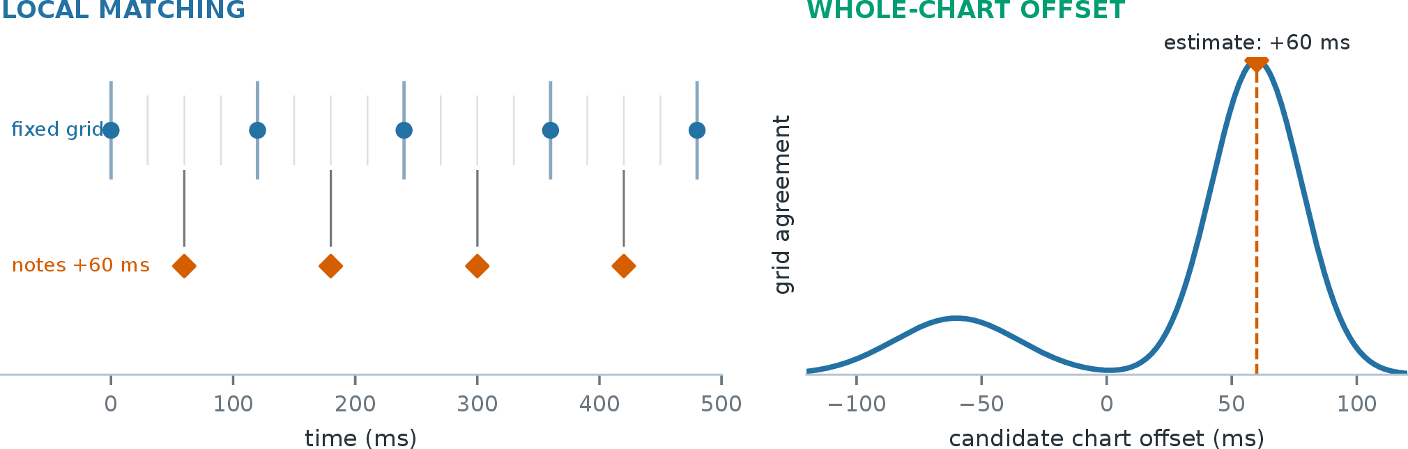
Nearest-grid matching can miss a constant shift (Figure 1). On a dense grid, each shifted note may simply be paired with another nearby grid point. We therefore estimate one offset for the whole chart. Let \(G_k\) be the fixed bar, beat, and eighth-note grids, and let \(d(x,G_k)=\min_{g\in G_k}|x-g|\). For note times \(t_i\), we score a candidate shift by \[\begin{align} S(\delta) &= \sum_k w_k\,\frac{1}{n}\sum_i \left[1-\frac{d(t_i-\delta,G_k)}{\tau}\right]_+,\\ \hat{\delta} &= \operatorname*{arg\,max}_{\delta\in[-250,250]\,\mathrm{ms}} S(\delta), \end{align} \label{eq:phase-offset}\tag{3}\] where \([z]_+=\max(z,0)\), \(\tau=12\) ms, and the bar, beat, and eighth-note weights are 0.2, 0.3, and 0.5. We search in 0.5 ms steps. Combining three grid levels reduces periodic ties. The resulting \(\hat{\delta}\) is a chart-level diagnostic: its magnitude says how far the chart must move to best align with the fixed musical-time framework. BPM alone provides a period but not a phase, so it cannot replace this anchor.
3.5 Controlled corruptions and acceptance rules↩︎
Starting from human charts, each corruption strengthens one operational failure. Other outputs may also move, so the tests establish target sensitivity rather than exclusive specificity. The target output and expected direction were fixed before the held-out run; all transformations appear in Appendix 9.
After orienting outputs so larger is better, support requires a negative dose-rank association, a negative strongest-dose contrast against the matched control, and every relevant invariance check to pass. We use song-cluster bootstrap intervals adjusted across ten prespecified rows. Full decision rules and sample accounting appear in Appendix 8.
4 Results↩︎
4.1 Core outputs respond to target failures↩︎
Every core output has the expected negative dose-rank association under its target failures (Table 2). The result covers nine nonredundant corruption–measurement pairs but seven output axes because the same 4-gram axis detects three distinct edits. All applicable invariance controls pass. The important result is not that every corruption needs a new metric. A small set of interpretable outputs can cover different failure mechanisms when each output is tested against a concrete claim.
| Targeted failure | Core output | Dose trend [99.5% CI] | Strongest-dose change [99.5% CI] |
|---|---|---|---|
| Dense timing jitter | timing clean rate | \(-.744\;[-.815,-.667]\) | \(-.502\;[-.558,-.446]\) |
| Sparse 60 ms timing errors | timing-error p99 | \(-.234\;[-.344,-.134]\) | \(-.306\;[-.508,-.144]\) ms |
| Whole-chart shift | grid-phase offset | \(-.916\;[-.981,-.826]\) | \(-55.58\;[-61.43,-49.83]\) ms |
| Note-type shuffle | transition familiarity | \(-.800\;[-.856,-.737]\) | \(-.231\;[-.262,-.199]\) |
| Loop collapse | 4-gram typicality | \(-.445\;[-.573,-.312]\) | \(-.165\;[-.226,-.108]\) |
| Common-pattern rewrite | 4-gram typicality | \(-.358\;[-.459,-.258]\) | \(-.131\;[-.189,-.078]\) |
| Note-rate scaling | note-rate typicality | \(-.693\;[-.784,-.579]\) | \(-.582\;[-.672,-.483]\) |
| Local burst insertion | density-spike limit | \(-.940\;[-.950,-.930]\) | \(-.619\;[-.644,-.593]\) |
| Bar-order shuffle | 4-gram typicality | \(-.589\;[-.728,-.435]\) | \(-.224\;[-.293,-.156]\) |
3.5pt
Sparse errors show why a tail statistic is needed when most notes remain correct. Complete sample counts and exclusions appear in Appendix 8.
4.2 External time detects chart–audio shifts↩︎
Translation symmetry predicts that a chart can look internally plausible yet be late relative to the song. The 40-song development experiment confirms this mechanism. After shifting every note by 15, 30, or 60 ms, no primary chart-only output changes by more than 0.03 human standard deviations. The phase estimator’s median matches each injected shift. With either the authored or audio-estimated grid, at least 169 of 170 charts are within 3 ms of the injected value.
Local matching and global phase answer different questions. A dense grid can re-pair a shifted note to another subdivision and still report a small local error. The whole-chart estimate preserves the shared offset instead. The same principle explains sparse failures: the mean remains dominated by correct notes, whereas timing-error p99 exposes the tail. Timing evaluation therefore needs both a song-side anchor and summaries at more than one scale.
4.3 Common proxies can reward the wrong behavior↩︎
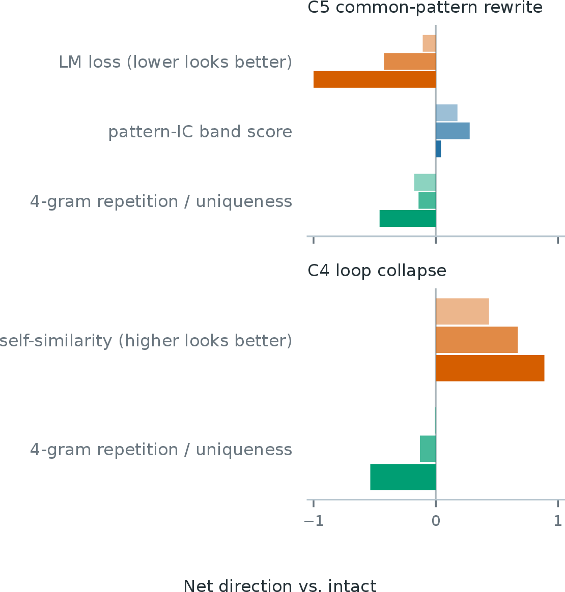
Two familiar proxies move in the wrong direction under targeted failures (Figure 2). LM perplexity rewards common-pattern rewriting: on the development panel, mean perplexity falls by 37%, from 9.44 to 5.98. A lower-is-better reading therefore prefers the corrupted chart, opposite to the intended property [16]. The reversal remains with a separately fitted scoring LM, while 4-gram typicality moves away from the human range. Secondary checks appear in Appendix 10.
If self-similarity is maximized as a quality objective, it rewards loop collapse. Repeating the dominant 4-gram raises mean self-similarity by 62% even though the note-type stream has collapsed into a four-event cycle [9]. 4-gram typicality moves in the opposite direction. The practical rule is to stress-test a candidate reward against the failure it is meant to prevent.
Automatic profiles shorten model-development feedback by identifying the failure mechanism that changed. Phase error and timing tails can guide minimization; density spikes provide a course-relative constraint; familiarity and typicality are soft targets or monitors. Optimization may use selected signals after task-specific stress testing, but no single number should become the reward.
5 Discussion↩︎
Typicality also needs context. A corruption often pushes a chart outside the same-course human band, but the reverse implication is invalid: an unusual chart may be deliberate and playable. Separate timing and feasibility checks help distinguish novelty from a concrete failure. When signals disagree, the disagreement is information rather than an error to hide with an average.
The descriptive public-system profiles in Appendix 10.3 illustrate two reusable reading habits. Similar clean-note fractions can hide different timing tails and global offsets, and a generator can match one difficulty while overshooting another. These examples are not additional metric validation; they show why diagnosis should follow failure mechanisms rather than one headline score.
6 Limitations↩︎
Controlled corruptions establish response to defined failures, not a universal ranking of chart quality. The present set does not cover every error, such as wrong-song pairing or removal of musically important notes. The response-to- music, long-form, and human-distance extensions were designed on the development panel and remain exploratory.
The human bands come from one Taiko corpus. Timing also requires an external grid; without an authored map or a reliable audio estimate, the timing outputs are unavailable. Finally, timing clean rate has no reference-note recall term, so deleting off-grid notes can improve it. This is why the profile reads clean rate together with note rate and keeps feasibility checks separate.
7 Conclusion↩︎
ChartGenEval turns chart evaluation into separate, testable feedback signals. Seven output axes pass nine held-out controlled-corruption tests. On the development panel, the song-anchored phase estimate recovers injected shifts invisible to chart-only statistics. Those development tests also show that likelihood and self-similarity can move in the wrong direction under targeted failures, so neither should be used alone as a quality score. The broader lesson is simple: automatic evaluation is most useful when each signal names a failure, survives a targeted stress test, and keeps its role visible to the model developer.
Ethics Statement↩︎
The study uses community-transcribed charts and associated audio gathered from online sources as described in Section 3.3; these potentially copyrighted materials are not redistributed. The released materials exclude source charts, audio, personal data, and generators. Automated evaluation can lower the cost of content production, so high-volume deployment still requires platform policy and moderation.
AI Usage Statement↩︎
AI assistants were used for experiment orchestration, drafting, and editing under author direction; the author checked all reported values.
8 Corpus Coverage and Held-Out Evaluation Protocol↩︎
8.1 Corpus coverage↩︎
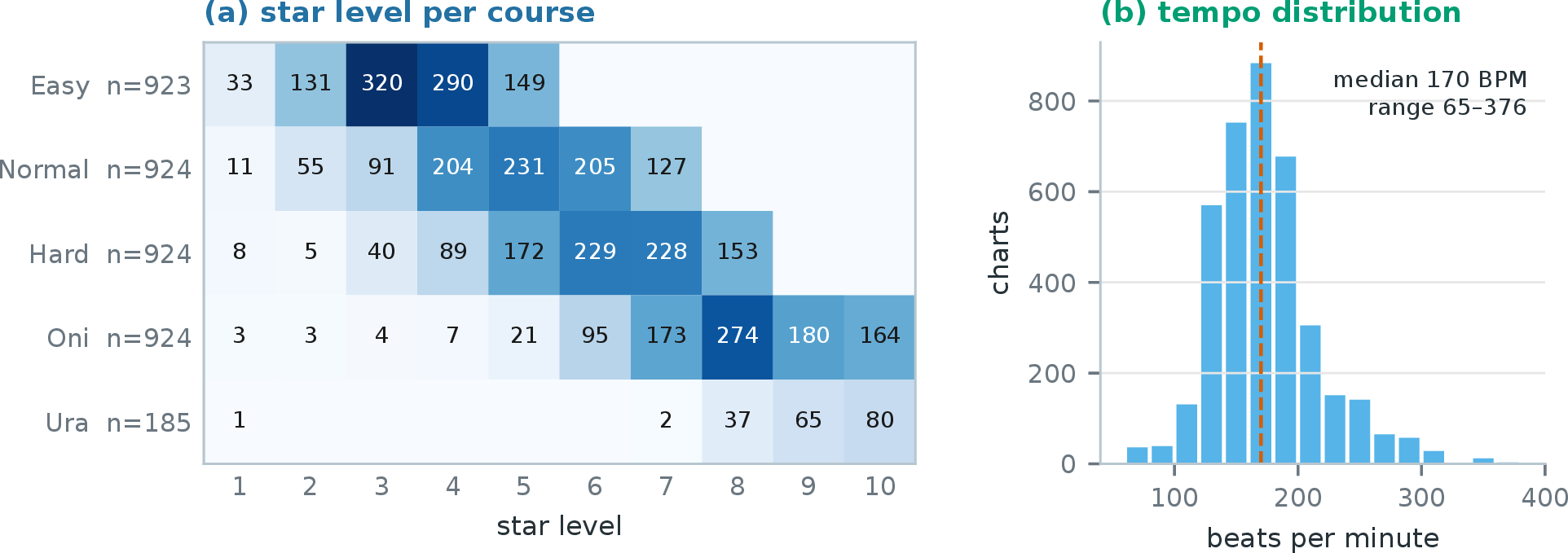
The calibration corpus is summarized by course, star level, and tempo. Figure 3 shows its difficulty and tempo coverage.
8.2 Corpus and timing details↩︎
We use Taiko-style chart files and associated audio gathered from community resources available online. The training split contains 924 source rows that resolve to 813 unique song groups and 3,880 course charts. The test split contains 140 source rows that resolve to 120 song groups. The underlying charts and audio may be copyrighted, so they are not redistributed.
The primary timing grid uses authored per-bar timestamps, meter, and tempo. For local timing diagnostics, every generated note is classified as within 6 ms, in the 6–12, 12–18, or above-18 ms range, or unmatched. We also compare adjacent intervals with tolerance \(\max(6\,\mathrm{ms},2.5\%\times\mathrm{IOI})\). An audio-downbeat estimate provides a development-stage alternative: its period is within 2% of the metadata period on 39 of 40 development songs and differs by 2.39% on the remaining song. Held-out absolute offsets use the authored grid because it fixes bar phase directly.
8.3 Panel construction and integrity↩︎
Source rows are canonicalized by group_id and audio SHA-256; inconsistent aliases are rejected before panel indexing. The test split contains 120 canonical song groups in stored order. Groups 0–39 form the development panel, and groups
40–119 form the held-out panel. Before inspecting held-out results, we fixed the dataset revision, corruptions and doses, target measurements, controls, thresholds, calibration, and analysis plan.
8.4 Replicates, completeness, and inferential units↩︎
Every nonzero corruption cell and control condition uses five fixed base seeds. Replicates are averaged within chart and dose. A course is complete only when its intact value, every target dose and replicate, matched control, and required checks are available. A song enters a test with at least one complete course, and complete courses are averaged within song. Songs, rather than charts, courses, or replicates, are the inferential units for both response statistics. Deterministic no-op and missing cells do not enter the analysis.
8.5 Control checks and numerical invariance↩︎
Identity re-evaluation applies to every retained measurement. A joint +1-second shift of notes, authored grid, and duration tests invariance to the time origin. A Don–Ka color bijection applies to timing and density, where color is irrelevant; it is not a grammar or form control. The 60 ms C2 translation is the matched control for chart-only density, grammar, and structure measurements. A required control failure prevents support for the affected target response. Each measurement uses a specified equivalence tolerance and timestamp-rounding rule. Chart-only interval arithmetic uses integer microseconds, three orders of magnitude finer than the smallest reported tolerance.
8.6 Intervals and decision rule↩︎
After orienting outputs so that larger is better, the first statistic is the within-chart Spearman correlation between the four severities (intact plus three doses) and the measurement; an all-constant response has zero sensitivity. The second statistic is the oriented maximum-dose value minus the matched control. Point estimates average song-level values. We use 10,000 song-cluster bootstrap draws: secondary analyses report nominal 95% intervals, and the ten primary rows use Bonferroni-adjusted 99.5% intervals. C6 assigns severities \([0,0.5,0.5,1]\) to the intact, \(0.5\times\), \(1.5\times\), and \(2\times\) conditions, so equal-magnitude low and high departures are tied; tied severities receive average ranks. A response is supported when at least 72 of 80 songs are evaluable, all controls pass, and both adjusted upper bounds are below zero. A nonnegative adjusted lower bound contradicts the response; other cases are inconclusive. The two C5 output rows were required to meet the rule together, although their algebraic equivalence leaves one effective axis. The C5 LM uses the full stored-order training split, trigram order 3, and add-\(\alpha=0.05\).
8.7 Sample counts and exclusions↩︎
The held-out execution produced 50,283 observation records from 333 charts. C1s retained 332 complete courses and C8 retained 330; every other effective pair retained 333. All 32 controls passed with maximum observed absolute difference zero. Nineteen deterministic no-op cells were excluded.
9 Controlled-Corruption Specifications↩︎
| Controlled corruption (strength) | Operational change | Prespecified response |
|---|---|---|
| C1 timing jitter (\(\pm\)10/20/30 ms) | all note times | timing clean rate \(\downarrow\) |
| C1s sparse timing errors (0.5/1/2%, \(\pm\)60 ms) | a few note times | timing-error p99 \(\uparrow\) |
| C2 whole-chart shift (+15/30/60 ms) | chart–song alignment | grid-phase offset \(\uparrow\) |
| C3 note-type shuffle (\(p{=}0.2/0.4/0.8\)) | local transitions | transition familiarity \(\downarrow\) |
| C4 loop collapse (\(p{=}0.3/0.6/1\)) | local repetition | 4-gram typicality \(\downarrow\) |
| C5 common-pattern rewrite (\(p{=}0.3/0.6/1\)) | pattern variety | 4-gram typicality \(\downarrow\) |
| C6 note-rate scaling (\(\times\)0.5/1.5/2) | difficulty fit | note-rate typicality \(\downarrow\) |
| C7 burst insertion (2/4/8 clusters) | local overload | density-spike limit \(\downarrow\) |
| C8 bar-order shuffle (\(p{=}0.3/0.6/1\)) | phrase order | 4-gram typicality \(\downarrow\) |
4pt
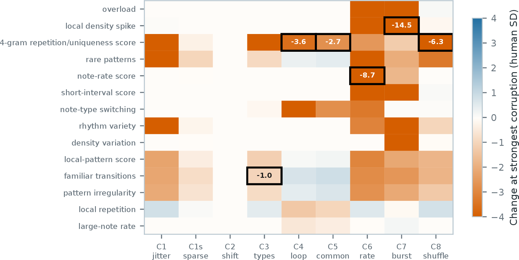
Figure 4 visualizes the operational change made by each corruption and its prespecified target measurement.
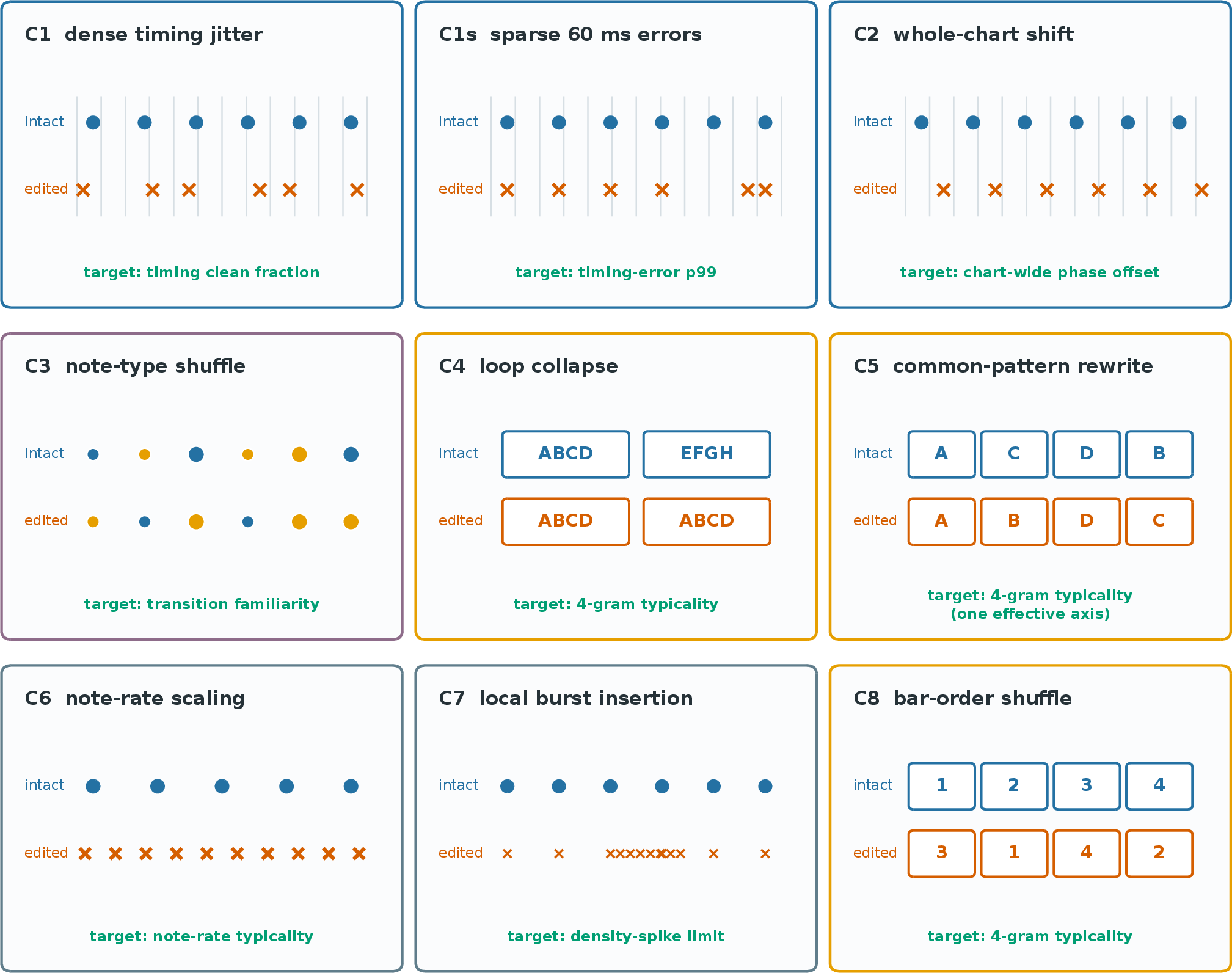
The 170-chart development matrix uses one realization per nonzero cell, producing 4,760 variants including the originals. C1s moves \(\max(1,\operatorname{round}(np))\) of a chart’s \(n\) notes by \(\pm60\) ms. C3–C5 preserve note times, while C4 and C6 preserve or control density. Raw features and their derived scores are evaluated on the same variants; equivalent quantities are counted once. For C5, one LM chooses common-pattern rewrites and a separately fitted LM scores them. The perplexity reversal remains (9.44 \(\to\) 6.04, \(-36\%\)).
10 Metric Guide and Extended Results↩︎
10.1 Exploratory measurements↩︎
Five additional components were selected or revised on the 40-song development panel. They remain useful hypotheses, but the main paper does not treat them as held-out-confirmed targets. Reciprocity compares two-bar phrases and rewards material that returns after an intervening phrase without rewarding adjacent copying. Stagnation–alienation marks active bars in long repeated runs or without a related bar within a 32-bar neighborhood. Density–energy response is the rank correlation between bar-level note density and mel energy. Run-head onset support asks whether the first note of a rhythmic group lies near strong spectral flux. Human-chart distance measures the mean distance to the 20 nearest same-course training charts in a standardized 32-feature representation.
Their development responses clarify their scope. Reciprocity reacts to loop collapse and bar shuffling; stagnation–alienation reacts most strongly to loop collapse. Run-head support detects whole-chart shifts, while density–energy response detects shuffled bars but is weak for short bursts. Human-chart distance detects many distributional departures but does not say whether an unusual chart is poor or creative. These outputs are therefore reported as exploratory monitors rather than core rewards.
10.2 Proxy diagnostics↩︎
The common-pattern rewrite is not an artifact of using the same LM for editing and scoring. When one LM selects the rewrite and a separately fitted LM scores it, perplexity still falls from 9.44 to 6.04 (\(-36\%\)). A symmetric band transform of LM loss also fails to identify the maximum rewrite dose: its held-out change is \(+0.021\) with a nominal 95% interval of \([-0.034,0.077]\). The 4-gram axis supplies the missing reading. Under loop collapse, set-level Self-BLEU rises from 0.845 to 0.898, also recording the loss of diversity.
Figure 5 connects each construct to its required inputs, representative outputs, and strongest present evidence. The evidence labels distinguish outputs with held-out corruption tests from components supported by development analyses.
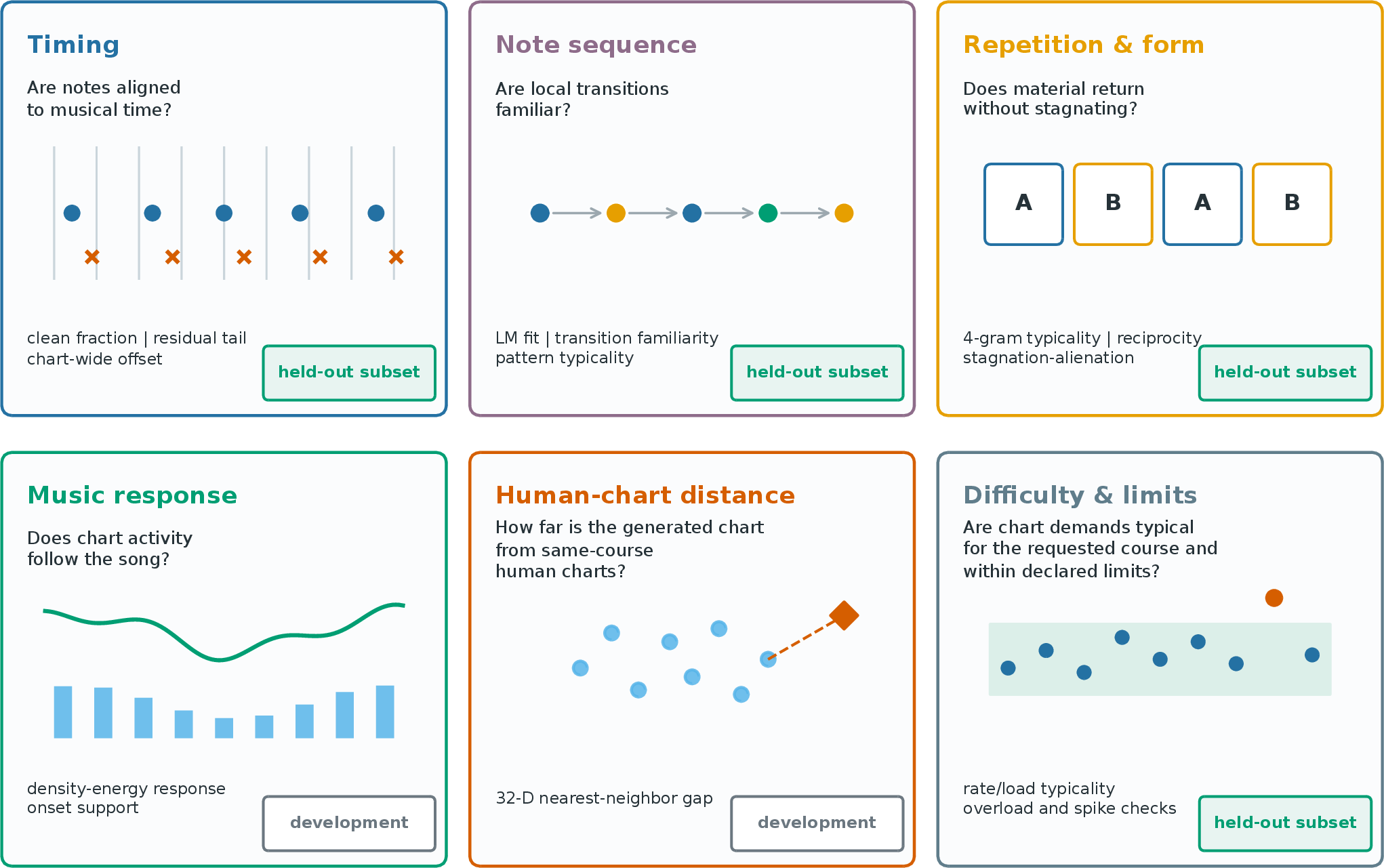
Figure 6 shows that targeted corruptions can affect multiple score families, motivating interpretation as a profile rather than as isolated interchangeable measurements.
10.3 Public-system profiles↩︎
We apply the profile to five public generators on the 40 development songs. Mapperatorinator v32 [17] and TaikoNation [2] produce Taiko note types. DDC’s onset pipeline [1], the public timing configuration of GenéLive! [3], and AutoOsu [18] enter only the applicable timing and audio-response readings. We use their public inference configurations without training or fine-tuning on this corpus. These profiles illustrate interpretation; they are not held-out metric tests or a generator leaderboard.
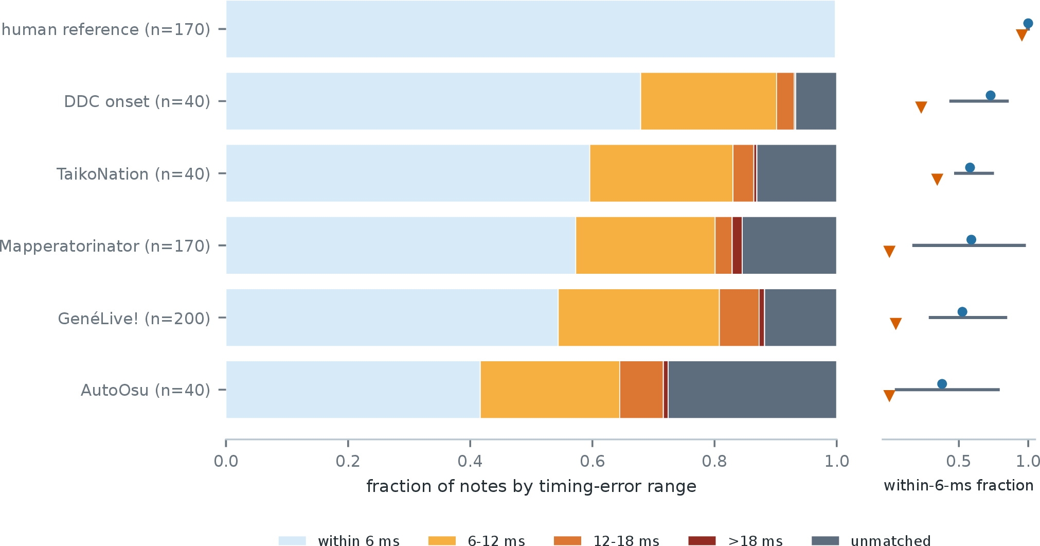
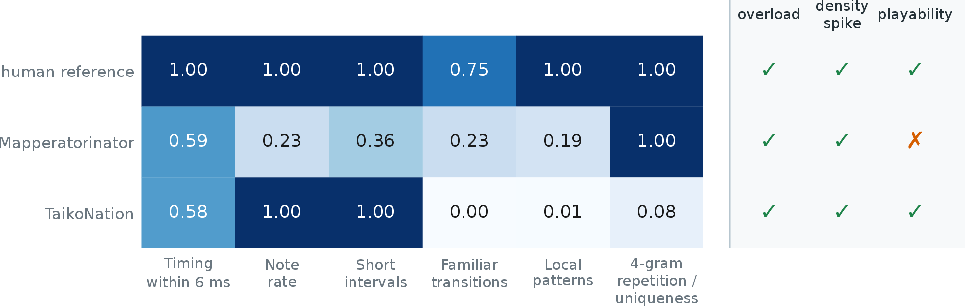
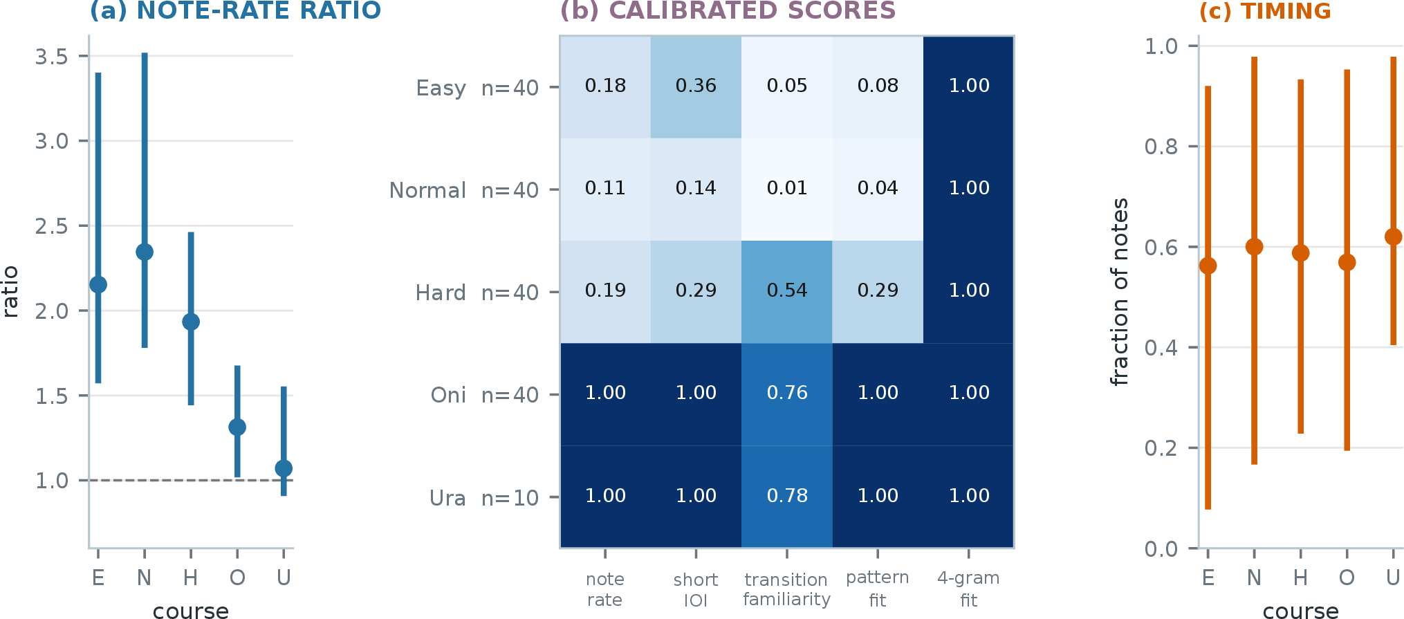
The two Taiko generators have similar median clean-note fractions, yet their relative-interval errors and global phase offsets differ. This is the same local-versus-global distinction exposed by the shift corruption. Difficulty conditioning reveals another pattern: Mapperatorinator overshoots human note rates most on easier courses, while its timing profile changes little by course. The useful conclusion is a course mismatch, not a general claim that the system improves at higher difficulty.
11 Released Materials↩︎
Code, evaluation records, and plotting scripts are available at https://github.com/JacobLinCool/ChartGenEval.