Visual Access Boundaries in
Vision-Language Model Reasoning
July 14, 2026
Abstract
Chain-of-Thought (CoT) prompting is widely used as a test-time scaling strategy for Vision-Language Models (VLMs), but it remains unclear what is extended when VLMs generate longer reasoning traces. We ask whether CoT requires continued access to image tokens, or whether it mainly operates over visual information already made available earlier in the forward pass. We introduce Visual Access Sweep, a causal intervention that masks attention from generated-token queries to image-token keys along layer depth and generation time, and define the Visual Access Boundary (VAB) as the minimal access region that preserves task accuracy. Across six model configurations from Qwen2.5-VL and InternVL3, both no-CoT direct answering and CoT prompting exhibit finite VABs. In Qwen2.5-VL-32B and InternVL3 at 14B and 38B scales, when CoT is evaluated against the no-CoT full-access target, its VAB layer differs from the no-CoT boundary by at most two layers, despite substantially longer generations. This suggests that CoT does not primarily improve performance by prolonging direct image-token access throughout the reasoning trace, but by extending language-side computation over image-derived hidden-state information. We further show that CoT gains are constrained by perceptual readout. CoT helps when the queried visual attribute can be reliably read out by the model, but not when that readout is unreliable. A symbolic-attribute oracle shows that CoT can improve counting once ground-truth attributes are supplied as text, while a single-object probe-vs-decode check shows that hard attributes can be linearly recoverable from hidden states yet difficult for the model itself to output. Together, these analyses place the bottleneck at readout rather than counting.
1 Introduction↩︎
CoT prompting is a standard test-time scaling tool in LLMs [1]–[3] and has also been adopted in VLMs [4]–[6]. However, its benefits on visual tasks are not uniform: some studies report gains from explicit intermediate reasoning, whereas others find limited or degraded gains on perception-heavy visual QA settings [7], [8]. What mechanism underlies CoT’s contribution to VLM performance? Does CoT improve performance by prolonging direct access to image tokens during generation, or by enabling additional language-side computation over visual information already made available earlier?
Existing evidence on this question is largely observational: studies document that VLM attention to image tokens decays as generation proceeds [9]–[13], but attention magnitude does not establish necessity. Low attention can mean that continued access is no longer used, or that access is failing; the two are indistinguishable from attention values alone. We therefore test necessity by intervention rather than by reading off attention.
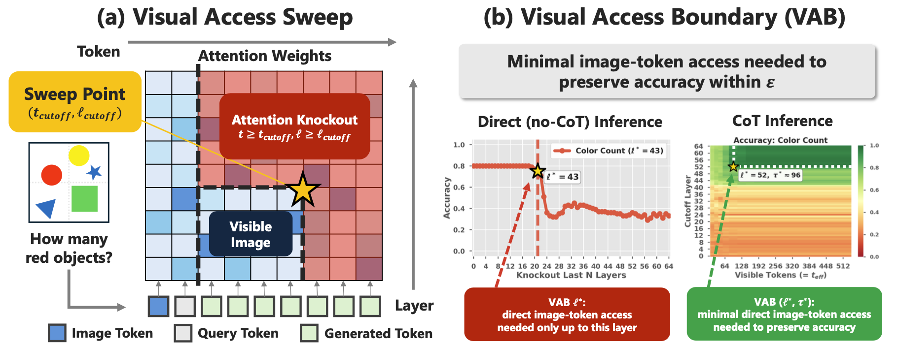
To answer this question, we introduce the Visual Access Boundary (VAB). We intervene by masking direct attention from generated-token queries to image-token keys across layer depth and generation time (Figure 1 (a)). We call this two-axis intervention Visual Access Sweep. This intervention turns an otherwise observational question into a causal one. If performance is preserved after removing later generated-token access to image tokens, then those direct visual accesses are not necessary for the target behavior. Instead, when CoT helps, it appears to operate over image-derived information already carried in hidden states.
To isolate visual grounding from downstream reasoning, we design controlled attribute-counting tasks in which object attributes and spatial layouts are fully parameterized, following the spirit of controlled visual reasoning benchmarks. This avoids cases where a model can answer from parametric knowledge or dataset bias rather than from the image itself, while keeping the reasoning operation fixed as counting and varying only the queried visual attribute. We compare no-CoT direct answering, which we refer to as Direct, with CoT prompting. We further test whether the same structure appears beyond synthetic images using a GQA-derived real-image yes/no task [14].
Applied across six model configurations from Qwen2.5-VL and InternVL3, Visual Access Sweep yields two main findings. First, as schematized in Figure 1 (b), a Visual Access Boundary exists clearly under both Direct and CoT prompting. In every main model-task setting we test, accuracy is preserved while a broad upper-layer region is blocked, then drops sharply once the intervention reaches earlier layers. Taken together, these results adjudicate between the two mechanisms above. In Direct answering, there is a depth after which generated tokens no longer need direct attention to image tokens. Under CoT, generation becomes much longer, but the necessary visual-access region does not expand proportionally along the generation-time axis. Thus, in the regimes we test, CoT does not primarily improve performance by continuing to re-read the image throughout the reasoning trace. Instead, when CoT helps, it appears to operate over image-derived information already carried in hidden states. The same qualitative VAB structure also appears on the GQA-derived real-image task. Second, on Qwen2.5-VL across three scales, per-attribute CoT gains are predicted by multi-object perceptual readout accuracy at 3B and 7B and saturate at 32B. An oracle bypass that supplies the attribute symbolically restores CoT gains uniformly across attributes, and a probe-vs-decode gap on hard attributes provides separate single-object evidence that the bottleneck sits at perceptual readout rather than the counting operation itself (Section 6).
Our contributions are as follows. (i) We introduce Visual Access Sweep and the Visual Access Boundary, a causal intervention and an operational measure that together map the functional necessity of direct image-token access along both layer depth and generation time. (ii) We show that finite VABs appear under both Direct and CoT prompting across the main Qwen2.5-VL and InternVL3 settings. In larger models, the CoT VAB layer remains within two layers of the no-CoT boundary when evaluated against the no-CoT full-access target, despite much longer generations. The same qualitative VAB structure also appears on a GQA-derived real-image yes/no task. (iii) On Qwen2.5-VL, per-attribute CoT gain tracks multi-object perceptual readout accuracy across three scales and is restored uniformly by an oracle bypass on the same checkpoint without image input. A separate single-object probe-vs-decode diagnostic on hard attributes provides supporting evidence that the bottleneck sits at perceptual readout rather than the counting operation itself.
2 Related Work↩︎
2.0.0.1 Visual attention decay in VLMs.
A growing body of work shows that VLM attention to image tokens often weakens, becomes noisy, or is misallocated during generation, and several methods improve performance by strengthening, redistributing, or re-injecting visual signals during inference [9]–[13]. These studies establish that modifying visual attention can be beneficial. Our question is complementary. In an unmodified prefix-based decoder-only VLM, when is continued direct image-token access functionally necessary during generation? Rather than enhancing visual attention, Visual Access Sweep removes generated-token access to image tokens along layer depth and generation time, thereby testing necessity rather than utility of attention amplification.
2.0.0.2 CoT and test-time scaling in VLMs.
CoT and test-time scaling are well established in LLMs [1]–[3], [15] and have been extended to VLMs, with some studies reporting improved multimodal reasoning [4]–[6], [16] and others showing limited or degraded gains in perception-heavy settings [7], [8]. Rather than searching for the best prompting recipe, we ask what is being extended when CoT does help. Because generated rationales need not faithfully reveal the computation that produced the answer [17], [18], we do not infer visual use from the CoT text itself; we instead test the functional necessity of image-token access by intervention.
2.0.0.3 Active perception and visual re-access.
Several recent approaches modify VLM inference by allowing the model to acquire additional visual evidence during reasoning, for example through visual memory, region refocusing, or explicit perception actions [19]–[21]. These methods study how to improve models by adding a perception-reasoning feedback loop. Our work asks a complementary diagnostic question. We test whether ordinary CoT already makes continued direct access from generated tokens to the initial image-token prefix functionally necessary in prefix-based decoder-only VLMs.
2.0.0.4 Mechanistic interpretability and probing in VLMs.
Causal-intervention methods on attention or activations [22]–[26] and probing studies showing VLM hidden states encode visual information the model fails to verbalize [27]–[31] both inform our approach. Unlike tuned-lens-style observational decoding, the VAB measures via causal masking where direct image-token access stops being necessary, and we go beyond generic readout-bottleneck observations by relating the probe-vs-decode gap to CoT gain through oracle bypass.
3 Experimental Design↩︎
3.1 VLM formulation↩︎
We focus on decoder-only VLMs in which a frozen vision encoder followed by a projection layer produces image tokens that are concatenated as a prefix to text tokens, and outputs are generated autoregressively [32]–[36]. Throughout this paper, when we refer to attention from generated-token queries to image-token keys, we mean the corresponding entries of the standard self-attention matrix in this prefix-based decoder-only setup, rather than a separate cross-attention module. Let \(\mathbf{t}_{\mathrm{img}} = (t_{\mathrm{img},1}, \ldots, t_{\mathrm{img},K})\) denote the \(K\) image tokens, \(\mathbf{t}_{\mathrm{text}}\) the input text tokens, and \(\mathbf{t}_{\mathrm{gen},1:t-1}\) the previously generated tokens; at step \(t\) the model conditions on \(\mathbf{T}_t = [\mathbf{t}_{\mathrm{img}},\, \mathbf{t}_{\mathrm{text}},\, \mathbf{t}_{\mathrm{gen},1:t-1}]\) and predicts \(t_{\mathrm{gen},t}\). The operational definition of visual access that our intervention manipulates is given in Section 4.1.
3.2 Tasks and datasets↩︎
We use two task families, a controlled synthetic attribute-counting task family that allows precise factor isolation and a real-image scene-graph QA task derived from GQA that probes external validity beyond synthetic stimuli.
3.2.0.1 Controlled attribute-counting tasks.

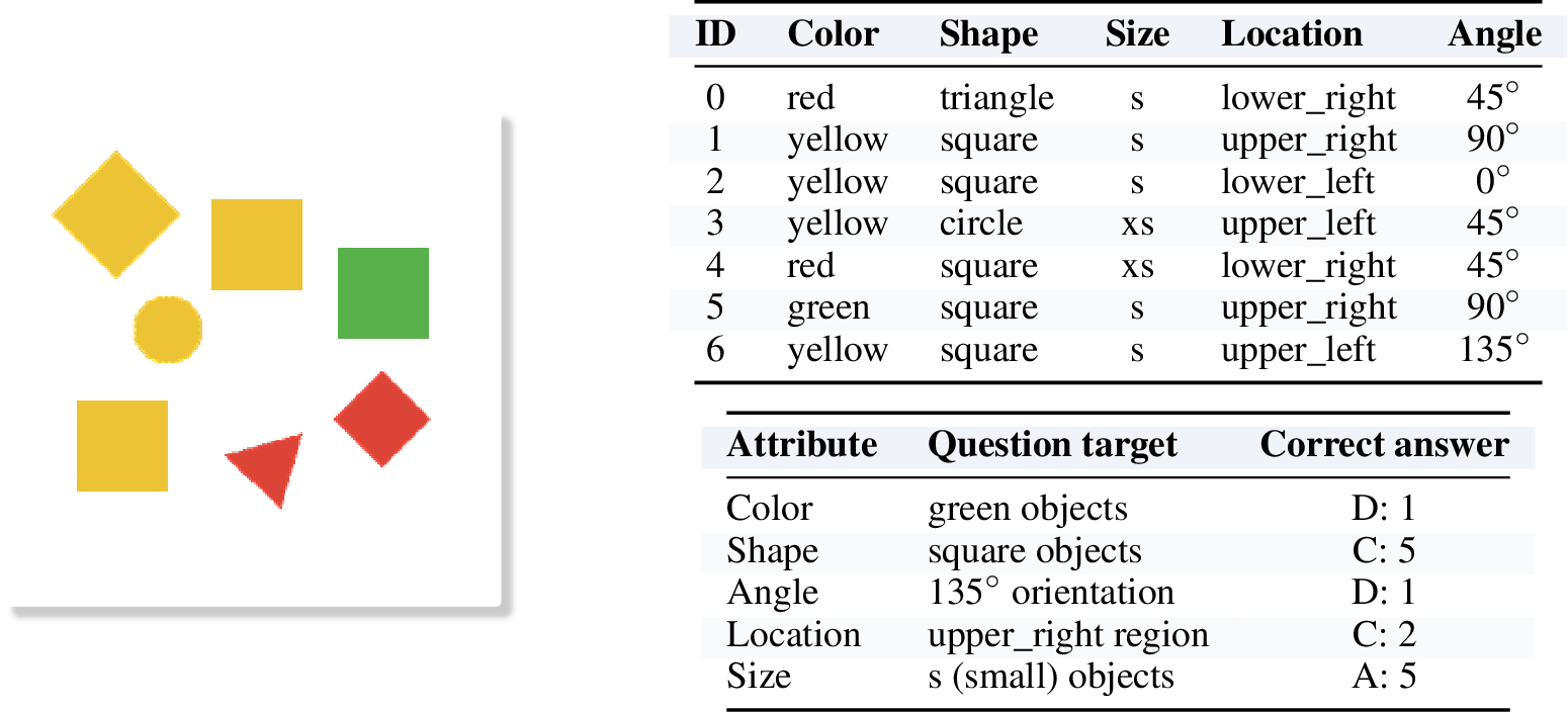
The controlled tasks vary the queried visual attribute while holding the reasoning operation fixed (counting). Each scene is procedurally generated with parameterized objects whose attributes (color, shape, location, angle, size, with 4 classes each) span a range of perceptual difficulty (Appendix 8.1). For each scene we issue five counting queries of the form “How many attribute=value objects are in the image?” (Figure 2), one per attribute.
The role of these tasks is diagnostic, not benchmark coverage. Holding the reasoning operation fixed across attributes makes it harder to attribute differences in CoT gain to differences in reasoning difficulty. What varies is the difficulty of obtaining the relevant attribute in a form usable by counting. Section 6 uses two diagnostics on the same attributes, namely multi-object readout on the counting scenes and a single-object probe-vs-decode check in Appendix 11.1. Both test whether the queried attribute is available as a usable symbol. A concrete counting example is in Appendix 8.2.
3.2.0.2 Real-image scene-graph QA.
To test whether the VAB structure is specific to synthetic stimuli, we additionally construct a real-image extension from the balanced validation split of GQA [14].1 GQA contains natural photographs paired with scene-graph-derived questions, and its balanced split is designed to reduce answer-distribution bias. We use the yes/no subset to keep the answer space controlled and to reduce answer-parsing ambiguity. Full preprocessing, prompting, answer extraction, and license details are in Appendix 10.6.
For both task families, we compare Direct prompting, which asks for a final answer with minimal intermediate output, against CoT prompting, which asks the model to produce intermediate reasoning before the final answer. Controlled counting is evaluated by constrained option-key accuracy, and the GQA-derived task by binary yes/no accuracy. Full prompt templates, answer extraction rules, decoding settings, and compute details are provided in Appendix 8.3 and Appendix 8.4.
4 Visual Access Sweep↩︎
4.1 Intervention↩︎
We operationally define visual access at \((\ell, t)\) as direct attention from the generated-token query at generation step \(t\) and layer \(\ell\) to image-token keys (Figure 1 (a)). Visual Access Sweep restricts this channel by two cutoffs. Image-token access is allowed only inside the rectangle \(\ell \le \ell_{\text{cutoff}}\) and \(t \le t_{\text{cutoff}}\), and is masked outside this region. Sweeping \((\ell_{\text{cutoff}}, t_{\text{cutoff}})\) thus traces how much direct image-token access is needed to preserve task performance.
Throughout this paper, visual access denotes this specific computational channel. Visual information that has already been incorporated into hidden states through earlier computation can still persist through the residual stream and is not removed by this intervention. Concretely, for the additive attention mask \(\mathbf{M}^\ell\) at layer \(\ell\), we set \(\mathbf{M}^\ell_{ij} = -\infty\) for every (generated-query position \(i\), image-token key position \(j\)) pair within the masked region, so that the corresponding post-softmax attention weight is exactly zero: \[\mathrm{Attention}(\mathbf{Q}^\ell, \mathbf{K}^\ell, \mathbf{V}^\ell) = \mathrm{softmax}\!\left( \frac{\mathbf{Q}^\ell {\mathbf{K}^\ell}^\top}{\sqrt{d}} + \mathbf{M}^\ell \right) \mathbf{V}^\ell, \; \mathbf{M}^\ell_{ij} = \begin{cases} -\infty & \text{if intervention active}, \\ 0 & \text{otherwise}. \end{cases}\] The layer cutoff \(\ell_{\text{cutoff}}\) keeps direct image-token access in layers \(1, \ldots, \ell_{\text{cutoff}}\) and removes it in all subsequent layers. The token cutoff \(t_{\text{cutoff}}\) keeps access for the first \(t_{\text{cutoff}}\) generated tokens and removes it thereafter. Because direct prompting and CoT prompting produce sequences of very different lengths, we use the effective window \(t_{\text{eff}} = \min(t_{\text{cutoff}}, T_{\text{gen}})\) and treat samples with \(T_{\text{gen}} < t_{\text{cutoff}}\) as having full token-axis access. The full-access baseline corresponds to the sweep point with the largest layer and token cutoffs. To verify that the observed boundary is not an artifact of the masking operation, Appendix 9.1 reports null-sink and late-layer query-text-block controls. These controls test for attention redistribution and query-mediated re-reading, respectively, and both preserve the qualitative VAB structure on Qwen2.5-VL-32B.
4.2 Visual Access Boundary↩︎
Figure 1 (b) illustrates how the sweep is read. If accuracy remains within tolerance after masking a broad late-layer or late-token region, then continued direct image-token access in that region is not functionally necessary for the task.
For compact notation, we write \(\tau\) for the effective token window \(t_{\text{eff}}\). Let \(A^{p}_{\mathrm{full}}\) denote the full-access accuracy under prompt condition \(p \in \{\mathrm{D}, \mathrm{CoT}\}\), and let \(A^{p}(\ell, \tau)\) denote the accuracy after applying the visual-access cutoff \((\ell, \tau)\) under the same prompt condition.
For a tolerance \(\epsilon\), each boundary is defined as the minimal access region on the sweep grid whose criterion-specific accuracy drop is at most \(\epsilon\). We use \(\epsilon = 0.05\) throughout, corresponding to a 5-percentage-point accuracy budget. The three drops we compare against \(\epsilon\) are \[\begin{align} \Delta_{\mathrm{D}}(\ell, \tau) &= A^{\mathrm{D}}_{\mathrm{full}} - A^{\mathrm{D}}(\ell, \tau), \\ \Delta_{\mathrm{CoT}}(\ell, \tau) &= A^{\mathrm{CoT}}_{\mathrm{full}} - A^{\mathrm{CoT}}(\ell, \tau), \\ \Delta_{\mathrm{DA}}(\ell, \tau) &= A^{\mathrm{D}}_{\mathrm{full}} - A^{\mathrm{CoT}}(\ell, \tau). \end{align} \label{eq:vab-criteria}\tag{1}\] The Direct boundary \(\ell^*_{\mathrm{D}}\) is computed from \(\Delta_{\mathrm{D}}\). The CoT-own-max boundary \(\ell^*_{\mathrm{CoT}}\) is computed from \(\Delta_{\mathrm{CoT}}\), asking when CoT under intervention preserves CoT’s own full-access ceiling. The direct-anchored CoT boundary \(\ell^*_{\mathrm{DA}}\) is computed from \(\Delta_{\mathrm{DA}}\), asking when CoT under intervention reaches the Direct full-access target.
We report two layer shifts, \[\Delta\ell^*_{\mathrm{own}} = \ell^*_{\mathrm{CoT}} - \ell^*_{\mathrm{D}}, \qquad \Delta\ell^*_{\mathrm{DA}} = \ell^*_{\mathrm{DA}} - \ell^*_{\mathrm{D}}. \label{eq:vab-layer-shifts}\tag{2}\] Per-setting numbers are summarized in Section 5.2 and reported in Appendix 10.1. We verify in Appendix 9.2 that the central CoT-vs-Direct comparison is stable under \(\epsilon \in \{0.03, 0.05, 0.07, 0.10\}\) (\(|\Delta\ell^*_{\mathrm{DA}}| \le 1\) under the direct-anchored criterion at all \(\epsilon\) tested). By construction, the VAB measures the functional necessity of continued direct image-token access. It does not erase image-derived information that has already propagated into hidden states.
5 Visual Access Boundary in Direct and CoT Inference↩︎
Across model families, scales, and stimulus domains, Visual Access Sweep reveals a consistent structure. Performance is preserved after masking a broad late region of direct image-token access, and drops sharply only when the intervention reaches earlier layers or earlier generated tokens. This structure appears in Direct inference, persists under CoT prompting, and also appears on a GQA-derived real-image QA task. The main empirical result is therefore not a particular numerical layer shift, but the repeated emergence of a finite Visual Access Boundary. Extended generation does not imply continued direct image-token access throughout the reasoning trace.
5.1 Visual Access Boundary in direct inference↩︎
We first establish that direct inference exhibits a clear functional boundary on continued image-token access. Figure 3 (a) shows the Direct layer sweep on Qwen2.5-VL-32B for color and shape counting. Accuracy remains near the full-access baseline while a broad upper-layer region is blocked, then drops sharply once the intervention reaches earlier layers. Exact \(\ell^*\) values are reported in the figure and in Appendix 10.1. We interpret this boundary operationally. Beyond \(\ell^*\), additional direct attention from generated tokens to image tokens is no longer needed for this task, although visual information already carried in hidden states may still be used.
5.2 Visual Access Boundary in CoT inference↩︎
We now ask whether the much longer generation produced by CoT requires a correspondingly larger region of direct image-token access. Figure 3 (b) shows the joint sweep over layer and effective token cutoffs under CoT on Qwen2.5-VL-32B. The region where \(\Delta_{\mathrm{CoT}}(\ell, \tau) \le \epsilon = 0.05\) occupies the upper portion of the heatmap, and the star marks the empirical \((\ell^*, \tau^*)\).
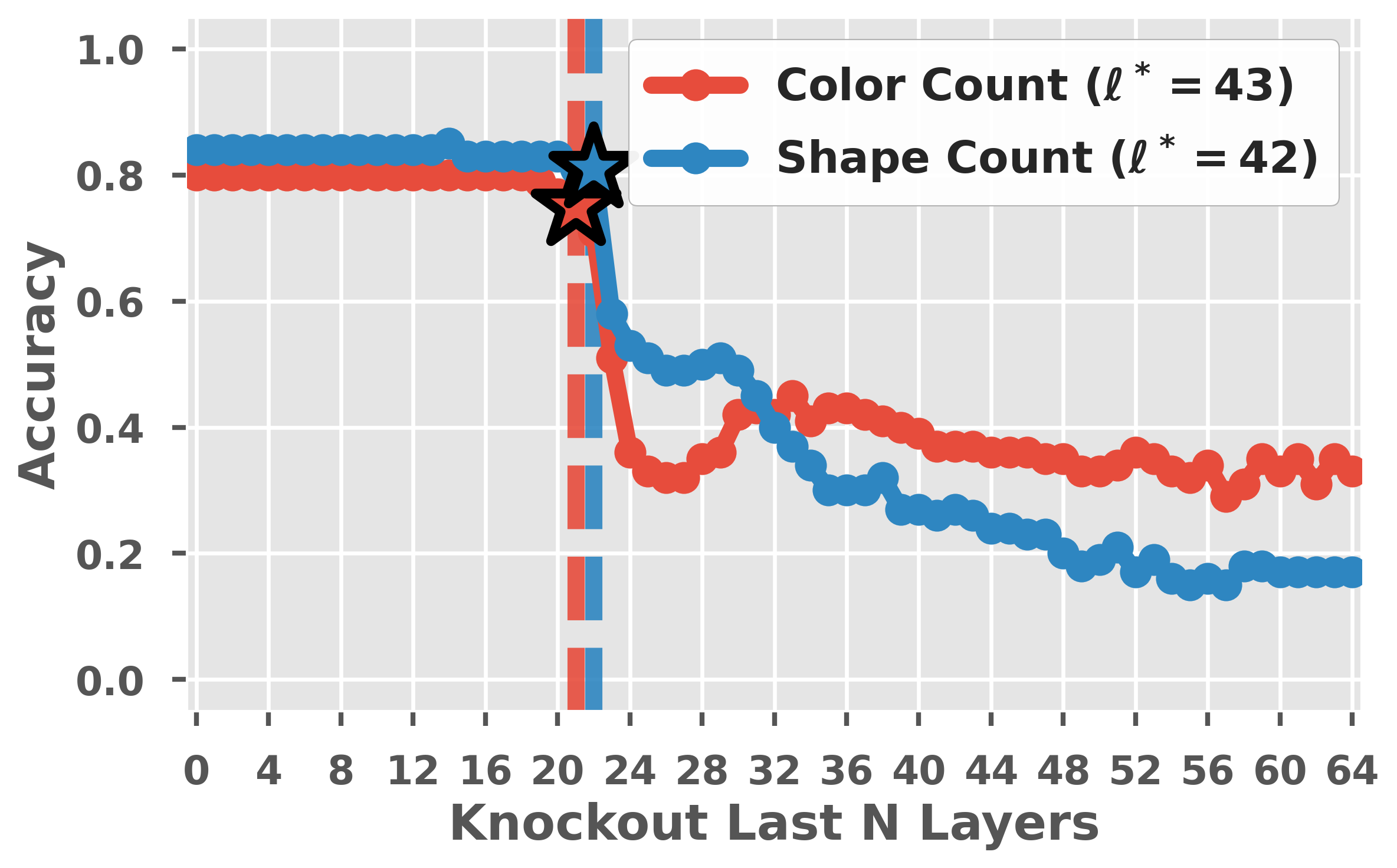
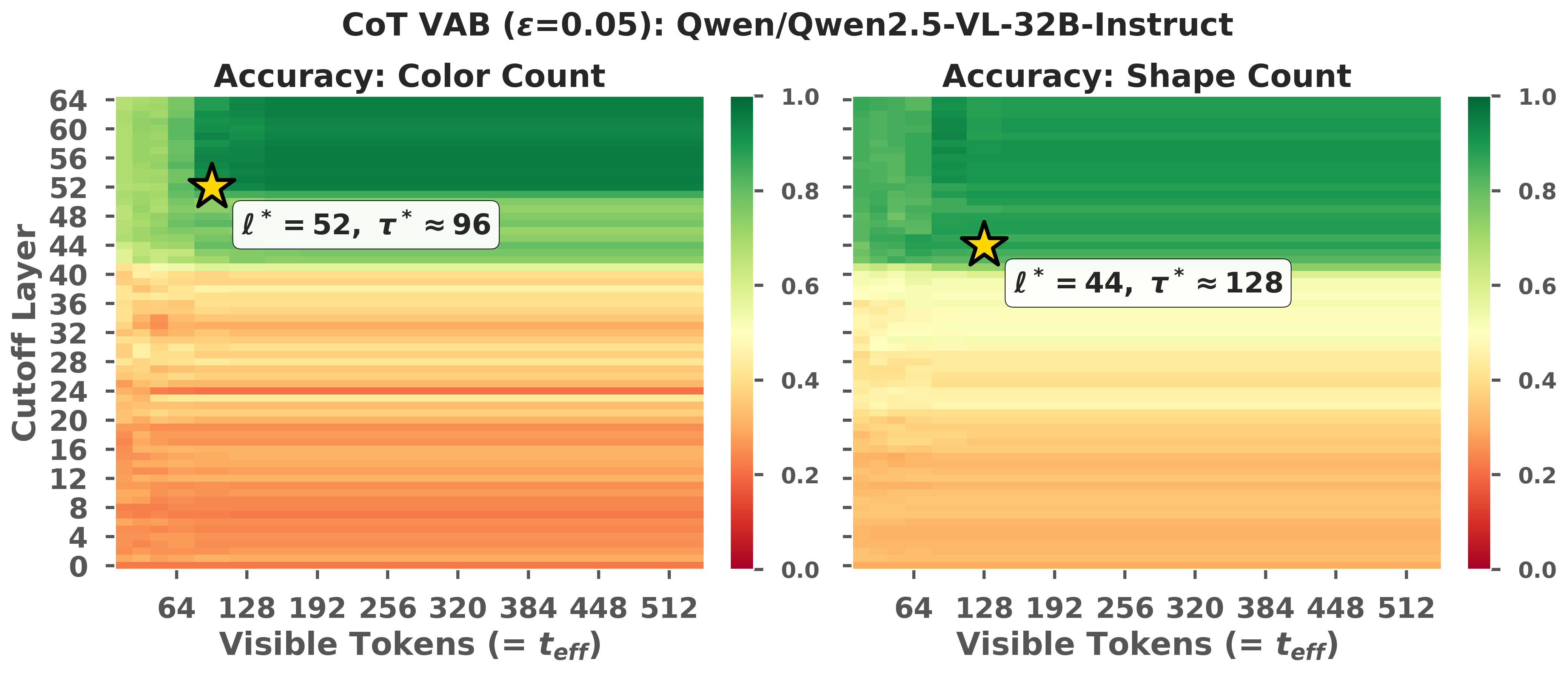
Figure 3: Visual Access Boundary on Qwen2.5-VL-32B. (a) Direct inference shows a sharp layer-wise transition: accuracy is preserved while a broad upper-layer region is blocked, but drops once the intervention reaches earlier layers. (b) Under CoT, the high-accuracy region remains concentrated in a similar depth range despite much longer generations. Stars mark the empirical VAB under \(\epsilon = 0.05\). Exact boundary values are reported in Appendix 10.1.. a — Direct: layer sweep for color and shape counting., b — CoT: layer-token sweep. Stars mark the empirical \((\ell^*, \tau^*)\).
We use the CoT-own-max and direct-anchored criteria defined in Section 4.2. The structural observation is that, across the 12 (family, scale, task) settings we test, \(|\Delta\ell^*_{\mathrm{own}}|\) stays within 9 layers while generation length increases by approximately \(50\times\). The direct-anchored CoT boundary is generally close to the Direct VAB on the larger models for which the target is attainable (Qwen2.5-VL-32B and the 14B and 38B variants of InternVL3 yield \(|\Delta\ell^*_{\mathrm{DA}}| \le 2\)). Settings where the direct-anchored target is not reached are reported separately. The consistent pattern is the existence of a finite VAB under CoT, not a monotonic deepening of the boundary. We discuss possible mechanisms for this decoupling in Section 7.
5.3 Cross-family and cross-scale VAB sweeps↩︎
A natural concern is that the VAB structure could be specific to a single family, since differences in vision encoder, projection, and training data could in principle create an architecture-specific late-layer redundancy. We evaluate the same Visual Access Sweep on Qwen2.5-VL [36] at three scales (3B, 7B, 32B) and on InternVL3 [37] at three scales (8B, 14B, 38B). A layer-wise VAB is observed in every case (per-model figures in Appendix 10.4, architectural details in Appendix 10.2). The shift is not consistently positive. Qwen2.5-VL scales tend to show non-negative CoT-own-max shifts, whereas InternVL3 does not show a systematic deepening. In some larger InternVL3 settings, the CoT boundary is comparable to or slightly shallower than the Direct boundary. What is constant across architectures is therefore the absence of generation-proportional expansion, not a single-direction shift.
5.3.0.1 Cross-attention fusion architectures.
We further apply the same intervention principle to a cross-attention-based VLM (Llama-3.2-11B-Vision-Instruct [38]), where visual access is implemented by masking the generated-token queries’ cross-attention to visual keys rather than self-attention to an image-token prefix (Appendix 10.5). The CoT-side sweep again exhibits a finite VAB. This pilot check suggests that the intervention principle can be applied beyond prefix-fusion models, with explicit iterative re-perception modules remaining the main untested regime.
5.4 Real-image scene-graph QA extension↩︎
A second concern is that the VAB structure might be a property of the synthetic CLEVR-style stimuli [39] rather than of decoder-only VLMs. We apply Visual Access Sweep to the GQA-derived real-image scene-graph QA task on Qwen2.5-VL-32B (Section 3.2.0.2). At full access, Direct accuracy is \(0.84\) and CoT accuracy is \(0.80\) (Appendix 10.6). Figure 4 shows the joint sweep for both prompting modes.
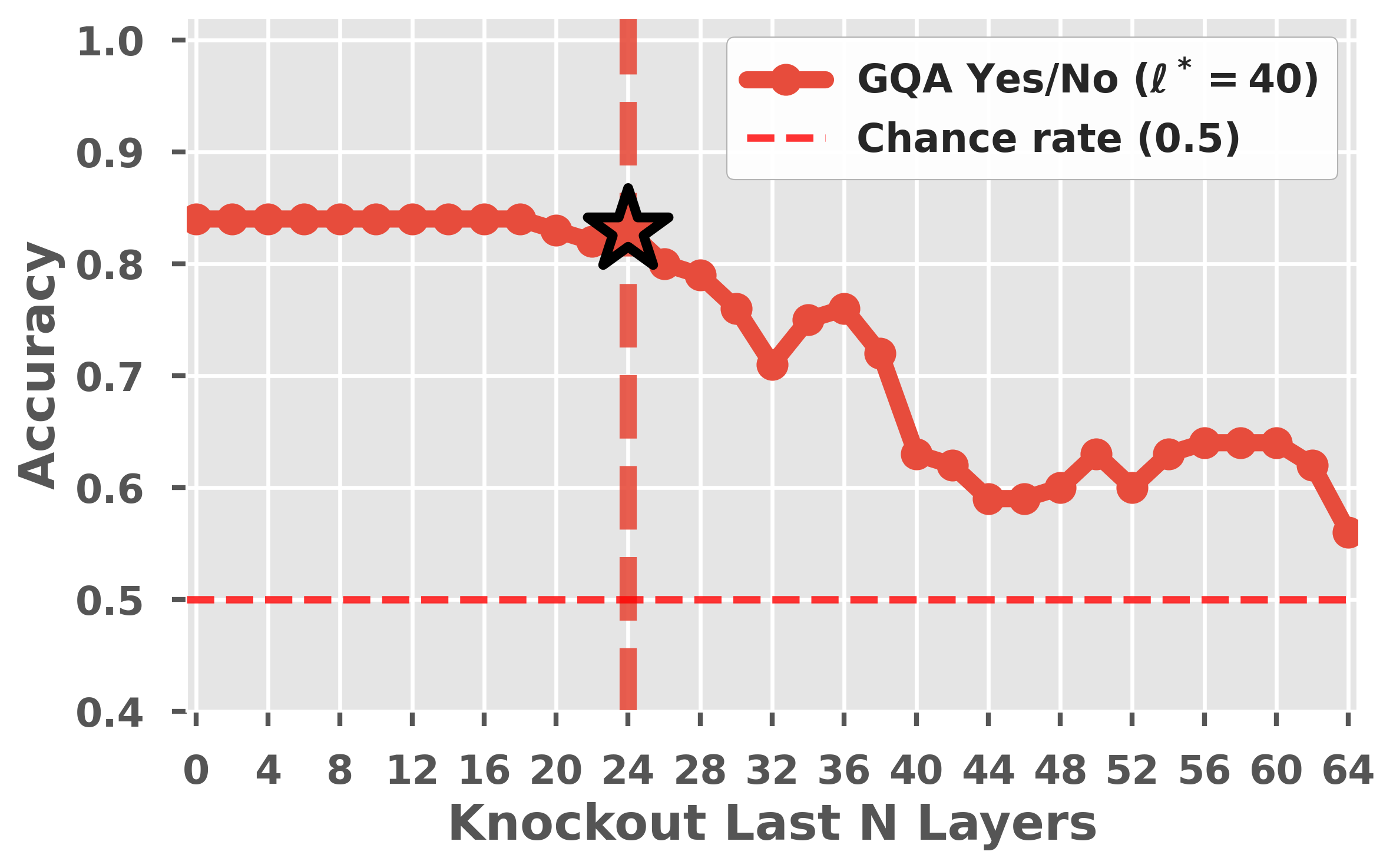
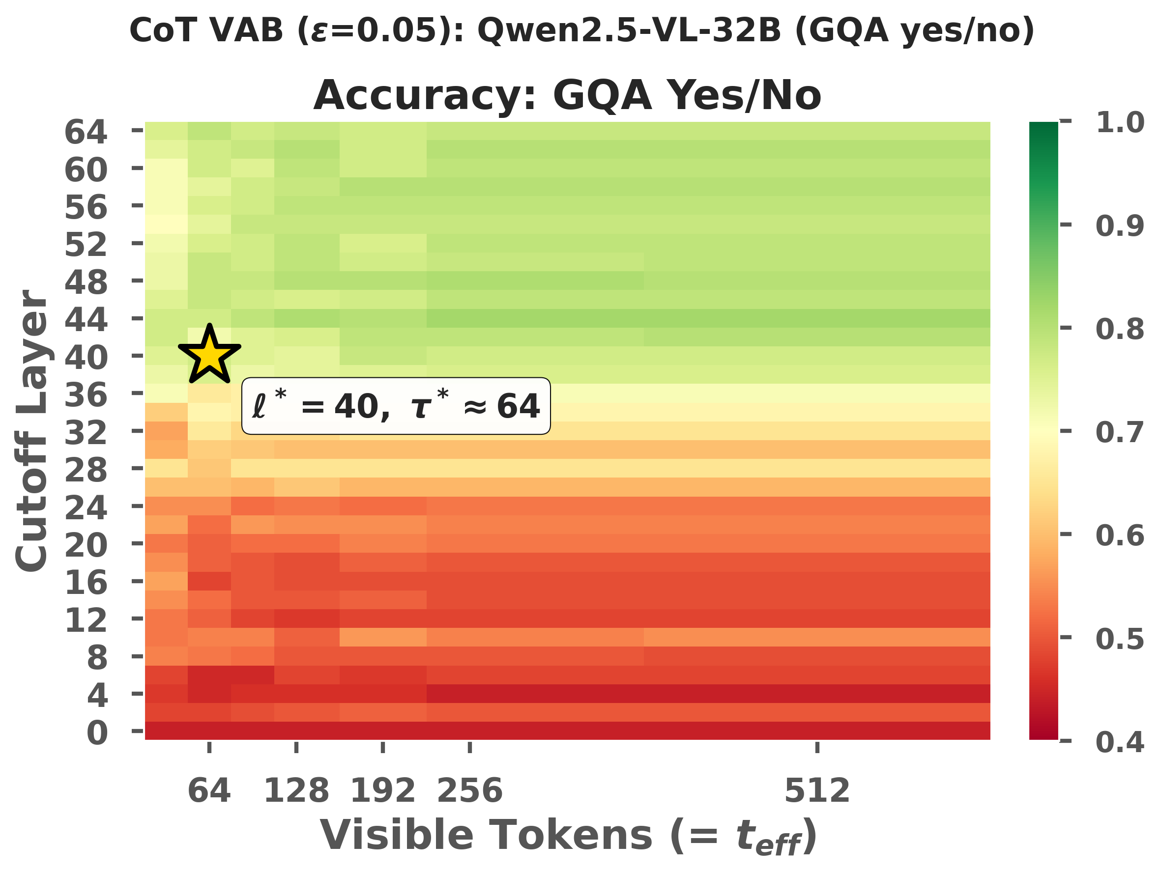
Figure 4: Real-image extension: VAB on GQA yes/no (Qwen2.5-VL-32B). (a) Direct inference reproduces the qualitative pattern of the controlled tasks. A broad upper-layer region can be blocked with little accuracy loss before a sharp transition. (b) Under CoT, the high-accuracy region is concentrated within a similar depth range despite much longer generations. Both prompting modes therefore exhibit a finite VAB on real images. Exact boundary values are reported in Appendix 10.6.. a — Direct: layer sweep on GQA yes/no., b — CoT: layer-token sweep. Star marks \((\ell^*, \tau^*)\).
Although CoT does not improve this binary GQA setting, this aligns with recent evidence that longer reasoning in VLMs can weaken perceptual grounding rather than monotonically improve visual QA [40], [41]. Both Direct and CoT sweeps still exhibit a finite VAB, with the redundant late-layer region comparable in size to synthetic counting on the same model. The GQA result thus extends the VAB phenomenon to real images while separating the existence of a visual-access boundary from whether CoT improves final accuracy.
6 Perceptual Readout Restricts CoT Gains↩︎
The Visual Access Sweep results say that, in the regime we study, CoT gains do not come from extending direct image-token access. They do not yet say what determines whether CoT gains exist at all on a given task. In this section, we show that within Qwen2.5-VL, the magnitude of CoT gains is constrained by whether the queried visual attribute can be read out into a form usable by the model’s own reasoning chain.
6.1 Defining perceptual readout↩︎
We distinguish two questions. The first is whether an attribute is encoded somewhere in the model’s hidden states. The second is whether the model can turn that attribute into a symbol that its own answer-generation process can use. This section focuses on the second question.
We use two related readout diagnostics. The main predictor of CoT gain is a multi-object perceptual readout task, in which the model is given a scene with multiple objects and must fill in the queried attribute value for every object, while the remaining attributes are provided as textual scaffolding. We use this multi-object perceptual readout accuracy as the x-axis in Figure 5. Separately, Appendix 11.1 reports a single-object probe-vs-decode diagnostic, which tests whether attribute information is linearly decodable from hidden states even when the model cannot reliably express it in its own output. Neither is a parallel main task. Both are evaluation devices for whether the queried visual attribute is available as a usable symbol.
This distinction is necessary because latent encoding and decoded availability can diverge. On Qwen2.5-VL-32B, hard attributes such as angle, location, and size show large probe-vs-decode gaps. A linear probe on hidden states recovers them with high accuracy while the model’s own direct decoding is substantially lower (Appendix 11.1, Table ¿tbl:tab:s1-probing-decoding?). The bottleneck is therefore not whether visual information exists internally, but whether the model can read it out into a usable symbolic form.
6.2 Perceptual readout and CoT gain correlation↩︎
We hold the reasoning operation fixed (counting) and vary only the queried attribute, then plot per-attribute CoT gain (\(\mathrm{Acc}_{\text{CoT}} - \mathrm{Acc}_{\text{Direct}}\)) against multi-object perceptual readout accuracy on Qwen2.5-VL at three scales (3B, 7B, 32B) in Figure 5.
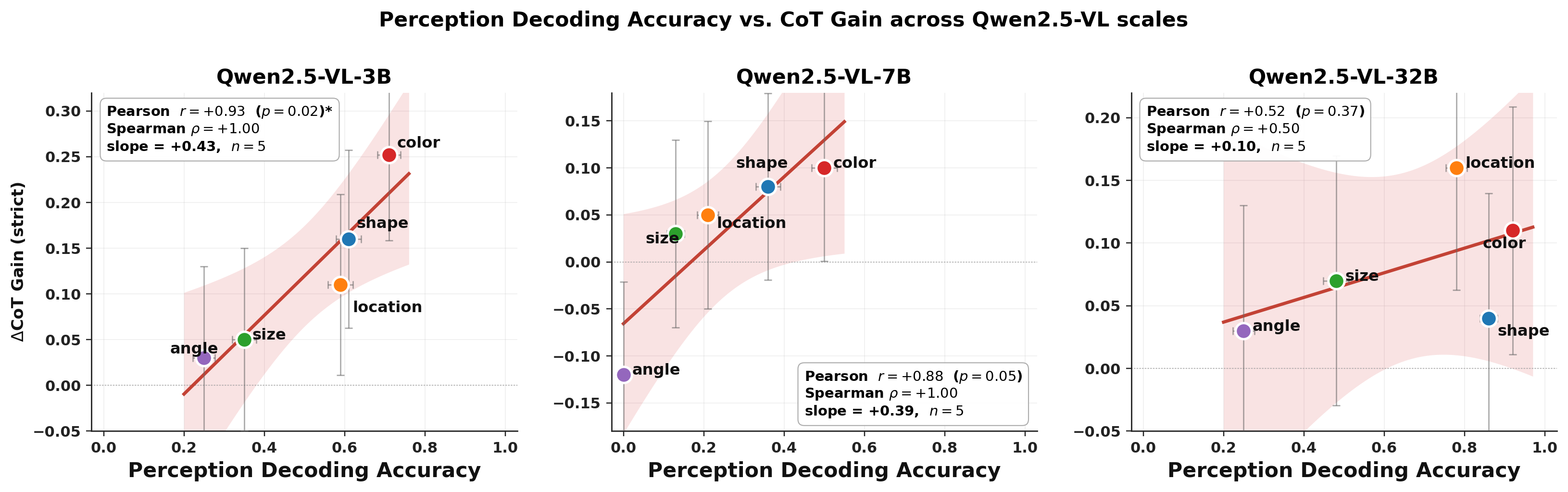
The relationship is positive at every scale. Attributes with relatively higher readout accuracy within each scale tend to show larger CoT gains, whereas attributes with weaker readout (angle and size at every scale) show essentially no CoT gain or slightly negative gain. At 32B, three of five attributes saturate above readout accuracy \(0.77\), compressing residual variance. We therefore read \(\rho\) as the more stable summary at high scale and the linear coefficient as a within-readout-range slope. The angle limiting case (chance-level readout, VAB ill-defined) is in Appendix 10.7.
Because the reasoning operation is held fixed across attributes, the variation in CoT gain is difficult to explain by reasoning difficulty alone. CoT improves counting only after the queried visual attribute is available as a usable symbol, complementing Section 5 by identifying what limits CoT once extended visual access is not the source of improvement.
6.3 Symbolic-attribute oracle bypass↩︎
The correlation in Figure 5 is observational. Hard attributes may show small CoT gains either because the model cannot read out the relevant visual attribute, or because the corresponding counting question is intrinsically difficult to solve. To separate these possibilities, we run an oracle-bypass experiment.
In this setting, we use the same Qwen2.5-VL-3B checkpoint without image tokens. No image is provided, the visual-token pathway is bypassed, and ground-truth object attributes are serialized directly into the prompt. The model is then asked the same multiple-choice counting questions under Direct and CoT prompting. The experiment therefore does not test visual perception. It tests whether the language-side counting operation can benefit from CoT once the relevant attributes are already available as symbols.
We consider two oracle inputs. The minimal oracle provides only the queried attribute for each object (e.g., color values when the question asks about color counting). This is the cleanest test because it removes the visual readout step while preserving the counting operation. The full oracle provides all object attributes, adding irrelevant information and serving as a robustness condition rather than the primary evidence.
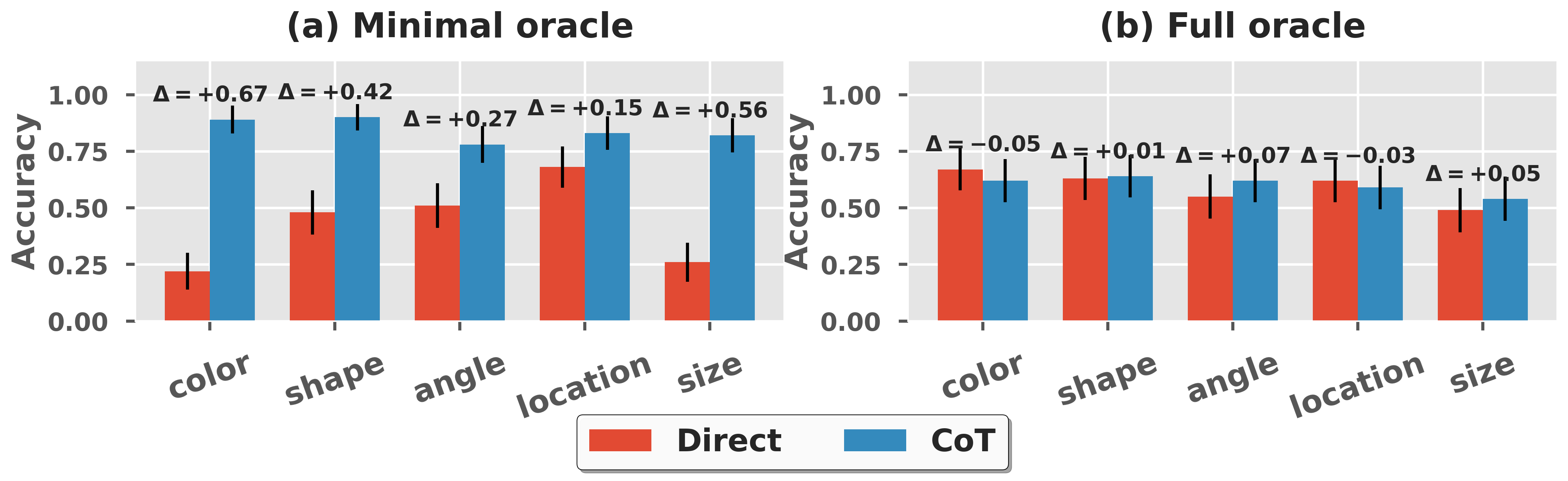
Figure 6 (a) shows that under the minimal oracle, CoT gains become consistent across attributes, including angle, size, and location, which showed weak gains under image input (Figure 5). The counting operation is therefore not the limiting factor once the relevant attributes are supplied as symbols. The limiting step is making the queried visual attribute available in a usable symbolic form. Figure 6 (b) reports the full-oracle condition, where the larger prompt changes the amount of irrelevant information and the headroom for CoT gains. We treat it as a supplementary check.
The probe-decode gap and the oracle bypass together separate three quantities that are easy to conflate. Linear probing asks whether the attribute is present in hidden states (Section 6.1). Direct decoding asks whether the model can read out the attribute as a usable symbol (Section 6.2). Oracle bypass asks whether the counting operation can benefit from CoT once that symbol is supplied (this section). The results point to the middle step as the bottleneck. CoT can improve reasoning over available symbols, but it does not reliably recover a visual attribute that the model cannot itself read out.
7 Discussion↩︎
7.0.0.1 Interpreting the VAB.
This work provides a causal test of what is extended when VLMs generate longer CoT traces. Across the regimes tested here, Visual Access Sweep reveals a finite Visual Access Boundary under both Direct and CoT prompting. Extended generation does not require continued direct image-token access throughout the reasoning trace. Operationally, the VAB marks when additional direct attention from generated-token queries to image-token keys becomes functionally unnecessary. It does not imply that visual evidence is absent from the model. Such evidence may already have been transformed into hidden-state representations and carried forward through the residual stream. This reframes visual-attention decay and visual forgetting. The key question is not whether attention to image tokens decreases, but whether later direct access is still necessary for the task.
7.0.0.2 Implications for CoT and active perception.
The perceptual-readout results suggest that CoT helps when the needed visual attribute has first been made available in a form the model’s reasoning trace can use. When readout succeeds, longer reasoning can improve the downstream counting operation. When readout fails, CoT does not reliably recover the missing symbol, even if latent visual information may be present. This gives a practical rule for test-time scaling: before spending tokens on longer reasoning, test whether the relevant visual attribute can be read out reliably. Within Qwen2.5-VL, a cheap multi-object readout probe supports such routing, preserving most of the always-CoT accuracy at substantially lower token cost (Appendix [app:routing]). The same result clarifies the role of active perception methods such as MemVR [19], Look-Back [20], and Visual Perception Token [21]. These methods are complementary: ordinary CoT in the tested regime does not by itself close the perception-reasoning loop, whereas active perception methods explicitly try to acquire new visual evidence conditioned on the reasoning state.
7.0.0.3 Scope and limitations.
The evidence in this paper covers controlled attribute-counting tasks across families and scales, a GQA-derived real-image setting, and an additional cross-attention fusion setting (Appendix 10.5). Tasks deliberately designed to require iterative visual inspection remain outside the current evaluation. The sweep result also does not by itself identify the internal mechanism that produces the boundary. The same VAB pattern could arise because visual attributes are bound into hidden-state representations early, because late layers receive sufficient image-derived information through the residual stream, or because CoT prompting front-loads visual extraction into early generated tokens. Visual Access Sweep isolates the necessity of one channel (direct generated-token-to-image-token attention), so distinguishing these accounts will require complementary interventions on the residual stream and on the temporal distribution of perceptual extraction.
We thank our colleagues for their valuable discussions and feedback throughout the development of this work.
8 Experimental Details↩︎
8.1 Dataset Generation↩︎
We construct controlled synthetic tasks in which the queried visual attribute varies while the counting operation is held fixed. Images are 256\(\times\)256 px RGB generated with matplotlib under a fixed
random seed. Tables 1 and 2 summarize the controlled attributes and dataset sizes.
| Attribute | Classes |
|---|---|
| Color | red / green / yellow / blue |
| Shape | star / circle / triangle / square |
| Size | xs (18 px) / s (24 px) / l (30 px) / xl (36 px) |
| Location | four image quadrants |
| Angle | 0\(^\circ\) / 45\(^\circ\) / 90\(^\circ\) / 135\(^\circ\) |
| Task | Images | Objects | Queries |
|---|---|---|---|
| Single-object readout | 750 | 1 | one attribute query per image |
| Counting | 150 | 6–7 | five queries per image |
8.2 Task Examples↩︎
Figure 7 shows one multi-object counting instance with its per-object attributes and the five corresponding queries.
8.3 Prompting, decoding, and answer extraction↩︎
We use a unified prompt template across all models with greedy decoding on frozen public checkpoints. Table 3 summarizes the prompt instructions and answer-extraction rules across settings, and Table 4 lists the verbatim prompt strings. For Direct, CoT, and Oracle counting, option keys are randomly permuted per query and extracted from the model output (no constrained decoding). GQA dataset construction details are in Appendix 10.6.
| Setting | Prompt instruction | Answer extraction |
|---|---|---|
| Direct counting | answer with option key only | option-key extraction (A–E) |
| CoT counting | think step by step, then answer in braces | final braced option key (A–E) |
| Single-object readout | multiple-choice attribute question (Table [tbl:tab:app95prompts95verbatim]) | option-key extraction (A–E) |
| Multi-object readout | fill missing target attribute per object, JSON output (Table [tbl:tab:app95prompts95verbatim]) | per-object value parse from JSON |
| GQA Direct | short-answer format with curly-brace final line | last “yes” / “no” (yn_last) |
| GQA CoT | think step by step, finish with curly-brace final line | last “yes” / “no” (yn_last) |
| Oracle (counting) | serialized attributes as text (minimal or full) | option-key extraction (A–E) |
| Setting | Prompt body |
|---|---|
| Counting / Direct | How many {attribute_value} objects are in the image? options: {A: 2, B: 4, C: 1, D: 3, E: 5} Answer with the option key only (no ’:’ or value). Respond with a single final line in the curly braces format: {A} |
| Counting / CoT | How many {attribute_value} objects are in the image? options: {A: 2, B: 4, C: 1, D: 3, E: 5} Think step by step. You must write intermediate steps. Respond in curly braces format: {A} |
| Single-object readout | Which color is this object in the image? options: {A: blue, B: red, C: green, D: yellow} Answer with the option key only (no ’:’ or value). Respond with a single final line in the curly braces format: {A} |
| Multi-object readout | In the image, there are {N} objects. Fill in the missing color for each object. Valid color values: red, green, yellow, blue Object 0: color=__, shape=triangle, size=l, location=upper_left, angle=135 Object 1: color=__, shape=circle, size=s, location=lower_right, angle=0 … Output in following format: {"objects": [{"id": 0, "color": "red"}, {"id": 1, "color": "green"}, …]} |
| GQA / Direct | {question} Answer with a short phrase only. Respond with a single final line in the curly braces format: Answer: {your short answer} |
| GQA / CoT | {question} Think step by step. You must write intermediate steps. Finish with a single final line in the curly braces format after your reasoning: Answer: {your short answer} |
| Oracle (minimal) | In the image, there are {N} objects. Object 0: color=blue Object 1: color=yellow … How many {attribute_value} objects are there in the image? Answer with the option key only (no ’:’ or value). Respond with a single final line in the curly braces format: {A} |
| Oracle (full) | In the image, there are {N} objects. Object 0: color=blue, shape=star, size=l, location=lower_right, angle=0 Object 1: color=yellow, shape=circle, size=s, location=upper_left, angle=135 … How many {attribute_value} objects are there in the image? Answer with the option key only (no ’:’ or value). Respond with a single final line in the curly braces format: {A} |
8.4 Compute Resources↩︎
All experiments in this paper are inference-time interventions on frozen public VLM checkpoints. No VLM is fine-tuned. Only lightweight linear probes are trained for the probe-vs-decode analysis (Appendix 11.1). Hardware and runtime are summarized in Table 5. Aggregate compute across the main results reported in this paper is on the order of \(\sim 1{,}100\) GPU-hours, and preliminary or discarded experiments (alternative sweep grids, additional probe configurations, control runs not reported) account for a comparable additional amount.
| Experiment family | Hardware | Approx. runtime |
|---|---|---|
| (Qwen2.5-VL-3B/7B, InternVL3-8B, Llama-3.2-11B-Vision) | \(3\times\) H100 NVL 96 GB | \(\sim 600\) GPU-hours |
| (Qwen2.5-VL-32B, InternVL3-14B/38B) | \(3\times\) H100 NVL 96 GB | \(\sim 500\) GPU-hours |
| Qwen2.5-VL-32B 2D layer-\(\times\)-token sweep | \(3\times\) H100 NVL 96 GB | 45–60 GPU-hours |
| (probe, oracle, controls) | \(3\times\) H100 NVL 96 GB | \(\sim 21\) GPU-hours |
| Total reported main results | — | \(\sim 1{,}100\) GPU-hours |
Peak GPU memory is bounded by full-attention forward-pass memory at the largest scale (Qwen2.5-VL-32B) with the image-token prefix, and fits within \(3\times\) H100 NVL 96 GB with standard tensor-parallel sharding.
9 Visual Access Sweep: Methodology Details↩︎
This section reports two intervention controls and an \(\epsilon\)-sensitivity analysis for Visual Access Sweep.
9.1 Control Experiments: Ruling Out Intervention Artifacts↩︎
We run two controls targeting possible artifacts of Visual Access Sweep.
9.1.0.1 Late-layer query-text block.
The first concern is a query-mediated re-reading loophole. Even if generated tokens cannot directly attend to image tokens in late layers, prompt or query-text tokens might still attend to the image in those layers and pass image-derived information to generated tokens. To test this, we apply a stricter intervention that additionally blocks query-text \(\to\) image-token attention from the same cutoff layer upward. Importantly, early-layer query-text access is left unchanged. The control only removes the late-layer path that could bypass the generated-token intervention. Figure 8 shows that the qualitative VAB pattern is preserved under this stricter intervention.


Figure 8: Late-layer query-text block control (Color Counting, Qwen2.5-VL-32B). In addition to blocking generated-token \(\to\) image-token attention, this control blocks query-text \(\to\) image-token attention from the same cutoff layer upward. Early-layer query-text access is left intact. The qualitative VAB pattern is preserved, weakening the query-mediated late-rereading explanation.. a — Direct layer sweep., b — CoT layer-token sweep.
9.1.0.2 Null-sink control.
The second concern is an attention-redistribution artifact. Setting image-token logits to \(-\infty\) changes the softmax normalization over the remaining real tokens, which could in principle distort the model’s behavior beyond simply removing image access. To test whether the observed boundary is caused by this redistribution rather than by removing image access, we redirect the removed image-token attention mass to a dummy non-visual sink slot. Figure 9 shows that the qualitative VAB pattern is again preserved.


Figure 9: Null-sink control (Color Counting, Qwen2.5-VL-32B). Removed image-token attention mass is redirected to a dummy non-visual sink instead of being redistributed over real non-image tokens. The qualitative VAB pattern is preserved, weakening the attention-redistribution artifact explanation.. a — Direct layer sweep., b — CoT layer-token sweep.
9.1.0.3 Takeaway.
Together, these controls support the interpretation that the reported boundary is not primarily caused by either query-mediated late re-reading or attention-mass redistribution. They do not claim that all visual information flow stops after the boundary. Rather, they support the narrower claim used throughout the paper. Additional late direct image-token access is not functionally necessary in the tested setting.
9.2 VAB Sensitivity to the Tolerance Parameter \(\epsilon\)↩︎
The VAB definition (Section 4.2) depends on a tolerance \(\epsilon\), which we fix to \(\epsilon = 0.05\) throughout the main text. A natural concern is that the CoT-vs-Direct boundary comparison in Section 5.2 could rest on this specific choice of \(\epsilon\). To check this, we recompute \(\ell^*\) on Qwen2.5-VL-32B for color and shape counting under both criteria across \(\epsilon \in \{0.03, 0.05, 0.07, 0.10\}\) (Table ¿tbl:tab:eps95sensitivity?).
l l r >cr r r r >cr r r & & &
(lr)3-6 (lr)7-10 Task & & \(\epsilon{=}0.03\) & \(\epsilon{=}0.05\) & \(\epsilon{=}0.07\) & \(\epsilon{=}0.10\) & \(\epsilon{=}0.03\) & \(\epsilon{=}0.05\) & \(\epsilon{=}0.07\) & \(\epsilon{=}0.10\)
& \(\ell^*_{\mathrm{D}}\) & 44 & 43 & 43 & 42 & 44 & 43 & 43 & 42
& \(\ell^*_{\mathrm{DA}}\) / \(\ell^*_{\mathrm{CoT}}\) & 43 & 43 & 42 & 42 & 52 & 52 & 52 & 51
& \(\Delta\ell^*_{\mathrm{DA}}\) & \(-1\) & \(\boldsymbol{0}\) & \(-1\) & \(0\) & — & — & — & —
& \(\Delta\ell^*_{\mathrm{own}}\) & — & — & — & — & \(+8\) & \(\boldsymbol{+9}\) & \(+9\)
& \(+9\)
& \(\ell^*_{\mathrm{D}}\) & 42 & 42 & 42 & 42 & 42 & 42 & 42 & 42
& \(\ell^*_{\mathrm{DA}}\) / \(\ell^*_{\mathrm{CoT}}\) & 42 & 42 & 42 & 41 & 44 & 43 & 43 & 42
& \(\Delta\ell^*_{\mathrm{DA}}\) & \(0\) & \(\boldsymbol{0}\) & \(0\) & \(-1\) & — & — & — & —
& \(\Delta\ell^*_{\mathrm{own}}\) & — & — & — & — & \(+2\) & \(\boldsymbol{+1}\) & \(+1\)
& \(0\)
9.2.0.1 Takeaway.
Two points are stable across tolerance choices. First, under the direct-anchored criterion, the CoT boundary remains close to the Direct boundary across all tested \(\epsilon\) values (\(|\Delta\ell^*_{\mathrm{DA}}| \le 1\)), so the main CoT-Direct comparison is not an artifact of choosing \(\epsilon = 0.05\). Second, under the CoT-own-max criterion the boundary can be deeper because the target accuracy is higher. This reflects the stricter accuracy target rather than a proportional expansion of direct image-token access with generation length.
10 Visual Access Boundary: Detailed Results↩︎
This section reports per-family, per-scale, and per-task VAB results supporting Section 5: boundary summary tables, model architectures compared, family-level sweeps for Qwen2.5-VL and InternVL3, a cross-attention fusion pilot, the GQA real-image extension, an angle-attribute limiting case, and a qualitative error breakdown.
10.1 Boundary Summary Tables↩︎
Tables 6 and 7 report the per-setting VAB layers used in Section 5. The CoT-own-max criterion asks when CoT preserves its own full-access accuracy, whereas the direct-anchored criterion asks when CoT reaches Direct’s full-access accuracy. We denote the corresponding CoT-side boundaries by \(\ell^*_{\mathrm{CoT}}\) and \(\ell^*_{\mathrm{DA}}\), respectively, and report shifts relative to the Direct boundary \(\ell^*_{\mathrm{D}}\) following Eq. (2 ). We report both criteria because they answer different questions. The former measures the access region needed for CoT’s own ceiling, while the latter controls for Direct–CoT ceiling differences. N/A in Table 7 indicates that CoT never reaches the direct-anchored target in that setting, so the boundary is undefined under this criterion.
| Color Counting | Shape Counting | ||||||||
| Model | \(\boldsymbol{L}\) | \(\boldsymbol{\ell^*_{\mathrm{D}}}\) | \(\boldsymbol{\ell^*_{\mathrm{CoT}}}\) | \(\boldsymbol{\Delta\ell^*_{\mathrm{own}}}\) | \(\mathbb{E}[\boldsymbol{T_{\text{gen}}}]\) | \(\boldsymbol{\ell^*_{\mathrm{D}}}\) | \(\boldsymbol{\ell^*_{\mathrm{CoT}}}\) | \(\boldsymbol{\Delta\ell^*_{\mathrm{own}}}\) | \(\mathbb{E}[\boldsymbol{T_{\text{gen}}}]\) |
| Qwen2.5-VL-3B | 36 | 25 | 34 | \(+9\) | \(128 \pm 32\) | 22 | 29 | \(+7\) | \(142 \pm 29\) |
| Qwen2.5-VL-7B | 28 | 20 | 21 | \(+1\) | \(85 \pm 33\) | 20 | 19 | \(-1\) | \(76 \pm 18\) |
| Qwen2.5-VL-32B | 64 | 43 | 52 | \(+9\) | \(183 \pm 33\) | 42 | 44 | \(+2\) | \(143 \pm 30\) |
| InternVL3-8B | 28 | 20 | 26 | \(+6\) | \(105 \pm 20\) | 20 | 23 | \(+3\) | \(103 \pm 27\) |
| InternVL3-14B | 48 | 36 | 36 | \(0\) | \(75 \pm 17\) | 35 | 37 | \(+2\) | \(86 \pm 17\) |
| InternVL3-38B | 64 | 45 | 44 | \(-1\) | \(66 \pm 11\) | 46 | 47 | \(+1\) | \(92 \pm 21\) |
| Color Counting | Shape Counting | ||||||
| Model | \(\boldsymbol{L}\) | \(\boldsymbol{\ell^*_{\mathrm{D}}}\) | \(\boldsymbol{\ell^*_{\mathrm{DA}}}\) | \(\boldsymbol{\Delta\ell^*_{\mathrm{DA}}}\) | \(\boldsymbol{\ell^*_{\mathrm{D}}}\) | \(\boldsymbol{\ell^*_{\mathrm{DA}}}\) | \(\boldsymbol{\Delta\ell^*_{\mathrm{DA}}}\) |
| Qwen2.5-VL-3B | 36 | 25 | 33 | \(+8\) | 22 | N/A | N/A |
| Qwen2.5-VL-7B | 28 | 20 | 20 | \(0\) | 20 | 5 | \(-15\) |
| Qwen2.5-VL-32B | 64 | 43 | 43 | \(0\) | 42 | 42 | \(0\) |
| InternVL3-8B | 28 | 20 | N/A | N/A | 20 | N/A | N/A |
| InternVL3-14B | 48 | 36 | 34 | \(-2\) | 35 | 37 | \(+2\) |
| InternVL3-38B | 64 | 45 | 46 | \(+1\) | 46 | 47 | \(+1\) |
10.2 Model Architectures Compared↩︎
Table 8 summarizes the architectural differences across the VLMs analyzed in this paper. The cross-attention fusion VLM (Llama-3.2-11B-Vision-Instruct2) is reported in Appendix 10.5.
| Family | Scale | Decoder layers | Vision encoder / connector | Fusion |
|---|---|---|---|---|
| [36] | 3B / 7B / 32B | 36 / 28 / 64 | Qwen ViT + MLP | Prefix |
| [37] | 8B / 14B / 38B | 28 / 48 / 64 | InternViT + MLP | Prefix |
| [38] | 11B | 40 | CLIP ViT + cross-attn | Cross-attention |
10.3 Qwen2.5-VL Family Sweeps↩︎
Figure 10 shows per-scale Direct VAB curves and CoT VAB heatmaps for the Qwen2.5-VL family.
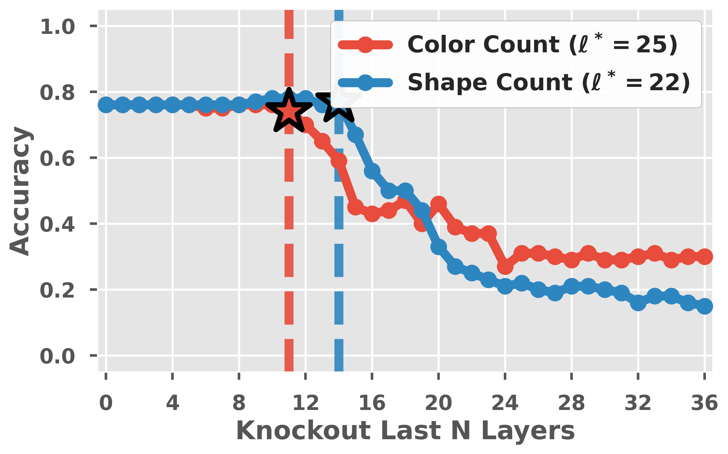


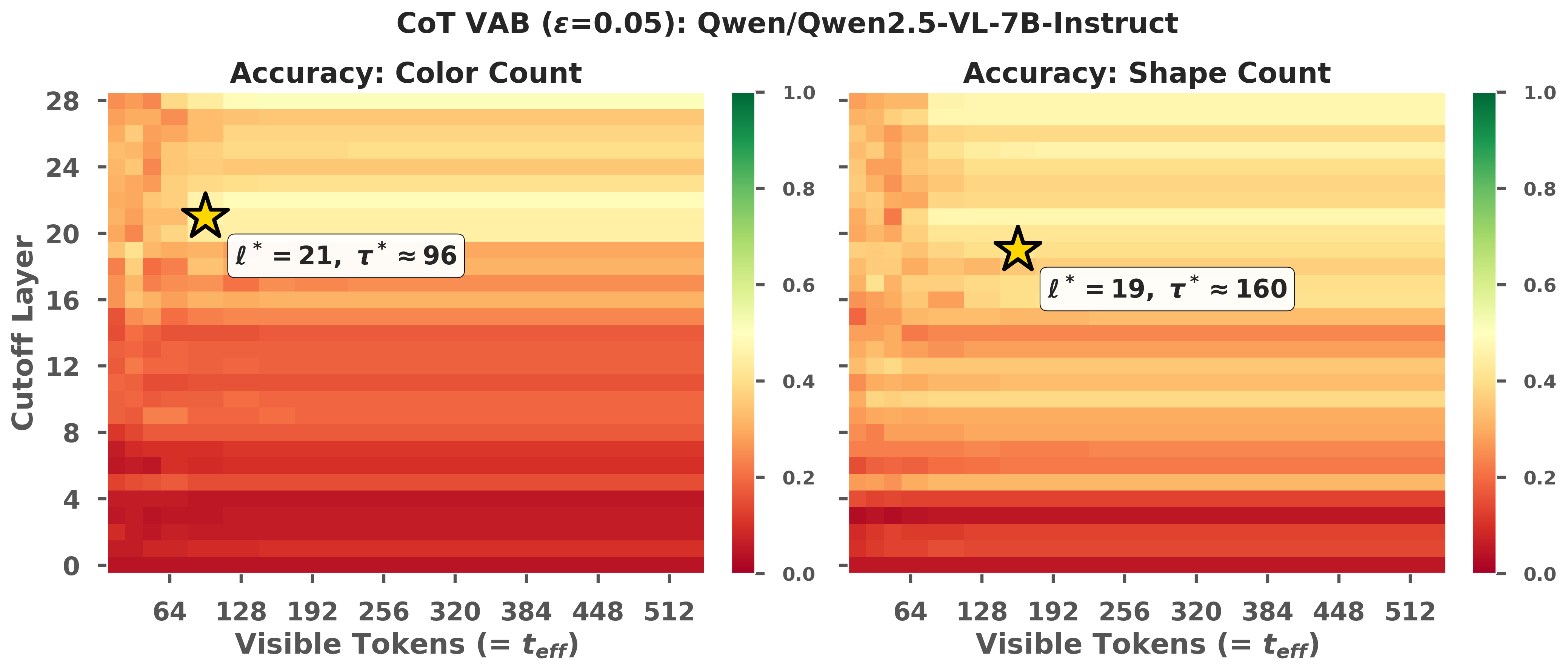
Figure 10: Qwen2.5-VL family sweeps. Rows correspond to model scale; left panels show Direct layer sweeps and right panels show CoT layer-token sweeps. Exact boundary values are reported in Tables 6 and 7.. a — 3B Direct., b — 3B CoT., c — 7B Direct., d — 7B CoT., e — 32B Direct., f — 32B CoT.
10.4 InternVL3 Family Sweeps↩︎
To assess whether the VAB phenomenon generalizes across model families, we additionally evaluated InternVL3 models (8B, 14B, 38B). These models use a different vision encoder and projection architecture compared to Qwen2.5-VL.
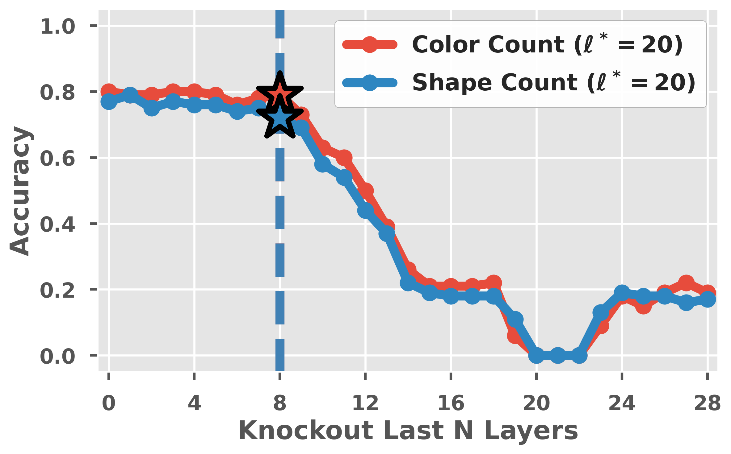
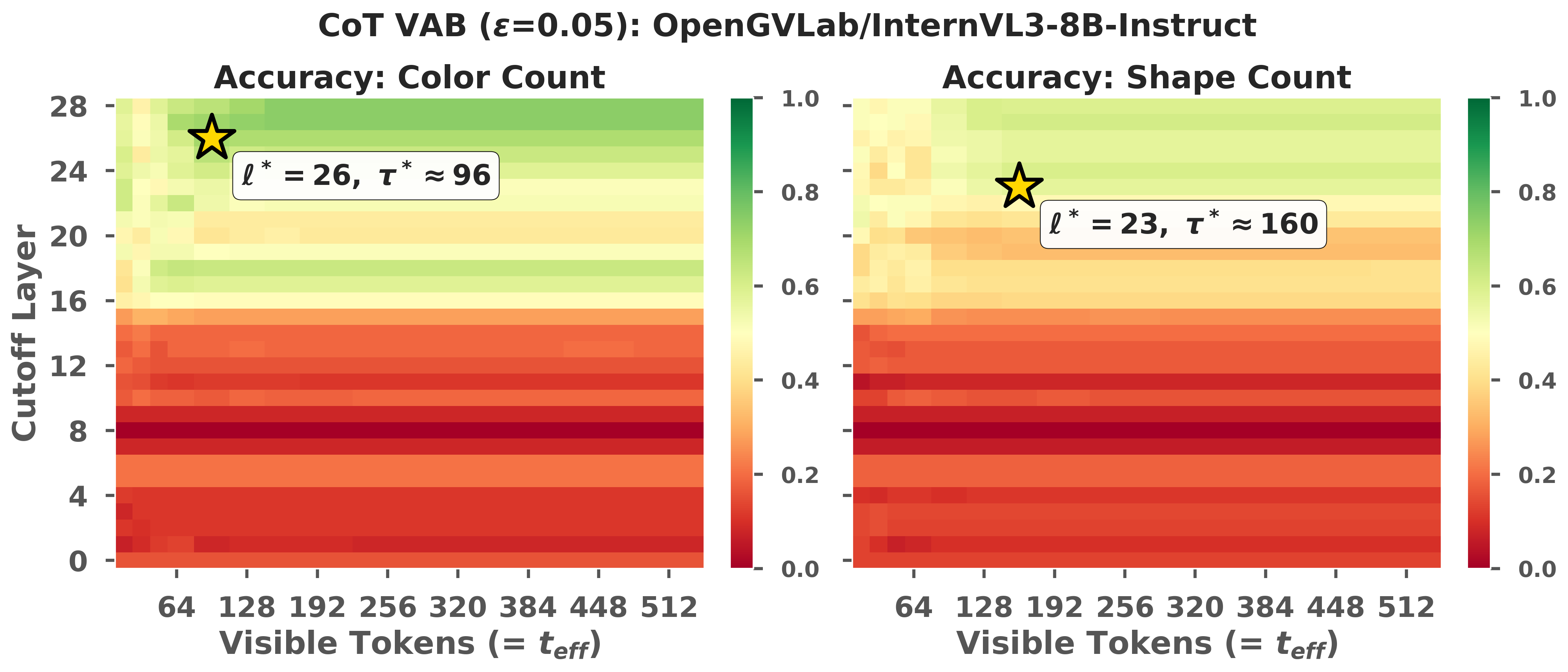
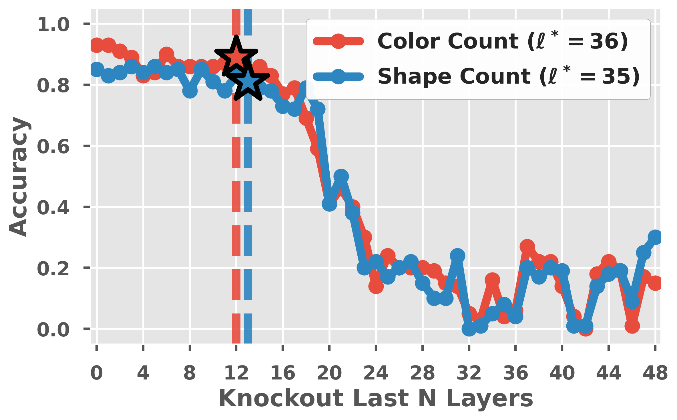
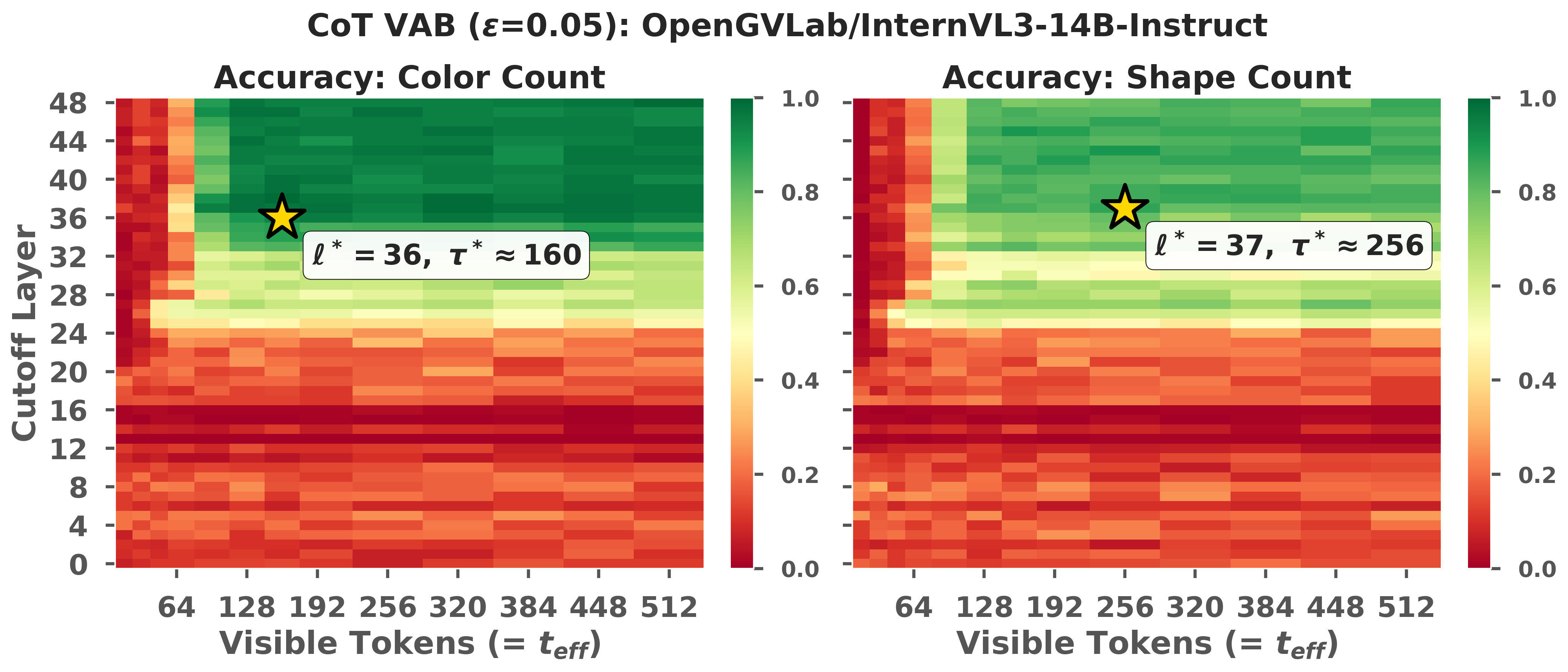
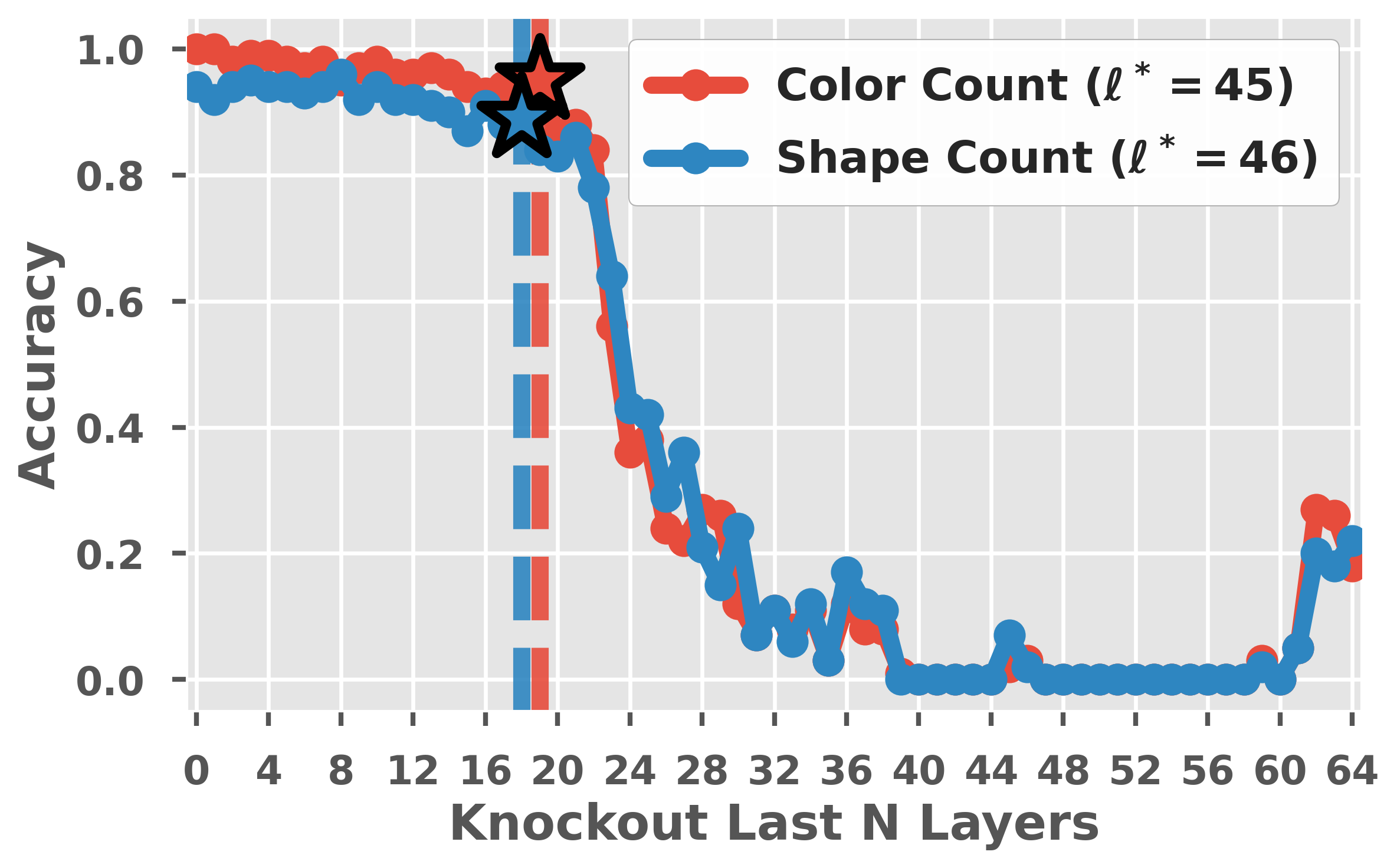
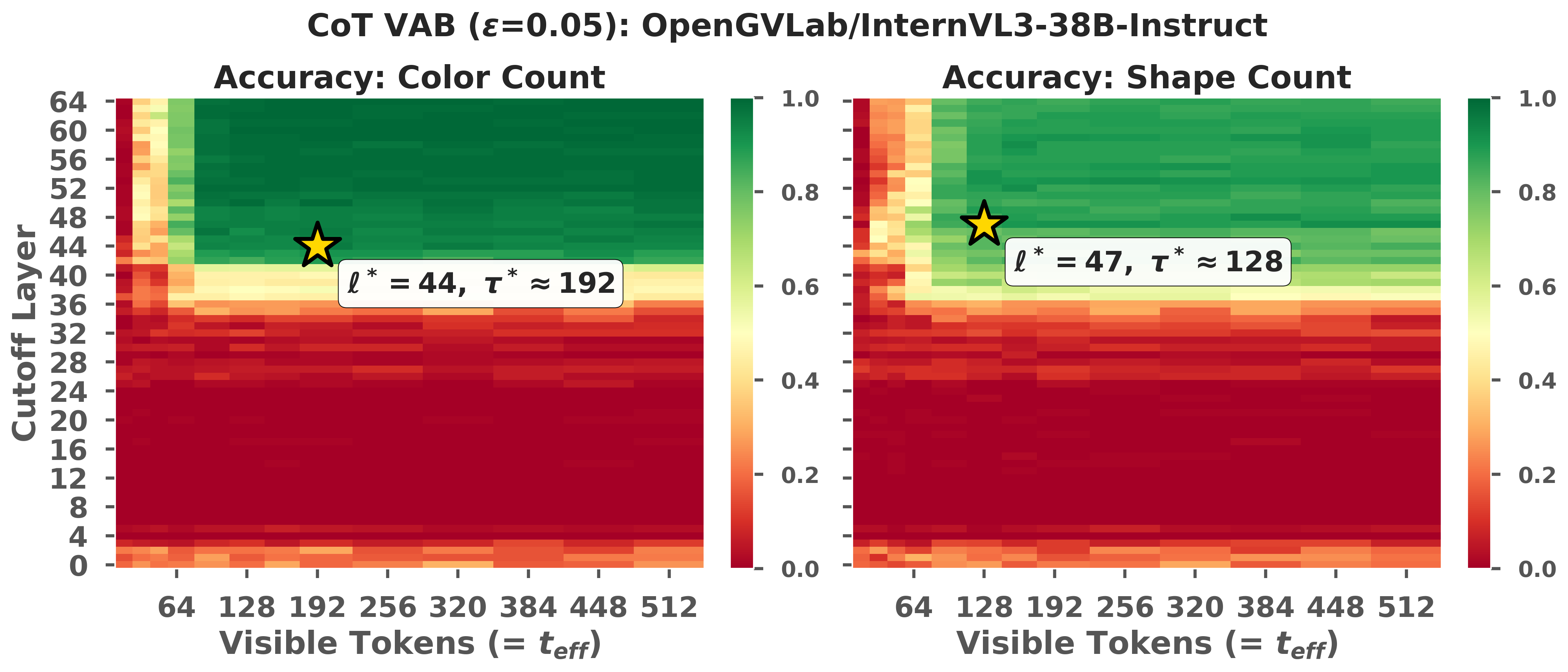
Figure 11: InternVL3 family sweeps. Rows correspond to model scale; left panels show Direct layer sweeps and right panels show CoT layer-token sweeps. Exact boundary values are reported in Tables 6 and 7.. a — 8B Direct., b — 8B CoT., c — 14B Direct., d — 14B CoT., e — 38B Direct., f — 38B CoT.
10.5 Cross-Attention Fusion Pilot↩︎
The main experiments use prefix-fusion VLMs, where image tokens are concatenated with text tokens and direct visual access is realized through self-attention from generated-token queries to image-token keys. As a pilot check, we apply the same intervention principle to Llama-3.2-11B-Vision-Instruct, where visual features are exposed through cross-attention modules rather than through an image-token prefix. In this case, the sweep masks generated-token queries’ cross-attention to visual keys over layer depth and generation time.
We report the CoT-side sweep only. Direct prompting on this model did not reliably follow the option-key answer format under our extraction protocol, so the Direct layer sweep was not a clean comparison. This result should therefore be read as an intervention-transfer check for cross-attention fusion, not as a full family-level comparison.

10.6 GQA Real-Image Extension↩︎
Table 9 summarizes the construction and evaluation protocol for the GQA yes/no extension. This experiment is used as a real-image check of the VAB structure, not as a claim that CoT improves GQA accuracy. We
extract the final occurrence of \b(yes|no)\b (case-insensitive) as the predicted label.
| Item | Value |
|---|---|
| Source split | val_balanced |
| Filter | answer \(\in\) (case-insensitive) |
| Sample size | 100, shuffled with seed \(0\) |
| Label balance | 53 no / 47 yes (chance level \(0.5\)) |
| Model | Qwen2.5-VL-32B |
| Image preprocessing | RGB conversion, resize to model native input |
| Extraction rule | last yes/no token (yn_last) |
| Direct full accuracy / \(\ell^*\) | \(0.84\) / \(40\) (\(N^* = 24\)) |
| CoT full accuracy / \((\ell^*, \tau^*)\) | \(0.80\) / \((28,\, \approx\!32)\) |
A finite VAB appears in both Direct and CoT sweeps, even though CoT does not improve over Direct on this binary-answer subset. This supports the main-text claim that the VAB phenomenon extends beyond synthetic stimuli (Section 5.4), independent of whether CoT itself improves task accuracy.
10.7 Limiting Case: Angle Counting↩︎
Figure 13 shows angle counting on Qwen2.5-VL-32B. We include this as a limiting case rather than as main VAB evidence. When full-access accuracy is near the task floor, the sweep cannot cleanly localize a boundary, because preserving low accuracy is not informative about successful visual grounding. This case supports the interpretation used in Section 6: extended reasoning cannot compensate when the queried visual attribute is not reliably read out into a usable symbol.
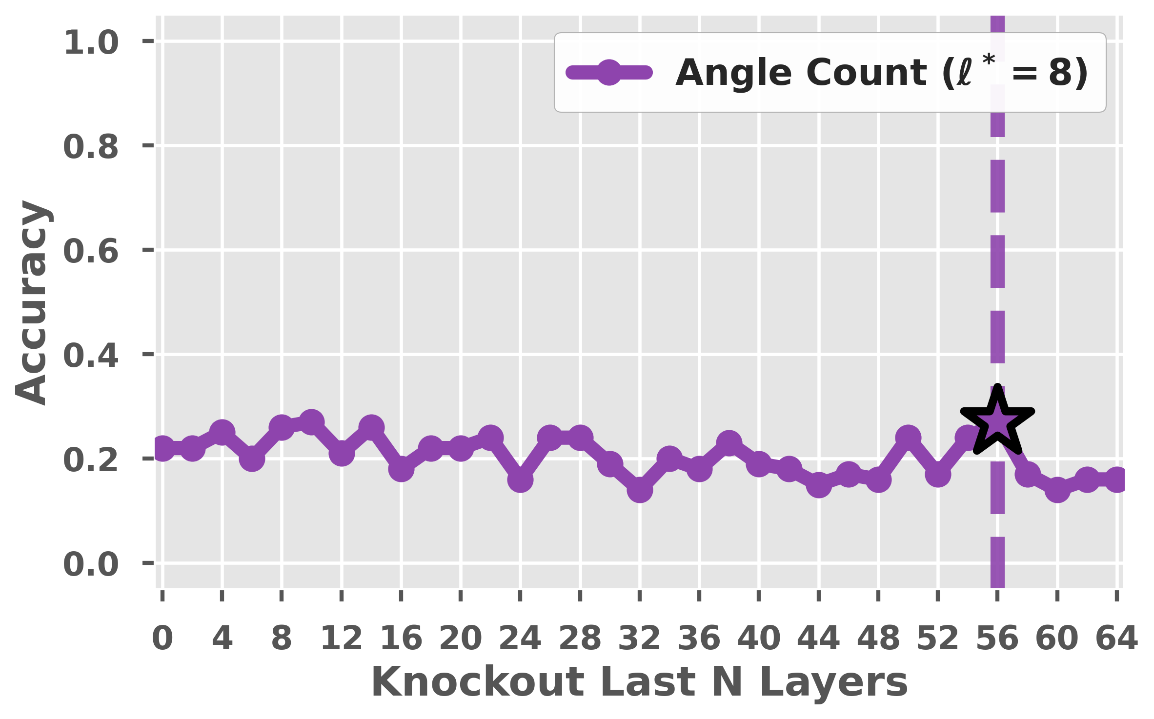

Figure 13: Angle counting as a limiting case (Qwen2.5-VL-32B). Full-access performance is near the task floor, so the sweep does not yield an interpretable boundary in the same sense as color or shape counting.. a — Direct layer sweep., b — CoT layer-token sweep.
10.8 Qualitative Error Breakdown↩︎
Table 10 provides a small qualitative breakdown of representative errors. We use it only to characterize failure modes, not as a main quantitative result. Errors are grouped into four categories: alt-attribute-consistent, where the predicted count matches the count of a non-target attribute value in the same scene; tally-inconsistent, where the target attribute is identified but the written count disagrees with the visible tally; format errors, where outputs fail extraction (no valid option key or yes/no token); and other errors that match none of the above.
10.8.0.1 Takeaway.
When direct visual access is blocked before the VAB, errors are mostly alt-attribute-consistent, suggesting that the intervention corrupts which visual attribute or value is available for counting. Under full-access CoT, the remaining errors shift toward tally inconsistency, suggesting that once the visual attribute is available, residual failures more often occur in the symbolic counting step.
| Task | Condition | Acc | Alt-attr.cons. | Tally incon. | Other | Format |
|---|---|---|---|---|---|---|
| color | Full access (Direct) | 0.80 | 20 | 0 | 0 | 0 |
| color | Beyond VAB (\(\ell{=}36\)) | 0.35 | 65 | 0 | 0 | 0 |
| color | Strong block (\(\ell{=}16\)) | 0.35 | 65 | 0 | 0 | 0 |
| color | CoT full access | 0.95 | 0 | 4 | 1 | 0 |
| shape | Full access (Direct) | 0.84 | 16 | 0 | 0 | 0 |
| shape | Beyond VAB (\(\ell{=}34\)) | 0.49 | 51 | 0 | 0 | 0 |
| shape | Strong block (\(\ell{=}16\)) | 0.20 | 80 | 0 | 0 | 0 |
| shape | CoT full access | 0.89 | 0 | 9 | 2 | 0 |
| angle | Full access (Direct) | 0.22 | 77 | 0 | 0 | 1 |
| angle | CoT full access | 0.37 | 0 | 61 | 0 | 2 |
11 Perceptual Readout: Detailed Results↩︎
This section reports two pieces of supporting evidence for Section 6: a probe-vs-decode comparison that separates latent visual grounding from decoded readout, and a per-attribute breakdown of the readout–CoT-gain relationship underlying Figure 5.
11.1 Probe-vs-Decode Gap↩︎
This appendix uses a single-object setting only for the probe-vs-decode diagnostic. This is separate from the multi-object perceptual readout accuracy used as the Figure 5 predictor in Section 6. The goal here is to test whether attribute information is present in hidden states even when the model’s own decoded answer is unreliable. Table ¿tbl:tab:s1-probing-decoding? reports this comparison on Qwen2.5-VL-32B. An attribute can be linearly recoverable from hidden states (Probing Acc) while still being unavailable to the model as a decoded output symbol (Decoding Acc).
@l c c >cc@ Attribute & Probing Acc & Decoding Acc & Gap (Probe \(-\) Decode)
Color & 1.000 & 1.000 & 0.000
Shape & 1.000 & 1.000 & 0.000
Angle & 0.954 & 0.383 & \(+\)0.571
Location & 0.971 & 0.312 & \(+\)0.658
Size & 0.892 & 0.283 & \(+\)0.608
| Item | Value |
|---|---|
| Model | Qwen2.5-VL-32B |
| Layer | Final decoder layer (after the last Transformer block) |
| Token position | Final image-token position |
| Data | 500 single-object images, 400 / 100 train-validation split |
| Probe | \(\ell_2\)-regularized multinomial logistic regression (\(\lambda = 1.0\), scikit-learn) |
| Evaluation | Held-out accuracy on the 100-image validation split |
11.2 Per-Attribute CoT Gain↩︎
Table ¿tbl:tab:app95cross95scale95corr? reports the per-attribute values underlying Figure 5. Each block corresponds to one Qwen2.5-VL scale. Within each block, attributes are ordered by multi-object perceptual readout accuracy. Pearson \(r\) and Spearman \(\rho\) are descriptive summaries over five attributes per scale, not independent evidence of a universal scaling law.
11.2.0.1 Takeaway.
Across Qwen2.5-VL scales, attributes with stronger multi-object readout generally show larger CoT gains, while attributes with weak readout show small or negative gains. Together with the oracle result in Figure 6, this supports the interpretation in Section 6: CoT gain is constrained by whether the queried visual attribute is available as a usable symbol.
@l c c c r@ Attribute & Readout & Direct & CoT & \(\boldsymbol{\Delta}\)CoT
color & 0.713 & 0.580 & 0.830 & \(+\)0.250
shape & 0.605 & 0.610 & 0.770 & \(+\)0.160
location & 0.601 & 0.360 & 0.470 & \(+\)0.110
size & 0.347 & 0.140 & 0.190 & \(+\)0.050
angle & 0.245 & 0.290 & 0.320 & \(+\)0.030
color & 0.498 & 0.790 & 0.890 & \(+\)0.100
shape & 0.354 & 0.770 & 0.850 & \(+\)0.080
location & 0.222 & 0.370 & 0.420 & \(+\)0.050
size & 0.131 & 0.310 & 0.340 & \(+\)0.030
angle & 0.005 & 0.440 & 0.320 & \(-\)0.120
color & 0.920 & 0.840 & 0.950 & \(+\)0.110
shape & 0.865 & 0.850 & 0.890 & \(+\)0.040
location & 0.771 & 0.410 & 0.570 & \(+\)0.160
size & 0.479 & 0.200 & 0.270 & \(+\)0.070
angle & 0.254 & 0.370 & 0.400 & \(+\)0.030
12 Practical Implication: Selective CoT Routing↩︎
The perceptual-readout analysis suggests a simple routing heuristic, namely using CoT only when the queried attribute can be reliably read out, and otherwise falling back to Direct inference. For each queried attribute, we route to CoT if the corresponding multi-object readout accuracy on the readout validation split exceeds \(0.5\). This threshold is not tuned for optimal deployment. It is used as a simple illustrative rule. Table 12 shows that this rule preserves most of the accuracy gain of always using CoT while substantially reducing output-token cost.
| Model | Policy | Acc. | Gain vs Direct | Gain recovered | Avg.tokens | Tokens vs CoT |
|---|---|---|---|---|---|---|
| Qwen2.5-VL-3B | Always Direct | 0.396 | — | — | 2.6 | 1.6% |
| Qwen2.5-VL-3B | Always CoT | 0.516 | \(+\)0.120 | 100% | 166.7 | 100% |
| Qwen2.5-VL-3B | Adaptive (thr\(=\)0.5) | 0.500 | \(+\)0.104 | 86.7% | 82.7 | 49.6% |
| Qwen2.5-VL-32B | Always Direct | 0.534 | — | — | 3.0 | 1.3% |
| Qwen2.5-VL-32B | Always CoT | 0.616 | \(+\)0.082 | 100% | 224.3 | 100% |
| Qwen2.5-VL-32B | Adaptive (thr\(=\)0.5) | 0.596 | \(+\)0.062 | 75.6% | 102.9 | 45.9% |
4pt
12.0.0.1 Takeaway.
A cheap attribute-level readout check can recover most of the benefit of always using CoT while avoiding roughly half of the output-token cost in these two representative Qwen2.5-VL settings.