A Mesh-Free Solver for Multi-Phase Mullins–Sekerka Flow: Triple Junctions and Ninety-Degree Boundary Contact
July 14, 2026
Abstract
A bulk mesh-free solver for the multi-phase Mullins–Sekerka flow in \(\mathbb{R}^{2}\) and in a half-plane \(\mathbb{H}\) bounded by a Neumann wall \(\mathcal{W}\) is developed. In the underlying mathematical model, interfaces driven by their curvature are coupled through a harmonic chemical-potential field. We use a charge simulation method, a variant of the method of fundamental solutions: each chemical potential is represented by fundamental solutions centered at charge points off the curve, so no bulk mesh or singular integral is required. It treats curve networks separating several phases at triple junctions, including phases that occupy more than one region; on the half-plane boundary the no-flux condition is imposed exactly by image charges, and mobile contacts stay orthogonal to the wall. The discretization is structure-preserving: between topological events, every bounded phase area is conserved to machine precision at the velocity level by a null-space projection of the discrete area constraints. The junction connectivity is fixed, the only topological event being the disappearance of a region enclosed by a single closed curve and incident to no junction. The proposed scheme is validated against an exact three-concentric-circle solution in terms of convergence, cost, and conditioning.
Key words. multi-phase Mullins–Sekerka flow, charge simulation method, method of fundamental solutions, triple junction, structure-preserving discretization
MSC codes. 65M80, 35R37, 53E10, 80A22
1 Introduction↩︎
When a two-phase mixture is quenched into its miscibility gap, it separates into domains that subsequently coarsen: large domains grow at the expense of small ones, the total interfacial length decreases, and the area of each phase is conserved. In the sharp-interface description of this late-stage Ostwald ripening [1], the phase boundaries move by the Mullins–Sekerka flow [2]. Each interface is driven by its own curvature through a Gibbs–Thomson relation, but the driving force is not local: at every instant one solves for a harmonic bulk field, the chemical potential, whose normal-derivative jump across the interface prescribes the normal velocity. The interfaces communicate only through this bulk field. This non-locality is the source of the flow’s structure: it makes the evolution an \(H^{-1/2}\)-type gradient flow of the interfacial energy that dissipates the total length while preserving the area of each phase [3]. At the same time it is the source of its numerical difficulty, since a global elliptic problem must be solved before the geometry can be advanced by even a single step.
Moving from two phases to many turns the interface into a network of curves meeting at triple junctions, and the evolution of a smooth boundary becomes the evolution of a network with singular vertices. At each junction, the three incident curves obey a force balance, Herring’s angle condition [4], [5] (the symmetric \(120^\circ\) configuration when the surface tensions are equal), together with a balance of diffusive fluxes. The present paper is concerned with the numerical approximation of this multi-phase Mullins–Sekerka flow, both in the whole plane and in a half-plane bounded by a Neumann wall along which interfaces may slide while meeting the wall orthogonally. We keep the junction connectivity of the network fixed; the transitions that alter the junction topology, such as pinch-off and neighbor switching, are outside our scope. We do, however, treat the terminal event of coarsening within a phase: the disappearance of a region enclosed by a single closed interface and incident to no junction, whose area, under the flow, has been transferred to another region of the same phase. The junction structure is thus preserved throughout, while such a single-closed-interface region may vanish once it can no longer be resolved by the mesh. The governing system, together with the notation for the curve–region–phase incidence that a multi-phase configuration requires, is stated precisely in Section 2.
Numerical methods for interfacial flows of this type fall broadly into three families, each with its own strengths and costs. Phase-field methods regularize the sharp interface by a thin diffuse layer and evolve the Cahn–Hilliard equation whose singular limit corresponds to the Mullins–Sekerka flow equation [6]–[9]; they can handle topological changes, but resolving the interfacial layer is expensive, and the junction angle conditions are recovered only asymptotically. Closely related front-capturing schemes like level-set and threshold-dynamics methods [10]–[13] also pass through topological changes while representing the interface implicitly rather than tracking it directly. Boundary integral methods [14]–[18] were the first to discretize the interface alone, representing the harmonic field by a layer potential; they are accurate and dimension-reducing, but the evaluation of singular and nearly-singular integrals is delicate and the extension to several phases and triple junctions is cumbersome; later boundary-integral work has addressed multi-component fluids and Ostwald ripening [19], [20]. Parametric finite element methods [21]–[29] incorporate balance conditions around triple junctions naturally into a variational formulation for various surface evolution equations and have good mesh properties. Moreover, the schemes are unconditionally stable with respect to time steps, and some of these schemes can preserve conservative quantities (e.g., the volume of each phase) at the fully discrete level. However, they still require a mesh of the bulk. Related structure-preserving parametric finite element schemes have also been developed for the multi-phase Mullins–Sekerka problem and a degenerate multi-phase Stefan problem with triple junctions [30]–[32]. None of these families discretizes only the interface, without singular integrals, while also treating triple junctions and boundary contacts.
We pursue a fourth route, based on the charge simulation method (CSM), a variant of the method of fundamental solutions (MFS) [33]–[37]. The idea is to represent each bulk function as a finite combination of fundamental solutions of the Laplacian centered at charge points placed off the interface. Since every basis function is exactly harmonic away from its singular point, the Laplace equation is satisfied automatically, and the only conditions left to enforce are those on the interface itself. No singular integrals arise, since the charge points are held at a positive distance from the collocation points, and no bulk mesh is needed. In this sense, we say that the method is bulk mesh-free and is a boundary-only method, in which the ambient domain has no mesh while the interface is discretized as a polygonal curve. For further details about the MFS, we refer the reader to a review article [38].
A CSM solver for the two-phase Mullins–Sekerka flow, including contact-angle problems on a wall boundary, has been proposed by the author [39]. The contribution of the present paper is to extend that idea to several phases, triple junctions, phases composed of more than one region, and a Neumann boundary. Since the closest existing multi-phase scheme [30] discretizes the problem through a fundamentally different, bulk or whole-domain weak formulation, we do not attempt a direct method-to-method numerical comparison; instead we validate the present method against the exact three-phase solution of [30] (Section 9).
Our discretization is guided by a second principle: structure preservation. For a coarsening flow, approximate area conservation is not sufficient: the phase areas are constant between topological events and change only at such events, and a slow numerical drift would be indistinguishable from physical mass transfer. We therefore treat the discrete area-conservation identities as hard constraints and project the reconstructed velocity onto the corresponding subspace, so that the discrete area fluxes vanish to machine precision (velocity-level conservation, Section 8), independently of the residual of the field solve; the residual drift of the polygonal areas after time stepping is of higher order and is reported in Section 9. Two further ingredients are handled in the same way. The discrete curvature that feeds the Gibbs–Thomson condition is unreliable on the edges adjacent to a triple junction, where a naive evaluation using the junction vertex fails to converge to the interface curvature and biases the reconstructed velocity near the junctions; we correct it locally. And the homogeneous Neumann condition on a straight wall is imposed exactly by reflecting each charge in the wall, at the cost of no additional unknowns.
These ingredients might appear to combine the two-phase charge simulation of [39] with the multi-phase formulation of [30], but the extension is not a simple composition of the two. Collocating the Gibbs–Thomson and continuity conditions on both sides of every curve, correcting the discrete curvature at the triple junctions, admitting phases that occupy several regions through a non-injective region-to-phase map, and reconstructing the vertex velocities through a constrained (KKT) solve that enforces the wall, junction, and area conditions each arise only in the multi-phase, junction-bearing, half-space setting and have no counterpart in the two-phase solver.
The main contributions of this paper are the following.
A charge-simulation solver for the multi-phase Mullins–Sekerka flow with triple junctions in the whole plane, in which the Gibbs–Thomson and continuity conditions are collocated in a least-squares sense on both sides of every curve, with a curvature correction near the junctions (Sections 5 and 6).
Machine-precision conservation of every bounded phase area at the velocity level, enforced by projection onto the null space of the discrete area constraints, with the accompanying discrete structure-preservation statements (Sections 6 and 8).
An exact treatment of a flat Neumann boundary by image charges, together with a constrained velocity solve that keeps mobile boundary contacts at a \(90^\circ\) angle and triple junctions in Herring–Young balance throughout the evolution (Section 7).
A convergence study against an exact three-concentric-circle solution, a diagnostic check of the triple-junction curvature correction, a validation of unequal surface tensions against the Young angles, and a report of the method’s cost and conditioning, together with quantitative half-space benchmarks of the junction–wall dynamics (Section 9).
A resolution-tied treatment of region disappearance, the sole topological event within our scope. A region enclosed by a single closed interface and incident to no junction, once it has shrunk below the mesh resolution, is removed and the phase-area constraints are re-baselined; the induced area change equals the removed residual. The junction connectivity is not altered, and no curve splicing or vertex surgery is involved (Section 9).
This paper is organized as follows. In Section 2, we state the mathematical model governing the multi-phase Mullins–Sekerka flow with triple junctions. In Section 3, we state assumptions and relationships among curves, regions, and phases for a curve network. In Section 4, we present the curve-shortening and area-preserving properties of classical solutions to the underlying problem that the proposed scheme is designed to inherit. In Section 5, we explain the spatial discretization of curves and related geometric features. In Section 6, we develop the fully discrete charge-simulation scheme in the whole plane. In Section 7, we extend the methodology to the half-plane with mobile wall contacts. In Section 8, we establish the discrete structure-preservation properties of the proposed scheme. Finally, we present numerical experiments in Section 9.
2 Problem formulation↩︎
We develop a boundary-only, bulk-mesh-free solver for the following system of equations: \[\tag{1} \begin{align} &\Delta\mathbf{w}(\cdot, t) = \mathbf{0}\qquad&&in\quad\mathbb{R}^d\setminus\Gamma(t),\quad t > 0,\tag{2}\\ &\mathbf{w}(\cdot, t)\cdot\llbracket\mathbf{\chi}\rrbracket = \varsigma_{}\varkappa\qquad &&on\quad\Gamma(t),\quad t > 0,\tag{3}\\ &\llbracket\nabla\mathbf{w}(\cdot,t)\rrbracket\cdot\Vec{\nu_\Gamma} = -V\llbracket\mathbf{\chi}\rrbracket \qquad&&on\quad\Gamma(t),\quad t > 0,\tag{4}\\ &\nabla\mathbf{w}(\Vec{x}, t) = O\left(\frac{1}{|\Vec{x}|^2}\right) \qquad&&as\quad |\Vec{x}|\to\infty,\quad t > 0,\tag{5}\\ &\sum_{\ell=1}^3\varsigma_{s^{k}_{\ell}}\Vec{\mu}_{s^{k}_{\ell}} = \Vec{0}\qquad&&on\quad\mathcal{T}_{k}(t),\quad 1\leq k\leq I_T,\quad t > 0,\tag{6}\\ &\llbracket\mathbf{w}(\cdot,t)\rrbracket = \mathbf{0}\qquad&&on\quad\Gamma(t),\quad t > 0,\tag{7}\\ &\Gamma(0) = \Gamma_0\tag{8}, \end{align}\] where for each \(t > 0\), \(\mathbf{w}(\cdot, t):\mathbb{R}^d\setminus\Gamma(t)\to\mathbb{R}^{I_P}\,(I_P\geq 2)\) is a vector-valued function of harmonic functions which indicates the chemical potential of each phase; a curve network \(\Gamma\) is composed of curves \(\Gamma_i\,(1\leq i\leq I_S)\) with \(I_S \geq 1\), and separates the ambient space \(\mathbb{R}^d\) into one unbounded domain \(\Omega_{I_R}\) and several bounded regions \(\Omega_{1},\cdots,\Omega_{I_R-1}\) with \(I_R\geq 2\). We assume that the chemical potentials \(\mathbf{w}(\cdot,t) = (w_1(\cdot,t),\cdots,w_{I_P}(\cdot,t))^\top\) satisfy the zero-sum condition in \(\mathbb{R}^d\setminus\Gamma(t)\), i.e., \(\sum_{p=1}^{I_P}w_p(\cdot,t) = 0\). The function \(\mathbf{\chi}(\cdot,t):\mathbb{R}^d\setminus\Gamma(t)\to\{0,1\}^{I_P}\) denotes the characteristic function of the phases; the symbols \(\varsigma_{}\) and \(\varkappa\) respectively denote the surface tension coefficient and the curvature of the curve \(\Gamma\) in the direction of the unit normal vector \(\Vec{\nu}_\Gamma\), and \(\varsigma_{}\) is assumed to be piecewise constant. With this convention, \(\varkappa_i := \varkappa\lfloor_{\Gamma_i}\) is negative when \(\Gamma_i\) is convex (for instance, \(\varkappa_i < 0\) for a counter-clockwise convex closed curve). Then, the condition 3 encodes the Dirichlet condition, the so-called Gibbs–Thomson law, to solve the Laplace equations 2 ; the symbol \(\llbracket\cdot\rrbracket\) denotes the jump of a quantity (allowed to be vector-valued) across a curve \(\Gamma_i\) defined by \[\llbracket q\rrbracket(\Vec{x}) := \lim_{\varepsilon\to 0} \left\{q(\Vec{x}+\varepsilon\Vec{\nu}_{\Gamma_i}) - q(\Vec{x}-\varepsilon\Vec{\nu}_{\Gamma_i})\right\}\qquadfor\quad\Vec{x}\in\Gamma_i.\] The symbol \(V_i := V\lfloor_{\Gamma_i}\) denotes the normal velocity of \(\Gamma_i\) in the direction \(\Vec{\nu}_{\Gamma_i}\) which is determined by the jump of the normal derivative of the two chemical potential functions 4 , which correspond to the phases where the curve \(\Gamma_i\) separates; for each \(1\leq k\leq I_T\), \((s^{k}_{1},s^{k}_{2},s^{k}_{3})\) with \(1\leq s^{k}_{1}<s^{k}_{2}<s^{k}_{3}\leq I_S\) is the triplet of the curve indices at which \(\Gamma_{s^{k}_{1}}\), \(\Gamma_{s^{k}_{2}}\), and \(\Gamma_{s^{k}_{3}}\) compose the triple junction point \(\mathcal{T}_{k}(t)\). A curve network without triple junctions is also possible and can be understood in the case \(I_T = 0\). The vector \(\Vec{\mu}_i\,(1\leq i\leq I_S)\) designates the co-normal vector field on the curve \(\Gamma_i\), so it is tangential to \(\Gamma_i\), at its endpoints; the Herring–Young balance law should be satisfied which is encoded by 6 . The gradient of all chemical potentials is required to decay at the rate \(1/|\Vec{x}|^2\) as \(|\Vec{x}|\to\infty\) 5 , and this is an alternative to the pure Neumann boundary condition. Each chemical potential should be continuous across the boundary 7 . To close the system, the initial curve network \(\Gamma_0\) is given in 8 .
Throughout this paper, we restrict ourselves to the planar case \(d=2\); accordingly \(\mathbb{R}^d = \mathbb{R}^2\), \(\mathrm{d}\mathcal{L}^{d} = \mathrm{d}\mathcal{L}^{2}\), and \(\mathrm{d}\mathcal{H}^{d-1} = \mathrm{d}\mathcal{H}^{1}\) wherever the dimension-general notation appears below. Moreover, for notation of vectors and vector-valued functions, we shall use the bold fonts and vector symbol to distinguish \(\mathbb{R}^{I_P}\)-valued from \(\mathbb{R}^{2}\)-valued.
Remark 1. It is easily seen that the system 1 is invariant with respect to a choice of the direction of \(\Vec{\nu}_{\Gamma}\). Indeed, if the sign of \(\Vec{\nu}_\Gamma\) changes, then so do \(\llbracket\chi\rrbracket\), \(\varkappa\), \(\llbracket\nabla\mathbf{w}\rrbracket\), and \(V\).
Remark 2. The zero-sum condition on \(\mathbf{w}\) is necessary to guarantee the uniqueness of the solution to 1 . Indeed, if \(\mathbf{w}\) is a solution to the system, then \(\mathbf{w} + c(1,\dots,1)^\top,\,c\in\mathbb{R}^{}\) also satisfies all equations since the Gibbs–Thomson law 3 is described in terms of the difference of two chemical potentials. In the pure Neumann boundary problems, the zero-sum condition has been used to guarantee the uniqueness of a solution to a linear system in the literature of the parametric finite element method (see [30]).
Remark 3. If \(\mathbf{w}(\cdot,t)\in W^{1,p}_{loc}(\mathbb{R}^2)^{I_P}\) for some \(p > 2\), then the continuity condition 7 is automatically satisfied by the embedding \(W^{1,p}(\Omega)\hookrightarrow C^{\alpha}(\overline{\Omega})\) with \(\alpha := 1 - 2/p\) for any bounded smooth domain \(\Omega\) in \(\mathbb{R}^2\) thanks to the Morrey theorem.
Remark 4. The condition 6 stems from the force balance at the triple junctions, the so-called Young law. To ensure this, we require that for every \(k\in\mathbb{N}_{\leq I_T}\), \[\varsigma_{s^{k}_{1}} \leq \varsigma_{s^{k}_{2}} + \varsigma_{s^{k}_{3}},\quad \varsigma_{s^{k}_{2}} \leq \varsigma_{s^{k}_{3}} + \varsigma_{s^{k}_{1}},\quadand\quad \varsigma_{s^{k}_{3}} \leq \varsigma_{s^{k}_{1}} + \varsigma_{s^{k}_{2}}.\] These three inequalities are exactly the solvability condition for the force balance 6 . They are necessary and sufficient for the three surface-tension vectors to close into a triangle, hence for an equilibrium set of junction angles to exist. In particular, the three junction angles should equal \(120^\circ\) in the case when the surface tension coefficients are equal.
Remark 5. For the multi-phase Mullins–Sekerka flow, a global weak solution has been established by Bronsard, Garcke and Stoth [40] through an implicit time discretization; well-posedness of strong solutions in the presence of triple junctions and boundary contacts remains open. This paper concerns the numerical approximation of the flow, not its well-posedness. In the two-phase case, a global weak solution, which is called the BV solution, has been established by Luckhaus and Sturzenhecker [41] under a no mass-loss assumption on discrete solutions constructed by a minimizing movement scheme. This assumption has been removed by Röger [42] by means of the notion of varifolds. For well-posedness of the two-phase Mullins–Sekerka problem in an unbounded domain in \(\mathbb{R}^{2}\), we refer the reader to Escher, Matioc, and Matioc [43].
3 Assumptions on curve network↩︎
In this section, we introduce the mathematical notation and assumptions for the curve network. For \(K\in\mathbb{N}\), let \(\mathbb{N}_{\leq K}:= \{1,\cdots,K\}\), and we use the convention that \(\mathbb{N}_{\leq 0} := \emptyset\).
Assumption 1 (Curve network). The curve network \(\Gamma\) is a piecewise parametrized curve which separates the whole space \(\mathbb{R}^2\) into regions \(\Omega_{1},\cdots,\Omega_{I_R}\,(I_R\geq 2)\). The curve network \(\Gamma\) is composed of the parametrized curves \(\Gamma_1,\cdots,\Gamma_{I_S}\,(I_S\geq 1)\), and each curve is automatically oriented by the map \(\Gamma_i:(0,1)\to\mathbb{R}^2\). Throughout this paper, the direction of the unit normal vector \(\Vec{\nu}_{i,j}\) is supposed to be so that it points to the right-hand side of the curve. Namely, we assume that \[\Gamma = \bigcup_{i=1}^{I_S}\Gamma_i\qquadand\qquad\mathbb{R}^d = \bigcup_{r=1}^{I_R}\Omega_r\cup\Gamma,\quad\Omega_{r_1}\cap\Omega_{r_2} = \emptyset\quadfor\quad r_1\neq r_2.\] In particular, we assume that the outermost region is \(\Omega_{I_R}\), and this region is supposed to be unbounded. The curve network \(\Gamma\) is not necessarily connected. In other words, it possibly contains several disconnected components. Each curve in the curve network \(\Gamma\) is supposed to be either an open curve or a closed curve. Here, \(\Gamma_i\) is said to be open (resp. closed) if \(\Gamma_i(0) \neq \Gamma_i(1)\) (resp. \(\Gamma_i(0) = \Gamma_i(1)\)). Moreover, we assume that all curves in \(\Gamma\) do not have self intersections, i.e., \(\Gamma_i(t_1) = \Gamma_i(t_2)\) implies \(t_1 = t_2\) unless \(\Gamma_i\) is closed with \(t_1 = 0\) and \(t_2 = 1\). We also assume that no curve intersects another curve in \(\Gamma\) except at triple junctions. We note that each closed curve in \(\Gamma\) can only enclose a single region. On the other hand, with open curves, we need several curves to enclose a region.
The curve network \(\Gamma\) is supposed to have triple junctions \(\mathcal{T}_{1},\cdots,\mathcal{T}_{I_T}\,(I_T\geq 0)\). Each triple junction \(\mathcal{T}_{k}\) is the meeting point of three curves \(\Gamma_{s^{k}_{1}}\), \(\Gamma_{s^{k}_{2}}\), and \(\Gamma_{s^{k}_{3}}\) with \(1\leq s^{k}_{1}<s^{k}_{2}<s^{k}_{3}\leq I_S\). We note that a curve network having no triple junctions is also considered in our paper; in this case, we suppose that the Young law 6 is trivially satisfied.
To describe a curve network precisely in a mathematical manner, we now introduce mappings which relate indices of curves, regions and phases.
Assumption 2 (Region to phase map \(\mathscr R_p\)). A phase is possibly composed of several regions, and hence it is necessary to define the correspondence between the phase and regions. Precisely speaking, we introduce a map \(\mathscr R_p: \mathbb{N}_{\leq I_R}\to\mathbb{N}_{\leq I_P}\) such that the region \(\Omega_{r}\) is occupied by the phase \(\mathscr R_p(r)\). Conversely, the \(p\)-th phase is composed of the regions \(\Omega_{r}\) with \(r\in \mathscr R_p^{-1}(p)\). We assume that the map \(\mathscr R_p\) is surjective. In other words, all phases are composed of at least one region. According to the assumption that \(\Omega_{I_R}\) is the outer region and unbounded, we require that this outer region belongs to the \(I_P\)-th phase, namely \(\mathscr R_p(I_R) = I_P\) (equivalently \(I_R\in\mathscr R_p^{-1}(I_P)\)). In other words, the \(I_P\)-th phase is the unique phase containing the unbounded region; it may in addition own bounded regions (for instance the inner disk together with the unbounded exterior in the three-circle benchmark of Section 9.1).
Assumption 3 (Curve to region map \(\mathscr C_r\)). Any curve is supposed to separate exactly two regions. To prescribe this, we introduce the Curve to Region map* which defines the correspondence between the curve and the region. Precisely speaking, it is a map \(\mathscr C_r: \mathbb{N}_{\leq I_S}\to\mathbb{N}_{\leq I_R}^2\) such that \(\mathscr C_r(s) = \left(r_{s}^-,r_{s}^+\right)\) means that the curve \(\Gamma_s\) lies between the regions \(\Omega_{r_{s}^-}\) and \(\Omega_{r_{s}^+}\). Moreover, this relation stresses that the normal vector \(\Vec{\nu}_{\Gamma_s}\) points from \(\Omega_{r_{s}^-}\) to \(\Omega_{r_{s}^+}\). Conversely, using \(\mathscr C_r\), for each \(r\in\mathbb{N}_{\leq I_R}\), the curves which enclose the \(r\)-th domain can be identified by the following index set: \[\left\{s\in\mathbb{N}_{\leq I_S}\biggm| r = r_{s}^+\quad\text{or}\quad r = r_{s}^-\right\}.\]*
Assumption 4 (Curve to phase map \(\mathscr C_p\)). We compose the maps \(\mathscr C_r\) and \(\mathscr R_p\) to define the Curve to Phase map* \(\mathscr C_p: \mathbb{N}_{\leq I_S}\to\mathbb{N}_{\leq I_P}^2\) and write as \(\mathscr C_p(s) = (p_{s}^-,p_{s}^+)\) for \(s\in\mathbb{N}_{\leq I_S}\). Using this notation, we have \((p_{s}^-, p_{s}^+) = (\mathscr R_p(r_{s}^-),\mathscr R_p(r_{s}^+))\). We stress that \(p_{s}^-\neq p_{s}^+\) for all \(s\in\mathbb{N}_{\leq I_S}\) so that any two adjacent regions must belong to different phases.*
Conversely, using \(\mathscr C_p\), for each \(p\in\mathbb{N}_{\leq I_P}\), the curves which enclose the \(p\)-th phase can be identified by the following index set: \[\left\{s\in\mathbb{N}_{\leq I_S}\biggm| p = p_{s}^+\quad\text{or}\quad p = p_{s}^-\right\}.\]
We show a representative curve network in Figure 1 composed of three open curves \(\Gamma_1\), \(\Gamma_2\), and \(\Gamma_3\) meeting at the triple junctions \(\mathcal{T}_{1}\) and \(\mathcal{T}_{2}\) and one closed curve \(\Gamma_4\). The curves separate the plane into the bounded regions \(\Omega_{1}\), \(\Omega_{2}\), \(\Omega_{3}\), and the unbounded exterior region \(\Omega_{4}\). We note that, in the displayed case, the region-to-phase map \(\mathscr R_p\) is non-injective: phase \(2\) occupies the two disconnected regions \(\Omega_{2}\) and \(\Omega_{3}\) (same color), and \(\mathscr R_p^{-1}(2)=\{2,3\}\). For the curve \(\Gamma_3\), the curve-to-region map gives \(\mathscr C_r(3)=(r_{3}^-,r_{3}^+)=(1,2)\), and the unit normal \(\Vec{\nu}_{\Gamma_3}\) points from \(\Omega_{1}\) to \(\Omega_{2}\).

4 Properties of classical solutions↩︎
In this section, we show two important properties of classical solutions to the system 1 . We begin with the curve shortening property. We can find a similar statement in [30], although we need some work to extend the proof to the case of the whole space \(\mathbb{R}^d\).
Proposition 1. Assume that \((\mathbf{w}(\cdot, t),\Gamma(t))\) is a smooth solution to the system 1 . Assume further that the Dirichlet energy is finite, i.e., \(\nabla\mathbf{w}(\cdot,t)\in L^{2}(\mathbb{R}^d)^{I_P\times d}\) for a.e. \(t > 0\). Then, the length of the curve \(\Gamma(t)\) is non-increasing in time. Precisely speaking, we have \[\frac{d}{dt}\sum_{i=1}^{I_S}\varsigma_{i}|\Gamma_i(t)| \leq -\int_{\mathbb{R}^2}|\nabla\mathbf{w}(\cdot,t)|^2\,\mathrm{d}\mathcal{L}^{d}\qquadfor\quad t > 0.\]
Proof. We take \(R>0\) so large that \(\Gamma_i(t)\subset B_R(0)\). Since the curvature is the first variation of the length of the curve, we have \[\begin{gather} \label{eq:csp1} \frac{d}{dt}\sum_{i=1}^{I_S}\varsigma_{i}|\Gamma_i(t)| = \sum_{i=1}^{I_S}\int_{\Gamma_i(t)}V_i\varsigma_{i}\varkappa_i\,\mathrm{d}\mathcal{H}^{d-1} = \sum_{i=1}^{I_S}\int_{\Gamma_i(t)}V_i(\mathbf{w}\cdot\llbracket\mathbf{\chi}\rrbracket)\,\mathrm{d}\mathcal{H}^{d-1}\\ =\sum_{i=1}^{I_S}\int_{\Gamma_i(t)}\mathbf{w}\cdot(V_i\llbracket\mathbf{\chi}\rrbracket)\,\mathrm{d}\mathcal{H}^{d-1} = \sum_{i=1}^{I_S}\int_{\Gamma_i(t)}- \mathbf{w}\cdot \llbracket\nabla\mathbf{w}\rrbracket\Vec{\nu}_i\,\mathrm{d}\mathcal{H}^{d-1}. \end{gather}\tag{9}\] For each \(p\in\mathbb{N}_{\leq I_P}\), let \(w^{(r)}_{p} := w_{p}\lfloor_{\Omega_{r}}\) for \(r\in\mathscr R_p^{-1}(p)\). Then, we have \[\begin{gather} \label{eq:csp2} -\int_{B_R(0)}|\nabla w_{p}|^2\,\mathrm{d}\mathcal{L}^{d} = -\sum_{r=1}^{I_R-1} \int_{\Omega_{r}} \left|\nabla w^{(r)}_{p}\right|^2\,\mathrm{d}\mathcal{L}^{d} - \int_{B_R(0)\cap\Omega_{I_R}} \left|\nabla w^{(I_R)}_{p}\right|^2\,\mathrm{d}\mathcal{L}^{d}\\ = - \sum_{r = 1}^{I_R} \int_{\partial\Omega_{r}} w^{(r)}_{p}\nabla w^{(r)}_{p}\cdot\Vec{\nu}_{\Omega_r}\,\mathrm{d}\mathcal{H}^{d-1} - \int_{\partial B_R(0)} w^{(I_R)}_{p}\nabla w^{(I_R)}_{p}\cdot\Vec{\nu}_{\Omega_{I_R}}\,\mathrm{d}\mathcal{H}^{d-1}\\ = \sum_{i=1}^{I_S} \int_{\Gamma_i(t)} -w_{p}\cdot\llbracket\nabla w_{p}\rrbracket\Vec{\nu}_i\,\mathrm{d}\mathcal{H}^{d-1} - \int_{\partial B_R(0)} w^{(I_R)}_{p}\nabla w^{(I_R)}_{p}\cdot\Vec{\nu}_{\Omega_{I_R}}\,\mathrm{d}\mathcal{H}^{d-1}. \end{gather}\tag{10}\] Summing up 10 over \(p\in\mathbb{N}_{\leq I_P}\), we obtain \[\begin{gather} \label{eq:csp3} -\int_{B_R(0)}|\nabla\mathbf{w}(\cdot,t)|^2\,\mathrm{d}\mathcal{L}^{2} = \sum_{i=1}^{I_S}\int_{\Gamma_i(t)}-\mathbf{w_{}}\cdot\llbracket\nabla\mathbf{w_{}}\rrbracket\Vec{\nu}_i\,\mathrm{d}\mathcal{H}^{d-1} \\ - \sum_{p=1}^{I_P}\int_{\partial B_R(0)}w^{(I_R)}_{p}\nabla w^{(I_R)}_{p}\cdot\Vec{\nu}_{\Omega_{I_R}}\,\mathrm{d}\mathcal{H}^{d-1}. \end{gather}\tag{11}\] Here, we have invoked the fact that \(\Delta w^{(r)}_{p} = 0\) in \(\Omega_{r}\) to obtain the last equality. We recall from [39] that \(w_{p}\) is bounded thanks to the assumption that its gradient is \(O(1/|\Vec{x}|^2)\) as \(|\Vec{x}|\to\infty\). Hence, we can estimate the second term on the right-hand side of the above equality as follows: \[\begin{gather} \label{eq:csp4} \left|\int_{\partial B_R(0)} w^{(I_R)}_{p}\nabla w^{(I_R)}_{p}\cdot\Vec{\nu}_{\Omega_{I_R}}\,\mathrm{d}\mathcal{H}^{d-1}\right| \leq C_1 \int_{\partial B_R(0)} \left|\nabla w^{(I_R)}_{p}\right|\,\mathrm{d}\mathcal{H}^{d-1}\\ \leq C_1\cdot\frac{C_2}{R^2}\int_{\partial B_R(0)}\,\mathrm{d}\mathcal{H}^{1} \leq \frac{2\pi C_1C_2}{R}, \end{gather}\tag{12}\] where \(C_1\) and \(C_2\) are positive constants such that \(|w_{p}|\leq C_1\) and \(|\nabla w_{p}(\Vec{x})|\leq C_2 / |\Vec{x}|^2\) for all \(\Vec{x}\in\mathbb{R}^2\) with \(|\Vec{x}|\geq R\). We now combine 9 , 11 , and 12 to obtain \[\frac{d}{dt}\sum_{i=1}^{I_S}\varsigma_{i}|\Gamma_i(t)| \leq -\int_{B_R(0)}|\nabla\mathbf{w}(\cdot,t)|^2\,\mathrm{d}\mathcal{L}^{2} + \frac{2\pi C_1C_2 I_P}{R}.\] Sending \(R\to \infty\), we obtain the desired inequality. ◻
Next, we provide a proof of the area-preserving property. Again, this property is shown in [30], although the proof is carried out in a specific three-phase case.
Proposition 2. Assume that \((\mathbf{w}(\cdot,t),\Gamma(t))\) is a smooth solution to the system 1 . Then, the area of each phase, except for the \(I_P\)-th phase, is preserved in time. Namely, it holds that \[\frac{d}{dt}\sum_{r\in \mathscr R_p^{-1}(p)}|\Omega_r(t)| = 0\qquad\text{for all}\quad t > 0\quad\text{and}\quad p\in\mathbb{N}_{\leq I_P-1}.\]
Proof. Take \(R > 0\) so large that \(\Gamma\subset B_R(0)\). We deduce from the Laplace equation 2 that \[\begin{align} \label{eq:ap-1} 0 &= \int_{\Omega_{I_R}\cap B_R(0)}\Delta w^{(I_R)}_{p}\mathrm{d}\mathcal{L}^{2} + \sum_{r = 1}^{I_R-1}\int_{\Omega_{r}}\Delta w^{(r)}_{p}\mathrm{d}\mathcal{L}^{2}\notag\\ &= \int_{\partial B_R(0)} \nabla w^{(I_R)}_{p}\cdot\Vec{\nu}_{\partial B_R(0)}\mathrm{d}\mathcal{H}^{1} + \sum_{r = 1}^{I_R}\int_{\partial \Omega_{r}}\nabla w^{(r)}_{p}\cdot\Vec{\nu}^{(r)}_{out}\mathrm{d}\mathcal{H}^{1}, \end{align}\tag{13}\] where \(\Vec{\nu}^{(r)}_{out}\) denotes the outward unit normal vector field of \(\Omega_{r}\). We encode the second term in terms of the index \(i\in\mathbb{N}_{\leq I_S}\). \[\begin{align} \label{eq:ap-2} \sum_{r = 1}^{I_R}\int_{\partial\Omega_{r}}\nabla w^{(r)}_{p}\cdot\Vec{\nu}^{(r)}_{out}\mathrm{d}\mathcal{H}^{1} &= \sum_{r=1}^{I_R}\left(\sum_{\substack{i\in\mathbb{N}_{\leq I_S}\\r = r_{i}^-}}\int_{\Gamma_i}\nabla w^{(r)}_{p}\cdot\Vec{\nu}_i\mathrm{d}\mathcal{H}^{1} + \sum_{\substack{j\in\mathbb{N}_{\leq I_S}\\r = r_{j}^+}}\int_{\Gamma_j}\nabla w^{(r)}_{p}\cdot(-\Vec{\nu}_j)\mathrm{d}\mathcal{H}^{1}\right)\notag\\ &=\sum_{i=1}^{I_S}\left(\sum_{\substack{r\in\mathbb{N}_{\leq I_R}\\r = r_{i}^-}}\int_{\Gamma_i}\nabla w^{(r)}_{p}\cdot\Vec{\nu}_i\mathrm{d}\mathcal{H}^{1} + \sum_{\substack{s\in\mathbb{N}_{\leq I_R}\\ s=r_{i}^+}}\int_{\Gamma_i}\nabla w^{(s)}_{p}\cdot(-\Vec{\nu}_i)\mathrm{d}\mathcal{H}^{1}\right)\notag\\ &=\sum_{i=1}^{I_S}\int_{\Gamma_i}-\llbracket\nabla w_p\rrbracket\Vec{\nu}_i\mathrm{d}\mathcal{H}^{1} = \sum_{i=1}^{I_S}\int_{\Gamma_i}V_i\llbracket\chi_p\rrbracket\mathrm{d}\mathcal{H}^{1}. \end{align}\tag{14}\] Here, we have invoked the motion law 4 to obtain the last equality. We observe that for each \(r\in\mathscr R_p^{-1}(p)\), \(V_i\llbracket\chi_p\rrbracket\) corresponds to the inward normal velocity of \(\Gamma_i\). Therefore, combining 13 and 14 together with the decay condition 5 , we deduce that \[-\frac{d}{dt}\sum_{r\in\mathscr R_p^{-1}(p)}|\Omega_{r}(t)| + O\left(\frac{1}{R}\right) = 0\qquad\text{as}\quad R\to\infty.\] This concludes the proof. ◻
5 Spatial discretization↩︎
To approximate the parametrized curves \(\Gamma_i:[0,1]\to\mathbb{R}^2\,(i\in\mathbb{N}_{\leq I_S})\) in a curve network \(\Gamma\), we follow the strategy employed in [39]. Namely, each curve \(\Gamma_i\) is approximated by a polygonal curve \(\Gamma^h_{i}\) by using ordered vertices \(\Vec{X}_{i,1},\cdots,\Vec{X}_{i,N_{i}}\) defined by
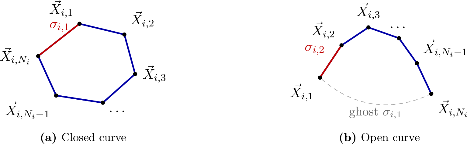
\[\Vec{X}_{i,j} := \begin{cases} \Gamma_i\left(\frac{j-1}{N_i}\right) & \qquad \text{if}\quad \Gamma_i\;\text{is closed},\\ \Gamma_i\left(\frac{j-1}{N_i-1}\right) & \qquad \text{if}\quad \Gamma_i\;\text{is open}. \end{cases}\] We let \[\sigma_{i,j} : [0,1] \ni t\mapsto (1-t)\Vec{X}_{i,j-1} + t\Vec{X}_{i,j} \in \mathbb{R}^{2}\qquad\text{for}\quad 1\leq j\leq N_i.\] From now on, we identify the image of \(\sigma_{i,j}\) with \(\sigma_{i,j}\) itself. Then, we define the approximate curve by \(\Gamma^h_{i} := \bigcup_{j=1}^{N_{i}}\sigma_{i,j}\). The discrete curve network is composed of the polygonal curves, i.e., \(\Gamma^h_{} := \bigcup_{i=1}^{I_S}\Gamma^h_{i}\); the ambient space \(\mathbb{R}^{2}\) is split into \(I_R\) polygonal regions \(\Omega_{r}^h\,(r\in\mathbb{N}_{\leq I_R})\), that is, \(\mathbb{R}^{2}\setminus\Gamma^h_{} = \bigcup_{r=1}^{I_R}\Omega_{r}^h\). If \(\Gamma^h_{i}\) is open, then the vertex \(\Vec{X}_{i,1}\) (resp. \(\Vec{X}_{i,N_{i}}\)) is supposed to be the start point (resp. endpoint) of the curve \(\Gamma^h_{i}\). Moreover, it is also supposed that the endpoints of an open curve in \(\mathbb{R}^{2}\) correspond to some triple junctions in the curve network \(\Gamma^h_{}\). Meanwhile, if \(\Gamma_i\) is closed, then it is alternatively assumed that \(\Vec{X}_{i,0} = \Vec{X}_{i,N_{i}}\) (see Figure 2).
We also define a discrete variant of the normal vector field on \(\Gamma^h_{i}\) by \[\Vec{\nu}^h_{i,j} := \frac{\left(\Vec{X}_{i,j} - \Vec{X}_{i,j-1}\right)^\perp}{r_{i,j}}\qquadfor\quad i\in\mathbb{N}_{\leq I_S}\quadand\quad 1\leq j\leq N_{i},\] where \(r_{i,j} := |\sigma_{i,j}| = \left|\Vec{X}_{i,j} - \Vec{X}_{i,j-1}\right|\), and for any vector \(\Vec{x}\in\mathbb{R}^2\), the symbol \(\Vec{x}^\perp\) denotes the vector which is obtained by rotating \(\Vec{x}\) by \(90^\circ\) clockwise. We let \(\phi_{i,j}\) be the outer angle of \(\Gamma^h_{i}\) at the vertex \(\Vec{X}_{i,j}\) and define a discrete variant of the curvature \(\varkappa\) by \[\kappa^h_{i,j} := \frac{\tan{\left(\frac{\phi_{i,j-1}}{2}\right) + \tan{\left(\frac{\phi_{i,j}}{2}\right)}}}{r_{i,j}}\qquadfor\quad i\in\mathbb{N}_{\leq I_S}\quadand\quad 1\leq j\leq N_{i}.\] Since \(x\approx\tan{x}\) as \(|x|\ll 1\), the quantity \(\kappa^h_{i,j}\) approximates the turning rate of the curve at the edge center \(\Vec{X}^*_{i,j}\) defined by \[\Vec{X}^*_{i,j} := \frac{\Vec{X}_{i,j-1} + \Vec{X}_{i,j}}{2}\qquadfor\quad i\in\mathbb{N}_{\leq I_S}\quadand\quad 1\leq j\leq N_{i},\] provided that \(N_{i}\) is taken so large that \(r_{i,j}\ll 1\), and hence \(\kappa^h_{i,j}\approx\tfrac{d\phi}{ds} = -\varkappa\), where \(s\) denotes the arc-length parameter on \(\Gamma_i\). Here the sign is opposite to the normal-direction curvature \(\varkappa\) of Section 2: the outer angle \(\phi_{i,j}\) is positive when \(\Gamma^h_{i}\) turns counter-clockwise, so \(\kappa^h_{i,j} > 0\) for a curve that is convex toward the region \(\Omega_{r_{i}^-}^h\), whereas \(\varkappa< 0\) there. We retain \(\kappa^h_{i,j}\) (the implemented quantity) as the right-hand side of the discrete Gibbs–Thomson rows below and absorb the sign into the jump ordering accordingly. Here, we stress that the index \(j\) of the vertices should start from \(1\) if \(\Gamma^h_{i}\) is open, and it should start from \(0\) if \(\Gamma^h_{i}\) is closed since we cannot define the outer angle at the endpoints of open curves.
Remark 6. In the previous work [39], the author considered open curves whose endpoints are not triple junctions and lie on the boundary of a half space. Moreover, he defined imaginary vertices to define the values of \(\kappa^h_{i,j}\) on the boundary of the half space. However, in the present model, triple junctions can evolve in time, and the curvature at these points does not make sense. The half-space setting is revisited in Section 7, where the wall endpoints become mobile contacts that meet the wall orthogonally and may coexist with evolving triple junctions.
Remark 7 (Curvature correction near triple junctions). For an open curve \(\Gamma^h_{i}\), the standard formula for \(\kappa^h_{i,j}\) uses the outer angles at both endpoints of the edge \(\sigma_{i,j}\), which are unreliable for the four edges adjacent to the triple junctions (\(j = 2, 3, N-1, N\) with \(N := N_{i}\)), since the outer angle is undefined at the junction vertices. By default the implementation re-evaluates the discrete curvature only at these four edges and only for the right-hand side of the Gibbs–Thomson rows 25 , using one-sided differences of the turning angle that do not involve the junction vertex, \[\begin{align} &\kappa^h_{i,2} \leftarrow \frac{\phi_{i,2}}{(\ell_2+\ell_3)/2}, \quad \kappa^h_{i,3} \leftarrow \frac{\phi_{i,2}+\phi_{i,3}}{\ell_2/2+\ell_3+\ell_4/2},\\ &\kappa^h_{i,N} \leftarrow \frac{\phi_{i,N-1}}{(\ell_{N-1}+\ell_N)/2}, \quad \kappa^h_{i,N-1} \leftarrow \frac{\phi_{i,N-2}+\phi_{i,N-1}}{\ell_{N-2}/2+\ell_{N-1}+\ell_N/2}, \end{align}\] with \(\ell_j := r_{i,j}\). This correction applies to open curves only; for closed curves the discrete curvature is used unchanged. It modifies neither the curvature stored for any other purpose nor the closed-curve rows, and it can be disabled, recovering the uncorrected scheme. The size of the deficit incurred without the correction, its behavior under refinement, and its confinement to the field accuracy near the junctions are quantified in Section 9.2.
6 Fully discrete scheme↩︎
In this section, we give a fully discrete scheme to approximate the interface evolution governed by 1 . To this end, given a smooth curve network \(\Gamma\), we first obtain the spatial discretization \(\Gamma^h_{}\) of \(\Gamma\) using the method introduced in Section 5. After that, we compute the normal velocity \(V\) of \(\Gamma^h_{}\) at each vertex, which is determined by 4 . Therefore, we are led to compute \(\mathbf{w}\) at each time step. In this paper, we adopt the charge simulation method (CSM) to solve the Dirichlet boundary problem 2 and 3 . We now explain a basic idea of the CSM.
Let \(\Phi\) be the fundamental solution to the Laplace equation in \(\mathbb{R}^2\), that is \[\Phi(\Vec{x}) := \frac{1}{2\pi}\log|\Vec{x}| \qquadfor\quad \Vec{x}\in\mathbb{R}^2\setminus\{\Vec{0}\}.\] Then, for \(r\in\mathbb{N}_{\leq I_R}\) and \(p\in\mathbb{N}_{\leq I_P}\), the approximate solution is defined by \[\label{eq:appsol} w^{(r)}_{p}(\Vec{x}) := c^{(r)}_{p} + \sum_{i\in \mathscr C_r^{-1}(r)}\sum_{j=1}^{N_{i}}Q^{(r)}_{p,i,j}\left\{\Phi\left(\Vec{x} - \Vec{y}^{(r)}_{i,j}\right) - \Phi\left(\Vec{x} - \Vec{z}^{(r)}_{i,j}\right)\right\} \qquadfor\quad \Vec{x}\in\mathbb{R}^2,\tag{15}\] where we recall that \(w^{(r)}_{p} := w_p\lfloor_{\Omega_{r}^h}\), the constant \(c^{(r)}_p\) is a region-wise additive constant (one per region \(r\) and phase \(p\), not shared across regions), and \(\Vec{y}^{(r)}_{i,j}\) and \(\Vec{z}^{(r)}_{i,j}\) are the charge points of the CSM, both placed outside \(\Omega_{r}\). Such a combination of fundamental solutions is well-known for its fast (for analytic data, exponential) convergence together with the attendant ill-conditioning of the collocation matrix in the literature [33]–[36].
Remark 8. The origin of construction for approximate solutions in 15 goes back to Murota [44] in which an invariant structure against affine transformations of the coordinate has been invoked in the definition of approximate solutions. Due to the appearance of one more unknown, the zero-sum condition on the unknowns has been imposed to solve a linear system. Therein, the dummy singular points \(\Vec{z}^{(r)}_{i,j}\) did not indeed appear in the representation of approximate solutions, and the use of this kind of points has been proposed by Sakakibara and Yazaki [45]. In their study, an area-preserving property has been encoded into a linear system instead of Murota’s zero-sum condition. This structure ensures invariance property of the approximate solution with respect to scale transformation (see [39]). We note that this invariant property is valid only in the planar case thanks to the logarithm of the fundamental solution.
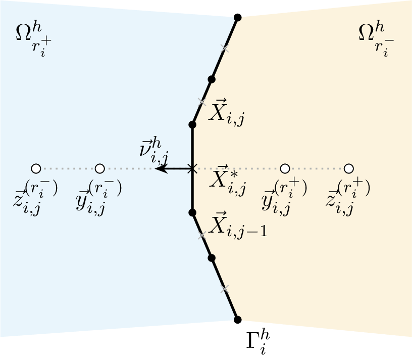
For each \(r\in\mathbb{N}_{\leq I_R}\), we let \[M_r := \sum_{i\in \mathscr C_r^{-1}(r)}\#\left\{\,edges of \Gamma^h_{i}\,\right\}\] be the total number of collocation points (edge centers) on \(\partial\Omega_{r}^h\), and let \[\label{eq:orientation} \Vec{\nu}^{\mathrm{out}}_{r,i,j} := o_{r,i}\,\Vec{\nu}^h_{i,j}, \qquad o_{r,i} := \begin{cases} +1 & r = r_{i}^-,\\ -1 & r = r_{i}^+,\end{cases}\tag{16}\] denote the unit normal of \(\Gamma^h_{i}\) pointing out of \(\Omega_{r}^h\) (note that \(\Vec{\nu}^h_{i,j}\) points from \(\Omega_{r_{i}^-}^h\) to \(\Omega_{r_{i}^+}^h\)). The charge points are then set as \[\label{eq:charge} \Vec{y}^{(r)}_{i,j} := \Vec{X}^*_{i,j} + \frac{1}{\sqrt{M_r}}\,\Vec{\nu}^{\mathrm{out}}_{r,i,j}\qquadand\qquad\Vec{z}^{(r)}_{i,j} := \Vec{X}^*_{i,j} + M_r^{\,\beta}\,\Vec{\nu}^{\mathrm{out}}_{r,i,j},\qquad \beta := \tfrac{3}{2},\tag{17}\] where the constant \(\beta\) has been chosen according to [39]. Both points lie on the same (outer) side of \(\Omega_{r}^h\): the principal point \(\Vec{y}^{(r)}_{i,j}\) at the short distance \(1/\sqrt{M_r}\), and the auxiliary point \(\Vec{z}^{(r)}_{i,j}\) far away at distance \(M_r^{\,\beta}\). It was shown in [39] that the approximate solution 15 satisfies the Neumann boundary condition 5 , i.e., \[\nabla\Phi\left(\Vec{x}-\Vec{y}^{(r)}_{i,j}\right)-\nabla\Phi\left(\Vec{x}-\Vec{z}^{(r)}_{i,j}\right) = O\left(\frac{1}{|\Vec{x}|^2}\right)\qquad\text{as}\quad |\Vec{x}|\to\infty,\] matching the far-field condition in 5 . When \(\partial\Omega_{r}^h\) has several connected components (for instance the exterior region of a configuration containing an isolated closed curve), the points 17 are placed component by component. Figure 3 illustrates this charge-simulation set-up near an interface curve \(\Gamma^h_{i}\).
Using these notations, we now explain how to determine the coefficients \(c^{(r)}_{p}\) and \(Q^{(r)}_{p,i,j}\). We note that the chemical potentials \(w^{(r)}_{p}\) sum up to zero for each \(r\in \mathbb{N}_{\leq I_R}\), so we only need to determine the coefficients for \(1 \leq p \leq I_P - 1\). Since the additive constant \(c^{(r)}_p\) is region-wise, each region contributes one constant per phase. Thus, the number of unknowns is equal to \[\label{eq:num-unknowns} n_{unk}:= (I_P - 1)\left\{\sum_{r=1}^{I_R}\left(\sum_{i\in \mathscr C_r^{-1}(r)}N_i + 1\right)\right\}.\tag{18}\] First, the Gibbs–Thomson law 3 is imposed on both sides of each curve. Recalling the discrete curvature \(\kappa^h_{i,j}\) together with its sign convention fixed in Section 5, the relation to be discretized reads \[\label{eq:GTL} w^{(r_{i}^\pm)}_{p_{i}^-} - w^{(r_{i}^\pm)}_{p_{i}^+} = \varsigma_{i}\,\kappa^h_i\quadon\quad\Gamma^h_{i}\quadfor\quad i\in\mathbb{N}_{\leq I_S}.\tag{19}\] Second, the continuity condition of the chemical potential across the curve network \(\Gamma\) 7 is given by \[\label{eq:CC} w^{(r_{i}^+)}_{p} = w^{(r_{i}^-)}_{p}\quadon\quad\Gamma^h_{i}\quadfor\quad i\in\mathbb{N}_{\leq I_S}\quadand\quad 1\leq p\leq I_P - 1.\tag{20}\]
We can directly calculate the normal derivative of the approximate solution 15 as follows: \[\nabla w^{(r)}_{p}(\Vec{x}) = \sum_{i\in \mathscr C_r^{-1}(r)}\sum_{j=1}^{N_{i}}Q^{(r)}_{p,i,j}\left\{\nabla\Phi\left(\Vec{x} - \Vec{y}^{(r)}_{i,j}\right) - \nabla\Phi\left(\Vec{x} - \Vec{z}^{(r)}_{i,j}\right)\right\},\] and the normal velocity \(v_{i,j}\) at the edge center \(\Vec{X}^*_{i,j}\) is computed from the motion law 4 , which gives the two equivalent representations: \[\label{eq:Vij} \left(\nabla w^{(r_{i}^+)}_{p_{i}^+} - \nabla w^{(r_{i}^-)}_{p_{i}^+}\right)\cdot\Vec{\nu}^h_{i,j} = -v_{i,j}\quadand\quad \left(\nabla w^{(r_{i}^+)}_{p_{i}^-} - \nabla w^{(r_{i}^-)}_{p_{i}^-}\right)\cdot\Vec{\nu}^h_{i,j} = v_{i,j}.\tag{21}\] In the implementation, we choose the second representation in 21 , i.e., from the phase \(p_{i}^-\) (\(= \mathscr R_p(r_{i}^-)\)) on both sides of \(\Gamma^h_{i}\).
Remark 9. The two representations in 21 coincide for an exact solution, which expresses the flux-balance (“motion-law”) consistency \[\left(\nabla w^{(r_{i}^+)}_{p_{i}^+} - \nabla w^{(r_{i}^-)}_{p_{i}^+}\right)\cdot\Vec{\nu}^h_{i,j} + \left(\nabla w^{(r_{i}^+)}_{p_{i}^-} - \nabla w^{(r_{i}^-)}_{p_{i}^-}\right)\cdot\Vec{\nu}^h_{i,j} = 0.\] This identity is a property expected of the continuous solution; it is not imposed as an independent row of the discrete linear system. Instead, the Gibbs–Thomson law is collocated on both adjacent regions of each curve (see 19 ), so that no separate motion-law row is assembled.
We need \((I_P - 1)\) more equations to determine the coefficients. To this end, we take the area-preserving condition for each phase into account (see Proposition 2). Namely, we require that \[0 = \frac{d}{dt}\sum_{r\in \mathscr R_p^{-1}(p)}\left|\Omega_{r}(t)\right| = -\sum_{r\in \mathscr R_p^{-1}(p)}\int_{\partial\Omega_{r}}V_{in}(r)\,\mathrm{d}\mathcal{H}^{1}\quadfor\quad 1\leq p \leq I_P - 1,\] where \(V_{in}(r)\) denotes the inward normal velocity at the boundary \(\partial\Omega_{r}\). We discretize the integration over the boundary \(\partial\Omega_{r}\) by the sum of the integrals over the edges \(\sigma_{i,j}\). Then, we obtain \[\label{eq:AP} \sum_{r\in \mathscr R_p^{-1}(p)}\left(\sum_{\substack{i\in \mathscr C_r^{-1}(r)\\ r = r_{i}^+}}\sum_{j=1}^{N_{i}}v_{i,j}r_{i,j} + \sum_{\substack{i\in \mathscr C_r^{-1}(r)\\ r = r_{i}^-}}\sum_{j=1}^{N_{i}}-v_{i,j}r_{i,j}\right) = 0\quadfor\quad 1\leq p\leq I_P - 1.\tag{22}\] The condition 22 constrains only the change of area. The area surrounded by the oriented boundary circuit \(\partial\Omega_{r}^h\) is computed by the shoelace formula: \[\label{eq:shoelace-area} \left|\Omega_{r}^h\right| = \frac{1}{2}\left|\, \sum_{i\in \mathscr C_r^{-1}(r)} o_{r,i} \sum_{j=1}^{N_{i}} \Vec{X}_{i,j-1}\times\Vec{X}_{i,j} \,\right|, \qquad \Vec{a}\times\Vec{b} := a_1 b_2 - a_2 b_1 ,\tag{23}\] where the orientation sign \(o_{r,i}\) of 16 traverses each incident curve in the direction consistent with \(\partial\Omega_{r}^h\); adjacent curves share their triple-junction endpoints, so the circuit closes with no connecting edges. Differentiating 23 in time reproduces, to leading order, the left-hand side of 22 : the linear system enforces \(\tfrac{d}{dt}|\Omega_{r}(t)|=0\) at the velocity level, while 23 is the polygonal area whose residual drift \(E_A\) is reported in Section 9. Here, we note that the inward normal velocity \(V_{in}(r)\) at the boundary \(\partial\Omega_{r}\) is given by \[V_{in}(r) = \begin{cases} v_{i,j}\qquad&for\quad r = r_{i}^+,\\ -v_{i,j}\qquad&for\quad r = r_{i}^-. \end{cases}\] To compute the above \(v_{i,j}\), we can use the formulae 21 .
Finally, we represent the formulae 19 , 20 , and 22 as a linear system of the coefficients \(c^{(r)}_{p}\) and \(Q^{(r)}_{p,i,j}\). To this end, we introduce the following notations: \[\begin{align} G^{(r)}_{(c_1,\ell),(c_2,j)} &:= \Phi\left(\Vec{X}^*_{c_1,\ell} - \Vec{y}^{(r)}_{c_2,j}\right) - \Phi\left(\Vec{X}^*_{c_1,\ell} - \Vec{z}^{(r)}_{c_2,j}\right),\\ \Vec{H}^{(r)}_{(c_1,\ell),(c_2,j)} &:= \nabla\Phi\left(\Vec{X}^*_{c_1,\ell} - \Vec{y}^{(r)}_{c_2,j}\right) - \nabla\Phi\left(\Vec{X}^*_{c_1,\ell} - \Vec{z}^{(r)}_{c_2,j}\right), \end{align}\] for \(r\in\mathbb{N}_{\leq I_R}\), \(c_1,\,c_2\in\mathbb{N}_{\leq I_S}\), \(\ell\in\mathbb{N}_{\leq N_{c_1}}\), and \(j\in\mathbb{N}_{\leq N_{c_2}}\).
Then, we obtain the following linear system.
\[\tag{24} \boldsymbol{[Gibbs--Thomson law]} For every i\in\mathbb{N}_{\leq I_S}, k\in\mathbb{N}_{\leq N_{i}}, and each side r_{i}^\pm\in\{r_{i}^-,r_{i}^+\}, it holds that \begin{equation}\tag{25} c^{(r_{i}^\pm)}_{p_{i}^-} - c^{(r_{i}^\pm)}_{p_{i}^+} + \sum_{\ell\in \mathscr C_r^{-1}(r_{i}^\pm)}\sum_{j=1}^{N_{\ell}}\left(Q^{(r_{i}^\pm)}_{p_{i}^-,\ell,j} - Q^{(r_{i}^\pm)}_{p_{i}^+,\ell,j}\right) G^{(r_{i}^\pm)}_{(i,k),(\ell,j)} = \varsigma_{i}\kappa^h_{i,k}. \end{equation} \boldsymbol{[Continuity condition]} For every i\in\mathbb{N}_{\leq I_S}, k\in\mathbb{N}_{\leq N_{i}}, and 1\leq p\leq I_P - 1, it holds that \begin{equation}\tag{26} c^{(r_{i}^+)}_{p} - c^{(r_{i}^-)}_{p} + \sum_{\ell\in \mathscr C_r^{-1}(r_{i}^+)}\sum_{j=1}^{N_{\ell}}Q^{(r_{i}^+)}_{p,\ell,j}G^{(r_{i}^+)}_{(i,k),(\ell,j)} - \sum_{\ell\in \mathscr C_r^{-1}(r_{i}^-)}\sum_{j=1}^{N_{\ell}}Q^{(r_{i}^-)}_{p,\ell,j}G^{(r_{i}^-)}_{(i,k),(\ell,j)} = 0. \end{equation} \boldsymbol{[Area-preserving condition]} For every 1\leq p\leq I_P-1, it holds that \begin{equation}\tag{27} \sum_{r\in \mathscr R_p^{-1}(p)}\left(\sum_{\substack{i\in \mathscr C_r^{-1}(r)\\ r = r_{i}^+}}\sum_{j=1}^{N_{i}} r_{i,j}\, v_{i,j} - \sum_{\substack{i\in \mathscr C_r^{-1}(r)\\ r = r_{i}^-}}\sum_{j=1}^{N_{i}} r_{i,j}\, v_{i,j}\right) = 0, \end{equation} where the single normal velocity v_{i,j} is taken in the p_{i}^--representation (the second identity of \eqref{eq:Vij}): \begin{equation*} v_{i,j} = \left(\sum_{\ell\in \mathscr C_r^{-1}(r_{i}^+)}\sum_{k=1}^{N_{\ell}}Q^{(r_{i}^+)}_{p_{i}^-,\ell,k}\Vec{H}^{(r_{i}^+)}_{(i,j),(\ell,k)} - \sum_{\ell\in \mathscr C_r^{-1}(r_{i}^-)}\sum_{k=1}^{N_{\ell}}Q^{(r_{i}^-)}_{p_{i}^-,\ell,k}\Vec{H}^{(r_{i}^-)}_{(i,j),(\ell,k)}\right) \cdot\Vec{\nu}^h_{i,j}. \end{equation*}\]
The rows 25 , 26 , and 27 assemble into a linear system \(A\Vec{q} = \Vec{b}\) for the unknown vector \(\Vec{q}\in\mathbb{R}^{n_{unk}}\) collecting the region-wise coefficients \(Q^{(r)}_{p,i,j}\) and constants \(c^{(r)}_p\) (\(1\le p\le I_P-1\)). Since the Gibbs–Thomson law is collocated on both regions of each curve and the additive constants are region-wise, this system is not square: it is in general overdetermined and rank-deficient, and we do not solve it by a direct square solve. Instead, we treat it as a constrained least-squares problem in which the area-preserving rows are imposed exactly.
Let \(C\Vec{q} = \Vec{0}\) denote the \((I_P-1)\) area-preserving rows 27 , and let \(A_1\Vec{q} = \Vec{b}_1\) denote the remaining Gibbs–Thomson 25 and continuity 26 rows. We enforce \(C\Vec{q}=\Vec{0}\) as a hard constraint by the orthogonal projection onto its null space: \[\label{eq:proj} P := I - C^\top\left(CC^\top\right)^{-1}C,\tag{28}\] and we solve the projected least-squares problem: \[\label{eq:pcgls} \min_{\Vec{y}} \left\|A_1 P\Vec{y} - \Vec{b}_1\right\|_2^2, \qquad \Vec{q} := P\Vec{y},\tag{29}\] by the conjugate-gradient least-squares (CGLS) iteration. By construction, \(C\Vec{q} = CP\Vec{y} = \Vec{0}\) holds to machine precision, and thus the discrete area-preserving condition 27 is satisfied at the level of the reconstructed velocity field independently of the residual of 29 . The Gibbs–Thomson and continuity rows are then satisfied in the least-squares sense.
The normal velocities \(v_{i,j}\) are computed at the edge centers \(\Vec{X}^*_{i,j}\), whereas the curve is advanced by moving its vertices \(\Vec{X}_{i,j}\). We therefore transfer the edge data to the vertices by averaging the adjacent edge normals and tangents. Define the (unnormalized) vertex normal and tangent \[\overline{\Vec{\nu}}_{i,j} := \frac{\Vec{\nu}^h_{i,j} + \Vec{\nu}^h_{i,j+1}}{2\cos\left(\frac{\phi_{i,j}}{2}\right)}, \qquad \overline{\Vec{\tau}}_{i,j} := \frac{\Vec{\tau}_{i,j} + \Vec{\tau}_{i,j+1}}{2\cos\left(\frac{\phi_{i,j}}{2}\right)},\] where \(\Vec{\tau}_{i,j}\) is the unit tangent of the edge \(\sigma_{i,j}\). Each vertex is then advanced by the normal velocity along \(\overline{\Vec{\nu}}_{i,j}\) together with a tangential redistribution velocity \(T_{i,j}\), which will be determined by the uniform distribution method (UDM) below, along \(\overline{\Vec{\tau}}_{i,j}\): \[\label{eq:evolve} \Vec{X}^{(n+1)}_{i,j} = \Vec{X}^{(n)}_{i,j} + \Delta t V^{(n)}\qquad\text{with}\quad V^{(n)} := v_{i,j}\,\overline{\Vec{\nu}}_{i,j} + T_{i,j}\,\overline{\Vec{\tau}}_{i,j}.\tag{30}\] For an open curve the two endpoints (\(j=1\) and \(j=N_{i}\)) are held fixed at this stage (their velocity is set to zero) and are subsequently relocated by the triple-junction correction below; for a closed curve all vertices are advanced by 30 . Here, \(\Delta t > 0\) is a time step size; in the numerical experiments, we take \(\Delta t = c / N^2\) with a fixed constant \(c\) (typically \(c\in[0.01, 0.5]\)), where \(N\) is the number of vertices per curve.
Remark 10. The region-wise constants \(c^{(r)}_p\) are not shared across regions. Their differences across each curve are fixed by the continuity rows 26 , and the remaining gauge freedom (a global additive constant per phase) is harmless for the velocity reconstruction, which depends only on the gradients \(\nabla w^{(r)}_{p}\). The constrained least-squares 29 selects a representative consistent with all rows.
To avoid mesh degeneration, we redistribute the vertices along the curve by the tangential velocity \(T_{i,j}\) of 30 ; since this motion is tangential, it does not change the geometric evolution. To this end, we follow the strategy of [39], although we modify it so that each curve may be open. Fix a polygonal curve \(\Gamma^h_{i}\) with \(N := N_{i}\) edges, write \(\ell_j := r_{i,j}\) for the edge lengths, \(L^h_{} := \sum_{j=1}^{N_i} \ell_j\) for its length, and \[\dot{L}^h := \sum_{j} \kappa^h_{i,j}\, v_{i,j}\,\ell_j \approx \int_\Gamma \varkappa V\,\mathrm{d}\mathcal{H}^{1} = \dot{L}\] for the discrete derivative of length, where the sum runs over the real edges (\(j=2,\dots,N\) for an open curve, \(j=1,\dots,N\) for a closed one). The redistribution drives the edge lengths toward the uniform value \(L/N\) (resp.\(L/(N-1)\) for an open curve), where \(L\) denotes the length of the curve which is supposed to be approximated by the polygonal curve \(\Gamma^h_{i}\). We briefly explain its procedure. For a closed curve, set \[\psi_j := \frac{\dot{L}^h}{N} - v_{i,j}\sin\!\tfrac{\phi_{i,j}}{2} - v_{i,j-1}\sin\!\tfrac{\phi_{i,j-1}}{2} + \left(\frac{L^h}{N} - \ell_j\right) 10 N \qquad\text{with}\quad \Psi_j := \sum_{m=1}^{j}\psi_m,\] and define
\[T_{i,j} := \frac{\Psi_j + C}{\cos\tfrac{\phi_{i,j}}{2}}\qquad\text{with}\quad C := -\sum_j \frac{\Psi_j}{\cos\tfrac{\phi_{i,j}}{2}}\Big/\sum_j \frac{1}{\cos\tfrac{\phi_{i,j}}{2}}.\] Here, \(C\) is chosen so that the redistribution closes up around the loop.
For an open curve, the endpoint tangential velocities are fixed, i.e., \(T_{i,1} = T_{i,N} = 0\), and the interior values solve the bidiagonal least-squares system: \[\begin{gather} -\cos\!\tfrac{\phi_{i,j}}{2}\,T_{i,j} + \cos\!\tfrac{\phi_{i,j+1}}{2}\,T_{i,j+1}\\ = \frac{\dot{L}^h}{N-1} + \left(\frac{L^h}{N-1} - \ell_{j+1}\right)10 N - v_{i,j}\sin\!\tfrac{\phi_{i,j+1}}{2} - v_{i,j-1}\sin\!\tfrac{\phi_{i,j}}{2} \end{gather}\] for \(2\leq j\leq N-1\), which we solve by CGLS. In both cases the factor \(10N\) is an implementation parameter controlling the strength of the equi-distribution.
The triple junctions are updated geometrically, not as rows of the linear system 25 , 26 , and 27 . During the free curve update, the endpoints of each open curve are held fixed, while all interior vertices are advanced by 30 . For each \(k\in\mathbb{N}_{\leq I_T}\), let \(\Vec{a}_1,\Vec{a}_2,\Vec{a}_3\) denote the updated interior vertices adjacent to the junction \(\mathcal{T}_{k}\) on its three incident curves. We compute a new common junction position \(\Vec{p}^*_k\) such that the directions \(\Vec{a}_m-\Vec{p}^*_k\,(m=1,2,3)\) pairwise enclose the equilibrium angles (\(120^\circ\) in the equal-tension case). The point \(\Vec{p}^*_k\) is obtained by a damped, regularized Gauss–Newton iteration applied to the three angle-cosine residuals, initialized at the centroid of \(\Vec{a}_1,\Vec{a}_2,\Vec{a}_3\). The corresponding endpoint of every incident curve is then reset to this same point (Figure 4). Finally, the geometric quantities (edges, normals, outer angles, and the discrete curvature) of the affected curves are recomputed from the corrected vertices according to the procedure explained in Section 5. Since closed curves have no triple-junction endpoints, they are advanced by 30 with all of their vertices updated, without any endpoint correction. We stress that the Herring–Young condition is enforced here as a geometric correction.

7 Extension to Neumann boundary problem↩︎
So far, we have explained the implementation of the fully discrete scheme in the whole space \(\mathbb{R}^{2}\). In this section, we extend the proposed scheme to the half space \(\mathbb{H}\) with boundary contacts.
7.1 Half-space Neumann problem↩︎
First, we introduce a target problem whose solution will be approximated by our proposed scheme. Let \((\Vec{e}_1,\Vec{e}_2)\) be the standard basis of \(\mathbb{R}^{2}\). We consider the system 1 in the half space \(\mathbb{H}\) with the boundary wall \(\mathcal{W}\) defined by: \[\mathbb{H} := \left\{\Vec{x} = (x_1,x_2)^{\top} \in\mathbb{R}^{2} \biggm| x_2 > 0\right\}\quad\text{and}\quad \mathcal{W}:= \partial\mathbb{H} = \left\{\Vec{x} = (x_1,x_2)^\top\in\mathbb{R}^2 \biggm| x_2 = 0\right\}.\] The governing system is 1 with \(\mathbb{R}^2\) replaced by \(\mathbb{H}\), augmented by the wall condition: \[\label{eq:hs-neumann} \nabla\mathbf{w}(\cdot,t)\,\Vec{\nu}_{\mathcal{W}} = \mathbf{0}\qquadon\quad\mathcal{W},\quad t>0,\tag{31}\] where \(\Vec{\nu}_{\mathcal{W}} = -\Vec{e}_2\) is the outward unit normal vector to \(\mathbb{H}\), which is constant in the half-space case. An open curve may now end either at a triple junction (as in Section 6) or at the Neumann boundary. In the latter case, the endpoint can slide along \(\mathcal{W}\) (mobile) and is required to meet the boundary orthogonally, \[\label{eq:hs-ortho} \Vec{\mu}_i\cdot\Vec{e}_1 = 0\qquadat a boundary contact of \Gamma_i,\tag{32}\] i.e.,the interface tangent is vertical there (\(90^\circ\) contact). We stress that 32 is a prescribed neutral contact condition of the present model, which is imposed independently of the Neumann condition 31 , which constrains the chemical potential. The triple-junction force balance (the Herring–Young law, Remark 4) is retained unchanged.
Remark 11. In the two-phase case with \(d = 2,\,3\), local well-posedness of the underlying problem in a smooth bounded domain with the pure Neumann boundary condition 31 and ninety-degree angle contact condition 32 has been established by Abels, Rauchecker, and Wilke [46]. For a stability analysis of stationary solutions to the same flow in the case \(d = 2\), we refer the reader to Garcke and Rauchecker [47]. We refer the reader to Hensel and Stinson [48] for weak solutions in the case \(d = 2,\,3\) with constant contact angle condition.
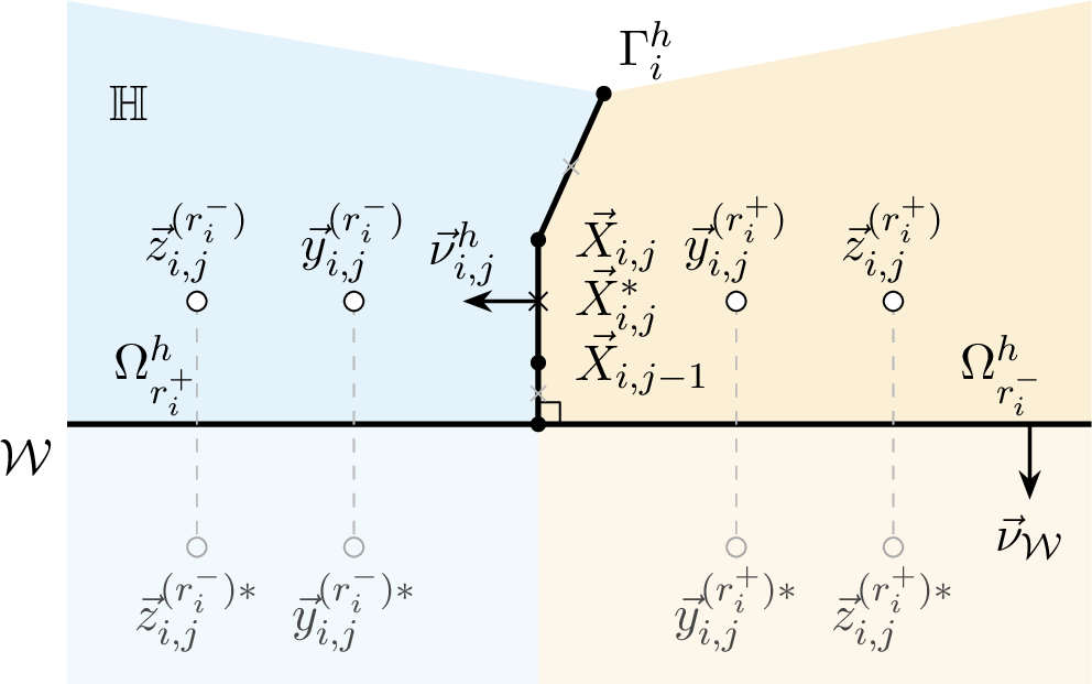
For a source point \(\Vec{q} = (q_1,q_2)^\top\), let its mirror image across the boundary be \[\label{eq:hs-mirror} \Vec{q}^\ast := (q_1,\; - q_2)^\top,\tag{33}\] and define the half-space (Neumann) fundamental solution by superposing the source and its image with equal sign, \[\label{eq:hs-image} \Phi_{\mathcal{W}}(\Vec{x},\Vec{q}) := \Phi(\Vec{x}-\Vec{q}) + \Phi(\Vec{x}-\Vec{q}^\ast),\tag{34}\] where we recall that \(\Phi\) is the fundamental solution to the Laplace equation in \(\mathbb{R}^{2}\). On the boundary, the distances from \(\Vec{q}\) and \(\Vec{q}^\ast\) coincide, i.e., \(|\Vec{x}-\Vec{q}| = |\Vec{x}-\Vec{q}^\ast|\) holds for \(\Vec{x}\) with \(x_2 = 0\), and the normal derivative is \[\label{eq:hs-noflux} \frac{\partial\Phi_{\mathcal{W}}}{\partial x_2}(\Vec{x},\Vec{q}) = \frac{1}{2\pi}\left[\frac{x_2-q_2}{|\Vec{x}-\Vec{q}|^2} + \frac{x_2 + q_2}{|\Vec{x}-\Vec{q}^\ast|^2}\right] = 0\qquadon\quad x_2 = 0,\tag{35}\] since on \(\mathcal{W}\) the two numerators are \(x_2-q_2 = -q_2\) and \(x_2 + q_2 = q_2\) while the denominators are equal. Hence, any potential built from \(\Phi_{\mathcal{W}}\) satisfies the homogeneous Neumann condition 31 on the boundary exactly, with no additional unknowns.
7.2 Fully discrete scheme for half-space Neumann problem↩︎
In the CSM, the approximate solution 15 is retained with \(\Phi\) replaced by \(\Phi_{\mathcal{W}}\), namely, the scalar and vector blocks remain the differences: \[\begin{align} \label{eq:hs-G} G^{(r)}_{(c_1,\ell),(c_2,j)} &= \Phi_{\mathcal{W}}(\Vec{X}^*_{c_1,\ell},\Vec{y}^{(r)}_{c_2,j}) - \Phi_{\mathcal{W}}(\Vec{X}^*_{c_1,\ell},\Vec{z}^{(r)}_{c_2,j}),\\ \Vec{H}^{(r)}_{(c_1,\ell),(c_2,j)} &= \nabla\Phi_{\mathcal{W}}(\Vec{X}^*_{c_1,\ell},\Vec{y}^{(r)}_{c_2,j}) - \nabla\Phi_{\mathcal{W}}(\Vec{X}^*_{c_1,\ell},\Vec{z}^{(r)}_{c_2,j}),\nonumber \end{align}\tag{36}\] where \(\nabla\) is applied to the field point \(\Vec{X}^*_{c_1,\ell}\). The charge-point placement, however, differs from 17 as follows: \[\label{eq:hs-source} \Vec{y}^{(r)}_{i,j} := \Vec{X}^*_{i,j} + \alpha\,r_{i,j}\,\Vec{\nu}^{\mathrm{out}}_{r,i,j},\qquad \Vec{z}^{(r)}_{i,j} := \Vec{X}^*_{i,j} + M_r^{3/2}\,\Vec{\nu}^{\mathrm{out}}_{r,i,j},\tag{37}\] i.e.,the principal source sits at a local-edge offset \(\alpha\,r_{i,j}\) (with \(\alpha\) an implementation parameter, \(\alpha=1.5\) in the runs) rather than at the \(1/\sqrt{M_r}\) distance of 17 ; the auxiliary source keeps the \(M_r^{3/2}\) far placement, and the principal-minus-dummy structure of 36 is retained. The local scaling \(\alpha\,r_{i,j}\) (rather than the global \(1/\sqrt{M_r}\)) is used because the orthogonal wall contact makes the edge lengths strongly non-uniform along each curve; anchoring the principal source to the local edge length keeps it at a fixed multiple of the local discretization scale, whereas a single global offset would sit at very different relative distances from the fine and coarse edges.
Remark 12. For the structure of fundamental solutions 34 , we have followed the previous work [39] to force the approximate solution to satisfy the pure Neumann boundary condition on \(\partial\mathbb{H} = \mathcal{W}\).
In Figure 5, we visualize this half-space charge-simulation construction near the Neumann wall \(\mathcal{W}\). A polygonal curve \(\Gamma^h_{i}\) contacts the boundary orthogonally at a mobile contact fulfilling 32 ; in this case, we have \(\Vec{\nu}_{\mathcal{W}}=-\Vec{e}_2\). Each region is represented, as in the whole space, by charge points held off the curve on the side outside that region: a principal point \(\Vec{y}^{(r)}_{i,j}\) at the near offset \(\alpha\,r_{i,j}\) and an auxiliary point \(\Vec{z}^{(r)}_{i,j}\) at the far distance \(M_r^{3/2}\) as in 37 . The half-space fundamental solution \(\Phi_{\mathcal{W}}\) in 34 superposes each charge with its wall mirror image \(\Vec{y}^{(r)\ast}_{i,j},\Vec{z}^{(r)\ast}_{i,j}\) reflected across \(\mathcal{W}\) as in 33 , using an equal sign, which enforces the homogeneous Neumann condition on \(\mathcal{W}\) exactly as in 35 .
7.3 Two distinct solves: charge field and constrained velocity↩︎
7.3.0.1 Charge-field solve.
The coefficients \(c^{(r)}_p\) and \(Q^{(r)}_{p,i,j}\) are obtained from the collocation system of Section 6 with the imaged blocks 36 and the placement 37 . Writing \(A_1\) for the two-sided Gibbs–Thomson 25 and continuity 26 rows (right-hand side \(\Vec{b}_1\)) and \(C\) for the aggregate per-phase area rows 27 (one per bounded phase, \(I_P-1\) in total), the half-space solve reads \[\label{eq:hs-charge} \min_{\Vec{q}}\;\left\{\bigl\|A_1\Vec{q}-\Vec{b}_1\bigr\|_2^2 + \lambda_D\,W_D^2\,\bigl\|D\Vec{q}\bigr\|_2^2\biggm|C\Vec{q}=\Vec{0}\right\}\tag{38}\] with the constraint enforced exactly by the orthogonal projection 28 . The block \(D\) collects, per collocation edge, the flux-balance residual: the inconsistency between the two phase representations of the normal velocity 21 . This block is the departure from the whole-space scheme, which assembles no motion-law row (Remark 9). It is penalized rather than enforced, because the Neumann wall and its mobile contacts couple the interface flux to the boundary while the collocation system is already rank-deficient; the weight \(\lambda_D=0.1\) keeps the Gibbs–Thomson/continuity fit dominant without ignoring the residual, and \(W_D\) rescales the rows of \(D\) to the magnitude of \(A_1\) so that \(\lambda_D\) acts as a dimensionless relative weight. From the reconstructed field the edge-center normal velocities \(v_{i,j}\) are recovered as in 21 .
7.3.0.2 Constrained velocity solve.
A separate reconstruction stage takes the \(v_{i,j}\) as data and produces the vertex velocities and the endpoint motion; the wall and junction constraints below are not rows of the charge-field system. Each open-curve endpoint is a triple-junction node, a wall contact (\(x_2=0\)), or free; let \(I_W\), \(I_T\), and \(I_A\) count the mobile wall contacts, the trivalent junctions, and the area hard rows. The unknowns are the per-curve vertex velocities \(\Vec{v}_{i,j}\) and, for each triple junction \(t\), a shared junction velocity \(\Vec{V}_t\in\mathbb{R}^{2}\) and a scalar angular rate \(\omega_t\) (every junction-incident endpoint moves with \(\Vec{V}_t\)). The stage minimizes the fidelity/redistribution objective of Section 7.4 under the hard wall, junction, and area rows: \[\label{eq:hs-kkt} \boxed{\; \begin{align} \min_{\{\Vec{v}_{i,j}\},\,\{\Vec{V}_t,\omega_t\}}\; & \left\{\textstyle\sum_i\bigl(\lVert F_i\rVert_2^2 + \lVert R_i\rVert_2^2\bigr) + \gamma\lVert G\rVert_2^2 + \lambda_{\mathrm{reg}}\lVert\Vec{v}\rVert_2^2\right\} && \text{\small(soft rows; \S\ref{sec:subsec:hs-manifold})}\\[-1pt] \text{s.t.}\; & \Vec{v}_c\cdot\Vec{e}_2=0,\;\; (\Vec{v}_c-\Vec{v}_a)\cdot\Vec{e}_1=0 && \text{\small(wall contact, 90^\circ)}\\ & \tfrac{1}{\ell}(R_{90}\Vec{t}_{\mathrm{away}})\cdot(\Vec{v}_a-\Vec{V}_t)=\omega_t && \text{\small(junction incidence, 120^\circ)}\\ & \tfrac{\mathrm{d}}{\mathrm{d}t}\sum_{r\in\mathscr R_p^{-1}(p)}\lvert\Omega_{r}^h(t)\rvert=0 && \text{\small(bounded region)} \end{align}\;}\tag{39}\] Here \(\Vec{v}_c\) is a contact velocity, \(\Vec{v}_a\) that of the adjacent interior vertex, \(\ell\) the junction-to-neighbor distance, \(\Vec{t}_{\mathrm{away}}\) the unit tangent pointing away from the junction, and \(R_{90}\) the \(90^\circ\) rotation. Table 1 lists the rows: the two wall rows are the velocity-level form of 32 ; the shared \(\omega_t\) across a junction’s three incidences is an equal-angular-rate condition preserving the \(120^\circ\) balance of Remark 4; the soft families \(F_i,R_i,G\) are defined in Section 7.4; and a phase composed of several bounded regions is assigned one aggregate row \(C\Vec{q}=\Vec{0}\) of 38 . The reconstructed \(\Vec{v}_{i,j}\) advance the vertices, and the junction-incident endpoints move with their \(\Vec{V}_t\). The hard rows sum to \[\label{eq:hs-count} n_c = I_A + 2\,I_W + 3\,I_T ,\tag{40}\] with \(I_A\) one row per constrained bounded region (or per multi-region phase in the aggregate case). In the assembled examples, each phase occupies a single region, so \(I_A = I_R-1 = I_P-1\) and 40 gives \(n_c = 18\) for the four-phase configuration of Section 9.7.
| rows | type | definition | count | role |
|---|---|---|---|---|
| wall contact | hard | \(\bv{v}_c\cdot\bv{e}_2=0,\;(\bv{v}_c-\bv{v}_a)\cdot\bv{e}_1=0\) | \(2I_W\) | \(90^\circ\) contact [eq:hs-ortho] |
| junction incidence | hard | \(\tfrac{1}{\ell}(\rotation\bv{t}_{\mathrm{away}})\cdot(\bv{v}_a-\bv{V}_t)=\omega_t\) | \(3I_T\) | shared \(\omega_t\) keeps \(120^\circ\) |
| area rate | hard | \(\tfrac{\mathrm{d}}{\mathrm{d}t}\lvert\regionDiscrete{r}(t)\rvert=0\) | \(I_A\) | phase-area conservation |
| fidelity \(F_i\) | soft, \(1\) | \(\widehat{\bv{n}}_{i,k}\cdot\bv{v}_{i,k}=v^n_{i,k}\) | per vertex | normal-motion fidelity |
| compatibility \(G\) | soft, \(\sqrt{\gamma}\) | \(\bv{n}_{i,\mathrm{adj}}\cdot\bv{V}_t=v^n_{i,\mathrm{adj}}\) | per incidence | junction–arc coupling |
| equidistribution \(R_i\) | soft, \(\beta_0\) | [eq:hs-equidist] | per edge | tangential mesh regularity |
| Tikhonov | soft, \(\lambda_{\mathrm{reg}}\) | \(\lambda_{\mathrm{reg}}\lVert\bv{v}\rVert_2^2\) | once | positive-definite block |
4.5pt
7.3.0.3 Region closure at the wall.
The area-rate row needs the region’s oriented boundary polygon, assembled by an incidence-driven traversal that chains the boundary curves through their shared junction nodes and closes a wall-touching region with a wall chord between its two contacts. A bounded region with three wall contacts or with disjoint wall intervals cannot be closed unambiguously and is excluded; the validated class is exactly that of Section 7: one contiguous wall interval, bounded by two consecutive contacts, per bounded wall-touching region.
7.4 Tangential redistribution and on-manifold endpoint update↩︎
The hard rows of 39 constrain the velocities to be tangent to the wall and junction constraint manifolds; the endpoint update below then advances the positions on those manifolds through explicit charts (Figure 6). The \(90^\circ\) and \(120^\circ\) angles therefore hold to machine precision at every stage of the time step, independently of the step size.
7.4.0.1 Soft rows: fidelity and redistribution.
The soft rows of 39 form three least-squares families (Table 1):
Fidelity \(F_i\) (weight \(1\)): \(\widehat{\Vec{n}}_{i,k}\!\cdot\Vec{v}_{i,k}=v^n_{i,k}\) pins the normal component of each owned velocity to the reconstructed raw value (\(k=2,\dots,N-1\) on an open curve, every vertex on a closed one).
Compatibility \(G\) (weight \(\sqrt\gamma\), \(\gamma=1\)): \(\Vec{n}_{i,\mathrm{adj}}\!\cdot\Vec{V}_t=v^n_{i,\mathrm{adj}}\), one row per junction incidence, ties \(\Vec{V}_t\) to the incident normal velocities as strongly as each vertex honors its own.
Equidistribution \(R_i\) (weight \(\beta_0=10\)): on each curve the edge rates are driven toward uniformity, \[\label{eq:hs-equidist} \dot{\ell}_e - \frac{\dot{L}}{N_e} = \beta\left(\bar\ell - \ell_e\right),\qquad \bar\ell := \frac{L}{N_e},\tag{41}\] with \(\ell_e\) the edge lengths, \(L\) the curve length, \(N_e\) the number of edges (\(N-1\) open, \(N\) closed), and \(\beta=\beta_0\,\max_i N_i\) (\(\beta_0\) dimensionless, distinct from the exponent in 17 ). This rate is fast enough to keep the mesh regular and slow enough not to overwhelm the normal motion.
A fixed Tikhonov term \(\lambda_{\mathrm{reg}}\lVert\Vec{v}\rVert_2^2\) (\(\lambda_{\mathrm{reg}}=10^{-8}\)) makes the owned-vertex block positive-definite without perturbing the physical velocity. All are penalties, not hard equalities: 41 is the velocity-level, curve-wide analogue of the uniform-distribution method of Section 6, and the solve targets the raw normal velocity while selecting a tangential redistribution under the hard rows; the diagnostics of Section 9.7 confirm that the constrained evolution remains consistent with the intended normal flow.
7.4.0.2 On-manifold endpoint charts.
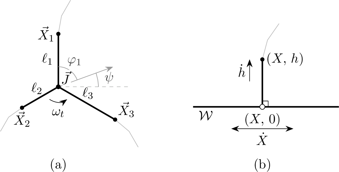
This update replaces the post-hoc geometric triple-junction correction of Section 6. Each trivalent junction is equipped with a chart \((\Vec{J},\psi,\{\varphi_k,\ell_k\}_{k=1}^3)\), consisting of a junction point, a shared frame angle, and, per incident ray, a fixed angular offset and an evolving length (Figure 6 (a)); the incident endpoint is reconstructed as \[\label{eq:hs-tjchart} \Vec{X}_k = \Vec{J} + \ell_k\bigl(\cos(\psi+\varphi_k),\,\sin(\psi+\varphi_k)\bigr);\tag{42}\] the offsets \(\varphi_k\) being fixed, the \(120^\circ\) balance is exact for all \(t\). Each wall contact is equipped with a chart \((X,h)\) (Figure 6 (b)), \[\label{eq:hs-wallchart} \Vec{X}_{\mathrm{contact}} = (X,\,0)^\top,\qquad \Vec{X}_{\mathrm{adj}} = (X,\,h)^\top,\tag{43}\] so the contact edge is vertical and the \(90^\circ\) angle is exact. A two-stage Heun update advances the chart coordinates (a predictor at \(t\), a corrector at the tentative state, the rates averaged); the constraints 42 –43 hold to machine precision at each stage. The update is formally second order (Heun/RK2); we do not measure a temporal convergence rate and do not claim unconditional stability.
7.4.0.3 Adaptive time step.
Unlike the whole-space runs of Section 6, which use the fixed rule \(\Delta t=c\,N^{-2}\), we choose the time step adaptively in the half-space runs as \[\label{eq:hs-dt-rule} \Delta t = \min\left\{c_{\mathrm{CFL}}\,\frac{\min_{i,j}\ell_{i,j}}{\max_\Gamma|V|},\;\Delta t_{\max}\right\},\tag{44}\] where \(\min_{i,j}\ell_{i,j}\) is the smallest polygonal edge length in the network, \(\max_\Gamma|V|\) the maximum discrete normal speed, \(c_{\mathrm{CFL}}>0\) a Courant constant, and \(\Delta t_{\max}\) a cap (in the runs \(c_{\mathrm{CFL}}=6.25\times10^{-3}\) and \(\Delta t_{\max}=10^{-3}\)). The step 44 contracts when a high-curvature feature drives up \(\max_\Gamma|V|\) and relaxes as the network smooths.
8 Structural properties of the discrete scheme↩︎
We now show that the projected least-squares solve of Section 6 preserves, at the discrete level, the area-conservation structure of the continuous flow (Proposition 2). For the \(p\)-th bounded phase, we define a linear functional of the unknown vector \(\Vec{q}\) approximating the variation of area functional: \[\label{eq:analysis-Jp} J_p(\Vec{q}) := \sum_{r\in \mathscr R_p^{-1}(p)}\;\sum_{i\in \mathscr C_r^{-1}(r)} o_{r,i}\sum_{j=1}^{N_{i}} r_{i,j}\, v_{i,j}(\Vec{q}) \approx \int_\Gamma -V_{in}\,\mathrm{d}\mathcal{H}^{1},\tag{45}\] where the orientation sign \(o_{r,i}\) is recalled from 16 , and \(v_{i,j}(\Vec{q})\) is the approximate velocity in 21 . The area rows of the linear system are \(C\Vec{q}=\Vec{0}\) with \(C\) the \((I_P-1)\times n_{unk}\) matrix, where \(n_{unk}\) is the total number of unknowns of the linear system 18 , whose \(p\)-th row coincides with \(J_p\) up to an overall sign, and the projector \(P\) of 28 is used to solve the constrained least-squares problem 29 .
Two structural facts underlie the statements below. First, by construction the rows of \(C\) are assembled from the same kernel evaluations and the same \(p_{i}^-\)-representation 21 of the normal velocity that is later used to advance the curves. Thus the two zero constraints are exactly equivalent; their row conventions differ only by an overall sign. Second, we assume throughout this section the non-degeneracy condition: \[\operatorname{rank} C = I_P - 1, \label{eq:ND}\tag{46}\] so that the matrix \(CC^\top \in\mathbb{R}^{(I_P-1)\times(I_P-1)}\) is regular; the redundancy of a further area row is explained by Lemma 1 below.
Proposition 3 (Solvability of the projected charge solve). Assume 46 . Then, the following statements hold:
\(P = I - C^\top(CC^\top)^{-1}C\) is well-defined, symmetric, and is the orthogonal projector onto \(\ker C\);
\(C\Vec{q}=\Vec{0}\) holds if and only if \(\Vec{q}=P\Vec{y}\) for some \(\Vec{y}\), and the constrained problem \[\min_{\Vec{q}}\;\left\{\|A_1\Vec{q}-\Vec{b}_1\|_2^2 \biggm| C\Vec{q}=\Vec{0}\right\}\] is equivalent to the projected problem 29 , in the sense that the optimal values coincide and \(\Vec{q}^\star\) solves the former if and only if \(\Vec{q}^\star = P\Vec{y}^\star\) for a minimizer \(\Vec{y}^\star\) of the latter;
the set of all solutions to the constrained problem is not empty, an affine subspace of \(\ker C\), and it contains a unique element of minimal Euclidean norm.
Remark 13. In Proposition 3, we need no rank assumption on \(A_1\). In particular, the statement covers the overdetermined and rank-deficient Gibbs–Thomson/continuity block that occurs in practice.
Proof. (i) Under 46 , the matrix \(CC^\top\) is symmetric positive definite, and hence it is invertible, and \(P\) is well-defined and symmetric. A direct computation gives \(P^2=P\) and \(CP=0\), and thus \(\operatorname{range} P\subseteq\ker C\); conversely \(C\Vec{q}=\Vec{0}\) gives \(P\Vec{q}=\Vec{q}\), whence \(\operatorname{range} P=\ker C\), and \(P=P^\top\) makes it the orthogonal projector.
(ii) The characterization of the feasible set is (i); substituting \(\Vec{q}=P\Vec{y}\) turns the constrained problem into the projected one, and conversely any minimizer \(\Vec{y}^\star\) yields the feasible point \(\Vec{q}^\star=P\Vec{y}^\star\) with the same objective, while every feasible \(\Vec{q}\) equals \(P\Vec{q}\) and so cannot do better.
(iii) The projected problem is an unconstrained linear least-squares problem, whose objective is a convex quadratic bounded below and therefore attains its infimum; the image of its solution set under \(\Vec{y}\mapsto P\Vec{y}\) is the constrained solution set, a nonempty affine subspace of \(\ker C\), which contains a unique element of minimal norm. ◻
The same projector argument applies to the half-space charge-field solve of Section 7: reading the objective matrix as \([\,A_1;\;\sqrt{\lambda_D}\,W_D D\,]\) and \(C\) as its aggregate per-phase area rows, Proposition 3 still holds. The subsequent half-space velocity and endpoint reconstruction is a separate constrained solve, whose per-region area, wall-contact, and junction constraints are imposed there (Section 7.3), not through this projector.
Remark 14. The implementation solves 29 by CGLS with zero initial guess. In exact arithmetic the iterates \(\Vec{y}_k\) then lie in the Krylov subspaces generated by \((A_1P)^\top = PA_1^\top\), hence in \(\operatorname{range} P=\ker C\); therefore \(\Vec{q}_k:=P\Vec{y}_k=\Vec{y}_k\) and \(C\Vec{q}_k=\Vec{0}\) for every \(k\), regardless of when the iteration is stopped. This feasibility of every iterate is the property used in Proposition 4. Thus, feasibility of the area constraints is independent of the stopping index and of the Gibbs–Thomson/continuity residual.
Lemma 1 (One area constraint is redundant). The linear functional \[\mathbb{R}^{n_{unk}}\ni\Vec{q}\longmapsto\sum_{p=1}^{I_P} J_p(\Vec{q})\in\mathbb{R}^{}\] is the zero map. Consequently, at most \(I_P-1\) of \(J_1,\dots,J_{I_P}\) are linearly independent, and enforcing \(J_p(\Vec{q})=0\) for \(p=1,\dots,I_P-1\) implies that \(J_{I_P}(\Vec{q})=0\).
Proof. Fix an edge \(\sigma_{i,j}\) for some \(i\in\mathbb{N}_{\leq I_S}\) and \(j\in\mathbb{N}_{\leq N_i}\). The curve \(\Gamma^h_{i}\) appears in the boundary of exactly its two adjacent regions \(\Omega_{r_{i}^-}^h\) and \(\Omega_{r_{i}^+}^h\), with orientation signs \(o_{r_{i}^-,i}=+1\) and \(o_{r_{i}^+,i}=-1\). Since the value \(v_{i,j}\) is used per edge, it is independent of the side from which the curve is viewed 21 ; both regions contribute the same term \(r_{i,j}v_{i,j}\) to 45 once with sign \(+1\) through the phase \(\mathscr R_p(r_{i}^-)\) and once with sign \(-1\) through \(\mathscr R_p(r_{i}^+)\). Summing 45 over all \(p=1,\dots,I_P\) counts every region once, hence every term \(r_{i,j}v_{i,j}\) once with each sign, and the total vanishes identically. ◻
Remark 15. Lemma 1 is purely combinatorial. Indeed, in its proof, we use only that \(\mathscr R_p\) assigns each region to exactly one phase, that each curve bounds exactly two regions, and that a single velocity representation per edge is used on both sides. It explains the reason that the proposed scheme assembles area rows only for \(p=1,\dots,I_P-1\). In other words, a row for \(p=I_P\) would make \(C\) rank deficient by construction and \((CC^\top)^{-1}\) undefined. It also shows that the constraint for the unbounded phase is then automatically satisfied.
Proposition 4 (Exact area conservation at the velocity level). Assume 46 . Let \(\Vec{q}\) be any CGLS iterate of the projected problem 29 with zero initial guess; in particular, \(\Vec{q}\) may be the computed solution, whatever the truncation index, the stopping tolerance, or the size of the Gibbs–Thomson/continuity residual. Then, in exact arithmetic, \[J_p(\Vec{q}) = 0 \qquad\text{for all}\quad p=1,\dots,I_P,\] i.e.the reconstructed normal velocity field has exactly zero net flux through the boundary of every phase, including the omitted unbounded phase.
Proof. By Remark 14, every iterate satisfies \(\Vec{q}=P\Vec{y}\), hence \(C\Vec{q}=CP\Vec{y}=\Vec{0}\) since \(CP=0\) (Proposition 3(i)). By the assembly identity \(C\Vec{q}=(J_1(\Vec{q}),\dots,J_{I_P-1}(\Vec{q}))^\top\) this is \(J_p(\Vec{q})=0\) for \(p=1,\dots,I_P-1\), and Lemma 1 gives \(J_{I_P}(\Vec{q})=0\). ◻
Remark 16 (Floating point). In floating-point arithmetic the identity holds up to the rounding of forming and applying \(P\), controlled by the condition number of the small \((I_P-1)\times(I_P-1)\) Gram matrix \(CC^\top\), which can be monitored at run time; the residual \(|J_p(\Vec{q})|\) is observed at the level of \(10^{-13}\).
Remark 17 (Velocity-level versus polygonal conservation). Proposition 4 concerns the reconstructed velocity, not the advanced polygon: once the vertices have moved by 30 and the junctions have been relocated, the shoelace phase areas are conserved only approximately, perturbed at higher order in \(h\) and \(\Delta t\) by the angle-bisector update, the junction relocation, and the finite step. This polygonal drift is the quantity \(E_A\) reported in Section 9: small, linear in the time step, and decreasing under refinement.
Remark 18 (Conservation across a region disappearance). The structural conservation of Proposition 4 holds between topological events: at a removal (Section 9.6) the configuration is re-baselined and the projected solve again conserves every phase area, the only change being the removal step, at which the affected phase loses exactly the residual area (\(<\delta\)) removed together with the deleted curve. A region of an unconstrained phase carries no area row, so its disappearance leaves every constrained phase area unchanged.
9 Numerical experiments↩︎
In this section, we carry out numerical experiments to assess the proposed scheme. All numerical experiments reported here use equal surface tensions \(\varsigma_{i}=1\), except Section 9.5, which validates a representative unequal-tension configuration against the Young angles. For each test case, we monitor the following diagnostics at every time step to measure how closely the quantities that are conserved by the continuous flow are preserved by the discretization.
Let \(A_p(t)\) denote the area of the bounded phase \(p\) (the sum of the areas of its regions). Then, the relative phase-area error of the area of the phase \(p\) at time \(t\) is defined by \[\label{eq:diag-area} E_{A_p}(t) := \frac{\left|A_p(t)-A_p(0)\right|}{A_p(0)}.\tag{47}\] For later use, we let \(E_A(t) := \max_{1\leq p\leq I_P-1}E_{A_p}(t)\). Moreover, we also evaluate the triple-junction angle deviation defined by \[\label{eq:diag-tj} E_{\angle}(t) := \max_{k\in\mathbb{N}_{\leq I_T}}\;\max_{\ell=1,2,3}\left|\theta_{s^{k}_{\ell}}(t)-120\right|,\tag{48}\] where \(\theta_{s^{k}_{\ell}}(t)\,(\ell=1,2,3)\) denote the three angles (degrees) separating \(360^\circ\) around each triple junction point \(\mathcal{T}_{k}\,(k\in\mathbb{N}_{\leq I_T})\). We note that for equal surface tensions, the equilibrium angle is \(120^\circ\). We use the convention that \(E_{\angle}(t) = 0\) in the case \(I_T = 0\). We also measure the discrete interfacial energy (weighted total length) \[\label{eq:diag-length} L^h(t) := \sum_{i=1}^{I_S}\varsigma_{i}\,\bigl|\Gamma^h_{i}(t)\bigr| = \sum_{i=1}^{I_S}\varsigma_{i}\sum_{j=1}^{N_{i}} r_{i,j} \approx \int_\Gamma\, \varsigma_{}\mathrm{d}\mathcal{H}^{1},\tag{49}\] which is non-increasing along the continuous flow (see Proposition 1).
We finally describe the criterion that determines when each computation is stopped. Except for the convergence test of Section 9.1, which is integrated to a fixed final time, each computation is run until the flow becomes near-stationary, subject to a maximum-step and maximum-physical-time safety cap. At step \(n\), we let \(v_{i,j}^{(n)}\) denote the normal velocity which is computed according to 21 and let \(v^{(n)}:=\max_{i,\,j}|v_{i,j}^{(n)}|\) be the maximum discrete normal speed and \(L^{(n)}\) the interfacial energy 49 ; write \(v_\star^{(n)}:=\max_{0\le k\le n}v^{(k)}\) for the running peak speed and define the per-step relative length rate \[\label{eq:stop-lenrate} \rho_L^{(n)} := \frac{\bigl|L^{(n)}-L^{(n-1)}\bigr|}{L^{(n)}\,\Delta t}.\tag{50}\] The evolution is said to be near-stationary, and the computation is stopped, at the first step \(n\ge n_{\min}\) for which the velocity has decayed and the energy has plateaued, \[\label{eq:stop-rule} v^{(n)} < \varepsilon_v\,v_\star^{(n)} \qquad\text{and}\qquad \rho_L^{(n)} < \varepsilon_L,\tag{51}\] on \(W\) consecutive steps; in the experiments we take \(\varepsilon_v = 5\times10^{-2}\), \(\varepsilon_L = 10^{-2}\), \(W = 50\), and \(n_{\min}=50\). For \(\varsigma_{i}\equiv 1\) the energy \(L\) equals the total length, so the second condition is equally a length plateau. As a safeguard the computation also stops at a maximum step count \(n_{\max}\) or once \(n\,\Delta t\) reaches a maximal physical time \(T_{\max}\). The whole-space experiments of Section 9.4 are run to this near-stationary criterion. Several half-space configurations of Section 9.7, however, exhibit persistent stiff high-curvature modes for which relaxation to stationarity is impractically slow; these are reported as finite-horizon validations of the constrained velocity solve, over a fixed horizon rather than to 51 .
We use three residual measures. The Gibbs–Thomson residual is the relative \(\ell_2\) residual of the Gibbs–Thomson collocation rows 19 alone at the state in question; the combined Gibbs–Thomson/continuity residual \(\|A_1\Vec{q}-\Vec{b}_1\|_2/\|\Vec{b}_1\|_2\), which also includes the continuity rows 20 , is used only in the cost report of Section 9.3 and is named there. The circle-fit residual per unit length is the root-mean-square distance of a computed interface from its best-fit circle, divided by its arc length. All are reported as raw values.
Finally, we delimit the scope of what is claimed in this section. The convergence orders quoted below are observed rates over the tested range of resolutions; we make no claim about asymptotic orders. No exact solution with a moving triple junction is available for the multi-phase flow, so the junction treatment is assessed by indirect evidence (Section 9.1). The explicit time-step rule \(\Delta t=cN^{-2}\) of the whole-space runs is an empirical choice, and no stability threshold is claimed. The unequal-tension validation of Section 9.5 covers a single representative configuration; a systematic sweep of tension ratios and strongly unbalanced junctions is left for future work.
9.1 Convergence against an exact three-phase solution↩︎
To quantify the accuracy of the whole-space scheme we use the exact radially-symmetric solution of the three-phase Mullins–Sekerka flow constructed in [30]. Let three concentric circles of radii \(0<R_1(t)<R_2(t)<R_3(t)\), centered at the origin, separate the plane into four regions: the inner disk \(B_{R_1}(0)\), the inner annulus \(B_{R_2}(0)\setminus B_{R_1}(0)\), the outer annulus \(B_{R_3}(0)\setminus B_{R_2}(0)\), and the unbounded exterior. The three phases are assigned as follows: phase \(1\) is the inner annulus, phase \(2\) is the outer annulus, and phase \(3\) is the union of the inner disk and the unbounded exterior. Thus phase \(3\) is a single phase occupying two disconnected regions, one of them unbounded, which tests the multi-region and non-injective \(\mathscr R_p\) part of the scheme; the two bounded phases whose area is conserved are the two annuli. The color-coded configuration is the first panel of Figure 11, where Section 9.6 runs the same exact solution to its natural end at \(t^*\approx1.62\) (far beyond the horizon \(T=\tfrac12\) used here and in the comparison of Table 3); the computed radii, interface error, and energy history are shown in Figure 7.
Since the two annulus areas are conserved, the quantities \(D_2 := R_2(0)^2-R_1(0)^2\) and \(D_3 := R_3(0)^2-R_2(0)^2\) are constant, and the radii satisfy the differential-algebraic system \[\label{eq:eto-dae} R_1(t) = \sqrt{R_2(t)^2-D_2}, \quad R_3(t) = \sqrt{R_2(t)^2+D_3}, \quad R_2'(t) = -F\bigl(R_2(t)\bigr),\tag{52}\] with \(\varsigma_{}\equiv 1\) and \[\label{eq:eto-F} F(u) = \frac{\dfrac{1}{\sqrt{u^2-D_2}}+\dfrac{1}{u}+\dfrac{1}{\sqrt{u^2+D_3}}}{2\,u\,\log\!\bigl(\sqrt{u^2+D_3}/\sqrt{u^2-D_2}\bigr)} .\tag{53}\] Following [30], we obtain the reference radius \(R_2(t)\) to machine precision by inverting 52 through the quadrature \(t = \int_{R_2(t)}^{R_2(0)} \mathrm{d}u/F(u)\) with a root finder, so that the reference solution is free of time-discretization error. We take the initial radii \(R_1(0)=2\), \(R_2(0)=2.5\), \(R_3(0)=3\) and integrate to \(T=\tfrac12\), for which 52 gives \(\bigl(R_1(T),R_2(T),R_3(T)\bigr)\approx(1.60,2.20,2.75)\); the whole configuration contracts while the two annulus areas are preserved.
Each circle is discretized with \(N\) vertices and advanced with the fixed step \(\Delta t=cN^{-2}\) with \(c=0.5\), admissible for this smooth radial flow (Section 9.3). We measure the interface error \[\label{eq:eto-eGamma} e_\Gamma(t) := \max_{i}\max_{j}\bigl|\,\|\Vec{X}_{i,j}(t)\| - R_i(t)\,\bigr|,\tag{54}\] the per-circle radius errors \(e_{R_i}(t) := |\bar R_i^h(t)-R_i(t)|\) with \(\bar R_i^h\) the mean vertex radius of circle \(i\), and the diagnostics \(E_A\) 47 and \(L\) 49 . Table 2 reports the run parameters, \(e_\Gamma(T)\), and \(E_A(T)\) for a sequence of refinements (the innermost circle has the largest radius error, which essentially equals \(e_\Gamma\), while the outer radius errors are smaller), while Figure 7 shows the computed radii against the exact ones, the interface error against \(N\), and the energy history.
| \(N\) | \(\Delta t\) | steps | \(e_\Gamma(T)\) | EOC | \(E_A(T)\) |
|---|---|---|---|---|---|
| 16 | \(1.95\times10^{-3}\) | 256 | \(1.13\times10^{-1}\) | – | \(1.93\times10^{-4}\) |
| 32 | \(4.88\times10^{-4}\) | 1024 | \(7.94\times10^{-2}\) | 0.50 | \(4.16\times10^{-5}\) |
| 64 | \(1.22\times10^{-4}\) | 4096 | \(4.48\times10^{-2}\) | 0.83 | \(8.83\times10^{-6}\) |
| 128 | \(3.05\times10^{-5}\) | 16384 | \(2.04\times10^{-2}\) | 1.14 | \(1.95\times10^{-6}\) |

The interface error decreases under refinement, with an experimental order of convergence (EOC) that grows from about \(0.5\) on the coarsest mesh to \(1.1\) at \(N=128\) (Table 2). The phase-area drift \(E_A(T)\) stays below \(2\times10^{-4}\) and decreases with \(N\). It is the higher-order polygonal drift of Remark 17, not a failure of conservation: the projection conserves the discrete area at the velocity level to machine precision (Proposition 4), whereas the shoelace areas of the advanced polygon drift by an amount that scales linearly with the step: at the tenfold smaller \(c=0.05\) it is about ten times smaller. The interfacial energy \(L(t)\) decreases monotonically, consistent with the curve-shortening property (Proposition 1).
The spatial order of about one is lower than the fast (for analytic data, exponential) convergence associated with the charge simulation; the difference shows which component of the discretization controls the error. The charge field itself is resolved essentially to solver tolerance: at convergence the Gibbs–Thomson/continuity residual reaches \(10^{-10}\)–\(10^{-7}\) (Table 4), and the reconstructed normal velocity is insensitive to further iteration, so the fundamental-solution approximation of the potential is not what limits the interface error. What remains first order is the geometric discretization of the moving polygon: the discrete curvature is formed from turning angles at the vertices, the normal velocity is carried on vertex-averaged normals and advanced along angle-bisector directions, and space and time are refined together through \(\Delta t = cN^{-2}\). In agreement with this, the reconstructed velocity error halves under refinement (\(1.2\times10^{-1}\) at \(N=64\), \(5.5\times10^{-2}\) at \(N=128\); Section 9.3), matching the first-order interface rate of Table 2. The exponential accuracy of the charge representation does not carry over to the interface error, which is set by the first-order polygonal geometry.
9.1.0.1 Comparison with a bulk finite-element method.
The three-concentric-circle solution used here is the same exact benchmark introduced in [30] for a structure-preserving parametric finite-element method, over the same time interval \(\left[0,\tfrac12\right]\), so the two schemes can be juxtaposed at the level of published errors without re-running either (Table 3). At the one resolution where the two ladders meet (\(N=128\), \(3N=384\) interface vertices), the present interface error \(e_\Gamma(T)=2.0\times10^{-2}\), with no bulk mesh at all, is of the same order as the finite-element value \(1.4\times10^{-2}\) computed on a bulk triangulation of \(K_\Omega^M=3.6\times10^{3}\) nodes. Under further refinement the finite-element error falls to \(8.8\times10^{-4}\), but its bulk count grows to \(7.3\times10^{4}\), whereas the charge simulation uses only the \(O(N)\) interface unknowns of Section 9.3. The juxtaposition is of published errors only and is meant to place the present accuracy in context rather than to rank the methods: the error measures differ (\(e_\Gamma(T)\) 54 is a final-time radius error, whereas [30] reports \(\max_m \mathrm{dist}(\cdot,\Gamma(t_m))\) over all steps), the step counts for [30] are inferred as \(T/\tau\), and the drift column compares the polygonal drift \(E_A(T)\) of Remark 17 against the exact volume preservation of scheme (7.4).
| curve vertices | bulk meshes | \(\Delta t\) / \(\tau\) | steps | interface error | area/vol.drift |
|---|---|---|---|---|---|
| Present charge simulation (explicit forward Euler, no area mesh) | |||||
| 48 | — | \(1.95\times10^{-3}\) | 256 | \(1.13\times10^{-1}\) | \(1.93\times10^{-4}\) |
| 96 | — | \(4.88\times10^{-4}\) | 1024 | \(7.94\times10^{-2}\) | \(4.16\times10^{-5}\) |
| 192 | — | \(1.22\times10^{-4}\) | 4096 | \(4.48\times10^{-2}\) | \(8.83\times10^{-6}\) |
| 384 | — | \(3.05\times10^{-5}\) | 16384 | \(2.04\times10^{-2}\) | \(1.95\times10^{-6}\) |
| EGN24 structure-preserving parametric FEM, scheme (7.4) | |||||
| 384 | 3605 | \(6.40\times10^{-2}\) | \(\approx\!8\) | \(1.36\times10^{-2}\) | \(<\!10^{-10}\) |
| 768 | 7285 | \(1.60\times10^{-2}\) | \(\approx\!31\) | \(6.78\times10^{-3}\) | \(<\!10^{-10}\) |
| 1536 | 14905 | \(4.00\times10^{-3}\) | \(\approx\!125\) | \(3.47\times10^{-3}\) | \(<\!10^{-10}\) |
| 3072 | 30193 | \(1.00\times10^{-3}\) | \(\approx\!500\) | \(1.79\times10^{-3}\) | \(<\!10^{-10}\) |
| 6144 | 72537 | \(2.50\times10^{-4}\) | \(\approx\!2000\) | \(8.80\times10^{-4}\) | \(<\!10^{-10}\) |
A limitation of this benchmark is that it contains no triple junction (\(I_T=0\)): the exact solution used here, like the one in [30], is a set of nested circles, and no closed-form solution with a moving triple junction is available for the multi-phase flow. Quantitative evidence for the junction treatment therefore comes indirectly, from three later experiments. The curvature-correction study of Section 9.2 shows, on a four-phase open-junction network, that the uncorrected junction-edge curvature, formed from the ill-defined turning angle at the junction vertex, stays a factor of two below the corrected one-sided estimate uniformly in the resolution; and the half-space \(M\)-branch of Section 9.7 (Table 7) holds its \(90^\circ\) wall contacts and \(120^\circ\) triple-junction angle to machine precision as it relaxes toward its equilibrium circular-arc class; and the unequal-tension lane of Section 9.5 (Table 5) holds the Young angles, including the non-\(120^\circ\) ones at the right junctions, to the same precision. These probe the junction behavior that the three-circle test cannot.
9.2 Triple-junction curvature correction↩︎
We probe the local curvature correction of Remark 7, which re-evaluates the discrete curvature on the four edges adjacent to each triple junction for the Gibbs–Thomson right-hand side, by toggling it on a four-phase open-triple-junction network (six open curves, four junctions), sampling the same smooth configuration at \(N=16,\dots,256\). Without the correction the curvature on the two edges nearest each junction stays about a factor of two below the corrected one-sided estimate across a sixteen-fold change in \(N\), with \(h\) decreasing accordingly, a deficit that does not improve under refinement. The switch is confined to the field accuracy near the junctions and does not reach the conserved quantities (at \(N=32\), \(E_A=2.49\times10^{-3}\) versus \(2.48\times10^{-3}\) and \(E_\angle=4.6\times10^{-5}\) degrees with the correction on or off): the discrete areas are conserved at the velocity level by the projection (Proposition 4) and the junction angles are restored geometrically at every step, both independently of the switch, so the correction is a local consistency fix for the junction-edge curvature input, and the discrete structure preservation holds with or without it.
9.3 Cost and conditioning↩︎
We report the whole-space solve on the three-circle configuration of Section 9.1 at \(t=0\) (Table 4).
The number of unknowns grows linearly in \(N\); kernel assembly and the projected solve both cost \(O(N^2)\) per step (assembly dominates: \(0.41\) s versus \(0.04\) s at \(N=256\)), so a run to a fixed final time costs \(O(N^4)\) under \(\Delta t=cN^{-2}\). No bulk mesh is assembled.
The condition number \(\kappa_2(A_1P)\) is of order \(10^{17}\)–\(10^{19}\) and grows with \(N\), reflecting the well-known ill-conditioning of the method of fundamental solutions; the area constraints, however, are applied through the much better-conditioned Gram matrix \(CC^\top\), for which \(\kappa_2\approx2.6\)–\(2.8\) over the tested resolutions. In these computations CGLS converges in nine iterations to a Gibbs–Thomson/continuity residual of \(10^{-10}\)–\(10^{-7}\). In the tested runs, increasing the CGLS budget past convergence leaves the reconstructed velocity unchanged to machine precision, and the velocity error matches the first-order spatial accuracy of Section 9.1 (\(1.2\times10^{-1}\) at \(N=64\), \(5.5\times10^{-2}\) at \(N=128\)), not the level of \(\kappa_2(A_1P)^{-1}\).
The explicit whole-space runs use the empirical rule \(\Delta t=cN^{-2}\) with \(c\in[0.01,0.5]\) (\(c\) quoted per test); the half-space runs use the adaptive step of Section 7.
| \(N\) | unknowns | \(\kappa_2(A_1P)\) | \(\kappa_2(CC^\top)\) | CGLS its | GT resid. | asm. | solve [ms] |
|---|---|---|---|---|---|---|---|
| 16 | 200 | \(5.2\times10^{17}\) | 2.6 | 9 | \(1.8\times10^{-10}\) | 1.11 | 0.22 |
| 32 | 392 | \(1.4\times10^{18}\) | 2.6 | 9 | \(7.3\times10^{-9}\) | 4.77 | 0.59 |
| 64 | 776 | \(5.8\times10^{18}\) | 2.7 | 9 | \(5.3\times10^{-8}\) | 19.22 | 1.69 |
| 128 | 1544 | \(1.5\times10^{19}\) | 2.8 | 9 | \(9.1\times10^{-8}\) | 81.82 | 11.58 |
| 256 | 3080 | \(3.9\times10^{19}\) | 2.8 | 9 | \(1.8\times10^{-7}\) | 407.39 | 40.04 |
9.4 Whole space↩︎
Throughout the whole-space experiments the number of vertices of each \(\Gamma^h_{i}\) equals \(N\) and the time step is \(\tau = cN^{-2}\); the surface tensions are equal, \(\varsigma_{i}=1\), and each run is stopped by the near-stationary criterion 51 unless the maximum-step cap intervenes. Snapshots are drawn on a common window at \(t=0\), the midpoint of the observed energy decrease, and \(T\), with bounded regions colored by phase (the unbounded phase white) and triple junctions marked by black dots. The three-phase baseline (Figure 8) shows the full diagnostics: the per-phase relative area error \(E_{A_p}(t)\) 47 on a semilog axis (dashed = maximum) and the interfacial energy \(L(t)/L(0)\) 49 , with a dashed vertical line at the stopping time; the multi-phase runs that follow show only the snapshot rows, their diagnostics being of the same character.
We begin with a three-phase open triple-junction baseline, which relaxes from a large deformation to a near-stationary state with its two triple junctions preserved throughout: the maximum phase-area drift is \(E_A=3.4\times10^{-3}\), the junction angles stay within \(E_\angle=4.3\times10^{-5}\) degrees of \(120^\circ\), and the interfacial energy decreases monotonically (Figure 8).
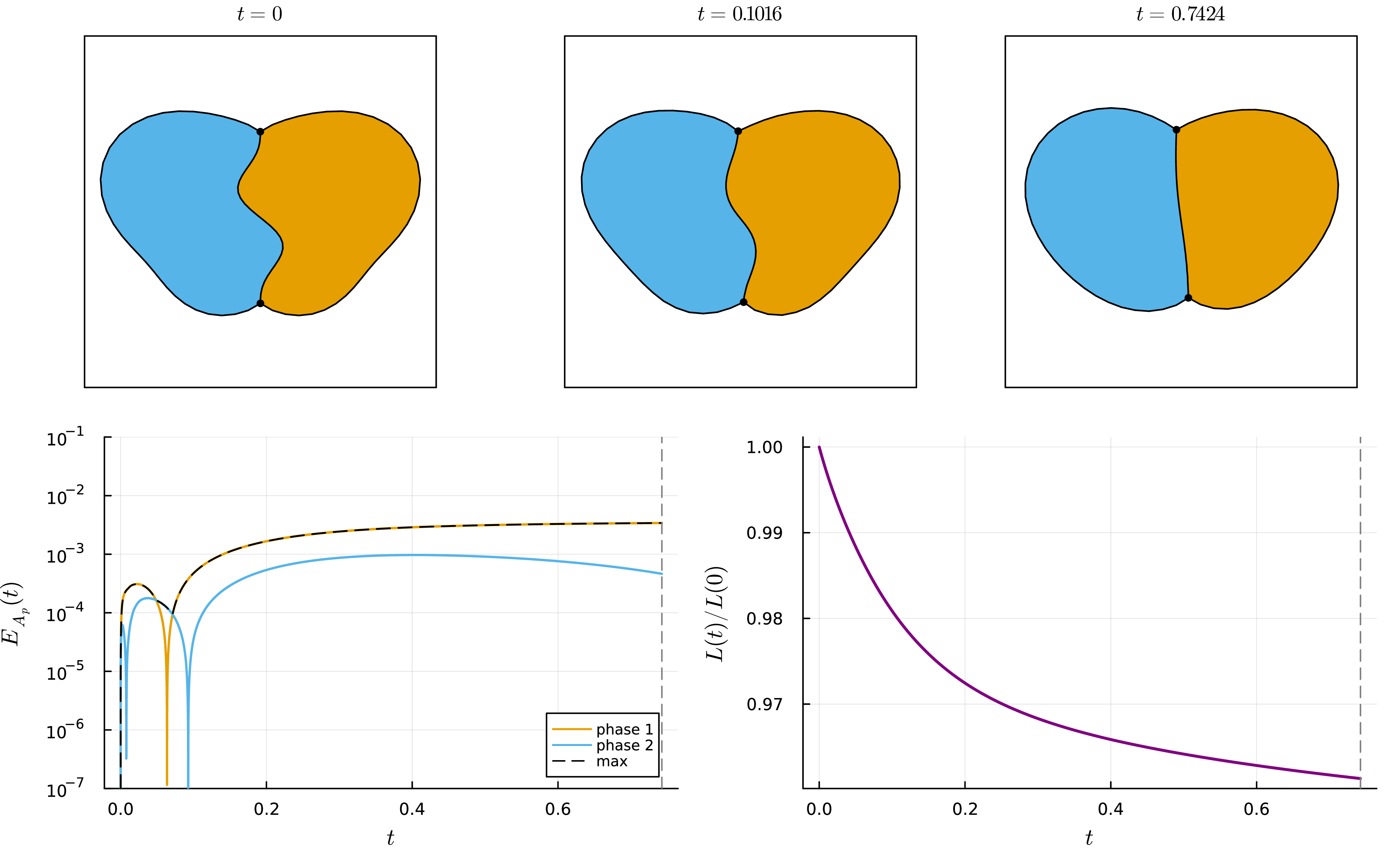
A four-phase network with four triple junctions probes robustness under a large geometric distortion: the prescribed topology and the four junctions are preserved at every step, the maximum phase-area drift is \(E_A=2.9\times10^{-3}\), and the network relaxes to a near-stationary configuration (Figure 9).
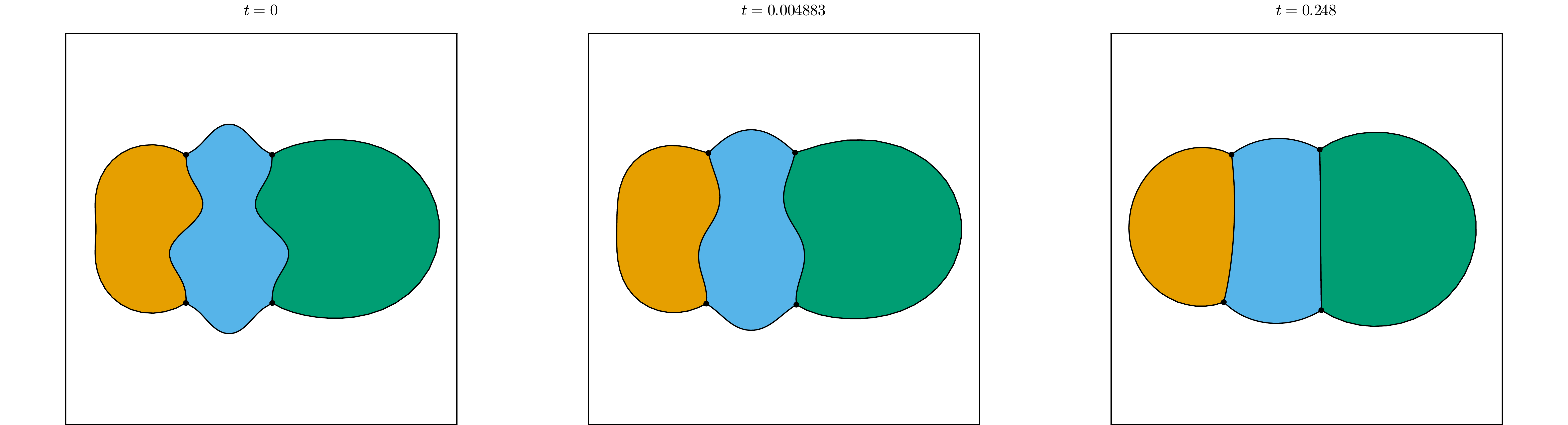
Finally, the scheme accommodates a network with both open and closed components: an open double-bubble coexisting with an isolated closed star-shaped curve, so the unbounded region has two boundary components. Under the flow the star rounds toward a circle (roundness \(r_{\min}/r_{\max}\colon 0.70\to0.98\)) while the open component relaxes without any topology change; the maximum area drift is \(E_A=7.1\times10^{-3}\) at this coarse resolution (Figure 10).
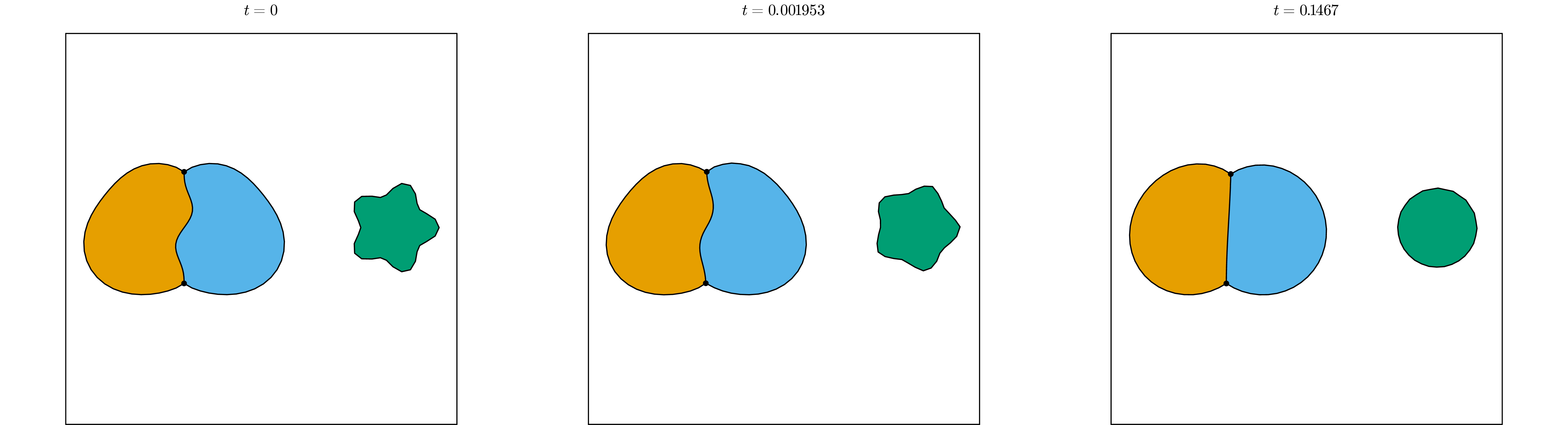
9.5 Unequal surface tensions and Young angles↩︎
The formulation of Section 2 admits unequal surface tensions \(\varsigma_{i}\); we validate the proposed scheme on a representative unequal-tension configuration against the Young angles. We take a triple-bubble lane of Section 9.4, whose bounded regions are identified by \(A\), \(B\), and \(C\), and raise the \(B\)–\(C\) interface tension to \(\varsigma_{BC} = 1.3\), leaving every other tension at \(1\). At a Gibbs–Thomson equilibrium, the three tension vectors at a junction balance, so the angle \(\theta_{ab}\) facing the curve of tension \(\varsigma_{c}\) satisfies the Young relation \[\label{eq:young-cos} \cos\theta_{ab} = \frac{\varsigma_{c}^2-\varsigma_{a}^2-\varsigma_{b}^2}{2\,\varsigma_{a}\varsigma_{b}},\tag{55}\] which is solvable precisely under the triangle inequalities of Remark 4. The two left junctions keep all tensions equal (Young angles \(120^\circ/120^\circ/120^\circ\)), while the two right junctions have tensions \((1,1.3,1)\) and hence the Young angles \(130.54^\circ/130.54^\circ/98.92^\circ\). The junction geometry is held at these per-junction Young angles by the geometric triple-junction correction of Section 6 (its \(120^\circ\) target generalized to the Young angles); the test is therefore not that the angles emerge unaided, but that the \(\varsigma_{}\)-weighted field solve stays consistent with them throughout the flow, conserving the phase areas and dissipating the weighted energy. We generalize the angle diagnostic 48 accordingly, replacing the target \(2\pi/3\) by the per-junction Young angle, and write \(E_{\angle}^{\mathrm{Young}}(t)\) for the resulting maximum deviation.
The run is reported at \(N=64\), with a companion \(N=32\) run, both summarized in Table 5. The measured junction angles track the Young targets to \(E_{\angle}^{\mathrm{Young}}<5\times10^{-5}\) degrees at every junction and both resolutions (Table 5), while the relative phase-area error stays at the same polygonal level as the equal-tension runs (\(E_A\le1.3\times10^{-4}\) at \(N=64\), \(1.6\times10^{-3}\) at \(N=32\)). The \(\varsigma_{}\)-weighted energy 49 decreases monotonically (after a brief initial adjustment while the discrete initial data settles), whereas the unweighted total length increases; the two are consistent because, once the tensions differ, it is the weighted length that the flow dissipates.
| TJ | tensions \((\varsigma_a,\varsigma_b,\varsigma_c)\) | Young angles [\(^\circ\)] | \(\max\Delta\theta\,[^\circ]\;(N{=}32)\) | \((N{=}64)\) |
|---|---|---|---|---|
| TL | \((1.0,\,1.0,\,1.0)\) | \(120.0/120.0/120.0\) | \(3.72\times10^{-5}\) | \(3.71\times10^{-5}\) |
| BL | \((1.0,\,1.0,\,1.0)\) | \(120.0/120.0/120.0\) | \(3.76\times10^{-5}\) | \(3.76\times10^{-5}\) |
| TR | \((1.0,\,1.3,\,1.0)\) | \(130.5/130.5/98.9\) | \(4.75\times10^{-5}\) | \(4.44\times10^{-5}\) |
| BR | \((1.0,\,1.3,\,1.0)\) | \(130.5/130.5/98.9\) | \(4.44\times10^{-5}\) | \(4.11\times10^{-5}\) |
9.6 Region disappearance↩︎
In the experiments so far, the network topology does not change. In this subsection, we treat the disappearance of a bounded region that is enclosed by a single closed curve and incident to no triple junction, once this curve has contracted below the resolution of the mesh; the extinction of a junction-bounded lobe or bubble is not treated, so the junction connectivity is never altered and no curve splicing or vertex surgery is involved. Because the area constraints pin the total area of each phase, an isolated bounded region cannot shrink on its own: disappearance requires the transfer of area between two regions of the same phase (intra-phase Ostwald ripening), which is possible because the region-to-phase map \(\mathscr R_p\) is non-injective. In this test, we confirm the multi-region phase introduced in Section 3.
9.6.0.1 Detection and removal.
A closed curve \(\Gamma^h_{i}\) is flagged for removal once the area it encloses falls below a prescribed threshold, \[\label{eq:disappear-delta} A_i < \delta.\tag{56}\] For a refinement sequence, a resolution-tied choice is \(\delta_N=c_\delta h_N^2\), where \(h_N:=\max_j|\sigma_{i,j}|\) is the maximum edge length of the candidate curve at the removal step and \(c_\delta>0\) is held fixed. With this choice, the area removed at an event is bounded by \(c_\delta h_N^2\) and therefore vanishes as \(h_N\to0\). At that step, the curve is deleted, and the incidence data of Section 3 are updated: the vanished region is removed from \(\mathscr C_r\) and \(\mathscr R_p\), the two regions formerly separated by \(\Gamma^h_{i}\) are merged, and the conserved-area target of the affected phase is reset to its new polygonal value. The charge-point layout and the constraint matrix \(C\) are rebuilt for the reduced configuration, and the evolution continues. The removal is an opt-in module of the solver, checked against the unchanged fixed-topology path by regression tests. Between events, every phase area is conserved at the velocity level (Proposition 4); the removal step changes the affected phase total by exactly the residual \(A_i<\delta\), an identity that vanishes as \(\delta\to0\) along such a refinement sequence (Remark 18) and is reported as a single step in the per-phase area history.
We first let a region disappear from a phase whose area is unconstrained, by running the exact three-circle solution of Section 9.1 through to its natural end. Under 52 the conserved inner-annulus squared-radius gap \(D_2=R_2^2-R_1^2\) (whose area is \(\pi D_2\)) forces \(R_1\to0\) as \(R_2\to\sqrt{D_2}\): the inner disk, a bounded component of the unbounded phase \(3\), collapses and vanishes at the finite time \[\label{eq:disappear-tstar} t^* = \int_{\sqrt{D_2}}^{R_2(0)} \frac{\mathrm{d}u}{F(u)} = 1.6189 \quad\text{(to machine precision)},\tag{57}\] with \(F\) as in 53 ; the integrand is integrable at the endpoint (\(1/F\sim R_1\log(1/R_1)\to0\)), and after the event the exact solution is the stationary pair of concentric circles bounding the two conserved annuli. Because the vanishing region belongs to the unbounded phase, its removal leaves the two conserved annulus areas unchanged.
We integrate the discrete flow with the detector in report-only mode (no removal is triggered) at \(N\in\{32,48,64\}\) and \(\Delta t = cN^{-2}\), recording the discrete event time \(t_{ev}(\delta)\), the first step at which the discrete disk area falls below \(\delta\). In this calibration, each listed value of \(\delta\) is held fixed across the three resolutions; the test therefore isolates convergence of the discrete threshold-crossing time to the corresponding exact time \(t^*(\delta)\), not convergence under the coupled choice \(\delta_N=c_\delta h_N^2\). Table 6 compares \(t_{ev}(\delta)\) with \(t^*(\delta)\): the error at \(\delta=0.02\) decreases as \(0.220,\,0.164,\,0.127\) for \(N=32,48,64\), an observed order \(p\approx0.79\) toward the exact threshold-crossing time \(t^*(0.02)\). The error is dominated by the spatial resolution: at fixed \(N=32\), varying \(c\) over \(\{0.5,0.2,0.1,0.05\}\) moves \(t_{ev}(0.02)\) by less than \(10^{-3}\). Across the event the two conserved annulus areas stay flat: their drift is the higher-order polygonal amount, of order \(10^{-5}\)–\(10^{-4}\) before the terminal collapse layer (decreasing with \(N\)) and rising to \(\sim10^{-3}\) within that layer at the coarsest \(N=32\) (Figure 11).
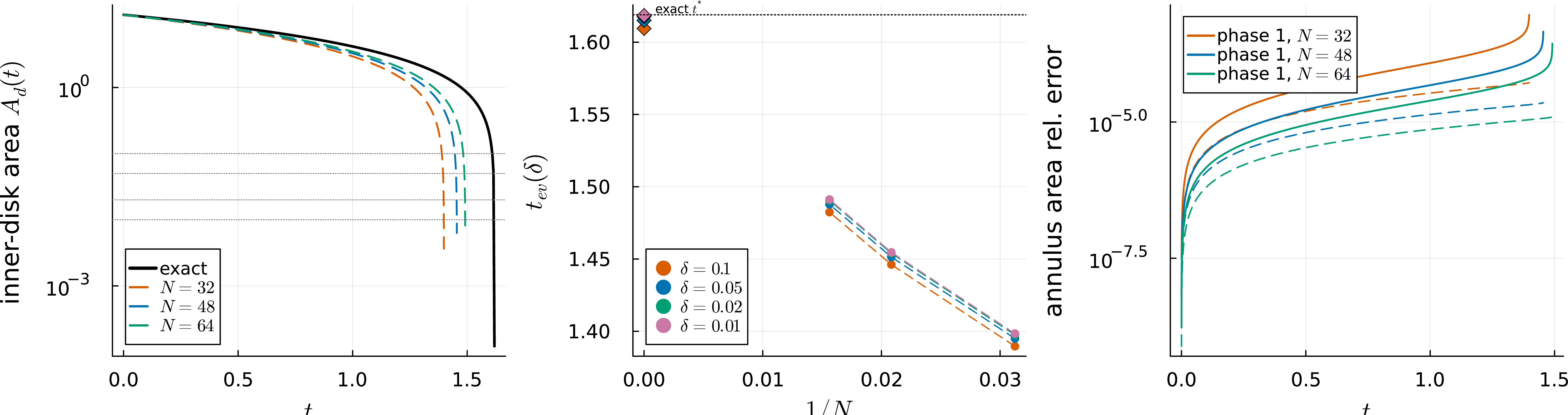
| \(N\) | \(\Delta t\) | \(t_{ev}(0.10)\) | \(t_{ev}(0.05)\) | \(t_{ev}(0.02)\) | \(t_{ev}(0.01)\) | \(|t_{ev}(0.02)-t^*(0.02)|\) |
|---|---|---|---|---|---|---|
| 32 | 4.88e-04 | 1.3896 | 1.3950 | 1.3975 | 1.3984 | 0.2203 |
| 48 | 2.17e-04 | 1.4462 | 1.4514 | 1.4540 | 1.4546 | 0.1638 |
| 64 | 1.22e-04 | 1.4824 | 1.4878 | 1.4905 | 1.4912 | 0.1273 |
| exact \(t^*(0.02)=1.6178\), \(t^*=1.6189\) (machine precision); observed order \(p\approx0.79\). | ||||||
The dual case, in which the vanishing regions belong to constrained phases, corresponds to the coarsening scenario of the introduction: two dispersed phases, each split into three disks of distinct radii, embedded in the unbounded matrix phase (six closed curves, no triple junctions). Figure 12 shows the flow at \(N=48\) with the detector active. The four satellite disks vanish in order of increasing size, alternating between the two phases, at \(t=0.081\), \(0.153\), \(0.240\), and \(0.408\); after the last event the two surviving disks relax to the near-stationary state of 51 at \(t\approx0.96\), one round disk per phase (roundness \(0.995\) and \(0.996\)). Between events the two constrained phase totals are flat up to a polygonal drift below \(7\times10^{-5}\); at each event the affected phase total drops by exactly the removed residual, \(0.47\%\)–\(0.53\%\) of the phase area; the accounting identity of the removal step holds to rounding (\(\le4.5\times10^{-16}\)). Each step of the staircase in the middle bottom panel of Figure 12 thus equals exactly the sub-resolution residual (\(<\delta\)) of a vanished region, an amount bounded by the prescribed removal threshold 56 . The run reproduces the three properties stated in the introduction: the large regions grow at the expense of the small, the total interfacial length decreases (\(L(T)/L(0)=0.62\)), and the area of each phase is conserved up to the four disclosed residuals.
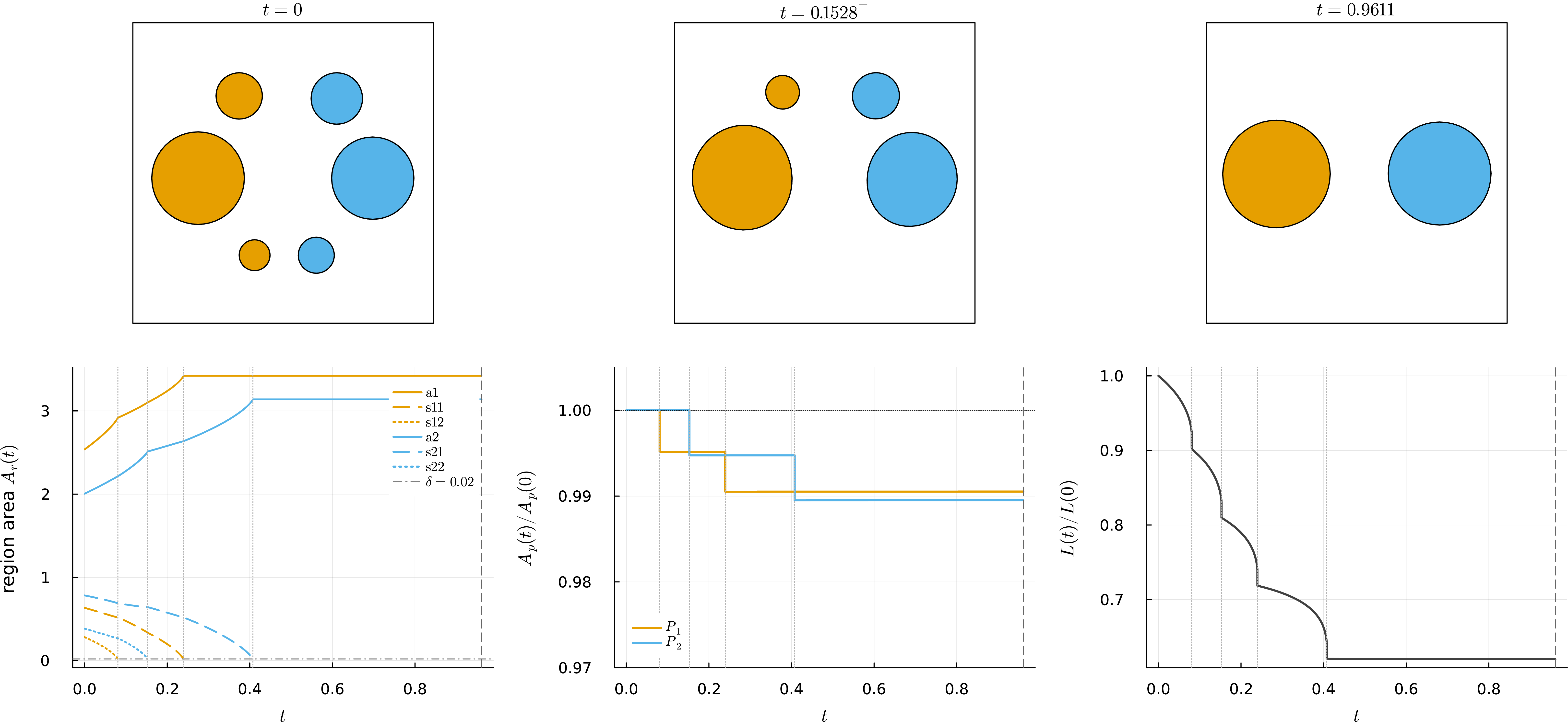
Remark 19. Julin, Morini, Ponsiglione, and Spadaro [49] have shown that any initial data \(E_0\subset\mathbb{R}^{2}\) having perimeter less than \(2\) asymptotically converges to a union of disks whose areas sum up to the initial volume \(|E_0|\) in the two-phase case under a periodic boundary condition. We observe a similar phenomenon in Figure 12 for the three-phase case.
9.7 Half space↩︎
We now validate the half-space scheme of Section 7, in which open curves may end on the Neumann wall as mobile contacts. All runs use the constrained velocity solve of Section 7.3, the on-manifold Heun update of Section 7.4, and the edge-rate redistribution constant \(\beta_0=10\); the update keeps the \(90^\circ\) wall contacts and the \(120^\circ\) junctions exact by construction, the discrete area-rate rows are met to solver precision, and the polygonal region areas drift by the small amounts quoted. In the half-space figures the thick black line is the Neumann wall \(\mathcal{W}\), mobile wall contacts are white markers, and interior triple junctions black dots; the bottom panels report the same area-error and energy diagnostics as in Section 9.4.
We begin with a three-phase \(M\)-branch: three open curves meeting at one interior triple junction with three mobile wall contacts, started from a strongly asymmetric, unbalanced state (\(A_2\!:\!A_1 = 7\!:\!10\)). At a Gibbs–Thomson equilibrium every arc has constant curvature, so the expected shape class is an asymmetric circular-arc double arch. Under the flow the network relaxes toward this class: the interfaces approach circular arcs, the contact and junction angles are held exactly by the endpoint-chart update, the prescribed areas are preserved, the final Gibbs–Thomson residual falls below the \(0.05\) threshold, and the interfacial energy decreases to a plateau while the imposed size imbalance persists (Table 7, Figure 13).
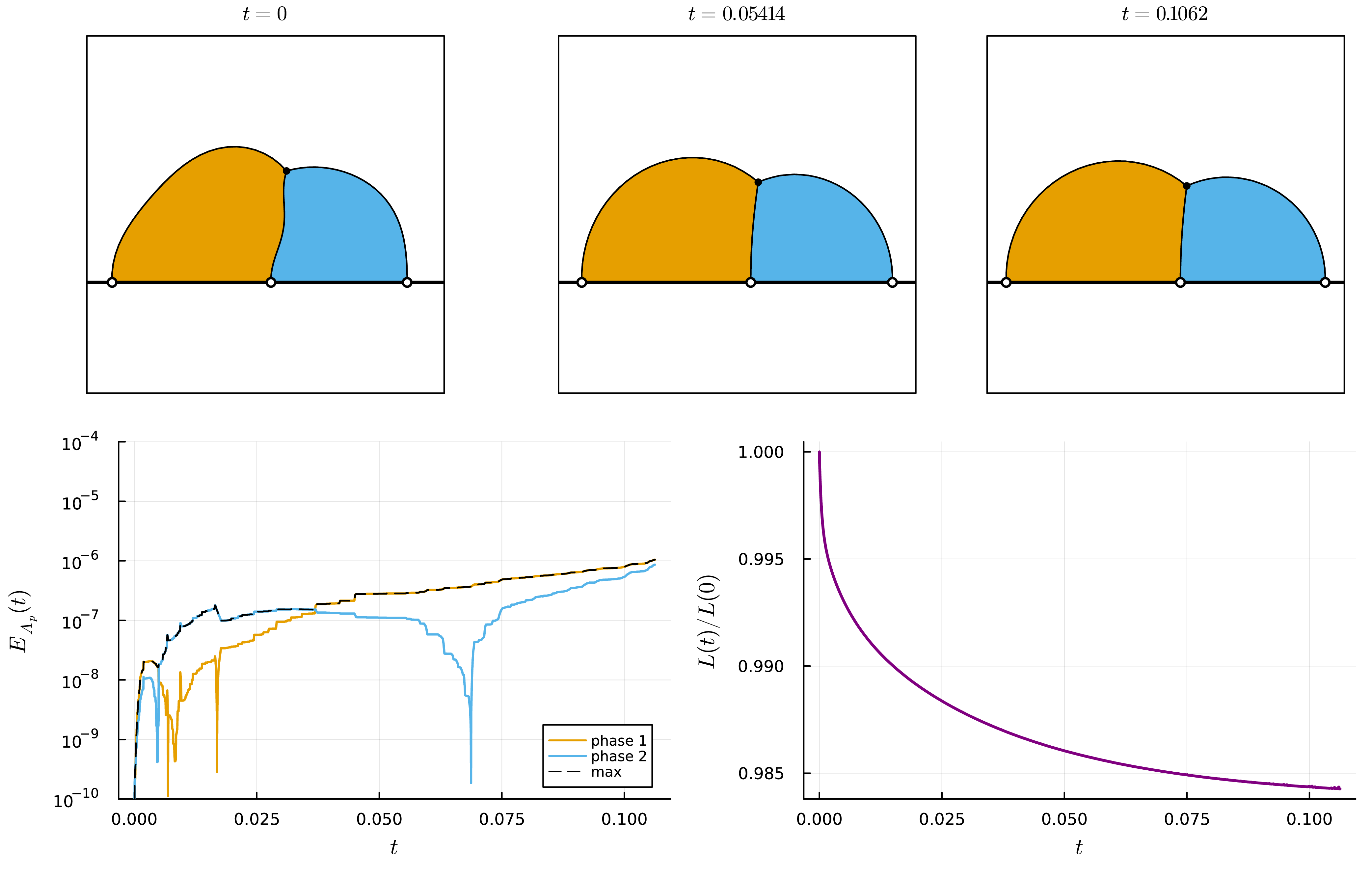
| quantity | value |
|---|---|
| circle-fit residual per unit length (\(t=0\to T\)) | \(3.8\times10^{-3}\) \(\to\) \(1.0\times10^{-3}\) |
| max wall-contact angle deviation from \(90^\circ\) | \(0\) (machine) |
| max triple-junction angle deviation from \(120^\circ\) | \(1.4\times10^{-11}\) deg |
| max phase-area drift \(E_A\) | \(1.0\times10^{-6}\) |
| final Gibbs–Thomson residual | 0.019 |
| interfacial energy \(L(T)/L(0)\) | 0.984 |
To exercise many independently mobile contacts we scale the configuration up. Figure 14 shows a strongly perturbed four-phase / three-junction network with three mobile wall contacts, relaxed toward a near-stationary asymmetric double arch (the maximum normal speed decays to well under \(1\%\) of its peak and the length approaches a plateau): the contacts remain ordered and meet the wall orthogonally, the three triple junctions are preserved, and the bounded areas are conserved to solver precision.
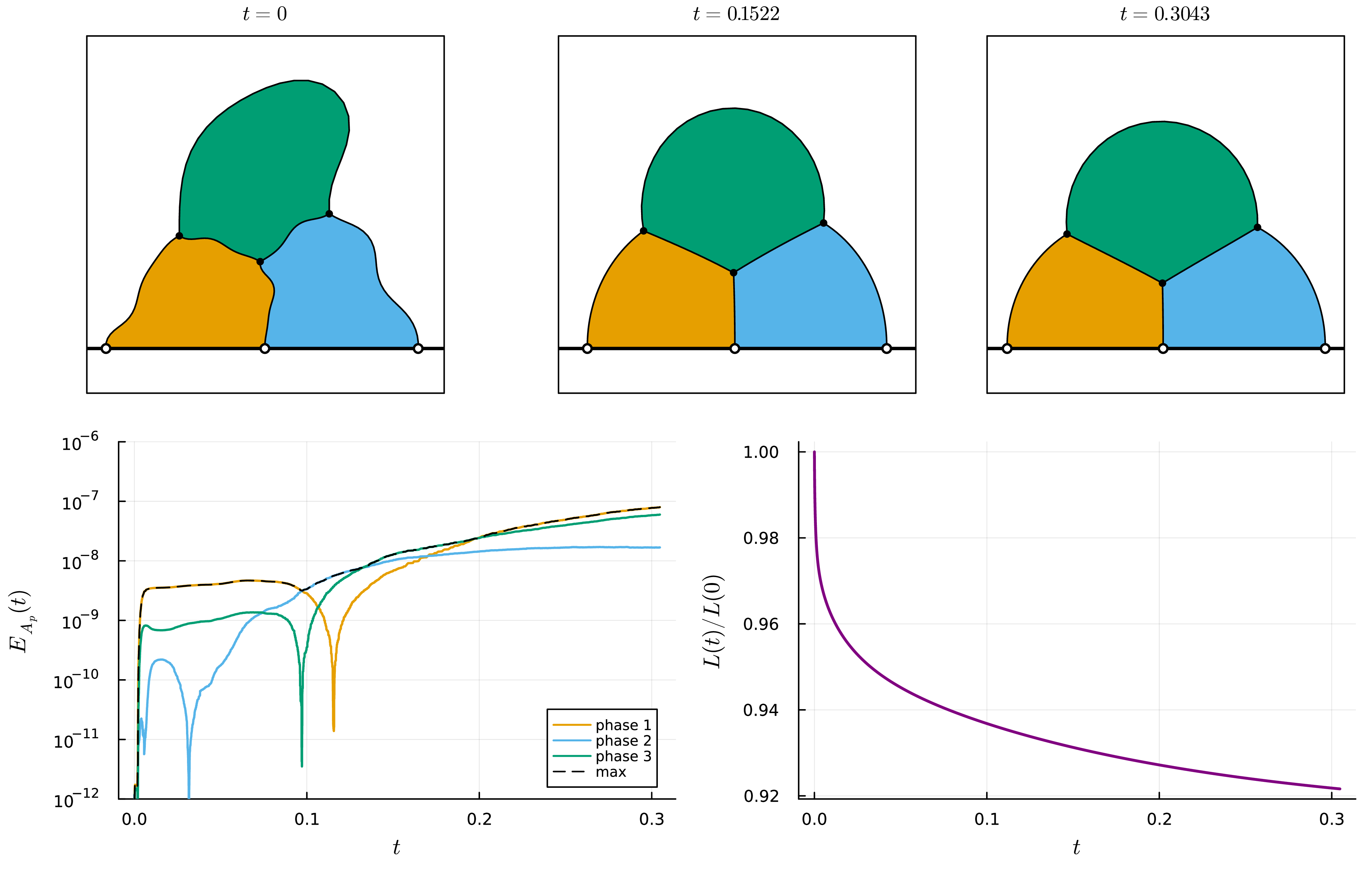
10 Conclusion↩︎
In this paper, we have developed a bulk mesh-free solver for the multi-phase Mullins–Sekerka flow based on the CSM, which is a variant of the MFS, in the planar case together with the half-plane case. Representing each chemical potential by a combination of fundamental solutions to the Laplace equation centered at off-interface charge points has removed the need for a bulk mesh and the singular integrals, leaving only the interfacial conditions to impose. The discretization preserves the discrete area constraints exactly by projecting the reconstructed velocity onto their null space. Between topological events, every bounded phase area is conserved to machine precision at the velocity level; the only topological event treated here is the disappearance of a region enclosed by a single closed curve and incident to no junction. The pure Neumann boundary condition is imposed exactly by image charges, and mobile contacts are kept orthogonal to the boundary, and triple junctions remain in balance according to the Herring–Young law. The accuracy of the proposed scheme has been validated against an exact three-concentric-circle solution to the underlying model; its outcome has been compared with the parametric finite element approach, and, for the case where \(N = 128\), the proposed scheme has yielded a comparable interface error without a bulk mesh.
The structural result proved here is conditional on the non-degeneracy assumption 46 and concerns exact phase-area conservation at the reconstructed-velocity level. For curve networks with moving triple junctions and wall contacts, for which no exact benchmark is available, the curvature correction and the half-space constrained update have instead been assessed through refinement diagnostics, constraint residuals, area errors, and energy dissipation. A convergence and stability analysis of discretization of triple junctions and half-space curve networks remains an open problem.
References↩︎
Université Claude Bernard Lyon 1, CNRS, Centrale Lyon, INSA Lyon, Université Jean Monnet, ICJ UMR5208, 69622 Villeurbanne, France. email:eto@math.univ-lyon1.fr↩︎