RFMSR: Residual Flow Matching for Image Super-Resolution
July 14, 2026
Abstract
Image super-resolution (ISR) has witnessed remarkable progress with diffusion models and flow matching. The dominant text-to-image (T2I) based approaches leverage large-scale foundation models as generative priors, achieving impressive perceptual quality but at the cost of massive model sizes and prohibitive training expenses. Recent flow-matching-based vision-only approaches have made significant strides; however, they adopt standard flow formulations that transport from a pure Gaussian prior to the data distribution, discarding the rich structural information already present in the low-quality (LQ) input. Furthermore, existing single-step acceleration techniques often forfeit the model’s multi-step inference capability. In this paper, we propose Residual Flow Matching for Image Super-Resolution (RFMSR), a vision-only framework that centers the source distribution at the LQ latent, reducing transport distance and preserving structural priors throughout the flow trajectory. We further introduce a two-phase training strategy: Phase I pretrains the velocity field via conditional flow matching, while Phase II applies end-to-end supervision to the single-step prediction while retaining the velocity loss across all timesteps, achieving high-quality single-step generation without sacrificing multi-step refinement. Extensive experiments demonstrate that RFMSR achieves comparable or even superior perceptual quality compared to state-of-the-art (SOTA) methods. The source code is available at https://github.com/Faze-Hsw/RFMSR.
1 Introduction↩︎
Image super-resolution (ISR) aims to reconstruct a high-quality (HQ) image from its low-quality (LQ) counterpart. While early deep learning methods [1]–[4] achieved impressive pixel-level accuracy, they often produce over-smoothed results that lack high-frequency details. To improve perceptual quality, GAN-based approaches [5]–[8] employ adversarial training to generate realistic textures. However, GAN training can be unstable and may introduce unpleasant artifacts. Recent advances in generative modeling, particularly diffusion models [9]–[11] and flow matching [12], [13], have enabled more stable and perceptually rich image restoration by learning to sample from the natural image distribution.
A dominant trend in generative ISR leverages large-scale text-to-image (T2I) foundation models such as Stable Diffusion [14] as strong image priors. Methods like StableSR [15], DiffBIR [16], and SeeSR [17] fine-tune these pre-trained models with degradation-aware conditioning and achieve impressive perceptual quality. To reduce the high inference cost of multi-step diffusion, subsequent works pursue single-step generation via knowledge distillation [18], [19] or consistency training [20]. However, these T2I-based approaches come with notable drawbacks: they inherit the massive parameter sizes of foundation models, incur substantial training costs, and are inherently constrained by the quality and biases of the pre-trained teacher. Furthermore, these methods rely on external text prompts as conditional semantics, which often introduce artifacts and hallucinated details inconsistent with the LQ input.
In parallel, vision-only approaches bypass T2I pretraining entirely. SR3 [21] first introduced diffusion models to image super-resolution by iteratively refining noisy inputs through a learned denoising process. ResShift [22] advanced this direction by constructing a shorter Markov chain that shifts the residual between LQ and HQ images. SinSR [23] distilled ResShift into a single-step model. These earlier vision-only methods, however, are constrained by limited model capacity and the absence of large-scale pretraining, leaving their perceptual quality behind T2I-based approaches. VOSR [24] addressed this gap by combining flow matching with a large model backbone [25] and DINOv2 [26] semantic conditioning, and training on extensive data, demonstrating that vision-only models can match T2I-based methods. Despite this breakthrough, VOSR still inherits a key limitation of standard flow matching: it adopts a pure Gaussian distribution as the source prior for image generation, overlooking the structural information already present in the LQ input.
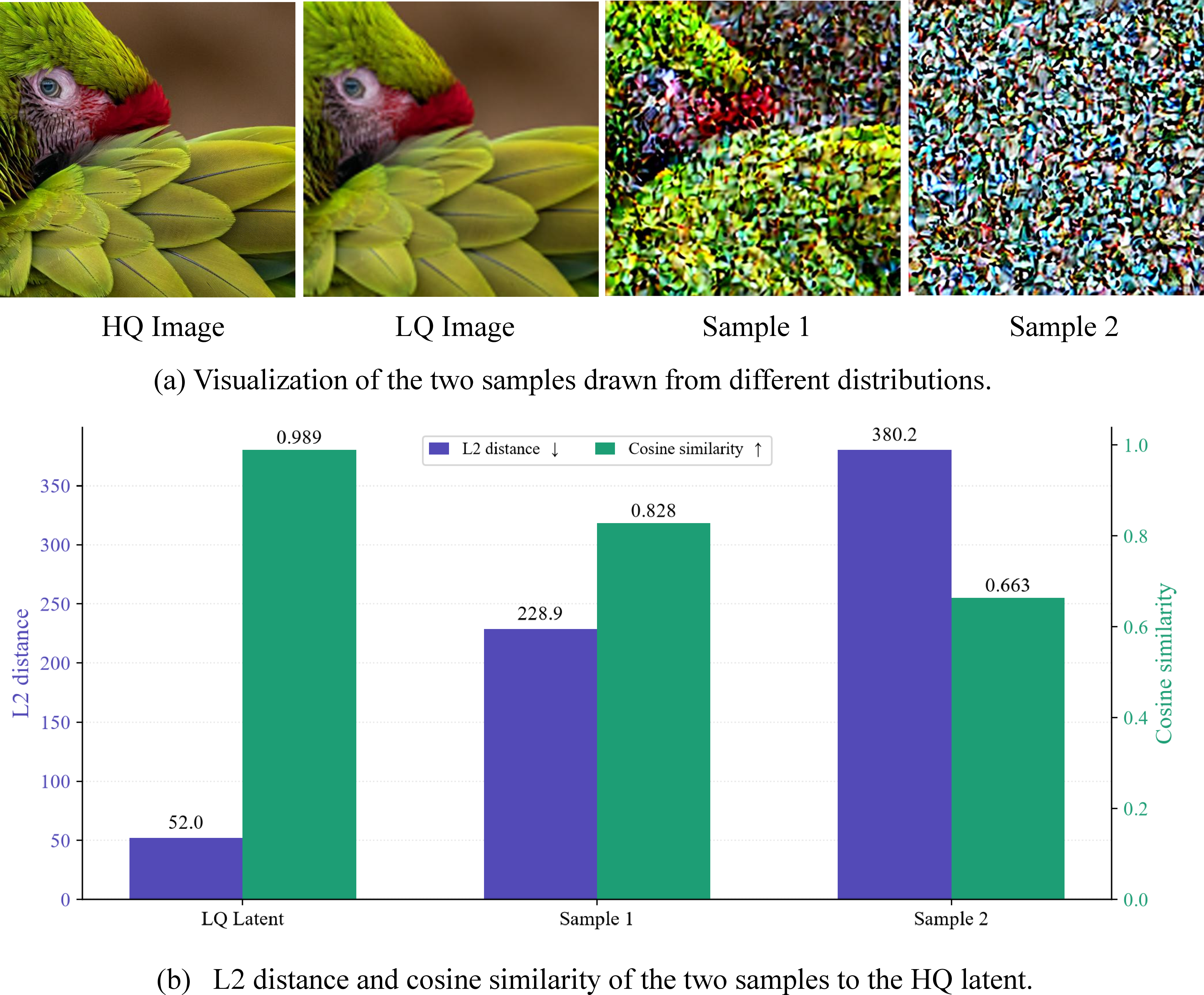
In this paper, we propose Residual Flow Matching for Image Super-Resolution (RFMSR), a vision-only framework that reformulates flow matching for the ISR task. Inspired by the residual-shifting strategy of ResShift [22] for diffusion-based ISR, our key insight is that the LQ image provides substantial prior knowledge about the target HQ image, and the flow should leverage this information rather than starting from pure noise. Specifically, we define the source distribution as a Gaussian centered at the LQ latent \(y_0\) with variance \(\sigma^2\), , \(p_1 = \mathcal{N}(y_0, \sigma^2 I)\). As shown in 1, this residual flow formulation reduces the transport distance and preserves structural priors throughout the trajectory, enabling more efficient and faithful reconstruction.
Beyond architectural design, real-world deployment typically demands single-step generation for efficiency. Common one-step distillation approaches, such as the variational score distillation [27] employed in OSEDiff [18] or consistency training [20], permanently forfeit the model’s multi-step inference capability, precluding further improvement in perceptual quality through additional sampling steps. To address this, we propose a training strategy that directly applies end-to-end supervision to the single-step prediction quality, while concurrently retaining the standard velocity loss of flow matching across all timesteps. This design endows the model with flexible inference ranging from a single forward pass to multi-step refinement.
Our contributions are summarized as follows:
We propose Residual Flow Matching for ISR, which centers the source distribution at the LQ latent to reduce transport distance and preserve structural priors, outperforming standard rectified flow with the same architecture and training budget.
We design a two-phase training strategy that achieves high-quality single-step generation while fully retaining multi-step inference capability, combining the flexibility of flow matching with the efficiency of end-to-end supervision.
Extensive experiments validate the effectiveness of the residual flow matching formulation over standard flow matching, demonstrate that the proposed training strategy preserves multi-step flexibility while achieving strong single-step performance, and show that the vision-only framework can surpass T2I-based methods across multiple benchmarks without relying on foundation model priors.
2 Related Work↩︎
Diffusion models [9], [10] and flow matching [12], [13] have become dominant generative frameworks for ISR, operating in the latent space of a pre-trained VAE [28]. Existing methods fall into two broad categories: T2I-based and vision-only.
T2I-based methods leverage generative priors from large-scale pre-trained text-to-image foundation models. StableSR [15] fine-tunes Stable Diffusion with degradation-aware conditioning and a feature wrapping module, while DiffBIR [16] separates restoration into structure recovery and diffusion-based detail refinement. SeeSR [17] incorporates semantic-aware prompts, and InvSR [19] enables flexible-step inference through diffusion inversion. PASD [29] enhances pixel-level perception via cross-attention, while SUPIR [30] scales up both model and data with restoration-guided sampling. Despite producing visually compelling results, these methods suffer from two key drawbacks: they inherit the massive computational footprint of foundation models, and their reliance on text prompts risks generating hallucinated textures misaligned with the original LQ scene.
Vision-only methods avoid T2I pretraining and train diffusion or flow-based models from scratch. SR3 [21] pioneered diffusion-driven ISR, and ResShift [22] improved efficiency by shifting the residual between LQ and HQ images over a shorter Markov chain. SinSR [23] further distilled ResShift into a single-step model. More recently, VOSR [24] integrated flow matching with DINOv2 [26] semantic features and partial conditioning, achieving performance competitive with T2I-based approaches. However, VOSR retains the standard flow formulation—transporting from pure Gaussian noise to the HQ distribution—which discards the structural priors embedded in the LQ input. Our RFMSR resolves this by centering the source distribution at the LQ latent, preserving structural information throughout the flow trajectory.
Single-step acceleration. The multi-step sampling process incurs high inference latency, spurring research on single-step ISR generation. In the T2I-based setting, OSEDiff [18] applies variational score distillation to compress a pre-trained diffusion model, TSD-SR [31] introduces target score distillation with real HQ references, and YONOS-SR [32] progressively transfers knowledge across upscaling factors. FluxSR [33] and FlowSR [34] extend distillation to flow-based backbones. In the vision-only domain, SinSR [23] distills ResShift into a single-step student. Consistency models [20] offer an alternative by learning self-consistent ODE mappings without a teacher. A critical limitation shared by both paradigms is that they permanently sacrifice multi-step capability—once compressed, the model cannot be further refined.
Our two-phase training strategy departs from these paradigms. Instead of distilling a teacher or enforcing self-consistency, we supervise the one-step prediction with end-to-end reconstruction losses while retaining the standard flow matching velocity loss across all timesteps. This preserves the model’s native ability to perform inference with arbitrary step counts, from fast single-step generation to quality-enhanced multi-step refinement.
3 Method↩︎
![Figure 2: Overview of RFMSR. We uniformly sample 15 points in [0,1] and display a subset of the intermediate states. Forward (top): the HQ latent x_0 is progressively transformed toward a Gaussian distribution centered at the LQ latent y_0. Reverse (bottom): a latent sampled near y_0 is progressively refined into the final ISR result.](/article/2607.12753/figs/residual_flow_overview.png "fig:")
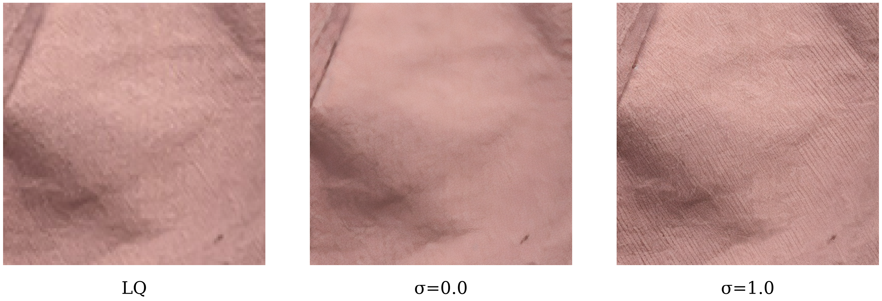
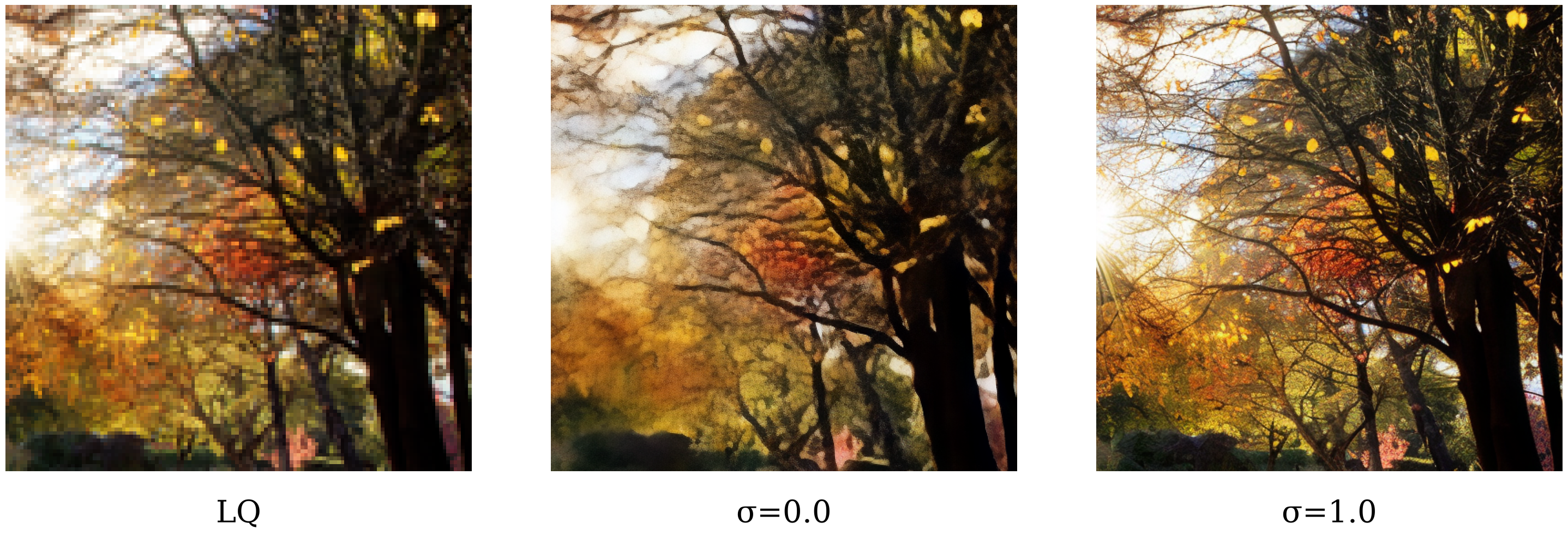
Figure 3: Visual effect of the noise level \(\sigma\). At \(\sigma=0.0\), the model collapses to a deterministic regression with over-smoothed outputs; increasing \(\sigma\) to \(1.0\) restores perceptually richer details. (Zoom in for best view.).
3.1 Preliminaries↩︎
We begin by briefly reviewing the flow matching framework [12], [13]. Let \(p_1\) denote a simple prior distribution (, a Gaussian distribution) and \(p_0\) the target data distribution. A flow \(\phi_t\) governed by the ODE \[\frac{dx_t}{dt} = v_\theta(x_t, t), \quad t \in [0, 1],\] transports samples from \(p_1\) to \(p_0\), where \(v_\theta\) is a velocity field parameterized by a neural network. Given \(x_1 \sim p_1\), a data point \(x_0 \sim p_0\) can be generated by integrating \(v_\theta\) from \(t = 1\) to \(t = 0\). This defines a probabilistic path \(p_t\) from \(p_0\) to \(p_1\), where \(p_t\) denotes the marginal distribution of \(x_t\) at time \(t \in [0, 1]\). Training \(v_\theta\) via maximum likelihood in the continuous normalizing flow framework is prohibitively expensive, as the marginal probability path \(p_t(x)\) is intractable. Conditional Flow Matching (CFM) [12] circumvents this by conditioning on both endpoints. Specifically, one defines a conditional probability path \(p_t(x \mid x_1, x_0)\) and the corresponding conditional velocity field \(v_t(x \mid x_1, x_0)\), then minimizes \[\mathcal{L}_{\text{CFM}}(\theta) = \mathbb{E}_{t,\, x_1 \sim p_1,\, x_0 \sim p_0}\Big[ \big\| v_\theta(x_t, t) - v_t(x_t \mid x_1, x_0) \big\|^2 \Big],\] where \(t \sim \mathcal{U}[0, 1]\). A canonical choice is the straight path proposed by Rectified Flow [13], which yields \[x_t = (1 - t)\, x_0 + t\, x_1, \qquad v_t(x_t \mid x_1, x_0) = x_1 - x_0.\] During inference, one draws \(x_1 \sim p_1\) and solves the ODE backward from \(t = 1\) to \(t = 0\) using a numerical integrator (, Euler method).
3.2 Residual Flow Matching for ISR↩︎
The standard flow matching formulation assumes \(p_1\) to be a standard Gaussian \(\mathcal{N}(0, I)\), which is a natural choice for T2I generation tasks [35], [36] where the target distribution is conditioned on a text prompt rather than an input image. For ISR tasks, however, the LQ image provides substantial structural information about the target HQ image. Starting from pure noise discards this information and forces the model to traverse an unnecessarily long probability path.
Following [22], we propose Residual Flow Matching for ISR (RFMSR), which constructs the source distribution centered around the LQ image. Let \(x_0, y_0\) denote the HQ and LQ images encoded by a pre-trained VAE encoder (SD 2.1 [37] in our implementation). We define the source distribution as \[p_1 = \mathcal{N}\big(y_0,\, \sigma^2 I\big),\] where \(\sigma\) is a hyperparameter that controls the initial noise strength. The conditional flow path from source (\(t = 1\)) to target (\(t = 0\)) is a linear interpolation augmented with a time-dependent noise injection: \[x_t = x_0 + t \cdot \big(y_0 - x_0\big) + t \cdot \sigma \cdot \varepsilon, \quad \varepsilon \sim \mathcal{N}(0, I). \label{eq:rfmsr95path}\tag{1}\] Notably, at \(t = 0\), \(x_t\) converges to the clean HQ latent \(x_0\), while at \(t = 1\), \(x_t\) follows a Gaussian distribution centered at the LQ latent \(y_0\). The conditional velocity field \(v_t\) follows directly from differentiation: \[v_t(x_t \mid x_1, x_0) = \frac{d x_t}{d t} = x_1 - x_0, \quad x_1 \sim \mathcal{N}(y_0, \sigma^2 I).\] The training loss follows directly from the CFM framework: \[\mathcal{L}(\theta) = \mathbb{E}_{t,\, x_0 \sim p_0,\, x_1 \sim \mathcal{N}(y_0, \sigma^2 I)}\Big[ \big\| v_\theta(x_t, t, c) - (x_1 - x_0) \big\|^2 \Big]. \label{eq:rfm95loss}\tag{2}\] where \(c\) denotes the LQ conditioning information.
An illustrative trajectory of the proposed residual flow is shown in 2. Notably, the initial state sampled from \(p_1\) already retains the structural information of the LQ image, which significantly reduces the difficulty of the restoration process compared to starting from pure noise.
3.3 Why Noise Matters↩︎
A natural simplification of 1 would be to remove the noise term entirely, , \(x_t = x_0 + t\,(y_0 - x_0)\). This deterministic path corresponds to \(v_t = y_0 -
x_0\), reducing the learning objective to a plain \(\mathcal{L}_2\) regression of the residual. While conceptually simple, this design suffers from a fundamental limitation.
Perceptual degradation. ISR is an inherently ill-posed, one-to-many inverse problem: a single LQ image admits multiple plausible HQ reconstructions that differ in fine-grained textures and high-frequency details. Under the deterministic
path, the \(\mathcal{L}_2\) objective forces the model to predict the conditional expectation \(\mathbb{E}[x_0 \mid y_0]\), which is the pixel-wise mean over all plausible HQ
reconstructions. This leads to over-smoothed outputs that lack high-frequency details. As shown in 3, the deterministic variant (\(\sigma=0.0\)) produces noticeably blurrier results
than RFMSR (\(\sigma=1.0\)), particularly in textured regions. Quantitative results reported in the Appendix further confirm this: while the deterministic model achieves comparable PSNR and SSIM [38], it suffers a significant degradation in perceptual metrics.
3.4 Single-Step Generation via Two-Phase Training↩︎
While flow matching models naturally support multi-step inference with arbitrary step counts, real-world deployment often demands single-step generation for low latency. Recent works accelerate flow-based or diffusion-based ISR through knowledge
distillation [18], [31]–[34] from large-scale pre-trained text-to-image (T2I) models to produce a one-step student model. However, these approaches typically sacrifice the model’s native multi-step capability: the distilled student operates
exclusively in the one-step regime and no longer benefits from progressive refinement, and the performance of distilled models is inherently bounded by that of the teacher model. Moreover, distilling large-scale T2I models incurs substantial computational
cost, and fine-tuning these massive models remains expensive. In contrast, our RFMSR is a purely vision-based model with a lightweight design, which enables a more flexible training paradigm. We propose a two-phase training strategy that endows the model
with high-quality single-step generation while fully preserving its multi-step inference capability.
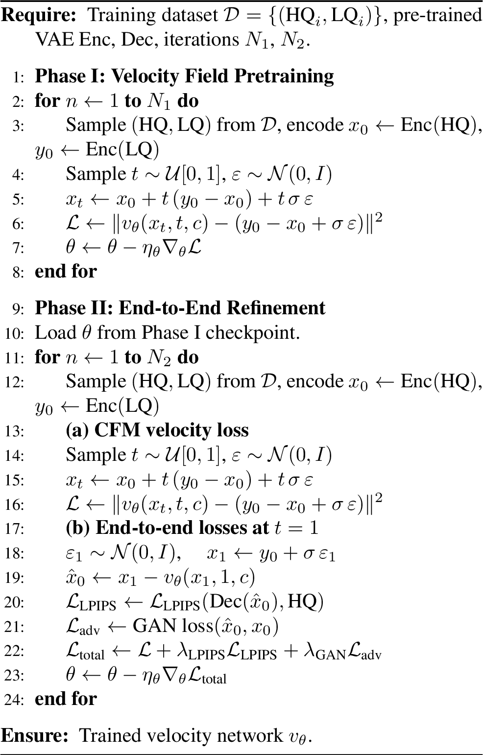
Phase I: Velocity Field Pretraining. In the first phase, we train the model using only the CFM objective defined in 2 . The model learns the conditional velocity field \(v_\theta(x_t, t, c)\) across all \(t \in [0, 1]\), establishing a smooth transport from the source distribution \(\mathcal{N}(y_0, \sigma^2 I)\) to the target HQ
latent distribution. This phase produces a general-purpose flow model capable of multi-step Euler integration.
Phase II: End-to-End Refinement. Starting from the Phase I checkpoint, we introduce two end-to-end losses operating on the one-step prediction \(\hat{x}_0 = x_1 - v_\theta(x_1, 1, c)\): an LPIPS perceptual
loss [39] and a PatchGAN [40] with hinge loss [41]. Crucially, we retain the CFM velocity loss \(\mathcal{L}(\theta)\) from Phase I. The full Phase II objective is: \[\mathcal{L}_{\text{Phase II}} = \mathcal{L}(\theta) + \lambda_{\text{LPIPS}}\, \mathcal{L}_{\text{LPIPS}}(\hat{x}_0,\, x_0) +
\lambda_{\text{GAN}}\, \mathcal{L}_{\text{adv}}(\hat{x}_0,\, x_0),\] where the CFM term continues to sample \(t \sim \mathcal{U}[0, 1]\). The complete two-phase procedure is summarized in Algorithm 4.
4 Experiments↩︎
| Dataset | Type | Method | PSNR\(\uparrow\) | SSIM\(\uparrow\) | LPIPS\(\downarrow\) | DISTS\(\downarrow\) | NIQE\(\downarrow\) | MUSIQ\(\uparrow\) | MANIQA\(\uparrow\) | CLIPIQA\(\uparrow\) | FID\(\downarrow\) |
|---|---|---|---|---|---|---|---|---|---|---|---|
| LSDIR | Multi-Steps | SeeSR-50 | 20.27 | 0.5049 | 0.2538 | 0.1528 | 4.1000 | 72.3832 | 0.5594 | 0.7142 | 50.92 |
| VOSR-25 | 20.05 | 0.4972 | 0.2348 | 0.1455 | 3.8119 | 71.5792 | 0.4729 | 0.6184 | 45.22 | ||
| ResShift-4 | 20.64 | 0.5277 | 0.2251 | 0.1422 | 5.3839 | 67.3639 | 0.4360 | 0.6436 | 37.54 | ||
| RFMSR-15 | 20.07 | 0.4914 | 0.2127 | 0.1293 | 4.1295 | 72.1519 | 0.5792 | 0.7428 | 38.91 | ||
| Single-Step | VOSR-1 | 20.04 | 0.4917 | 0.2448 | 0.1524 | 3.7786 | 72.1925 | 0.5025 | 0.6303 | 47.79 | |
| InvSR-1 | 19.19 | 0.4845 | 0.2657 | 0.1636 | 4.2561 | 72.7310 | 0.5113 | 0.7156 | 69.30 | ||
| OSEDiff-1 | 20.03 | 0.5094 | 0.2675 | 0.1627 | 4.1127 | 71.4740 | 0.4573 | 0.6946 | 58.98 | ||
| SinSR-1 | 20.39 | 0.5136 | 0.2281 | 0.1447 | 4.6354 | 69.1867 | 0.4648 | 0.6687 | 40.82 | ||
| RFMSR-1 | 20.10 | 0.5116 | 0.1961 | 0.1257 | 3.9389 | 71.7196 | 0.5182 | 0.7111 | 37.87 | ||
| ImageNet-Test | Multi-Steps | SeeSR-50 | 25.45 | 0.6931 | 0.2547 | 0.1646 | 4.3292 | 72.0539 | 0.5481 | 0.7072 | 50.19 |
| VOSR-25 | 25.39 | 0.6866 | 0.2322 | 0.1526 | 4.3232 | 72.1132 | 0.4958 | 0.6254 | 43.13 | ||
| ResShift-4 | 26.95 | 0.7390 | 0.2060 | 0.1502 | 5.7940 | 65.3497 | 0.3935 | 0.6294 | 35.96 | ||
| RFMSR-15 | 25.77 | 0.6881 | 0.2330 | 0.1472 | 4.3128 | 71.1203 | 0.5442 | 0.7242 | 38.41 | ||
| Single-Step | VOSR-1 | 24.98 | 0.6721 | 0.2445 | 0.1556 | 4.0571 | 72.3900 | 0.4913 | 0.6327 | 45.64 | |
| InvSR-1 | 23.98 | 0.6689 | 0.2527 | 0.1616 | 4.2609 | 71.8737 | 0.4702 | 0.7152 | 57.64 | ||
| OSEDiff-1 | 24.67 | 0.6917 | 0.2462 | 0.1544 | 4.2453 | 71.6051 | 0.4595 | 0.6789 | 50.32 | ||
| SinSR-1 | 26.53 | 0.7170 | 0.2251 | 0.1520 | 5.1026 | 67.2132 | 0.4371 | 0.6655 | 41.24 | ||
| RFMSR-1 | 26.19 | 0.7197 | 0.2002 | 0.1325 | 4.1559 | 71.3530 | 0.5137 | 0.6985 | 36.09 | ||
| RealSR | Multi-Steps | SeeSR-50 | 23.82 | 0.6836 | 0.2963 | 0.2229 | 5.6808 | 68.8486 | 0.5302 | 0.6618 | 124.56 |
| VOSR-25 | 24.08 | 0.6867 | 0.2846 | 0.2105 | 5.8693 | 66.1881 | 0.4457 | 0.5240 | 127.78 | ||
| ResShift-4 | 23.73 | 0.6837 | 0.3289 | 0.2488 | 8.3037 | 56.8841 | 0.3518 | 0.5398 | 124.83 | ||
| RFMSR-15 | 24.14 | 0.6755 | 0.3153 | 0.2168 | 5.5898 | 63.2619 | 0.4657 | 0.6410 | 114.78 | ||
| Single-Step | VOSR-1 | 23.92 | 0.6805 | 0.2868 | 0.2132 | 5.5750 | 69.3986 | 0.4775 | 0.5616 | 119.05 | |
| InvSR-1 | 23.04 | 0.6667 | 0.2868 | 0.2143 | 5.8978 | 68.5316 | 0.4633 | 0.6774 | 138.92 | ||
| OSEDiff-1 | 23.77 | 0.6905 | 0.2920 | 0.2162 | 5.7676 | 68.6675 | 0.4739 | 0.6550 | 124.91 | ||
| SinSR-1 | 24.25 | 0.6852 | 0.3100 | 0.2372 | 6.1797 | 61.2620 | 0.4080 | 0.6380 | 140.46 | ||
| RFMSR-1 | 23.95 | 0.6976 | 0.2701 | 0.1954 | 5.9973 | 64.9915 | 0.4609 | 0.6241 | 108.68 |
| Flow Type | Steps | PSNR\(\uparrow\) | SSIM\(\uparrow\) | LPIPS\(\downarrow\) | DISTS\(\downarrow\) | NIQE\(\downarrow\) | MUSIQ\(\uparrow\) | MANIQA\(\uparrow\) | CLIPIQA\(\uparrow\) | FID\(\downarrow\) | ||||||||||||||||||
|---|---|---|---|---|---|---|---|---|---|---|---|---|---|---|---|---|---|---|---|---|---|---|---|---|---|---|---|---|
| Rectified Flow | 5 | 26.31 | 0.7062 | 0.2495 | 0.1700 | 5.9123 | 68.8500 | 0.5569 | 0.7211 | 44.46 | ||||||||||||||||||
| 10 | 25.78 | 0.6917 | 0.2422 | 0.1519 | 4.7003 | 70.4434 | 0.5519 | 0.7206 | 40.40 | |||||||||||||||||||
| 15 | 25.44 | 0.6845 | 0.2418 | 0.1459 | 4.2978 | 70.9141 | 0.5395 | 0.7165 | 39.16 | |||||||||||||||||||
| 20 | 25.30 | 0.6804 | 0.2390 | 0.1430 | 4.1066 | 71.0753 | 0.5307 | 0.7154 | 38.48 | |||||||||||||||||||
| Residual Flow | 5 | 26.61 | 0.7131 | 0.2426 | 0.1708 | 5.9610 | 69.1112 | 0.5651 | 0.7235 | 43.48 | ||||||||||||||||||
| 10 | 26.04 | 0.6965 | 0.2345 | 0.1532 | 4.7249 | 70.6894 | 0.5558 | 0.7243 | 39.73 | |||||||||||||||||||
| 15 | 25.77 | 0.6881 | 0.2330 | 0.1472 | 4.3128 | 71.1203 | 0.5442 | 0.7242 | 38.41 | |||||||||||||||||||
| 20 | 25.63 | 0.6835 | 0.2326 | 0.1444 | 4.1224 | 71.3034 | 0.5364 | 0.7249 | 37.89 |
| Method | Steps | PSNR\(\uparrow\) | SSIM\(\uparrow\) | LPIPS\(\downarrow\) | DISTS\(\downarrow\) | NIQE\(\downarrow\) | MUSIQ\(\uparrow\) | MANIQA\(\uparrow\) | CLIPIQA\(\uparrow\) | FID\(\downarrow\) | ||||||||||||||||||
|---|---|---|---|---|---|---|---|---|---|---|---|---|---|---|---|---|---|---|---|---|---|---|---|---|---|---|---|---|
| Phase I | 1-step | 21.00 | 0.5200 | 0.2841 | 0.2005 | 8.2483 | 65.9456 | 0.5724 | 0.6737 | 60.05 | ||||||||||||||||||
| 5-step | 20.48 | 0.5055 | 0.2216 | 0.1441 | 5.2907 | 71.0931 | 0.6157 | 0.7469 | 42.72 | |||||||||||||||||||
| 15-step | 20.07 | 0.4914 | 0.2127 | 0.1293 | 4.1295 | 72.1519 | 0.5792 | 0.7428 | 38.91 | |||||||||||||||||||
| Phase II | 1-step | 20.10 | 0.5116 | 0.1961 | 0.1257 | 3.9389 | 71.7196 | 0.5182 | 0.7111 | 37.87 | ||||||||||||||||||
| 5-step | 20.26 | 0.5027 | 0.2115 | 0.1360 | 4.6247 | 71.7807 | 0.5875 | 0.7373 | 40.86 | |||||||||||||||||||
| 15-step | 19.91 | 0.4874 | 0.2124 | 0.1295 | 3.8866 | 72.4163 | 0.5533 | 0.7467 | 38.82 | |||||||||||||||||||
| Consistency | 1-step | 19.93 | 0.4840 | 0.2336 | 0.1381 | 3.9753 | 73.0477 | 0.5896 | 0.7594 | 46.18 | ||||||||||||||||||
| 5-step | 16.97 | 0.3730 | 0.4411 | 0.2255 | 7.0458 | 66.1956 | 0.3802 | 0.5557 | 80.49 | |||||||||||||||||||
| 15-step | 16.00 | 0.3290 | 0.5544 | 0.2646 | 7.6236 | 60.9025 | 0.3514 | 0.4312 | 103.15 |
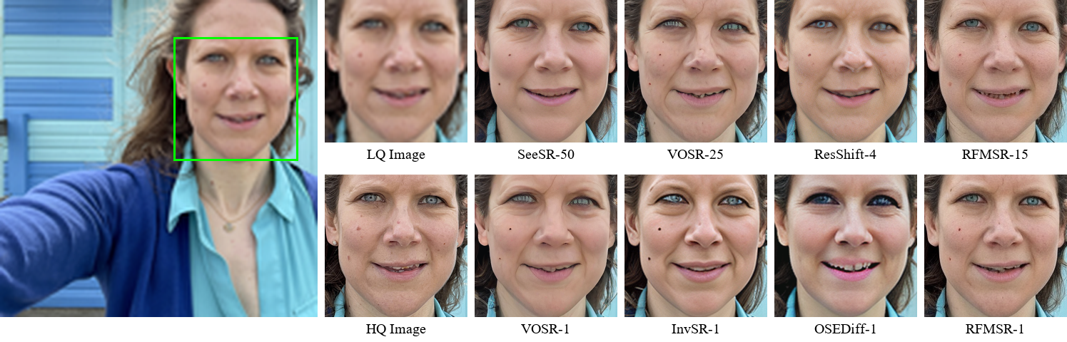
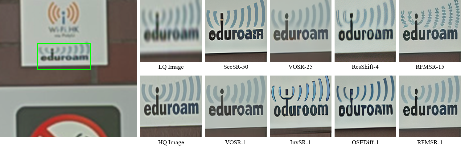
Figure 5: Visual comparison of RFMSR with state-of-the-art methods on real-world images. The number following each method name denotes its inference steps. (Zoom in for best view.).
| Method | Steps | PSNR\(\uparrow\) | SSIM\(\uparrow\) | LPIPS\(\downarrow\) | DISTS\(\downarrow\) | NIQE\(\downarrow\) | MUSIQ\(\uparrow\) | MANIQA\(\uparrow\) | CLIPIQA\(\uparrow\) | ||||||||||||||||
|---|---|---|---|---|---|---|---|---|---|---|---|---|---|---|---|---|---|---|---|---|---|---|---|---|---|
| w/o GAN | 1-step | 20.28 | 0.5154 | 0.1959 | 0.1270 | 3.9338 | 71.4848 | 0.5073 | 0.6858 | ||||||||||||||||
| 5-step | 20.33 | 0.5053 | 0.2162 | 0.1391 | 4.8056 | 71.9721 | 0.6024 | 0.7291 | |||||||||||||||||
| 15-step | 19.94 | 0.4881 | 0.2155 | 0.1315 | 4.0532 | 72.6567 | 0.5786 | 0.7334 | |||||||||||||||||
| w/o Velocity | 1-step | 19.91 | 0.5084 | 0.1992 | 0.1293 | 3.9933 | 72.2882 | 0.5266 | 0.7108 | ||||||||||||||||
| 5-step | 19.43 | 0.4862 | 0.2212 | 0.1457 | 4.7618 | 71.0794 | 0.4344 | 0.7081 | |||||||||||||||||
| 15-step | 18.99 | 0.4672 | 0.2745 | 0.1645 | 5.3089 | 68.5734 | 0.3987 | 0.6686 | |||||||||||||||||
| Phase II | 1-step | 20.10 | 0.5116 | 0.1961 | 0.1257 | 3.9389 | 71.7196 | 0.5182 | 0.7111 | ||||||||||||||||
| 5-step | 20.26 | 0.5027 | 0.2115 | 0.1360 | 4.6247 | 71.7807 | 0.5875 | 0.7373 | |||||||||||||||||
| 15-step | 19.91 | 0.4874 | 0.2124 | 0.1295 | 3.8866 | 72.4163 | 0.5533 | 0.7467 |
In this section, we analyze the design choices of the proposed method and evaluate its performance on three real-world datasets. We mainly focus on the \(\times 4\) ISR task following prior works. To simplify the presentation, we refer to our method as RFMSR, standing for Residual Flow Matching for Image Super-Resolution.
4.1 Experiment Settings↩︎
Training and Testing Datasets. To construct a diverse training set, we collect images from public sources including LSDIR [42], DIV2K [43], and Flickr2K, as well as web images subjected to quality filtering. In total, approximately 1M high-quality images are curated for training. We then synthesize HQ-LQ training pairs using the Real-ESRGAN degradation pipeline [7].
For evaluation, we adopt the RealSR test set [44], and randomly sample 250 images from the ImageNet [45] and LSDIR [42] test splits,
respectively. All HQ images are randomly cropped to \(512 \times 512\) resolution, then degraded through the Real-ESRGAN pipeline to produce \(128 \times 128\) LQ images.
Compared Methods. We compare RFMSR against representative real-world ISR methods, including multi-step approaches ResShift [22], SeeSR [17], and VOSR [24], as well as single-step methods OSEDiff [18], SinSR [23], InvSR [19], and the single-step distillation variant of VOSR [24]. Among these, SeeSR, OSEDiff, and InvSR are built upon large-scale T2I foundation models, while ResShift, VOSR, and SinSR are vision-only approaches.
All comparisons follow the official configurations of each method. For VOSR, we adopt its 0.5B-parameter variant. For our method, we report the multi-step variant of RFMSR, which is trained using only Phase I, and the single-step variant of RFMSR, which is
obtained after Phase II.
Evaluation Metrics. We evaluate all methods with full-reference and no-reference metrics. For distortion fidelity, we report PSNR and SSIM [38] on the Y channel of the YCbCr color space. For reference-based perceptual quality, we use LPIPS [39], DISTS [46], and FID [47]. For no-reference perceptual quality, we report NIQE [48], MUSIQ [49], MANIQA [50], and CLIPIQA [51].
Model Architecture. RFMSR adopts the model architecture of VOSR [24], the current SOTA vision-only ISR method. Specifically, it uses
LightningDiT [25] as the backbone with 0.5B parameters, the SD2.1 VAE [37] for image encoding, and DINOv2-Base [26] for semantic encoding. The model
takes the encoded LQ latent \(y_0\) and the DINOv2 semantic features as the joint conditioning input \(c = (y_0, \,\text{DINOv2}(\text{LQ Image}))\). In Phase I, we initialize the model from
the pre-trained VOSR weights.
For all experiments reported in the main text, the noise level is set to \(\sigma = 1.0\). Detailed training hyper-parameters and configurations are provided in the Appendix.
4.2 Experimental Results↩︎
Quantitative Comparisons. 1 reports the quantitative results on LSDIR, ImageNet-Test, and RealSR. In the multi-step setting, RFMSR achieves competitive or superior perceptual quality across all three benchmarks. On LSDIR, it attains the best full-reference and no-reference perceptual metrics including LPIPS, DISTS, MANIQA, and CLIPIQA, while maintaining competitive MUSIQ and FID. On ImageNet-Test, RFMSR achieves competitive no-reference perceptual quality and the best DISTS and NIQE among multi-step methods. On RealSR, it obtains the best PSNR and FID among all multi-step methods with competitive perceptual quality. Notably, despite using fewer steps, RFMSR consistently matches or exceeds SeeSR and VOSR in perceptual quality while maintaining reasonable distortion fidelity.
In the single-step setting, RFMSR demonstrates the effectiveness of our two-phase training strategy. RFMSR achieves significantly better LPIPS and DISTS than SinSR on LSDIR, with substantially improved FID. A similar trend holds on ImageNet-Test and
RealSR, where RFMSR consistently attains the best or second-best LPIPS, DISTS, and FID among all single-step methods. Compared with VOSR, RFMSR yields meaningful gains in perceptual quality across all datasets, demonstrating that the residual flow
formulation combined with two-phase training provides a stronger single-step baseline than standard flow matching and distillation approaches.
Qualitative Comparisons. 5 provides visual comparisons under both multi-step and single-step settings. For the portrait sample, OSEDiff, InvSR and VOSR exhibit local artifacts and unnatural rendering
in facial details, while SeeSR and ResShift produce over-smoothed textures; RFMSR achieves well-balanced texture recovery and structural fidelity. For the text logo, ResShift, OSEDiff, InvSR and SeeSR all produce distorted glyphs with misspelling and edge
blurring, whereas RFMSR and VOSR maintain accurate structural reconstruction. More visual comparisons are provided in the Appendix.
Comparison of Flow Matching Strategies. To validate the gains brought by our residual flow formulation, we compare it against the standard rectified flow [13] under identical training settings. Both strategies are trained purely via the conditional velocity matching loss. The standard rectified flow transports from a standard Gaussian prior \(x_1
\sim \mathcal{N}(0, I)\) to the HQ latent \(x_0\) along a straight-line path \(x_t = (1 - t)\,x_0 + t\,x_1\). The results are presented in 2.
The residual flow consistently outperforms the rectified flow across all metrics and step counts, in terms of both distortion fidelity (e.g., PSNR, LPIPS) and perceptual quality (e.g., MUSIQ, CLIPIQA). This advantage persists from low to high step counts,
and the gap remains stable across all evaluation settings. The consistent improvement can be attributed to centering the source distribution at \(y_0\), which shortens the transport path and preserves structural priors, in
contrast to the rectified flow that starts from pure Gaussian noise and must traverse a much longer trajectory.
Comparison of Single-Step Training Strategies. To evaluate the effectiveness of our proposed two-phase training paradigm for single-step generation, we compare Phase II against consistency learning [20], as reported in 3. The detailed implementation of consistency learning is provided in the
Appendix. As shown in the table, Phase I (pure CFM training) serves as a reference baseline with limited single-step quality. Consistency training achieves competitive single-step performance with strong perceptual metrics, demonstrating
the effectiveness of trajectory-level self-consistency constraints. However, its performance degrades sharply as the step count increases, with severe drops in both fidelity and perceptual quality at 5-step and 15-step inference. Moreover, it suffers from
a notable fidelity degradation compared to Phase I. Our Phase II maintains strong single-step fidelity on par with Phase I, and can further improve perceptual quality by increasing inference steps, confirming that jointly supervising the full trajectory
with end-to-end signals offers a superior trade-off between single-step efficiency and multi-step flexibility.
Ablation Study on Phase II Loss Functions. As shown in 4, removing the GAN loss (w/o GAN) yields the highest single-step fidelity, with marginal gains in PSNR and SSIM over the full Phase II, at the
expense of slightly lower perceptual quality. This suggests that the GAN loss primarily contributes to perceptual sharpness rather than pixel-level accuracy. Removing the velocity loss (w/o Velocity), however, degrades performance across the board. While
its single-step results remain relatively close to the full Phase II, the multi-step performance deteriorates substantially, with notable drops in both fidelity and perceptual metrics as the step count increases. This indicates that the velocity loss is
essential for preserving the flow-based generative prior and enabling meaningful multi-step refinement. The full Phase II, which combines the CFM velocity loss with LPIPS and GAN, achieves the best overall trade-off, maintaining strong single-step quality
while fully retaining multi-step inference capability.
Additional Studies. Further experimental results and details are provided in the Appendix.
5 Conclusion↩︎
In this paper, we revisited flow-matching-based image super-resolution and showed that an effective flow formulation is a key to high-quality generative restoration. Specifically, we proposed RFMSR, a vision-only ISR framework grounded in residual flow matching. By centering the source distribution at the LQ latent \(y_0\), the residual flow reduces the transport distance and preserves structural priors throughout the trajectory. A two-phase training strategy further equips the model with strong single-step generation while fully retaining multi-step inference capability. Extensive experiments on synthetic and real-world benchmarks demonstrate that RFMSR achieves competitive or superior perceptual quality compared to representative T2I-based ISR methods. Ablation studies confirm the effectiveness of the residual flow formulation and the two-phase training design.
Limitation. Our model architecture is designed based on the 0.5B-parameter variant of VOSR. Further scaling up the model capacity and training from scratch on larger datasets may yield additional performance improvements. The current framework is limited to the \(\times 4\) ISR setting and has not been validated on broader degradation types. Furthermore, incorporating more advanced end-to-end reconstruction losses, such as larger GAN discriminators or better perceptual losses, may further boost single-step generation quality. In future work, we will further investigate these issues.
6 Appendix↩︎
6.1 Training Details↩︎
A summary of the training hyper-parameters for Phase I and Phase II is provided in 5. Detailed descriptions of training configurations are given below.
| Hyper-parameter | Phase I | Phase II |
|---|---|---|
| Optimizer | AdamW | AdamW |
| Learning rate | \(5\times 10^{-5}\) | \(5\times 10^{-5}\) |
| \(\beta_1 / \beta_2\) | 0.9 / 0.999 | 0.9 / 0.999 |
| Weight decay | \(0.0\) | \(0.0\) |
| Learning rate schedule | - | - |
| Batch size | 32 | 16 |
| Training iterations | 10k | 10k |
| LQ size | \(128 \times 128\) | \(128 \times 128\) |
| HQ size | \(512 \times 512\) | \(512 \times 512\) |
| Noise level \(\sigma\) | 1.0 | 1.0 |
| \(\mathcal{L}(\theta)\) | ✔ | ✔ |
| \(\lambda_{\text{LPIPS}}\) | - | 1.0 |
| \(\lambda_{\text{GAN}}\) | - | 0.1 |
Phase I. We train the velocity field \(v_\theta\) using the AdamW optimizer [52] with \(\beta_1 = 0.9\), \(\beta_2 = 0.999\), and no weight decay. The learning rate is set to \(5\times 10^{-5}\) without a learning rate schedule. We use a batch size of \(32\) and train for \(10\)k iterations. The noise level \(\sigma\) is set to \(1.0\). HQ images are randomly cropped to \(512\times 512\), and the corresponding \(128\times 128\) LQ images are synthesized using the Real-ESRGAN degradation pipeline [7].
Phase II. We fine-tune the Phase I checkpoint for an additional \(10\)k iterations, using the same optimizer settings with a reduced batch size of \(16\). The LPIPS loss weight \(\lambda_{\text{LPIPS}}\) is set to \(1.0\) and the GAN loss weight \(\lambda_{\text{GAN}}\) is set to \(0.1\). The discriminator follows the PatchGAN [40] architecture with hinge loss [41].
Computational Resources. All training and inference experiments reported in this paper are conducted on a single NVIDIA RTX PRO 6000 GPU with 96GB of memory.
6.2 Alternative Single-Step Training Strategies↩︎
We implement consistency learning [20] as a representative single-step acceleration baseline for comparison with the proposed Phase II. It shares the same backbone architecture and residual flow formulation as RFMSR, and is initialized from the Phase I checkpoint.
Consistency Learning. Following Consistency Models [20], we define a consistency function \(f_\theta\) that directly maps any point on the residual flow trajectory to the clean HQ latent \(x_0\): \[f_\theta(x_t, t) = x_t - t \cdot v_\theta(x_t, t, c),\] which satisfies the boundary condition \(f_\theta(x, 0) = x\). The flow path follows the same formulation as RFMSR: \(x_t = x_0 + t\,(y_0 - x_0) + t\,\sigma\,\varepsilon\). During training, we sample a random timestep \(t \in [t_{\text{min}}, 1]\) and construct two adjacent trajectory points \(x_t\) and \(x_{t - \Delta t}\) using the same noise \(\varepsilon\) to ensure trajectory consistency. The online model predicts \(f_\theta(x_t, t)\), while a target model (an EMA of the online model with decay rate \(0.999\)) predicts \(f_{\theta^-}(x_{t - \Delta t},\, t - \Delta t)\). The consistency training loss enforces agreement between the two predictions: \[\mathcal{L}_{\text{CT}} = \mathbb{E}_{t, \varepsilon} \big[ \| f_\theta(x_t, t) - \text{sg}[f_{\theta^-}(x_{t - \Delta t},\, t - \Delta t)] \|^2 \big],\] where \(\text{sg}\) denotes stop-gradient. We set \(t_{\text{min}} = 10^{-3}\) to avoid numerical instability at \(t = 0\), and \(\Delta t = 0.05\). The target network is updated after each optimizer step via EMA, and the training runs for \(30\)k iterations with the same optimizer configuration.
| \(\sigma\) | PSNR\(\uparrow\) | SSIM\(\uparrow\) | LPIPS\(\downarrow\) | NIQE\(\downarrow\) | MUSIQ\(\uparrow\) | CLIPIQA\(\uparrow\) |
|---|---|---|---|---|---|---|
| 0.0 | 23.59 | 0.6747 | 0.4195 | 10.5745 | 55.4524 | 0.5887 |
| 0.5 | 24.09 | 0.6775 | 0.3082 | 5.72 | 64.1736 | 0.652 |
| 1.0 | 24.14 | 0.6755 | 0.3153 | 5.5898 | 63.2619 | 0.641 |
| 2.0 | 24.37 | 0.6899 | 0.3033 | 5.9319 | 61.202 | 0.596 |
6.3 Ablation Study on Noise Level↩︎
The noise level \(\sigma\) controls the initial perturbation strength around the LQ latent \(y_0\) in the residual flow formulation 1 . We train separate models with \(\sigma \in \{0.0, 0.5, 1.0, 2.0\}\) under the same training configuration until convergence, then evaluate all variants on the RealSR dataset using \(15\) uniform inference steps.
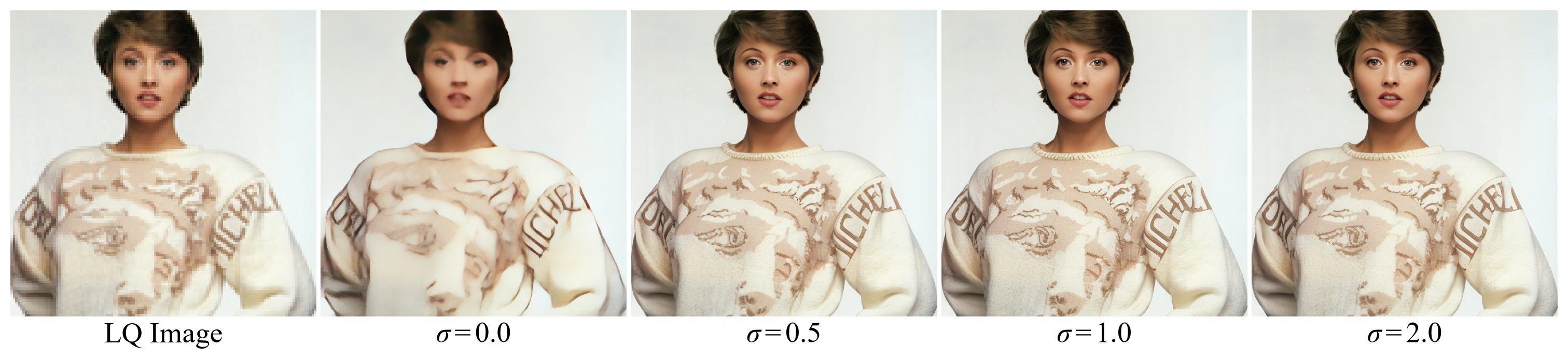
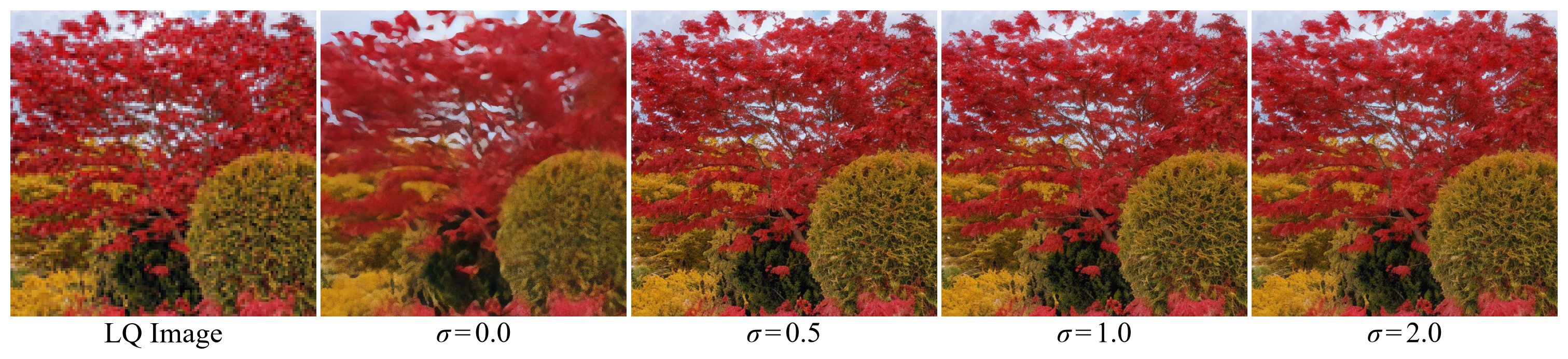
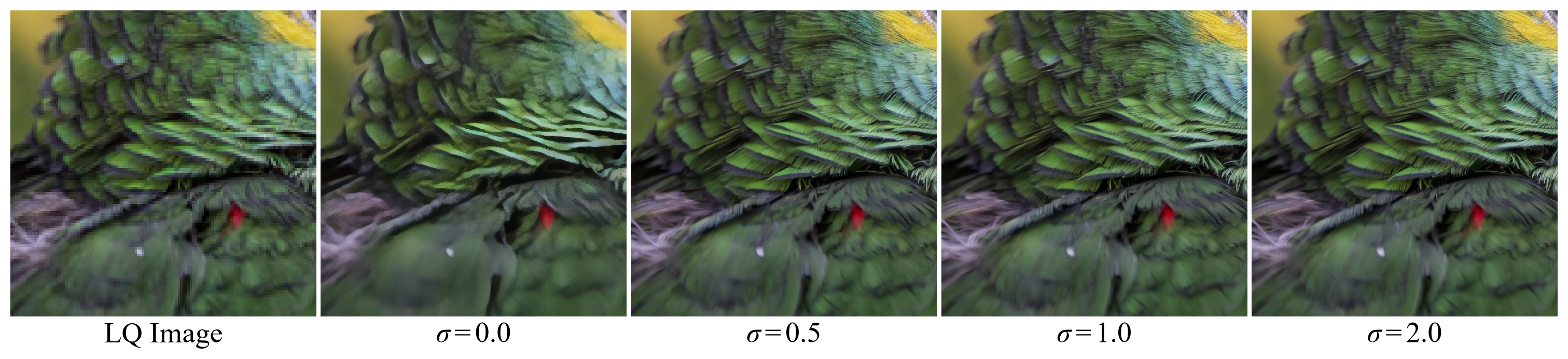
Figure 6: Additional visual examples of the noise level \(\sigma\) ablation. (Zoom in for best view.).
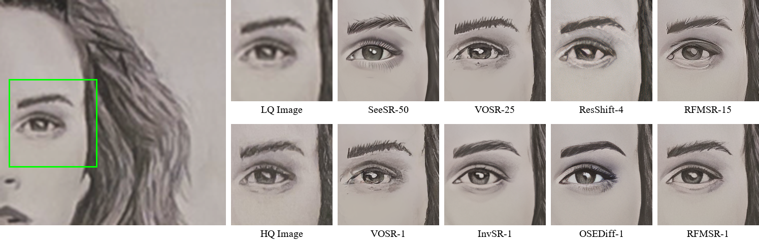
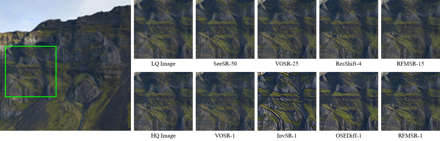
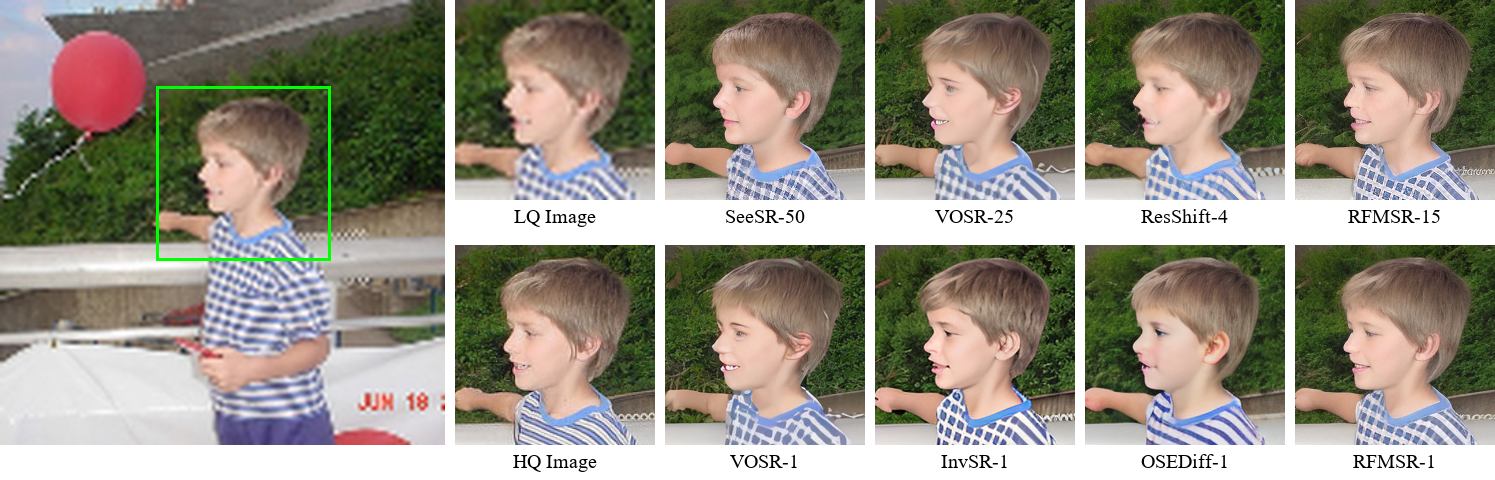
Figure 7: Additional visual comparisons of RFMSR with state-of-the-art methods on real-world images. (Zoom in for best view.).
As shown in 6, setting \(\sigma = 0.0\) reduces the residual flow to a deterministic \(\mathcal{L}_2\) regression, which achieves comparable fidelity metrics (PSNR and SSIM) but suffers from severe perceptual degradation across all perceptual indicators. Introducing a modest noise level (\(\sigma = 0.5\)) dramatically improves perceptual quality (e.g. MUSIQ, CLIPIQA), with substantial gains in LPIPS and NIQE. Further increasing \(\sigma\) to \(1.0\) or \(2.0\) yields additional gains in reconstruction fidelity (PSNR, SSIM) while maintaining good perceptual quality. We choose \(\sigma = 1.0\) as the default, as it provides a favorable trade-off between distortion fidelity and perceptual naturalness across all datasets. Additional visual comparisons are provided in 6.
6.4 Additional Visual Comparisons↩︎
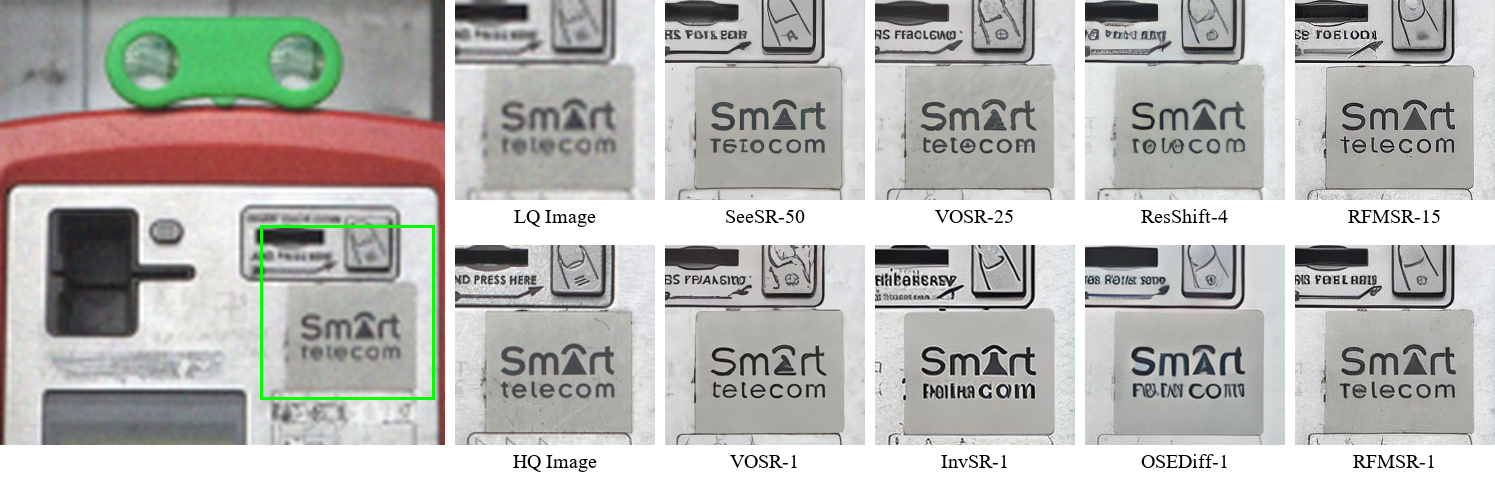
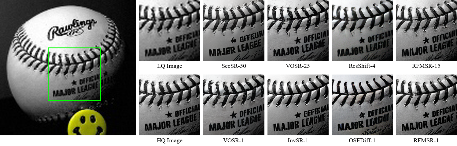
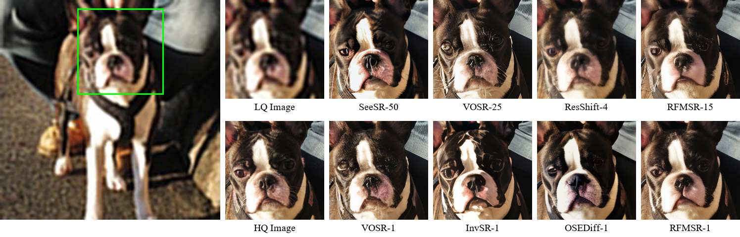
Figure 8: Additional visual comparisons of RFMSR with state-of-the-art methods on real-world images. (Zoom in for best view.).
As shown in 7 and 8, the additional visual comparisons cover a diverse range of scenarios including portrait details, natural landscapes, and text logos. Across all examples, RFMSR consistently produces results with the most natural texture and fewest artifacts among multi-step methods. Compared with SeeSR, which tends to over-smooth fine details, and ResShift, which occasionally introduces unnatural patterns, RFMSR preserves authentic structural fidelity while recovering rich textures. In the single-step setting, RFMSR demonstrates clear advantages over competing methods: VOSR produces plausible but slightly blurred outputs, while InvSR and OSEDiff frequently introduce local artifacts and distorted structures, particularly visible in the text logo and facial detail examples. Notably, RFMSR maintains accurate glyph reconstruction for text content and preserves fine-grained facial textures with high fidelity, confirming that the residual flow formulation combined with two-phase training provides a robust foundation for both high-quality single-step generation and progressive multi-step refinement.