Globalized Constrained Stein Variational Inference for Diverse Feasible Robot Motion Planning
July 14, 2026
Abstract
Robot motion planning is inherently multimodal, yet classical planners typically return only a single solution. Probabilistic formulations address this limitation by maintaining a distribution over motions, allowing the planner to reason over multiple low-cost alternatives. In robotics, however, motion samples must also satisfy strict constraints, including collision avoidance, joint limits, contact conditions, and dynamics consistency. These hard requirements make motion sampling substantially more challenging: within a limited planning budget, the ensemble must cover diverse low-cost motions while ensuring that every sample remains feasible under the relevant constraints. We propose SteinSQP (Stein Variational Sequential Quadratic Programming), a constrained Stein variational inference method for diverse feasible robot motion sampling. SteinSQP evolves an interacting particle ensemble, as in Stein variational methods, while embedding constraints directly into a kernel-space SQP subproblem. We solve the resulting constrained Stein–Newton subproblem with a GPU-friendly matrix-free primal–dual algorithm, enabling efficient batched ensemble updates. To globalize the method, we introduce an ensemble-level merit function that jointly balances objective value, constraint violation, and particle diversity. Across five constrained motion-planning tasks, SteinSQP returns fully feasible ensembles while preserving diverse motion alternatives. Compared with first-order constrained Stein baselines and serial multistart nonlinear programming, SteinSQP shows faster and more robust ensemble convergence in terms of iterations, improves particle-wise feasibility, and achieves faster batched time-to-solution on challenging robot-scale tasks.
Constrained Stein variational inference, Sampling as Constrained Optimization, Constrained motion planning.
1 Introduction↩︎
Robot motion planning is conventionally formulated as the search for a single trajectory that minimizes a cost functional subject to hard constraints such as joint limits, collision avoidance, and contact conditions [1], [2]. Yet a single minimizer discards structure that most tasks naturally possess: a manipulator can pass an obstacle on either side, a throw can be released from different arm configurations, and a push can exploit different contact faces. A planner committed to one solution is brittle precisely where planning matters most. It is easily trapped in a poor local optimum, and it offers no fallback when the environment changes, when a downstream module rejects the trajectory, or when execution fails. What is needed instead is a set of low-cost, feasible, and qualitatively distinct motions, produced within a single planning budget.
Casting motion optimization as probabilistic inference provides precisely this structure [3], [4]. The objective induces a distribution over the optimization landscape, with high-density regions concentrated near distinct local optima of the underlying nonlinear program, while hard constraints restrict its support to the feasible set: a manifold under equality constraints, or a domain with boundary under inequalities. Sampling from this constrained distribution therefore returns a diverse collection of feasible motions in one solve, rather than a single point estimate. The difficulty is computational. The samples must be simultaneously low-cost, feasible with respect to nonlinear equality and inequality constraints, diverse, and they must be obtained fast enough to be useful for planning.

Classical constrained samplers fall short of this requirement because they are inherently sequential. Manifold MCMC methods [5] are asymptotically exact, but rely on long mixing chains and do not share information across samples. Constraint-manifold RRTs [6], [7] similarly expand one projected node at a time. Neither maps well onto the parallel hardware that modern robot software stacks are built around. Stein Variational Gradient Descent (SVGD) [8] does. It evolves an entire ensemble of interacting particles in parallel, each driven toward low cost while a pairwise repulsion prevents collapse onto a single solution: in effect, a batched multi-start optimizer whose restarts communicate. SVGD, however, assumes an unconstrained domain. Its constrained extensions either apply only to restricted constraint classes, namely convex sets via mirror maps [9] or a single equality manifold via projected kernels [10], or handle nonlinear inequalities indirectly, through squared slack variables [11] or penalty and augmented-Lagrangian terms [12]. These reformulations share a common defect: they alter the particle flow precisely at active constraint boundaries, where feasibility is most delicate, introducing spurious local optima and distorting the empirical distribution of the ensemble exactly where the constrained posterior concentrates.
In this article we take a different route: rather than reformulating the constraints, we make each Stein step feasible by construction. Inspired by the interpretation of constrained SVGD as SQP [13] and by safe particle flows [14], we linearize the constraints at the current ensemble and enforce them directly on the kernel-coupled ensemble displacement via a quadratic program (QP). This lets equality and inequality constraints enter the particle flow at first order, without slack variables or hand-tuned penalties. Three observations turn this idea into a practical solver. First, the same QP can incorporate second-order curvature information, such as Gauss–Newton approximations, upgrading the safe first-order flow to a constrained Stein–Newton update. This improves convergence speed while preserving constraint satisfaction, rather than merely enforcing feasibility. Second, although the kernel coupling makes the QP’s KKT system dense and prohibitive to factorize, a primal–dual hybrid gradient scheme (PDHG) [15], [16] that never forms this system solves it using only kernel products and small independent per-particle solves, a computational pattern that GPUs execute almost natively. Third, a QP step trusts a linearization and must therefore be globalized. Prior constrained Stein methods either omit globalization entirely or line-search on objective alone, which collapses the very modes the ensemble exists to preserve. We instead globalize with an ensemble-level merit function that balances the three goals a constrained sampler must serve simultaneously: low cost, constraint satisfaction, and transport diversity. By tailoring globalization to the Stein particle flow, this mechanism safeguards ensemble diversity while steering particles toward feasible, low-cost regions.
We call the resulting method SteinSQP: an SQP-like particle optimizer that turns constrained Stein transport into a practical GPU-parallel solver for multimodal nonlinear programs. We summarize our contributions as follows:
Constrained Stein–Newton updates in kernel space. We formulate an SQP-like Stein variational Newton step that embeds linearized equality and inequality constraints directly into the kernel-coupled ensemble displacement, avoiding slack variables, fixed penalties, and post-hoc projection.
A GPU-parallel primal–dual solver. We solve the dense kernel-coupled QP without forming or factorizing its KKT system, using only kernel products and independent per-particle solves. The resulting dual iterates also provide the exact-penalty weight used by the merit function, eliminating a fragile hand-tuned parameter.
Stein-aware globalization. We introduce an ensemble-level merit function for constrained Stein updates that jointly accounts for cost, feasibility, and transport diversity, together with a second-order correction to mitigate Maratos-type stalling.
Empirical validation on robot-scale tasks. Across five benchmarks, SteinSQP achieves fully feasible ensembles while improving robustness and batched wall-clock time over both first-order Stein and serial multistart NLP baselines. It also shows a faster outer-iteration convergence than serial multistart NLP.
The remainder of this article is organized as follows. Section 2 reviews constrained sampling for motion planning and constrained Stein variational inference. Section 3 formalizes the constrained posterior sampling problem, and Section 4 recalls the necessary background on kernel transport maps and Stein variational inference. Section 5 develops SteinSQP, Section 6 presents the experimental evaluation, and Section 7 concludes.
2 Related Work↩︎
2.1 Constrained Sampling for Robot Motion Planning↩︎
Casting motion optimization as probabilistic inference lets a planner reason about a distribution of low-cost motions rather than a single minimizer [3], [4]. When hard constraints are present, this posterior is supported on a lower-dimensional feasible set, and the central difficulty becomes drawing diverse samples that remain feasible. Sampling-based planners address this geometrically: projection-based methods repeatedly retract configurations onto the constraint manifold [6], while Tangent Space RRT [7] and Tangent Bundle RRT [17] grow trees in local tangent charts. Both incur high projection cost and struggle with strongly nonlinear constraints. A complementary line treats the feasible set as an implicitly defined manifold and applies manifold MCMC: constrained Hamiltonian Monte Carlo with RATTLE-type symplectic integrators [5], [18], Riemann manifold HMC [19], and geodesic Monte Carlo [20]. These schemes are asymptotically exact but rely on sufficient chain mixing, share no information across samples, and are hard to parallelize, which limits their use under tight planning budgets. Closer to our setting, combining Gauss–Newton constraint satisfaction with interior sampling produces diverse constrained samples [21], but still proceeds sequentially, while learned generative models amortize manifold sampling [22] at the cost of training data and poor generalization to unseen constraints. In contrast, particle-based variational inference evolves an interacting ensemble jointly, coupling samples through a repulsion term so that diversity and feasibility are pursued in parallel, the regime our method targets.
2.2 Constrained Stein Variational Inference↩︎
Stein Variational Gradient Descent (SVGD) [8], [23] approximates a target by a set of interacting particles that follow the steepest KL-descent field in an RKHS, balancing a score-driving term against a repulsion term, and can be viewed as a gradient flow of the KL divergence [24]. Second-order variants precondition this flow: the Stein Variational Newton (SVN) method [25] approximates a Newton iteration in function space, and related second-order Stein schemes have since been applied to dynamic optimization and control [26]. Extending SVGD to constrained supports has followed three broad strategies. Mirror-map methods evolve particles in a dual space to remain within convex constraints [9]; moment-constraint approaches enforce expectation constraints through a primal–dual flow [27]; and projection methods build the constraint into the function space itself. In particular, Orthogonal-space SVGD (O-SVGD) [10] uses a projected matrix-valued kernel whose fields are tangent to a single equality manifold, while functional gradient flows with boundary conditions confine particles to general domains with convergence guarantees [28]. Further extensions, such as Riemannian SVGD [29] and Lie-group SVGD [30], are tailored primarily to intrinsic manifold constraints, but may be less straightforward to deploy in general-purpose applications.
In robotics, these ideas underpin recent constrained trajectory samplers. CSVTO [11] extends O-SVGD to multiple equality and inequality constraints with a tangent-space resampling step, but handles inequalities through squared slack variables, which, as that work notes, introduce many spurious local optima and distort the empirical distribution near active boundaries. Safe particle flow [13], [14] instead enforces linearized inequalities via a control-barrier quadratic program, and augmented-Lagrangian formulations of constrained SVGD handle arbitrary constraints at the cost of penalty tuning [12]. What remains open is a method that treats nonlinear inequalities directly, without slack variables or fixed penalties, while retaining a globalized, curvature-aware Stein flow that parallelizes across particles. SteinSQP targets exactly this gap: each Stein proposal is embedded in an SQP subproblem solved in kernel space and globalized by an exact-penalty line search, with the inner saddle-point problem handled by a matrix-free primal–dual scheme that maps well onto GPU hardware.
3 Problem Definition↩︎
A Boltzmann distribution formulation casts optimization-based robot motion optimization as probabilistic inference. Let \(x\) denote a finite-dimensional motion variable, which may represent robot configuration parameters or a trajectory in generalized coordinates. Given a prior distribution \(p_0(x)\), the likelihood takes the form \(l(x) \propto \exp(-V(x)/T)\), where \(V(x)\) denotes the motion-level cost and \(T>0\) controls the temperature. This formulation yields the posterior distribution \(p(x) \propto p_0(x)\exp(-V(x)/T)\). As \(T \to 0\), the posterior concentrates on the minimum-cost motions within the support of \(p_0(x)\), recovering deterministic motion optimization in the zero-temperature limit.
We consider a general constrained nonlinear program with a nonlinear least-squares objective \(V(x)=\tfrac{1}{2}\|r(x)\|^2\), where \(r:\mathbb{R}^d\to\mathbb{R}^{m_r}\) is a smooth residual map. The feasible set is defined as \(\mathcal{F}\doteq \{x \mid h(x)=0,\;g(x)\leq 0\}\), where \(h:\mathbb{R}^d\to\mathbb{R}^{m_h}\) and \(g:\mathbb{R}^d\to\mathbb{R}^{m_g}\) denote equality and inequality constraint functions, respectively, with the inequality applied elementwise. This formulation covers a wide range of robotics motion planning tasks, such as motion planning with obstacle avoidance. Moreover, even when contact dynamics are involved, they can be handled via relaxation and smoothing techniques to enable a nonlinear programming formulation, further broadening the applicability of this formulation.
To incorporate feasibility, we introduce the extended-value indicator \(\iota_{\mathcal{F}}(x)\), where \(\iota_{\mathcal{F}}(x)=0\) if \(x\in\mathcal{F}\) and \(\iota_{\mathcal{F}}(x)=+\infty\) otherwise. The constrained Boltzmann likelihood induced by \(V(x)+\iota_{\mathcal{F}}(x)\) is equivalent to \(\exp(-V(x)/T)\,\mathbf{1}_{\mathcal{F}}(x)\), where \(\mathbf{1}_{\mathcal{F}}(x)\) is the binary feasibility indicator. The target posterior is therefore given by \[\label{eq:constrained95posterior} \pi(x) \propto p_0(x)\exp \bigl(-V(x)/T\bigr) \, \mathbf{1}_{\mathcal{F}}(x),\tag{1}\] which assigns zero density to infeasible motions.
Our goal is to draw samples from this constrained posterior, where each sample represents a feasible robot motion and different modes correspond to distinct local optima. This perspective positions sampling not only as a means of approximating the posterior, but also as a mechanism for uncovering multiple high-quality local modes. We therefore seek a method that achieves a favorable trade-off among sampling efficiency, sample diversity, and fidelity to the constrained target distribution.
In the context of Stein variational inference, this objective requires a Stein operator that respects the constrained motion domain. We introduce the necessary preliminaries in the next section.
4 Preliminaries↩︎
This section introduces notation and recalls the three ingredients our method builds on: reproducing-kernel function spaces, Stein variational inference viewed as optimization over a particle ensemble, and the enforcement of equality constraints as a tangency condition on the ensemble’s transport field.
4.1 Kernel Spaces and Transport Maps↩︎
Let \(k:\mathbb{R}^d\times\mathbb{R}^d\to\mathbb{R}\) be a positive-definite kernel and \(\mathcal{H}_k\) its scalar reproducing-kernel Hilbert space (RKHS); \(\mathcal{H}\doteq \mathcal{H}_k^d\) denotes the corresponding space of vector fields \(\delta:\mathbb{R}^d\to\mathbb{R}^d\) with componentwise inner product. Two properties matter here. First, the reproducing property: for any \(\delta\in\mathcal{H}\), \(\left\langle \delta,\, k(x,\cdot)v\right\rangle_{\mathcal{H}} = \delta(x)^\top v\), so function evaluations are inner products and first-order calculus in \(\mathcal{H}\) has closed form. Second, given particles \(X=\{x_i\}_{i=1}^N\), the finite-dimensional span \[\label{eq:kernel95span} \delta(\cdot)\;=\;\sum_{j=1}^{N} k(\cdot,x_j)\,c_j, \qquad c_j\in\mathbb{R}^d,\tag{2}\] is the natural search space for ensemble updates: by the representer argument, the optimizer of any regularized functional that touches the particles only through \(\{\delta(x_i)\}\) lies in this span. Writing \(K\in\mathbb{R}^{N\times N}\), with \(K_{ij}=k(x_i,x_j)\) for the Gram matrix and stacking coefficients row-wise into \(C\in\mathbb{R}^{N\times d}\), the field values at the particles are \(D = KC\) and the RKHS norm is \(\left\lVert \delta\right\rVert_{\mathcal{H}}^2=\operatorname{tr}(C^\top K C)\).
A vector field \(\delta\) induces the transport map \(T_{\varepsilon}(x) = x + \varepsilon\,\delta(x)\), which carries an ensemble with density \(\rho\) to a new density \(\rho_\varepsilon\). For small \(\varepsilon\), where \(T_\varepsilon\) is invertible, the transported density satisfies \[\begin{align} \label{eq:pushforward} \log \rho_\varepsilon\bigl(T_\varepsilon(x)\bigr) = \log\rho(x) - \log\bigl|\det\bigl(I + \varepsilon\,\nabla \delta(x)\bigr)\bigr|, \end{align}\tag{3}\] so the log-determinant of the transport Jacobian measures the local change in ensemble volume, and hence in entropy. This term reappears twice in our method: implicitly, in the repulsion force of the Stein update, and explicitly, in the merit function of our ensemble line search (Section 5.4).
4.2 Stein Variational Inference as Ensemble Optimization↩︎
Let \(\pi\) be a target density on \(\mathbb{R}^d\). Sampling from \(\pi\) can be phrased as minimizing the KL divergence \(\mathrm{KL}(\rho\,\|\,\pi)\) over the ensemble density \(\rho\). SVGD performs this minimization by steepest descent restricted to \(\mathcal{H}\): among all function perturbations \(T_\varepsilon = \mathrm{id} + \varepsilon\delta\) with \(\left\lVert \delta\right\rVert_{\mathcal{H}}\le 1\), the one that instantaneously decreases the KL fastest is \[\label{eq:svgd95field} \delta^{\star}_{\rho}(\cdot) \;\propto\; \mathbb{E}_{x\sim\rho}\bigl[\,k(x,\cdot)\,\nabla_x\log\pi(x) \;+\;\nabla_x k(x,\cdot)\,\bigr],\tag{4}\] the kernelized Stein operator applied to \(\rho\). Instantiating this at the \(N\) particles gives the practical update: for each particle \(x_i\), \[\begin{align} \label{eq:svgd95empirical} \phi(x_i) = \underbrace{\frac{1}{N}\sum_{j=1}^N k(x_j,x_i)\,\nabla\log\pi(x_j)}_{\text{driving}} + \underbrace{\frac{1}{N}\sum_{j=1}^N \nabla_{x_j} k(x_j,x_i)}_{\text{repulsion}}, \end{align}\tag{5}\] where the first term transports probability mass toward high-density regions and the second, the derivative of the volume term in 3 through the kernel, pushes particles apart and is what prevents the ensemble from collapsing onto a single mode. Two refinements are standard. Second-order (Stein–Newton) methods precondition the field with a curvature model of \(-\log\pi\), either by a global Newton system in the span 2 or by cheaper block-diagonal approximations. Matrix-valued kernels replace \(k(x,y)\) by \(\mathcal{K}(x,y)\in\mathbb{R}^{d\times d}\), which allows the geometry of the target to enter the function space itself; we use this device for equality constraints below. Finally, the balance between driving and repulsion in 5 is exactly a temperature: annealing it trades exploration against exploitation. The abstraction to retain is this: an SVGD-type algorithm is an optimization method whose iterate is the whole ensemble, whose search direction is a vector field in \(\mathcal{H}\) sampled at the particles, and whose objective couples an averaged cost to an entropy regularizer, \[\label{eq:free95energy} E(\rho) \;=\; \mathbb{E}_{x\sim\rho}\bigl[V(x)\bigr] \;-\; \gamma\, H(\rho),\tag{6}\] where \(H(\rho)=-\mathbb{E}_{\rho}[\log\rho]\) is the ensemble entropy and the temperature \(\gamma>0\) sets their trade-off: the driving term reduces the average cost \(\mathbb{E}_\rho[V]\), while the repulsion increases the entropy \(H\) and keeps the particles spread out. Every globalization decision in Section 5 (what the line search measures, what “convergence” means for an ensemble that never stops jittering) is made against this ensemble objective, not against any single particle’s cost.
4.3 Equality Constraints as Tangency Conditions↩︎
Constraining a sampler is not the same as constraining an optimizer: what must respect \(\mathcal{F}\) is the entire ensemble, and it must do so along the whole flow, not only at the solution. For the equality part \(\mathcal{M}=\{x : h(x)=0\}\) of the feasible set, keeping every particle on \(\mathcal{M}\) at all times is equivalent to requiring the transport field to be tangent: \(J_h(x)\,\delta(x)=0\) on \(\mathcal{M}\), where \(J_h=\partial h/\partial x\). Prior work realizes this in one of three ways: reparameterizing the domain through a mirror map; splitting the field into tangential and normal components and using the normal one only to decay the constraint residual; or ignoring tangency during the Stein step and projecting particles back afterwards. The device we adopt is the projected matrix-valued kernel (the orthogonal kernel of [10]), later used for trajectory optimization (TO) in [11]. Let \[\label{eq:tangent95projector} P(x) \;=\; I - J_h(x)^\top\bigl(J_h(x)J_h(x)^\top + \epsilon I\bigr)^{-1}J_h(x)\tag{7}\] be the (regularized) orthogonal projector onto the tangent space of \(\mathcal{M}\) at \(x\). Then \[\label{eq:projected95kernel} \mathcal{K}_P(x,y) \;=\; P(x)\,k(x,y)\,P(y)\tag{8}\] is a positive-semidefinite matrix-valued kernel whose RKHS contains only fields that are pointwise tangent at the particles. Substituting \(\mathcal{K}_P\) for \(k\) in 4 projects the score and the repulsion of each source particle by its own \(P(x_j)\) before the kernel average, and the assembled field at each target by \(P(x_i)\) after it: the two projections do not commute with the sum and both are required.
As is conventional in constrained SVGD, the curvature term \(\nabla\!\cdot\!P\) of the manifold is dropped [11]. The result is a diversity flow that slides along the equality manifold: it never spends its budget fighting the constraints, and it never undoes the feasibility that the optimization layer (Section 5) establishes in the normal directions. Inequality constraints receive no such reparameterization; their handling is precisely where our method departs from prior work, through the SQP subproblem of Section 5.2 rather than the squared slack variables of [11], which introduce spurious local optima near active boundaries.
5 Method: SteinSQP↩︎
Handling nonlinear constraints in constrained SVGD via sequential quadratic programming was first introduced in [13] and later analyzed in detail from the perspective of safe particle flows in [14]. It keeps the two useful ingredients of SVGD, descent toward low-cost motions and repulsion between particles, but does not rely on an exact constrained Stein operator. Instead, every Stein-like proposal is made safe by an SQP subproblem and by a line search that re-evaluates the nonlinear constraints before accepting the step.
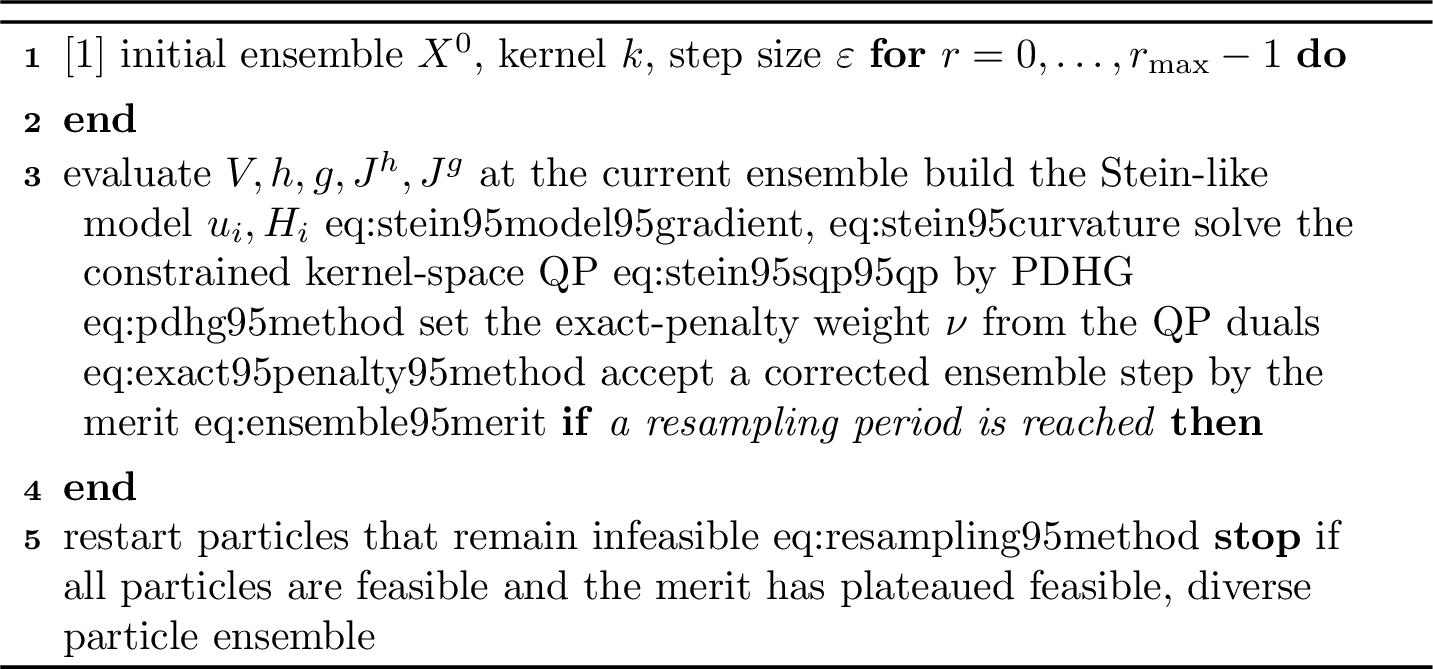
Let \(X=\{x_i\}_{i=1}^N\) be the current ensemble, with \(x_i\in\mathbb{R}^d\). The objective is \(V(x)=\tfrac12\left\lVert r(x)\right\rVert^2\), the score direction is \(s_i=-\nabla V(x_i)\), and the Gauss–Newton curvature is \(G_i=J_r(x_i)^\top J_r(x_i)\). Equality and inequality constraints are written as \(h(x)=0\) and \(g(x)\le0\), with Jacobians \(J_i^h\) and \(J_i^g\) at particle \(i\). One SteinSQP iteration has four steps: build a kernelized Stein descent model, solve a constrained quadratic subproblem in kernel space, globalize the resulting ensemble transport, and restart particles that remain in infeasible basins.
5.1 A Stein-Like Descent Model↩︎
5.1.1 Particle field↩︎
For a scalar kernel \(k\) with Gram matrix \(K_{ij}=k(x_i,x_j)\), the practical SVGD field at particle \(i\) is split into a driving term and a repulsion term, \[\begin{align} \label{eq:stein95forces} b_i &= \frac{1}{N}\sum_{j=1}^N K_{ji}\,s_j, \notag\\ \rho_i &= \frac{1}{N}\sum_{j=1}^N \nabla_{x_j} k(x_j,x_i). \end{align}\tag{9}\] The direction used by SteinSQP is \[\label{eq:stein95model95gradient} u_i = b_i+\gamma\rho_i ,\tag{10}\] where the temperature parameter \(\gamma\) controls the strength of diversity. The first term pulls the ensemble toward lower objective values; the second prevents collapse to a single local solution. We use this field as a computational descent direction for particles, not as an exact constrained sampling operator.
For equality constraints, an optional local tangent projection can be applied: the projector \(P_i=P(x_i)\) of 7 replaces \(s_j\) and \(\nabla_{x_j}k\) in 9 by their projected versions and projects the final field, recovering the orthogonal SVGD of [11] (Section 4.3). This is only a local safeguard that biases the flow along the equality tangent space; nonlinear feasibility is still enforced by the SQP and line-search layers below.
5.1.2 Curvature model↩︎
Following the Stein Variational Newton (SVN) method [25], the Stein-like field is preconditioned by a curvature model of \(-\log\pi\); we use its cheaper block-Jacobi approximation. For each particle, \[\begin{align} \label{eq:stein95curvature} H_i &= \frac{1}{N}\sum_{j=1}^N K_{ji}^2 G_j \nonumber \\ &+\frac{\gamma}{N}\sum_{j=1}^N \nabla_{x_j}k(x_j,x_i)\nabla_{x_j}k(x_j,x_i)^\top +\lambda I . \end{align}\tag{11}\] If tangent projection is used, the Gauss–Newton blocks and kernel gradients are projected before entering 11 . The damping \(\lambda I\) keeps the proximal systems positive definite. This approximation keeps only per-particle blocks, so the method avoids a coupled \(Nd\times Nd\) Newton system while still coupling particles through \(K\).
5.1.3 Trajectory kernels↩︎
For low-dimensional problems we use an RBF kernel. For trajectory variables, we use an RBF under a fixed acceleration metric, \[\begin{align} \label{eq:structured95rbf95method} k(x,y)&=\exp\!\left( -\frac{(x-y)^\top M(x-y)}{2\hbar}\right), \notag\\ M&=\alpha I+\beta D_2^\top D_2 , \end{align}\tag{12}\] where \(D_2\) is the second-difference operator over trajectory knots and \(\hbar>0\) is the kernel bandwidth. This kernel measures similarity between whole trajectories under an acceleration metric rather than the Euclidean distance between stacked coordinates: through \(D_2^\top D_2\), it compares neighboring knots and so penalizes differences in curvature, treating two motions as similar when they bend alike rather than merely passing through nearby points. The identity term is important: without it, offsets and ramps lie in the null space of \(D_2^\top D_2\) and the kernel becomes insensitive to some motion modes.
5.2 Constrained Kernel-Space Step↩︎
SteinSQP searches for an update field in the kernel span. Let \(C=(c_1,\ldots,c_N)^\top\in\mathbb{R}^{N\times d}\) be the coefficients and define the particle update direction \[\label{eq:kernel95direction95method} d_i=(\mathcal{K} C)_i=\sum_{j=1}^N K_{ij}c_j ,\tag{13}\] with the projected-kernel version used when equality projection is enabled. The coefficients \(C\) are chosen by the SQP subproblem \[\label{eq:stein95sqp95qp} \begin{align} \min_C\quad &\sum_{i=1}^N \left(\tfrac12 c_i^\top H_i c_i-u_i^\top c_i\right)\\ \mathrm{s.t.}\quad &h_i+\varepsilon J_i^h d_i=0,\\ &g_i+\varepsilon J_i^g d_i\le0, \qquad i=1,\ldots,N . \end{align}\tag{14}\] The constraints are imposed on the particle displacement \(d_i\), not on the coefficient \(c_i\). This matters because particles interact through the kernel: the same coupling that spreads the ensemble also appears in the linearized constraints. Equalities and inequalities are kept separate. Writing an equality as two inequalities would create linearly dependent active rows at every feasible point and unstable penalty multipliers.
5.3 Inner Solve without Forming the KKT System↩︎
At each outer iteration the SteinSQP direction is the minimizer of the quadratic subproblem 14 , posed not in the particle positions but in the RKHS coefficients \(C=(c_1,\dots,c_N)\) that generate the transport field \(\phi(x_i)=\sum_j k(x_i,x_j)\,c_j\): the joint displacement of all particles is \(\varepsilon\,\mathcal{K} C\), where \(\mathcal{K}\) is the kernel Gram operator, \(c_i\in\mathbb{R}^d\) the coefficient block of particle \(i\), and \(\varepsilon\) the SQP step scale. The subproblem minimizes the block-separable model \(\sum_i\!\bigl(\tfrac12 c_i^\top H_i c_i-u_i^\top c_i\bigr)\), in which \(u_i\) is the Stein variational gradient of particle \(i\) (its downhill score-driving pull plus the inter-particle repulsion) and \(H_i\succ0\) the corresponding block-Jacobi curvature model of 11 , subject to the constraints linearized about the current particles, \(h+B_h C=0\) and \(g+B_g C\le0\). Here \(h,g\) are the equality/inequality residuals, \(J^h,J^g\) their Jacobians, and \[B_h C=\varepsilon J^h\mathcal{K} C,\qquad B_g C=\varepsilon J^g\mathcal{K} C\] push a coefficient perturbation through the kernel into constraint space; we stack them as \(B=\bigl[\begin{smallmatrix}B_h\\ B_g\end{smallmatrix}\bigr]\).
Because the kernel couples all \(N\) particles, forming and factorizing the dense KKT system of this QP is prohibitive on a GPU. Even with a block-diagonal approximation, the Gram matrix still couples the per-particle constraints, preventing the subproblem from decomposing into independent particle-wise solves. We therefore dualize the constraints and solve the resulting convex–concave saddle problem with the primal–dual scheme of Chambolle and Pock [15], [16], which needs only applications of \(B\) and \(B^\top\) and leaves the primal step separable. Introducing an equality dual \(\lambda\) and a nonnegative inequality dual \(\mu\ge0\) (its sign enforces the KKT condition of \(g\le0\)), an extrapolated coefficient \(\bar C\), and primal and dual step sizes \(\tau,\sigma>0\), one inner iteration is \[\tag{15} \begin{align} \lambda^{+} &= \lambda+\sigma(B_h\bar C+h), \tag{16}\\ \mu^{+} &= \bigl[\mu+\sigma(B_g\bar C+g)\bigr]_+, \tag{17}\\ \tilde{C} &= C-\tau B^\top \begin{bmatrix}\lambda^{+}\\ \mu^{+}\end{bmatrix}, \tag{18}\\ c_i^{+} &= (I+\tau H_i)^{-1}(\tilde{c}_i+\tau u_i), \tag{19}\\ \bar C^{+} &= C^{+}+\theta(C^{+}-C). \tag{20} \end{align}\] Steps 16 –17 take a gradient ascent of the duals toward feasibility of the linearized constraints, with \(\sigma\) the dual step; the clamp \([\,\cdot\,]_+\) is the proximal operator of the constraint \(\mu\ge0\), i.e. a projection onto the nonnegative orthant. Steps 18 –19 form the primal gradient step \(\tilde{C}\) (with primal step \(\tau\)) and apply the proximal operator of the objective quadratic; since \(H=\operatorname{diag}(H_i)\) is block diagonal, this prox decouples into \(N\) independent \(d\times d\) SPD solves, one per particle, done in parallel. Because \(H_i\) and \(\tau\) are fixed across the inner loop, each \((I+\tau H_i)^{-1}\) is factorized once and reused for every inner iteration, so the prox is cheap. Step 20 is the over-relaxation that gives the scheme its accelerated, provably convergent rate. The step sizes must satisfy the PDHG stability bound \(\tau\sigma\lVert B\rVert^2\le1\): we fix \(\tau\) from a bound on \(\lVert H\rVert\) (so each prox is well conditioned) and take \(\sigma\) to saturate the bound up to a safety factor, estimating the coupling norm \(\lVert B\rVert\) by a few power-iteration sweeps of \(B^\top B\), never assembling \(B\), only applying \(\mathcal{K},\,J^h,\,J^g\) and their adjoints. Thus no KKT matrix is ever formed or factorized: each of the fixed number of inner iterations costs a handful of matrix-free operator applications plus \(N\) tiny per-particle solves, giving \(O(Nd)\) memory and an inner solve that parallelizes across particles. This is the root reason SteinSQP is efficient on a GPU: PDHG needs only dense kernel and Jacobian products and per-particle solves, exactly the regular, batched operations GPUs are built for.
We did explore exploiting the sparsity of the constraint Jacobians instead, but found it does not pay off: in our tests a sparse QP solver ran at least an order of magnitude or more slower on GPU, as sparse factorization maps poorly onto the hardware and its irregular structure outweighs the benefit of the reduced flop count. A dense matrix-free PDHG sweep, by contrast, keeps every operation regular and fully parallel, so we use it rather than a sparse QP solver for this subproblem.
5.4 Globalization↩︎
The SQP subproblem only sees a linearized model. A step is accepted only after testing the nonlinear objective and constraints. Let \(\Delta_i=\varepsilon d_i\) and let \(\Phi_i=\partial\Delta_i/\partial x_i\) be the Jacobian of the particle transport. For a candidate step length \(\alpha\), the line search evaluates \[\label{eq:corrected95candidate} y_i(\alpha)=x_i+\alpha\Delta_i+s_i(\alpha),\tag{21}\] where \(s_i(\alpha)\) is a second-order correction defined below. The accepted step is selected by the ensemble merit \[\begin{align} \label{eq:ensemble95merit} M(\alpha)={}& \frac{1}{N}\sum_i V(y_i(\alpha)) -\gamma\frac{1}{N}\sum_i\log\det(I+\alpha\Phi_i) \notag\\ &+\nu\frac{1}{N}\sum_i \left(\left\lVert h(y_i(\alpha))\right\rVert_1+ \left\lVert g^+(y_i(\alpha))\right\rVert_1\right). \end{align}\tag{22}\] The log-determinant term is the same local volume effect that produces Stein repulsion. Including it prevents the line search from always preferring collapse toward the lowest-cost particle. The line search globalizes on this nonsmooth \(\ell_1\) exact-penalty merit, whose constraint term, the mean per-particle violation, enters weighted by the penalty parameter \(\nu\). Exact-penalty theory fixes what this weight must be: the SQP step is a descent direction for the merit, and a constrained minimizer is one of its stationary points, precisely when \(\nu\) dominates the optimal multipliers, \(\nu>\lVert(\lambda^\star,\mu^\star)\rVert_\infty\), with the \(\ell_\infty\) norm dual to the \(\ell_1\) violation measure [31]. A single hand-tuned \(\nu\) cannot meet this robustly: too small and the penalty loses exactness, so the search stalls at infeasible points; too large and the merit is swamped by feasibility, forcing vanishing steps and ill-conditioning. We instead read the multiplier estimates straight off the inner solve, since the PDHG duals \(\lambda,\mu\) are exactly the current estimates of \(\lambda^\star,\mu^\star\), and set \[\label{eq:exact95penalty95method} \nu=\max\!\left(\nu_{\min},\; \rho_\nu\max\bigl(\left\lVert \lambda\right\rVert_\infty,\left\lVert \mu\right\rVert_\infty\bigr)\right),\tag{23}\] with a safety factor \(\rho_\nu>1\) that keeps \(\nu\) strictly above the live multipliers and a floor \(\nu_{\min}\) that guards the fully feasible case \(\lambda,\mu\to0\). The weight is thus just large enough to stay exact but no larger, and it tracks the multipliers automatically, rising as they grow near strongly active constraints and relaxing as they settle toward the solution, so feasibility is never balanced by a manually fixed penalty scale.
5.4.1 Second-order correction (SOC)↩︎
To reduce the gap between the linearized constraints and the true nonlinear constraints, every line-search candidate is retracted once by \[\label{eq:soc95method} s_i(\alpha)=- \bigl(\bar J_i^\top\bar J_i+\eta_i I\bigr)^{-1} \bar J_i^\top \bar c_i(x_i+\alpha\Delta_i).\tag{24}\] Here \(\bar c_i\) stacks the equality residuals and the currently violated inequality rows, and \(\bar J_i\) is the corresponding block of the current constraint Jacobian. The correction is computed at the candidate point rather than only at the full step, because backtracking can change which inequalities are violated. This is a standard SQP trick to overcome the Maratos effect [31]. In our experiments, without SOC SteinSQP diverges on difficult NLP problems.
5.4.2 Line search↩︎
The step length is shared by the whole ensemble. SteinSQP evaluates a fixed geometric ladder of candidates in parallel and accepts the largest one that satisfies an Armijo decrease test on 22 . If no candidate passes, a filter rule may accept a step that strictly reduces constraint violation without increasing the transport objective too much. Candidates with non-invertible transport, detected by the log-determinant term, are rejected.
5.5 Escaping Infeasible Basins↩︎
Nonconvex inequalities can trap a particle in an infeasible homotopy class. At a fixed period, particles that still fail the task feasibility test are restarted from feasible particles in the same ensemble: \[\begin{align} \label{eq:resampling95method} x_i &\leftarrow x_{j(i)} + P_{j(i)}\xi_i,\notag\\ j(i)&\sim\operatorname{Unif}\{j:x_j\;\mathrm{feasible}\},\qquad \xi_i\sim\mathcal{N}(0,\sigma_r^2I). \end{align}\tag{25}\] The projection is used when a tangent projector is available; otherwise the restart is an ordinary local perturbation. This mechanism is not meant to replace constraint handling. It only gives particles that are locally stuck another feasible basin from which the Stein repulsion can again diversify them.
5.6 Stopping and Computation↩︎
The solver stops when all particles are feasible and the ensemble merit level has plateaued over a resampling period. We do not stop on small particle motion, because repulsion can keep a well-converged ensemble moving slightly. All loops have fixed shapes: PDHG uses a fixed iteration count, the line search uses a fixed candidate ladder, and resampling is implemented by masked updates. The dense backend costs \(O(N^2d)\) for kernel contractions, \(O(Nd^3)\) for the batched proximal solves, and \(O(L(N^2d+N(m_h+m_g)d))\) for \(L\) PDHG iterations. For trajectory kernels, multiplication by \(M\) in 12 uses block-banded storage, while the ensemble coupling remains a dense \(N\times N\) particle operation.
The full SteinSQP algorithm is given in Algorithm 2.
6 Experiments↩︎
The experiments are organized around three questions. First, does SteinSQP return a feasible ensemble, not only a feasible best particle? Second, does the globalized Stein–Newton flow reach that ensemble faster than first-order constrained Stein optimization and than serial multistart nonlinear programming? Third, when a task admits several solutions, does the ensemble retain them instead of collapsing onto a single mode?
All experiments are conducted on a desktop workstation with an AMD Ryzen 9 7950X3D CPU and an NVIDIA GeForce RTX 4080 GPU (16 GB): the JAX-based SteinSQP and CSVTO run on the GPU, while IPOPT runs on the CPU.
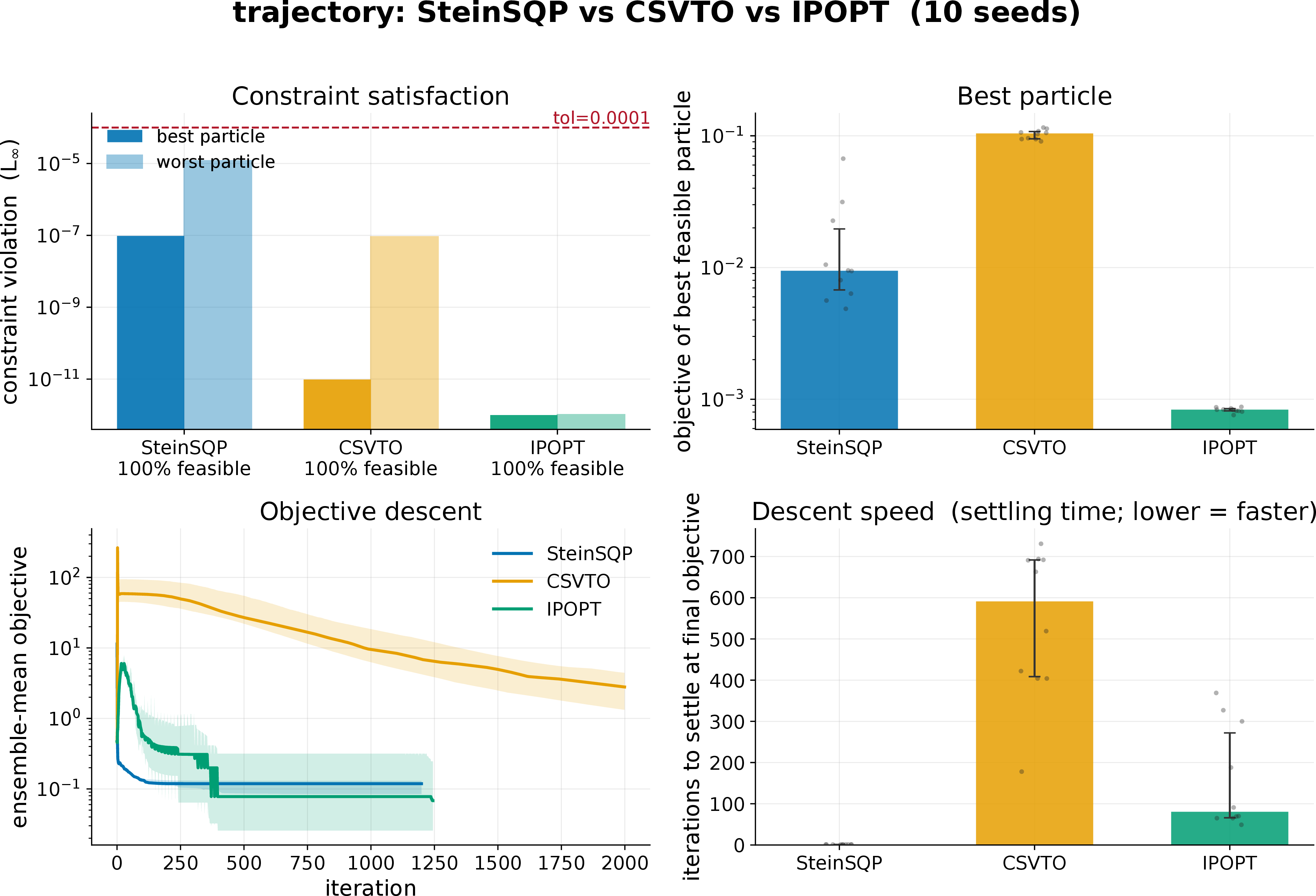

Figure 3: Convergence diagnostics on trajectory (left) and panda (right); all statistics are medians with IQR over \(10\) seeds. Per task: best- and worst-particle \(L_\infty\) violation against the task tolerance with the feasible fraction, best feasible objective, ensemble-mean objective per iteration, and the settling time, the iteration after which the mean objective stays within a \(10\%\) band of its final plateau, so oscillation counts in full..
6.1 Benchmarks, Baselines, and Protocol↩︎
Tasks. We evaluate on five tasks ordered from diagnostic to robot-scale, with the ensemble size \(N\) fixed per task. Annulus (\(N{=}88\)): sampling a 2-D Gaussian restricted to the band \(2.5\le\|x\|\le 3\); the target density is known in closed form, so distributional behavior can be judged against ground truth. Trajectory (\(N{=}16\)): planar spline trajectory optimization (33 control points) through scattered circular obstacles treated as nonlinear collision inequalities. Surface (\(N{=}32\)): traversing a curved terrain while avoiding holes; keeping the path on the terrain contributes a large system of equality constraints on top of the clearance inequalities. Panda throw (\(N{=}16\)): a 7-DoF manipulator throws a ball into a basket, under joint limits, arm and ball collision clearance, a pinned start pose, and a ballistic landing constraint (1). Push-box (\(N{=}16\)): a pusher must bring a box to a goal pose through a smoothed single-shooting contact rollout; distinct contact faces and rotation directions make the task multimodal by construction. We defer the detailed NLP problem definitions to 7.2.
Baselines. The baselines separate the two roles of the method. CSVTO, a first-order constrained Stein trajectory optimizer sharing our kernels, tests whether the second-order Stein geometry and the ensemble globalization are necessary. Multistart IPOPT, launched once from every particle of the same initial ensemble, tests whether independent deterministic solves can replace a coupled particle flow. SteinSQP and CSVTO run as batched float32 ensemble solvers on the GPU; IPOPT solves each start serially in float64 (its Python interface does not support float32), with exact sparse Lagrangian Hessians on the three low-dimensional tasks and L-BFGS on panda and push-box.
Protocol. All results aggregate \(10\) seeds per (task, method) pair. For seed \(s\) all three methods receive the identical initial ensemble, so IPOPT’s starts are bit-identical to the particle methods’ particles. Each method keeps its hand-tuned per-task configuration and runs under a shared stopping rule: a run ends as soon as all particles are feasible at the task tolerance and the ensemble merit has plateaued, with a hard cap of \(2000\) iterations. CSVTO has no globalization and never reaches this test, so it consumes the full budget on every task. IPOPT runs at KKT tolerance \(10^{-4}\), with its constraint-violation tolerance pinned to the same task feasibility tolerance the particle methods must reach. Every final ensemble is scored by one scorer: the same per-particle objective, the same \(L_\infty\) violation, and the same feasibility predicate at the true task tolerance. All timings are warm: an untimed pass first triggers XLA compilation (and compiles IPOPT’s autodiff callbacks), so the reported times measure the solve, not compilation.
6.2 Metrics↩︎
The first primary metric is particle-wise feasibility: the fraction of all returned particles, across all seeds, that satisfy the task constraints. This is the success criterion appropriate for a sampler, since a method that returns one feasible trajectory and many unusable particles has not solved the ensemble problem. The second primary metric is warm time-to-solution: for SteinSQP and CSVTO the wall time of the single batched ensemble solve, for IPOPT the sum of its \(N\) serial multistart solves. Since the Python wrapper adds callback overhead to IPOPT, we also report its callback-free internal time (wall time minus bracketed callback time) as a lower bound on a native implementation.
Secondary metrics describe sampling quality. On the annulus we report the unbiased squared maximum mean discrepancy (MMD\(^2\)) between the final ensemble and \(4000\) rejection samples of the true truncated Gaussian, using an RBF kernel with a fixed bandwidth of \(0.5\) set from the band geometry (a data-adaptive bandwidth would differ per ensemble and make the scores incomparable across methods). On push-box we report mode coverage, the number of distinct (rotation sign, contact face) labels among feasible particles, and the feasible spread, the mean pairwise distance between feasible particles. We also track the best feasible objective, the median over seeds of the lowest cost among feasible particles, as a diagnostic rather than a claim: IPOPT is expected to be strong at single-solution local optimization, while SteinSQP targets feasible, diverse ensembles.
6.3 Main Results↩︎
1 gives the headline results. SteinSQP is the only method that returns a fully feasible ensemble on every task: \(1680/1680\) particles over all seeds, against \(1504/1680\) for CSVTO and \(1599/1680\) for IPOPT. Every method finds at least one feasible particle in every seed; the gap opens at the ensemble level, which is exactly where a sampler is judged. SteinSQP also triggers the shared stopping test on every task (median \(238\)–\(1080\) of the \(2000\) allotted iterations), so its times reflect convergence, not budget exhaustion.
| Task | Method | Success | Wall time (s) | Iters. |
|---|---|---|---|---|
| Annulus (\(N{=}88\)) | SteinSQP | 100% (880/880) | 0.344 | 238 |
| CSVTO | 100% (880/880) | 0.192 | 2000\(^{\dagger}\) | |
| IPOPT | 100% (880/880) | 1.247 | 9\(^{\ddagger}\) | |
| Trajectory (\(N{=}16\)) | SteinSQP | 100% (160/160) | 0.554 | 462 |
| CSVTO | 100% (160/160) | 16.791 | 2000\(^{\dagger}\) | |
| IPOPT | 100% (160/160) | 12.679 | 146\(^{\ddagger}\) | |
| Surface (\(N{=}32\)) | SteinSQP | 100% (320/320) | 0.962 | 1080 |
| CSVTO | 100% (320/320) | 7.018 | 2000\(^{\dagger}\) | |
| IPOPT | 100% (320/320) | 4.411 | 34\(^{\ddagger}\) | |
| Panda (\(N{=}16\)) | SteinSQP | 100% (160/160) | 2.613 | 488 |
| CSVTO | 45% (72/160) | 52.789 | 2000\(^{\dagger}\) | |
| IPOPT | 99% (158/160) | 282.625 | 895\(^{\ddagger}\) | |
| Push-box (\(N{=}16\)) | SteinSQP | 100% (160/160) | 1.917 | 562 |
| CSVTO | 45% (72/160) | 3.385 | 2000\(^{\dagger}\) | |
| IPOPT | 51% (81/160) | 53.763 | 312\(^{\ddagger}\) |
Against first-order Stein (CSVTO). On the three geometric tasks CSVTO also reaches full feasibility, but because it never satisfies the stopping test it pays the full budget, ending up \(30\times\) (trajectory) and \(7\times\) (surface) slower than SteinSQP; only on the 2-D annulus, where a first-order update is nearly free, is it faster (\(0.19\) s vs.\(0.34\) s). On the two robot-scale tasks its lack of globalization becomes a correctness failure, not merely a speed one: it loses more than half the ensemble (\(45\%\) feasible on both panda and push-box), and the cost of its surviving particles degrades by up to four orders of magnitude (2). The second-order geometry and the ensemble line search are therefore not refinements; they are what makes the constrained Stein flow dependable.
Against multistart IPOPT. IPOPT matches feasibility on the smooth tasks and nearly so on panda (\(99\%\)), but as a serial multistart it is \(4.6\)–\(23\times\) slower than the batched ensemble solve there, and \(108\times\) slower on panda (\(282.6\) s vs.\(2.6\) s). This is not an artifact of wrapper overhead: even its callback-free internal lower bound (\(244.9\) s on panda, \(12.6\) s on push-box) exceeds SteinSQP’s total wall time on every task. On the contact-rich push-box rollout, interior-point iterations frequently stall, and only \(51\%\) of starts end feasible. A set of independent deterministic solves thus reproduces neither the reliability nor the cost profile of the coupled flow.
Ensemble-level convergence. 3 compares convergence from the particle-ensemble perspective. On both trajectory and panda, SteinSQP decreases the ensemble-mean objective more rapidly and reaches its final plateau earlier than the baselines, while also driving the worst-particle constraint violation below the task tolerance. This is the iteration-level convergence advantage reported in our results: the Stein–Newton flow makes faster progress per ensemble update, rather than merely obtaining a lower wall-clock time from batching. CSVTO, without globalization, exhibits larger oscillations and settles last or not within the iteration budget. IPOPT can reduce the objective quickly within individual local solves, but its progress is distributed across independent serial starts rather than a coupled ensemble update.
6.4 Sampling Quality and Diversity↩︎
| Task | SteinSQP | CSVTO | IPOPT |
|---|---|---|---|
| Annulus | \(0.500\) | \(0.530\) | \(0.500\) |
| Trajectory | \(9.46\times10^{-3}\) | \(1.04\times10^{-1}\) | \(8.33\times10^{-4}\) |
| Surface | \(325.9\) | \(473.5\) | \(310.6\) |
| Panda | \(7.53\times10^{-3}\) | \(2.39\times10^{2}\) | \(4.06\times10^{-3}\) |
| Push-box | \(6.07\times10^{-2}\) | \(1.50\times10^{-1}\) | \(1.23\times10^{-7}\) |
| Metric | SteinSQP | CSVTO | IPOPT |
|---|---|---|---|
| Annulus: MMD\(^2\) \(\downarrow\) | \(\mathbf{2.52\times10^{-3}}\) | \(9.79\times10^{-2}\) | \(6.84\times10^{-1}\) |
| Annulus: spread | \(1.32\) | \(3.48\) | \(0.00\) |
| Push-box: feasible modes \(\uparrow\) | \(2.0\) | \(2.3\) | \(2.0\) |
| Push-box: feasible spread \(\uparrow\) | \(\mathbf{3.36}\) | \(2.37\) | \(1.50\) |
3pt
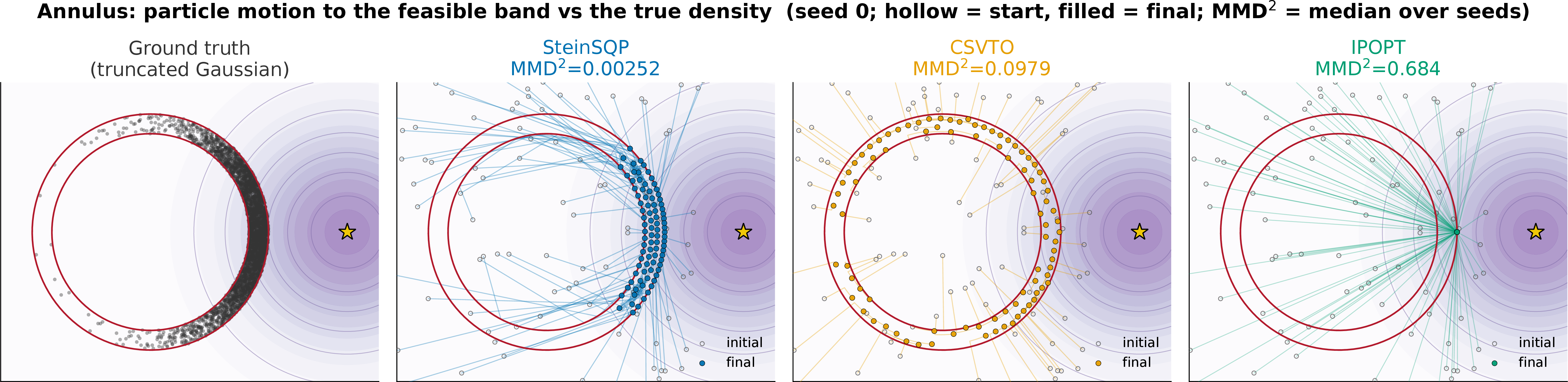
Distributional accuracy (annulus). The annulus is the one task with an exact target density, and it cleanly separates the three methods (3, 4). SteinSQP attains an MMD\(^2\) of \(2.52\times10^{-3}\), \(39\times\) lower than CSVTO and \(271\times\) lower than IPOPT. 4 shows why: all \(88\) IPOPT starts contract onto the single constrained optimum (spread \(0.00\)), so a multistart optimizer is not a sampler even when every start succeeds, while CSVTO keeps particles spread but transports them so slowly along the heavily constrained band that its ensemble never matches the target’s radial and angular profile within the budget. SteinSQP reproduces both marginals while keeping every particle in the band.
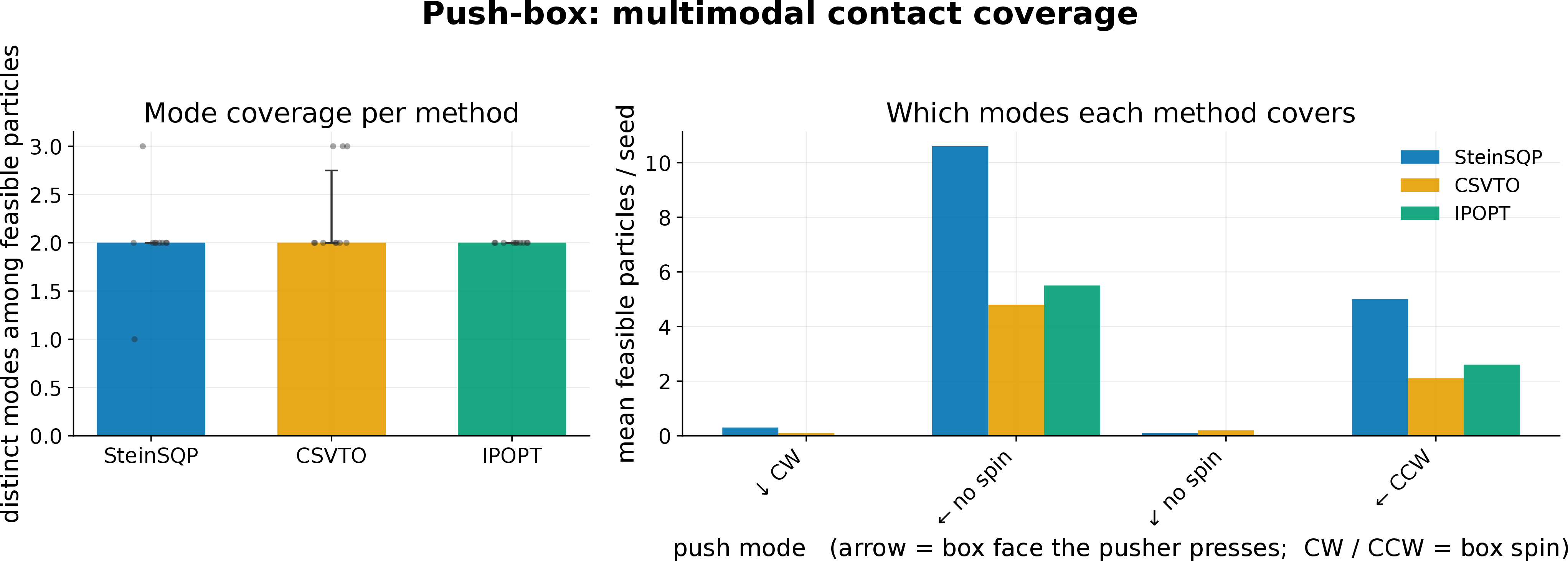
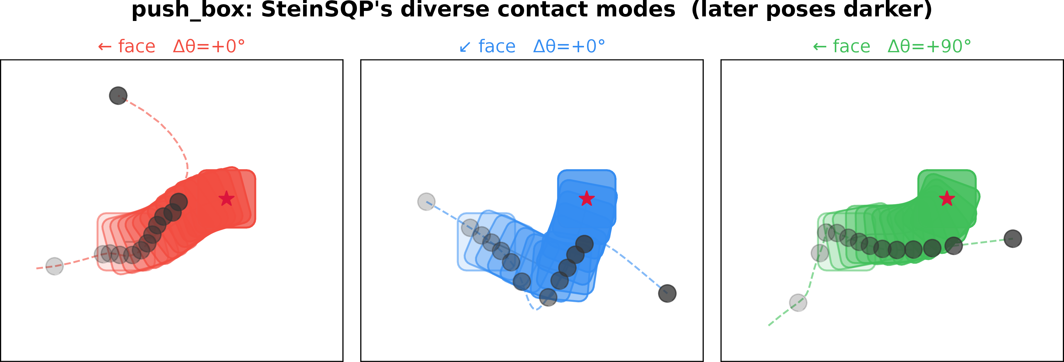
Multimodal coverage (push-box). Push-box is multimodal by construction, and here coverage must be read jointly with feasibility (3, 5). SteinSQP discovers as many feasible contact modes as multistart IPOPT (\(2.0\)) while returning \(100\%\) of its particles feasible against IPOPT’s \(51\%\), and its feasible plans are the most mutually distinct (spread \(3.36\) vs.\(2.37\) and \(1.50\)). CSVTO’s nominally highest coverage (\(2.3\)) is obtained only after discarding \(55\%\) of its ensemble. 6 renders the qualitatively different feasible pushes, opposite rotation directions and contact faces, returned by a single SteinSQP solve.
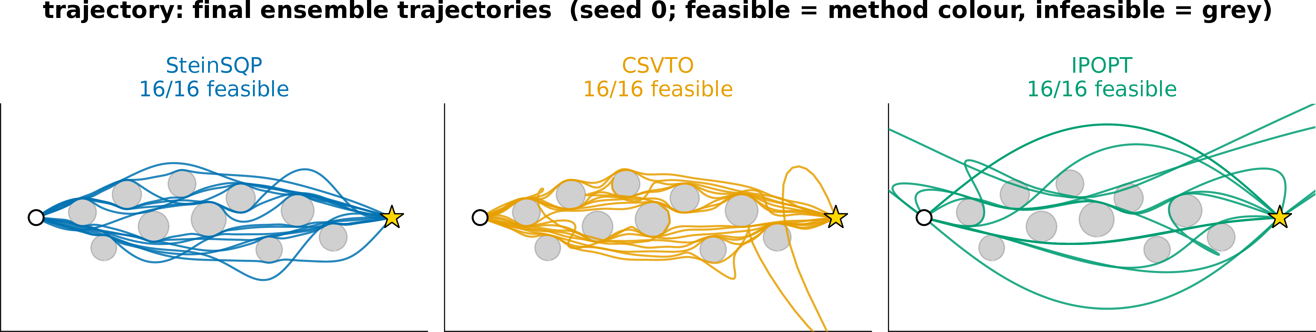
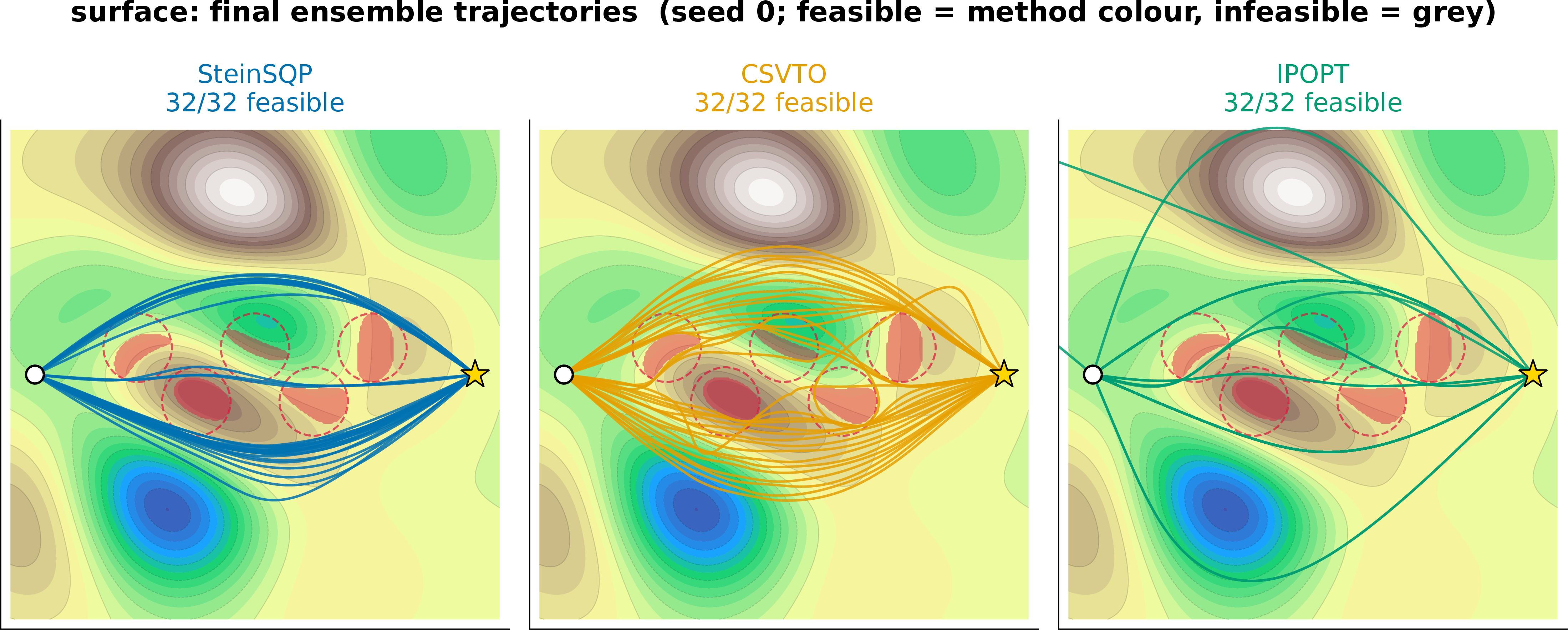
Where multistart keeps diversity. On trajectory, surface, and panda, IPOPT’s independent starts do end at distinct local optima, inheriting the spread of the shared initialization ([fig:final_traj_trajectory,fig:final_traj_surface]); on such tasks the advantage of the coupled flow is not diversity but cost, one batched solve versus a serial sum (1). The ensemble-level advantages of the flow appear precisely where the paper claims them: where the task is distributional (annulus) or contact-rich (push-box).
Best feasible cost. 2 follows the expected pattern. IPOPT, an exact float64 local optimizer, attains the lowest best-particle cost wherever it converges; SteinSQP stays close on the robot-scale tasks (within \(5\%\) on surface, the same order of magnitude on panda) while returning the entire ensemble feasible, and CSVTO’s best particle degrades by one to four orders of magnitude on the hard tasks. This is the trade the method is designed to make: a margin of best-particle optimality in exchange for a fully usable, diverse set of plans.
6.5 Takeaway↩︎
The SQP layer and the ensemble-level globalization are what make the Stein flow usable under nonlinear constraints. SteinSQP is the only method that turns the whole ensemble into feasible motion output (\(1680/1680\) particles), and it reaches that ensemble at the lowest warm time-to-solution on every task but the 2-D diagnostic, up to \(108\times\) faster than serial multistart IPOPT, whose internal solver time alone exceeds SteinSQP’s total on all five tasks. At the same time it preserves the reason to use a Stein method at all: a close match to the target distribution where one exists (\(39\)–\(271\times\) lower MMD\(^2\)) and several qualitatively distinct feasible modes in a single solve. The two baselines exhibit exactly the failure modes the method is built to remove: the first-order flow returns diverse but partially infeasible ensembles on hard constraints, and multistart nonlinear programming pays a serial cost and collapses distributionally where the task is sampling.
7 Conclusion↩︎
We presented SteinSQP, a constrained Stein variational inference method for sampling diverse feasible robot motions. Rather than relaxing nonlinear constraints through slack variables, penalties, or post-hoc projection, SteinSQP embeds linearized equality and inequality constraints directly into the kernel-coupled ensemble displacement, yielding an SQP-like constrained Stein–Newton update. A matrix-free PDHG solver makes the resulting dense kernel-space subproblem practical on GPU hardware, while an ensemble-level exact-penalty merit function globalizes the step by jointly accounting for objective decrease, nonlinear feasibility, and particle diversity.
Across five constrained motion-planning benchmarks, SteinSQP consistently produced fully feasible ensembles while retaining the diversity benefits of particle-based inference. The experiments show that this combination of curvature, direct inequality handling, and ensemble globalization is essential: first-order constrained Stein updates can remain diverse but lose feasibility on difficult robot-scale tasks, whereas independent multistart nonlinear programming can find good single solutions but pays a serial cost and may collapse distributionally. SteinSQP therefore provides a practical middle ground between constrained optimization and constrained sampling, returning a set of feasible, low-cost, and qualitatively distinct motions in a single batched solve.
Looking ahead, we aim to extend SteinSQP toward sampling-based model predictive control under strict feasibility requirements. A key direction is to study ensemble warm starts, where the feasible particle set from the previous MPC cycle is shifted forward and refined under updated state, environment, and contact constraints, potentially reusing kernel structure and SQP dual information to support real-time constrained control.
Acknowledgments↩︎
This work was supported by the DFG Emmy Noether Programme (CH 2676/1-1), the EU Horizon Europe projects MANiBOT (101120823) and ARISE (101135959), the BMFTR project RIG (16ME1001), and the ERC project SIREN (101163933). We also acknowledge support from the hessian.AI Service Center (BMFTR, 16IS22091), the hessian.AI Innovation Lab (S-DIW04/0013/003), TAM, RAI, Google, and the Alfried Krupp Foundation.
7.1 Solver Hyperparameters↩︎
Defaults shared across all experiments unless stated: damping \(\lambda=10^{-4}\) (\(10^{-3}\) on panda); ensemble line search \(K=6\), \(\beta_{\mathrm{ls}}=0.5\), \(c_1=10^{-4}\), bold-driver growth \(1.2\); exact-penalty floor \(\nu_{\min}=0.1\)–\(10\) (per example), safety \(\rho_\nu=2\); SOC damping (relative) \(10^{-3}\); PDHG \(L=24\)–\(80\) inner iterations, \(\theta=1\), safety \(0.75\)–\(0.95\), four power-iteration sweeps for the operator norm; basin-escape resampling every \(T_r=25\)–\(40\) iterations with noise \(\sigma_r=0.1\)–\(0.2\); constraint tolerance \(10^{-4}\) (\(5\times10^{-4}\) on surface; task-scale feasibility predicates on panda and push-box). The diversity temperature is the fixed \(\gamma=1\) in every experiment; the online annealing schedule (\(r_0=1\), \(r_{\min}=0.05\), \(\beta_r=0.9\)) is implemented but disabled throughout—an ablation across the examples found it is never a net win and destabilizes the stiff contact rollout. The code will be released upon official acceptance of this work.
7.2 Benchmark Problem Definitions↩︎
Every task is an instance of the constrained least-squares NLP of 3, solved jointly by an ensemble of \(N\) particles: \[\label{eq:app95nlp} \begin{align} \min_{x\in\mathbb{R}^n}\quad & V(x)=\frac{1}{2}\|r(x)\|^2,\\ \text{s.t.}\quad & h(x)=0,\qquad g(x)\le 0 . \end{align}\tag{26}\] Here a single decision vector \(x\) encodes one candidate motion. 4 lists the problem sizes. The per-task residuals, equalities, and inequalities are given below. For the spline tasks, the decision vector is the flattened control polygon \(x=\operatorname{vec}(C)\), with \(C\in\mathbb{R}^{M\times d}\), and the sampled path is the deterministic image of \(x\) under a fixed clamped cubic B-spline operator. We write \[\Delta^2 C_i = C_{i+2}-2C_{i+1}+C_i\] for the second difference of the control polygon.
| Task | \(N\) | \(n\) | \(m_h\) | \(m_g\) |
|---|---|---|---|---|
| Annulus | 88 | 2 | 0 | 2 |
| Trajectory | 16 | 66 | 4 | 1180 |
| Surface | 32 | 48 | 4 | 550 |
| Panda | 16 | 128 | 16 | 1970 |
| Push-box | 16 | 32 | 3 | 0 |
4pt
7.2.0.1 Annulus (\(n{=}2\), \(N{=}88\)).
A diagnostic sampler: each particle is a point \(x\in\mathbb{R}^2\), and the objective is the negative log-density of \(\mathcal{N}(\mu,\sigma^2 I)\), with \(\mu=(5,0)\) and \(\sigma=2\). The feasible set is the annulus \(2.5\le \|x\|\le 3\): \[\begin{align} r(x) &= \frac{x-\mu}{\sigma},\\ g_1(x) &= r_{\mathrm{in}}^2-\|x\|^2,\\ g_2(x) &= \|x\|^2-r_{\mathrm{out}}^2, \end{align}\] with \(r_{\mathrm{in}}=2.5\) and \(r_{\mathrm{out}}=3\). There are no equality constraints. The mean lies outside the band, so the unconstrained optimum is infeasible and the target is the truncated Gaussian.
7.2.0.2 Trajectory (\(n{=}66\), \(N{=}16\)).
\(M=33\) planar control points define a cubic B-spline sampled at \(S=120\) points \(p_s\). The objective penalizes control-polygon acceleration, the endpoints are pinned, and each interior sample must clear \(O=10\) disc obstacles: \[\begin{align} V(x) &= \frac{w_{\mathrm{sm}}}{2} \sum_{i=0}^{M-3}\|\Delta^2 C_i\|^2,\\ h(x) &= \bigl(C_0-x_{\mathrm{s}},\; C_{M-1}-x_{\mathrm{g}}\bigr). \end{align}\] Here \(w_{\mathrm{sm}}=1\), \(x_{\mathrm{s}}=(-5,0)\), and \(x_{\mathrm{g}}=(5,0)\). The collision inequalities are \[g_{sj}(x) = (\rho_j+\delta)^2-\|p_s-o_j\|^2 \le 0,\] for \(s=1,\ldots,S-2\) and \(j=1,\ldots,O\), with margin \(\delta=0.01\). The two endpoint samples coincide with the pinned control points and are dropped, leaving \(m_g=118\times 10\) inequalities.
7.2.0.3 Surface (\(n{=}48\), \(N{=}32\)).
\(M=24\) planar control points define a path lifted onto a smooth RBF terrain \(z=f(x,y)\), with \(P(t)=(p(t),f(p(t)))\). The objective integrates control-polygon acceleration and lifted 3-D path length by Gauss–Legendre quadrature: \[V(x) = \frac{1}{2} \int \left( w_{\mathrm{sm}}\|C''(t)\|^2 + w_{\ell}\|P'(t)\|^2 \right) \,dt .\] We use \(w_{\mathrm{sm}}=1\) and \(w_{\ell}=4\). The endpoints are pinned by \[h(x) = \bigl(C_0-x_{\mathrm{s}},\; C_{M-1}-x_{\mathrm{g}}\bigr),\] with \(x_{\mathrm{s}}=(-4.5,0)\) and \(x_{\mathrm{g}}=(4.5,0)\). The path avoids \(H=5\) spherical holes through \[g_{sj}(x) = (r_j+\delta)^2-\|P_s-b_j\|^2 \le 0,\] for \(s=1,\ldots,S\) and \(j=1,\ldots,H\), with margin \(\delta=0.05\). This gives \(m_g=110\times 5\) inequalities.
7.2.0.4 Panda throw (\(n{=}128\), \(N{=}16\)).
A \(T=16\)-knot joint trajectory with \(7\) arm joints per knot is stored in an \(8\)-wide block, giving \(x\in\mathbb{R}^{128}\) with \(112\) active variables. Let \(q_k\in\mathbb{R}^7\) be the knot configuration and \(p_k\) the forward-kinematic TCP position. The ball is released at the last knot with \[r=p_{T-1}, \qquad v=\frac{p_{T-1}-p_{T-2}}{\Delta t},\] and the flight time \(t_f\) is eliminated analytically, assuming release above the basket. The objective smooths joint acceleration: \[V(x) = \frac{1}{2} \sum_{k=0}^{T-3} \|q_{k+2}-2q_{k+1}+q_k\|^2 .\] The equality constraints enforce the start pose, zero initial velocity, and ballistic landing at the basket: \[\begin{align} h_1(x) &= q_0-q_{\mathrm{start}},\\ h_2(x) &= q_1-q_0,\\ h_3(x) &= r_{xy}+t_f v_{xy}-\mathrm{basket}_{xy}. \end{align}\] Together these give \(m_h=16\) scalar equalities. The inequalities consist of joint limits, flight-time bounds, arm–obstacle clearance, and thrown-ball clearance. Specifically, they include \(2\times7\times16=224\) joint-limit constraints, two flight-time bounds, \(16\times13\times8=1664\) arm–obstacle clearance constraints, and \(10\times8=80\) thrown-ball clearance constraints, for a total of \(m_g=1970\). All clearance constraints use margin \(m=0.03\,\mathrm{m}\); the optimizer adds a \(0.02\,\mathrm{m}\) slack.
7.2.0.5 Push-box (\(n{=}32\), \(N{=}16\)).
\(M=16\) pusher control points define a smooth pusher path over \(T=48\) rollout steps. The box pose \(\mathrm{box}_k\in SE(2)\) is not a decision variable; it is obtained by the smoothed quasi-static contact rollout \[\mathrm{box}_{k+1} = \mathrm{box}_{k} + h\,\mathrm{twist}(\mathrm{box}_{k},P_k), \qquad h=0.1,\] with \(\mathrm{box}_0=q_0=(0,0,0)\). The objective smooths the pusher control polygon: \[V(x) = \frac{w_{\mathrm{sm}}}{2} \sum_{i=0}^{M-3} \|\Delta^2 C_i\|^2, \qquad w_{\mathrm{sm}}=1 .\] The terminal box pose is pinned by \[h(x) = \left( \mathrm{box}_{T}^{xy}-\mathrm{goal},\; \sin\!\bigl(2(\theta_T-\theta_{\mathrm{goal}})\bigr) \right),\] where \(\mathrm{goal}=(1.4,0.6)\) and \(\theta_{\mathrm{goal}}=0\). There are no inequality constraints. The heading residual is \(90^\circ\)-symmetric because the rounded box is invariant under quarter turns, which admits the distinct \(\{0,\pm90^\circ\}\) rotation modes observed in 6.4.