Label-Decoupled Style Augmentation for Domain Generalization in Multi-Label Remote Sensing Scene Classification
July 14, 2026
Abstract
Multi-label classification assigns several co-occurring labels to each aerial scene, yet deployed models often encounter data distributions different from their training. Feature-statistics augmentation such as MixStyle, EFDMix, and correlated style uncertainty improves generalization at low cost but perturbs channel statistics globally, treating each image as a single style; one class can then contaminate the augmentation of another. Domain generalization is understudied for multi-label remote sensing; no prior method or multi-source benchmark targets it. A label-decoupled augmentation framework is therefore proposed, confining style perturbation to label-specific regions. Per-label attention, obtained from a learnable module or from gradient class-activation maps, yields per-label feature statistics; these statistics are mixed with cross-domain samples that share present labels, under independent per-label coefficients, and features are recomposed by attention-weighted normalization. Three operators combined with two attention sources produce six variants, evaluated on a leave-one-domain-out benchmark from multi-label UCM, AID, and DFC15 over six shared labels. Averaged over three splits and five seeds, the best variant attains 71.5% mean average precision, exceeding empirical risk minimization by 5.0 points and the strongest global-statistics baseline by 1.3 points, with the largest gain on the hardest transfer (up to 7.7 points). Ablations indicate that spatial attention and refreshed localization maps are most influential. The framework adds at most 0.35% parameters, leaves inference unchanged, and appears to offer a generic, inexpensive upgrade path for multi-label statistics-based domain generalization. Code is available upon acceptance at https://github.com/Alaa-Almouradi/Style-Augmentation-Upgrade.
Attention, domain generalization, image classification, multi-label classification, remote sensing, style augmentation.
1 Introduction↩︎
Aerial and satellite scenes rarely contain a single semantic category: a typical urban tile simultaneously exhibits buildings, vehicles, vegetation, and pavement. Multi-label classification, which assigns a set of co-occurring labels to each image, is therefore a natural formulation for remote sensing (RS) image understanding and supports applications such as land-use mapping, urban monitoring, and content-based retrieval [1]–[3]. Deep convolutional networks have become the dominant approach to this task [4]–[6], building on backbone architectures pre-trained on large-scale natural-image collections [7], [8].
These models, however, are typically trained and evaluated under the assumption of independent and identically distributed data. In practice, a classifier trained on imagery from one sensor, region, season, or ground sampling distance is frequently applied to imagery acquired under different conditions, and the resulting distribution shift degrades performance considerably [9]. Domain adaptation techniques mitigate the shift by exploiting target-domain data during training [9], [10], but such data is often unavailable before deployment. Domain generalization (DG) addresses the harder setting in which a model is trained on several source domains and must perform well on an unseen target domain [11]–[13]. Among the many DG families (invariant representation learning [14], adversarial data augmentation [15], self-supervision [16], frequency-domain augmentation [17], style-bias reduction [18], and flat-minima optimization [19]) feature-statistics augmentation has proven particularly attractive; methods such as MixStyle [20], DSU [21], EFDMix [22], and correlated style uncertainty (CSU) [23] perturb instance-level feature statistics during training, are inserted into existing backbones with a few lines of code, and add essentially no inference cost.
However, these augmentation methods share an implicit assumption that limits their suitability for multi-label imagery: they operate on global per-channel statistics, treating each image as carrying a single homogeneous style. This assumption is reasonable for object-centric, single-label benchmarks, but a multi-label RS tile is a mosaic of regions whose local statistics differ substantially; water bodies, rooftops, and vegetation produce markedly different channel responses. Mixing global statistics therefore entangles label-specific appearance. Consider a coastal tile in which ship, water, and pavement co-occur: a global statistics swap with a partner image can repaint the dark, low-variance signature of open water onto the hulls of the ships and the quay, and because a single mixing coefficient is shared by the whole image, the perturbation applied to the rare ship class is locked to that of the dominant pavement, so augmenting one class inevitably distorts the others. More generally, the style of a water region in one image may be transferred onto the building regions of another, and the coupled coefficient prevents the perturbation strength of co-occurring classes from being controlled independently. In addition, DG itself remains largely unexplored for multi-label RS classification. Recent surveys of DG in remote sensing [24] catalogue methods for single-label scene classification, object detection, change detection, and semantic segmentation, but none for multi-label scene classification, and no established multi-source evaluation benchmark exists for the latter; most multi-label RS studies evaluate within a single dataset [4], [6], [25], and cross-dataset robustness is rarely quantified in the DG setting. The present study is the first to address DG for multi-label RS scene classification and to provide a multi-source multi-label benchmark for it.
To address these limitations, this paper proposes a label-decoupled (LD) style augmentation framework that confines statistics perturbation to label-specific spatial regions. Per-label attention maps are produced either by a lightweight learnable label-localization attention module (LLAM) or by a periodically refreshed, parameter-free Grad-CAM [26] bank. These per-label attention maps decompose each feature map into per-label statistics. These statistics are then mixed exclusively between cross-domain samples that share the corresponding label, each label receiving an independent mixing coefficient, and the perturbed components are recomposed through attention-weighted normalization. The hypothesis is that confining style transfer to matching semantic regions yields more realistic style diversity and, hence, better generalization to unseen domains; this hypothesis is examined through controlled comparisons, ablations, and an analysis of the learned style manifolds. The main contributions are as follows:
A label-decoupled augmentation framework comprising attention-driven per-label statistic decomposition, cross-domain label-matched partner selection, per-label mixing coefficients, and attention-weighted recomposition. The framework is instantiated on three established operators (MixStyle [20], EFDMix [22], and CSU [23]) with two attention sources, yielding six variants. This is the first domain generalization method designed specifically for multi-label RS scene classification.
Supporting components that make the decomposition practical: a per-label cross-domain style memory bank, a global-to-per-label warm-up schedule, an attention diversity regularizer, and a label-matched domain-balanced sampler.
A leave-one-domain-out multi-label DG benchmark assembled from three public multi-label RS datasets (UCM, AID, and DFC15 [2], [3], [6], [27]–[29]) over six shared labels, which is the first multi-source multi-label domain generalization benchmark in remote sensing.
An extensive empirical study (three leave-one-domain-out splits, five seeds, eleven methods, component ablations, hyperparameter sensitivity, manifold visualization, and complexity analysis) indicating consistent improvements over the corresponding global-statistics methods at negligible cost.
The remainder of this paper is organized as follows. Section 2 reviews related work. Section 3 presents the proposed framework. Section 4 describes the benchmark and experimental setup, and Section 5 reports and discusses the results. Section 6 concludes the paper.
2 Related work↩︎
2.1 Multi-label remote sensing image classification↩︎
Multi-label learning generalizes single-label classification by allowing each sample to carry a set of labels [30], [31]. In computer vision, deep multi-label models have evolved from independent binary classifiers toward architectures that exploit label dependencies and spatial structure, e.g. recurrent label decoding [32], spatial regularization [33], and label graphs [34]. In RS, early deep approaches adapted convolutional networks to aerial multi-labeling [4], structured support vector machines incorporated spatial label correlations [25], and data augmentation was shown to benefit multi-label land-cover categorization [35]. In parallel, attention has played an increasingly central role: class-wise attention combined with recurrent modeling [3], multi-attention feature extraction [5], and attention-driven unmanned aerial vehicle (UAV) image multi-labeling [36] all localize label-relevant evidence, while relation networks [6] and graph convolutional models [37] encode inter-label dependencies. Benchmarks such as multi-label UCM [2], [27], multi-label AID [6], [28], and the DFC15 multi-label set [3], [29] have standardized within-dataset evaluation. Nevertheless, these studies almost exclusively train and test on the same distribution; the behavior of multi-label RS classifiers under domain shift has received little systematic attention in the DG setting, which motivates the benchmark used in this work.
2.2 Domain generalization↩︎
DG aims to learn, from one or several source domains, a predictor that transfers to unseen target domains without access to target data during training [11]. Comprehensive surveys categorize the field into representation-based, data-augmentation-based, and learning-strategy-based approaches [12], [13]. Representative directions include domain-invariant component analysis [14], adversarial feature alignment originally developed for adaptation [10], adversarial data augmentation [15], self-supervised auxiliary tasks [16], Fourier-based amplitude mixing [17], style-bias reduction [18], and stochastic weight averaging densely (SWAD), which seeks flat minima of the loss landscape [19].
Most of these methods are single-label by construction. Multi-label DG, in which each image carries several co-occurring labels, has received far less attention, and the few existing approaches are dominated by vision-language models, which operate on a different set of constraints. CLIPood adapts a pretrained contrastive language–image model to out-of-distribution data through a margin-based objective and a Beta-weighted parameter average [38], and Mixup-CLIPood extends this idea with a class-aware mix-up loss over larger language–image backbones [39]. Such methods inherit the broad coverage of web-scale pretraining and the multi-modal advantage, but they depend on heavy foundation backbones, are designed for generic object imagery rather than overhead scenes, and still characterize style at the image level rather than per label.
Within remote sensing, distribution shift has historically been tackled by domain adaptation, which assumes access to (typically unlabeled) target data [9]. RS DG has gained traction only recently; a dedicated survey [24] organizes RS DG methods into distribution alignment, data augmentation, and representation learning across scene classification, object detection, change detection, and semantic segmentation. Style and feature augmentation is, in fact, a recurring tool in this literature: SODA randomizes styles with adaptive instance normalization [40], FOSMix mixes style in the frequency domain for RS segmentation [41], and a style-content separation network disentangles style from content for cross-scene generalization [42]. Other lines align spectral bands across countries [43], collaborate across multiple sources [44], generalize object detectors [45], guide invariance with language [46], or fine-tune geospatial vision foundation models [47]. Crucially, every one of these methods operates on single-label scene classification, detection, change detection, segmentation, or pixel-wise hyperspectral classification; the multi-label scene-classification setting, in which several classes with distinct local styles share a single image, is addressed by none of them, and the benchmarks they adopt are correspondingly single-label [24].
These observations expose a specific gap. Global feature-statistics augmentation is cheap and effective but is single-style per image by construction; multi-label DG techniques exist but are vision-language and not tailored to overhead imagery; and RS DG, despite using style augmentation extensively, has not addressed multi-label scene classification. The framework proposed here targets precisely this intersection by decoupling style statistics per label, which is the first such treatment for multi-label RS DG.
2.3 Feature-statistics style augmentation↩︎
Instance-level feature statistics encode image style: adaptive instance normalization (AdaIN) transfers style by replacing the per-channel mean and standard deviation of one image’s features with those of another [48]. Building on this observation, MixStyle interpolates the feature statistics of random sample pairs during training [20]; DSU models statistics as Gaussian random variables and resamples them [21]; EFDMix matches higher-order statistics exactly through sorted-value interpolation [22]; and CSU perturbs statistics with channel-correlated uncertainty [23]. These methods are attractive for their simplicity, negligible cost, and strong results on single-label DG benchmarks. However, all of them compute statistics by pooling over the entire spatial extent of the feature map, which presumes one dominant style per image, and all of them draw a single mixing coefficient per image, which couples the perturbation strength of every class in the scene. Both design choices conflict with the structure of multi-label aerial imagery, in which several classes with distinct local statistics co-occur. The framework proposed in this paper removes both restrictions by decomposing statistics per label with spatial attention, obtained from a learned module or from class activation maps [26], [49], and by mixing each label’s statistics independently.
3 Proposed approach↩︎
3.1 Overview and problem formulation↩︎
Let \(\mathcal{D}_1,\dots,\mathcal{D}_S\) denote \(S\) source domains that share a label vocabulary of \(L\) classes. Each training sample is a triplet \((\mathbf{x}_i,\mathbf{y}_i,d_i)\), where \(\mathbf{x}_i\in\mathbb{R}^{3\times H_0\times W_0}\) is an image, \(\mathbf{y}_i\in\{0,1\}^{L}\) is its multi-label annotation, and \(d_i\in\{1,\dots,S\}\) is its domain index. The goal is to learn a multi-label classifier \(g:\mathbb{R}^{3\times H_0\times W_0}\to[0,1]^{L}\) that performs well on an unseen target domain.
Fig. 1 summarizes the proposed framework. A standard backbone is augmented with LD modules inserted after each layer in a set \(\mathcal{K}\) of selected layers. During training, each module (i) estimates per-label spatial attention, (ii) pools per-label feature statistics, (iii) selects a cross-domain partner that shares at least one label (or draws stored statistics from a per-label style bank), (iv) perturbs each label’s statistics independently with one of three operators, and (v) recomposes the feature map through attention-weighted normalization. The modules are stochastic and active only during training; at inference they reduce to the identity, so the deployed network is exactly the original backbone.
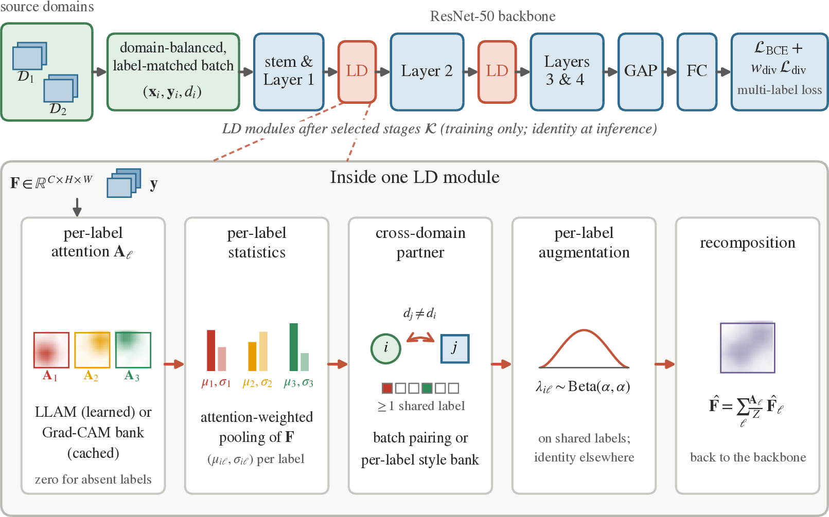
Figure 1: Overview of the proposed LD style augmentation framework. Top: training pipeline with LD modules inserted after selected backbone layers \(\mathcal{K}\); the modules are active only during training and reduce to the identity at inference. Bottom: inside one LD module, per-label attention (learned LLAM or cached Grad-CAM) yields per-label statistics, which are mixed only with cross-domain partners sharing the corresponding label (through batch pairing or a per-label style bank), perturbed with independent per-label coefficients, and recomposed by attention-weighted normalization..
3.2 Per-label decomposition and recomposition↩︎
Consider the feature map \(\mathbf{F}_i\in\mathbb{R}^{C\times H\times W}\) of sample \(i\) at an insertion point, and let \(\mathbf{A}_i\in[0,1]^{L\times H\times W}\) collect per-label attention maps (Section 3.3), with \(\mathbf{A}_{i\ell}=\mathbf{0}\) for absent labels (\(y_{i\ell}=0\)). Normalized spatial weights are obtained as \[\label{eq:attnorm} \bar{A}_{i\ell hw} \;=\; \frac{A_{i\ell hw}}{\sum_{h'=1}^{H}\sum_{w'=1}^{W} A_{i\ell h'w'} + \varepsilon},\tag{1}\] where \(\varepsilon\) is a small constant for numerical stability. The attention-weighted first and second moments of each present label \(\ell\) are \[\label{eq:stats} \begin{align} \mu_{i\ell c} &= \sum_{h,w} \bar{A}_{i\ell hw}\, F_{ichw},\\ \sigma_{i\ell c} &= \Big(\sum_{h,w} \bar{A}_{i\ell hw} F_{ichw}^{2} - \mu_{i\ell c}^{2} + \varepsilon\Big)^{\!1/2}\!, \end{align}\tag{2}\] yielding per-label style vectors \(\boldsymbol{\mu}_{i\ell},\boldsymbol{\sigma}_{i\ell}\in\mathbb{R}^{C}\). Given perturbed statistics \((\hat{\boldsymbol{\mu}}_{i\ell},\hat{\boldsymbol{\sigma}}_{i\ell})\) produced by one of the operators in Section 3.5, the augmented feature map is recomposed as a convex spatial combination of per-label stylized components, \[\label{eq:recomp} \hat{\mathbf{F}}_{i} = \sum_{\ell=1}^{L} \frac{\mathbf{A}_{i\ell}}{\mathbf{Z}_i}\odot \Big( \hat{\boldsymbol{\sigma}}_{i\ell} \frac{\mathbf{F}_{i}-\boldsymbol{\mu}_{i\ell}}{\boldsymbol{\sigma}_{i\ell}} +\hat{\boldsymbol{\mu}}_{i\ell} \Big), \quad \mathbf{Z}_i=\sum_{\ell=1}^{L}\mathbf{A}_{i\ell}+\varepsilon,\tag{3}\] where \(\odot\) denotes element-wise multiplication with broadcasting of the channel-wise statistics over spatial locations. Equation 3 performs, per label, the normalization–renormalization of AdaIN [48], but blends the results spatially according to the attention, so that each region is restyled predominantly by the statistics of the labels that occupy it. Locations not covered by any present label are dominated by the residual normalization term and remain close to the original features; labels whose statistics are left unperturbed (Section 3.4) contribute identity transformations. Each per-label branch is a channel-wise affine map of the standardized features, i.e. it preserves the spatial geometry of \(\mathbf{F}_i\) and only rescales and shifts channels; the convex, attention-weighted combination of such branches therefore yields a well-defined feature tensor that stays on the same manifold as a single AdaIN restyling, rather than an arbitrary distortion that the network could simply learn to ignore.
3.3 Per-label attention↩︎
Two interchangeable attention sources are considered.
3.3.0.1 Learned attention using LLAM
The label-localization attention module is a lightweight head consisting of two \(1\times1\) convolutions with an intermediate rectified linear unit, mapping \(\mathbf{F}_i\) to logits \(\mathbf{z}_i\in\mathbb{R}^{L\times H\times W}\), followed by a temperature-sharpened spatial softmax and masking by the ground-truth label vector: \[\label{eq:llam} A_{i\ell hw} \;=\; y_{i\ell}\, \frac{\exp\!\big(\tau\, z_{i\ell hw}\big)}{\sum_{h',w'}\exp\!\big(\tau\, z_{i\ell h'w'}\big)},\tag{4}\] where \(\tau\geq 1\) controls map sharpness. Because co-occurring labels should attend to different regions, a diversity regularizer penalizes the mean pairwise cosine similarity between the attention maps of labels that are jointly present: \[\label{eq:div} \mathcal{L}_{\mathrm{div}} =\frac{1}{B}\sum_{i=1}^{B} \frac{1}{|\mathcal{P}_i|} \sum_{(\ell,m)\in\mathcal{P}_i} \frac{\langle \mathbf{a}_{i\ell},\mathbf{a}_{im}\rangle}{\lVert\mathbf{a}_{i\ell}\rVert_2\,\lVert\mathbf{a}_{im}\rVert_2},\tag{5}\] where \(B\) is the batch size, \(\mathbf{a}_{i\ell}\in\mathbb{R}^{HW}\) is the flattened map of label \(\ell\), and \(\mathcal{P}_i=\{(\ell,m):\ell<m,\;y_{i\ell}=y_{im}=1\}\). In the configuration of Section 5, the module adds \(8.3\times10^{4}\) parameters (\(+0.35\%\)).
3.3.0.2 Cached Grad-CAM bank (GC)
As a parameter-free alternative, class activation maps [26], [49] of the network’s own predictions are used. For label \(\ell\) of sample \(i\), the map is \[\label{eq:gradcam} \begin{align} \mathbf{A}^{\mathrm{cam}}_{i\ell} &=\mathrm{ReLU}\!\Big(\sum_{c=1}^{C} w_{i\ell c}\,\mathbf{F}^{(4)}_{ic}\Big),\\ w_{i\ell c} &=\frac{1}{HW}\sum_{h,w} \frac{\partial s_{i\ell}}{\partial F^{(4)}_{ichw}}, \end{align}\tag{6}\] where \(\mathbf{F}^{(4)}_i\) is the final-stage feature map and \(s_{i\ell}\) the pre-sigmoid logit of label \(\ell\). Computing 6 online at every step would be costly and, early in training, unreliable. Instead, a bank of maps is built once the warm-up ends and is refreshed every \(R\) epochs by a single sweep over the training set; an entry is stored only if label \(\ell\) is present and currently predicted correctly, is kept in half precision on the host, and is bilinearly resized and renormalized to the resolution of each insertion point when used. Missing entries (e.g. not-yet-correct labels) fall back to the global pathway for that label. This correctness-gated caching is also what guards the decomposition against the well-known noisiness of class activation maps and their sensitivity to distribution shift: a map is admitted only where the network already localizes the label well on a source image, maps are refreshed as the model improves, and any label without a reliable entry reverts to the global operator, so a poorly localized map degrades gracefully toward the global baseline rather than injecting cross-class contamination. Because the per-label components are finally recombined by attention-weighted normalization 3 , residual localization error is further attenuated by the spatial blending. The learned LLAM source offers a complementary safeguard, as its maps are optimized end-to-end together with the mixing. The two attention sources trade off a small parameter and compute overhead with a learned, task-adaptive map (LLAM) against zero parameters with a periodic refresh cost (GC).
3.4 Cross-domain label-matched pairing and style bank↩︎
Global-statistics methods mix arbitrary sample pairs. Here, mixing partners are constrained to differ in domain and to share semantic content: sample \(i\) is paired with a partner \(j=\pi(i)\) drawn from \[\label{eq:partner} \mathcal{P}(i)=\big\{\,j:\;d_j\neq d_i\;\text{and}\; \mathbf{y}_i^{\top}\mathbf{y}_j\geq 1 \,\big\},\tag{7}\] computed within each mini-batch by a greedy matching over a domain-balanced sampler that explicitly co-locates label-compatible samples from different domains. The per-label shared mask and the effective mixing coefficient are \[\label{eq:mask} m_{i\ell}=y_{i\ell}\,y_{j\ell}, \qquad \tilde{\lambda}_{i\ell}= m_{i\ell}\,\lambda_{i\ell} + (1-m_{i\ell}),\tag{8}\] where \(\lambda_{i\ell}\sim\mathrm{Beta}(\alpha,\alpha)\), so that labels not shared with the partner receive \(\tilde{\lambda}_{i\ell}=1\), i.e. the identity, and every shared label draws an independent coefficient. For the interpolation operator, partners may alternatively be drawn from a per-label first-in-first-out style bank of size \(M\) that stores recent \((\boldsymbol{\mu}_{\cdot\ell},\boldsymbol{\sigma}_{\cdot\ell},d)\) triplets and is sampled under the same cross-domain constraint, decoupling the diversity of styles from the mini-batch composition; when a label has no cross-domain entry yet, batch pairing is used as a fallback.
3.5 Per-label augmentation operators↩︎
Three operators, illustrated in Fig. 2, instantiate the framework; each is applied per present label with the coefficient \(\tilde{\lambda}_{i\ell}\) of 8 .
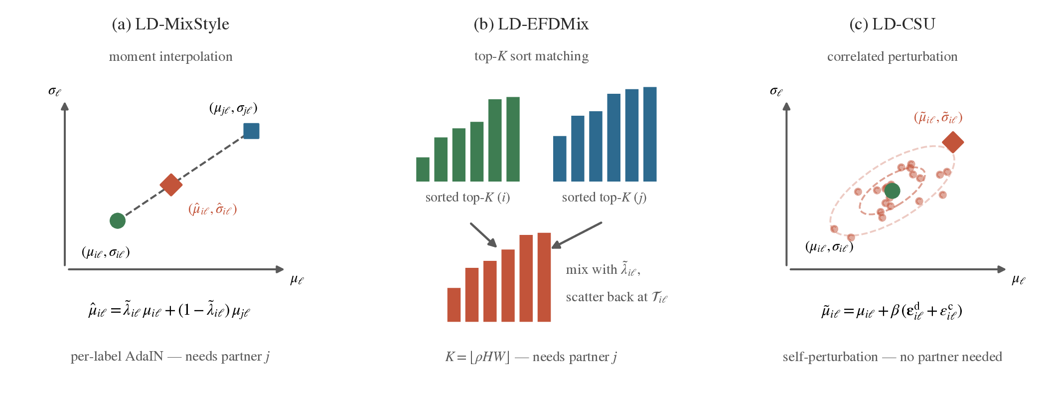
Figure 2: The three per-label augmentation operators explained in subsection 3.5. (a) LD-MixStyle interpolates the per-label moments of sample \(i\) toward those of a cross-domain partner \(j\) sharing label \(\ell\). (b) LD-EFDMix sorts the feature values at the top-\(K\) attention locations of both samples and mixes them in rank order. (c) LD-CSU perturbs the per-label moments with channel-correlated Gaussian noise and requires no partner..
3.5.0.1 LD-MixStyle
Following the interpolation principle of MixStyle [20], the perturbed statistics are convex combinations of the per-label statistics of the two samples: \[\label{eq:mixstyle} \begin{align} \hat{\boldsymbol{\mu}}_{i\ell} =\tilde{\lambda}_{i\ell}\boldsymbol{\mu}_{i\ell} +(1-\tilde{\lambda}_{i\ell})\boldsymbol{\mu}_{j\ell},\\ \quad \hat{\boldsymbol{\sigma}}_{i\ell} =\tilde{\lambda}_{i\ell}\boldsymbol{\sigma}_{i\ell} +(1-\tilde{\lambda}_{i\ell})\boldsymbol{\sigma}_{j\ell}, \end{align}\tag{9}\] These values are inserted into the recomposition 3 . The partner statistics come from the paired sample or from the style bank.
3.5.0.2 LD-EFDMix
Moment interpolation captures only first- and second-order statistics; exact feature distribution matching [22] instead operates on sorted feature values. Let \(\mathcal{T}_{i\ell}\) contain the \(K=\lfloor\rho HW\rfloor\) spatial locations with the largest attention \(A_{i\ell hw}\), and let \(\mathbf{v}^{c}_{i\ell}=\mathrm{sort}\big(\{F_{ichw}:(h,w)\in \mathcal{T}_{i\ell}\}\big)\) denote the sorted values of channel \(c\) at those locations (analogously for the partner). The mixed sequence \[\label{eq:efdmix} \hat{\mathbf{v}}^{c}_{i\ell} =\tilde{\lambda}_{i\ell}\,\mathbf{v}^{c}_{i\ell} +(1-\tilde{\lambda}_{i\ell})\,\mathbf{v}^{c}_{j\ell}\tag{10}\] is scattered back to the original locations of sample \(i\) in rank order, the partner term being treated as a constant (gradient-stopped) as in [22]; the resulting per-label value changes are then blended spatially with the attention weights, analogously to 3 . Restricting the matching to the top-\(K\) locations of both attention maps confines the exchanged distribution to label-relevant evidence.
3.5.0.3 LD-CSU
Inspired by correlated style uncertainty [23], this operator perturbs each label’s statistics without any partner. With \(\boldsymbol{\xi}\sim\mathcal{N}(\mathbf{0},\mathbf{I}_C)\) and \(\eta\sim\mathcal{N}(0,1)\), \[\label{eq:csu} \begin{align} \boldsymbol{\varepsilon}^{\mathrm{d}}_{i\ell} &=\boldsymbol{\sigma}_{i\ell}\odot\boldsymbol{\xi}, \qquad \varepsilon^{\mathrm{c}}_{i\ell} =\bar{\sigma}_{i\ell}\,\eta,\\ \tilde{\boldsymbol{\mu}}_{i\ell} &=\boldsymbol{\mu}_{i\ell} +\beta\big(\boldsymbol{\varepsilon}^{\mathrm{d}}_{i\ell} +\varepsilon^{\mathrm{c}}_{i\ell}\mathbf{1}\big),\\ \tilde{\boldsymbol{\sigma}}_{i\ell} &=\max\!\big(\boldsymbol{\sigma}_{i\ell} +\beta\,\lvert\boldsymbol{\varepsilon}^{\mathrm{d}}_{i\ell}\rvert, \varepsilon\big), \end{align}\tag{11}\] where \(\bar{\sigma}_{i\ell}\) is the channel-mean standard deviation, \(\mathbf{1}\in\mathbb{R}^{C}\) is a vector of ones, and \(\beta\) is the perturbation strength. The scalar term \(\varepsilon^{\mathrm{c}}_{i\ell}\) displaces all channels jointly, injecting the channel-correlated component advocated in [23] at the per-label level.
Combining the three operators with the two attention sources of Section 3.3 yields six variants, denoted LD-MixStyle, LD-EFDMix, LD-CSU (learned attention) and LD-MixStyle-GC, LD-EFDMix-GC, LD-CSU-GC (Grad-CAM bank).
3.6 Training procedure↩︎
Each LD module fires stochastically with probability \(p\) per batch, as in [20]. Reliable per-label attention is unavailable at the start of training: LLAM logits are untrained and network predictions, on which the Grad-CAM bank conditions, are still poor. Training therefore begins in a global mode in which the modules behave exactly like their global-statistics counterparts. For LLAM variants, the per-label pathway is blended in linearly, \[\label{eq:warmup} \begin{align} \mathbf{F}^{\mathrm{out}}_{i} &= w_e\,\hat{\mathbf{F}}^{\mathrm{LD}}_{i} +(1-w_e)\,\hat{\mathbf{F}}^{\mathrm{glob}}_{i},\\ w_e &=\min\!\big(\max\!\big((e-W)/W,\,0\big),\,1\big), \end{align}\tag{12}\] where \(e\) is the epoch index and \(W\) is the warm-up length; GC variants switch to the per-label pathway as soon as the first bank has been built after epoch \(W\). The total objective is \[\label{eq:loss} \mathcal{L} =\mathcal{L}_{\mathrm{BCE}} + w_{\mathrm{div}}\,\mathcal{L}_{\mathrm{div}},\tag{13}\] where \(\mathcal{L}_{\mathrm{BCE}}\) is the mean binary cross-entropy over labels and \(w_{\mathrm{div}}=0\) for GC variants, whose attention is not learned. At inference all modules are inactive, so the computational graph is identical to the plain backbone.
4 Experimental setup↩︎
4.1 Datasets and splits↩︎
The benchmark is assembled from three public multi-label aerial datasets whose label vocabularies overlap in six classes: building, car, tree, water, pavement, and ship. UCM [27] with the multi-label annotations of [2] contains 2100 images of \(256\times256\) pixels at approximately \(0.3\) m ground sampling distance (GSD). AID [28] with the multi-label annotations of [6] contains 3000 images of \(600\times600\) pixels collected from multiple sensors at GSDs ranging from about \(0.5\) m to \(8\) m. The DFC15 set originates from the 2015 IEEE GRSS Data Fusion Contest over Zeebrugge [29] and comprises 3342 tiles of \(600\times600\) pixels at \(0.05\) m GSD with the multi-label annotations of [3]. Vocabularies are harmonized by mapping impervious (DFC15) to pavement and boat to ship; labels outside the shared vocabulary are discarded. Table ¿tbl:tbl:datasets? summarizes the resulting per-domain statistics. The three domains differ markedly in GSD, sensor characteristics, geographic region, and label priors, e.g. tree is frequent in UCM and AID but rare in DFC15, which makes the benchmark a demanding test of multi-label generalization. Fig. 3 presents the shared classes from all domains in order to better see the variations across domains.
4.5pt
| UCM [2], [27] | AID [6], [28] | DFC15 [3], [29] | |
|---|---|---|---|
| Images | 2100 | 3000 | 3342 |
| Tile size (px) | \(256\times256\) | \(600\times600\) | \(600\times600\) |
| GSD (m) | \(\approx0.3\) | \(\approx0.5\)–\(8\) | \(0.05\) |
| Labels per image | 2.00 | 3.35 | 1.90 |
| building | 691 | 2161 | 1001 |
| car | 886 | 2026 | 705 |
| tree | 1009 | 2406 | 258 |
| water | 203 | 852 | 998 |
| pavement | 1300 | 2328 | 3133 |
| ship | 102 | 284 | 270 |
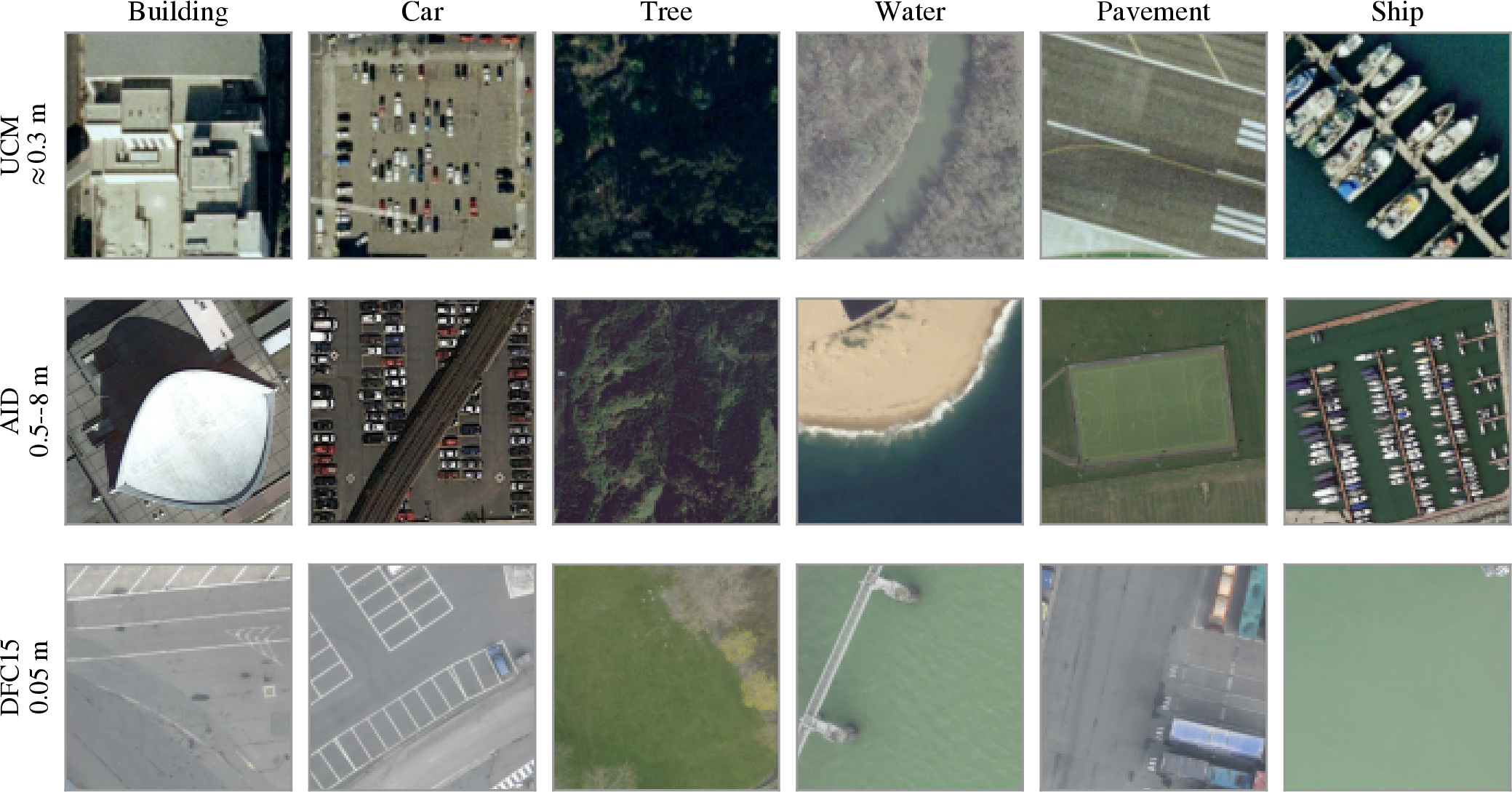
Figure 3: Class samples from each domain in the benchmark, where the domain shift can be seen through the variations between images of the same class from different domains..
Three leave-one-domain-out splits are defined: Split 1 trains on {AID, DFC15} and tests on UCM; Split 2 trains on {UCM, DFC15} and tests on AID; Split 3 trains on {UCM, AID} and tests on DFC15. Each domain is partitioned into training, validation, and test subsets (\(80/10/10\%\)) with a seed-dependent split shared by all methods; source training and validation subsets are used for learning, and the target domain is evaluated on its held-out test subset only.
4.2 Evaluation metrics↩︎
Performance is measured with threshold-free and thresholded multi-label metrics [31]: per-label average precision and its mean (mAP), the macro-averaged per-class F1 score (CF1), and the micro-averaged overall F1 score (OF1). For CF1 and OF1, a per-label decision threshold is selected on the source validation sets by maximizing the per-label F1 and is then kept fixed for target evaluation, so no target information enters threshold selection. All main results are reported as the mean and standard deviation over five seeds, which control data splits, initialization, and augmentation randomness.
4.3 Compared methods↩︎
The six LD variants are compared against empirical risk minimization (ERM) with binary cross-entropy; the three corresponding global-statistics methods: MixStyle [20], EFDMix [22], and CSU [23], all inserted at the same backbone stages; and SWAD [19] as a representative optimization-based DG method. An oracle trained and evaluated within the target domain (its training/test partitions) indicates the within-domain ceiling. All methods share the same backbone, optimizer, schedule, data augmentations, and evaluation pipeline; they differ only in the components under study.
4.4 Implementation details↩︎
All experiments use a ResNet-50 backbone [7] pre-trained on ImageNet [8], with inputs resized to \(224\times224\) pixels and augmented with horizontal/vertical flips and color jittering. Models are trained with AdamW [50] (backbone learning rate \(1.16\times10^{-4}\), classifier-head learning rate \(9.39\times10^{-4}\), weight decay \(1.59\times10^{-5}\)), a cosine schedule decaying to \(10^{-6}\), gradient-norm clipping at \(1.0\), and a batch size of \(32\) drawn by the domain-balanced label-matched sampler of Section 3.4. Training runs for at most 100 epochs with early stopping (patience 15) on the source-validation mAP. The supplementary training cost of the LD modules is analyzed in Section 5.5.
4.5 Hyperparameter selection↩︎
Hyperparameters are chosen with a leave-one-source-out (LOSO) proxy objective in the spirit of [51]: each source domain is held out in turn, the model is trained on the remaining sources, and the average held-out validation mAP constitutes the search objective. With only 2 source domains available per split, LOSO was constructed by pairing the remaining source domain with a heavily augmented version of itself as a pseudo domain. Searches are conducted with the tree-structured Parzen estimator of Optuna [52] (multivariate mode, median pruning): 40 trials for the shared optimizer parameters, reused by all methods, and 20 trials per method for the method-specific parameters listed in Table ¿tbl:tbl:search?. For some LD variants, the LOSO-selected values were further adjusted to push for more aggressive operations. Table ¿tbl:tbl:selected? lists the selected values of the headline variant.
3.5pt
| Parameter | Range | Applies to |
|---|---|---|
| backbone learning rate | \([10^{-6},5\times10^{-4}]\), log | All |
| head learning rate | \([10^{-5},5\times10^{-2}]\), log | All |
| weight decay | \([10^{-6},5\times10^{-1}]\), log | All |
| \(\alpha\) (Beta Dist.) | \(\mathcal{U}[0.1,5.0]\) | (LD-)MixStyle |
| & (LD-)EFDMix | ||
| gate probability \(p\) | \(\mathcal{U}[0.2,0.8]\) | All augmentations |
| insertion stages \(\mathcal{K}\) | subsets of \(\{1,\dots,4\}\) | LD variants |
| warm-up \(W\) (epochs) | \(\{0,\dots,10\}\) | All LD variants |
| diversity weight \(w_{\mathrm{div}}\) | \([0.01,10]\), log | LLAM variants |
| temperature \(\tau\) | \([0.1,100]\), log | LLAM variants |
| bank size \(M\) | \(\{64,128,256,512\}\) | LD-MixStyle |
| top-\(K\) ratio \(\rho\) | \(\mathcal{U}[0.01,1.0]\) | LD-EFDMix |
| strength \(\beta\) | \(\mathcal{U}[0.1,1.0]\) | (LD-)CSU |
| refresh \(R\) (epochs) | \(\{1,\dots,15\}\) | GC variants |
5pt
| Parameter | S1 | S2 | S3 |
|---|---|---|---|
| insertion stages \(\mathcal{K}\) | \(\{2\}\) | \(\{1\}\) | \(\{1\}\) |
| \(\alpha\) (Beta) | 0.45 | 5.0 | 5.0 |
| gate probability \(p\) | 0.20 | 0.80 | 0.80 |
| top-\(K\) ratio \(\rho\) | 0.34 | 0.60 | 0.60 |
| refresh \(R\) (epochs) | 9 | 13 | 13 |
| warm-up \(W\) (epochs) | 9 | 5 | 5 |
5 Results and discussion↩︎
5.1 Comparison with global-statistics augmentation↩︎
Tables ¿tbl:tbl:proto1?–¿tbl:tbl:proto3? report per-label average precision, mAP, CF1, and OF1 for the three splits, and Table ¿tbl:tbl:summary? averages the mAP results. Several observations can be discussed.
4.5pt
| Method | building | car | tree | water | pavement | ship | mAP | CF1 | OF1 |
|---|---|---|---|---|---|---|---|---|---|
| ERM (BCE) | 58.2 | 71.9 | 83.4 | 45.9 | 84.4 | 87.9 | 72.0\(\pm\)1.2 | 69.5\(\pm\)1.5 | 73.1\(\pm\)1.4 |
| MixStyle (ICLR 2021) [20] | 68.7 | 77.7 | 81.8 | 62.9 | 87.5 | 93.5 | 78.7\(\pm\)1.2 | 73.0\(\pm\)3.0 | 74.5\(\pm\)2.2 |
| EFDMix (CVPR 2022) [22] | 68.1 | 73.8 | 85.0 | 63.6 | 85.3 | 93.4 | 78.2\(\pm\)4.3 | 73.0\(\pm\)3.4 | 74.6\(\pm\)1.7 |
| CSU (WACV 2024) [23] | 70.6 | 76.6 | 83.2 | 52.2 | 85.7 | 88.3 | 76.1\(\pm\)1.5 | 71.2\(\pm\)1.0 | 73.7\(\pm\)1.8 |
| SWAD (NeurIPS 2021) [19] | 56.3 | 71.3 | 85.0 | 47.5 | 84.3 | 87.4 | 72.0\(\pm\)1.8 | 69.3\(\pm\)2.2 | 72.4\(\pm\)1.9 |
| LD-MixStyle | 67.8 | 72.4 | 85.4 | 65.3 | 84.0 | 90.4 | 77.6\(\pm\)3.6 | 73.5\(\pm\)2.6 | 74.6\(\pm\)1.9 |
| LD-EFDMix | 69.7 | 76.5 | 86.9 | 61.8 | 83.8 | 92.4 | 78.5\(\pm\)2.3 | 73.8\(\pm\)1.6 | 75.0\(\pm\)1.1 |
| LD-CSU | 67.9 | 78.4 | 85.2 | 55.2 | 85.2 | 95.2 | 77.9\(\pm\)1.8 | 73.1\(\pm\)1.2 | 74.9\(\pm\)1.9 |
| LD-MixStyle-GC | 68.0 | 74.3 | 85.6 | 61.2 | 84.4 | 96.2 | 78.3\(\pm\)2.9 | 73.7\(\pm\)2.0 | 75.0\(\pm\)2.5 |
| LD-EFDMix-GC | 71.8 | 79.0 | 84.9 | 61.0 | 83.5 | 96.6 | 79.5\(\pm\)2.4 | 74.1\(\pm\)2.4 | 74.9\(\pm\)2.2 |
| LD-CSU-GC | 69.0 | 77.3 | 85.3 | 49.4 | 85.1 | 91.9 | 76.3\(\pm\)3.3 | 72.1\(\pm\)1.9 | 74.0\(\pm\)0.8 |
| Oracle (within-domain) | 93.8 | 95.6 | 95.7 | 98.5 | 96.5 | 99.8 | 96.7\(\pm\)0.3 | 90.1\(\pm\)0.6 | 88.6\(\pm\)0.5 |
4.5pt
| Method | building | car | tree | water | pavement | ship | mAP | CF1 | OF1 |
|---|---|---|---|---|---|---|---|---|---|
| ERM (BCE) | 91.6 | 92.2 | 92.6 | 62.5 | 93.7 | 32.4 | 77.5\(\pm\)2.1 | 55.7\(\pm\)4.1 | 67.2\(\pm\)3.8 |
| MixStyle [20] | 93.0 | 92.4 | 93.6 | 61.9 | 92.3 | 27.4 | 76.8\(\pm\)1.6 | 57.3\(\pm\)1.7 | 70.8\(\pm\)1.1 |
| EFDMix [22] | 93.1 | 89.1 | 93.1 | 58.5 | 91.1 | 36.6 | 76.9\(\pm\)1.8 | 56.8\(\pm\)6.1 | 69.1\(\pm\)3.8 |
| CSU [23] | 93.1 | 92.7 | 92.8 | 63.1 | 95.6 | 32.1 | 78.2\(\pm\)1.0 | 60.2\(\pm\)2.8 | 70.1\(\pm\)2.9 |
| SWAD [19] | 91.5 | 92.6 | 92.8 | 63.5 | 93.7 | 29.9 | 77.3\(\pm\)2.1 | 54.6\(\pm\)3.8 | 66.7\(\pm\)3.9 |
| LD-MixStyle | 91.3 | 91.7 | 91.5 | 58.3 | 93.5 | 43.4 | 78.3\(\pm\)1.6 | 57.3\(\pm\)5.5 | 66.4\(\pm\)3.8 |
| LD-EFDMix | 94.5 | 92.5 | 92.5 | 61.7 | 92.6 | 40.8 | 79.1\(\pm\)1.6 | 56.0\(\pm\)2.0 | 69.1\(\pm\)1.5 |
| LD-CSU | 92.8 | 92.5 | 91.4 | 59.6 | 94.7 | 39.3 | 78.4\(\pm\)1.6 | 54.5\(\pm\)4.5 | 66.4\(\pm\)3.6 |
| LD-MixStyle-GC | 95.2 | 92.0 | 91.7 | 54.5 | 94.6 | 36.0 | 77.3\(\pm\)1.6 | 55.6\(\pm\)3.7 | 70.1\(\pm\)1.7 |
| LD-EFDMix-GC | 93.6 | 92.9 | 93.2 | 60.9 | 90.8 | 36.0 | 77.9\(\pm\)2.2 | 58.0\(\pm\)4.1 | 69.3\(\pm\)5.4 |
| LD-CSU-GC | 93.9 | 93.1 | 92.9 | 58.6 | 93.3 | 38.3 | 78.4\(\pm\)1.3 | 55.1\(\pm\)2.2 | 67.5\(\pm\)2.8 |
| Oracle (within-domain) | 99.3 | 98.3 | 98.9 | 82.5 | 99.5 | 76.5 | 92.5\(\pm\)0.4 | 86.5\(\pm\)1.5 | 92.8\(\pm\)0.8 |
4.5pt
| Method | building | car | tree | water | pavement | ship | mAP | CF1 | OF1 |
|---|---|---|---|---|---|---|---|---|---|
| ERM (BCE) | 43.1 | 42.3 | 13.5 | 62.1 | 96.1 | 43.7 | 50.1\(\pm\)6.2 | 46.2\(\pm\)4.2 | 60.4\(\pm\)2.3 |
| MixStyle [20] | 46.4 | 36.3 | 25.4 | 58.5 | 97.8 | 54.7 | 53.2\(\pm\)4.0 | 47.0\(\pm\)3.8 | 61.9\(\pm\)1.8 |
| EFDMix [22] | 48.5 | 42.8 | 17.3 | 55.9 | 98.0 | 48.8 | 51.9\(\pm\)3.8 | 46.8\(\pm\)2.0 | 63.4\(\pm\)2.1 |
| CSU [23] | 51.0 | 41.3 | 24.3 | 63.5 | 98.2 | 59.7 | 56.3\(\pm\)2.6 | 49.4\(\pm\)1.9 | 64.2\(\pm\)1.9 |
| SWAD [19] | 42.1 | 40.0 | 11.0 | 60.6 | 96.9 | 44.6 | 49.2\(\pm\)5.6 | 45.9\(\pm\)5.6 | 60.6\(\pm\)2.7 |
| LD-MixStyle | 60.0 | 48.6 | 23.4 | 61.4 | 97.4 | 52.7 | 57.3\(\pm\)3.8 | 49.4\(\pm\)3.2 | 64.0\(\pm\)1.7 |
| LD-EFDMix | 55.9 | 44.1 | 21.9 | 65.2 | 98.1 | 54.7 | 56.7\(\pm\)3.1 | 47.9\(\pm\)3.3 | 64.6\(\pm\)2.2 |
| LD-CSU | 45.3 | 47.8 | 30.7 | 69.4 | 98.2 | 55.4 | 57.8\(\pm\)2.5 | 50.9\(\pm\)2.3 | 65.9\(\pm\)2.1 |
| LD-MixStyle-GC | 51.8 | 42.8 | 17.1 | 61.3 | 98.3 | 54.0 | 54.2\(\pm\)4.3 | 49.5\(\pm\)3.1 | 65.6\(\pm\)2.5 |
| LD-EFDMix-GC | 51.7 | 52.0 | 21.9 | 61.8 | 98.4 | 57.8 | 57.3\(\pm\)5.1 | 50.8\(\pm\)3.2 | 65.5\(\pm\)1.0 |
| LD-CSU-GC | 54.2 | 43.4 | 20.4 | 66.2 | 97.8 | 57.7 | 56.6\(\pm\)2.6 | 48.3\(\pm\)2.7 | 62.7\(\pm\)2.9 |
| Oracle (within-domain) | 98.6 | 97.7 | 92.8 | 99.1 | 100.0 | 94.8 | 97.2\(\pm\)1.1 | 91.9\(\pm\)2.0 | 95.6\(\pm\)0.6 |
6pt
| Method | Average | \(\Delta\) vs.ERM |
|---|---|---|
| ERM (BCE) | 66.5 | – |
| MixStyle [20] | 69.5 | +3.0 |
| EFDMix [22] | 69.0 | +2.5 |
| CSU [23] | 70.2 | +3.7 |
| SWAD [19] | 66.2 | \(-\)0.4 |
| LD-MixStyle | 71.0 | +4.5 |
| LD-EFDMix | 71.4 | +4.9 |
| LD-CSU | 71.3 | +4.8 |
| LD-MixStyle-GC | 69.9 | +3.4 |
| LD-EFDMix-GC | 71.5 | +5.0 |
| LD-CSU-GC | 70.4 | +3.9 |
| Oracle (within-domain) | 95.4 | +28.9 |
First, statistics-based augmentation is clearly beneficial in this setting: the global methods improve the average mAP over ERM by \(2.5\)–\(3.7\) points, whereas SWAD performs on par with ERM (\(66.2\) vs. \(66.5\)), suggesting that flat-minima optimization alone does not address the dominant appearance shift between these aerial domains.
Second, label decoupling improves every operator it is applied to. With learned attention, LD-MixStyle, LD-EFDMix, and LD-CSU exceed their global counterparts by \(+1.5\), \(+2.4\), and \(+1.1\) mAP points on average, respectively; with the Grad-CAM bank, LD-EFDMix-GC gains \(+2.5\) over EFDMix and attains the best overall average of \(71.5\%\) (\(+5.0\) over ERM, \(+1.3\) over the strongest global baseline, CSU). The gains are most pronounced on Split 3, the hardest transfer (target DFC15 at \(0.05\) m GSD): ERM drops to \(50.1\%\), while LD-CSU reaches \(57.8\%\) (\(+7.7\)) and LD-EFDMix-GC and LD-MixStyle reach \(57.3\%\). The advantage of decoupling also appears at the label level: on Split 2, ERM and the global methods nearly collapse on the minority class ship (\(27\)–\(37\%\) average precision), whereas the LLAM-based LD variants recover \(39\)–\(43\%\), consistent with the premise that restricting style exchange to label-matched regions protects rare classes from being overwritten by dominant ones.
Third, the benefit of the cached attention source is operator-dependent. For EFDMix, whose sort matching directly consumes the attention-selected locations, the Grad-CAM bank is the strongest configuration on Split 1 (\(79.5\%\)) and on average; for MixStyle and CSU, the cached maps help less than the jointly trained LLAM (\(+0.4\) and \(+0.2\) average gain over the global counterparts, against \(+1.5\) and \(+1.1\) with LLAM). A plausible explanation is that moment pooling integrates over the whole map, so it benefits more from attention that is optimized end-to-end together with the mixing, whereas rank matching mainly requires that the support of the map be correct, which the Grad-CAM bank provides cheaply.
Fourth, Split 2 exhibits the smallest margins for all augmentation methods (\(76.8\)–\(79.1\%\) around an ERM of \(77.5\%\)). AID is itself a multi-sensor, multi-resolution collection [28], so its style distribution overlaps the sources more than in the other splits, leaving less room for style-based augmentation. Finally, the gap to the within-domain oracle remains large (\(13\)–\(40\) mAP points depending on the split), indicating that style augmentation alone, whether global or label-decoupled, closes only part of the domain gap; the limitation analysis in Section 5.6 returns to this point. This is expected: domain shift between these datasets is not purely a matter of style but also reflects differences in ground sampling distance, sensor and band characteristics, and class co-occurrence statistics (Table ¿tbl:tbl:datasets?), which channel-statistics operators are not designed to correct. A style-centric method is nonetheless the appropriate tool for the appearance component of the gap that the AdaIN family does model, and the manifold analysis of Section 5.4 indicates that the per-label style component is the part that aligns across domains; the residual, structural component is what the distance to the oracle reflects.
5.2 Ablation study↩︎
Table ¿tbl:tbl:ablation? removes the components of LD-EFDMix-GC one at a time on Split 1, and additionally evaluates LD-MixStyle without its style bank. Replacing the per-label attention by a uniform map (which collapses the decomposition toward global statistics) costs \(2.6\) mAP points, and freezing the Grad-CAM bank after its first construction costs \(3.3\) points, indicating that spatially correct and up-to-date localization is the core of the method. Disabling the top-\(K\) restriction (\(\rho=1\)) costs \(1.6\) points, supporting the view that sort matching should be confined to label-relevant locations. The remaining components contribute smaller but consistent amounts: per-label coefficients (\(-0.8\)), label-matched pairing (\(-0.6\)), and the warm-up (\(-0.5\)). The style bank of LD-MixStyle yields a modest \(+0.3\) over batch-only pairing, suggesting that the domain-balanced label-matched sampler already supplies sufficient cross-domain partners in this benchmark.
6pt
| Variant | mAP | CF1 | OF1 | \(\Delta\)mAP |
|---|---|---|---|---|
| LD-EFDMix-GC (full) | 79.5\(\pm\)2.4 | 74.1\(\pm\)2.4 | 74.9\(\pm\)2.2 | – |
| w/o attention (uniform map) | 76.8\(\pm\)3.0 | 72.5\(\pm\)0.8 | 74.2\(\pm\)2.3 | \(-\)2.6 |
| w/o map refresh | 76.2\(\pm\)3.5 | 72.6\(\pm\)1.2 | 74.4\(\pm\)1.3 | \(-\)3.3 |
| w/o top-\(K\) selection (\(\rho=1\)) | 77.8\(\pm\)2.9 | 71.8\(\pm\)1.1 | 73.7\(\pm\)1.3 | \(-\)1.6 |
| w/o per-label \(\lambda\) (shared \(\lambda\)) | 78.6\(\pm\)2.4 | 73.7\(\pm\)2.5 | 75.6\(\pm\)2.4 | \(-\)0.8 |
| w/o label-matched pairing | 78.8\(\pm\)1.4 | 74.1\(\pm\)2.2 | 75.1\(\pm\)2.4 | \(-\)0.6 |
| w/o warm-up | 79.0\(\pm\)2.0 | 73.2\(\pm\)1.7 | 75.5\(\pm\)1.3 | \(-\)0.5 |
| LD-MixStyle (full) | 77.6\(\pm\)3.6 | 73.5\(\pm\)2.6 | 74.6\(\pm\)1.9 | – |
| LD-MixStyle w/o style bank | 77.3\(\pm\)1.5 | 72.0\(\pm\)2.1 | 74.4\(\pm\)2.1 | \(-\)0.3 |
5.3 Hyperparameter sensitivity↩︎
Fig. 4 examines the main hyperparameters on Split 1 with single training runs at a fixed seed different from any of the main 5 seeds. The insertion point is the most influential choice: a single module after stage 2 performs best (\(83.6\%\) in this run), early-plus-deep combinations underperform, and the all-stage configuration lies in between; consistent with the common observation that style information concentrates in early-to-middle layers [20], [21]. The top-\(K\) ratio favors selective matching: the smallest tested value (\(\rho=0.2\)) performs best, and quality degrades toward \(\rho=1\), in line with the corresponding ablation. The refresh interval shows no consistent trend over \(R\in[5,15]\); the spread (\(76\)–\(82\%\)) is comparable to the seed-to-seed variability of the full model (\(\pm2.4\)), suggesting that any sufficiently frequent refresh is adequate, while never refreshing is harmful (Table ¿tbl:tbl:ablation?). The LLAM temperature exhibits a broad plateau for \(\tau\in[1,50]\) with a mild decline at \(\tau=100\), where overly sharp maps may discard context. The bank size likewise shows no consistent trend within run-to-run variability, matching its small ablation effect. Overall, apart from the insertion point, the method appears robust to its hyperparameters around the selected values.
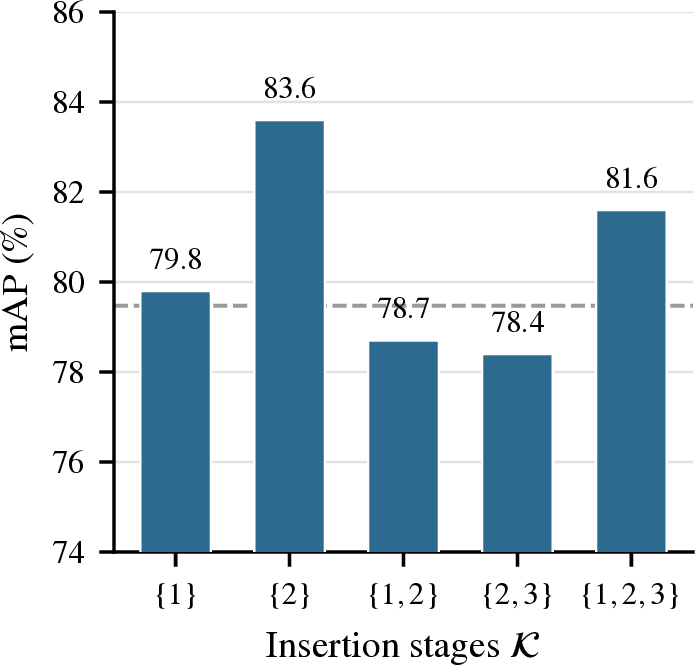
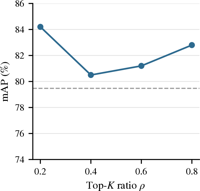
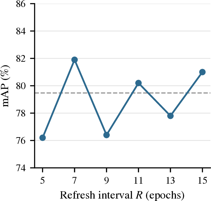
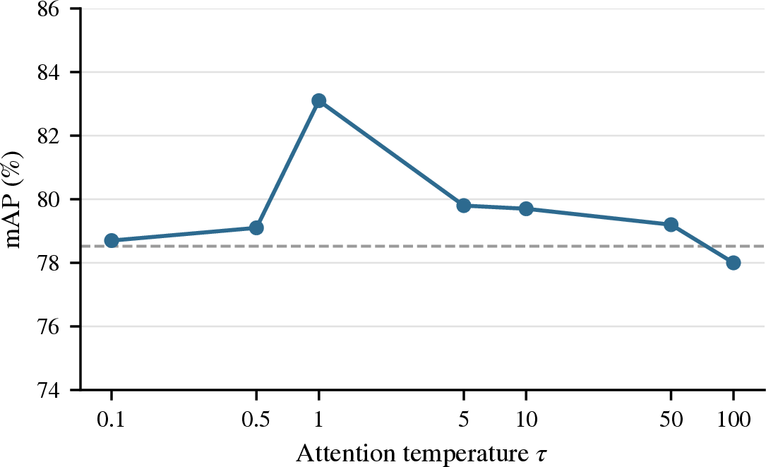
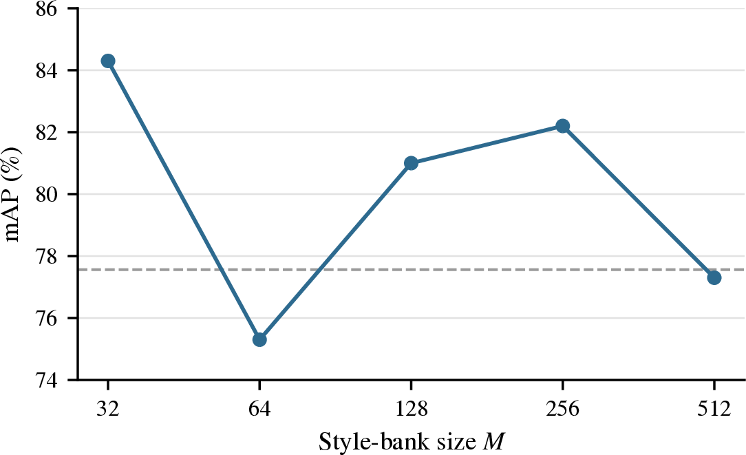
Figure 4: Hyperparameter sensitivity on Split 1 (target: UCM); each point is a single training run at a fixed seed shared by all sensitivity runs and different from any training run seed. (a)–(c) LD-EFDMix-GC: insertion stages, top-\(K\) ratio \(\rho\), and Grad-CAM refresh interval \(R\); (d) LD-EFDMix: LLAM temperature \(\tau\); (e) LD-MixStyle: style-bank size \(M\). Dashed lines show the five-seed mean of the training configuration. The refresh and top-\(K\) sweeps use a one-epoch warm-up so that the studied mechanism governs most of the run..
5.4 Style-manifold analysis↩︎
Fig. 5 visualizes, with \(t\)-SNE [53], the style statistics that the two augmentation philosophies operate on, using an LD-EFDMix model from Split 1 and the test partitions of all three domains. When global per-image statistics are embedded (Fig. 5a), points organize primarily by domain, and images carrying different labels from the same domain remain close together: the quantity that global methods mix is dominated by sensor- and scene-level appearance. The per-label statistics extracted by the proposed decomposition (Fig. 5b) instead form label-coherent groupings within which the three domain markers interleave, and target-domain points fall inside or near the groups spanned by the sources. This pattern supports the central premise of the method: per-label pooling exposes label-specific style components that are comparable across domains, which is precisely the structure that label-matched mixing exploits.
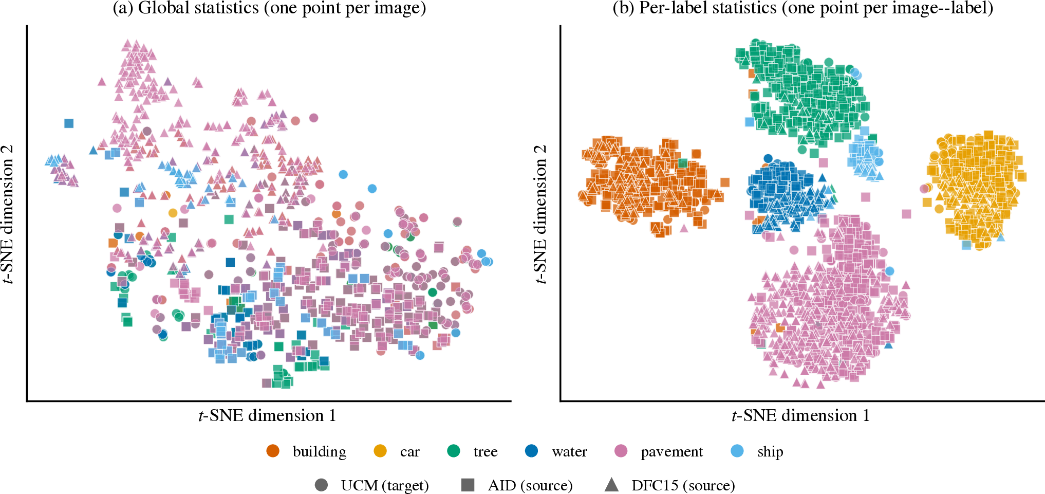
Figure 5: \(t\)-SNE [53] embeddings of style statistics for an LD-EFDMix model on Split 1 (test partitions of all domains). (a) Global per-image statistics \((\boldsymbol{\mu},\boldsymbol{\sigma})\), plotted once per (image, present label) pair for color comparability. (b) Per-label statistics \((\boldsymbol{\mu}_{\ell},\boldsymbol{\sigma}_{\ell})\) from the proposed decomposition. Colors denote labels; marker shapes denote domains..
5.5 Complexity analysis↩︎
Table ¿tbl:tbl:complexity? compares model complexity. The LLAM variants add \(8.3\times10^{4}\) parameters (\(+0.35\%\)) for the configuration with modules after stages 1 and 2; the GC variants add none. Because all modules are identities at inference, the multiply–accumulate count is unchanged (\(4.087\) G at \(224\times224\) pixels) and the measured evaluation throughput is statistically indistinguishable across methods (\(1495\)–\(1505\) images/s at batch size 32 on the GPU used in this study). Training-time overheads are confined to the augmentation pathway: LLAM adds two \(1\times1\) convolutions per inserted stage and the diversity loss, while the GC variants add approximately one extra forward–backward sweep over the training set every \(R\) epochs to rebuild the attention bank. These properties make the framework a near drop-in replacement for its global counterparts.
3pt
| Method | Params (M) | \(\Delta\) | MACs (G) | img/s |
|---|---|---|---|---|
| ERM / global | 23.52 | – | 4.087 | 1495–1498 |
| LD (LLAM) | 23.60 | \(+0.35\%\) | 4.087 | 1501–1505 |
| LD (Grad-CAM) | 23.52 | – | 4.087 | 1498–1500 |
5.6 Limitations↩︎
Several limitations should be noted. First, the gap to the within-domain oracle remains substantial (\(13\)–\(40\) mAP points), and minority classes with strong cross-domain appearance variance (ship on AID and tree on DFC15) remain difficult for every method evaluated: augmenting feature statistics cannot synthesize object scales or contexts absent from the sources. Second, gains on Split 2 are small, indicating that the benefit of style augmentation shrinks when the target’s style distribution already overlaps the sources. Third, the benchmark covers six shared labels and three domains; transfer of the conclusions to larger vocabularies and other sensor families remains to be verified due to lack of similar annotated multi-label multi-domain data in the literature. Fourth, the sensitivity study relies on single runs per configuration, so only coarse trends should be read from it. Fifth, all methods are compared under a common ResNet-50 backbone with matched training, but the study does not include large vision-language or foundation-model baselines; in general vision, multi-label DG is increasingly driven by such models (e.g. CLIPood [38] and Mixup-CLIPood [39]), and geospatial vision foundation models have begun to enter RS DG (e.g. CrossEarth [47]). A controlled comparison at that capacity is an important direction left to future work, as it entails a markedly heavier and different training and fine-tuning regime; label-decoupled statistics are, in any case, an orthogonal mechanism that could be inserted into such backbones rather than a competitor to them. Finally, the method assumes that image-level labels suffice to localize label-specific style; in scenes where a class occupies very few pixels, the attention, learned or cached, may be too coarse.
6 Conclusion↩︎
This paper introduced a label-decoupled style augmentation framework for domain generalization in multi-label remote sensing image classification. The framework replaces the global feature statistics used by MixStyle, EFDMix, and CSU with attention-derived per-label statistics, mixes them only between cross-domain samples sharing the corresponding label with independent per-label coefficients, and recomposes the feature map through attention-weighted normalization; the attention is provided either by a lightweight learned module or by a periodically refreshed Grad-CAM bank. On a leave-one-domain-out benchmark assembled from the multi-label UCM, AID, and DFC15 datasets, the proposed variants improved upon their global counterparts in all configurations, with the best variant reaching \(71.5\%\) average mAP (\(+5.0\) over ERM, and up to \(+7.7\) on the hardest transfer), at a cost of at most \(0.35\%\) additional parameters and, as for other statistics-based augmenters, no change at inference. Ablations and a manifold analysis indicate that spatially correct, up-to-date per-label localization is the decisive component, and that per-label statistics are considerably better aligned across domains than their global counterparts.
The results suggest that label decoupling is a generic and inexpensive upgrade for statistics-based augmentation whenever images contain several co-occurring classes. Future work could examine larger shared vocabularies and additional sensor families, the behavior of the decomposition on transformer backbones, the combination of label-decoupled augmentation with optimization-based methods such as weight averaging, and the integration of label-relation priors into the pairing and bank mechanisms; extending the attention sources to handle classes that occupy very few pixels is a further direction.
References↩︎
Manuscript received XX; revised XX.↩︎
This study was supported by the Scientific and Technological Research Council of Türkiye (TUBITAK) under the Grant Number 123R108.↩︎
(Corresponding author: Alaa Almouradi.)↩︎
Alaa Almouradi and Erchan Aptoula are with the Faculty of Engineering and Natural Sciences, Sabancı University, 34956 Istanbul, Türkiye (e-mail: alaaalmouradi@sabanciuniv.edu; erchan.aptoula@sabanciuniv.edu)↩︎