Learning Forced Multibody Dynamics on Lie Groups
July 14, 2026
M. D. Hansen\(^{*\dagger}\) M. Ghirardelli\(^\dagger\), E. Celledoni\(^\dagger\) , D. M. de Diego\(^\#\), B. Owren\(^\dagger\)
| \(^*\) Department of Mathematics and Cybernetics, SINTEF Digital |
| Forskningsveien 1, 0373 Oslo, Norway |
| martine.dyring.hansen@sintef.no |
| \(^\dagger\) Department of Mathematical Sciences |
| Norwegian University of Science and Technology (NTNU) |
| Alfred Getz’ vei 1, 7034 Trondheim, Norway |
| [marta.ghirardelli, elena.celledoni, brynjulf.owren]ntnu.no? |
| \(^\#\) Instituto de Ciencias Matematicas (CSIC) |
| Calle Nicolás Cabrera 13-15, Cantoblanco, 28048 Madrid, Spain |
| david.martin@icmat.es |
ABSTRACT↩︎
We propose an architecture for learning the dynamics of mechanical systems based on discrete forced Euler-Lagrange equations on Lie groups using only position data. By formulating the dynamics directly on manifold-valued configuration spaces, the method naturally respects the geometric structure of the systems and preserves geometric invariants and conservation laws. The reliance on position measurements alone makes the framework applicable in settings where velocity data are unavailable or noisy. The approach extends naturally to multibody systems, accommodates external control inputs, and demonstrates strong performance on both synthetic and real-world datasets.
1 INTRODUCTION↩︎
1.0.0.1 Motivation
Many problems in learning dynamical systems from observational data involve states evolving on nonlinear configuration spaces. In particular, rotations and rigid body motions are naturally represented by Lie groups such as \(SO(3)\), \(SE(3)\) or product manifolds thereof [1]–[8]. These representations are fundamental in a wide range of applications, including the attitude dynamics of spacecraft and drones, the pose of mobile robots, the motion of cameras and objects in computer vision, and the articulated motion of multibody systems [9]–[11]. In these settings, the available data typically consist of discrete observations that inherently satisfy geometric constraints, such as orthogonality and unit determinant. Incorporating this geometric structure into the learning process offers the opportunity to obtain models that better respect the underlying configuration manifold of the system and are more consistent with the observed data. As an example, rigid body orientations are in practice often parameterized by Euler angles. However, Euler angles provide only a local coordinate chart on \(SO(3)\): the mapping between angles and rotations is invertible only on a restricted domain and breaks down at coordinate singularities such as gimbal lock [12]. As a result, smooth rotational motions can appear discontinuous in Euler-angle coordinates, with abrupt jumps whenever the trajectory crosses a singularity. In contrast, matrix representations in \(SO(3)\) remain globally well-defined and vary smoothly along any smooth trajectory on the group.
1.0.0.2 Related works
Many existing approaches for learning dynamical systems from data assume that the state evolves in a Euclidean space. Even when modeling systems whose natural configuration manifold is a Lie group—such as rigid bodies or pendula on \(S^1\)—it is common to work in Euclidean embeddings, for example using angles, generalized coordinates, or Euclidean position-velocity representations, rather than treating \(SO(3)\) and \(SE(3)\) as configuration manifolds [13]–[16]. These approaches typically enforce physical consistency through Hamiltonian or Lagrangian formalisms, often prioritizing the preservation of symplecticity while neglecting the intrinsic geometry of the configuration manifold. In many applications, however, sensor data are already group-valued (e.g. rotation matrices or poses estimated by SLAM/visual odometry) [17]–[19]. Forcing these observations into Euclidean parametrizations can introduce coordinate singularities, discontinuities, and representation ambiguities [11]. While often effective in practice, the Euclidean assumption can be restrictive when applied to group-valued data: it can lead to violations of geometric constraints—such as loss of orthogonality or drift off the manifold—and typically requires additional projection steps or specialized parameterizations to maintain consistency with the true configuration space [1], [11], [20]–[22]. Our work is aligned with the broader effort in geometric deep learning to incorporate group and manifold structure into learning algorithms [23]–[26], but focuses specifically on mechanical systems represented by the discrete variational formulations on Lie groups, as in [27], with the flexibility to incorporate and learn external forces or controls. Our approach extends previous results on the rototranslation group [27] to more general mechanical systems, including those with external forces, multibody dynamics, and dynamics learned from real-world data.
1.0.0.3 Our contribution
In this work, we explicitly account for both the geometric and physical structure of mechanical systems. Building on the frameworks introduced in [28], [29], we develop a method for learning dynamics from data via discrete forced Euler-Lagrange equations on Lie groups [4], [30], [31]. We parameterize the discrete Lagrangian and external forces to ensure the resulting model preserves the variational structure by construction. Inspired by [29], we use the discrete Lagrangian formulation to remove the explicit dependence on velocities and recover the underlying physical structure from positions measurements only, thereby avoiding numerical differentiation of position data, which often introduces noise and complexity [32]. This stands in contrast to most Hamiltonian- and Lagrangian-based learning approaches in Euclidean spaces [13]–[15]. The resulting model operates directly on group-valued observations and represents evolution via discrete group increments, thereby avoiding Euclidean embeddings and ensuring that trajectories remain on the configuration manifold (e.g. \(SO(n)\) and \(SE(n)\)) [1], [6].
We demonstrate the proposed approach on a (controlled) rigid body evolving on \(SO(3)\) and \(SE(3)\), and real-world datasets (multibody system). Exploiting the Lie group structure guarantees that the learned states remain on the manifold, thereby eliminating the need for ad hoc projections or renormalization steps (e.g. re-orthogonalization of rotation matrices), and provides a natural representation of motion through group operations (e.g. composition of rigid motions) [7], [8]. This enables the model to encode symmetries and invariances inherent in mechanical systems [2], [6], which improves physical consistency, generalization and long-term predictive accuracy—particularly for trajectories involving large rotations, where Euclidean-based representations (e.g. Euler angles) suffer from singularities and/or discontinuities [11]. Because the architecture relies on position measurements only, it is applicable in settings where velocity data are unavailable or unreliable. Furthermore, our framework is modular: while it can identify the full dynamics (Lagrangian and forces) jointly, it also allows for the isolation and identification of specific components—such as unknown control laws—in settings where the mechanical properties of the system are already known. This is particularly relevant in robotics, for example, when learning mass matrices and friction forces from real data [32].
The paper is structured as follows. Section 2 derives the discrete forced Euler-Lagrange equations on Lie groups, which are then specialized to \(SO(3)\), \(SE(3)\) and their product manifolds in Section 3. Section 4 details the model architecture, including the loss function and regularization strategies. Finally, Section 5 presents a series of experiments validating the proposed approach.
2 DISCRETE FORCED EULER-LAGRANGE EQUATIONS ON LIE GROUPS↩︎
In this section, we first recall the continuous forced Euler-Lagrange equations on Lie groups. We then introduce discrete approximations of both the Lagrangian and the external forces and derive the corresponding discrete forced Euler-Lagrange equations on Lie groups (see [3], [6], [33]). Importantly, the resulting discretization is expressed entirely in terms of Lie group elements (positions), and does not require explicit velocities in the Lie algebra.
2.1 Trivialized forced Euler-Lagrange equations on Lie groups↩︎
Let \(Q\) be a differentiable manifold with \(\dim Q=n\) with local coordinates \((q^i)\) and \((q^i,\dot{q}^i)\) the corresponding induced coordinates on its tangent bundle \(TQ\) with canonical projection \(\tau_Q: TQ\rightarrow Q\). Denote also by \(T^*Q\) its cotangent bundle with induced coordinates \((q^i, p_i)\) and canonical projection \(\pi_Q: T^*Q\rightarrow Q\).
Given a Lagrangian function \(L\colon TQ\to{\mathbb{R}}\), and an external force \(F\colon TQ\to T^*Q\) (a fibered map over \(Q\), that is, \(\pi_Q\circ F=\tau_Q\)). The Euler-Lagrange equations for the system \((L,F)\) are \[\label{eq:EL:group:continuous} \frac{d}{dt}\left(\frac{\partial L}{\partial \dot{q}}\right) - \frac{\partial L}{\partial q} = F.\tag{1}\]
In this paper, we are interested in the case when \(Q=G\) is a Lie group. In this case, we can alternatively represent the Euler-Lagrange equations using left or right trivialization, \(TG\cong G\times\mathfrak{g}\) where \(\mathfrak{g}=T_eG\) is the Lie algebra of \(G\). Let \(g,e\in G\), \(e\) being the identity element. We denote \(\mathcal{L}_g : G \to G\) the left multiplication by \(g\), \(T_e \mathcal{L}_g : \mathfrak{g} \to T_g G\) its tangent lift at the identity, and \(\mathcal{L}_g^* : T^*_g G \to \mathfrak{g}^*\) its cotangent lift. We can then rewrite \(L\colon TG\to {\mathbb{R}}\) and \(F\colon TG\to T^*G\), using left-trivialization as \(\bar{L}\colon G\times\mathfrak{g}\to {\mathbb{R}}\) and \(\bar{F}\colon G\times\mathfrak{g}\to\mathfrak{g}^*\) by \[\bar {L}(g,\xi) = L(g, g\xi), \qquad \bar{F}(g,\xi) ={\mathcal{L}}_g^*\big(F(g,g\xi)\big),\] where \(\dot{g}=T_e {\mathcal{L}}_g\xi=g\xi\) and \(\langle {\mathcal{L}}_g^*\big(F(g,g\xi)\big), \eta\rangle=\langle F(g, g\xi), T_e{\mathcal{L}}_g (\eta)\rangle\) for \(\eta\in {\mathfrak g}\).
The left-trivialized Euler-Lagrange equations for \((\bar{L},\bar{F})\) are \[\label{eq:EL:group:} \frac{d}{dt}\left(\frac{\partial \bar{L}}{\partial \xi}\right) - \ad_{\xi}^*\left(\frac{\partial \bar{L}}{\partial \xi}\right) - {\mathcal{L}}_g^*\left(\frac{\partial \bar{L}}{\partial g}\right) = \bar{F} ,\tag{2}\] which, together with the reconstruction equation \(\dot{g}=g\xi\), are equivalent to Eq. (1 ). Here \(\ad_{\xi}^*: {\mathfrak g}^*\rightarrow {\mathfrak g}^*\) denotes the dual map of the adjoint operator \(\ad_{\xi}(\eta)=[\xi, \eta]\), where \([\; ,\;]\) is the Lie bracket of the Lie algebra \({\mathfrak g}\).
An interesting case is when the Lagrangian \(\bar{L}\) only depends on elements of \({\mathfrak g}\) (it is left-invariant), that is, \(\bar{L}(g, \xi)=l(\xi)\) for all \(g\in G\) and \(\xi\in {\mathfrak g}\). In this case, Equations (2 ) are known as the forced Euler-Poincaré equations:
\[\label{eq:ELP:group} \frac{d}{dt}\left(\frac{\partial l}{\partial \xi}\right) - \ad_{\xi}^*\left(\frac{\partial l}{\partial \xi}\right) = \bar{F} .\tag{3}\]
2.2 Discrete forced Euler-Lagrange equations on Lie groups↩︎
Since we aim at using only positions, we replace the velocity phase space \(TQ\) by \(Q\times Q\) [31]. Consider a discrete Lagrangian \(L_d: Q\times Q\rightarrow {\mathbb{R}}\) and two families of discrete external forces \(F^\pm_k\colon Q\times Q\to T^*Q\) satisfying \[F^-_k (q_k, q_{k+1})\in T^*_{q_k}Q,\qquad
F^+_k (q_k, q_{k+1})\in T^*_{q_{k+1}}Q.\] Then the discrete forced Euler-Lagrange equations are \[\label{eq:DEL} D_1 L_d(q_k,q_{k+1}) + D_2 L_d(q_{k-1},q_k) + F^-_k(q_k,q_{k+1}) +
F^+_{k-1}(q_{k-1},q_k) = 0.\tag{4}\] Given two initial points \((q_0,q_1)\), Eq. (4 ) determines iteratively \(q_{k+1}\) from the two previous points
\((q_{k-1},q_k)\) for \(k\geq 1\) under suitable regularity conditions [31].
In the particular case when \(Q\) is a Lie group \(G\), in a similar way to the continuous case, we can consider trivialized expressions. That is, instead of working with pairs \((g_k,g_{k+1})\) of consecutive points in a trajectory, we work with pairs of the form source-arrow \((g_k,W_k)\) pointing towards a target \(g_kW_k=g_{k+1}\). Hence \(W_{k}=g_{k}^{-1}g_{k+1}\). We define the “trivialized” discrete Lagrangian and forces as follows \[\begin{align} \bar{L}_d(g,W) =&
L_d(g,gW) , \qquad {\bar F}^-_k(g,W)= {\mathcal{L}}_{g}^*F^-_k(g,gW) , \qquad {\bar F}^+_k(g,W) ={\mathcal{L}}_{gW}^*F^+_k(g,gW).
\end{align}\] Observe that \(\bar{F}^-_k(g,W)\) and \({\bar F}^+_k(g,W)\) are elements of \({\mathfrak g}^*\), that is, \({\bar F}^{\pm}_k: G\times G\rightarrow {\mathfrak g}^*\).
The discrete Euler-Lagrange equations are now rewritten as \[\begin{align}
\label{eq:DEL2} {\mathcal{L}}_{g_k}^* \frac{\partial \bar{L}_d}{\partial g}(g_k, W_k) - {\mathcal{R}}_{W_k}^*\frac{\partial \bar{L}_d}{\partial W}(g_k, W_k) & + {\mathcal{L}}_{W_{k-1}}^*\frac{\partial \bar{L}_d}{\partial W}(g_{k-1}, W_{k-1}) \nonumber
\\ &+ {\bar F}^-_k (g_{k}, W_{k}) + {\bar F}^+_{k-1}(g_{k-1}, W_{k-1}) = 0,
\end{align}\tag{5}\] with the reconstruction equation \(g_{k+1}=g_kW_k\). Here, \(T{\mathcal{L}}_{g}\) and \(T{\mathcal{R}}_{g}\) are the
tangent lifts at the identity of the left and right multiplication by \(g\) in \(G\), and \({\mathcal{L}}_{g}^*\) and \({\mathcal{R}}_{g}^*\) denote the corresponding dual maps.
3 DISCRETE FORCED EULER-LAGRANGE EQUATIONS ON \(SO(3)\) AND \(SE(3)\)↩︎
In this section, we derive the previous discrete forced Euler-Lagrange equations on two specific Lie groups, \(SO(3)\) and \(SE(3)\), and use rigid body dynamics in both spaces as concrete examples. We then show how the approach generalizes to multibody systems and how control inputs can be incorporated. In all cases, the discrete approximations of the Lagrangian and the external forces are obtained using a mid-point approximation scheme.
3.1 Discrete forced Euler-Lagrange equations on \(SO(3)\).↩︎
Consider the 3D rotation group \(SO(3) = \{ R\in\mathbb{R}^{3\times 3} : R^\top R = R R^\top = I, \, \det(R) =1\}\). Its Lie algebra \(\mathfrak{so}(3)=\{\Omega \in \mathbb{R}^{3\times 3} : \Omega^\top = -\Omega \}\) can be identified with \(\mathbb{R}^3\) via the hat map \[\hat{}:\mathbb{R}^3 \to \mathfrak{so}(3),\qquad \widehat{(a,b,c)}=\begin{pmatrix} 0&-c&b\\ c&0&-a\\ -b&a&0 \end{pmatrix},\] and we let \(\vex: \mathfrak{so}(3) \to \mathbb{R}^3\) be its inverse. Consider a Lagrangian \(\bar{L} : SO(3) \times \mathfrak{so}(3) \to \mathbb{R}\), \(\bar{L} = \bar{L}(R,\omega)\). The reconstruction equation is \(\dot{R}=R\hat{\omega}\) for \(\omega \in \mathbb{R}^3\), hence \(\hat{\omega} = R^{-1} \dot{R}\) and we consider the approximation (see Moser and Veselov [34]) \[\begin{align} \hat{\omega}_k = R_k^{-1}\dot{R}_k=R_k^\top\dot{R}_k\approx R_k^\top\left( \frac{R_{k+1}-R_k}{h}\right) = \frac{R_k^\top R_{k+1}-I}{h}= \frac{W_k-I}{h}, \end{align}\] with \(W_k=R_k^{-1}R_{k+1}=R_k^\top R_{k+1} \in SO(3)\) and stepsize \(h>0\). Consider the discrete Lagrangian \(\bar{L}_d : SO(3) \times SO(3) \to \mathbb{R}\): \[\begin{align} \bar{L}_{d,k} =\bar{L}_{d} (R_k,W_k) = h \bar{L} \left(R_k, \frac{W_k - I}{h} \right). \end{align}\] Observe that in the definition of \(\bar{L}_{dk}\) we are assuming that the Lagrangian \(\bar{L}\) is defined for any \(3\times 3\)-matrix, not only on \(\mathfrak{so}(3)\). Let \(\tau_\mathrm{ext}: SO(3) \times \mathfrak{so}(3) \to \mathbb{R}^3\equiv \mathfrak{so}^*(3)\) be an external torque, a discretization is (see remark [remark:32approximation32of32log32map32in32SE3]) \[{\tau_{\mathrm{ext}}}_{d,k}^\pm = \frac{h}{2} \tau_{\mathrm{ext}} \left(R_k, \mathrm{skew} \left(\frac{W_k - I}{h} \right) \right) = \frac{h}{2} \tau_{\mathrm{ext}} \left(R_k, \frac{W_k - W_k^\top}{2h} \right).\] The discrete forced Euler-Lagrange equations 5 rewrite (see appendix 9.1 and [34]) \[\label{eq:32DEL32SO332version32with32A} A - A^\top =0\tag{6}\] where \[A:= R_k^\top \frac{\partial \bar{L}_{d,k}}{\partial R_k} - \frac{\partial \bar{L}_{d,k}}{\partial W_k} W_k + W_{k-1} \frac{\partial \bar{L}_{d,k}}{\partial W_{k-1}} + \frac{1}{2} (\widehat{{\tau_{\mathrm{ext}}}^-_{d,k}}+ \widehat{{\tau_{\mathrm{ext}}}^+_{d,k-1}}).\] Given \(R_k\) and \(W_{k-1}\), solving 6 gives \(W_k\). Then \(R_{k+1}=R_k W_k\).
The above formulation is rather general. (Some of) the derivatives in \(\eqref{eq:32DEL32SO332version32with32A}\) may be replaced by the actual derivatives if one imposes more structure on the Lagrangian, as shown in the following example. This would result in a reduction of computational cost and time, as automatic differentiation would not be needed, and in a simplification of the learning process.
Example 1 (Rigid body). Let us consider the Lagrangian of a rigid body \[\bar{L}(R,\omega) = T(\omega) - V(R) = \frac{1}{2} \omega^\top J \omega - V(R) \nonumber\] where \(J\) is the inertia matrix for vector representation. Then \[\begin{align} \bar{L}_{d,k} = \bar{L}_{d} (R_k,W_k) = \frac{1}{h}(\trace(J_d)-\trace(W_k J_d)) - h V(R_k), \end{align}\] where \(J_d\) is the inertia matrix for matrix representation satisfying \(J = \trace({J_d}) I - J_d\), as noted in [35]. Equation 6 then rewrites \[\label{eq:32discrete32EL32eq32in32SO3} - h \left( R_k^\top \frac{\partial V_{k}}{\partial R_k} - \frac{\partial V_{k}}{\partial R_k}^\top R_k \right) + \frac{1}{h} \left( J_d W_k^\top + J_d W_{k-1} \right) - \frac{1}{h} \left( W_k J_d + W_{k-1}^\top J_d \right) + (\widehat{{\tau_{\mathrm{ext}}}^-_{d,k}}+ \widehat{{\tau_{\mathrm{ext}}}^+_{d,k-1}}) = 0\qquad{(1)}\]
3.2 Discrete forced Euler-Lagrange equations on \(SE(3)\).↩︎
Consider the group of rigid transformations \(SE(3) \simeq SO(3) \times \mathbb{R}^3\) and its Lie algebra \(\mathfrak{se}(3) \simeq \mathbb{R}^3 \times \mathbb{R}^3\). For \(g\in SE(3)\) and \(\xi\in \mathfrak{se}(3)\) we have \[g=\begin{bmatrix} R & p \\ 0 & 1 \end{bmatrix}, \qquad\xi=\begin{bmatrix} \hat{\omega} & v \\ 0 & 0 \end{bmatrix}, \qquad R\in SO(3), \, \hat{\omega} \in \mathfrak{se}(3), \, p, v\in\mathbb{R}^3.\] Consider a Lagrangian \(\bar{L} : SE(3) \times \mathfrak{se}(3) \to \mathbb{R}\), \(\bar{L}=\bar{L}(R, p, \omega, v)\). The reconstruction equation is \(\Dot{g} = g\xi\), hence \(\xi = g^{-1} \Dot{g} = (R^\top \Dot{R}, R^\top \dot{p})\) and we consider the approximations \[\begin{align} \hat{\omega}_k &= R^{\top}_k \dot{R}_k \approx R_k^\top \frac{R_{k+1} - R_k}{h} = \frac{W_k - I}{h}\\ v_k &= R^{\top}_k \dot{p}_k \approx R_k^\top \frac{p_{k+1} - p_k}{h} = \frac{z_k}{h} \end{align}\] with \(W_k := R^{-1}_k R_{k+1} = R^{\top}_k R_{k+1} \in SO(3)\), \(z_k := R_k^\top (p_{k+1} - p_k) \in \mathbb{R}^3\) and stepsize \(h>0\). The discrete Lagrangian \(\bar{L}_d : SE(3) \times SE(3) \to \mathbb{R}\) is then \[\label{eq:general95discrete95lagrangian95with95potential} \bar{L}_{d,k} = \bar{L}_d (R_k, p_k, W_k, z_k) = \, h \bar{L} \left(R_k, p_k, \frac{W_k - I}{h}, \frac{z_k}{h} \right)\tag{7}\] Let \(F: SE(3) \times \mathfrak{se}(3) \to \mathbb{R}^6\equiv \mathfrak{se}^*(3)\) be an external force, and let us split \(F\) into external torque and external translational force, \(F=[\tau_\mathrm{ext}, f_\mathrm{ext}] \in \mathbb{R}^3 \times \mathbb{R}^3\). For its discretization \(( {\tau_{\mathrm{ext}}}_{d}^\pm, {f_{\mathrm{ext}}}_{d}^\pm )\), we consider the following approximation of the logarithmic map (see remark [remark:32approximation32of32log32map32in32SE3]) \[(\tilde{\omega}_k, \tilde{v}_k ) = \left( \vex \left( \mathrm{skew} \left(\frac{W_k - I}{h} \right) \right), \left( I - \frac{1}{2} h \tilde{\omega}_k \right) z_k \right) \approx \frac{\log(W_k, z_k)}{h},\] so that \[\left( {\tau_{\mathrm{ext}}}_{d,k}^\pm, {f_{\mathrm{ext}}}_{d,k}^\pm \right) = \frac{h}{2} \left( {\tau_{\mathrm{ext}}} \left(R_k, p_k, \tilde{\omega}_k, \tilde{v}_k \right), {f_{\mathrm{ext}}}\left(R_k, p_k, \tilde{\omega}_k, \tilde{v}_k \right) \right).\] The discrete forced Euler-Lagrange equation 5 rewrites (see appendix 9.2) \[\begin{align} A - A^\top & = 0 \tag{8}\\ b & = 0 \tag{9} \end{align}\] where \[\begin{align} A &:= R_k^\top \frac{\partial \bar{L}_{d,k}}{\partial R_k} - \frac{\partial \bar{L}_{d,k}}{\partial W_k} W_k^\top + \frac{1}{2} \left( \frac{\partial \bar{L}_{d,k}}{\partial z_k} \times z_k \right)^\wedge + W_{k-1}^\top \frac{\partial \bar{L}_{d,k-1}}{\partial W_{k-1}} + \frac{1}{2} (\widehat{{\tau_\mathrm{ext}}^-_{d,k}}+ \widehat{{\tau_\mathrm{ext}}^+_{d, k-1}}), \\ b &:= R_k^\top \frac{\partial \bar{L}_{d,k}}{\partial p_k} - \frac{\partial \bar{L}_{d,k}}{\partial z_{k}} + W_{k-1}^\top \frac{\partial \bar{L}_{d,k-1}}{\partial z_{k-1}} + ({f_\mathrm{ext}}^-_{d,k}+{f_\mathrm{ext}}^+_{d,k-1}). \end{align}\] Given \(R_k\), \(p_k\), \(W_{k-1}\) and \(z_{k-1}\), solving 8 9 gives \(W_k\) and \(z_k\). Then \(R_{k+1} = R_k W_k\) and \(p_{k+1} = p_k + R_k z_k\).
As in the \(SO(3)\)-case, imposing more structure on the Lagrangian may allow to replace (some of) the derivatives in 8 9 (see the rigid body example 3).
3.3 Generalization to multibody systems↩︎
The previous framework extends naturally to the product Lie group consisting of finitely many copies of \(SE(3)\) and \(SO(3)\), \[G = \underbrace{SE(3) \times\dots\times SE(3)}_m \times \underbrace{SO(3) \times\dots\times SO(3)}_n, \qquad m,n \ge 0,\] which provides an appropriate configuration space for a multibody system. An element \(g_k = (g_{1,k}, \dots, g_{m+n,k}) \in G\) encodes the states of each body at timestep \(k\), while \(\xi_k = (\xi_{1,k}, \dots, \xi_{m+n,k}) \in \mathfrak{g}\) encodes their corresponding velocities. The Lagrangian \(\bar{L}:G\times\mathfrak{g} \to \mathbb{R}\) is given by \[\bar{L}(g,\xi) = \sum_i^{m+n} \bar{L}_i(g_i,\xi_i) - V_{\mathrm{int}}(g,\xi)\] where \(\bar{L}_i(g_i,\xi_i) : SE(3) \times \mathfrak{se}(3) \to\mathbb{R}\) for \(i=1,\dots,m\), \(\bar{L}_i(g_i,\xi_i) : SO(3) \times \mathfrak{so}(3) \to\mathbb{R}\) for \(i=m+1,\dots,m+n\) are the individual Lagrangians for each body, and \(V_\mathrm{int}:G\times\mathfrak{g}\to\mathbb{R}\) is the interaction potential (e.g. a spring-damper connection, a gravitational attraction between the bodies, a penalty function representing a joint). The discrete Lagrangian \(\bar{L}_d : G \times G \to \mathbb{R}\) can be constructed as in the previous sections, along with the associated reconstruction equations and the inclusion of external forces. The discrete forced Euler-Lagrange equation 5 becomes a system of \(2m\) equations of type 8 9 and \(n\) equations of type 6 . Each body satisfies its own discrete Euler-Lagrange equation, but the equations are coupled through the partial derivatives of the interaction potential (see appendix 9.3).
3.4 Generalization to controlled systems↩︎
The external forces described in the previous sections can also be incorporated into mechanical systems actuated by control forces or control inputs (see, for instance, [2], [4], [27], [35] and references therein). Typically, these forces are described by a map \[F_c:TQ\times U\rightarrow T^*Q,\] where \(U\) denotes the set of admissible controls. Their discretization gives rise to the discrete control forces \[F_k^\pm:Q\times Q\times U\rightarrow T^*Q.\] In the Lie group setting, after left trivialization, we obtain \[\bar F_k^\pm:G\times G\times U\rightarrow\mathfrak g^*.\] The discrete controlled Euler-Lagrange equations then become \[\begin{align} \label{eq:DEL2-control} {\mathcal{L}}_{g_k}^* \frac{\partial \bar{L}_d}{\partial g}(g_k, W_k) -{\mathcal{R}}_{W_k}^* \frac{\partial \bar{L}_d}{\partial W}(g_k, W_k) +{\mathcal{L}}_{W_{k-1}}^* \frac{\partial \bar{L}_d}{\partial W}(g_{k-1}, W_{k-1}) \nonumber\\ +\,{\bar F}^-_k(g_k,W_k,u_k) +{\bar F}^+_{k-1}(g_{k-1},W_{k-1},u_{k-1}) =0, \end{align}\tag{10}\] where \(u_{k-1},u_k\in U\) are the discrete control inputs.
Example 2 (Controlled system in \(SO(3)\)). Let us consider the rigid body system in Example 1, with a control torque of the type \(\bar{\tau}_c: SO(3) \times SO(3) \times U \rightarrow {\mathbb{R}}^3\equiv \mathfrak{so}(3)^*\), \(U\subset {\mathbb{R}}^m\), given by \[\bar{\tau}_c(R, W, u)= \bar{\tau}_c( u) = C u\] where \(C\in {\mathbb{R}}^{3\times m}\). Then a simple discretization of this force is given by \[{\bar \tau^-_k}(u_k)=Cu_k\; ,\qquad {\bar \tau^+_k}(u_{k})=0\] and equation 10 rewrites \[\label{eq:DEL2-4-bis} - h \left( R_k^\top \frac{\partial V_{k}}{\partial R_k} - \frac{\partial V_{k}}{\partial R_k}^\top R_k \right) + \frac{1}{h} \left( J_d W_k^\top + J_d W_{k-1} \right) - \frac{1}{h} \left( W_k J_d + W_{k-1}^\top J_d \right) - h\widehat{Cu_k} = 0\qquad{(2)}\] with \(R_{k+1}=R_kW_k\).
4 LIE GROUP DISCRETE FORCED EULER-LAGRANGE NEURAL NETWORK (LieDFLNN)↩︎
The proposed method LieDFLNN learns the dynamics of an observed system by approximating the discrete Lagrangian and the discrete forces with neural networks \[L^\theta\approx \bar{L}_d \quad L^\theta : G\times G \to \mathbb{R}, \qquad F^\theta\approx \bar F^\pm \quad F^\theta : G\times G \to T^*G\] where \(L^\theta\) and \(F^\theta\) are parametrized by learnable parameters \(\theta\).
4.1 Loss function and regularization↩︎
4.1.0.1 Loss function.
During training, we minimize \[\label{eq:32loss32general} \mathrm{loss} = \frac{\omega_\mathrm{DEL}}{|\mathcal{T}| (N-1)} \sum_\mathcal{T} \sum_{n=1}^N \mathrm{loss}_\mathrm{DEL}(L^\theta, F^\theta) (g_{n-1}, g_n, g_{n+1}) + \frac{\omega_\mathrm{reg}}{N_R} \sum_{r=1}^{N_R} \mathrm{loss}_\mathrm{reg}(L^\theta) (g_{r}, g_{r+1}),\tag{11}\] where, \(\mathrm{loss}_\mathrm{DEL}\) is the residual of the discrete forced Euler-Lagrange equations 5 , and \(\mathrm{loss}_\mathrm{reg}\) enforces regularity of \(L^\theta\). The two terms are weighted by hyperparameters \(\omega_\mathrm{DEL}\) and \(\omega_\mathrm{reg}\), respectively. We consider a set \(\mathcal{T}\) of \(|\mathcal{T}|\) trajectories, each with \(N\) points, and use \(N_R\) pairs \((g_n, g_{n+1})\) for regularization. One may choose \(N_R=N\) and regularize over the entire dataset, but in practice we find that \(N_R<N\) is sufficient to obtain a regular Lagrangian.
The proposed framework thus learns a discrete Lagrangian and forces directly from observed trajectories by minimizing the residual of the discrete forced Euler-Lagrange equations. However, minimizing the residual alone may lead to trivial or degenerate solutions—for instance, a nearly constant Lagrangian whose derivatives vanish. The regularization term \(\mathrm{loss}_\mathrm{reg}\) is therefore crucial to ensure that the learned Lagrangian remains regular and avoid such pathological cases.
4.1.0.2 Regularity of \(L\).
A continuous Lagrangian \(L:G\times {\mathfrak g} \to \mathbb{R}\) is regular if its Hessian with respect to the left-trivialized velocity variables is non-singular at every point [35], [36]. In local coordinates, \(L\) is regular if \[\left[ \frac{\partial^2 L}{\partial \xi^i \partial \xi^j} (g,\xi) \right]_{i,j=1}^m\] is invertible for all \((g, \xi) \in TG\), where \(m\) is the dimension of the Lie group \(G\).
In our setting, \(L\) is replaced by a position-only discrete Lagrangian \(\bar{L}_d:G\times G \to \mathbb{R}\). In local coordinates, regularity of \(\bar L_d\) is defined analogously, and is equivalent to the non-singularity of the Hessian \[\mathbb{H}(\bar L_d)(g,f) = \left[ \frac{\partial^2 \bar{L}_d}{\partial g^i \partial f^j} (g, f) \right]_{i,j=1}^m\] at each \((g,f)\in G\times G\) [31], where \(f\) denotes the second configuration argument (e.g. the next configuration in time). A matrix is non-singular precisely when its determinant is nonzero, i.e. \(\det (\mathbb{H}(L^\theta)(f,g)) \ne 0\). To encourage regularity during learning, we penalize Hessians that are close to singular by enforcing that \(|\det (\mathbb{H}(L^\theta)(f,g))|\) stays above a positive threshold \(e^\epsilon\). Two possible choices of the regularizing term are: \[\mathrm{loss}_\mathrm{reg1} (L^\theta)(g,f) = \mathrm{ReLU} \left(e^\epsilon - \left|\det \left(\mathbb{H}(L^\theta)(f,g) \right) \right| \right),\] or a smooth (gaussian-type) penalty: \[\mathrm{loss}_\mathrm{reg2} (L^\theta)(g,f) = \frac{1}{e^\epsilon\sqrt{2\pi}} \exp\left( -\frac{ ( |\det(\mathbb{H}(L^\theta)(f,g))| - e^\epsilon )^2 }{2e^{2\epsilon}} \right),\] where \(\epsilon\) is a hyperparameter, and \(e^\epsilon\) sets the desired threshold away from singularity. A concrete example with detailed calculations, including a simplification for computing \(\det(\mathbb{H})\), is provided in Appendix 10.
4.2 Example (rigid body on \(SE(3)\))↩︎
Let us consider the discrete Lagrangian of a rigid body evolving on \(SE(3)\) \[\bar{L}_d(R,p,W,z) = \frac{1}{h} (\trace(J_d) - \trace(W J_d)) + \frac{1}{2h} m (z + (W - I)\rho_{\text{COM}})^\top (z + (W - I)\rho_{\text{COM}}) - h V(R, p),\] where \(J_d\) is the (symmetric positive definite) inertia matrix for matrix representation, \(m>0\) the mass and \(\rho_{COM}\in\mathbb{R}^3\) the center of mass vector in the body frame (see Example 3). Assume a linear external damping force, \(F(\omega,v) = -D \begin{pmatrix} \omega & z \end{pmatrix}^\top\) where \(D\in\mathbb{R}^{6\times 6}\) is a symmetric positive semidefinite matrix.
Our objective is to learn the discrete Lagrangian and the external forces through the components \(J_d\), \(D\), \(\rho_{COM}\) and \(V\). We parameterize each quantity by a set of trainable parameters \(\theta\), yielding \[J_d^{\theta}\in\mathbb{R}^{3 \times 3}, \qquad D^{\theta} \in \mathbb{R}^{6\times 6}, \qquad \rho_{COM}^{\theta} \in \mathbb{R}^{3}, \qquad V^{\theta}(R_k, p_k, \rho_{COM}^\theta) : \mathbb{R}^{3\times 3} \times \mathbb{R}^3 \times \mathbb{R}^3 \to \mathbb{R}.\] To ensure \(J_d^\theta\) is symmetric positive definite (SPD), we learn vectors \(r_\theta\in \mathbb{R}^3\) and \(i_\theta = (a_\theta, b_\theta, c_\theta) \in \mathbb{R}^3\), and define \[R_\theta = \exp(\widehat{r_\theta}), \qquad I_\theta = \begin{bmatrix} e^{a_\theta} + e^{b_\theta} & 0 & 0 \\ 0 & e^{a_\theta} + e^{c_\theta} & 0 \\ 0 & 0 & e^{b_\theta} + e^{c_\theta} \end{bmatrix}.\] Setting \(J_\theta = R_\theta I_\theta {R_\theta}^\top\) and \(J_d^\theta = \frac{1}{2} \trace(J_\theta) I - J_\theta\) guarantees that \(J_d^\theta\) is SPD.
To promote \(D^\theta\) being SPSD, we learn a lower triangular matrix \(L_\theta \in \mathbb{R}^{3 \times 3}\) and a vector \(\Lambda_\theta = (x_\theta,y_\theta,z_\theta) \in \mathbb{R}^3\) and set \[D^\theta = {L}_\theta {{L}_\theta}^\top + \diag({x_\theta}^2, {y_\theta}^2, {z_\theta}^2)\] The learning task is to identify \(J_d^\theta\), \(D^\theta\), \(\rho_{COM}^{\theta}\) and \(V^\theta\) such that the discrete forced Euler-Lagrange residual specified in Eq. ?? is minimized, together with the regularity penalty described above.
4.2.0.1 Rigid body in \(SO(3)\).
For a rigid body in \(SO(3)\), the discrete Lagrangian reduces to that in Example 1 The quantities we parametrize with trainable parameters are \[J_d^{\theta}\in\mathbb{R}^{3 \times 3}, \qquad D^{\theta} \in \mathbb{R}^{3\times 3}, \qquad V^{\theta}(R_k) : \mathbb{R}^{3\times 3} \to \mathbb{R},\] and we impose on \(J_d^\theta\) and \(D^\theta\) the same structure as in the \(SE(3)\) case, ensuring that they are SPD and SPSD, respectively.
4.2.0.2 Multibody systems.
In a multibody system with \(m\) bodies evolving on \(SE(3)\) and \(n\) bodies on \(SO(3)\), we write a discrete Lagrangian for each body (see Section 3.3) and learn all the components as if they were single rigid bodies in \(SE(3)\) or \(SO(3)\). To capture interactions between bodies, we additionally parameterize an interaction potential \(V_\mathrm{int}^\theta\) as a function of the configurations of all bodies.
4.2.0.3 Nonlinear external forces.
The dissipative load consider above assumes dissipation linearly proportional to the velocity, with a constant damping matrix. A more general formulation—still with linear dependence on velocity—allows the damping matrix to vary with the configuration \[F^\theta(R, p, \omega, v) = -D^\theta(R, p) \begin{pmatrix} \omega \\ v \end{pmatrix},\] where \(D^\theta(R, p) \in \mathbb{R}^{6 \times 6}\). Factorizing \(D^\theta(R,p) = L_\theta(R,p)\, L_\theta(R,p)^\top\), with \(L^\theta : SE(3) \to \mathbb{R}^{6 \times 6}\), guarantees that \(D^\theta(R, p)\) is SPSD for all configurations. This allows damping intensity and principal directions to vary with body pose, while preserving the dissipative structure.
For fully general external forces, one may use an unconstrained neural network \[F^\theta(R, p, \omega, v) = \mathrm{NN}^\theta(R, p, \omega, v) \in \mathbb{R}^6,\] which can represent any arbitrary nonlinear, non-dissipative, or energy-injecting forces (e.g. Coulomb friction, velocity-dependent inputs). The gain in expressiveness comes at the cost of the dissipative guarantee provided by the structured parameterizations above.
4.3 Inference method↩︎
After training, we perform forward prediction by integrating the learned discrete system with the discrete forced Euler-Lagrange equations. Rather than reconstructing a continuous-time model, we evolve the system directly in discrete time using the learned discrete Lagrangian and forces. In the \(SE(3)\) case, for example, given \((R_{k-1}, R_k, p_{k-1}, p_k)\) we solve the discrete forced Euler-Lagrange equations at each step for the group increments \((W_k, z_k)\) (e.g. via a root-finding method), and then update \((R_{k+1}, p_{k+1})\) accordingly. Repeating this recursion yields the predicted trajectory.
5 EXPERIMENTS↩︎
The purpose of the experiments is to evaluate the importance of (i) representing the data using a Lie group and (ii) adopting a model formulation that preserves the underlying Lie group structure such that the learned dynamics remain on the appropriate configuration manifold. We concentrate on systems evolving on \(SO(3)\) and \(SE(3)\). We investigate each component of the proposed method one at a time, comparing it with a number of different baselines.
We consider four experimental settings, each isolating one aspect of the proposed method. First, we investigate the choice of coordinates by comparing the proposed Lie group-based method with an analogous Euclidean model using Euler angles. Second, we evaluate the discrete Lie group formulation against baselines derived from the continuous forced Euler-Lagrange equations, assessing whether the discrete variational structure matters when only discrete observations are available. Third, we compare our geometry-aware approach with models that operate on matrix entries of the group elements but do not constrain predictions to the manifold, showing that the data representation alone is insufficient. Finally, we apply the proposed model to a multibody human-motion dataset on the product manifold \(SE(3) \times SO(3)^{B-1}\), focusing on a cartwheel sequence with large rotations and coordinated multibody interactions.
The code will be released upon acceptance. Architecture and training hyperparameters for every experiment are reported in Appendix 11.1 (Tables ¿tbl:tab:hyperparams-arch? and ¿tbl:tab:hyperparams-train?).
5.1 Experiment 1: Euler angles vs.matrix representation on \(SO(3)\)↩︎
Euler angles provide a compact three-dimensional parameterization of rotations but constitute only a local coordinate representation of \(SO(3)\): the map between Euler angles and rotation matrices is not globally invertible. In particular, Euler angles suffer from angle wrapping and from kinematic singularities such as gimbal lock, where one degree of freedom is lost and the remaining angles exhibit discontinuous jumps. As a result, a smooth trajectory on \(SO(3)\) may appear discontinuous when expressed in Euler angles, as illustrated in Figure 1. This forces a model trained on Euler angles to fit artificial coordinate discontinuities that are not present in the physical motion.
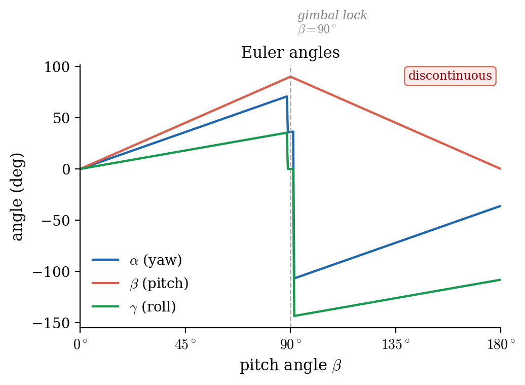
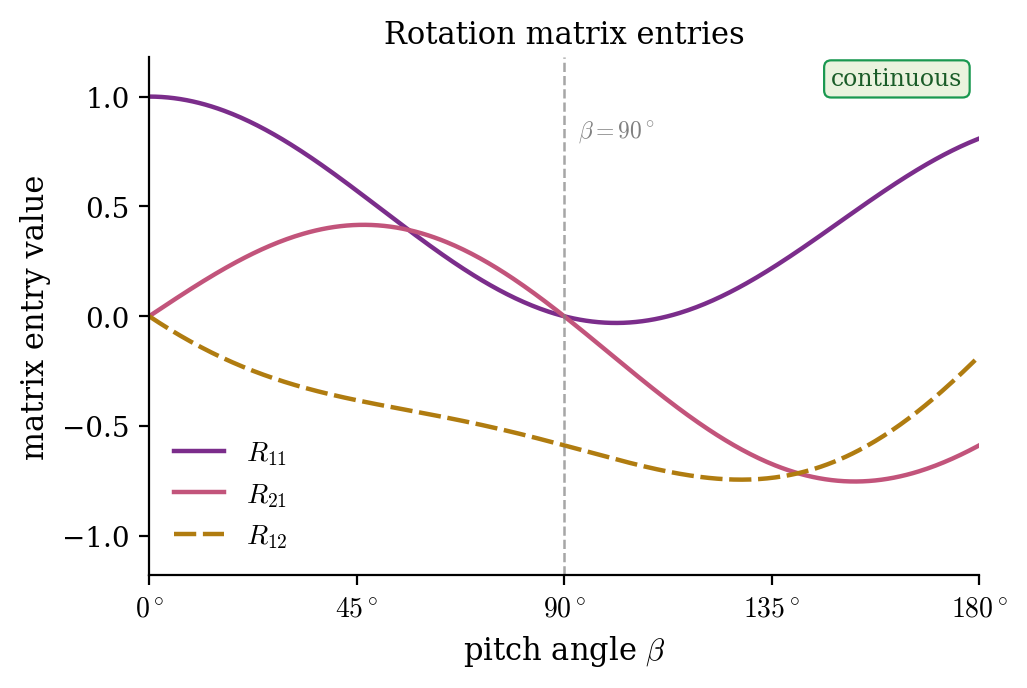
Figure 1: Discontinuity of Euler angles vs.continuity of rotation matrices. A smooth rotation trajectory (pitch \(\beta\) sweeping from \(0^\circ\) to \(180^\circ\)) is parametrized by \(ZYX\) Euler angles and rotation matrix entries . The Euler-angle representation exhibits a discontinuity at the gimbal-lock point \((\beta = 90^\circ)\), leading to abrupt jumps in \(\alpha\) and \(\gamma\). In contrast, the rotation matrix entries remain smooth throughout..
This experiment isolates the effect of the configuration-space representation. We compare the proposed LieDFLNN, which operates directly on rotation matrices \(R \in SO(3)\), against a discrete Euler-Lagrange baseline that uses Euler angles as generalized coordinates. To stress-test both representation, we systematically vary the magnitude of angular displacements, ranging from small rotations where Euler angles remain well-behaved to large rotations where singularities and wrapping artifacts are expected to degrade the baseline.
5.1.0.1 Setup and data generation.
We consider a single rigid body evolving on \(SO(3)\) subject to an external gravitational field and a frictional damping torque (see example 1 and 11.2). The governing equations are \[\begin{align} \tag{12} \dot{\omega} &= J^{-1} \left(- \omega \times (J\omega) + \tau \right), \\ \tag{13} \dot{R} &= R\hat{\omega}, \end{align}\] where \(J\in\mathbb{R}^{3\times3}\) is the symmetric positive definite inertia matrix for vector representation, and \(\tau = \tau_\mathrm{cons} + \tau_\mathrm{ext}\) is the sum of the conservative gravitational torque and the external Rayleigh dissipation torque.
Training data are generated by integrating Eq. 12 13 for \(256\) distinct initial conditions (\(R_0\), \(\omega_0\)), each over \(100\) timesteps with stepsize \(h = 0.05\), using the explicit Runge-Kutta RK45 solver
from
scipy.integrate.solve_ivp. The rigid body has mass \(m = 0.5\) and center of mass offset \(\rho_\mathrm{com} = (0,\, 0.5,\, 1.0)^\top\), and diagonal inertia tensor \(J = \mathrm{diag}(1.521,\, 1.362,\, 1.211)\), under gravitational acceleration \(g = 9.81\). The system includes linear dissipation with diagonal damping matrices \(D_{\omega\omega} = 0.1\,I\). The generated trajectories are split into a training set (\(90\%\)) and a test set (\(10\%\)).
To probe the effect of rotation magnitude in a controlled manner, all trajectories are initialized at the identity \(R_0=I\), and three datasets are produced by scaling the initial angular velocity \(\omega_0\) by factors of \(0.1\), \(0.5\) and \(0.5\). This yields motions ranging from near-identity rotations to large-angle motions that traverse regions of \(SO(3)\) where Euler-angle singularities are encountered.
The same underlying physical trajectories are represented in two ways: \[R_k \in SO(3)\] for the proposed model, and \[q_k = (\phi_k, \theta_k, \psi_k) \in \mathbb{R}^{3}\] for the baseline, where \((\phi_k, \theta_k, \psi_k)\) are ZYX Euler angles extracted from the same rotation matrices. The lie group model is trained directly on sequences \(\{R_k\}\), while the Euler-angle baseline is trained on the corresponding angle sequences.
5.1.0.2 Results and discussion.
![Figure 2: Effect of the configuration-space representation under increasing rotation magnitude (0.1\times, 0.5\times, 1.0\times initial angular velocity). [fig:euler95vs95lie95sphere]: Predicted rollouts on the unit sphere (ground truth: black). [fig:euler95vs95lie95relative-error]: Relative rotation errors, with Euler-angle predictions converted to SO(3) before evaluation to ensure a fair comparison. At small scales both methods track the true trajectory closely. As the rotation magnitude increases, the Euler-angle baseline degrades as trajectories approach singular regions, while the LieDFLNN maintains low and stable error across all scales.](/article/2607.12627/_pdflatex/zpxdyhvc.png "fig:")
Figure 2 summarizes the performance comparison. Qualitatively (Figure [fig:euler95vs95lie95sphere]), both models track the ground truth closely at the smallest scale \((0.1\times)\). However, as rotation magnitude increases, the Euler-angle baseline produces visibly inaccurate paths, while the LieDFLNN remains coincident with the ground-truth curves.
Quantitatively, Figure [fig:euler95vs95lie95relative-error] reports the relative rotation error across scales. To ensure a fair comparison, Euler-angle predictions are converted back to \(SO(3)\) before evaluation. At small magnitudes, the performance is comparable. However, at scale \((0.1\times)\), where trajectories pass through or near singular regions, the Euler-angle baseline degrades substantially due to the coordinate discontinuities shown in Figure 1 (a). In contrast, the LieDFLNN maintains consistently low error across all scales, as rotation matrices remain smooth and non-singular everywhere on the manifold.
5.2 Experiment 2: Discrete vs.continuous Euler-Lagrange equations on \(SO(3)\)↩︎
While a continuous-time forced Euler-Lagrange framework can be formulated on \(SO(3)\), its implementation faces two practical challenges. First, integrating a learned continuous vector field with generic solvers does not guarantee that the trajectory remains on the Lie group, leading to geometric drift. Second, because training data consist of discrete observations, continuous models require recovering velocities through finite differences, introducing approximation errors before training even begins.
This experiment compares our discrete Lie group formulation against continuous-time Euler-Lagrange baselines that share the same \(SO(3)\) structure but differ in their integration schemes. By varying the training trajectory length, we investigate whether the discrete formulation offers superior accuracy and robustness when learning from limited temporal context.
5.2.0.1 Setup and data generation.
We train and evaluate on a single rigid body evolving on \(SO(3)\) subject to an external torque \(\tau\). The governing equations are 12 13 as in Experiment 1, but here \(\tau\) has no gravitational component and consists only of the external torque (see Appendix 11.2).
The training dataset consists of \(128\) trajectories, each generated from a random initial configuration \((R_0, \omega_0)\) and integrated for \(100\)
timesteps with stepsize \(h = 0.1\), using the explicit Runge-Kutta RK45 solver from scipy.integrate.solve_ivp. The rigid body has mass \(m = 0.5\) and center of mass offset
\(\rho_\mathrm{com} = (1.2,\, 0.5,\, 1.0)^\top\), and diagonal inertia tensor \(J = \mathrm{diag}(1.521,\, 1.362,\, 1.211)\) in the absence of gravitational acceleration (\(g = 0\)). The system includes linear dissipation acting only on the angular velocity, with \(D_{\omega\omega} = 0.05\,I\) and vanishing velocity and cross-damping terms \(D_{vv} = D_{v\omega} = D_{\omega v} = 0\). The generated trajectories are split into a training set (\(90\%\)) and a test set (\(10\%\)). To examine how
sensitive each model is to the length of the trajectory, we train on four nested subsets of this dataset, using only the first \(10\), \(40\), \(70\), and
\(100\) timesteps of each trajectory respectively.
We compare the LieDFLNN against three baselines based on Geometric Lagrangian Neural Networks GLNN [37], which differ in their integration schemes:
- GLNN w/RK4.
-
The continuous equations are integrated with the adaptive RK4(5) solver provided by
torchdiffeq[38]. A generic solver of this kind does not respect the geometry of \(SO(3)\) and may accumulate drift away from the rotation manifold over long trajectories. - GLNN w/Lie-Midpoint.
-
To preserve the \(SO(3)\) structure, we consider a second order implicit Lie group integrator. Let us denote the map in 12 with \(\dot{\omega} =: A(\omega)\). Given \((R_k, \omega_k)\), the next angular velocity \(\omega_{k+1}\) is found by solving the implicit equation \[\omega_{k+1} = \omega_k + h\,A\!\left(\frac{\omega_k + \omega_{k+1}}{2} \right),\] and then the rotation is updated by \[R_{k+1} = R_k \exp \left(h \, \left(\frac{\widehat{\omega_k + \omega_{k+1}}}{2} \right) \right ).\]
- GLNN w/Lie-Heun.
-
As an explicit alternative to the Lie-Midpoint, we use the Lie-Heun method, a second-order Runge-Kutta scheme adapted to Lie groups. Given \((R_k, \omega_k)\), the update proceeds as \[\begin{align} \omega_{k+1} &= \omega_k + \frac{h}{2} \left( A(\omega_k) + A(\omega^\star) \right ), \\ R_{k+1} &= R_k\exp\!\left(h\,\widehat{\left(\frac{\omega_k + \omega^\star}{2}\right)}\right), \end{align}\] where \(\omega^\star = \omega_k + h\,A(\omega_k)\).
The three baselines differ in how the learned dynamics are unrolled during training. For GLNN w/RK4 and GLNN w/Lie-Heun, the model is integrated along the full trajectory and the predicted sequence is compared to the ground truth before backpropagation. For GLNN w/Lie-Midpoint, which is implicit and therefore expensive to unroll, we instead perform a single two-step update per training iteration. This matches the local context available to the proposed model, which likewise uses only three consecutive poses \((R_{k-1}, R_k, R_{k+1})\) at a time. For all methods, the initial angular velocity is recovered from the first two observed rotations \(\hat{\omega}_0 = \frac{1}{h} \log(R_0^\top R_1)\).
5.2.0.2 Results and discussion.
At test time, all models are evaluated by integrating \(10\) unseen trajectories over \(500\) timesteps—five times longer than the longest training sequence.


Figure 3: Discrete vs.continuous Euler-Lagrange formulations on \(SO(3)\). 3 (b): Qualitative 500-step test rollout (ground truth: black). 3 (c): Mean test error relative to training trajectory length. The proposed discrete formulation (blue) achieves high accuracy even with the shortest training windows (10 steps). Continuous baselines (RK4, Lie-Heun) require longer trajectories to improve, yet remain less accurate than the proposed method. The failure of the Lie-Midpoint baseline highlights the necessity of the discrete variational structure for learning from discrete pose triplets..
Figure 3 (b) provides a qualitative illustration of a single test trajectory integrated over \(500\) timesteps. Figure 3 (c) shows the test error (average over the 10 trajectories) for all models as a function of training trajectory length. The proposed LieDFLNN performs consistently well across all lengths; its error is nearly invariant to the number of training timesteps. This suggests that the discrete variational structure allows the model to extract maximal dynamical information from just three successive poses, making long training rollouts unnecessary.
Among the baselines, GLNN w/Lie-Midpoint performs significantly worse. When restricted to a local training window, the continuous-time formulation lacks the necessary structure to map discrete pose triplets to accurate dynamics. That our proposed model succeeds under the identical "local" supervision confirms that the discrete variational formulation is the key to learning effectively from discrete observations.
TheRK4 and Lie-Heun baselines improve as the training window increases, benefiting from the richer signal provided by long-term unrolling. However, even with the maximum training context (100 steps), they remain less accurate than our proposed model trained on only 10 steps. This demonstrates that the geometric consistency of the discrete Euler-Lagrange equations provides a fundamental advantage in both data efficiency and long-term predictive accuracy.
5.3 Experiment 3: Constraining the model to remain on the data manifold↩︎
Experiment 1 demonstrated the benefits of globally valid parameterizations; we now investigate whether explicitly enforcing the manifold constraint is necessary for long-term stability. Without such constraints, a model may treat rotation matrix entries as independent coordinates. While potentially accurate on the training distribution, such models can accumulate errors that violate the orthogonality constraint \(R^\top R=I\). Crucially, these off-manifold predictions lie entirely outside the training distribution, leading to unpredictable behavior as the model operates on inputs it has never encountered. This experiment isolates that effect by comparing models that share the same data representation but differ in whether the manifold structure is enforced by construction.
5.3.0.1 Setup and data generation.
We consider a single rigid body evolving on \(SE(3)\) subject to an external gravitational field and a frictional damping torque (see example 3 and 11.3). The governing equations are \[\begin{align} \tag{14} \dot{\omega} & = J^{-1}\!\left( \tau - \omega \times \big(J\omega + \rho_{\text{COM}} \times P\big) - v \times P - \rho_{\text{COM}} \times \big(f - \omega \times P\big) \right) \\ \tag{15} \dot{v} &= \frac{1}{m}\big(f - \omega \times P\big) - \dot{\omega} \times \rho_{\text{COM}} \\ \tag{16} \dot{R} &=R\hat{\omega} \\ \tag{17} \dot{p} &= Rv \end{align}\] where \(P := m\big(v + \omega \times \rho_{\text{COM}}\big)\), \(J\in\mathbb{R}^{3\times 3}\) is the symmetric positive definite inertia matrix for vector representation, \(m>0\) is the mass, \(\rho_{COM}\in\mathbb{R}^3\) is the center of mass vector in the body frame, \(\tau = \tau_\mathrm{cons} + \tau_\mathrm{ext}\) is the sum of the conservative gravitational torque and the external Rayleigh dissipation torque, and \(f = f_\mathrm{cons} + f_\mathrm{ext}\) is the sum of the conservative gravitational translational force and the external Rayleigh dissipation translational force.
Training data are generated by integrating Eq. 14 17 for \(512\)
distinct initial conditions (\(R_0\), \(p_0\), \(\omega_0\), \(v_0\)), each over \(32\)
timesteps with stepsize \(h = 0.05\), using the explicit Runge-Kutta RK45 solver from scipy.integrate.solve_ivp. The rigid body has mass \(m = 0.5\) and center of mass offset
\(\rho_\mathrm{com} = (0,\, 0.5,\, 1.0)^\top\), and diagonal inertia tensor \(J = \mathrm{diag}(1.521,\, 1.362,\, 1.211)\), under gravitational acceleration \(g =
9.81\). The system includes linear dissipation with diagonal damping matrices \(D_{\omega\omega} = 0.1\,I\). The generated trajectories are split into a training set (\(90\%\)) and a
test set (\(10\%\)).
We evaluate the proposed LieDFLNN against two baselines trained on the same data.
- Neural ODE [38]:
-
models a generic unconstrained vector field in \(\mathbb{R}^{12}\), with no geometric structure imposed on either the configuration or the velocity.
- Euclidean DFLNN:
-
uses the discrete Euler-Lagrange formulation, but treats the twelve entries of \(g=(R, p)\) as free generalized, ignoring the \(SO(3)\) constraints.
5.3.0.2 Results and discussion.


Figure 4: Comparison of the LieDFLNN against Neural ODE and Euclidean DFLNN baselines over a 200-step rollout. 4 (b): Qualitative rotation trajectories (ground truth: black): only the LieDFLNN remains on the unit sphere. 4 (d): Relative prediction error (top) and manifold violation measured by determinant drift \(|\det(R) - 1|\) (bottom left) and orthogonality drift \(\|R^\top R - I\|_F\) (bottom right). The proposed model maintains geometric consistency by construction, whereas baselines drift into non-physical state spaces..
Figure 4 compares the performance of the three models over a 200-step test rollout. Qualitatively, the LieDFLNN tracks the ground-truth trajectory on the sphere, while both baselines progressively drift off the manifold, leading to physically implausible configurations (Figure 4 (b)).
Quantitatively, the relative prediction error for both baselines grows steadily as they diverge from \(SE(3)\) (Figure 4 (d), top). The bottom panel in Figure 4 (d) shows the manifold violation of the predicted rollout, measured by the determinant drift \(|\det(R) - 1|\) and the orthogonality drift \(\|R^\top R - I\|_F\). By construction, the LieDFLNN predictions remain on \(SO(3)\) to machine precision throughout the rollout, whereas both baselines accumulate manifold violation over time.
Notably, the Euclidean DFLNN drifts at a rate comparable to the Neural ODE, despite possessing the same underlying discrete variational structure as our proposed model. This confirms that a variational structure alone is insufficient for geometric consistency; it must be coupled with an explicit Lie group formulation to maintain stability and physical validity.
5.4 Experiment 4: Multibody real human motion capture↩︎
Having validated the method on synthetic single-body systems, we now consider real-world observations of a multibody articulated system with unknown dynamics. We model human cartwheel motions as a kinematic chain where the root joint evolves on \(SE(3)\), and the remaining \(B-1\) joints evolve on \(SO(3)\), resulting in the product configuration space \(SE(3) \times SO(3)^{B-1}\). These motions are particularly challenging due to simultaneous \(360^\circ\) rotations across multiple coupled joints.
5.4.0.1 What can be expected from a shared force.
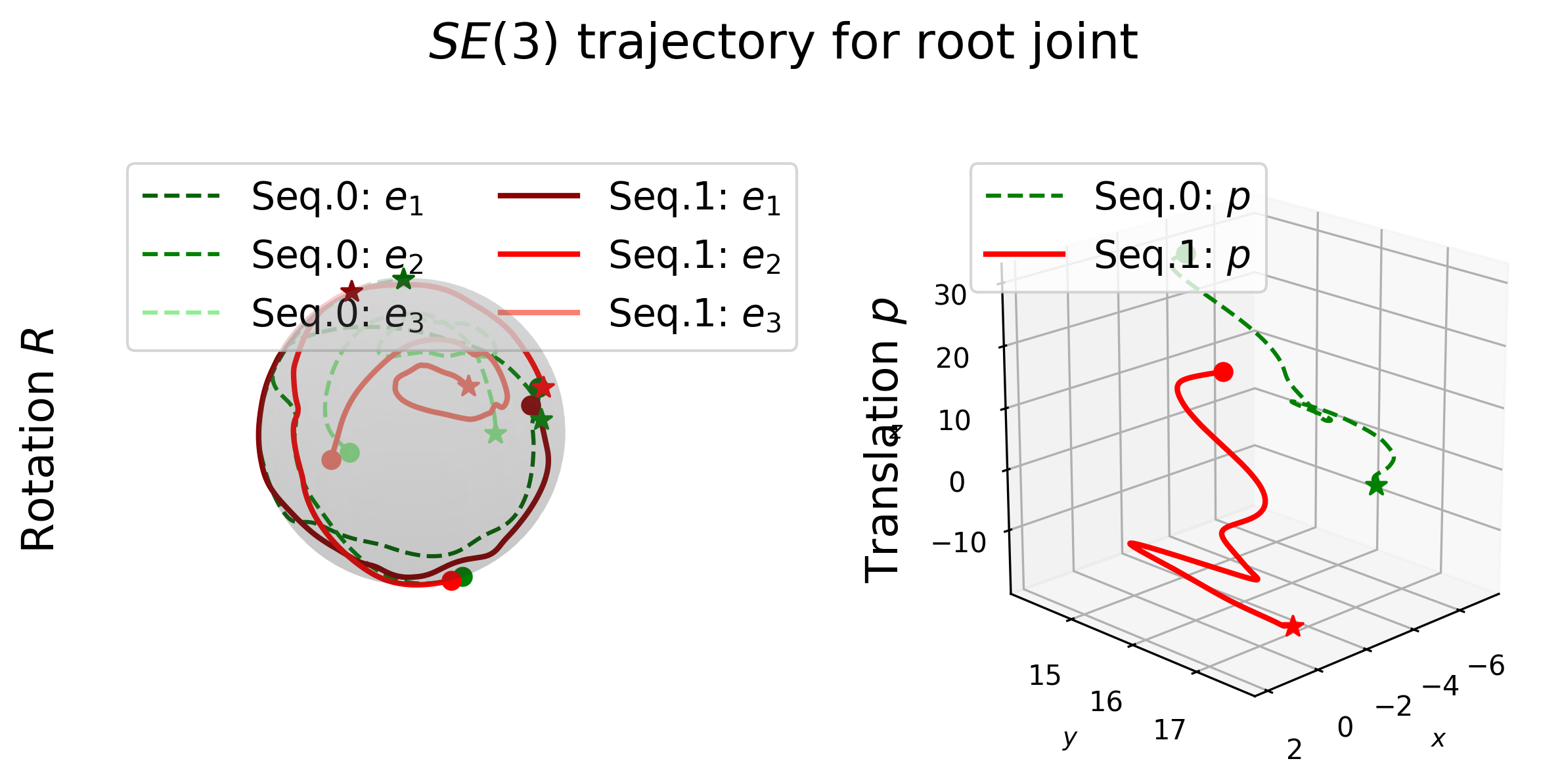

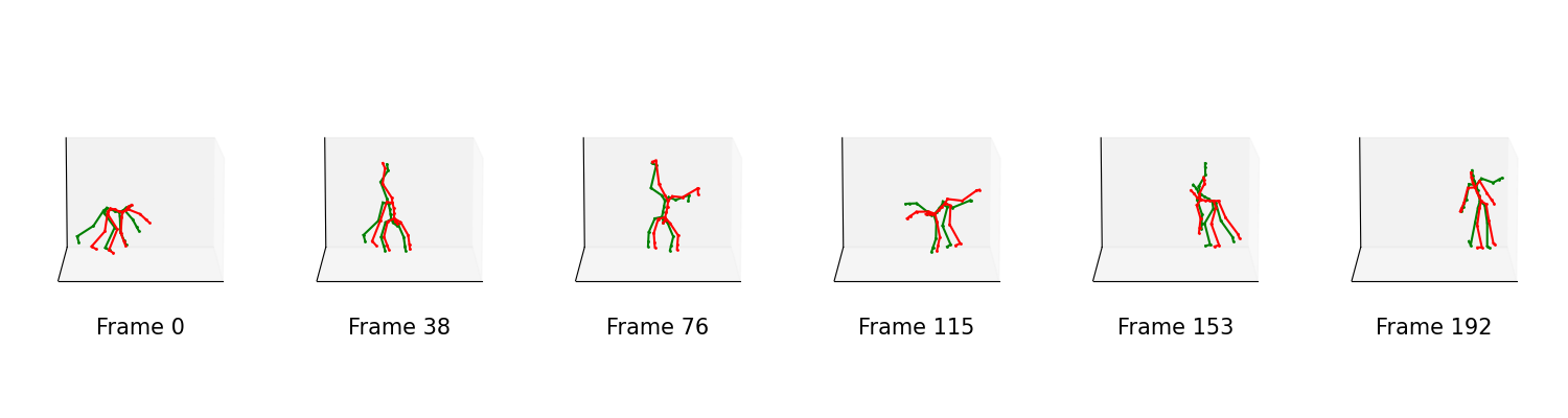
Figure 5: An overlay of Sequence 1 (green) and Sequence 2 (red) illustrates the natural variability in execution for the same subject. These visible differences in global paths and local joint rotations establish the baseline scale for evaluating reproduction errors.. a — Root joint in SE(3)., b — Selection of body joints in SO(3)., c — Skeleton renderings.
The learned pair \((L^\theta, F^\theta)\) defines a single autonomous discrete dynamical system. Consequently, two observed sequences can only be reproduced exactly if they are solutions to the same state-feedback law. Human motion, however, is internally driven by time-varying muscle actuation rather than a pure function of mechanical state. Since two repetitions of the same movement involve different actuation histories, a shared \(F^\theta\) must necessarily compromise where the sequences diverge (Figure 5). The learned force should therefore be viewed as an effective state-feedback approximation of the actuated dynamics. Accordingly, our objective is not exact reproduction, but rather to assess: (i) if the model faithfully captures the global skeletal movement, and (ii) if the per-sequence reproduction error remains below the inherent discrepancy between the two ground-truth recordings. This inter-sequence variability provides the natural benchmark for evaluating the model’s performance.
5.4.0.2 Setup and data curation.
We use human motion capture recordings of cartwheel movements from the Carnegie Mellon University Motion Capture Database (CMU MoCap) [39], a publicly available collection of human motion sequences recorded at \(120\) Hz using a marker-based optical capture system. The skeleton consists of \(B=23\) segments: a root joint in \(SE(3)\) (global pose) and \(22\) body joints in \(SO(3)\), namely the left and right hip, femur, tibia, foot, clavicle, humerus, radius and wrist, lower and upper back, lower and upper neck, thorax and head. We select Trials 6 and 7 from Subject 49 (Figure 5), converting the original Euler angles into rotation matrices. Prior to training, the raw motion capture data undergoes preprocessing to remove noise and edge effects. Each joint trajectory is smoothed along the time dimension using a Savitzky–Golay [40] filter with a window size of \(50\) frames and polynomial order \(6\).
A single model \((L^\theta, F^\theta)\) is trained jointly on both sequences, and each sequence is then reproduced by rolling the learned dynamics forward from its true initial configuration pair. Training on only two sequences intentionally tests the model’s ability to capture complex, high-dimensional coupled dynamics from extremely sparse data. We model the external force as a sum of two components, \(F^\theta = F^\theta_\mathrm{NL} + F^\theta_\mathrm{NN}\). The first, \(F^\theta_\mathrm{NL}\), is a nonlinear Rayleigh dissipation term in which the damping matrix \(D^\theta(R, p)\) varies with configuration. The second, \(F^\theta_\mathrm{NN}\), is an unconstrained neural network that imposes no structural constraints and can represent arbitrary nonlinear, non-dissipative, or energy-injecting effects from the human.
5.4.0.3 Results and Discussion.
*4|c| & Root rot.& Mean joint rot.& Root pos.
Sequence 1 (prediction error) & 0.193 & 0.186 & 0.887
Sequence 2 (prediction error) & 0.188 & 0.233 & 1.409
Ground truth discrepancy & 0.373 & 0.416 & 6.624


Figure 6: Per-timestep reproduction errors of cartwheel sequences. The gray baseline indicates the discrepancy between the two ground truth recordings. Reproduction errors remain consistently below the ground-truth variability. Error peaks align with phases of high recording divergence, where the shared state-feedback force must mediate between the two reference trajectories..
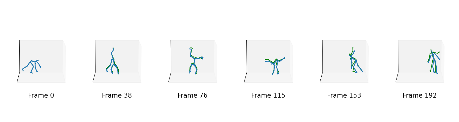
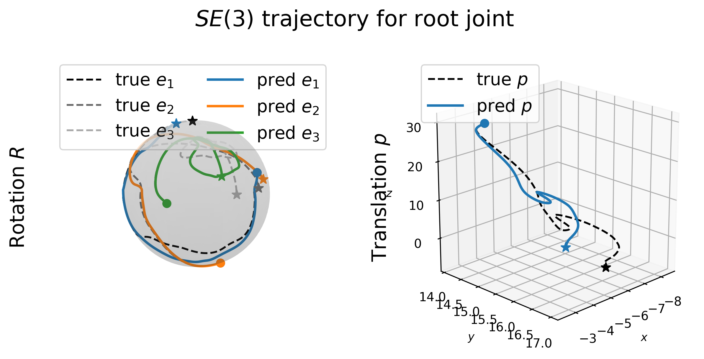

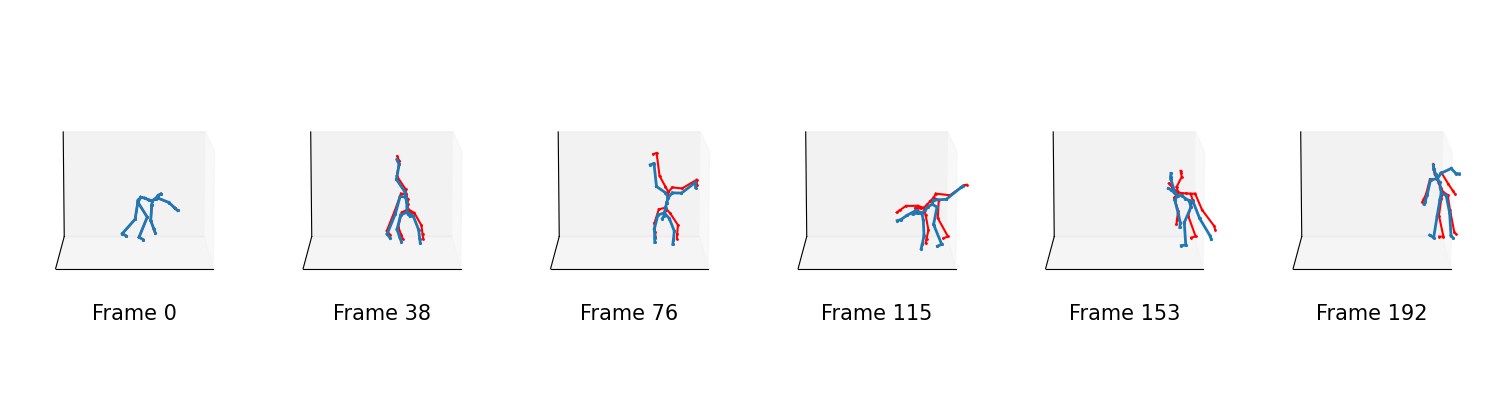


Figure 7: Qualitative comparison for cartwheel sequences. 7 (c)-7 (f) Top: skeletal renderings at uniform intervals (ground truth: green/red, prediction: blue), showing nearly coincident poses throughout the \(360^\circ\) rotation. 7 (c)-7 (f) Bottom: reconstructed root trajectories in \(SE(3)\) (left) and trajectories of selected joint rotation axes on the unit sphere, illustrating the high-fidelity reconstruction of \(SO(3)\) dynamics (right).. c — Sequence 1 (Trial 6)., f — Sequence 2 (Trial 7).
Table ¿tbl:tab:mocap95errors? and Figure 6 report the quantitative reproduction errors. Across all metrics, per-sequence errors remain consistently below the inter-sequence ground-truth discrepancy. This confirms that the model captures the specific characteristics of each motion individually rather than a "blurred" average. As expected, the error peaks align with phases where the two demonstrations diverge most, marking the regions where the shared state-feedback force must mediate between the two actuation histories.
Qualitative results in Figure 7 show that the predicted and ground-truth skeletons remain nearly coincident throughout the \(360^\circ\) rotation. The reconstructed joint trajectories on the unit sphere closely follow the recorded paths, with both sequences reproduced with comparable fidelity.
These results demonstrate that the LieDFLNN generalizes to real-world multibody systems without modifications to the model architecture. The discrete Lagrangian formulation naturally handles the product manifold \(SE(3) \times SO(3)^{B-1}\), treating each joint group element independently while capturing coupled skeletal dynamics through a shared interaction potential. By operating directly on Lie groups, the model avoids the singularities and wrapping artifacts of Euler angles identified in Experiment 1. The close qualitative agreement of the predictions despite the very limited training data suggests that the inductive bias introduced by the discrete Lagrangian formulation together with the product Lie group structure serves as an effective regularizer, compensating for the small amount of training data.
5.5 Experiment 5: Learning an unknown control on \(SO(3)\) with known Lagrangian↩︎
The preceding experiments learned the discrete Lagrangian and the external forces jointly. In this experiment, we consider the complementary identification problem: the Lagrangian of the system is assumed known, and only the control input is learned. This scenario is relevant in practice when the mechanical properties of a system (inertia, potential) are available from design specifications, but the system is driven by an unknown or unmodeled feedback controller whose behavior one wishes to identify from observed motion. This setting also validates the framework’s ability to isolate and recover individual dynamical components when others are fixed.
5.5.0.1 Setup and data generation.
We consider a single rigid body evolving on \(SO(3)\) in a gravitational field, using the Lagrangian from Example 1, governing equations as in Experiment 1, and known parameters \(J\), \(J_d\) and \(V\). The body is driven
by a PD attitude controller [41] (see also 11.5)
\[\label{eq:32exp532true32PD32control} \tau_{\mathrm{PD}}(R, \omega) = -K_R\, e_R(R, R_{\mathrm{f}}) - K_\omega\, \omega, \qquad e_R(R, R_{\mathrm{f}}) = \frac{1}{2}
\vex\!\left(R_{\mathrm{f}}^\top R - R^\top R_{\mathrm{f}}\right),\tag{18}\] which drives the attitude toward a fixed target \(R_{\mathrm{f}} \in SO(3)\). We set \(K_R = k_r I\)
and \(K_\omega = k_\omega I\), scaling the gains by a scalar representative inertia \(\bar{J} = \tfrac{1}{N}\sum_{i,j} J_{ij}\) (the mean of the entries of \(J\)), with \(k_r = 5.0\,\bar{J}\) and \(k_\omega = 1.0\,\bar{J}\). The training data consist of a single trajectory of \(N =
500\) timesteps with stepsize \(h = 0.05\), generated by integrating Eq. 12 –13 with \(\tau = \tau_{\mathrm{cons}} + \tau_{\mathrm{PD}}\) from an initial condition \((R_0, \omega_0)\) using the RK45 solver from scipy.integrate.solve_ivp. The rigid body has mass \(m = 0.5\) and center of mass offset \(\rho_\mathrm{com} = (0,\, 0.5,\, 1.0)^\top\), and diagonal inertia tensor \(J = \mathrm{diag}(1.521,\, 1.362,\, 1.211)\),
under gravitational acceleration \(g = 9.81\). We retain only the rotation sequence \(\{R_k\}_{k=0}^{N}\), neither angular velocities nor applied control inputs are observed.
We emphasize that learning from a single trajectory is a deliberately restricted setting. A state-feedback control can only be identified on the region of the state space visited by the observed motion. Accordingly, as in Experiment 4, the objective is faithful reproduction of the observed dynamics and recovery of the control along the trajectory, rather than generalization to unseen initial conditions.
5.5.0.2 Control parameterization and learning problem.
Following the structure of Eq. ?? , we parameterize the unknown control as \[\label{eq:32exp532learned32control} \tau^\theta(R, \omega) = C^\theta\, u^\theta(R, \omega),\tag{19}\] where \(C^\theta \in \mathbb{R}^{3 \times m}\) is a learnable input matrix and \(u^\theta : SO(3) \times \mathbb{R}^3 \to \mathbb{R}^m\) is a fully connected neural network taking the (flattened) rotation matrix and the angular velocity as inputs. The control is discretized in the same way as the external forces in Section 9.1, \[\tau^{\theta, \pm}_{d,k} = \frac{h}{2}\, \tau^\theta\!\left(R_k,\; \frac{\vex(W_k - W_k^\top)}{2h}\right),\] where the angular velocity argument is recovered from the observed increment \(W_k = R_k^\top R_{k+1}\), so that the model remains a function of positions only. Since the discrete Lagrangian is fixed, the loss 11 reduces to the residual of the discrete controlled Euler-Lagrange equations 10 alone, evaluated on the observed triplets \((R_{k-1}, R_k, R_{k+1})\). No regularization is required, as the regularity of the Lagrangian is guaranteed by construction.
The factorization \(\tau^\theta = C^\theta u^\theta\) is not unique; for any invertible \(S \in \mathbb{R}^{m \times m}\), the pair \((C^\theta S,\, S^{-1} u^\theta)\) yields the same torque. Unlike settings where the control input \(u\) is observed [42], here only the product \(\tau^\theta\) is identifiable. We therefore evaluate the accuracy of the total torque \(\tau^\theta\) rather than its individual factors. To remove the scale ambiguity during training, we normalize the columns of \(C^\theta\) to have unit norm.
5.5.0.3 Results and discussion.
After training, the learned system is rolled out from the true initial pair \((R_0, R_1)\) by solving the discrete controlled Euler-Lagrange equations 10 forward in time with the known Lagrangian and the learned control \(\tau^\theta\), as described in the inference procedure. Figure 8 summarizes the results.
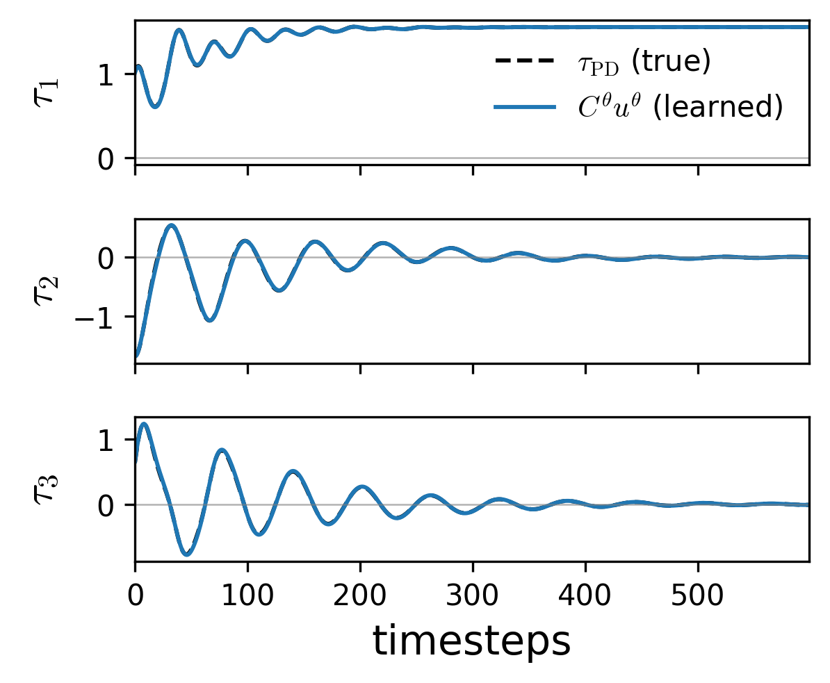


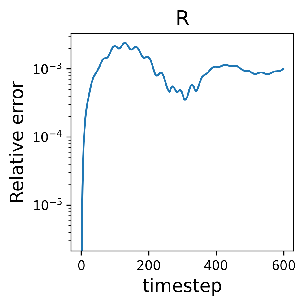
Figure 8: Identifying a PD controller on \(SO(3)\) with a known Lagrangian. Results are obtained from a single 600-step trajectory. (8 (a), 8 (c)): the learned torque \(\tau^\theta\) (solid) accurately recovers the true PD control signal (dashed) along the observed trajectory. (8 (b), 8 (d)): rollout of the identified system showing faithful reproduction of the stabilizing motion toward the target \(R_\mathrm{f}\), with errors remaining stable over the long-term horizon..
The learned control \(\tau^\theta\) matches the true PD control signal closely (Figure 8 (a)), capturing both the large transient torques at the start of the motion and the decay as the error \(e_R\) vanishes. The relative control error (Figure 8 (c)) remains low throughout the sequence, peaking slightly during the rapid initial transient.
The resulting rollout (Figure 8 (b)) follows the ground-truth stabilizing trajectory on the sphere, maintaining a low relative rotation error over the full 600-step horizon (Figure 8 (d)).
Two aspects of this experiment are worth emphasizing. First, the discrete variational structure successfully disentangles the unknown control from the known conservative dynamics using only position data. The ability to recover the control signal without observing torques or velocities confirms the strength of the LieDFLNN as a tool for system identification in closed-loop settings. Second, in line with Remark [remark:32exp532identifiability], we evaluate the identifiable product \(C^\theta u^\theta\) rather than its factors. The factorization 19 nevertheless provides the interface through which a known actuation structure could be imposed by fixing \(C\), which we regard as a natural extension toward underactuated systems.
6 CONCLUSIONS↩︎
In this work we have introduced a framework for learning mechanical systems using discrete forced Euler-Lagrange equations on Lie groups. By embedding the geometric structure of \(SO(3)\) and \(SE(3)\) directly into the variational integrator, we eliminate the coordinate singularities and geometric drift common in Euclidean baselines. Our experiments demonstrate that the LieDFLNN maintains high-fidelity predictions across large-angle rotations and long-term rollouts. The model recovers complex dynamics from position data alone and scales to high-dimensional multibody systems like human motion. Furthermore, the framework is modular, capable of identifying full dynamics or isolating specific components—such as unknown control laws—when the Lagrangian is known.
7 ACKNOWLEDGMENTS↩︎
The authors would like to express gratitude to Benjamin Kwanen Tapley and Jacob Goodman for their valuable discussions during the preparation of this paper. This research was supported by EU through MSCA-SE: REMODEL (Project ID: 101131557), and by the Research Council of Norway through PhysML (No. 338779). DMdD acknowledges financial support from the Spanish Ministry of Science and Innovation under grants PID2022-137909NB-C21, PCI2024-155047-2 and from the Severo Ochoa Programme for Centres of Excellence in R&D (CEX2023-001347-S). The data used in this project was obtained from mocap.cs.cmu.edu. The database was created with funding from NSF EIA-0196217.
8 BASIC NOTIONS ABOUT \(SO(3)\) AND \(SE(3)\)↩︎
8.1 The Lie group \(SO(3)\)↩︎
Consider the 3D rotation group \(SO(3) = \{ R\in\mathbb{R}^{3\times 3} : R^\top R = R R^\top = I, \, \det(R) =1\}\). Its Lie algebra \(\mathfrak{so}(3)=\{\Omega \in \mathbb{R}^{3\times 3} : \Omega^\top = -\Omega \}\) can be identified with \(\mathbb{R}^3\) via the hat map \[\hat{}:\mathbb{R}^3 \to \mathfrak{so}(3),\qquad \widehat{(a,b,c)}=\begin{pmatrix} 0&-c&b\\ c&0&-a\\ -b&a&0 \end{pmatrix},\] and we let \(\vex: \mathfrak{so}(3) \to \mathbb{R}^3\) be its inverse.
8.1.0.1 Left and Right multiplications in \(SO(3)\).
Let \(R\in SO(3)\). The Left and Right multiplications by \(R\) on \(SO(3)\), \(\mathcal{L}_R, \mathcal{R}_R : SO(3) \to SO(3)\) are \[\mathcal{L}_{R}(Q) = RQ, \qquad \mathcal{R}_{R}(Q) = QR.\] The tangent lifts at the identity of the Left and Right multiplications \(T\mathcal{L}_R, T\mathcal{R}_R :\mathfrak{so}(3) \to T_R SO(3)\) are given by \[T \mathcal{L}_R (\hat{\omega}) = \frac{d}{dt}\Bigg|_{t=0} \mathcal{L}_{R} Q(t) = R\hat{\omega}, \qquad T \mathcal{R}_R (\hat{\omega}) = \frac{d}{dt}\Bigg|_{t=0} \mathcal{R}_{R} Q(t) = \hat{\omega} R\] where \(Q(t)\) is a curve on \(SO(3)\) such that \(Q(0) = I_3\) and \(\Dot{Q}(0)= \hat{\omega} \in \mathfrak{so}(3)\). The cotangent lifts of the Left and Right multiplications \(\mathcal{L}_R^*, \mathcal{R}_R^*: (T_R SO(3))^* \to \mathfrak{so}(3)^*\) are the maps such that \[\langle \mathcal{L}_R^* (\Pi), \hat{\omega} \rangle = \langle \Pi, T \mathcal{L}_R (\hat{\omega}) \rangle, \qquad \langle \mathcal{R}_R^* (\Pi), \hat{\omega} \rangle = \langle \Pi, T \mathcal{R}_R (\hat{\omega}) \rangle\] for any \(\hat{\omega}\in \mathfrak{so}(3)\). Define the pairing \(\langle \Pi, \hat{\omega} \rangle = \trace(\Pi^\top \hat{\omega})\), then one has \[\mathcal{L}_{R}^* (\Pi) = R^\top \Pi, \qquad \mathcal{R}_{R}^* (\Pi) = \Pi R^\top.\]
8.1.0.2 Exp and Log maps in \(SO(3)\).
The exponential map \(\exp : \mathfrak{so}(3) \to SO(3)\) is given by \[R = \exp(\widehat{\omega}) := I + \frac{\sin\theta}{\theta} \widehat{\omega} + \frac{1-\cos\theta}{\theta^2} \widehat{\omega}^2, \qquad \theta := \| \omega \|.\] Taking the trace on both sides \[\begin{align} \trace(R) = 3 + \frac{1-\cos\theta}{\theta^2} 2 \theta^2 \quad \Rightarrow \quad \theta = \cos^{-1} \left( \frac{\trace(R)-1}{2} \right). \end{align}\] Also \[\begin{align} R - R^\top = \frac{2 \sin\theta}{\theta} \widehat{\omega} \quad \Rightarrow \quad \widehat{\omega} = \frac{\theta}{2\sin\theta} (R-R^\top), \end{align}\] so \(\log: SO(3) \to \mathfrak{so}(3)\) is given by \[\widehat{\omega} = \log(R) := \frac{\theta}{2\sin\theta} (R-R^\top), \qquad \theta := \cos^{-1} \left( \frac{\trace(R)-1}{2} \right).\]
8.2 The Lie group \(SE(3)\)↩︎
Consider the group of 3D rotations and translations \(SE(3) \simeq SO(3) \times \mathbb{R}^3\) and its Lie algebra \(\mathfrak{se}(3) \simeq \mathbb{R}^3 \times \mathbb{R}^3\). Let \(g\in SE(3)\), \(\xi\in \mathfrak{se}(3)\), then \[g=\begin{bmatrix} R & p \\ 0 & 1 \end{bmatrix}, \quad g^{-1}=\begin{bmatrix} R^\top & -R^\top p \\ 0 & 1 \end{bmatrix}, \quad\xi=\begin{bmatrix} \hat{\omega} & v \\ 0 & 0 \end{bmatrix}, \qquad R\in SO(3), \hat{\omega} \in \mathfrak{so}(3), p, v\in\mathbb{R}^3.\]
8.2.0.1 Left and Right multiplications in \(SO(3)\).
The Left and Right multiplications by \(g=(R, p)\) on \(SE(3)\), \(\mathcal{L}_g, \mathcal{R}_g : SE(3) \to SE(3)\) are \[\mathcal{L}_{(R,p)}(Q,y) = (RQ, p+Ry), \qquad \mathcal{R}_{(R,p)}(Q,y) = (QR, y+Qp).\] The tangent lifts of the Left and Right multiplications \(T \mathcal{L}_g, T \mathcal{R}_g:\mathfrak{se}(3) \to T_g SE(3)\) are given by \[T \mathcal{L}_g (\hat{\omega}, v) = \frac{d}{dt}\Bigg|_{t=0} \mathcal{L}_{(R, p)} (Q(t), y(t)) = \frac{d}{dt}\Bigg|_{t=0} (RQ(t), p+ Ry(t)) = (R\hat{\omega}, Rv)\] and \[T \mathcal{R}_g (\hat{\omega}, v) = \frac{d}{dt}\Bigg|_{t=0} \mathcal{R}_{(R, p)} (Q(t), y(t)) = \frac{d}{dt}\Bigg|_{t=0} (Q(t)R, Q(t)p+ y(t)) = (\hat{\omega} R, \hat{\omega} p + v)\] where \((Q(t), y(t))\) is a curve on \(SE(3)\) such that \((Q(0), y(0)) = (I_3,0)\) and \((\Dot{Q}(0), \Dot{y}(0)) = (\hat{\omega},v) \in \mathfrak{se}(3)\). The cotangent lifts of the Left and Right multiplications \(\mathcal{L}_g^*, \mathcal{R}_g^*: (T_g SE(3))^* \to \mathfrak{se}(3)^*\) are the maps such that \[\langle \mathcal{L}_g^* (\tau), \xi \rangle = \langle \tau, T \mathcal{L}_g (\xi) \rangle, \qquad \langle \mathcal{R}_g^* (\tau), \xi \rangle = \langle \tau, T \mathcal{R}_g (\xi) \rangle.\] for any \(\xi\in \mathfrak{se}(3)\). For \(\tau = (\Pi, F) \in \mathfrak{so}(3)^* \times \mathbb{R}^3\) and \(\xi = (\hat{\omega}, v) \in \mathfrak{so}(3) \times \mathbb{R}^3\), let us define the pairing \[\langle (\Pi, F), (\hat{\omega}, v) \rangle = \trace(\Pi^\top \hat{\omega}) + F^\top v.\] One can then compute that \[\mathcal{L}_{(R,p)}^* (\Pi, F) = (R^\top \Pi, R^\top F), \qquad \mathcal{R}_{(R,p)}^* (\Pi, F) = \left(\Pi R^\top - \frac{1}{2} \widehat{F \times p} , F \right).\] Above we have used \[F^\top (\hat{\omega} p ) = F \cdot (\omega \times p) = \omega \cdot (p \times F) = - \frac{1}{2} \trace ( \widehat{F \times p}^\top \hat{\omega} ).\]
8.2.0.2 Exp and Log maps in \(SE(3)\).
The exponential map is given by \[\exp : \mathfrak{se}(3) \to SE(3), \qquad (\omega, v) \mapsto (R, Av)\] where, for \(\theta := \| \omega \|\), \[R = I + \frac{\sin\theta}{\theta} \widehat{\omega} + \frac{1-\cos\theta}{\theta^2} \widehat{\omega}^2, \qquad A = I + \frac{1-\cos{\theta}}{\theta^2} \hat{\omega} + \frac{\theta - \sin{\theta}}{\theta^3} \hat{\omega}^2.\] Its inverse, namely the logarithmic map, is given by \[\log : SE(3) \to \mathfrak{se}(3), \qquad (R, p) \mapsto (\omega, A^{-1}p)\] where, for \(\theta := \cos^{-1} \left( \frac{\trace(R)-1}{2} \right)\), \[\widehat{\omega} = \log(R) := \frac{\theta}{2\sin\theta} (R-R^\top), \qquad A^{-1} = I - \frac{1}{2} \hat{\omega} + \left( \frac{1}{\theta^2} - \frac{1+\cos{\theta}}{2\theta \sin{\theta}} \right) \hat{\omega}^2\]
In numerics, when \(\theta \to 0\) one encounters division by zero. It is then desirable to replace the above close forms with e.g. Taylor approximations. More precisely, for small \(\theta\) one has \[\begin{align} \frac{\sin{\theta}}{\theta} &\approx 1 - \frac{\theta^2}{6}, \quad \frac{1-\cos{\theta}}{\theta^2} \approx \frac{1}{2} - \frac{\theta^2}{24} ,\quad \frac{\theta - \sin{\theta}}{\theta^3} \approx \frac{1}{6} - \frac{\theta^2}{120}, \quad \frac{1}{\theta^2} - \frac{1+\cos{\theta}}{2\theta\sin{\theta}} \approx \frac{1}{12} + \frac{\theta^2}{720}, \end{align}\] hence \[\exp(\omega, v) \approx \left( I + \hat{\omega} + \frac{1}{2} \hat{\omega}^2, \left( I + \frac{1}{2} \hat{\omega} + \frac{1}{6} \hat{\omega}^2 \right) v \right)\] and \[\log(R,p) \approx ({\omega}, v) = \left( \frac{3}{6-\theta^2} (R-R^\top), \left( I - \frac{1}{2} \hat{\omega} + \frac{1}{12} \hat{\omega}^2 \right) p \right).\] In particular, using the first order approximation for the exp map, we obtain \[(W, z ) = \exp(h \omega, h v) \approx \left( I + h \hat{\omega}, \left(I + \frac{1}{2} h \hat{\omega} \right) h v \right)\] from which one can compute \[\hat{\omega} \approx \frac{W - I}{h}, \qquad v \approx \left(I + \frac{1}{2} h \hat{\omega} \right)^{-1} \frac{z}{h} \approx \left(I - \frac{1}{2} h \hat{\omega} \right) \frac{z}{h}\] where we have used the Neumann series to approximate the inverse of a matrix. To make sure that \(\hat{\omega}\) is skew symmetric one should take the skew symmetric part of \(\frac{W-I}{h}\), leading to \[\hat{\omega} \approx \mathrm{skew} \left(\frac{W - I}{h}\right) = \frac{1}{2h} (W - W^\top).\] The same is obtained using the first order approximation of the log map: \[(\hat{\omega}_k, z_k ) = \frac{1}{h} \log(W_k, z_k) \approx \left( \frac{1}{2h} (W_k - W_k^\top), \left(I - \frac{1}{2} h \hat{\omega}_k \right) \frac{z_k}{h} \right).\]
9 DETAILED DERIVATION OF THE DISCRETE EULER-LAGRANGE EQUATIONS (DEL)↩︎
9.1 Discrete forced rigid body equations on \(SO(3)\)↩︎
Let \(\eta\in\mathbb{R}^3\). The discrete Euler-Lagrange equation 5 rewrites \[\begin{align} \langle{\mathcal{L}}^*_{R_k} \frac{\partial \bar{L}_{d,k}}{\partial R_k}, \hat{\eta} \rangle &- \langle{\mathcal{R}}^*_{W_k} \frac{\partial \bar{L}_{d,k}}{\partial W_k}, \hat{\eta} \rangle + \langle{\mathcal{L}}^*_{W_{k-1}} \frac{\partial \bar{L}_{d,k-1}}{\partial W_{k-1}}, \hat{\eta} \rangle + \langle {\tau_{\mathrm{ext}}}^-_{d,k} , \eta \rangle + \langle {\tau_{\mathrm{ext}}}^+_{d,k-1}, \eta \rangle \\ &= \trace\left( \left( R_k^\top \frac{\partial \bar{L}_{d,k}}{\partial R_k} - \frac{\partial \bar{L}_{d,k}}{\partial W_k} W_k + W_{k-1} \frac{\partial \bar{L}_{d,k}}{\partial W_{k-1}} + \frac{1}{2} (\widehat{{\tau_{\mathrm{ext}}}^-_{d,k}}+ \widehat{{\tau_{\mathrm{ext}}}^+_{d,k-1}}) \right)^\top \hat{\eta} \right) \\ &= \trace ( A^\top \hat{\eta}) = 0. \end{align}\] The above holds for any \(\eta\) if and only if \(A = A^\top\), that is 6 .
9.2 Discrete forced rigid body equations on \(SE(3)\)↩︎
Let \(\xi=(\hat{\eta},\mu)\in\mathfrak{se}(3)\). The discrete Euler-Lagrange equation 5 rewrites \[\begin{align} \langle{\mathcal{L}}^*_{(R_k,p_k)} & \left( \frac{\partial \bar{L}_{d,k}}{\partial R_k}, \frac{\partial \bar{L}_{d,k}}{\partial p_k} \right), \xi\rangle - \langle{\mathcal{R}}^*_{(W_k,z_k)} \left( \frac{\partial \bar{L}_{d,k}}{\partial W_k}, \frac{\partial \bar{L}_{d,k}}{\partial z_k} \right), \xi\rangle + \langle{\mathcal{L}}^*_{(W_{k-1},z_{k-1})} \left( \frac{\partial \bar{L}_{d,k-1}}{\partial W_{k-1}}, \frac{\partial \bar{L}_{d,k-1}}{\partial z_{k-1}} \right), \xi\rangle& \\ =& \, \trace\left( \left( R_k^\top \frac{\partial \bar{L}_{d,k}}{\partial R_k} - \frac{\partial \bar{L}_{d,k}}{\partial W_k} W_k^\top + \frac{1}{2} \left( \frac{\partial \bar{L}_{d,k}}{\partial z_k} \times z_k \right)^\wedge + W_{k-1}^\top \frac{\partial \bar{L}_{d,k-1}}{\partial W_{k-1}} + \frac{1}{2} (\widehat{{\tau_\mathrm{ext}}^-_{d,k}}+ \widehat{{\tau_\mathrm{ext}}^+_{d, k-1}}) \right)^\top \hat{\eta} \right) \\ & + \left( R_k^\top \frac{\partial \bar{L}_{d,k}}{\partial p_k} - \frac{\partial \bar{L}_{d,k}}{\partial z_{k}} + W_{k-1}^\top \frac{\partial \bar{L}_{d,k-1}}{\partial z_{k-1}} + ({f_\mathrm{ext}}^-_{d,k}+{f_\mathrm{ext}}^+_{d,k-1}) \right)^\top \mu \\ =& \, \trace(A^\top \hat{\eta}) + b^\top \mu = 0. \end{align}\] The above equation holds true for any \((\hat{\eta}, \mu)\) if and only if \(A=A^\top\) and \(b=0\), that is, \[\begin{align} R_k^\top \frac{\partial \bar{L}_{d,k}}{\partial R_k} - \frac{\partial \bar{L}_{d,k}}{\partial R_k}^\top R_k + W_k \frac{\partial \bar{L}_{d,k}}{\partial W_k}^\top - \frac{\partial \bar{L}_{d,k}}{\partial W_k} W_k^\top + \left( \frac{\partial \bar{L}_{d,k}}{\partial z_k} \times z_k \right)^\wedge & \nonumber \\ + W_{k-1}^\top \frac{\partial \bar{L}_{d,k-1}}{\partial W_{k-1}} - \frac{\partial \bar{L}_{d,k-1}}{\partial W_{k-1}}^\top W_{k-1} + (\widehat{{\tau_\mathrm{ext}}^-_{d,k}}+ \widehat{{\tau_\mathrm{ext}}^+_{d, k-1}}) &= 0, \\ R_k^\top \frac{\partial \bar{L}_{d,k}}{\partial p_k} - \frac{\partial \bar{L}_{d,k}}{\partial z_{k}} + W_{k-1}^\top \frac{\partial \bar{L}_{d,k-1}}{\partial z_{k-1}} + ({f_\mathrm{ext}}^-_{d,k}+{f_\mathrm{ext}}^+_{d,k-1}) &= 0, \end{align}\] which correspond to equations 8 9 .
Example 3 (Rigid body). Let us consider the Lagrangian of a rigid body \[\bar{L} (R, p, \omega, v) = T(\omega, v) - V(R, p) = \frac{1}{2} \omega^\top J \omega + \frac{1}{2} m (v + \hat{\omega} \rho_{COM})^\top (v + \hat{\omega} \rho_{COM}) - V(R, p).\] where \(J\) is the inertia matrix for vector representation, \(m>0\) the mass, \(\rho_{COM}\in\mathbb{R}^3\) the center of mass vector in the body frame, \(v +\hat{\omega}\rho_{\text{COM}} = \frac{\partial p}{\partial t} + \frac{\partial R}{\partial t}\rho_{\text{COM}}\) the velocity of the center of the mass in the global frame (\(p + R\rho_\text{COM}\) is its position). The discrete Lagrangian is \[\begin{align} \bar{L}_{d,k} =& \, \bar{L}_d(R_k,p_k,W_k,z_k) = h \bar{L} \left(R_k, p_k, \frac{W_k - I}{h}, \frac{z_k }{h} \right) \nonumber \\ =&\, \frac{1}{h} (\trace(J_d) - \trace(W_k J_d)) + \frac{1}{2h} m (z_k + (W_k - I)\rho_{\text{COM}})^\top (z_k + (W_k - I)\rho_{\text{COM}}) - h V(R_k, p_k) \nonumber \\ \end{align}\] where \(J_d\) satisfies \(J = \trace({J_d}) I - J_d\) as noted in [35]. The partial derivatives of \(\bar{L}_d\) with respect to \(R\), \(p\), \(W\) and \(z\) are \[\begin{align} \frac{\partial \bar{L}_{d}}{\partial R} &= - h \frac{\partial V}{\partial R} , & \frac{\partial \bar{L}_{d}}{\partial W} &= - \frac{1}{h} J_d + \frac{1}{h} m z_k \rho_{COM}^\top -\frac{1}{h} m \rho_{COM} \rho_{COM}^\top,\\ \frac{\partial \bar{L}_{d}}{\partial p} &= - h \frac{\partial V}{\partial p} , & \frac{\partial \bar{L}_{d}}{\partial z} & = \frac{1}{h} m z + \frac{1}{h} m (W_k -I)\rho_{COM} \end{align}\] and we can replace them in 8 9 to find \[\begin{align} \label{eq:32DEL32SE332version32with32A32example} -h \left(R_k^\top \frac{\partial V_{k}}{\partial R} - \left(\frac{\partial V_{k}}{\partial R}\right)^\top R_k \right) + \frac{1}{h} \left( J_d W_k^\top - W_k J_d \right) + \frac{1}{h} \left( J_d W_{k-1} - W_{k-1}^\top J_d \right) & \nonumber \\ + \frac{1}{h} m \left( W_k \rho_{\mathrm{COM}} z_k^\top - z_k \rho_{\mathrm{COM}}^\top W_k^\top + W_{k-1}^\top z_{k-1} \rho_{\mathrm{COM}}^\top - \rho_{\mathrm{COM}} z_{k-1}^\top W_{k-1} \right) & \nonumber \\ + \frac{1}{h} m \left( \rho_{\mathrm{COM}} \rho_{\mathrm{COM}}^\top (W_k^\top + W_{k-1}) - (W_k + W_{k-1}^\top) \rho_{\mathrm{COM}} \rho_{\mathrm{COM}}^\top \right) & \nonumber \\ + \frac{1}{h} m \left( (W_k - I) \rho_{\mathrm{COM}} \times z_k \right)^\wedge + (\widehat{{\tau_\mathrm{ext}}^-_{d,k}}+ \widehat{{\tau_\mathrm{ext}}^+_{d, k-1}}) &=0 \\ \label{eq:32DEL32SE332version32with32b32example} - h R_k^\top \frac{\partial V_{k}}{\partial p} + \frac{1}{h} m \left( W_{k-1}^\top z_{k-1} - z_k + 2 I \rho_{\mathrm{COM}} - (W_{k-1}^\top + W_k) \rho_{\mathrm{COM}} \right) + ({f_\mathrm{ext}}^-_{d,k}+{f_\mathrm{ext}}^+_{d,k-1}) &= 0. \end{align}\] {#eq: sublabel=eq:eq:32DEL32SE332version32with32A32example,eq:eq:32DEL32SE332version32with32b32example} with \(R_{k+1} = R_k W_k\), \(p_{k+1} = p_k + R_k z_k\).
9.3 Discrete forced equations on \(SE(3) \times SO(3)\)↩︎
We consider two bodies and choose \(SE(3) \times SO(3)\) as configuration space. The state and velocity of body 1 at timestep \(k\) is given by \((R_{1,k}, p_{1,k}, \omega_{1,k}, v_{1,k}) \in SE(3) \times \mathfrak{se}(3)\), while for body 2 we have \((R_{2,k}, \omega_{2,k}) \in SO(3) \times \mathfrak{so}(3)\). The discrete Lagrangian \(\bar{L}_d:SE(3) \times SE(3) \times SO(3) \times SO(3) \to \mathbb{R}\) is \[\begin{align} \bar{L}_{d,k} &= \bar{L}_{d,1,k} + \bar{L}_{d,2,k} - h V_{\mathrm{int},k} \\ &= \bar{L}_{d,1} (R_{1,k}, p_{1,k}, W_{1,k}, z_{1,k}) + \bar{L}_{d,2} (R_{2,k}, W_{2,k}) - h V_\mathrm{int} (R_{1,k}, p_{1,k}, R_{2,k}) \end{align}\] where \(\bar{L}_{d,1}: SE(3)\times SE(3) \to \mathbb{R}\) is the discrete Lagrangian for body \(1\), \(\bar{L}_{d,2}: SO(3)\times SO(3) \to \mathbb{R}\) is the discrete Lagrangian for body \(2\), and we have assumed that the interaction potential \(V_{\mathrm{int}} : SE(3) \times SO(3) \to \mathbb{R}\) depends on positions only. For readability, we also assume that there are no external forces. The system of equations corresponding to the Euler-Lagrange equation 5 is then \[\begin{align} \tag{20} R_{1,k}^\top \left( \frac{\partial \bar{L}_{d,1,k}}{\partial R_{1,k}} + \frac{\partial V_{\mathrm{int},k}}{\partial R_{1,k}} \right) - \left( \frac{\partial \bar{L}_{d,1,k}}{\partial R_{1,k}} + \frac{\partial V_{\mathrm{int},k}}{\partial R_{1,k}} \right)^\top R_{1,k} + \left( \frac{\partial \bar{L}_{d,1,k}}{\partial z_{1,k}} \times z_{1,k} \right)^\wedge & \nonumber \\ + W_{1,k} \frac{\partial \bar{L}_{d,1,k}}{\partial W_{1,k}}^\top - \frac{\partial \bar{L}_{d,1,k}}{\partial W_{1,k}} W_{1,k}^\top + W_{1,k-1}^\top \frac{\partial \bar{L}_{d,1,k-1}}{\partial W_{1,k-1}} - \frac{\partial \bar{L}_{d,1,k-1}}{\partial W_{1,k-1}}^\top W_{1,k-1} &= 0, \\ \tag{21} R_{2,k}^\top \left( \frac{\partial \bar{L}_{d,2,k}}{\partial p_{2,k}} + \frac{\partial V_{\mathrm{int},k}}{\partial p_{2,k}} \right)- \frac{\partial \bar{L}_{d,2,k}}{\partial z_{2,k}} + W_{2,k-1}^\top \frac{\partial \bar{L}_{d,2,k-1}}{\partial z_{2,k-1}} &= 0, \\ \tag{22} R_{2,k}^\top \left( \frac{\partial \bar{L}_{d,2,k}}{\partial R_{2,k}} - \frac{\partial \bar{L}_{d,2,k}}{\partial R_{2,k}}^\top \right) - \left( \frac{\partial \bar{L}_{d,2,k}}{\partial W_{2,k}} - \frac{\partial \bar{L}_{d,2,k}}{\partial W_{2,k}}^\top \right) W_{2,k} + W_{2,k-1} \left( \frac{\partial \bar{L}_{d,2,k}}{\partial W_{2,k-1}} - \frac{\partial \bar{L}_{d,2,k}}{\partial W_{2,k-1}}^\top \right) &= 0, \end{align}\] with \(R_{1,k+1} = R_{1,k} W_{1,k}\), \(p_{1,k+1} = p_{1,k} + R_{1,k} z_{1,k}\) and \(R_{2,k+1} = R_{2,k} W_{2,k}\).
10 REGULAR LAGRANGIAN↩︎
10.0.0.1 Discrete regular Lagrangian.
Let us consider the discrete Lagrangian of a rigid body evolving on \(SE(3)\) (see Example 3) \[\begin{align} \bar{L}_d (R_k, p_k, W_k, z_k) &= hL \left(R_k, p_k, \frac{W_k -I}{h}, \frac{z_k}{h} \right) \\ &= \frac{1}{h} \trace((I-W_k)J_d) + \frac{m}{2h} \| X_k \|^2 - hV_d(p_k,R_k), \end{align}\] where \(X_k = z_k + (W_k-I)\rho_{\mathrm{COM}}\), \(J_d\) is such that \(J = \trace(J_d)I - J_d\), \(J\) is the inertia matrix, \(m\) is the mass and \(\rho_\mathrm{COM}\) the position of the center of mass (\(\mathrm{COM}\)). \(\bar{L}_d\) is regular if the Hessian with respect to the increments \[\mathbb{H} = \begin{bmatrix} \frac{\partial^2 \bar{L}_d}{\partial z^2} & \frac{\partial^2 \bar{L}_d}{\partial z \partial W} \\[2pt] \frac{\partial^2 \bar{L}_d}{ \partial W \partial z} & \frac{\partial^2 \bar{L}_d}{\partial W^2} \end{bmatrix} =: \begin{bmatrix} \mathbb{H}_{zz} & \mathbb{H}_{zW} \\ \mathbb{H}_{Wz} & \mathbb{H}_{WW} \end{bmatrix}\] is non-singular [35]. Below we provide the explicit computation of \(\mathbb{H}\).
10.0.0.2 First variations (discrete momenta).
The discrete momenta are the first variation of \(\bar{L}_d\) with respect to a variation \((\delta z, \delta W)\). The variation of \(\bar{L}_d\) with
respect to \(\delta z\) is the usual gradient with respect to \(z_k \in \mathbb{R}^3\) \[\delta_z \bar{L}_d = \frac{\partial \bar{L}_d}{\partial z_k} = \frac{m}{h}
X_k .\] For variations with respect to \(\delta W\) we cannot compute the standard partial derivative as \(W \in SO(3)\). We use the Lie algebra \(\mathfrak{so}(3)\) and perturb \(W_k\) in the direction \(\eta\in\mathbb{R}^3\): \[W_k (\epsilon) = W_k
\exp(\epsilon\hat{\eta}).\] The first variation (discrete momentum) is given by \[\begin{align} \delta_W \bar{L}_d &= \left. \frac{d}{d\epsilon} \right|_{\epsilon=0} \bar{L}_d (R_k, p_k, W_k \exp(\epsilon \hat{\eta}),
z_k) \\ & = \left. \frac{d}{d\epsilon} \right|_{\epsilon=0} \frac{1}{h} \trace((I - W_k \exp(\epsilon\hat{\eta})) J_d) + \left. \frac{d}{d\epsilon} \right|_{\epsilon=0} \frac{m}{2h} \| z_k + (W_k\exp(\epsilon \hat{\eta})-I) \rho_{\mathrm{COM}} \|^2
\end{align}\] For the first term we have \[\begin{align} \left. \frac{d}{d\epsilon} \right|_{\epsilon=0} \frac{1}{h} \trace((I - W_k \exp(\epsilon\hat{\eta})) J_d) & = -\frac{1}{h} \trace (W_k \hat{\eta} J_d) =
-\frac{1}{h} \trace (J_d W_k \hat{\eta} ) \\ & = \frac{1}{h} \vex ( J_d W_k - W_k^\top J_d) \cdot \eta =: M_{k,\mathrm{rot}} \cdot \eta
\end{align}\] where we have used the property \(\left. \frac{d}{d\epsilon} \right|_{\epsilon=0} \exp(\epsilon \hat{\eta}) = \hat{\eta}\) and the trace identity \(\trace(A \hat{b}) =
\vex(A^\top -A) \cdot b\) with \(\vex\) the inverse of the hat operator.
For the second term \[\begin{align} \left. \frac{d}{d\epsilon} \right|_{\epsilon=0} \frac{m}{2h} \| z_k + (W_k\exp(\epsilon \hat{\eta})-I) \rho_{\mathrm{COM}} \|^2 = \frac{m}{h} X_k \cdot (W_k \hat{\eta} \rho_\mathrm{COM}) = -
\frac{m}{h} X_k \cdot (W_k \hat{\rho}_\mathrm{COM} \eta)
\end{align}\] where we have used \(\hat{v}w = v \times w = - w \times v = - \hat{w}v\). Now \[X_k \cdot (W_k \hat{\rho}_\mathrm{COM} \eta) = (W_k \hat{\rho}_\mathrm{COM} \eta) \cdot X_k =
(W_k \hat{\rho}_\mathrm{COM} \eta)^\top X_k = \eta^\top \hat{\rho}_\mathrm{COM}^\top W_k^\top X_k = - \eta \cdot ( \hat{\rho}_\mathrm{COM} W_k^\top X_k)\] hence we get \[\delta_W \bar{L}_d = \left( M_{k,\mathrm{rot}} +
\frac{m}{h} \hat{\rho}_\mathrm{COM} W_k^\top X_k \right) \cdot \eta =: \left( M_{k,\mathrm{rot}} + M_{k,\mathrm{COM}} \right) \cdot \eta.\]
10.0.0.3 Second variations.
To find the components of \(\mathbb{H}\) we need the variations of the momenta \(\delta_z \bar{L}_d\) and \(\delta_W \bar{L}_d\) with respect to a second variation \((\delta z, \zeta)\), for \(\zeta \in \mathbb{R}^3\). For the variation with respect to \(\delta z\) we have the standard partial derivatives \[\begin{align} \mathbb{H}_{zz} &= \frac{\partial}{\partial z} \delta_z \bar{L}_d = \frac{\partial}{\partial z} \frac{m}{h} (z_k + (W_k-I)\rho_{\mathrm{COM}}) = \frac{m}{h} I_{3\times3} \\ \mathbb{H}_{Wz} &= \frac{\partial}{\partial z} \delta_W \bar{L}_d = \frac{\partial}{\partial z} M_k = \frac{m}{h} \hat{\rho}_\mathrm{COM} W_k^\top. \end{align}\] For the variation with respect to \(\delta W\) we proceed as earlier. For \(\mathbb{H}_{zW}\) we compute \[\begin{align} \delta_W \delta_z \bar{L}_d = \left. \frac{d}{d\epsilon} \right|_{\epsilon=0} \frac{m}{h} (z_k + (W_k\exp(\epsilon \hat{\zeta)}-I)\rho_{\mathrm{COM}}) = \frac{m}{h} W_k \hat{\zeta} \rho_{\mathrm{COM}} = - \frac{m}{h} W_k \hat{\rho}_{\mathrm{COM}} \zeta = \mathbb{H}_{zW} \zeta. \end{align}\] For \(\mathbb{H}_{WW}\) we need \[\begin{align} \delta_W M_{k,\mathrm{rot}} &= \left. \frac{d}{d\epsilon} \right|_{\epsilon=0} \frac{1}{h} \vex \left( J_d W_k \exp(\epsilon\hat{\zeta}) - (W_k \exp(\epsilon\hat{\zeta} ) )^\top J_d \right) \\ &= \frac{1}{h} \vex \left( J_d W_k \hat{\zeta} + \hat{\zeta} W_k^\top J_d \right) = \frac{1}{h} (\trace( W_k^\top J_d) I - W_k^\top J_d) \zeta =: \frac{1}{h}\mathbb{H}_{\mathrm{rot}} \zeta \end{align}\] where we have used the identity \(\vex(A^\top \hat{\zeta} + \hat{\zeta}A) = (\trace(A) I - A)\), and \[\begin{align} \delta_W M_{k,\mathrm{COM}} &= \left. \frac{d}{d\epsilon} \right|_{\epsilon=0} \frac{m}{h} \hat{\rho}_\mathrm{COM} (W_k \exp(\epsilon\hat{\zeta}))^\top (z_k + (W_k \exp(\epsilon\hat{\zeta}) - I) \rho_{\mathrm{COM}}) \\ & = \frac{m}{h} \hat{\rho}_\mathrm{COM} (-\hat{\zeta} W_k^\top X_k + \hat{\zeta} \rho_{\mathrm{COM}}) = \frac{m}{h} \hat{\rho}_\mathrm{COM} (\widehat{W_k^\top X_k} - \hat{\rho}_{\mathrm{COM}}) \zeta =: \frac{1}{h} \mathbb{H}_{\mathrm{COM}} \zeta, \end{align}\] so that \(\mathbb{H}_{WW} =\frac{1}{h} ( \mathbb{H}_{\mathrm{rot}} + \mathbb{H}_{\mathrm{COM}})\).
10.0.0.4 Condition for regularity.
We now impose \(\det(\mathbb{H}) \ne 0\). We use the Schur complement for a block matrix \(\begin{bmatrix} A & B \\ C & D \end{bmatrix}\) so that \[\det(\mathbb{H}) = \det(A) \det(D-CA^{-1}B).\] In our case we have \[\det(A) = \det(\mathbb{H}_{zz}) = \left(\frac{m}{h}\right)^3 \ne 0\] as long as \(m>0\). Then \[CA^{-1}B = \mathbb{H}_{Wz} \mathbb{H}_{zz}^{-1} \mathbb{H}_{zW} = \left( \frac{m}{h} \hat{\rho}_\mathrm{COM} W_k^\top \right) \frac{h}{m} I \left( - \frac{m}{h} W_k \hat{\rho}_{\mathrm{COM}} \right) = - \frac{m}{h} \hat{\rho}_{\mathrm{COM}} \hat{\rho}_{\mathrm{COM}}\] so that \[D - CA^{-1}B = \frac{1}{h} \mathbb{H}_{WW} + \frac{m}{h} \hat{\rho}_{\mathrm{COM}} \hat{\rho}_{\mathrm{COM}} = \frac{1}{h} \mathbb{H}_{\mathrm{rot}} + \frac{m}{h} \hat{\rho}_\mathrm{COM} \widehat{W_k^\top X_k}.\] The final condition then is \[\det(\mathbb{H}) = \det\left( \trace( W_k^\top J_d) I - W_k^\top J_d + m \hat{\rho}_\mathrm{COM} \widehat{W_k^\top X_k} \right) \ne 0.\]
When the frame is located at the COM, the discrete Lagrangian simplifies to \[\begin{align} \bar{L}_d (R_k, p_k, W_k, z_k) = \frac{1}{h} \trace((I-W_k)J_d) + \frac{m}{2h} \|z_k\|^2 - h V(R_k, p_k). \end{align}\] For such \(L_d\), \(z\) and \(W\) are decoupled, hence the off-diagonal blocks of \(\mathbb{H}\) are zero and the condition for regularity reduces to \[\det(\mathbb{H}_{k,\mathrm{rot}}) = \det(\trace(W_k^\top J_d) I - W_k^\top J_d) \ne 0.\]
11 DETAILED EXPERIMENTS SET-UP↩︎
11.1 Implementation and training details↩︎
All models are implemented in PyTorch [43] and trained on CPU. The neural networks parameterizing the discrete Lagrangian and forces are multilayer perceptrons with GELU activations, their widths and depths are listed in Table ¿tbl:tab:hyperparams-arch?, and training parameters in Table ¿tbl:tab:hyperparams-train?.
4pt
*6|c| Exp. & Model & Input & Learned (\(\theta\)) & MLP & Reg.
& LieDFLNN (ours) & \(R\) (9) & \(J_d^\theta,D^\theta,V^\theta\) & \(64\times3\) & 10
& Euclidean DFLNN w/Euler-angles & \((\phi,\theta,\psi)\) (3) & \(J_d^\theta,D^\theta,V^\theta\) & \(64\times3\) & 100
& LieDFLNN (ours) & \(R\) (9) & \(J_d^\theta,D^\theta\) & – & 10
& GLNN w/RK4 & \(R,\omega\) & \(J_d^\theta,D^\theta\) & – & –
& GLNN w/Lie-Midpoint & \(R,\omega\) & \(J_d^\theta,D^\theta\) & – & –
& GLNN w/Lie-Heun & \(R,\omega\) & \(J_d^\theta,D^\theta\) & – & –
& LieDFLNN (ours) & \((R,p)\) (12) & \(J_d^\theta,D^\theta,\rho^\theta,V^\theta\) & \(32\times3\) & 10
& Euclidean DFLNN & \((R,p)\) (12) & \(J_d^\theta,D^\theta,\rho^\theta,V^\theta\) & \(32\times3\) & 10
& Neural ODE & \((R,p)\) (12) & \(f^\theta\) & \(64\times3\) & –
& LieDFLNN (ours) & joints & & \(32\times3\) & 10
& LieDFLNN (ours) & \(R\) (9) & \(C^\theta,u^\theta\) & \(64\times3\) & –
4pt
*6|c| Exp. & Model & Batch & Window & Traj. & Epochs
& LieDFLNN (ours) & 1024 & 3 & 100 & \(2.500\)
& Euclidean DFLNN w/Euler-angles & 1024 & 3 & 100 & \(2.500\)
& LieDFLNN (ours) & 256/512/1024/1024 & 3 & 10/40/70/100 & \(1000\)
& GLNN w/RK4 & 8/16/32/32 & full & 10/40/70/100 & \(2.000\)
& GLNN w/Lie-Midpoint & 256/512/1024/1024 & 3 & 10/40/70/100 & \(1.000\)
& GLNN w/Lie-Heun & 8/16/32/32 & full & 10/40/70/100 & \(500\)
& LieDFLNN (ours) & 1024 & 3 & 32 & \(5.000\)
& Euclidean DFLNN & 1024 & 3 & 32 & \(5.000\)
& Neural ODE & 1024 & 3 & 32 & \(5.000\)
& LieDFLNN (ours) & 63 & 3 & 2 seq. & \(10.000\)
& LieDFLNN (ours) & 128 & 3 & 600 & \(2.000\)
11.1.0.1 Optimization.
All models are trained with the SOAP optimizer [44] at a learning rate of \(3\times10^{-3}\). Batch size, number of epochs, and data window length are reported in Table ¿tbl:tab:hyperparams-train?. The proposed model (and baseline Euclidean DFLNN) minimize the discrete forced Euler-Lagrange residual together with a regularity penalty (see Section 10), combined with weights \(\omega_\mathrm{DEL}=\omega_\mathrm{reg}=0.5\), and threshold exponent \(\epsilon=10\) (Experiments 1, 3), \(\epsilon=100\) (Experiments 2) or \(\epsilon=100.000\) (Experiment 3). The Neural ODE has no variational structure and is trained with a pure trajectory mean-squared error. In Experiment 5, the Lagrangian is fixed, so the loss reduces to the controlled residual alone (\(\omega_\mathrm{DEL}=1\), \(\omega_\mathrm{reg}=0\)) and no regularity penalty is needed.
11.1.0.2 Window length.
We distinguish the trajectory length (timesteps per data sequence) from the window length (consecutive poses in a single training segment, i.e. the window backpropagated through), since the latter is the unit counted by the batch size. The proposed model and the discrete baselines (Euclidean DFLNN, GLNN w/Lie-Midpoint) operate on pose triplets (sample length \(3\)), whereas the rollout-based GLNN w/RK4, GLNN w/Lie-Heun and the Neural ODE backpropagate through the full integrated trajectory.
11.1.0.3 Inference.
Forward prediction integrates the learned discrete system by solving the implicit update at each step with a damped Newton iteration (tolerance \(10^{-5}\), at most \(10\) iterations), as described in Section 4.3.
11.2 Rigid body on \(SO(3)\) in a gravitational field with Rayleigh dissipation↩︎
The continuous system describing a single rigid body evolving on \(SO(3)\) (example 1) in the presence of an external gravitational field and frictional damping torque is \[\begin{align} \dot{\omega} &= J^{-1} ( \tau - \omega \times (J \omega))\\ \dot{R} & = R \hat{\omega} \end{align}\] where \(J\in\mathbb{R}^{3\times3}\) is the symmetric positive definite inertia matrix for vector representation, and \(\tau = \tau_\mathrm{cons} + \tau_\mathrm{ext}\) is the sum of the conservative (gravitational) torque and the external torque. We consider the gravitational potential \[V:SO(3) \to \mathbb{R}, \qquad V(R) = m g e_3^\top R \rho_{COM}\] where \(m>0\) is the mass and \(\rho_{COM}\in \mathbb{R}^3\) is the center of mass vector in the body frame. The corresponding conservative torque is given by the negative gradient of the potential \[\tau_\mathrm{cons} = -\grad_R V(R).\] Since \(\grad_R V(R)\in T_R SO(3)\) and by left trivialization \(T_R SO(3) \simeq R \, \mathfrak{so}(3)\), we have \[\tau_\mathrm{cons} = -\frac{1}{2} \vex \left(R^\top \frac{\partial V}{\partial R} - \left( R^\top \frac{\partial V}{\partial R} \right)^\top \right) = - mg \rho_{COM} \times (R^\top e_3).\] For the external torque we can use a Rayleigh dissipative load of the form \[\tau_\mathrm{ext} (\omega) = - D \omega, \qquad\] where \(D\in\mathbb{R}^{3\times3}\) is a symmetric positive semidefinite damping matrix.
11.3 Rigid body on \(SE(3)\) in a gravitational field with Rayleigh dissipation↩︎
The continuous system describing a single rigid body evolving on \(SE(3)\) (example 3) in the presence of an external gravitational field and frictional damping force is \[\begin{align} \dot{\omega} & = J^{-1}\!\left( \tau - \omega \times \big(J\omega + \rho_{\text{COM}} \times P\big) - v \times P - \rho_{\text{COM}} \times \big(f - \omega \times P\big) \right) \\ \dot{v} &= \frac{1}{m}\big(f - \omega \times P\big) - \dot{\omega} \times \rho_{\text{COM}} \\ \dot{R} &=R\hat{\omega} \\ \dot{p} &= Rv \end{align}\] where \(P := m\big(v + \omega \times \rho_{\text{COM}}\big)\), \(J\in\mathbb{R}^{3\times 3}\) is the symmetric positive definite inertia matrix for vector representation, \(m>0\) is the mass, \(\rho_{COM}\in\mathbb{R}^3\) is the center of mass vector in the body frame, \(\tau = \tau_\mathrm{cons} + \tau_\mathrm{ext}\) is the sum of the conservative (gravitational) torque and the external torque, and \(f = f_\mathrm{cons} + f_\mathrm{ext}\) is the sum of the conservative (gravitational) translational force and the external translational force. We consider the gravitational potential \[V:SE(3) \to \mathbb{R}, \qquad V(R,p) = mge_3^\top(p + R \rho_{\mathrm{COM}}).\] The corresponding conservative torque and translational force read \[\tau_\mathrm{cons} = - m g \rho_{\mathrm{COM}} \times (R^\top e_3 ), \qquad f_\mathrm{cons} = -m g R^\top e_3.\] For the external force we can use a Rayleigh dissipative load of the form \[\begin{pmatrix} \tau_{\mathrm{ext}} (\omega, v) \\ f_{\mathrm{ext}} (\omega, v) \end{pmatrix} = - D \begin{pmatrix} \omega \\ v \end{pmatrix} = - \begin{pmatrix} D_{\omega\omega}\omega + D_{\omega v} v \\ D_{v\omega}\omega + D_{vv} v \end{pmatrix},\] where \(\tau_{\mathrm{ext}} \in \mathbb{R}^3\) is the rotational damping torque (e.g. rotational drag, internal friction, bearing or joint damping), \(f_{\mathrm{ext}} \in \mathbb{R}^3\) is the translational damping force (e.g. air drag, fluid resistance, translational viscous friction) and \(D\in\mathbb{R}^{6\times6}\) is a symmetric positive semidefinite damping matrix \[D = \begin{pmatrix} D_{\omega\omega} & D_{\omega v}\\ D_{v\omega} & D_{vv} \end{pmatrix}, \qquad D_{\bullet\bullet} \in \mathbb{R}^{3\times 3}.\]
11.4 2-body system↩︎
Consider a 2-body system evolving on \(SE(3)\times SO(3)\) as in example 9.3. For body \(i\), \(i=1,2\), let \(J_i \in\mathbb{R}^{3\times 3}\) be the symmetric positive definite inertia matrix for vector representation, \(m_i>0\) the mass, and \(\rho_{{COM}_i}\in\mathbb{R}^3\) the center of mass vector in the body frame. The continuous equations describing the system in the presence of an external gravitational field are \[\begin{align} \tag{23} \dot{\omega}_1 & = J_1^{-1}\!\left( \tau_1 - \omega_1 \times \big(J_1\omega_1 + \rho_{\mathrm{COM},1} \times P\big) - v_1 \times P - \rho_{\mathrm{COM},1} \times \big(f_1 - \omega_1\times P\big) \right)\\ \tag{24} \dot{v}_1 &= \frac{1}{m_1}\big(f_1 - \omega_1 \times P_1 \big) - \dot{\omega}_1 \times \rho_{\mathrm{COM},1} \\ \tag{25} \dot{R}_1 &=R\hat{\omega}_1 \\ \tag{26} \dot{p}_1 &= Rv_1 \\ \tag{27} \dot{\omega} &= J_2^{-1} ( \tau_2 - \omega_2 \times (J_2 \omega_2))\\ \tag{28} \dot{R} & = R \hat{\omega}_2 \end{align}\] where \(P:= m_1\big(v_1 + \omega_1 \times \rho_{\mathrm{COM},1}\big)\), \(\tau_i\) is the conservative (gravitational) torque acting on body \(i\), and \(f = f_{\mathrm{cons}} + f_{\mathrm{ext}}\) is the conservative (gravitational) translational force acting on body 1. We have \[\begin{align} \tau_i = - \vex \left( \mathrm{skew} \left ( R_i^\top \left( \frac{\partial V_i}{\partial R_i} + \frac{\partial V_{\mathrm{int}}}{\partial R_i} \right) \right) \right), \qquad f = - R_1^\top \left( \frac{\partial V_1}{\partial p_1} + \frac{\partial V_{\mathrm{int}}}{\partial p_1} \right) \end{align}\] where \(V_\mathrm{int}: SE(3) \times SO(3) \to \mathbb{R}\) is the interaction potential, and the gravitational potentials are given by \[\begin{align} V_1:SE(3) &\to \mathbb{R}, \qquad &V_1(R_1,p_1) &= m_1 g e_3^\top(p_1 + R_1 \rho_{\mathrm{COM},1}) \\ V_2:SO(3) &\to \mathbb{R}, \qquad &V_2(R_2) &= m_2 ge_3^\top R_2 \rho_{\mathrm{COM},2}. \end{align}\] The continuous Lagrangian corresponding to the system 23 28 is \[\begin{align} L(R_1, p_1, \omega_1, v_1, R_2, \omega_2) & = \frac{1}{2} \omega_1^\top J_1 \omega_1 + \frac{1}{2} \omega_2^\top J_2 \omega_2 + \frac{1}{2} m_1 (v_1 + \hat{\omega}_1 \rho_{\mathrm{COM},1})^\top (v_1 + \hat{\omega}_1 \rho_{\mathrm{COM},1}) \\ & - V_1(R_1, p_1) - V_2(R_2) - V_{\mathrm{int}} (R_1, p_1, R_2). \end{align}\]
11.4.1 Examples of interaction potentials↩︎
Here we provide some choices of interaction potentials.
Alignment potential. If the two bodies are connected by a spring or a flexible beam with stiffness \(\mu\) at a point \(r_1\) (in body 1’s frame) and \(r_2\) (in body 2’s frame). The global position of these points are \(X_1 = p_1 + R_1 r_1\) and \(X_2 = p_2 + R_2 r_2\), hence the interaction potential is \[V_{\mathrm{int}}(R_{1}, p_{1}, R_{2}, p_{2}) = \frac{\mu}{2} \| (p_{1} + R_{1} r_1) - (p_{2} + R_{2} r_2) \|^2.\] If the configuration manifold is \(SO(3)\times SO(3)\), we need to penalize the relative rotation between them. The interaction potential is then \[V_{\mathrm{int}}(R_1, R_2) = \frac{1}{2} \mu \| \log(R_1^\top R_2) \|^2\] or, for a computationally cheaper version \[V_{\mathrm{int}}(R_1, R_2) = \mu (3-\trace(R_1^\top R_2)).\]
Gravitational Interaction. If the two bodies are massive, then they exert a mutual gravitational pull on each other. The interaction potential is the standard Newtonian gravity between the centers of mass \[V_{\mathrm{int}}(p_1, p_2) = - g \frac{m_1 m_2}{\| (p_2 +R_2 \rho_{\mathrm{COM}, 2}) - (p_1 +R_1 \rho_{\mathrm{COM}, 1}) \|}.\]
Magnetic dipole-dipole interaction. Assume each body has an internal magnet located at positions \(r_1\) and \(r_2\), with \(\mu_1\) and \(\mu_2\) the magnetic moment vectors (in the local body frames). Let \(r = X_2 - X_1 = (p2 + R_2 r_2) - (p1 + R_1 r_1)\) be the distance vector between the magnets in the global frame. The interaction potential is \[V_{\mathrm{int}}(R_1, p_1, R_2, p_2) = \frac{\mu_0}{4\pi\|r\|^3} \left( (R_1 \mu_1) \cdot (R_2 \mu_2) - \frac{3}{\|r\|^2} (R_1 \mu_1 \cdot r) (R_2 \mu_2 \cdot r) \right).\]
11.5 PD control in \(SO(3)\)↩︎
Consider a control-affine system in \(SO(3)\) as in [41]. Let \(R_{\mathrm{f}}\) be the desired attitude, and consider the PD controller \[\tau_{PD}(R, \omega) = -K_R e_R (R, R_\text{f}) - K_\omega e_\omega (\omega) + \vex({\tau_{\mathrm{ff}}}),\] where \(K_R, K_\omega >0\) are gain constants, and the attitude and angular velocity error vectors are \[\begin{align} e_R(R, R_\mathrm{f}) &= \frac{1}{2} \vex(R_\mathrm{f}^\top R - R^\top R_\mathrm{f}), \\ e_\omega (\omega) &= \omega. \end{align}\] To compensate for gravitational effects, we include the feed-forward torque \(\tau_{\mathrm{ff}}\) derived from the potential \(V\): \[{\tau_{\mathrm{ff}}} = \frac{1}{2} \left( R^\top \frac{\partial V}{\partial R} - \left(\frac{\partial V}{\partial R}\right)^\top R \right).\] This control low drives the orientation \(R\) toward \(R_\mathrm{f}\) by canceling the conservative torque and providing dissipative-restorative feedback. One could further choose \(K_R, K_\omega \in \mathbb{R}^{3\times 3}\) as symmetric positive definite matrices to tune the response along specific body axes, and/or \(K_R=K_R(R)\) to be a function of \(R\) with larger magnitude when \(R\) is far from \(R_\mathrm{f}\).