Scaling Synthetic-Image Pre-Training for Federated Fine-Tuning of Large Vision Models
July 14, 2026
Abstract
Federated fine-tuning (FedFT) enables adapting pre-trained large vision models (LVMs) on distributed, privacy-sensitive devices, while its practical deployment is hindered by three critical challenges: resource constraints, system heterogeneity, and non-IID data. While prior studies partially address these issues, e.g., by pre-training initial models on synthetic images to mitigate the adverse effects of non-IID data, or leveraging parameter-efficient fine-tuning (PEFT) methods like low-rank adaptation (LoRA) to reduce resource consumption, they remain inadequate and fragmented. Specifically, existing synthetic image generation methods fail to capture device-specific feature distributions, while current PEFT-based FedFT methods often undervalue weaker devices that may provide critical information. More importantly, the separate optimization of pre-training and FedFT neglects their inherent connection, lacking a holistic perspective to maximize training efficiency. To overcome these limitations, we propose FeDiSyn, a unified framework that holistically considers the interplay between pre-training and FedFT to minimize the overall LVM training time. Specifically, FeDiSyn introduces: (i) a scaling law for FedFT pre-training to determine the optimal number of synthetic images, balancing pre-training benefit against generation/pre-training cost, (ii) diffusion-based synthetic image generation that captures device-specific feature distributions for pre-training to tackle non-IID data, and (iii) a contribution-aware LoRA configuration and bandwidth allocation algorithm for FedFT to ensure that informative devices are effectively utilized while addressing system heterogeneity. Experimental results on the real-world testbed demonstrate that FeDiSyn reduces completion time by over 52.5% and communication cost by over 97.2%, while achieving comparable accuracy to state-of-the-art solutions.
<ccs2012> <concept> <concept_id>00000000.0000000.0000000</concept_id> <concept_desc>Do Not Use This Code, Generate the Correct Terms for Your Paper</concept_desc> <concept_significance>500</concept_significance> </concept> <concept> <concept_id>00000000.00000000.00000000</concept_id> <concept_desc>Do Not Use This Code, Generate the Correct Terms for Your Paper</concept_desc> <concept_significance>300</concept_significance> </concept> <concept> <concept_id>00000000.00000000.00000000</concept_id> <concept_desc>Do Not Use This Code, Generate the Correct Terms for Your Paper</concept_desc> <concept_significance>100</concept_significance> </concept> <concept> <concept_id>00000000.00000000.00000000</concept_id> <concept_desc>Do Not Use This Code, Generate the Correct Terms for Your Paper</concept_desc> <concept_significance>100</concept_significance> </concept> </ccs2012>
1 Introduction↩︎
Since the landmark success of AlexNet in 2012 krizhevsky2012imagenet?, deep learning powered by large-scale labeled datasets has revolutionized the field of image classification. Initially, most vision models are trained via supervised learning on relatively small datasets. More recently, however, a two-stage paradigm has emerged for training large vision models (LVM): first pre-training on massive datasets, then fine-tuning on downstream task-specific data. In particular, pure transformer-based architectures such as the vision transformer (ViT) dosovitskiy2020image? have demonstrated more outstanding performance than the convolutional networks when pre-trained at scale.
In parallel, the Internet of Things (IoT) zhu2018towards? has grown explosively, generating massive amounts of data from edge devices that offers a rich source for training LVMs. However, centralized training on large-scale datasets is increasingly limited by privacy regulations (e.g., GDPR) and by bandwidth bottlenecks when accessing local data. This motivates the adoption of federated fine-tuning (FedFT) zhang2023fedpetuning?, a technique that integrates model fine-tuning into the federated learning (FL) framework mcmahan2017communication?. In a typical FedFT setting, a parameter server first broadcasts a pre-trained global model to a set of distributed devices. Each device fine-tunes the model on its local data and sends the updated parameters back to the server for aggregation. This cycle of local fine-tuning and global aggregation repeats until the model converges or reaches a target accuracy.
| for Pre-training | ||||||
| Method | ||||||
| Constraints | ||||||
| Heterogeneity | ||||||
| Distribution Skew | ||||||
| Distribution Skew | ||||||
| PerAda xie2024perada? | No | Adapter | ✔ | |||
| pFedSeq peng2025look? | No | Adapter | ✔ | |||
| CaFPT guo2024explore? | No | Prompt | ✔ | |||
| FedPrefix sun2023fedperfix? | No | Prompt | ✔ | |||
| SFLF wang2025federated? | No | LoRA | ✔ | |||
| FedRA su2024fedra? | No | LoRA | ✔ | ✔ | ||
| CAFFpfeiffer2024efficient? | No | LoRA | ✔ | ✔ | ||
| FPS chen2023on? | Yes | - | ✔ | |||
| GPT-FL zhang2025gpt? | Yes | - | ✔ | |||
| FGL zhang2023federated? | Yes | - | ✔ | |||
| FeDiSyn (Ours) | Yes | LoRA | ✔ | ✔ | ✔ | ✔ |
8pt
Challenges of FedFT for LVMs. Although FedFT offers a promising solution for fine-tuning LVMs leveraging distributed data, it still faces several practical challenges: (1) Resource Constraints. Modern LVMs like ViT and SwinT liu2021Swin?, usually contain billions of parameters, requiring significant computation/communication resources for fine-tuning/transmission. For example, ViT-L/16 requires roughly 3.1GB of traffic per communication and over 2,900 TFLOPs of computation. In contrast, device resources are typically limited wang2019adaptive?. For example, devices like the NVIDIA Jetson TX2 offer less than 2TFLOPs of computation capacity, while network bandwidth often falls below 100Mbps, rendering full-parameter FedFT infeasible on devices. (2) System Heterogeneity. Devices differ widely in hardware capabilities and network conditions. For example, the computational power of an iPhone 16 amounts to only about 12% of that of an RTX 3090 desktop GPU li2025fedquad?, while network condition varies significantly, ranging from 4G (\(\sim\) 100Mbps), 5G (\(\sim\) 500Mbps) to fiber connections (\(\sim\) 1Gbps). As a result, the time required for fine-tuning and transmitting parameters can differ substantially across devices. Faster devices may idle while waiting for slower ones, leading to a straggler problem ma2021fedsa? that reduces overall FedFT efficiency. (3) Non-IID Data. Local data on devices are often non-independent and non-identically distributed mcmahan2017communication?, which involves two aspects. First, the label distribution varies across devices, e.g., some classes may be overrepresented or missing entirely on certain devices. Second, even for the same label, the feature distributions may differ due to variations in style or domain, e.g., cartoon vs. natural images yan2023simple?.
Status Quo and Limitations. To address resource constraints in FedFT, some studies xie2024perada?, peng2025look?, guo2024explore?, sun2023fedperfix?, wang2025federated?, su2024fedra?, pfeiffer2024efficient? have deployed the parameter-efficient fine-tuning (PEFT) methods (e.g., Adapter tuning, LoRA and Prompt tuning). PEFT inserts lightweight trainable modules into the LVM while keeping the pre-trained model frozen. Since these modules typically account for less than 5% of the pre-trained model’s parameters, PEFT significantly reduces the computation and communication overhead. However, most of these works xie2024perada?, peng2025look?, guo2024explore?, sun2023fedperfix?, wang2025federated? simply transplant centralized PEFT methods into distributed settings without accounting for system heterogeneity across devices. A few studies su2024fedra?, pfeiffer2024efficient? attempt to mitigate heterogeneity by assigning varying LoRA depths based on devices’ capabilities. This strategy, however, overlooks the potential importance of weaker devices in FedFT chen2024heterogeneity?: assigning them smaller LoRA depths can significantly degrade fine-tuning performance. Moreover, these FedFT approaches are typically initialized with off-the-shelf pre-trained models without synthetic data augmentation, indicating that convergence performance could be further improved karimireddy2021breaking?.
Recent theoretical work jhunjhunwala2025initialization? has shown that a carefully initialized pre-trained global model can mitigate the adverse effects of non-IID data and accelerate convergence in FedFT. However, models pre-trained on public datasets (e.g., ImageNet deng2009imagenet?) may not reflect the device-specific data distributions chen2023on?, making them suboptimal as initialization points for FedFT. Several studies zhang2025gpt?, zhang2023federated? have introduced diffusion models (DM) sohl2015deep? to generate synthetic images that approximate the label distribution on each device. These synthetic images are then used to pre-train a global model, serving as the initialization for FedFT. However, these approaches rely solely on text-conditioned synthesis (e.g., labels or text embeddings) and may fail to capture the unique feature distribution of each device zhou2024federated?, leading to a style gap between synthetic and real data that diminishes the effectiveness of augmentation.
Overall, none of these approaches adequately addresses the challenges outlined above, summarized in Table 1. More importantly, these approaches treat synthetic pre-training and FedFT as isolated stages, and ignore their synergy: insufficient images weaken pre-training effectiveness for FedFT, whereas excessive images introduce substantial computation overhead, thereby prolonging generation and pre-training time. Therefore, the key challenge lies in determining the optimal number of generated images, so as to balance pre-training benefit for FedFT against generation/pre-training cost.
Overview of the Proposed Approach. To this end, we propose FeDiSyn, a unified framework that holistically considers pre-training and FedFT to minimize the overall completion time for LVM training, which is built upon “one law, two optimizations”. First, we introduce a scaling law for synthetic pre-training under FedFT setting, which captures the relationship among accuracy, total training time, and the synthetic data scaling factor, providing quantitative guidance for determining the optimal number of generated images. Second, for pre-training optimization, each device extracts features by encoding local images into latents, which are then uploaded to the server. By combining these latents with semantically enhanced labels via a DM, the server generates synthetic images to pre-train a global model. Since the synthetic images capture cross-device label and feature distributions, the pre-trained model yields a superior initialization for FedFT, effectively addressing both label and feature distribution skews. Third, for FedFT optimization, FeDiSyn introduces a contribution-aware LoRA configuration and bandwidth allocation algorithm. By configuring potentially important devices sufficient LoRA depth and balancing completion times via bandwidth allocation, the FedFT performance can be further improved while addressing system heterogeneity.
Our main contributions are summarized as follows.
We propose FeDiSyn, a unified framework that holistically considers the close interplay between pre-training and FedFT to reduce the overall LVM training time. To our knowledge, this is the first work to explore the scaling law for synthetic pre-training under FedFT setting, and systematically optimize these two stages in a unified manner.
We develop a synthetic pre-training method that tackles non-IID data from both label and feature distribution perspectives. In addition, we design a contribution-aware LoRA configuration and bandwidth allocation algorithm to improve FedFT performance while addressing system heterogeneity.
We implement the proposed FeDiSyn framework and related algorithms on a real-world testbed. Experimental results on various models and datasets show that the proposed solution outperforms the state-of-the-art solutions.
2 Background and Motivation↩︎
2.1 Pre-Training Model Initialization for FedFT↩︎
The Importance of Pre-Training and Initialization. As a central challenge in FedFT, non-IID data is typically addressed through various aspects, such as device sampling chen2024heterogeneity? and aggregation mechanism ma2021fedsa?, ma2024feduc?, while the impact of model initialization is often overlooked in most studies. Several recent works have highlighted the critical importance of pre-training for the initial model in FedFT. Nguyen et al.nguyen2022where? observe that models initialized with pre-trained weights typically exhibit significantly lower training loss values at initialization compared to those initialized randomly. Karimireddy et al.karimireddy2021breaking? further demonstrate that this lower initial loss resulting from pre-training facilitates faster convergence during subsequent FedFT. Chen et al.chen2023on? note that pre-training shapes a better conditioned loss surface and steers the model into a location closer to the optimal solution, enhancing the stability of model aggregation. These phenomena are theoretically supported by jhunjhunwala2025initialization?, which proves that pre-training effectively reduces sensitivity to certain hyperparameters within FedFT by diminishing misaligned filters at initialization.
Synthetic Image for Pre-Training LVMs. Although pre-training initialization can enhance FedFT performance, models pre-trained on public datasets (e.g., ImageNet) show limited gains due to domain mismatch between the public data and the device-specific data. For example, in chest X-ray analysis, an ImageNet pre-trained model achieves only 0.2% accuracy improvement over random initialization, whereas a domain-relevant synthetic image pre-trained model yields a 5.9% gain chen2023on?. To address this, GPT-FL zhang2025gpt? and FGL zhang2023federated? upload labels or text descriptions of device datasets to the server for synthetic image generation. However, these approaches rely solely on text-conditioned generation, which fails to capture device-specific feature distributions. As a result, the synthetic images may not align well with real local data, limiting their improvement for FedFT.
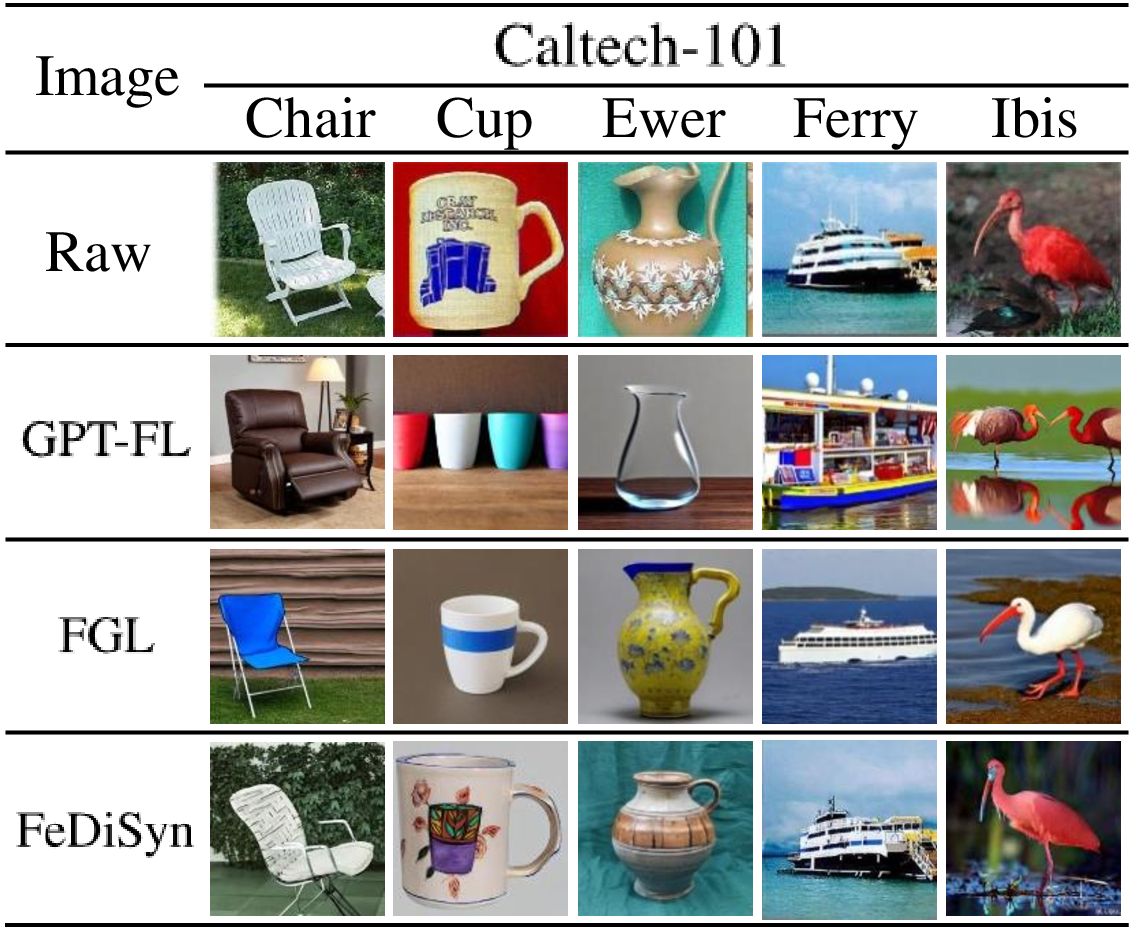
In contrast, FeDiSyn uploads latents encoding local data features to generate synthetic images, as elaborated in Section 3. For example, generated images for Caltech-101 li2004Learning? in Fig. 1 show that FeDiSyn can obtain synthetic images that better align with the feature distributions of raw data compared to GPT-FL and FGL.
2.2 Scaling Law of Synthetic-Image Pre-Training for FedFT↩︎
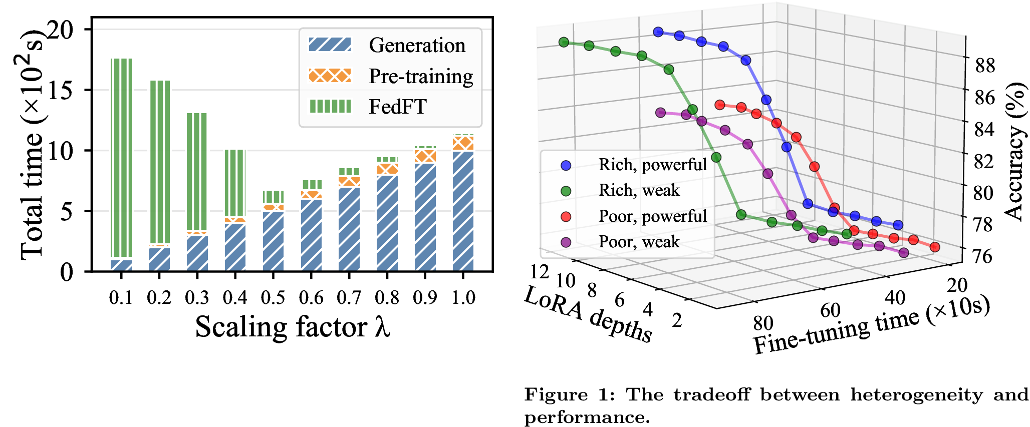
Following the groundbreaking success of large-scale models, scaling laws have emerged as a critical framework for quantifying the power-law relationships between model/data scale and performance kaplan2020scaling?. Prior studies have demonstrated that pre-training data volume has a significant impact on model performance zhang2024when?, pearce2024scaling?, which has motivated recent extensions of these principles to synthetic data, exploring how generative data scale influences convergence fan2024scaling?, kang2025demystifying?. However, these investigations focus exclusively on centralized training paradigms and are therefore not directly applicable to the FedFT setting, where the capabilities of servers for pre-training and edge devices for fine-tuning jointly determine the overall training time. As illustrated in Fig. 2 on Caltech-101, the synthetic scaling factor \(\lambda\) introduces a trade-off in FedFT: increasing \(\lambda\) accelerates convergence but incurs substantial overhead in image generation and pre-training. Therefore, the total completion time follows a U-shaped curve, which, in this example, attains its minimum near \(\lambda = 0.5\).
To provide guidance for synthetic pre-training in the FedFT setting, we propose a novel scaling law that quantifies the relationship between synthetic volume, target accuracy, and total training time, enabling the analytical determination of the optimal scaling factor \(\lambda\), as elaborated in Section 5.
2.3 Federated Fine-Tuning with LoRA for LVMs↩︎
LoRA hu2022lora? fine-tuning is a specific PEFT approach via low-rank matrix decomposition. In LoRA-based FedFT, each device only fine-tunes and uploads the lightweight inserted LoRA layers while keeping the pre-trained model frozen. The server aggregates the uploaded LoRA parameters and then distributes them back to all devices. Most existing LoRA-based FedFT approaches for LVMs wang2025federated?, su2024fedra? insert LoRA layers into all transformer layers, causing significant computation overhead. To reduce this burden, a few studies pfeiffer2024efficient?, liu2025adaptive? insert LoRA only to a subset of layers, enabling more efficient fine-tuning on resource-constrained devices. Futhermore, these works typically address system heterogeneity by assigning LoRA depths based solely on device capabilities: powerful devices receive deeper LoRA layers, while resource-constrained devices get smaller ones. However, weak devices may play a critical role in FedFT, and assigning them shallow LoRA depths can significantly degrade performance. We conduct a case study with ViT-B/16 fine-tuned on CIFAR-10 krizhevsky2009learning? in Fig. [fig:lora95tradeoff], which compares accuracy and fine-tuning time across four device types: (i) rich-data/powerful-capability, (ii) rich-data/weak-capability, (iii) poor-data/powerful-capability, and (iv) poor-data/weak-capability. As shown, powerful but data-scarce devices (red line) gain little benefit from deeper LoRA depths, whereas data-rich devices with weak-capability (green line) achieve accuracy comparable to powerful ones (blue line) when given a deeper LoRA, albeit with longer fine-tuning time. These observations highlight a trade-off: It is worth setting a larger LoRA depth for resource-constrained yet critical devices, but these devices may become stragglers that delay the overall FedFT process.
To this end, we propose a contribution-aware LoRA configuration and bandwidth allocation strategy in FeDiSyn. LoRA depth for each device is determined by its expected performance gain, while bandwidth is allocated to balance device completion times, effectively addressing system heterogeneity. Details are elaborated in Section 5.
3 System Design of FeDiSyn↩︎
3.1 Preliminaries↩︎
We consider a \(K\)-class classification problem performed through FedFT with label space \(\mathcal{C} = \{c_1, c_2, ..., c_K\}\). The system contains a centralized server with relatively abundant computational resources and a set of devices \(\mathcal{V} = \{v_1, v_2, ..., v_{N}\}\). Each device \(v_i\) owns a local dataset \(\mathcal{D}_i\), with size \(D_i=|\mathcal{D}_i|\). The global dataset across all devices is represented as \(\mathcal{D}\), with size \(D=|\mathcal{D}|= \sum_{v_i\in \mathcal{V}}D_i\). The data labeled as \(c_k\) on \(v_i\) is denoted as \(\mathcal{D}_i^k\) with size \(D_i^k=|\mathcal{D}_i^k|\), and it holds that \(\sum_{c_k\in\mathcal{C}}D_i^k = D_i\). The loss function of \(v_i\) is defined as \[\label{eq:filossfuction} f_i(\mathbf{w})\triangleq\tfrac{1}{D_i}\sum\nolimits_{\xi\in \mathcal{D}_i}f_i(\mathbf{w};\xi),\tag{1}\] where \(\mathbf{w}\) is the parameter vector, and \(f_i(\mathbf{w};\xi)\) is the loss over sample \(\xi\) in \(\mathcal{D}_i\). The global loss function on all the distributed datasets is \[\label{eq:lossfuction} F(\mathbf{w})\triangleq\sum\nolimits_{v_i\in \mathcal{V}}\tfrac{D_i}{D}f_i(\mathbf{w}).\tag{2}\] The learning problem is to find the optimal parameter vector \(\mathbf{w}^*\) so as to minimize \(F(\mathbf{w})\), i.e., \(\mathbf{w}^*=\mathop{\arg\min}_{\mathbf{w}} F(\mathbf{w})\).
3.2 System Overview↩︎
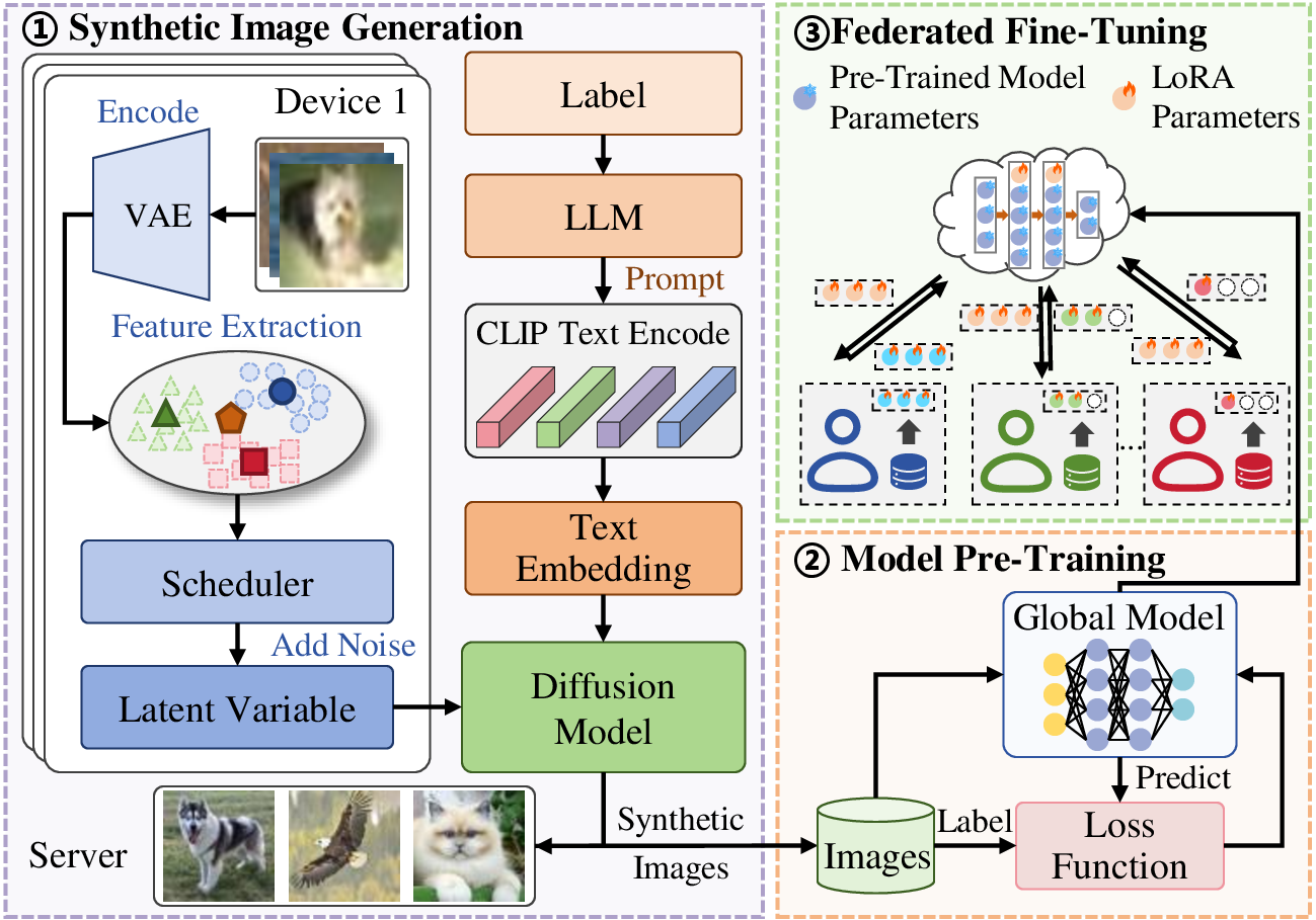
As shown in Fig. 3, the process of FeDiSyn consists of three steps. 1 Synthetic image generation: Devices encode private images into low-dimensional latents using a lightweight variational autoencoder (VAE). These latents are clustered to obtain class-specific centroids and a global average representation, which are then sent to the server with their labels. The server uses an large language model (LLM) to expand labels into diverse text prompts, encodes them via CLIP’s radford2021learning? text encoder, and feeds the resulting embeddings along with the uploaded latents into a DM (e.g., Stable Diffusion) to generate synthetic images, where latents govern stylistic features (e.g., lighting, texture) and text embeddings condition semantics (e.g., class-specific details). 2 Model pre-training: The server pre-trains a global model over synthetic images, yielding an initial model that captures cross-device features for subsequent FedFT. 3 Federated fine-tuning: The initialized model is sent to devices for LoRA-based fine-tuning under the FedFT framework. Specifically, each device keeps the pre-trained model frozen and updates only LoRA parameters, which are aggregated by the server and redistributed until convergence. The following sections detail each step.
3.3 Synthetic Image Generation↩︎
Data Feature Extraction. To align synthetic images with device-specific styles while preserving privacy, each device \(v_i\) extracts the features of its raw images locally in the latent space. Specifically, each sample \(\mathcal{D}_{i,j}^k\in \mathcal{D}_i^k\) of class \(c_k\) on device \(v_i\) is encoded by a VAE \(\mathcal{E}\) to obtain latents \(e_{i,j}^k=\mathcal{E}(\mathcal{D}_{i,j}^k)\). Subsequently, for the same class \(c_k\), device \(v_i\) clusters the latents \(e_{i,j}^k, \forall j\) into \(Z\) cluster centroids \(\mathbf{e}_{i,z}^k,z\in [1,Z]\), and calculate their average representation as \(\mathbf{e}_{i}^k\). \(\mathbf{e}_{i,z}^k\) and \(\mathbf{e}_{i}^k\) capture the style characteristics of the device distribution yang2024exploring?. Then the device uses a scheduler to add noise to the encoded latents at a randomly chosen diffusion timestep \(s\in\left\{0,...,S\right\}\) rombach2022high? as \[\label{eqn:addnosie} \begin{align} &\bar{\mathbf{e}}_{i,z}^{k,s}=\sqrt{\alpha_s}\mathbf{e}_{i,z}^k+\sqrt{1-\alpha_s}\epsilon, \epsilon\sim \mathcal{N}(0, I), z\in[1,Z], \\ &\bar{\mathbf{e}}_{i}^{k,s}=\sqrt{\alpha_s}\mathbf{e}_{i}^k+\sqrt{1-\alpha_s}\epsilon, \epsilon\sim \mathcal{N}(0, I), \end{align}\tag{3}\] where \(\alpha_s\) controls noise intensity at timestep \(s\). The device retains the raw data locally and only uploads the cluster centroids \(\bar{\mathbf{e}}_{i,z}^{k,S}\), the average representation \(\bar{\mathbf{e}}_{i}^{k,S}\), and its class label \(c_k\) to the server.
Label Collection and Prompt Engineering. The server collects the data volume \(D_i^k\) labeled as \(c_k\) of each device \(v_i\) and calculates the total amount of data labeled as \(c_k\) across all devices by \(D^k = \sum_{v_i \in \mathcal{V}} D_i^k\). To enrich semantic variety, a deployed LLM expands each label into multiple descriptive prompts. It has been verified that language enhancement is an effective way for enlarging synthetic image diversity for pre-training he2022synthetic?. For example, for the label “dog”, the prompt can be semantically expanded as follows:
Q: Write a sentence using the word “dog” to describe the characteristics and actions of the object.
A: A golden retriever playing on the grass.
These prompts are encoded into text embeddings via CLIP’s text encoder, ensuring semantic alignment between text and image latent spaces. To preserve the real data distribution, the synthetic image size for class \(c_k\) is set as \(\hat{D}^k = \lambda D^k\). \(\lambda\) is the scaling factor, which is determined according to our proposed scaling law in Section 5.
Synthetic Image Generated by Diffusion Model. On the server, for each class \(c_k\), the received cluster centroids \(\bar{\mathbf{e}}_{i,z}^{k,S}\) and average representation \(\bar{\mathbf{e}}_{i}^{k,S}\) are weighted as \(\bar{E}_{i,z}^{k,S}= \rho \bar{\mathbf{e}}_{i,z}^{k,S} + (1-\rho)\bar{\mathbf{e}}_{i}^{k,S}\), where \(\rho\) is a factor with a value between 0 and 1. Next, each latent \(\bar{E}_{i,z}^{k,S}\) is paired with a text embedding and fed into a latent DM, where latents guide stylistic consistency and text embeddings enforce data diversity. At each reverse step, a PNDM scheduler liu2022pseudo? is employed for sampling, iteratively denoising \(\bar{E}_{i,z}^{k,S}\) over \(S\) steps via \[\label{eqn:denosie} \phi(\bar{E}_{i,z}^{k,S},\epsilon_s,s,s-\delta)=\tfrac{\sqrt{\overline{\alpha}_{s-\delta}}}{\sqrt{\overline{\alpha}_s}}\bar{E}_{i,z}^{k,S} -\tfrac{(\overline{\alpha}_{s-\delta}-\overline{\alpha}_s)}{\sqrt{\overline{\alpha}_s}\left(\sqrt{(1-\overline{\alpha}_{s-\delta})\overline{\alpha}_s}+\sqrt{(1-\overline{\alpha}_s)\overline{\alpha}_{s-\delta}}\right)}\epsilon_s,\tag{4}\] where \(\delta\) is the step interval, and the gradient term \(\epsilon_s\) is computed using numerical methods such as the Runge-Kutta method or the linear multi-step method. Ultimately, all \(\bar{E}_{i,z}^{k,S}, \forall i,k\) undergo a certain number of denoising process to produce synthetic images \(\hat{\mathcal{D}}\) with size \(\hat{D}=\sum_{c_k\in\mathcal{C}}\hat{D}_k=\lambda\sum_{c_k\in\mathcal{C}} D_k\) at server side.
Remark 1 (Privacy Analysis). Transmitting latent representations is a widely used strategy for data augmentation in FL. Considering the limited amount of latent information uploaded by each device, our approach introduces minimal privacy leakage. Furthermore, similar to yang2024exploring?, we generate images using DM from noise-added features. As a result, even when the original images contain sensitive content (e.g., text or faces), the generated images exhibit entirely different semantic details. Therefore, despite potential visual similarities, they do not reveal or compromise the underlying private information.
3.4 Model Pre-Training over Synthetic Image↩︎
With the generated synthetic images \(\hat{\mathcal{D}}\) on the server, a global model is pre-trained in a standard supervised fashion. Similar to Eq. 2 , we denote \(\hat{F}(\mathbf{w})\) as the loss function over the synthetic images \(\hat{\mathcal{D}}\) for model parameters \(\mathbf{w}\). Starting from an initial parameter vector \(\hat{\mathbf{w}}^0\), the server performs \(\hat{T}\) iterations of model pre-training by \[\label{eqn:synloss} \hat{\mathbf{w}}^t=\hat{\mathbf{w}}^{t-1}-\eta\nabla\hat{F}(\hat{\mathbf{w}}^{t-1}),\tag{5}\] where \(\eta\) is the learning rate, and \(\nabla\) is the gradient operator. The global model after \(\hat{T}\) iterations of pre-training is denoted by \(\overline{\mathbf{w}}=\hat{\mathbf{w}}^{\hat{T}}\), which acts as the initial model for the subsequent FedFT process.
3.5 Federated Fine-Tuning with LoRA↩︎
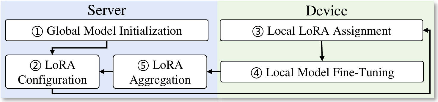
After the pre-training model \(\overline{\mathbf{w}}\) is obtained, FeDiSyn performs FedFT with LoRA for the LVM through the five phases shown in Fig. 4.
1 Global Model Initialization. The server first injects the LoRA layers into the pre-trained model \(\overline{\mathbf{w}}\), i.e., embedding initial LoRA matrices \(\widetilde{\mathbf{w}}^{0}=\{\widetilde{\mathbf{w}}_l^{0}, \forall l\in [0,L-1]\}\) within \(L\) transformer layers of the neural network. Then the embedded pre-trained model \(\mathbf{w}^0=\{\overline{\mathbf{w}}, \widetilde{\mathbf{w}}^0\}\) is distributed to all devices in \(\mathcal{V}\).
2 LoRA Configuration. Prior studies zhang2023adaptive?, liu2025adaptive? show that inserting LoRA into deeper layers yields better fine-tuning performance than shallow layers. Therefore, we define LoRA depth as the number of layers with LoRA modules, counted from the deepest output layer upward. At each round \(t\), the server assigns each device \(v_i\) a depth \(x_i^t\) based on its heterogeneous resources, thus only the last \(x_i^t\) layers \(L_i^t=\{l|L-x_i^t \le l < L\}\) are fine-tuned. The LoRA configuration strategy for all devices at round \(t\) is denoted as \(\mathcal{X}^t = \{x_i^t|v_i\in\mathcal{V}\}\), which will be described in Section 5.
3 Local LoRA Assignment. At each round \(t\), the server distributes the configuration information \(\mathcal{X}^t\) and the global LoRA parameters \(\widetilde{\mathbf{w}}^t=\{\widetilde{\mathbf{w}}_{l}^{t}| \forall l\in [0,L-1]\}\) to all devices in \(\mathcal{V}\). The \(l\)-th LoRA layer of device \(v_i\)’s local model is assigned as \[\label{eqn:update} \widetilde{\mathbf{w}}_{i,l}^{t}=\widetilde{\mathbf{w}}_l^{t}.\tag{6}\]
4 Local Model Fine-Tuning. After the local LoRA configuration, \(v_i\) fine-tunes the local model \(\mathbf{w}_i^t=\{\overline{\mathbf{w}}, \widetilde{\mathbf{w}}_i^t\}\) on its local dataset \(\mathcal{D}_i\). The update of each LoRA layer \(\widetilde{\mathbf{w}}_{i,l}^{t}\) at round \(t\) is expressed as \[\label{eqn:lora-fine-tuning} \begin{align} \widetilde{\mathbf{w}}_{i,l}^{t+1}= \begin{cases} \widetilde{\mathbf{w}}_{i,l}^{t}-\eta\nabla f_i(\widetilde{\mathbf{w}}_{i,l}^{t}), & L - x_i^t \le l < L \\ \widetilde{\mathbf{w}}_{i,l}^{t}, & otherwise \end{cases}. \end{align}\tag{7}\]
5 LoRA Aggregation. After local fine-tuning, each device \(v_i\) uploads the fine-tuned LoRA parameters \(\widetilde{\mathbf{w}}_{i,l}^{t+1}, L - x_i^t \le l < L\) to the server. Upon receiving the updated LoRA parameters from all devices, for each layer \(l\), the server aggregates them as \[\label{eqn:aggregation} \widetilde{\mathbf{w}}_l^{t+1}=\frac{\sum_{v_i\in\mathcal{V}}[l\ge L-x_i^t] D_i\widetilde{\mathbf{w}}_{i,l}^{t+1}}{\sum_{v_i\in\mathcal{V}}[l\ge L-x_i^t] D_i},\tag{8}\] where \([\cdot]\) is the Iverson notation. As a result, the global LoRA parameters are updated as \(\widetilde{\mathbf{w}}^{t+1}=\{\widetilde{\mathbf{w}}_{l}^{t+1}| \forall l\in [0,L-1]\}\), and the server configures LoRA for the next round \(t+1\). The process repeats until the model converges or reaches satisfactory accuracy.
4 Convergence Analysis↩︎
We make the following assumptions on the loss functions \(F(\mathbf{w})\) for convergence analysis, which are widely used in prior works wang2019adaptive?.
Assumption 1 (Lipschitz). The loss function \(F\) has a \(\mathcal{L}\)-Lispschitzian gradient for \(\forall \mathbf{w}_1,\mathbf{w}_2\), i.e., \(\|\nabla F(\mathbf{w}_1)-\nabla F(\mathbf{w}_2)\| \le \mathcal{L} \|\mathbf{w}_1-\mathbf{w}_2\|\).
Assumption 2 (Gradient Bounded). The expected squared norm of gradients is uniformly bounded for \(\forall\mathbf{w}_i^t\), i.e., \(\mathbb{E}\|\nabla F(\mathbf{w}_i^t)\|^2\le G^2\).
For LoRA fine-tuning, each LoRA matrix is further decomposed as \(\widetilde{\mathbf{w}}_i^{t}=\mathcal{B}_i^t\mathcal{A}_i^t, \forall i,t\), where \(\mathcal{B}_i^t\) and \(\mathcal{A}_i^t\) are low-rank matrices.
Assumption 3 (LoRA Bounded). There exist constants \(C_\mathcal{A},C_\mathcal{B}>0\), such that \(\|\mathcal{A}_i^t\|_2\le C_\mathcal{A}\), \(\|\mathcal{B}_i^t\|_2\le C_\mathcal{B}\).
Based on the above assumptions, we derive the convergence bound of FeDiSyn by the following theorem.
Theorem 1 (Convergence of FeDiSyn). After \(T\) rounds of fine-tuning in FeDiSyn, the expectation of the gradient of the LoRA matrices satisfies \[\begin{align} &\frac{1}{TN}\sum\nolimits_{t=1}^T\sum\nolimits_{v_i\in\mathcal{V}}\left(\mathbb{E}\|\nabla F(\mathcal{A}_i^t)\|^2+\mathbb{E}\|\nabla F(\mathcal{B}_i^t)\|^2\right)\notag\\&\le\frac{1}{N}\sum\nolimits_{v_i\in\mathcal{V}}\frac{\mathbb{E}[F(\mathbf{w}^0)]-\mathbb{E}[F(\mathbf{w}_i^{*})]}{\eta T}+\kappa, \end{align}\] where \(\mathbf{w}_i^*\) denotes the optimal model on \(v_i\), \(\kappa\) is a constant satisfying \([G^3C_\mathcal{A}C_\mathcal{B}+\frac{3\mathcal{L}}{2}(G^2C_\mathcal{A}^2+G^2C_\mathcal{B}^2+\eta^2G^4C_\mathcal{A}^2C_\mathcal{B}^2)]\eta+\frac{G^2}{2}\le\kappa\).
Due to limited space, we omit the proof of Theorem 1 here.
Remark 2 (LoRA-based FedFT Convergence). It is noticed that, unlike prior convergence analyses for FedFT liu2025adaptive?, wang2025federated?, which typically study the convergence behavior only at the level of the overall model parameter \(\mathbf{w}\), our analysis is developed specifically for LoRA-based FedFT and explicitly characterizes the convergence of the two low-rank matrices \(\mathcal{A}\) and \(\mathcal{B}\). As a result, our convergence bound provides a fine-grained theoretical understanding of the training in LoRA-based FedFT, and better reveals how the low-rank decomposition influences convergence.
5 Problem Formulation and Algorithm Description↩︎
5.1 Problem Formulation↩︎
The total completion time of FeDiSyn includes the image generation, pre-training, and FedFT time. Let \(\hat{h}\) denote the time to generate one image on server, then the total image generation time is expressed as \(H^{\rm gene}=\hat{D}\hat{h} =\lambda D\hat{h}\). Next, the server pre-trains LVM on synthetic data for \(\hat{T}\) rounds, and the pre-training time can be expressed as \(H^{\rm pre}=\lambda D \tilde{h}\hat{T}\), where \(\tilde{h}\) is the single round training time for one image on server.
For FedFT, although deeper LoRA layers improve its performance, practical deployments are constrained by resource limitations such as computation, communication, and memory. Let \(\overline{h}_i\) denote the time for data loading and performing a full forward pass through the LVM on \(v_i\) per sample, and \(h_i\) denote the additional time for backpropagating through per LoRA layer. Since the computation capacity of \(v_i\) is fixed, both \(\overline{h}_i\) and \(h_i\) can be measured in advance. Therefore, the fine-tuning time on device \(v_i\) at round \(t\) is given by \(H_i^{t, \rm comp}= D_i(\overline{h}_i + x_i^t h_i)\). The transmission time primarily arises from uploading LoRA parameters via FDMA, which allows simultaneous transmissions from multiple devices wang2025federated?. Let \(B_i^t\) denote the bandwidth allocated to \(v_i\) at round \(t\), then the uplink transmission rate \(r_i^t=B_i^t\log(1+\frac{p_ih_i^t}{\sigma^2})\) is modeled by the Shannon capacity, where \(p_i\) is the transmission power, \(h_i^t\) is the channel gain, and \(\sigma^2\) is the noise power. Therefore, the transmission time for \(v_i\) at round \(t\) is \(H_i^{t,\rm comm}=\tfrac{\tau x_i^t}{r_i^t}\), where \(\tau\) is the parameter size per LoRA layer. The duration of round \(t\) is determined by the slowest device, i.e., \[\label{eqn:max95time} H^t=\max\nolimits_{v_i \in\mathcal{V}}\{H_i^{t,\rm comp}+H_i^{t,\rm comm}\}.\tag{9}\]
For memory, let \(\overline{m}\) denote the fixed memory to load the LVM and store forward activations, and \(m\) represent the extra memory incurred by gradient storage per LoRA layer during backpropagation. Then, the total memory overhead for fine-tuning on \(v_i\) at round \(t\) is \[\label{eqn:memory} m_i^t = \overline{m} + x_i^t m.\tag{10}\]
Let the total completion time \(H=H^{\rm gene}+H^{\rm pre}+\sum\nolimits_{t=1}^T H^t\), we formulate the problem as follows: \[\begin{align} \boldsymbol{(P1)}:&\min\nolimits_{\lambda,\mathcal{X}^t,\mathcal{B}^t} H \\ {\boldsymbol{s.t.}} \quad &F(\mathbf{w}^T)-F(\mathbf{w}^*)\le \epsilon \tag{11}\\ & \sum\nolimits_{v_i\in\mathcal{V}} B_i^t \le B &\forall t\in[0,T] \tag{12}\\ & m_i^t \le M_i & \forall i\in [1,N] \tag{13} \end{align}\] Constraint 11 represents the global model converges after \(T\) rounds, where \(\epsilon\) is the convergence threshold. Constraint 12 ensures the total allocated bandwidth does not exceed the budget \(B\) in each round. Constraint 13 ensures each device \(v_i\)’s memory usage does not exceed its available memory \(M_i\). Our objective is to decide the data scaling factor \(\lambda\), the LoRA depth configuration \(\mathcal{X}^t=\{x_i^t|v_i\in\mathcal{V}\}\) and bandwidth allocation \(\mathcal{B}^t=\{B_i^t|v_i\in\mathcal{V}\}\) for each round, minimizing the total completion time, i.e., \(\min_{\lambda,\mathcal{X}^t,\mathcal{B}^t}H\).
5.2 Algorithm Description↩︎
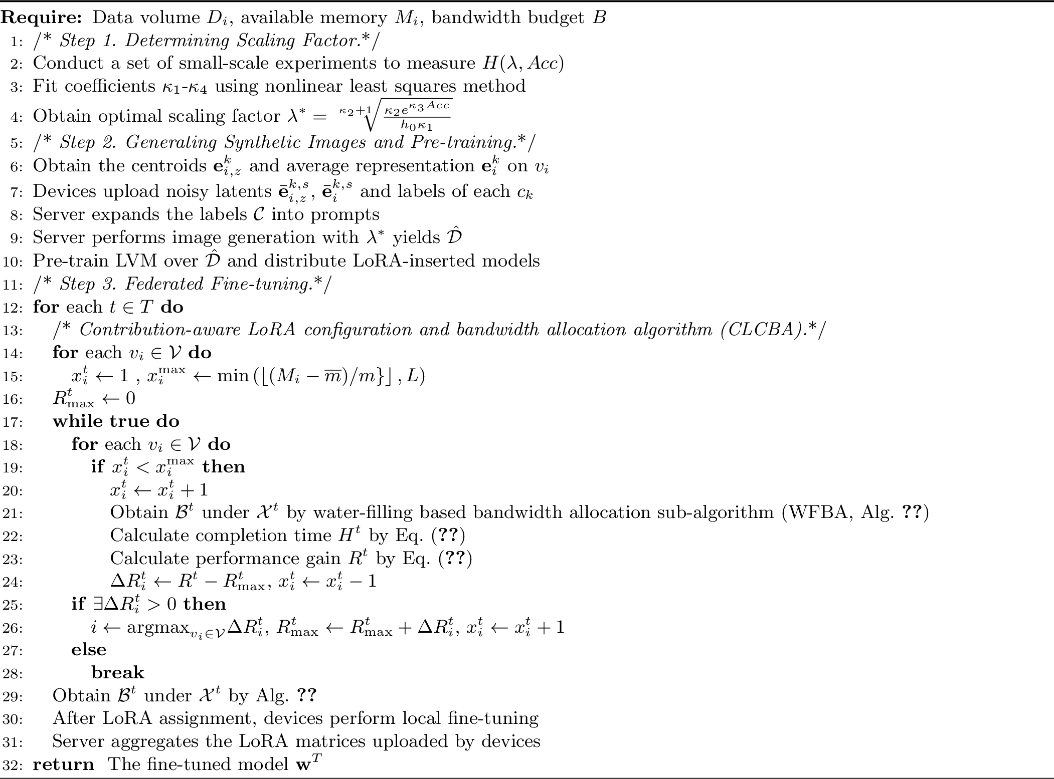
In this section, we introduce the algorithm description for our FeDiSyn to solve problem P1, as described in Alg. 5.
1 Determining Scaling Factor. The key challenge of solving problem P1 is determining the scaling factor \(\lambda\) to balance the time required for synthetic image generation/pre-training and FedFT. From Section 5.1, the total time for generation and pre-training is \(H^{\rm gene}+H^{\rm pre}=\lambda D\hat{h}+\lambda D \tilde{h}\hat{T}=\lambda(\hat{h}+\tilde{h}\hat{T})D=\lambda h_0\), where \(h_0\triangleq(\hat{h}+\tilde{h}\hat{T})D\) is defined as the unit time for generation and pre-training. Conversely, empirical analysis across multiple datasets suggests that the subsequent FedFT time is negatively correlated with \(\lambda\) and grows exponentially with the target accuracy \(Acc\). To quantify this relationship, we propose the following scaling law to describe the total completion time as \[\label{eqn:time95lambda95acc} H(\lambda, Acc)=h_0\lambda +\tfrac{1}{\kappa_1\lambda^{\kappa_2}}e^{\kappa_3 Acc}+\kappa_4,\tag{14}\] where \(h_0 \lambda\) represents the linear growth of generation and pre-training time, and the remaining terms capture the diminishing returns of synthetic data on FedFT acceleration. The architecture-specific coefficients \(\kappa_1\)-\(\kappa_4\), which depend on the dataset, model and device capacity, can be estimated in a short calibration phase using a set of small-scale pilot runs, detailed in Section 6.2. To find the optimal scaling factor \(\lambda^*\) that minimizes the total training time, we take the derivative of Eq. 14 with respect to \(\lambda\) as \(H'_{\lambda}=h_0-\tfrac{\kappa_2}{\kappa_1\lambda^{\kappa_2+1}}e^{\kappa_3 Acc}\). Taking \(H'_{\lambda}=0\) yields the optimal scaling factor \(\lambda^*=\sqrt[\kappa_2 + 1]{\tfrac{\kappa_2e^{\kappa_3 Acc}}{h_0\kappa_1}}\). We derive the following key insights regarding \(\lambda^*\).
Remark 3 (Impact of Server Capability). As the server’s computational capacity increases (\(h_0 \to 0\)), the optimal scaling factor \(\lambda^*\) grows. When the server possesses plenty of computational capacity, it can rapidly generate a vast synthetic images. As a result, a larger \(\lambda\) accelerates FedFT without incurring a significant generation time.
Remark 4 (Impact of Target Accuracy). The presence of \(Acc\) in the exponent, \(\lambda^* \propto e^{\tfrac{\kappa_3}{\kappa_2 + 1} Acc}\), reveals that the demand for synthetic data grows exponentially with the target accuracy. For low-accuracy requirements, the overhead of large-scale synthesis outweighs its benefits. However, for high-accuracy requirements, the FedFT time increases so sharply that a massive synthetic pre-training for model initialization becomes essential to reduce the total training time.
2 Generating Synthetic Images and Pre-Training.
After the optimal \(\lambda^*\) is determined, the server generates a corresponding number of synthetic images (Alg. 5, Lines [alg1:cluster]-[alg1:generation]) and pre-trains the LVM on the generated images dataset, then distributes LoRA-inserted model to devices (Alg. 5, Lines [alg1:pre-train]), as described in Section 3.3 and 3.4.
3 Federated Fine-Tuning. The main idea of FedFT is to determine the LoRA configuration \(\mathcal{X}^t\) to maximize the performance gain, while balancing completion times across devices through a bandwidth allocation strategy \(\mathcal{B}^t\). To handle device heterogeneity in FedFT, we design a contribution-aware LoRA configuration and bandwidth allocation (CLCBA) algorithm (Alg. 5, Lines [alg1:begin32t]-[alg1:end32t]). Since the local gradient \(g_i(\widetilde{\mathbf{w}}_{i,l}^t)=\nabla f_{i}(\widetilde{\mathbf{w}}_{i,l}^{t})\) captures the contribution of \(l\)-th layer to the loss function sun2025exploring?, li2025fedquad?, we use the L2 norm \(G_i^t = \sum_{l \in L_i^t}||g_i(\widetilde{\mathbf{w}}_{i,l}^{t-1})||_2^2\) of the last round \(t-1\) to quantify the contribution of \(v_i\) at round \(t\). The performance gain is defined as the sum of all devices’ contributions divided by current round’s duration \[\label{eqn:reward} R^t\triangleq\tfrac{\sum_{v_i\in\mathcal{V}} G_i^t}{H^t}=\tfrac{\sum_{v_i\in\mathcal{V}}\sum_{l \in L_i^t}||g_i(\widetilde{\mathbf{w}}_{i,l}^{t-1})||_2^2}{H^t}.\tag{15}\]
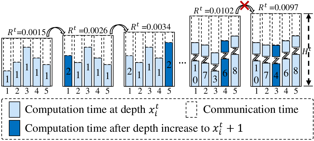
We first initialize the depths of all devices as 1, i.e., set \(x_i^t = 1\) for all \(v_i\in\mathcal{V}\) (Line [alg1:set32x95max]). In each iteration, we choose a device that obtains the maximum performance gain among all devices to add one LoRA layer. This process continues until the maximum performance gain is less than its value in the last iteration (Alg. 5, Line [alg1:begin32while]-[alg1:end32while]). Meanwhile, in each iteration of the process of Alg. 5, we call the water-filling based bandwidth allocation sub-algorithm (WFBA) to balance completion times across devices, which minimizes the completion time \(H^t\) in Eq. 15 .

The WFBA sub-algorithm is shown in Alg. 6. First, WFBA calculates the maximum computation time \(H_{\max}^{t, \rm comp}\) of all devices (Alg. 6, Lines [alg2:begin32initial]-[alg2:max32time]). Since the waterline must exceed the maximum computation time \(H_{\max}^{t, \rm comp}\), WFBA initializes the waterline as \(\mathcal{H}_0^t = 2 H_{\max}^{t, \rm comp}\) and iteratively solve its optimal value using Newton’s method more1982newton? (Alg. 6, Lines [alg2:begin32newton]-[alg2:end32newton]). Finally, WFBA calculates the optimal bandwidth allocation \(B_i^t\) for each device \(v_i\) based on the converged waterline and returns the bandwidth configuration \(\mathcal{B}^t\) (Alg. 6, Lines [alg2:begin32return]-[alg2:end32return]). The intuitive diagram of CLCBA to obtain \(\mathcal{X}^t\) and \(\mathcal{B}^t\) are shown in Fig. 7.
6 Performance Evaluation↩︎
6.1 System Setup↩︎
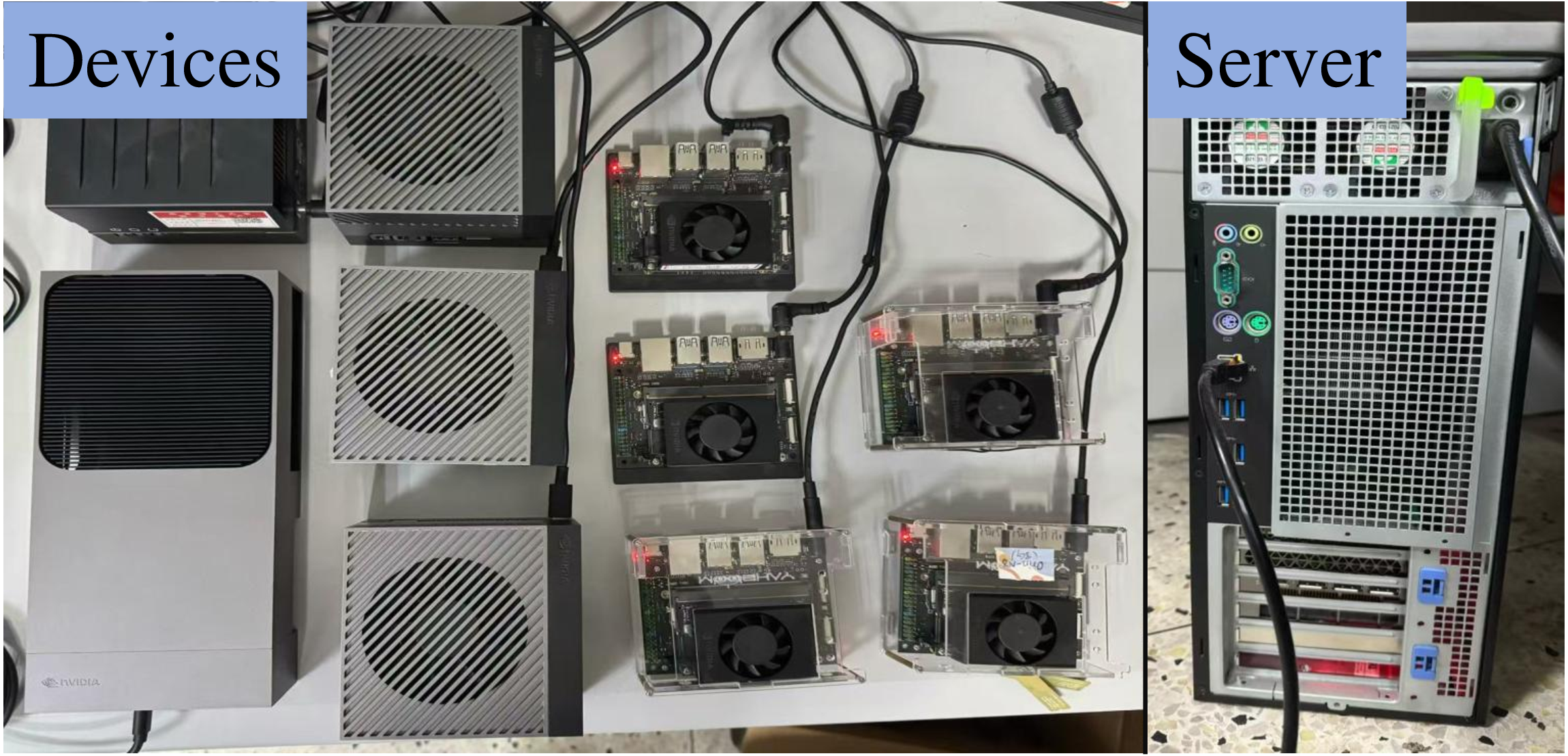
Environment Settings. We implement a FedFT experimental testbed comprising one server and 10 heterogeneous devices, as shown in Fig. 8. The server is equipped with an NVIDIA GeForce RTX 4090 GPU with 48GB GDDR6X. We use 1 Jetson AGX Xavier kit, 5 Jetson Orin NX kits, 3 Jetson AGX Orin kits, and 1 Jetson AGX Thor kit as heterogeneous devices. Particularly, we simulate more practical wireless communication in an edge environment instead of high-bandwidth laboratory networks, where communication time is typically negligible compared to computation time. Similar to wang2025federated?, the server is at (0, 0), and each device is uniformly distributed within a circular area of 50 meters radius centered at coordinates \((300,0)\). The large-scale fading is represented as \(\left( d/d_{0} \right)^{-3.5}\), where \(d_{0} = 10\) meters is the reference distance. The noise power is set as \(\sigma^2=10^{-11}\)W, with a total system bandwidth of \(B = 10\)MHz.
Models and Datasets. We train ViT-B/16 dosovitskiy2020image? on CIFAR-10 krizhevsky2009learning? and Caltech-101 li2004Learning? datasets, and train ViT-L/16 dosovitskiy2020image? on Food-101 bossard14food? dataset. ViT-B/16 and ViT-L/16 consist of 86 and 307 million parameters, respectively.
CIFAR-10 krizhevsky2009learning? is composed of 60,000 color images, which are divided into 10 classes, each containing 6,000 images. The dataset is further split into 50,000 training images and 10,000 test images.
Caltech-101 li2004Learning? comprises 101 classes objects, totaling 9,144 samples. The number of samples per category ranges from 40 to 800 images, with each category averaging approximately 50 samples. We divide it into a 4:1 training-test split ratio.
Food-101 bossard14food? contains a series of food datasets divided into 101 classes with high inter-class similarity. It comprises 101,000 samples, with each class including 750 training and 250 test samples.
We analyze FedFT performance under both IID and non-IID data among devices. For the non-IID data case, we adopt the Dirichlet distribution tzu2019measuring? with \(\alpha_{\rm dir}=0.3\) to partition the dataset. In addition, we deploy the LLaMa-7B touvron2023llama? to enrich prompts and Stable-Diffusion-v1-5 rombach2022high? to generate synthetic images as described in Section 3.3.
Benchmarks. We compare FeDiSyn against two solutions with synthetic image pre-training (GPT-FL zhang2025gpt?, FGL zhang2023federated?) and two solutions deploying LoRA-based FedFT (SFLF wang2025federated?, CAFF pfeiffer2024efficient?). Specifically, GPT-FL and FGL generate images based on uploaded labels or text embeddings from devices, while SFLF and CAFF determine each device’s LoRA depth based on its capacity. For a fair comparison, FeDiSyn, SFLF, and CAFF adopt the same LoRA rank.
GPT-FLzhang2025gpt? is a synthetic image pre-training based approach that expands device-uploaded labels into prompts and generates images for pre-training LVM, while using FedAvg mcmahan2017communication? for FedFT.
FGLzhang2023federated? is a synthetic image pre-training based approach where devices use BLIP to generate prompts for local images, and the server employs these prompts to generate images for pre-training LVM, while utilizing FedAvg for FedFT.
SFLFwang2025federated? is a LoRA-based approach for FedFT, where the LVM is initialized with ImageNet parameters, and all devices fine-tune all transformer layers of the LVM.
CAFFpfeiffer2024efficient? is an advanced LoRA-based approach that initializes LVM with ImageNet parameters, and assigns appropriate LoRA depths to each device to address system heterogeneity.
6.2 Evaluation Results↩︎


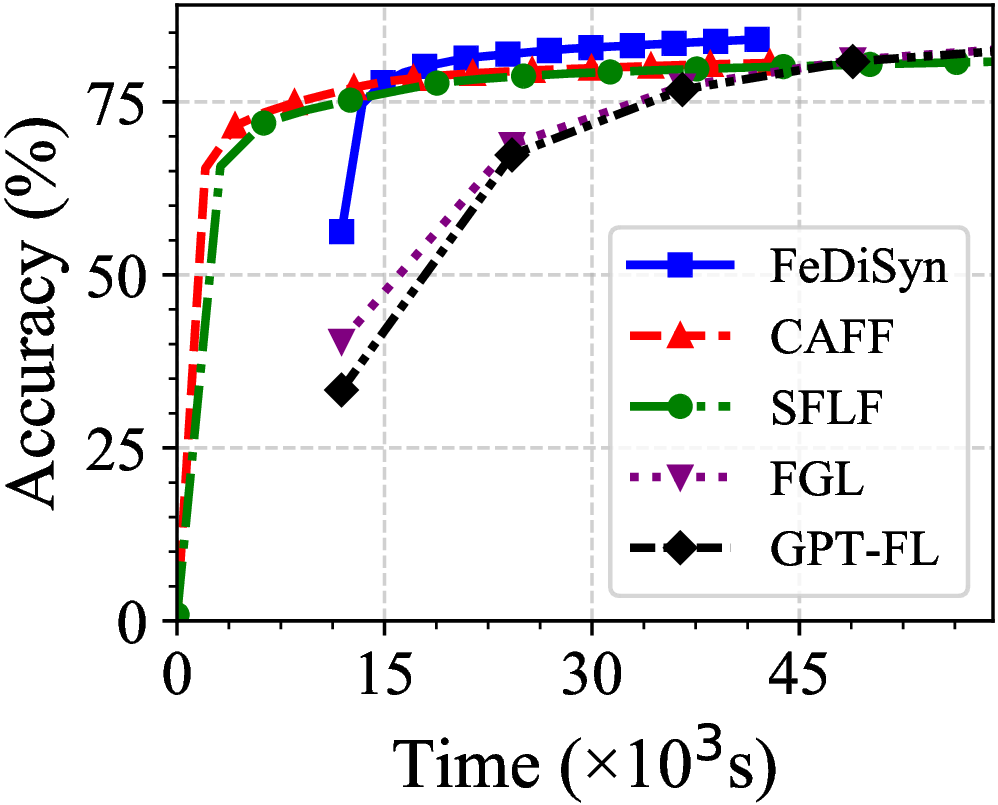
Figure 9: The test accuracy over different datasets (IID). Left: CIFAR-10; Middle: Caltech-101; Right: Food-101..


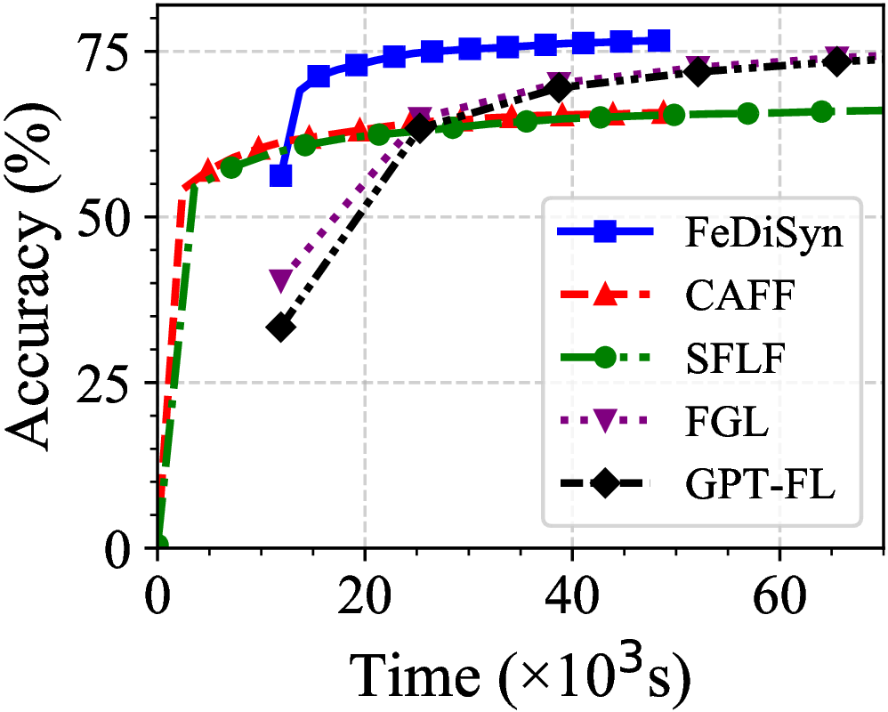
Figure 10: The test accuracy over different datasets (non-IID). Left: CIFAR-10; Middle: Caltech-101; Right: Food-101..


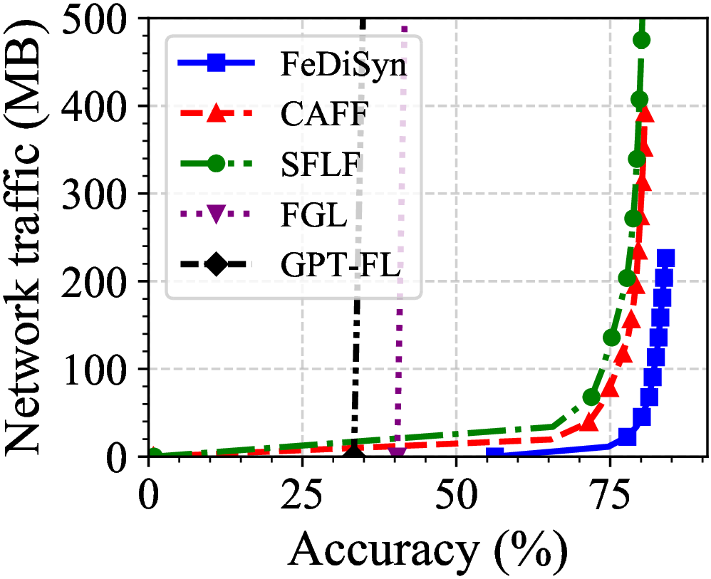
Figure 11: The network traffic over different datasets (IID). Left: CIFAR-10; Middle: Caltech-101; Right: Food-101..


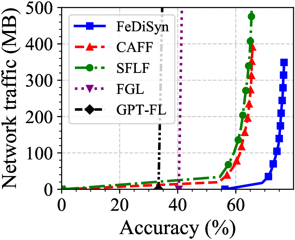
Figure 12: The network traffic over different datasets (non-IID). Left: CIFAR-10; Middle: Caltech-101; Right: Food-101..
Training Performance. We evaluate the FedFT process of our FeDiSyn method and the benchmarks on the CIFAR-10, Caltech-101 and Food-101 datasets under both IID and non-IID data distributions, as illustrated in Figs. 9 and 10. Overall, FeDiSyn consistently achieves the fastest convergence and highest accuracy on all datasets under both IID and non-IID data. For example, as shown in the third plot of Fig. 9, under IID data on Food-101, FeDiSyn reaches 80% accuracy in 17,584s, while CAFF, SFLF, FGL, and GPT-FL require 31,905s, 41,885s, 44,783s, and 45,383s, respectively, meaning FeDiSyn reduces 44.9%, 58.0%, 60.7%, and 61.3% completion time compared to these benchmarks. Moreover, under non-IID data, FeDiSyn’s advantage becomes even more pronounced compared to other solutions. As shown in the third plot of Fig. 10, under non-IID data, FeDiSyn reduces 62.0%, 70.5%, 52.5%, and 56.2% time for reaching 65% accuracy compared to CAFF, SFLF, FGL, and GPT-FL, respectively. This is because FeDiSyn pre-training over synthetic images that enhances the generalization ability of initial model, alleviating the impact of non-IID data jhunjhunwala2025initialization?.
Network Traffic Consumption. In Fig. 11 and 12, we compare the network traffic consumption by different solutions to achieve certain accuracies on CIFAR-10 Caltech-101 and Food-101, respectively. By the results, FeDiSyn significantly reduces the network traffic compared with the benchmarks. For example, under non-IID data on Food-101, the consumed network traffic of FeDiSyn, CAFF, SFLF, FGL, and GPT-FL is 7.4MB, 262.1MB, 399.5MB, 12,002.8MB, and 13,676.3MB, respectively. FeDiSyn can reduce network traffic by 97.2%, 98.1%, 99.9%, and 99.9% compared with these methods. Compared with the LoRA-based methods CAFF and SFLF, FeDiSyn adopts a more efficient LoRA configuration strategy, thereby reducing network traffic when achieving the target accuracy. In addition, FGL and GPT-FL rely on full parameter FedFT, which incurs extremely high communication overhead.
The complete experimental results of FedFT performance and network traffic consumption are provided in Table ¿tbl:tbl:overall95test?.
c|c|cccc>cc Dataset & Metric & GPT-FL & FGL & SFLF & CAFF & FeDiSyn
& Time & 232.5 & 220.3 & 103.5 & 73.3 & 55.1
& Traffic & 23243.5 & 21798.8 & 172.7 & 99.8 & 50.3
& Time & 348.6 & 341.3 & 203.7 & 161.1 & 92.3
& Traffic & 31051.5 & 29840.5 & 254.0 & 146.0 & 93.5
& Time & 113.7 & 96.4 & 14.6 & 10.3 & 6.8
& Traffic & 14547.6 & 12198.6 & 226.2 & 150.1 & 15.7
& Time & 147.5 & 116.7 & 18.9 & 14.5 & 6.3
& Traffic & 18564.2 & 14755.1 & 279.5 & 177.8 & 10.1
& Time & 453.8 & 447.8 & 418.9 & 319.1 & 175.8
& Traffic & 30763.4 & 30375.9 & 457.3 & 290.1 & 42.5
& Time & 284.9 & 262.2 & 423.1 & 328.4 & 124.7
& Traffic & 13676.3 & 12002.8 & 399.5 & 262.1 & 7.4
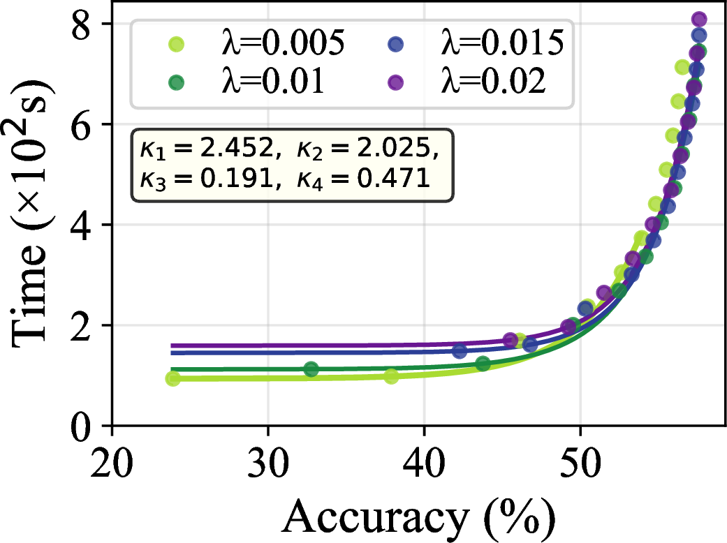
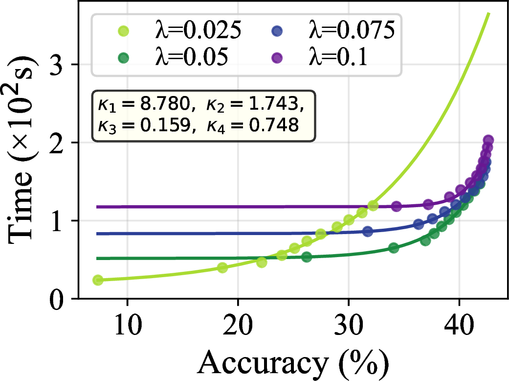
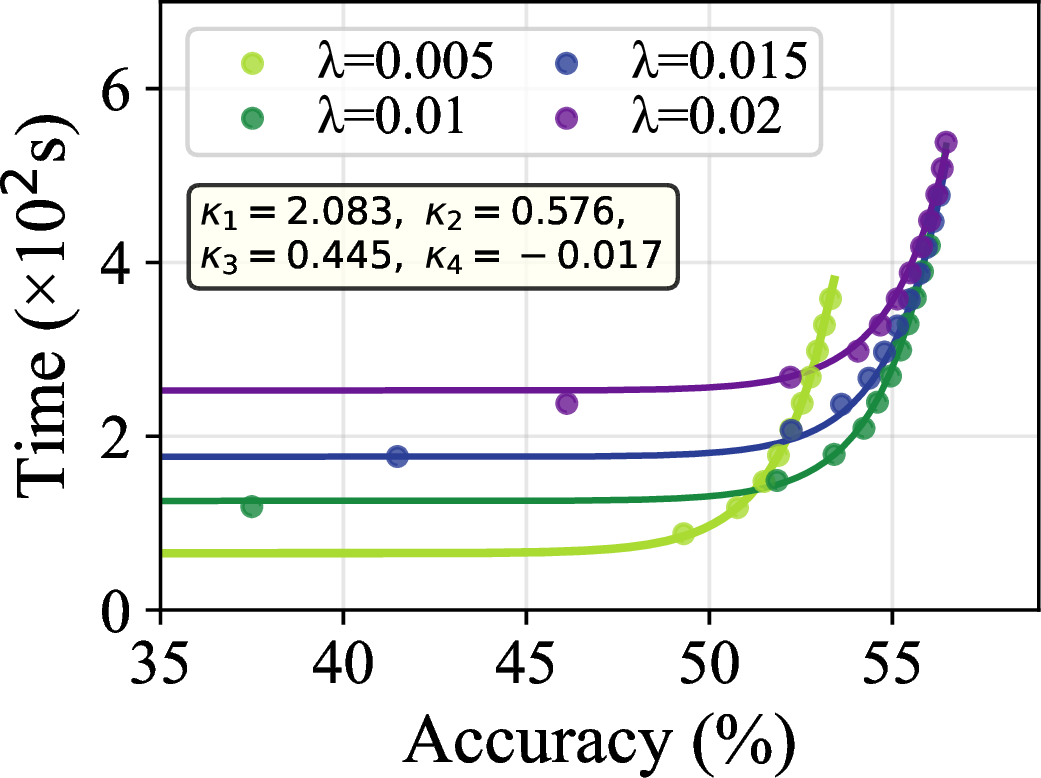
Figure 13: Fitting Eq. 14 with small \(\lambda\). Left: CIFAR-10; Middle: Caltech-101; Right: Food-101..
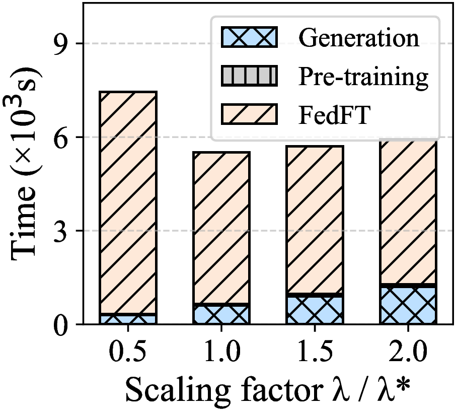
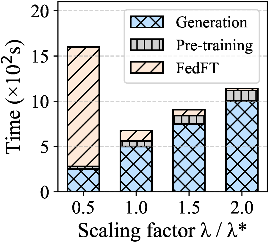
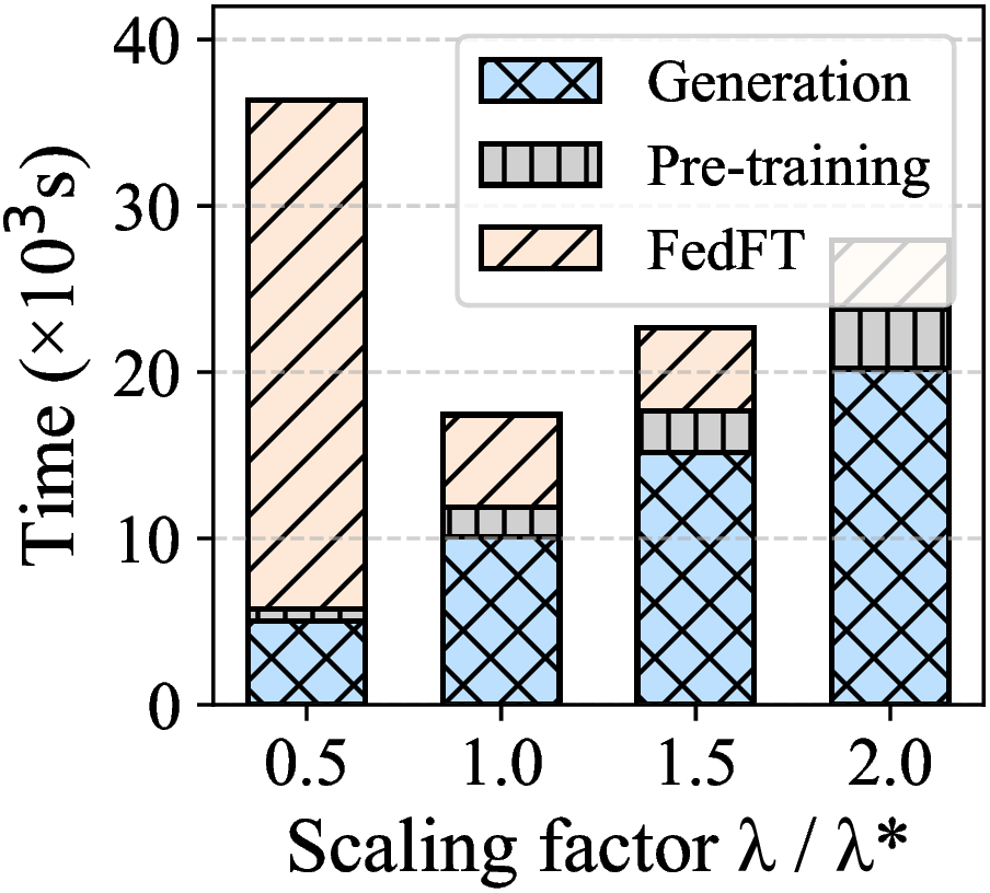
Figure 14: The time to reach target accuracy under different scaling factor \(\lambda\). Left: CIFAR-10 (85%); Middle: Caltech-101 (70%); Right: Food-101 (75%)..
Impact of Synthetic Image Volume. To estimate the values of coefficients \(\kappa_1-\kappa_4\) in Eq. 14 , we fit this equation in a short calibration phase using a set of small values of \(\lambda\) via nonlinear least-squares (e.g., Levenberg-Marquardt method). Fig. 13 shows that Eq. 14 well describes the relationship among total training time, accuracy and the volume of generated data. Then we obtain the optimal \(\lambda^*=\sqrt[\kappa_2 + 1]{\tfrac{\kappa_2e^{\kappa_3 Acc}}{h_0\kappa_1}}\) by the estimated coefficients.
Fig. 14 shows the time to reach target accuracy under different scaling factor \(\lambda=0.5\lambda^*, \lambda^*, 1.5\lambda^*\) and \(2\lambda^*\) on CIFAR-10, Caltech-101 and Food-101. \(Acc\) is set as 85%, 70% and 80% for CIFAR-10, Caltech-101 and Food-101, respectively. We observe that the generation and pre-training time increase linearly with \(\lambda\). For example, for Food-101, the generation times are 5,050s, 10,100s, 15,150s, and 20,200s for \(\lambda=0.5\lambda^*, \lambda^*, 1.5\lambda^*\), and \(2\lambda^*\), respectively. However, when the value of \(\lambda\) is too large or too small, the total completion time to achieve the target accuracy will be relatively long. For example, for Food-101, when \(\lambda\) increases from \(0.5\lambda^*\) to \(2\lambda^*\), the time required to achieve 80% accuracy is 36,351.0s, 17,583.9s, 22,671.1s, and 27,943.9s, respectively. This is because insufficiently generated images weaken pre-training effectiveness for FedFT, whereas excessive images introduce substantial computational overhead, thereby prolonging image generation. The experimental results in Figs. 13-14 show that the values of \(\lambda^*\) obtained by the empirical model have the shortest completion time compared to other values.
Ablation Study. FeDiSyn comprises two primary modules: 1) a feature-guided (FG) synthetic generation module with a diffusion model (DM), 2) a LoRA-based FedFT module deploying contribution-aware LoRA configuration (CLC) and water-filling bandwidth allocation (WFBA). We conduct fine-grained ablation experiments on CIFAR-10, Caltech-101, and Food-101 in Figs. 15 and 16 to evaluate the individual contribution of each sub-module. FeDiSyn consistently outperforms all variants, including those without FG, CLC, WFBA, or those utilizing GANs instead of DMs. For example, on CIFAR-10, FeDiSyn achieves 74% accuracy with 42.4%, 61.4%, 22.8%, and 41.7% time reduction and reduces network traffic usage by 47.0%, 65.6%, 12.5%, and 51.7%, compared to FeDiSyn w/o FG, FeDiSyn w/o DM, FeDiSyn w/o CLC, and FeDiSyn w/o WFBA, respectively. We also observe that the relative importance of synthetic pre-training grows with model scale. For example, for ViT-B/16 training on CIFAR-10 and Caltech-101, the performance gaps among different variants are relatively small, but for ViT-L/16 training on Food-101, FeDiSyn w/o CLC and w/o WFBA significantly outperform FeDiSyn w/o FG and w/o DM, even approaching the performance of FeDiSyn. This is because larger models possess a higher degree of representational complexity, making a high-quality pre-training for initialization far more critical than fine-tuning stage.
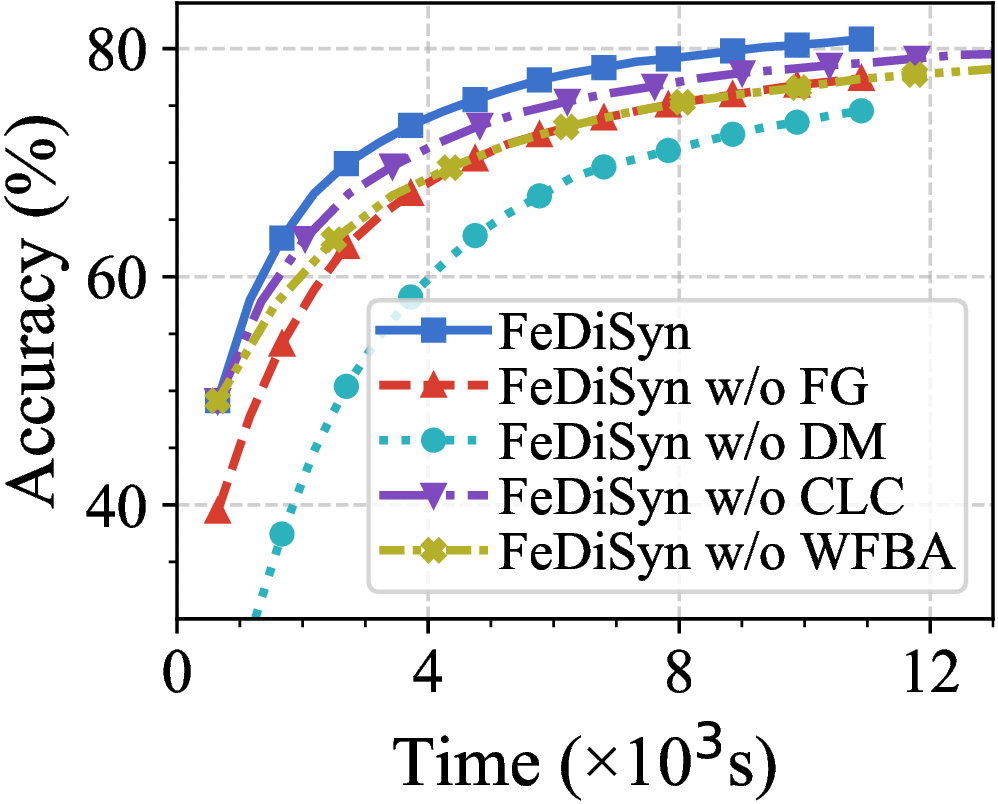
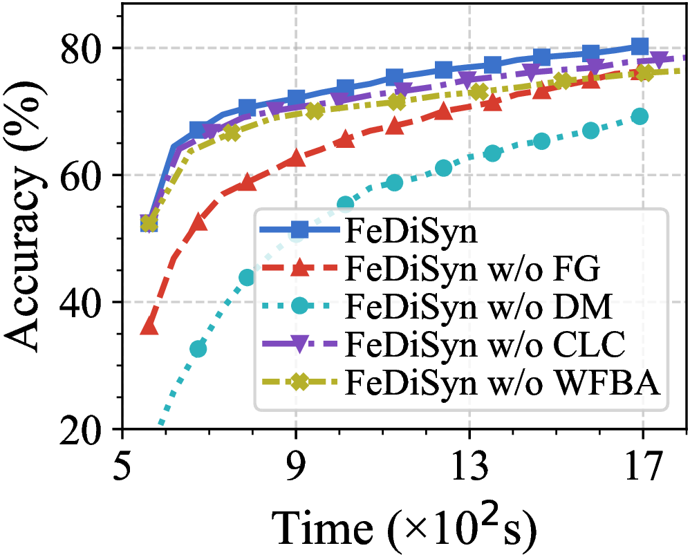
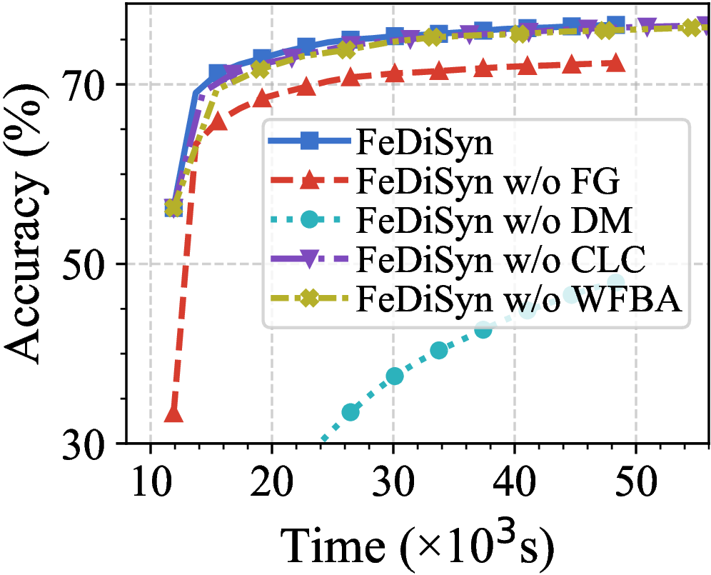
Figure 15: Ablation study on accuracy. Left: CIFAR-10; Middle: Caltech-101; Right: Food-101..
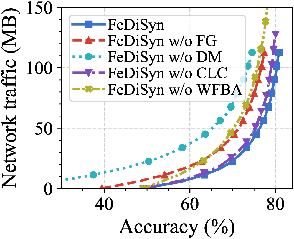
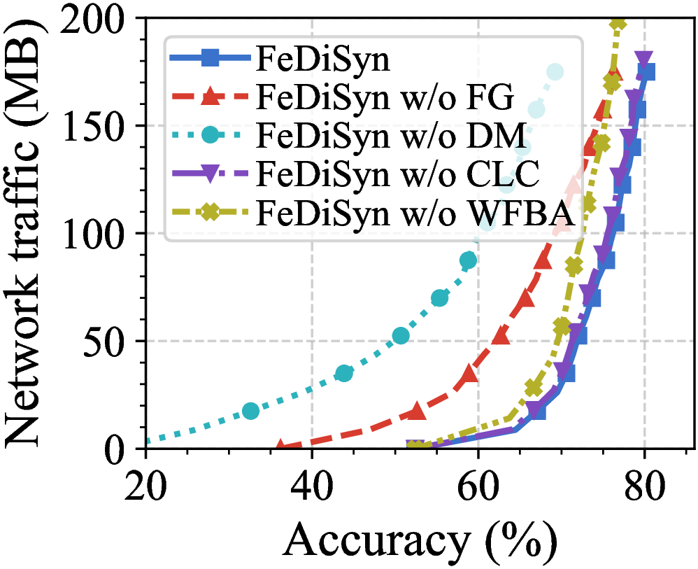
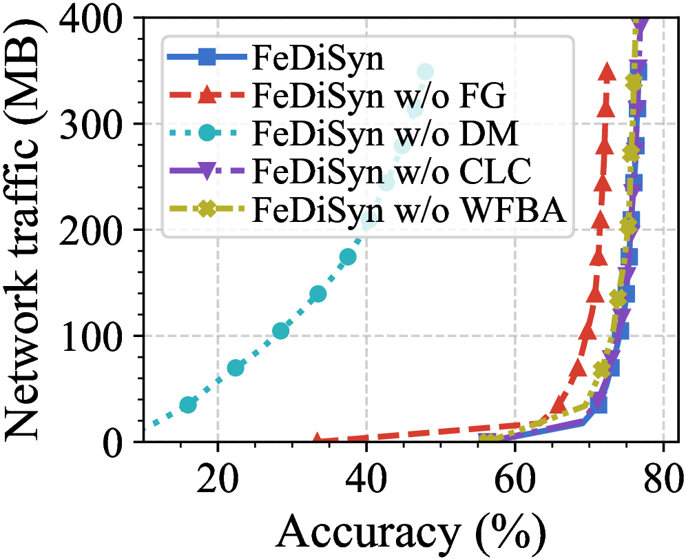
Figure 16: Ablation study on Bandwidth. Left: CIFAR-10; Middle: Caltech-101; Right: Food-101..
7 Conclusion↩︎
In this paper, we propose FeDiSyn, a unified framework that holistically considers both pre-training and federated fine-tuning (FedFT) of large vision models to address resource constraints, system heterogeneity, and non-IID data. FeDiSyn introduces a scaling law for synthetic pre-training under FedFT setting to determine the optimal number of synthetic images. A diffusion model is deployed on the server to generate synthetic images that align with the device’s local image label and feature distributions, thereby efficiently pre-training a superior initial global model for FedFT. During FedFT, we design a contribution-aware LoRA configuration and bandwidth allocation algorithm to enhance FedFT performance while addressing system heterogeneity. Experimental results indicate the superiority of our proposed framework compared with state-of-the-art solutions.
The corresponding author of this paper is Junlong Zhou. This work was supported in part by the National Science Foundation of China (NSFC) under Grants 62402537, 62572244, 62402226 and U25A20442, in part by the Natural Science Foundation of Jiangsu Province under Grant BK20241453, and in part by the Fundamental Research Funds for the Central Universities under Grant 30925010408.