A 2.5D NURBS-Trace Infinite-Element Method for Moving-Load Wave Propagation and Soil–Structure Interaction in Semi-Infinite Ground
July 14, 2026
Abstract
For moving-load problems with geometry and material properties that are approximately invariant along the traveling direction, 2.5D analysis retains three displacement components at substantially lower cost than full three-dimensional discretization. This paper presents a 2.5D Non-Uniform Rational B-spline (NURBS)-trace infinite-element method (NBIEM), formulated as a coupled finite/infinite-element scheme, for wave propagation in linear viscoelastic semi-infinite geotechnical media. The bounded near field is discretized by isogeometric analysis, whereas the exterior is represented by tensor products of the boundary NURBS basis and admissible outgoing or evanescent exponential radial functions. The two subdomains share the same discrete NURBS trace space and boundary control-point degrees of freedom, enforcing displacement continuity without projection or mortar variables. For the selected radial functions, the far-field stiffness and mass contributions are evaluated through closed-form radial moments, avoiding finite radial cutoff and radial quadrature. Closed-form half-space solutions verify displacement and stress frequency-response functions across sub-Rayleigh, super-shear but sub-compressional, and super-compressional moving-load regimes. Low-frequency studies assess the sensitivity of the selected exterior setting to radial parameters and artificial-boundary placement. Additional tests characterize complex-valued response accuracy, phase fidelity, computational cost, and the frequency-dependent working range of the default S-wave-informed exterior realization. Applications to layered media, track–subgrade systems, and buried structures demonstrate the method’s ability to handle heterogeneous materials, multi-patch configurations, curved interfaces, and cover-depth-dependent geotechnical responses. The resulting framework provides a geometrically consistent and computationally efficient treatment of moving-load wave propagation and soil–structure interaction in semi-infinite domains.
NURBS-trace infinite element ,2.5D viscoelastic wave propagation ,Moving loads ,Unbounded media ,Isogeometric analysis ,Radiation condition
1 Introduction↩︎
Ground vibration induced by moving loads is a persistent concern in transportation geotechnics and underground infrastructure engineering. Waves generated by high-speed trains, metro systems, heavy road traffic, and moving machinery can propagate through semi-infinite ground and affect the serviceability of adjacent buildings, sensitive facilities, pipelines, tunnels, and other buried structures. Field measurements have documented railway-induced ground vibration in operating lines [1], [2]. Road-traffic-induced ground vibration has been investigated through coupled vehicle–road and ground-response models [3]. Underground-railway vibration and its transmission through the surrounding ground have also been examined numerically and analytically [4], [5]. For tunnels embedded in layered ground, analytical and theoretical models have clarified the effects of stratification, tunnel geometry, and moving excitation [6], [7].
Reliable prediction is therefore needed at the design and assessment stages. The modeling task is demanding because the response is intrinsically three-dimensional, whereas the ground domain is unbounded and must satisfy radiation conditions at infinity. For systems that are approximately invariant along the traveling direction, the 2.5D formulation provides an effective compromise between full three-dimensional discretization and overly restrictive two-dimensional plane-strain models. By applying a Fourier transform along the longitudinal direction, the moving-load problem is reduced to a sequence of two-dimensional cross-sectional problems in the wavenumber–frequency domain. Analytical formulations based on transfer matrices and cylindrical-to-plane wave transformations provide efficient solutions for circular tunnels in horizontally layered half-spaces [6]. Related layered-ground models have also been developed for tunnel systems subjected to underground moving loads [7]. Their geometric and material assumptions, however, differ from those of general cross-sectional discretizations.
The treatment of the unbounded exterior domain is a central issue in 2.5D numerical modeling. In classical finite/infinite-element formulations, the near field is modeled by finite elements and the far field by infinite elements containing wave-propagation and decay functions [8]. This construction is compact, but its accuracy depends on the selected radial approximation and on a finite/infinite-element discretization compatible with the frequency-domain formulation.
Boundary-element coupling provides another route for enforcing radiation. It has been used in 2.5D models for layered half-spaces, tunnel vibration, and underground railway systems [9]–[11]. For saturated poroelastic ground, [12] developed a regularized 2.5D FE–BE formulation for the dynamic interaction between longitudinally invariant structures and the surrounding soil, with the finite-element and boundary-element subdomains coupled through mechanical and hydraulic interface conditions. [13] combined a local 2.5D FEM–BEM soil–structure model with an MFS-based field-recovery stage, using the interface response obtained from FEM–BEM to evaluate wave propagation at multiple soil observation points. More recently, [14] proposed a wavenumber–frequency-domain FEM–SBM formulation, where SBM denotes the Singular Boundary Method, for the dynamic interaction of multiple structures and soil.
Scaled-boundary finite elements have also been used for 2.5D ground-vibration analysis [15]. Perfectly matched layers provide a distinct absorbing-layer treatment for unbounded wave problems [16], [17]. These methods differ in their representation of the exterior medium, interface coupling, dependence on fundamental solutions or auxiliary source constructions, and computational cost in repeated wavenumber–frequency analyses.
Spline-based discretizations are relevant to this setting because NURBS basis functions can represent geometry and unknown fields within the same approximation space. Since the introduction of isogeometric analysis by [18], spline discretizations have been used in structural-vibration analysis [19]. Their performance in time-harmonic acoustic problems has also been investigated [20]. High-order pollution and dispersion properties have received particular attention in wave-propagation studies [21], [22].
For frequency-domain geotechnical wave analysis, geometric consistency must be considered together with phase fidelity, accumulated dispersion or pollution effects, boundary truncation, and spectral sampling. These issues are especially relevant for curved tunnel boundaries, layered interfaces, phase-sensitive propagation, and stress gradients near load paths or embedded structures.
Spline-based treatments of unbounded domains have also been developed in related settings. [23] introduced mapped infinite NURBS patches for isogeometric boundary-element analysis in geomechanics. In wave-propagation applications, [24] coupled isogeometric analysis with infinite elements for acoustic scattering. Isogeometric PML formulations have further demonstrated the compatibility of spline approximation with artificial absorbing layers in two-dimensional transient elastodynamics [25]. In the specific context of 2.5D railway-induced soil vibration, [26] proposed an IGA/SBIGA formulation in which the bounded domain is discretized by IGA and the unbounded exterior by scaled-boundary isogeometric analysis.
Existing studies have therefore developed several 2.5D exterior-coupling strategies for longitudinally invariant geotechnical systems, including FE–BE, FEM–BEM–MFS, FEM–SBM based on the Singular Boundary Method, scaled-boundary, infinite-element, and absorbing-layer formulations. Separately, spline-based infinite patches, infinite elements, PMLs, and scaled-boundary discretizations have shown that NURBS representations can be used in unbounded-domain analysis. However, a domain-based NURBS-trace infinite-element implementation for three-component 2.5D geotechnical elastodynamics, in which the near- and far-field approximations share the same discrete NURBS trace and the selected radial matrix moments are evaluated in closed form, has not been systematically characterized for moving-load problems.
Building on established 2.5D exterior-coupling methods and previous spline-based treatments of unbounded domains, this study makes three main contributions. First, a three-component 2.5D Galerkin NURBS-trace infinite-element formulation is developed in which the bounded IGA domain and the semi-infinite exterior share an identical discrete NURBS trace and boundary control-point unknowns. The resulting domain-based elastodynamic weak form retains the full longitudinal-wavenumber-dependent strain and inertia coupling among the three displacement components. Second, for the selected outgoing or evanescent exponential radial functions, the moments entering the far-field stiffness and mass matrices are evaluated in closed form, avoiding a finite radial cutoff and radial numerical quadrature. Third, the formulation is systematically characterized through analytical displacement and stress benchmarks, low-frequency sensitivity studies of the selected radial realization, and direct comparisons with FEM/IEM and IGA/SBIGA in terms of amplitude, phase, and computational cost.
Applications to layered ground, track–subgrade systems, and buried structures are subsequently used to demonstrate the implementation for material interfaces, multi-patch geometries, and curved internal boundaries. The remainder of the paper is organized as follows. Section 2 states the 2.5D continuum setting and moving-load convention. Section 3 develops the bounded IGA discretization and the proposed NURBS-trace infinite elements. Section 4 provides verification studies, boundary-sensitivity assessments, method comparisons, and numerical applications. Section 5 discusses methodological implications and applicability, and Section 6 summarizes the main findings.
2 2.5D continuum formulation under moving loads↩︎
2.1 Governing equations↩︎
For the three-dimensional soil domain (Fig. 1), let \(\mathbf{x}=(x,y,z)\in\Omega\subset\mathbb{R}^3\) denote the position vector and \(t\) the time, and let \(u_i(\mathbf{x},t)\) be the displacement components (\(i=1,2,3\)). The coordinate system is chosen such that \(x\) is lateral, \(y\) is vertical positive downward, and \(z\) is the traveling direction.
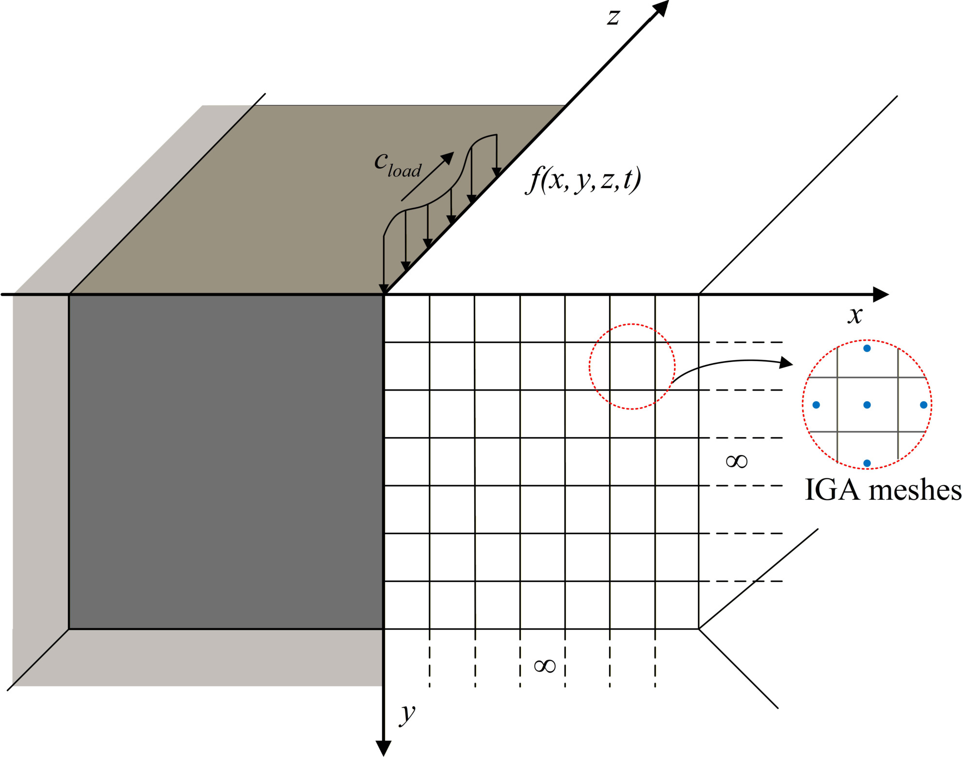
The equations of motion are written as \[\sigma_{ij,j}(\mathbf{x},t)+f_i(\mathbf{x},t)=\rho\,\ddot{u}_i(\mathbf{x},t), \qquad i,j\in\{1,2,3\}. \label{eq:G1}\tag{1}\] where \(\sigma_{ij}\) are the Cauchy stress components, \(f_i\) are the body-force components per unit volume (often neglected for moving surface or tunnel excitations), \(\rho\) is the mass density, \(\sigma_{ij,j}\) denotes \(\partial(\sigma_{ij})/\partial x_j\), and overdots denote partial derivatives with respect to time. Under the small-strain assumption, the infinitesimal strain tensor is defined by \[\varepsilon_{ij}(\mathbf{x},t)=\frac{1}{2}\left(u_{i,j}(\mathbf{x},t)+u_{j,i}(\mathbf{x},t)\right) \label{eq:G2}\tag{2}\] The linear constitutive law is expressed as \[\sigma_{ij}(\mathbf{x},t)=D_{ijkl}^\ast\,\varepsilon_{kl}(\mathbf{x},t) \label{eq:G3}\tag{3}\] where \(D_{ijkl}^\ast\) is the fourth-order complex constitutive tensor. In this study, material dissipation is represented through complex moduli (hysteretic damping). Specifically, the complex Young’s modulus is taken as \[E^\ast = E\left(1+2\mathrm{i}\zeta\right) \label{eq:E95complex}\tag{4}\] where \(\zeta\) is a dimensionless loss parameter and \(\mathrm{i}=\sqrt{-1}\). For an isotropic linear viscoelastic solid with hysteretic damping, the complex Lamé parameters are \[\lambda^\ast=\frac{\nu E^\ast}{(1+\nu)(1-2\nu)}, \qquad G^\ast=\frac{E^\ast}{2(1+\nu)} \label{eq:lame95complex}\tag{5}\] with \(\nu\) being Poisson’s ratio. The constitutive tensor then simplifies to \[D_{ijkl}^\ast=\lambda^\ast\,\delta_{ij}\delta_{kl}+G^\ast(\delta_{ik}\delta_{jl}+\delta_{il}\delta_{jk}) \label{eq:D95tensor95iso}\tag{6}\] where \(\delta_{ij}\) is the Kronecker delta. Substituting Eq. 2 and 6 into Eq. 1 yields the displacement-based Navier equation with complex moduli,
The boundary \(\Gamma=\partial\Omega\) is decomposed into \(\Gamma_u\) and \(\Gamma_t\) such that \(\Gamma=\Gamma_u\cup\Gamma_t\) and \(\Gamma_u\cap\Gamma_t=\varnothing\). The Dirichlet and Neumann boundary conditions are prescribed as \[u_i(\mathbf{x},t)=\bar{u}_i(\mathbf{x},t)\;\text{on}\;\Gamma_u, \qquad \sigma_{ij}(\mathbf{x},t)\,n_j(\mathbf{x})=\bar{t}_i(\mathbf{x},t)\;\text{on}\;\Gamma_t \label{eq:BCs}\tag{8}\] where \(n_j\) is the outward unit normal to \(\Gamma\), while \(\bar{u}_i\) and \(\bar{t}_i\) are the prescribed displacement and traction components, respectively. The initial conditions are \[u_i(\mathbf{x},0)=u_i^0(\mathbf{x}), \qquad \dot{u}_i(\mathbf{x},0)=v_i^0(\mathbf{x}) \qquad \text{in }\Omega \label{eq:ICs}\tag{9}\] where \(u_i^0\) and \(v_i^0\) denote the initial displacement and velocity fields. For a semi-infinite soil domain, the solution must additionally satisfy radiation or decay conditions as \(\|\mathbf{x}\|\to\infty\), which will be addressed in the unbounded-domain treatment detailed in Section 3.
2.2 2.5D reduction using Fourier transform and wavenumber-domain equations↩︎
The transformation from a full three-dimensional problem to a 2.5D formulation relies on the geometric invariance of the road/soil system along the traveling direction (\(z\)-axis). Since the material properties and cross-sectional geometry do not vary with \(z\), the linear viscoelastic dynamic response can be effectively decomposed using spectral methods.
We adopt a Fourier transform approach to decouple the spatial coordinate \(z\) and time \(t\). The displacement field \(u_i(\mathbf{x},t)\) is expressed as a superposition of harmonic waves. By assuming a time-harmonic behavior \(e^{\mathrm{i}\omega t}\) and a spatial wave propagation \(e^{-\mathrm{i}kz}\), the displacement ansatz is given by:
\[u_i(x,y,z,t)=\hat{u}_i(x,y;k,\omega)\,e^{-\mathrm{i}k z}\,e^{\mathrm{i}\omega t}, \qquad i\in\{1,2,3\}. \label{eq:2p5d95ansatz}\tag{10}\] Substitution of Eq. 10 into the governing equations derived in Section 2.1 reduces the three-dimensional problem to a family of two-dimensional boundary-value problems on the \((x,y)\) cross-section, parameterized by \((k,\omega)\). Specifically, the differential operators are mapped to the frequency-wavenumber domain as follows: \[\frac{\partial(\cdot)}{\partial z}\rightarrow -\mathrm{i}k(\cdot),\qquad \frac{\partial^2(\cdot)}{\partial z^2}\rightarrow -k^2(\cdot),\qquad \frac{\partial^2(\cdot)}{\partial t^2}\rightarrow -\omega^2(\cdot) \label{eq:2p5d95map}\tag{11}\] This transformation reduces the original 3D problem to a family of 2D boundary value problems defined over the cross-section \((x,y)\), which are computationally far more efficient to solve.
To retain consistency with this 2.5D framework, the moving loads must also be transformed into the frequency-wavenumber domain. The excitation caused by a convoy of vehicles moving at a constant speed \(c_{\mathrm{load}}\) is typically modeled as a separable function of space and time. Consider a general load component defined by \[F(x,y,z,t)=\psi(x,y)\,\phi(z-c_{\mathrm{load}}t)\sum_{j=1}^{n} T_{j}\,e^{\mathrm{i}\omega_{j} t} \label{eq:moving95load95general}\tag{12}\] where \(\psi(x,y)\) represents the transverse distribution of the load, \(\phi(z-c_{\mathrm{load}}t)\) describes the longitudinal footprint moving with the vehicle, and \(T_j\) denotes the amplitude of the \(j\)-th harmonic component with driving frequency \(\omega_j\).
For clarity, we derive the transformation for a single harmonic component \((T, \omega_0)\). The temporal Fourier transform is formally defined as: \[\tilde{F}(x,y,z,\omega)=\frac{1}{2\pi}\int_{-\infty}^{+\infty}F(x,y,z,t)\,e^{-\mathrm{i}\omega t}\,\mathrm{d}t \label{eq:FT95time95def}\tag{13}\] Substituting the load expression into Eq. 13 leads to the following. \[\tilde{F}(x,y,z,\omega)=\frac{T}{2\pi}\,\psi(x,y)\int_{-\infty}^{+\infty}\phi(z-c_{\mathrm{load}}t)\,e^{-\mathrm{i}(\omega-\omega_0)t}\,\mathrm{d}t \label{eq:FT95step1}\tag{14}\] To evaluate this integral, it is convenient to switch to a moving coordinate system. Introducing the change of variables \(\tau=z-c_{\mathrm{load}}t\), which implies \(t = (z-\tau)/c_{\mathrm{load}}, \qquad dt = -d\tau/c_{\mathrm{load}}\), allows us to decouple the oscillating term from the moving frame. Note that the integration limits are swapped during this substitution, canceling the negative sign from the differential. The expression thus becomes: \[\tilde{F}(x,y,z,\omega)=\frac{T}{c_{\mathrm{load}}}\,\psi(x,y)\,e^{-\mathrm{i}(\omega-\omega_0)z/c_{\mathrm{load}}} \left[ \frac{1}{2\pi}\int_{-\infty}^{+\infty}\phi(\tau)\,e^{\mathrm{i}(\omega-\omega_0)\tau/c_{\mathrm{load}}}\,\mathrm{d}\tau \right] \label{eq:FT95step2}\tag{15}\] The term within the brackets is recognized as the spatial Fourier transform of the longitudinal load function. By defining the equivalent longitudinal wavenumber \(k\) as \[k=\frac{\omega-\omega_0}{c_{\mathrm{load}}} \label{eq:k95def}\tag{16}\] and letting \(\tilde{\phi}(k)\) denote the spatial transform pair of \(\phi(\tau)\), \[\tilde{\phi}(k)=\frac{1}{2\pi}\int_{-\infty}^{+\infty}\phi(\tau)\,e^{-\mathrm{i}k\tau}\,\mathrm{d}\tau \label{eq:phi95FT95def}\tag{17}\] Eq. 15 simplifies to a compact form: \[\tilde{F}(x,y,z,\omega)=\frac{T}{c_{\mathrm{load}}}\,\psi(x,y)\,e^{-\mathrm{i}k z}\,\tilde{\phi}(-k) \label{eq:load95freq95domain95final}\tag{18}\] Eq. 16 and 18 reveal a fundamental characteristic of the moving load problem: the temporal frequency \(\omega\) and the longitudinal wavenumber \(k\) are not independent but are strictly coupled through the vehicle speed \(c\). This represents the Doppler shift effect inherent in moving source problems. Consequently, for a given source frequency \(\omega_0\) and speed \(c\), the response only needs to be computed at specific wavenumbers, significantly reducing the computational cost compared to a full 3D analysis. The total response for the multi-harmonic excitation in Eq. 12 is finally obtained by linear superposition of these individual components.
3 Isogeometric formulation for 2.5D moving-load problem↩︎
3.1 NURBS representation of the cross-section and displacement field↩︎
The isogeometric construction is performed on the \((x,y)\) cross-section \(\Omega_{2D}\); the longitudinal direction is represented by the wavenumber \(k\). The B-spline and NURBS definitions needed for the geometry and displacement spaces are summarized below to fix the notation used in the proposed infinite-element construction.
Let the open knot vector be \[\boldsymbol{\Xi}=\{\xi_1,\xi_2,\ldots,\xi_{n_b+p+1}\}\] where \(p\) is the polynomial degree and \(n_b\) is the number of one-dimensional basis functions. The Cox–de Boor recursion starts from \[B_{i,0}(\xi)= \begin{cases} 1, & \xi_i\le \xi<\xi_{i+1}\\ 0, & \text{otherwise} \end{cases} \label{eq:Bspline95p0}\tag{19}\] and for \(p\ge 1\), \[B_{i,p}(\xi)=\frac{\xi-\xi_i}{\xi_{i+p}-\xi_i}\,B_{i,p-1}(\xi) +\frac{\xi_{i+p+1}-\xi}{\xi_{i+p+1}-\xi_{i+1}}\,B_{i+1,p-1}(\xi) \label{eq:Bspline95recursion}\tag{20}\] Non-empty knot spans define the elements. A knot of multiplicity \(m\) gives \(C^{p-m}\) continuity; endpoint multiplicity \(p+1\) makes an open-knot B-spline basis interpolatory at both ends.
Given positive weights \(\{w_i\}_{i=1}^{n_b}\), the rational extension used to represent conic sections is \[N_{i,p}(\xi)=\frac{w_i B_{i,p}(\xi)}{\displaystyle\sum_{\hat{i}=1}^{n_b} w_{\hat{i}} B_{\hat{i},p}(\xi)} \label{eq:NURBS951D}\tag{21}\] A NURBS curve with control points \(\mathbf{P}_i\) is \[\mathbf{S}(\xi)=\sum_{i=1}^{n_b} N_{i,p}(\xi)\,\mathbf{P}_i \label{eq:NURBS95curve}\tag{22}\]
For the cross-section, tensor products in the parametric coordinates \((\xi,\eta)\) give the geometric mapping \[\mathbf{x}_{\perp}(\xi,\eta)=\sum_{A=1}^{n_{cp}} R_A(\xi,\eta)\,\mathbf{P}_A, \qquad \mathbf{x}_{\perp}=(x,y) \label{eq:geom95map}\tag{23}\] where \(R_A(\xi,\eta)\) are the bivariate NURBS basis functions, \(\mathbf{P}_A\) are the control points, and \(n_{cp}\) is their total number. The same \(R_A\) are used for the displacement approximation.
As in other wave discretizations, the element scale must resolve the smallest wavelength of interest to control dispersion and phase error. Spline order and continuity can be selected independently, while repeated knots reduce continuity at corners and material interfaces. These properties are valuable because the cross-sectional system is solved repeatedly over the required \((k,\omega)\) pairs.
Knot repetition changes continuity but does not make tensor-product refinement fully local. The present implementation therefore uses compatible multi-patch refinement to concentrate resolution near load paths, material interfaces, and curved internal boundaries while preserving a conforming NURBS trace on artificial-boundary segments.
The resulting displacement interpolation, geometric Jacobian, and physical derivatives are stated together with the 2.5D strain operator in the following subsection; standard NURBS differentiation follows [18].
3.2 Isogeometric discretization of the bounded cross-section in the wavenumber–frequency domain↩︎
For each prescribed pair \((k,\omega)\) arising from the 2.5D reduction in Section 2, the governing equations are posed on the bounded cross-section \(\Omega_{2D}\subset\mathbb{R}^2\) with physical coordinates \(\mathbf{x}_\perp\). An isogeometric discretization is adopted so that the cross-sectional geometry and the displacement amplitudes are represented by the same spline basis. This is particularly attractive in wave propagation analysis, where higher-order smooth bases can alleviate dispersion and pollution errors, and where knot multiplicity provides a direct mechanism to control continuity when geometric corners or material interfaces must be represented.
Let \((\xi,\eta)\in\widehat{\Omega}\) be the parametric coordinates of the NURBS surface defining the cross-section. For a given \((k,\omega)\), the displacement amplitudes are approximated as \[\hat{\mathbf{u}}(\mathbf{x}_\perp;k,\omega) = \sum_{A=1}^{n_{cp}} R_A(\xi,\eta)\,\mathbf{d}_A(k,\omega), \qquad \mathbf{d}_A= \begin{bmatrix} d_{xA} & d_{yA} & d_{zA} \end{bmatrix}^{T} \label{eq:IGA95u95interp}\tag{24}\] where \(\hat{\mathbf{u}}=[\hat{u}_x,\hat{u}_y,\hat{u}_z]^T\) and \(\mathbf{d}_A\) collects the three displacement degrees of freedom at control point \(A\). Introducing the global vector \(\mathbf{d}\) by stacking all \(\mathbf{d}_A\), the approximation takes the matrix form \[\hat{\mathbf{u}}=\mathbf{N}\mathbf{d}, \qquad \mathbf{N}= \begin{bmatrix} R_1\mathbf{I}_3 & R_2\mathbf{I}_3 & \cdots & R_{n_{cp}}\mathbf{I}_3 \end{bmatrix} \label{eq:IGA95N95matrix}\tag{25}\] with \(\mathbf{I}_3\) being the \(3\times 3\) identity matrix.
Spatial derivatives with respect to physical coordinates follow from parametric derivatives through the Jacobian of the geometric mapping. The Jacobian matrix is defined as \[\mathbf{J}(\xi,\eta)= \begin{bmatrix} \displaystyle \frac{\partial x}{\partial \xi} & \displaystyle \frac{\partial x}{\partial \eta} \\[6pt] \displaystyle \frac{\partial y}{\partial \xi} & \displaystyle \frac{\partial y}{\partial \eta} \end{bmatrix}, \qquad J=\det\mathbf{J} \label{eq:IGA95Jacobian}\tag{26}\] Accordingly, for each basis function \(R_A\), the physical derivatives are obtained as \[\begin{bmatrix} \displaystyle \frac{\partial R_A}{\partial x} \\[6pt] \displaystyle \frac{\partial R_A}{\partial y} \end{bmatrix} = \mathbf{J}^{-T} \begin{bmatrix} \displaystyle \frac{\partial R_A}{\partial \xi} \\[6pt] \displaystyle \frac{\partial R_A}{\partial \eta} \end{bmatrix} \label{eq:IGA95grad95transform}\tag{27}\]
With the harmonic dependence \(e^{-\mathrm{i}k z}e^{\mathrm{i}\omega t}\), differentiation with respect to \(z\) is replaced by multiplication with \(-\mathrm{i}k\). Using engineering strains, the strain vector is defined as: \[\boldsymbol{\varepsilon}= \begin{bmatrix} \varepsilon_{xx} & \varepsilon_{yy} & \varepsilon_{zz} & \gamma_{xy} & \gamma_{yz} & \gamma_{xz} \end{bmatrix}^{T} \label{eq:strain95vector95def}\tag{28}\] with components \[\varepsilon_{xx}=\frac{\partial \hat{u}_x}{\partial x},\quad \varepsilon_{yy}=\frac{\partial \hat{u}_y}{\partial y},\quad \varepsilon_{zz}=-\mathrm{i}k\,\hat{u}_z,\quad \gamma_{xy}=\frac{\partial \hat{u}_x}{\partial y}+\frac{\partial \hat{u}_y}{\partial x},\quad \gamma_{yz}=\frac{\partial \hat{u}_z}{\partial y}-\mathrm{i}k\,\hat{u}_y,\quad \gamma_{xz}=\frac{\partial \hat{u}_z}{\partial x}-\mathrm{i}k\,\hat{u}_x \label{eq:2p5d95strains}\tag{29}\] Substituting Eq. 24 into Eq. 29 yields \[\boldsymbol{\varepsilon}=\mathbf{B}(k)\mathbf{d}, \qquad \mathbf{B}(k)= \begin{bmatrix} \mathbf{B}_1(k) & \mathbf{B}_2(k) & \cdots & \mathbf{B}_{n_{cp}}(k) \end{bmatrix} \label{eq:B95global}\tag{30}\] where the \(6\times 3\) block associated with control point \(A\) is \[\mathbf{B}_A(k)= \begin{bmatrix} R_{A,x} & 0 & 0 \\ 0 & R_{A,y} & 0 \\ 0 & 0 & -\mathrm{i}k\,R_A \\ R_{A,y} & R_{A,x} & 0 \\ 0 & -\mathrm{i}k\,R_A & R_{A,y} \\ -\mathrm{i}k\,R_A & 0 & R_{A,x} \end{bmatrix} \label{eq:B95block}\tag{31}\] with \(R_{A,x}=\partial R_A/\partial x\) and \(R_{A,y}=\partial R_A/\partial y\) computed from Eq. 27 .
In the wavenumber–frequency domain, material dissipation is represented through complex-valued moduli. The stress–strain relation is written in Voigt form as \[\boldsymbol{\sigma}= \mathbf{D}^\ast \boldsymbol{\varepsilon}, \qquad \boldsymbol{\sigma}= \begin{bmatrix} \sigma_{xx} & \sigma_{yy} & \sigma_{zz} & \tau_{xy} & \tau_{yz} & \tau_{xz} \end{bmatrix}^{T} \label{eq:constitutive95voigt}\tag{32}\] with \[\mathbf{D}^\ast= \begin{bmatrix} \lambda^\ast+2G^\ast & \lambda^\ast & \lambda^\ast & 0 & 0 & 0 \\ \lambda^\ast & \lambda^\ast+2G^\ast & \lambda^\ast & 0 & 0 & 0 \\ \lambda^\ast & \lambda^\ast & \lambda^\ast+2G^\ast & 0 & 0 & 0 \\ 0 & 0 & 0 & G^\ast & 0 & 0 \\ 0 & 0 & 0 & 0 & G^\ast & 0 \\ 0 & 0 & 0 & 0 & 0 & G^\ast \end{bmatrix} \label{eq:Dstar95matrix}\tag{33}\]
A Galerkin discretization in the wavenumber–frequency domain yields, for each \((k,\omega)\), \[\bigl[\mathbf{K}(k)-\omega^2\mathbf{M}\bigr]\mathbf{d}(k,\omega)=\mathbf{f}(k,\omega) \label{eq:discrete95system95kw}\tag{34}\] where \(\mathbf{K}(k)\) is complex-valued through \(\mathbf{D}^\ast\) and \(\mathbf{M}\) is real-valued. The global matrices are assembled from element contributions. Denoting the parametric element domain by \(\widehat{\Omega}_e\), the element stiffness and mass matrices are computed as \[\mathbf{K}_e(k)=\int_{\widehat{\Omega}_e}\mathbf{B}_e^{H}(k)\,\mathbf{D}^\ast\,\mathbf{B}_e(k)\,J\,\mathrm{d}\xi\,\mathrm{d}\eta, \qquad \mathbf{M}_e=\int_{\widehat{\Omega}_e}\rho\,\mathbf{N}_e^{T}\mathbf{N}_e\,J\,\mathrm{d}\xi\,\mathrm{d}\eta \label{eq:Ke95Me95param}\tag{35}\] where \((\cdot)^{H}\) denotes the conjugate transpose, and \(\rho\) is the mass density. Numerical integration is performed by Gaussian quadrature of sufficiently high order to capture the rational character of the NURBS basis functions and the required accuracy in wave propagation computations.
For the corresponding lossless reference material with real-valued \(\mathbf{D}\), the \(k\)-dependence of \(\mathbf{B}(k)\) implies a quadratic decomposition of the stiffness matrix, \[\mathbf{K}(k)=\mathbf{K}_0+\mathrm{i}k\,\mathbf{K}_1+k^2\mathbf{K}_2 \label{eq:K95decomp}\tag{36}\] where \(\mathbf{K}_0\), \(\mathbf{K}_1\), and \(\mathbf{K}_2\) are \(k\)-independent matrices assembled from the corresponding \(k^0\), \(k^1\), and \(k^2\) contributions in \(\mathbf{B}(k)\). The decomposition Eq. 36 remains valid when complex moduli are used, while Hermitian symmetry is generally lost.
The load vector \(\mathbf{f}(k,\omega)\) corresponds to the consistent forces induced by the transformed traction boundary conditions on \(\Gamma_t\), \[\mathbf{f}(k,\omega)=\int_{\Gamma_t}\mathbf{N}^{H}\hat{\mathbf{t}}(\mathbf{x}_\perp;k,\omega)\,\mathrm{d}\Gamma \label{eq:load95vector95kw}\tag{37}\] where \(\hat{\mathbf{t}}(\mathbf{x}_\perp;k,\omega)\) is the traction amplitude in the wavenumber–frequency domain.
3.3 2.5D NURBS-trace infinite elements for enforcing radiation conditions↩︎
For each prescribed pair \((k,\omega)\) arising from the 2.5D reduction in Section 2, the cross-sectional problem is posed on \(\Omega_{2D}\subset\mathbb{R}^2\) with physical coordinates \(\mathbf{x}_\perp=(x,y)\). The bounded near field is denoted by \(\Omega_n\) and is coupled to the semi-infinite exterior \(\Omega_f\) through the artificial boundary \(\Gamma_b\). Thus, \[\Omega_{2D}=\Omega_n\cup\Omega_f, \qquad \Gamma_b=\partial\Omega_n\cap\partial\Omega_f .\] In the discrete formulation, the artificial boundary is represented by trace segments \(\Gamma_b^q\) satisfying \(\Gamma_b=\cup_q\Gamma_b^q\). The near field is discretized by the NURBS-based isogeometric formulation described in Subsection 3.2, while the exterior contribution associated with each trace segment is represented by infinite elements. Their role is to approximate the exterior response by combining the boundary trace with radial functions that satisfy the required outgoing or decay behavior.
The following construction separates the invariant trace-space principle from the selectable radial approximation.
An outward coordinate \(\xi_\infty\in[0,\infty)\) is introduced on each segment of the artificial boundary. The unbounded direction is represented by a radial function \[P_q=P_q(\xi_\infty;k,\omega,\boldsymbol{\theta}_q), \qquad P_q(0;k,\omega,\boldsymbol{\theta}_q)=1, \label{eq:IE95propagation95IGA}\tag{38}\] where \(q\) identifies a boundary segment or an admissible radial model and \(\boldsymbol{\theta}_q\) denotes its radial parameters. Equation 38 deliberately does not prescribe a particular exponential, decay coefficient, or spatial partition. These choices determine the radiation accuracy of a realization of the method, but they do not alter its trace-space construction.
The admissible radial family is defined by three requirements. First, the normalization \(P_q(0)=1\) preserves the finite-dimensional trace at the near–far-field interface. Second, \(P_q\) must represent an outgoing or evanescent contribution and contain no component that grows toward infinity. Third, \(P_q\) and its radial derivative must make the far-field weak forms finite. In a mapped radial coordinate, the last requirement can be expressed abstractly as \[\int_0^\infty \left( |P_q(\xi_\infty)|^2 + |\partial_{\xi_\infty}P_q(\xi_\infty)|^2 \right) w_q(\xi_\infty)\,\mathrm{d}\xi_\infty <\infty, \label{eq:radial95admissibility}\tag{39}\] where \(w_q\) accounts for the algebraic growth introduced by the far-field mapping. For an undamped propagating contribution, the outgoing solution is understood through the limiting-absorption principle. Consequently, a vanishing explicit decay coefficient is admissible only when the complete radial factor remains outgoing and the associated weak forms are well defined.
The 2.5D reduction fixes the longitudinal wavenumber of a moving harmonic load as \[k=\frac{\omega-\omega_0}{c_{\mathrm{load}}}. \label{eq:k95moving95load95in95IE}\tag{40}\] For an isotropic exterior medium, the bulk or surface-wave dispersion relations provide candidate transverse wavenumbers through \[\kappa_i^2=k_i^2-k^2, \qquad k_i=\frac{\omega}{c_i}. \label{eq:kappa95def95infinite}\tag{41}\] The physically relevant branch is selected by the outgoing radiation condition, equivalently by continuation from a weakly dissipative medium. This principle covers propagating, evanescent, and damped components without tying the formulation to a code-dependent algebraic sign convention. Candidate wave-informed functions may be used to construct \(P_q\), while their adequacy for a finite truncation boundary is evaluated by the controlled numerical assessment in Section 4.1.
The numerical study uses an all-S realization, in which the S-wave-informed radial family is assigned to every artificial-boundary segment. Its explicit radial factor is \[P_q(\xi_\infty) = \exp\!\left[-\left(\alpha_{S,q}-\mathrm{i}\kappa_S\right)\xi_\infty\right], \qquad \kappa_S = \left[\left(\frac{\omega}{c_{S,\infty}}\right)^2-k^2\right]_{\mathrm{out}}^{1/2}, \label{eq:allS95radial95factor}\tag{42}\] where the subscript “out” denotes the outgoing branch. Its reference decay is \[\alpha_{S,q}^{\mathrm{ref}} = \frac{1}{2L_q} \left( 1+\frac{k^2}{k^2+\kappa_S^2} \right). \label{eq:alphaS95reference}\tag{43}\] Here \(L_q\) is the characteristic outward distance assigned to segment \(q\) by the radial map. For the rectangular domains used in the verification and engineering examples, \(L_q=R\) on the lateral boundary and \(L_q=H\) on the lower boundary. Thus, \(L_q\) is a declared geometric input rather than a fitted material parameter; a non-rectangular radial map must analogously store its segment-wise characteristic distance. In damped calculations, \(c_{S,\infty}=\sqrt{G_\infty/\rho_\infty}\) is the reference speed computed from the storage modulus \(G_\infty=E_\infty/[2(1+\nu_\infty)]\). Material attenuation remains in the complex tensor \(\mathbf{D}^{\ast}\) of Eq. 6 ; a complex wave speed is not substituted into Eqs. 41 and 43 .

The far-field geometry preserves the NURBS representation of the truncation boundary and extends it in the outward direction through a radial mapping. Let \(s\in[0,1]\) be the parametric coordinate along the boundary segment \(\Gamma_b^q\), with NURBS basis functions \(\{R_{A,q}^{b}(s)\}_{A=1}^{n_{b,q}}\) and boundary control points \(\{\mathbf{P}_{A,q}^{b}\}_{A=1}^{n_{b,q}}\). The segment geometry is \[\mathbf{x}_{b,q}(s) = \sum_{A=1}^{n_{b,q}}R_{A,q}^{b}(s)\,\mathbf{P}_{A,q}^{b}, \qquad \mathbf{x}_{b,q}=(x_{b,q},y_{b,q}). \label{eq:boundary95curve95nurbs}\tag{44}\]
The discrete compatibility on each segment can now be stated precisely. Let \(\mathcal{V}_h^n\) be the vector-valued near-field IGA trial space, let \(\gamma_{b,q}\) denote its trace on \(\Gamma_b^q\), and let \(\{\mathbf{e}_\ell\}_{\ell=1}^{3}\) be the Cartesian basis. The near-field trace space associated with segment \(q\) is \[\mathcal{T}_{h,q} := \gamma_{b,q}\mathcal{V}_h^n = \operatorname{span} \left\{ R_{A,q}^b(s)\mathbf{e}_\ell: A=1,\ldots,n_{b,q},\;\ell=1,2,3 \right\}. \label{eq:nurbs95trace95space}\tag{45}\] For a far-field segment \(q\), the proposed trial space is the tensor product \[\mathcal{V}_{h,q}^f = \operatorname{span} \left\{ R_{A,q}^b(s)P_q(\xi_\infty)\mathbf{e}_\ell: A=1,\ldots,n_{b,q},\;\ell=1,2,3 \right\}. \label{eq:far95field95trial95space}\tag{46}\] Because \(P_q(0)=1\), its boundary trace satisfies \[\left.\mathcal{V}_{h,q}^f\right|_{\xi_\infty=0} = \mathcal{T}_{h,q} = \gamma_{b,q}\mathcal{V}_h^n. \label{eq:trace95space95conformity}\tag{47}\] Equation 47 is the precise meaning of NURBS-trace consistency in this work: the two discrete traces coincide on each artificial-boundary segment and share their coefficients. The global far-field space \(\mathcal{V}_h^f\) is assembled from the segment spaces \(\mathcal{V}_{h,q}^f\), with common trace coefficients identified at shared boundary control points. This construction does not assert that the unbounded radial direction is itself represented by NURBS; that direction is represented by the analytical function \(P_q\).
The geometry of an infinite segment is described by a regular mapping \[\mathbf{x}_\perp = \mathcal{F}_q(s,\xi_\infty), \qquad \mathcal{F}_q(s,0)=\mathbf{x}_{b,q}(s), \qquad \|\mathcal{F}_q(s,\xi_\infty)\|\rightarrow\infty \quad\text{as }\xi_\infty\rightarrow\infty. \label{eq:IE95geom95tensor}\tag{48}\] Only the interface condition and regularity of \(\mathcal{F}_q\) are essential to the trace coupling. Pole-based, normal-extrusion, or other admissible radial mappings may therefore be used without changing the discrete interface space, provided that the mapping remains one-to-one and its Jacobian is nonsingular.
In the numerical implementation, the far-field matrices are assembled from the infinite-element contributions associated with the artificial-boundary segments. The segment mapping \(\mathcal{F}_q\) supplies the geometric Jacobian in the boundary-coordinate integrals, while the radial dependence is carried by \(P_q\) and its derivative.
The coefficient realization of Eqs. 46 –47 is obtained as follows. Let \[\mathbf{d}_{A,q}(k,\omega) = [d_{xA,q},d_{yA,q},d_{zA,q}]^T\] be the displacement-amplitude vector at segment boundary control point \(A\); this local coefficient is identified with the corresponding global trace unknown. For a far-field segment \(q\), the displacement amplitude is approximated as \[\hat{\mathbf{u}}^{\,f}(s,\xi_\infty;k,\omega) = \sum_{A=1}^{n_{b,q}} R_{A,q}^{b}(s)\,P_q(\xi_\infty)\,\mathbf{d}_{A,q}(k,\omega). \label{eq:IE95u95tensor}\tag{49}\] At \(\xi_\infty=0\), Eq. 49 reduces to the near-field boundary interpolation. Displacement continuity is therefore imposed by coefficient identification, without projection, mortar variables, or an additional interface transfer operation.
Derivatives with respect to \((x,y)\) follow from the Jacobian of the mapping in Eq. 48 . Define \[\mathbf{J}_f(s,\xi_\infty) = \frac{\partial\mathbf{x}_\perp}{\partial(s,\xi_\infty)}, \qquad J_f=\det\mathbf{J}_f . \label{eq:IE95Jacobian}\tag{50}\] Define the tensor-product basis \(\Phi_{A,q}(s,\xi_\infty)=R_{A,q}^b(s)P_q(\xi_\infty)\). Its cross-sectional derivatives follow from the chain rule through \(\mathbf{J}_f^{-T}\), while the longitudinal derivative is represented by the same wavenumber operator used in the near field. Consequently, the far-field strain retains all six components of the 2.5D linear viscoelastic vector wave problem and can be written as \[\boldsymbol{\varepsilon}^{\,f} = \mathbf{B}_f(k)\mathbf{d}_b , \label{eq:IE95B95IGA}\tag{51}\] where \(\mathbf{d}_b\) stacks the boundary control-point degrees of freedom. The operator \(\mathbf{B}_f(k)\) is obtained from the standard 2.5D strain operator applied to \(\Phi_{A,q}\); its detailed entries depend only on the declared Fourier convention and coordinate orientation. The radial model therefore changes the exterior approximation through \(P_q\) and \(\partial_{\xi_\infty}P_q\), without reducing the vector problem to a scalar or plane-strain model.
For each \((k,\omega)\), the near- and far-field approximations form the conforming coupled space, where \(\gamma_b\) denotes the assembled trace operator on \(\Gamma_b\): \[\mathcal{V}_h = \left\{ (\mathbf{v}_h^n,\mathbf{v}_h^f) \in\mathcal{V}_h^n\times\mathcal{V}_h^f: \gamma_b\mathbf{v}_h^n = \left.\mathbf{v}_h^f\right|_{\xi_\infty=0} \right\}. \label{eq:coupled95trace95space}\tag{52}\] The discrete problem is obtained from the same frequency-domain weak form in both subdomains: find \(\mathbf{u}_h\in\mathcal{V}_h\) such that \[a_n(\mathbf{v}_h,\mathbf{u}_h) +a_f(\mathbf{v}_h,\mathbf{u}_h) -\omega^2 \left[ m_n(\mathbf{v}_h,\mathbf{u}_h) +m_f(\mathbf{v}_h,\mathbf{u}_h) \right] = \ell(\mathbf{v}_h) \label{eq:coupled95weak95form}\tag{53}\] for all admissible test functions \(\mathbf{v}_h\). The far-field forms are \[\begin{align} a_f(\mathbf{v}_h,\mathbf{u}_h) &= \int_{\Omega_f} \boldsymbol{\varepsilon}(\mathbf{v}_h)^{H} \mathbf{D}^{\ast} \boldsymbol{\varepsilon}(\mathbf{u}_h) \,\mathrm{d}\Omega,\\ m_f(\mathbf{v}_h,\mathbf{u}_h) &= \int_{\Omega_f} \mathbf{v}_h^{H}\rho\mathbf{u}_h \,\mathrm{d}\Omega, \end{align} \label{eq:far95field95forms}\tag{54}\] with the corresponding near-field forms defined in Subsection 3.2. The superscript \(H\) denotes the conjugate transpose under the adopted complex test-space convention.
Because the interface coefficients are shared, assembly of Eq. 53 gives the global system \[\left[ \mathbf{K}_n(k)+\mathbf{K}_f(k) -\omega^2\left(\mathbf{M}_n+\mathbf{M}_f\right) \right]\mathbf{d} = \mathbf{f}(k,\omega). \label{eq:global95coupled95IGA95IE}\tag{55}\] No projection, penalty, mortar variable, or separately interpolated interface traction is required. For Eq. 42 , let \(\gamma_q=\alpha_{S,q}-\mathrm{i}\kappa_S\). The radial moments required by both far-field matrices are evaluated analytically; in particular, \[I_{0,q} =\int_0^\infty P_q\overline{P_q}\,\mathrm{d}\xi_\infty =\frac{1}{\gamma_q+\overline{\gamma_q}}, \qquad \Re(\gamma_q)>0, \label{eq:radial95moment95exact}\tag{56}\] and derivative moments follow by multiplication with \(-\gamma_q\) and \(-\overline{\gamma_q}\). In the optional calibrated comparison, a zero multiplier only removes the additional reference decay; the corresponding basis is retained only when the outgoing or evanescent part still gives \(\Re(\gamma_q)>0\). An undamped propagating factor with both zero explicit decay and \(\Re(\gamma_q)=0\) is rejected because Eq. 56 is then divergent. Hence no finite radial cutoff or radial quadrature is introduced in the production matrices. The remaining boundary-coordinate integrals use \(n_g=\max(3,p_b+1)\) Gauss–Legendre points on every nonzero NURBS knot span, where \(p_b\) is the degree of the boundary trace. Section 4.1 verifies the analytical radial moments independently by direct adaptive complex integration on the native interval \([0,\infty)\), without a user-defined finite cutoff or variable transformation, and reports the tolerances and matrix norm used in that audit. The boundary quadrature is separately checked by repeating the cubic-trace response with three, four, and five points per knot span.
This construction separates the invariant contribution of the proposed NBIEM from the selectable exterior model. The invariant part is the tensor product of an admissible radial function with the NURBS trace of the bounded discretization, together with coefficient-level continuity in Eq. 47 . The radial family, its parameters, and the truncation distance influence approximation quality and may be revised without changing this coupling principle. Section 4.1 therefore assesses these choices through response sensitivity and boundary enlargement instead of treating a particular empirical parameter formula as part of the mathematical definition.
4 Numerical verification and methodological assessment↩︎
This section evaluates the proposed NBIEM through a series of numerical studies with increasing complexity. The studies are designed to assess three main aspects of the formulation: (i) the interior-field accuracy of the NURBS-based discretization for displacement and stress responses; (ii) the radiation performance of the NURBS-based infinite elements, including boundary-sensitivity checks, low-frequency radial sensitivity, and comparison with existing boundary-treatment strategies; and (iii) the applicability of the method to heterogeneous and engineering-oriented geotechnical configurations involving material interfaces, geometric transitions, and embedded structures.
The first group of tests uses closed-form half-space solutions to verify displacement and stress frequency-response functions under different moving-load speed regimes. The second group focuses on the artificial-boundary treatment at low frequencies, where boundary effects are more pronounced, and uses the same setting to assess the default radial workflow, examine an optional calibrated comparison, and compare NBIEM with FEM/IEM and IGA/SBIGA in terms of accuracy, phase response, and computational cost. The remaining examples consider layered ground, ballastless-track sections, and buried-structure configurations, illustrating the use of the formulation in engineering-oriented geotechnical models with multi-material domains and locally refined multi-patch discretizations. Unless otherwise stated, the baseline configuration is a homogeneous linear viscoelastic half-space, optionally containing a buried structure, subjected to a time-harmonic load traveling at a constant speed \(c_{\mathrm{load}}\) along the longitudinal direction, with load position \(z(t)=c_{\mathrm{load}}\,t\). The gravitational acceleration is fixed at \(g=9.81~\mathrm{m/s^2}\). The numerical settings are chosen to isolate wave-propagation, boundary-treatment, discretization, and load-speed effects.
4.1 Verification examples↩︎
4.1.1 Interior-field verification at relatively high frequency↩︎
The first verification study considers benchmark half-space problems with closed-form solutions to assess the interior-field accuracy of the proposed formulation in a controlled setting. A relatively high-frequency case is selected because it provides a stringent test of the spatial discretization, while the influence of the truncation boundary remains limited. Accordingly, the present results are interpreted primarily as a verification of the interior displacement and stress responses, whereas the boundary treatment and the selection of the infinite-element parameter \(\alpha\) are examined separately in the following subsection under low-frequency conditions. Owing to symmetry with respect to the vertical plane containing the load trajectory, only one half of the domain is discretized using an isogeometric analysis (IGA) mesh, and the far-field radiation condition is imposed through isogeometric infinite elements. For the half-space considered in this verification study, the compressional, shear, and Rayleigh wave speeds are \(c_P=173.2~\mathrm{m/s}\), \(c_S=100~\mathrm{m/s}\), and \(c_R=92.1~\mathrm{m/s}\), respectively. To control discretization-induced dispersion and maintain phase accuracy at the excitation frequency, the minimum near-field range \(R\) and the maximum element size \(L\) are selected using a fixed wavelength-based resolution criterion. The selected near-field range and element size satisfy \[\label{eq:mesh95rule} L \le \frac{\lambda_s'}{6}, \qquad R \ge \frac{\lambda_s'}{2}, \qquad \lambda_s'=\frac{2\pi}{k_s'} ,\tag{57}\] where \(\lambda_s'\) is the effective shear wavelength and \(k_s'\) is the magnitude of the corresponding transverse shear wavenumber associated with the moving-load problem, \[k_s'=\left|\left[\left(\frac{\omega}{c_S}\right)^2-\left(\frac{\omega-\omega_0}{c_{\mathrm{load}}}\right)^2\right]^{1/2}\right|.\] For the present benchmark, the mesh is selected according to the most restrictive requirement among the tested cases and is then kept unchanged for the different load speeds.
All results are reported in a normalized form. In the frequency domain, the normalized displacements are defined by \[\label{eq:norm95freq95disp} \tilde{U}=\frac{2\pi G}{c_{\mathrm{load}}}\,\tilde{u}(\mathrm{i}\omega), \qquad \tilde{V}=\frac{2\pi G}{c_{\mathrm{load}}}\,\tilde{v}(\mathrm{i}\omega), \qquad \tilde{W}=\frac{2\pi G}{c_{\mathrm{load}}}\,\tilde{w}(\mathrm{i}\omega),\tag{58}\] where \(G\) is the shear modulus and \(\omega\) is the angular frequency.
To verify the interior-field accuracy of the proposed formulation, a homogeneous half-space without a buried structure is first considered, with the mass density taken as \(\rho=2000~\mathrm{kg/m^3}\). Three representative speed regimes are examined: a sub-Rayleigh case (\(c_{\mathrm{load}}=90~\mathrm{m/s}\)), a super-shear but sub-compressional case (\(c_{\mathrm{load}}=120~\mathrm{m/s}\)), and a super-compressional case (\(c_{\mathrm{load}}=200~\mathrm{m/s}\)). The material damping ratio of the half-space is set to \(\zeta=0.05\).
The analytical displacement frequency-response functions follow [8]: \[\label{eq:yang95frf95disp} \tilde{u}_j(\omega) =\frac{1}{2\pi\mu}\int_{-\infty}^{\infty} \frac{-\mathrm{i}k_x}{2Q} \left[ \left(k_j^2+k_x^2-\frac{1}{2}k_s^2\right)\exp(-m_1 y) - m_1 m_2 \exp(-m_2 y) \right] \exp(\mathrm{i}k_x x)\,\mathrm{d}k_x ,\tag{59}\] \[\label{eq:yang95frf95disp95v} \tilde{v}_j(\omega) =\frac{1}{2\pi\mu}\int_{-\infty}^{\infty} \frac{-m_1}{2Q} \left[ \left(k_j^2+k_x^2-\frac{1}{2}k_s^2\right)\exp(-m_1 y) -\left(k_j^2+k_x^2\right)\exp(-m_2 y) \right] \exp(\mathrm{i}k_x x)\,\mathrm{d}k_x ,\tag{60}\] \[\label{eq:yang95frf95disp95w} \tilde{w}_j(\omega) =\frac{1}{2\pi\mu}\int_{-\infty}^{\infty} \frac{\mathrm{i}k_j}{2Q} \left[ \left(k_j^2+k_x^2-\frac{1}{2}k_s^2\right)\exp(-m_1 y) - m_1 m_2 \exp(-m_2 y) \right] \exp(\mathrm{i}k_x x)\,\mathrm{d}k_x .\tag{61}\] Here \(\mu\) denotes the shear modulus, \(k_x\) is the Fourier integration variable, and \(k_j=\omega/c_{\mathrm{load}}\) is the longitudinal wavenumber associated with the moving load. The compressional and shear wavenumbers are \(k_p=\omega/c_P\) and \(k_s=\omega/c_S\). The auxiliary quantities are \[\label{eq:Q95m195m295def} Q=\left(k_j^2+k_x^2-\frac{1}{2}k_s^2\right)^2 - m_1 m_2\left(k_j^2+k_x^2\right),\qquad m_1=\left(k_j^2+k_x^2-k_p^2\right)^{1/2},\qquad m_2=\left(k_j^2+k_x^2-k_s^2\right)^{1/2}.\tag{62}\]
The near-field truncation radius and the vertical extent of the computational domain are set to \(R=10~\mathrm{m}\) and \(H=10~\mathrm{m}\), respectively. In this frequency-domain verification, the excitation frequency is fixed at \(f=\omega/(2\pi)=32~\mathrm{Hz}\). The complex vertical and longitudinal displacement components, denoted by \(\tilde{V}_y\) and \(\tilde{W}_y\), are compared with the analytical solutions in Eqs. 60 and 61 . The results are shown in Figs. 3–5 for three representative load-speed regimes: \(c_{\mathrm{load}}=90~\mathrm{m/s}\) (sub-Rayleigh), \(120~\mathrm{m/s}\) (\(c_S<c_{\mathrm{load}}<c_P\)), and \(200~\mathrm{m/s}\) (super-compressional).
For each speed, panels (a) and (c) show the profiles along the \(x\)-direction at \(y=1~\mathrm{m}\), whereas panels (b) and (d) show the depth-wise variation along \(y\) at \(x=0~\mathrm{m}\). As \(c_{\mathrm{load}}\) increases, the responses along the \(x\)-direction evolve from a predominantly non-oscillatory decay at \(90~\mathrm{m/s}\) to clearly oscillatory patterns at \(120~\mathrm{m/s}\) and \(200~\mathrm{m/s}\), consistent with the increasing spatial wavenumber content of the steady-state field. In all three regimes, both IGA and FEM reproduce the analytical real and imaginary parts with good agreement, indicating that the displacement responses are accurately captured within the interior domain for the present test cases.

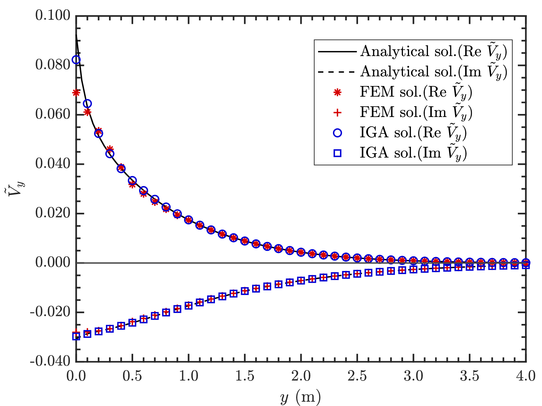
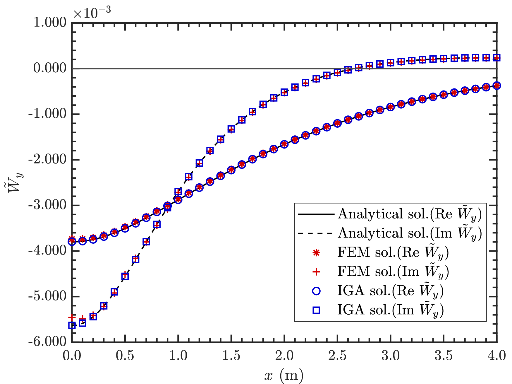

Figure 3: Frequency-domain displacement components \(\tilde{V}_y\) (vertical) and \(\tilde{W}_y\) (longitudinal) for \(f=32~\mathrm{Hz}\), \(f_0=0~\mathrm{Hz}\), \(c_{\mathrm{load}}=90~\mathrm{m/s}\) (sub-Rayleigh, \(c_{\mathrm{load}}<c_R\)), and \(\zeta=0.05\). Panels (a) and (c): \(x\)-profiles at \(y=1~\mathrm{m}\). Panels (b) and (d): depth-wise profiles along \(y\) extracted at \(x=0~\mathrm{m}\) (same extraction location for all methods). IGA and FEM are compared under matched spatial resolution (same maximum element size \(L\)) against the analytical solutions in Eqs. 60 and 61 ..
Under matched spatial resolution, i.e., with the same maximum element size \(L\), the depth-wise profiles show slightly smaller near-surface discrepancies for IGA in both \(\tilde{V}_y\) and \(\tilde{W}_y\), whereas FEM exhibits somewhat larger deviations in the same region. This trend is consistent with the higher-order continuity of spline bases in IGA, which improves the representation of near-surface gradients and reduces dispersion error in fixed-frequency wave propagation.
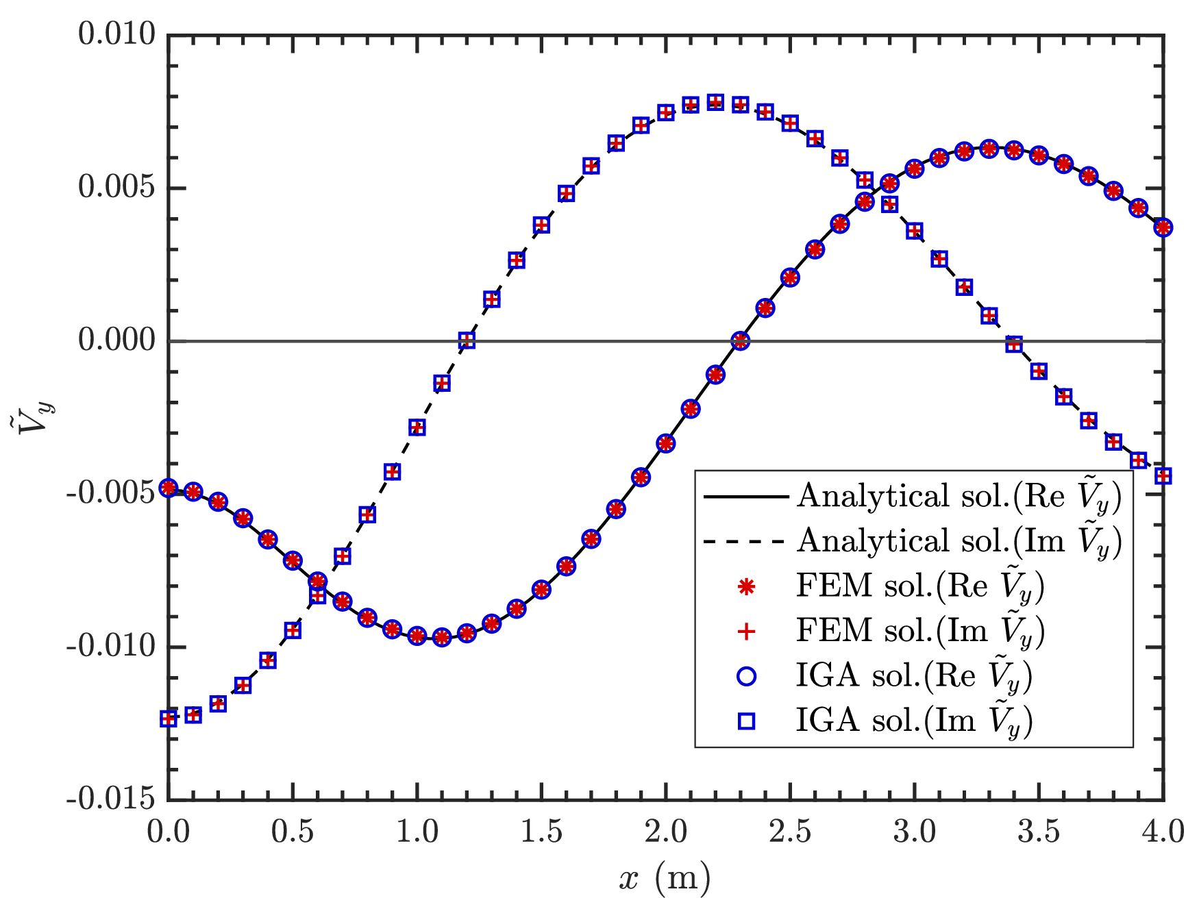


Figure 4: Frequency-domain displacements \(\tilde{V}_y\) and \(\tilde{W}_y\) for \(f=32~\mathrm{Hz}\), \(f_0=0~\mathrm{Hz}\), \(c_{\mathrm{load}}=120~\mathrm{m/s}~(c_S<c_{\mathrm{load}}<c_P)\), and \(\zeta=0.05\). (a) and (c) along the \(x\)-axis at \(y=1~\mathrm{m}\). (b) and (d) along the \(y\)-axis..


Figure 5: Frequency-domain displacements \(\tilde{V}_y\) and \(\tilde{W}_y\) for \(f=32~\mathrm{Hz}\), \(f_0=0~\mathrm{Hz}\), \(c_{\mathrm{load}}=200~\mathrm{m/s}~(c_{\mathrm{load}}>c_P)\), and \(\zeta=0.05\). (a) and (c) along the \(x\)-axis at \(y=1~\mathrm{m}\). (b) and (d) along the \(y\)-axis..
To assess the effect of a nonzero self-oscillation term, the displacement verification is repeated with \(f_0=10~\mathrm{Hz}\) while keeping \(f=32~\mathrm{Hz}\) fixed. The corresponding results are shown in Fig. 6. As shown in Fig. 6, both IGA and FEM remain in good agreement with the analytical solution for the real and imaginary parts of \(\tilde{V}_y\) and \(\tilde{W}_y\), both along the \(x\)-direction at \(y=1~\mathrm{m}\) and in the depth-wise profiles. Compared with the case \(f_0=0\), the \(x\)-profiles become more oscillatory, indicating increased high-wavenumber content and a higher demand for spatial resolution. Under the same mesh resolution, IGA continues to match the analytical curves more closely near the free surface in panels (b) and (d), while FEM shows slightly larger deviations. This observation aligns with the improved smoothness and dispersion properties of the IGA basis functions in single-frequency wave computations.


Figure 6: Frequency-domain displacement components \(\tilde{V}_y\) and \(\tilde{W}_y\) for \(f=32~\mathrm{Hz}\), \(f_0=10~\mathrm{Hz}\), \(c_{\mathrm{load}}=90~\mathrm{m/s}\), and \(\zeta=0.05\). Panels (a) and (c): \(x\)-profiles at \(y=1~\mathrm{m}\). Panels (b) and (d): depth-wise profiles along \(y\) extracted at \(x=0~\mathrm{m}\). The case \(f_0\neq 0\) yields a more oscillatory spatial response along \(x\), increasing the resolution demand..
In addition to the displacement FRFs, stress FRFs are computed and validated. The analytical expressions for the stress components are given in Eqs. 63 –68 .
\[\begin{align} \tilde{\sigma}_{xx,j}(\omega) &= \frac{1}{2\pi\mu}\int_{-\infty}^{\infty}\frac{1}{Q} \left[ \begin{aligned} &\Big(\frac{\nu}{1-2\nu}k_p^2+k_x^2\Big)\Big(k_j^2+k_x^2-\frac{1}{2}k_s^2\Big)e^{-m_1 y}\\ &\quad - k_x^2 m_1 m_2 e^{-m_2 y} \end{aligned} \right]\cos(k_x x)\,\mathrm{d}k_x \end{align} \label{eq:yang95stress95xx}\tag{63}\]
\[\begin{align} \tilde{\sigma}_{yy,j}(\omega) &= \frac{1}{2\pi\mu}\int_{-\infty}^{\infty}\frac{1}{Q} \left[ \begin{aligned} &\Big(\frac{\nu}{1-2\nu}k_p^2-m_1^2\Big)\Big(k_j^2+k_x^2-\frac{1}{2}k_s^2\Big)e^{-m_1 y}\\ &\quad + (k_j^2+k_x^2)m_1 m_2 e^{-m_2 y} \end{aligned} \right]\cos(k_x x)\,\mathrm{d}k_x \end{align} \label{eq:yang95stress95yy}\tag{64}\]
\[\begin{align} \tilde{\sigma}_{zz,j}(\omega) &= \frac{1}{2\pi\mu}\int_{-\infty}^{\infty}\frac{1}{Q} \left[ \begin{aligned} &\Big(\frac{\nu}{1-2\nu}k_p^2+k_j^2\Big)\Big(k_j^2+k_x^2-\frac{1}{2}k_s^2\Big)e^{-m_1 y}\\ &\quad - k_j^2 m_1 m_2 e^{-m_2 y} \end{aligned} \right]\cos(k_x x)\,\mathrm{d}k_x \end{align} \label{eq:yang95stress95zz}\tag{65}\]
\[\begin{align} \tilde{\tau}_{xy,j}(\omega) &= \frac{1}{2\pi\mu}\int_{-\infty}^{\infty} \left[ \begin{aligned} &-\frac{k_x m_1}{2Q}\Bigg( 2\Big(k_j^2+k_x^2-\frac{1}{2}k_s^2\Big)e^{-m_1 y}\\ &\quad - \Big(k_j^2+k_x^2+m_2^2\Big)e^{-m_2 y} \Bigg) \end{aligned} \right]\sin(k_x x)\,\mathrm{d}k_x \end{align} \label{eq:yang95stress95xy}\tag{66}\]
\[\begin{align} \tilde{\tau}_{yz,j}(\omega) &= \frac{1}{2\pi\mu}\int_{-\infty}^{\infty} \left[ \begin{aligned} &\frac{i k_j m_1}{2Q}\Bigg( -2\Big(k_j^2+k_x^2-\frac{1}{2}k_s^2\Big)e^{-m_1 y}\\ &\quad + \Big(k_j^2+k_x^2+m_2^2\Big)e^{-m_2 y} \Bigg) \end{aligned} \right]\cos(k_x x)\,\mathrm{d}k_x \end{align} \label{eq:yang95stress95yz}\tag{67}\]
\[\begin{align} \tilde{\tau}_{xz,j}(\omega) &= \frac{1}{2\pi\mu}\int_{-\infty}^{\infty}\frac{-i k_j k_x}{Q} \left[ \begin{aligned} &\Big(k_j^2+k_x^2-\frac{1}{2}k_s^2\Big)e^{-m_1 y}\\ &\quad - m_1 m_2 e^{-m_2 y} \end{aligned} \right]\sin(k_x x)\,\mathrm{d}k_x \end{align} \label{eq:yang95stress95xz}\tag{68}\] In Eqs. 63 –68 , all symbols follow the definitions used for the displacement FRFs; \(\mu\) is the shear modulus and \(\nu\) denotes Poisson’s ratio. The longitudinal wavenumber associated with the moving load is defined as \[k_j =(\omega-\omega_0)/c_{\mathrm{load}}\] where \(\omega_0=2\pi f_0\) if the self-oscillation frequency is specified in Hz.
The stress FRFs computed by the proposed IGA formulation are compared with the analytical solutions. In the following, six stress components are reported along the \(x\)-axis at \(y=1~\mathrm{m}\) for two representative load speeds. This comparison is of particular interest because the stresses are obtained from spatial derivatives of the displacement field and therefore provide a more stringent assessment of the numerical solution than displacement responses alone. In this respect, the higher continuity of spline bases is beneficial for the evaluation of derivative-dependent quantities and for the representation of near-field stress gradients.
For the sub-Rayleigh case with \(c_{\mathrm{load}}=70~\mathrm{m/s}\), the stress field remains strongly localized near the loading region, as shown in Fig. 7. The normal stress components \(\sigma_{xx}\), \(\sigma_{yy}\), and \(\sigma_{zz}\) exhibit rapid attenuation along the \(x\)-direction, and their amplitudes become negligible within a few meters from the load projection. The shear components show the same localized character, although \(\tau_{yz}\) and \(\tau_{xz}\) contain relatively more pronounced imaginary parts near the source. Compared with the higher-speed case discussed below, the spatial profiles are less oscillatory, which is consistent with the lower wavenumber content of the steady-state response in the sub-Rayleigh regime. For all six stress components, the IGA results agree closely with the analytical solutions for both the real and imaginary parts, confirming the accuracy of the proposed formulation for derivative-dependent stress quantities under sub-Rayleigh moving-load excitation.


Figure 7: Frequency-domain stresses for \(f=32~\mathrm{Hz}\), no self-oscillation, \(c_{\mathrm{load}}=70~\mathrm{m/s}\), and \(\zeta=0.05\), plotted along the \(x\)-axis at \(y=1~\mathrm{m}\). (a) \(\sigma_{xx}\); (b) \(\sigma_{yy}\); (c) \(\sigma_{zz}\); (d) \(\tau_{xy}\); (e) \(\tau_{yz}\); (f) \(\tau_{xz}\)..
For \(c_{\mathrm{load}}=120~\mathrm{m/s}\), the stress responses become more oscillatory and the attenuation is slower, reflecting the increased spatial wavenumber content of the steady-state field. The comparisons in Fig. 8 show good agreement with the analytical stress FRFs for all six components in both amplitude and phase. The results further indicate that the stress recovery within the IGA discretization is consistent with the displacement-level validation. Since the influence of the truncation boundary remains limited under the present high-frequency condition, these results should be interpreted primarily as a verification of the interior stress response.


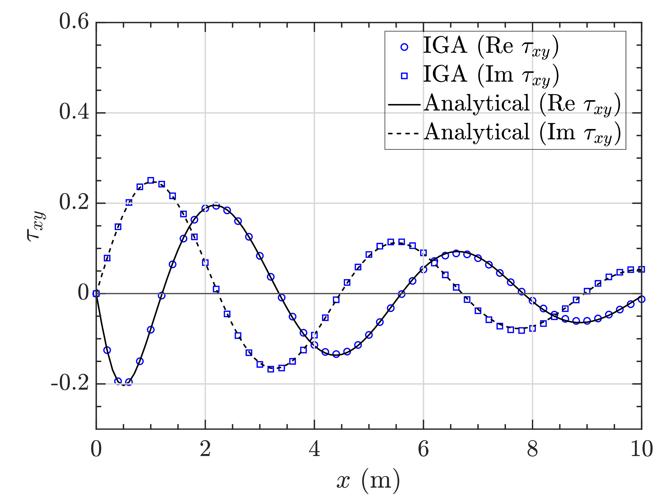

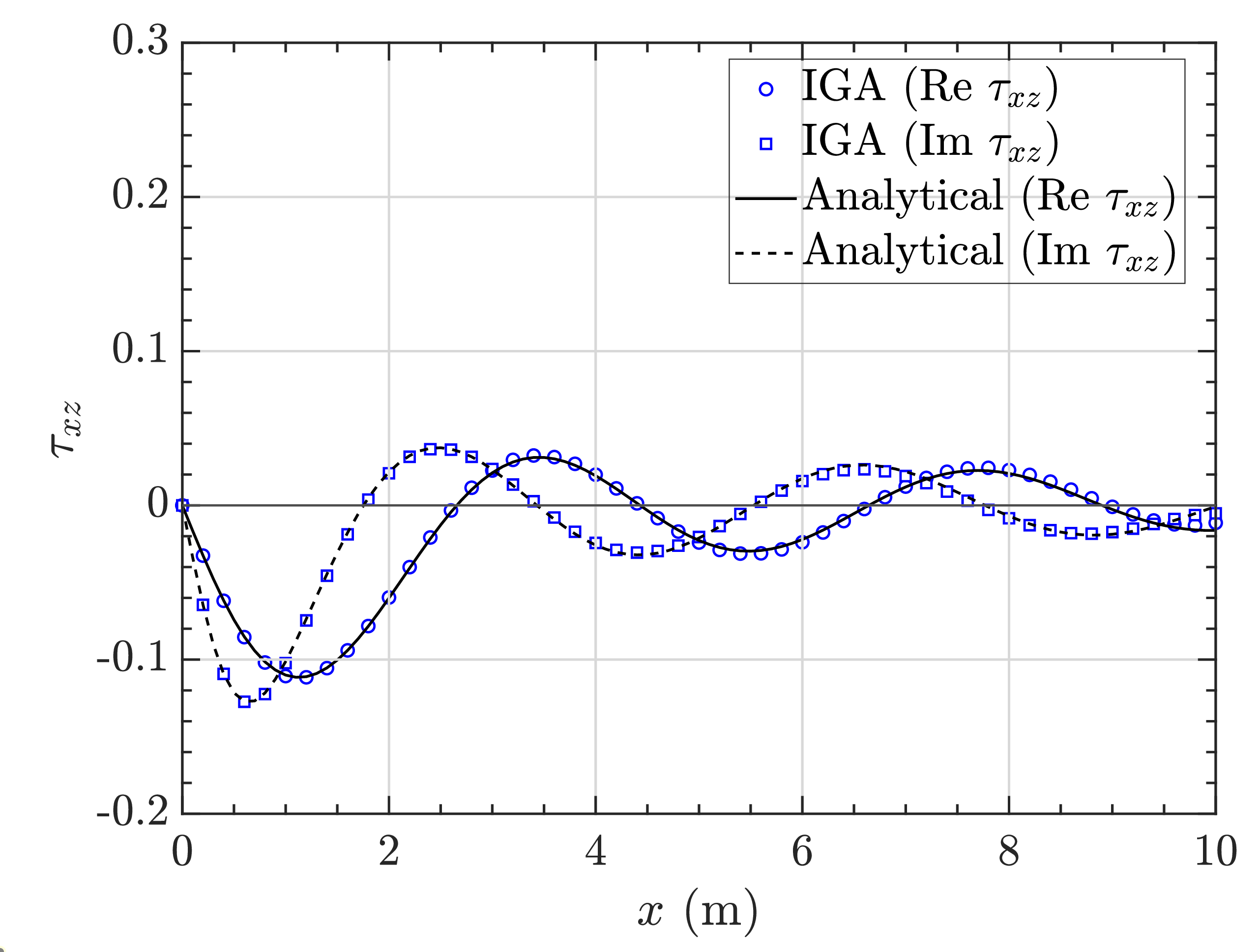
Figure 8: Frequency-domain stresses for \(f=32~\mathrm{Hz}\), no self-oscillation, \(c_{\mathrm{load}}=120~\mathrm{m/s}\), and \(\zeta=0.05\), plotted along the \(x\)-axis at \(y=1~\mathrm{m}\). (a) \(\sigma_{xx}\); (b) \(\sigma_{yy}\); (c) \(\sigma_{zz}\); (d) \(\tau_{xy}\); (e) \(\tau_{yz}\); (f) \(\tau_{xz}\)..
4.1.2 Assessment of the radiation boundary and radial decay↩︎
The high-frequency verification in the previous subsection primarily assesses the bounded-domain discretization because the artificial boundary is comparatively remote in terms of wavelength. The present subsection instead defines a default realization of the radiation treatment and a reproducible screening procedure for detecting sensitivity to the selected exterior setting without access to an analytical solution. A controlled mixed-wave calibration is then considered separately to quantify the additional accuracy attainable within its verified parameter envelope.
4.1.2.1 Reference-free all-S boundary assessment
The assessment uses a fixed all-S exterior model as the default radial realization of the trace-space formulation in Section 3.3. The same S-wave-informed radial family is applied on all artificial-boundary segments, and its reference decay coefficient is scaled as \[\alpha_{S,q}=\beta_S\alpha_{S,q}^{\mathrm{ref}}, \qquad \beta_S=1\quad\text{by default}, \label{eq:allS95default}\tag{69}\] where \(q\) identifies a boundary segment and \(\alpha_{S,q}^{\mathrm{ref}}\) is given explicitly by Eq. 43 . In the present rectangular domains, \(L_q=R\) for a lateral segment and \(L_q=H\) for a lower segment. The dimensionless exterior frequency is \[\eta_S=\frac{\omega R}{c_{S,\infty}}, \label{eq:etaS95alpha}\tag{70}\] where \(R\) is the truncation radius and \(c_{S,\infty}\) is the shear-wave speed of the exterior material. This definition depends on the far field rather than on local inclusions inside the bounded domain. The all-S realization removes the need to prescribe an a priori Rayleigh/S-wave partition of the artificial boundary and leaves only one radial family to be checked.
For problems without an analytical reference, boundary adequacy is tested by repeating the solution for the fixed perturbation set \[\mathcal{B}=\{0.75,1.00,1.25\}. \label{eq:beta95perturbation95set}\tag{71}\] Let \(x_r=0,0.2,\ldots,4~\mathrm{m}\) and \(y_r=1~\mathrm{m}\) denote the fixed physical receivers used in this audit. The response vector stacks the vertical component and the sign-aligned horizontal component at these receivers, \[\mathbf{u}_{\beta} = \left[ \tilde{u}_{v}(x_1,y_1;\beta),\ldots,\tilde{u}_{v}(x_{N_r},y_{N_r};\beta), \tilde{u}_{h}^{\mathrm{sa}}(x_1,y_1;\beta),\ldots,\tilde{u}_{h}^{\mathrm{sa}}(x_{N_r},y_{N_r};\beta) \right]^T, \label{eq:boundary95response95vector}\tag{72}\] where “sa” denotes the fixed sign transformation required to reconcile the analytical and numerical transverse-axis conventions. The dimensionless radial-sensitivity indicator is defined as \[I_{\beta} = \max_{\substack{\beta_a,\beta_b\in\mathcal{B}\\\beta_a<\beta_b}} \frac{\|\mathbf{u}_{\beta_a}-\mathbf{u}_{\beta_b}\|_2}{\|\mathbf{u}_{\beta=1}\|_2}. \label{eq:beta95spread}\tag{73}\]
| Varied factor | Tested settings | \(I_{\beta}\) | Principal observation |
|---|---|---|---|
| Exterior frequency | \(f=2,5,8\) Hz; \(\eta_S=1.257,3.142,5.027\) | \(0.2853,0.0825,0.0118\) | Sensitivity decreases with exterior distance measured in wavelengths; the 2-Hz case triggers enlargement. |
| Load-speed ratio | \(M_S=0.6,0.9,1.2\) at \(\eta_S=\pi\) | \(0.0002,0.0825,0.3153\) | The default is insensitive in the sub-shear cases; the super-shear case triggers enlargement. |
| Poisson ratio | \(\nu=0.15,0.25,0.35,0.45\) | \(0.1191\)–\(0.0448\) | All \(I_{\beta}\) values remain below the preliminary sensitivity screen; \(I_D\) is still required. |
| Damping ratio | \(\zeta=0.01,0.05,0.10\) | \(0.1323\)–\(0.0392\) | Sensitivity decreases as material attenuation increases. |
| Boundary aspect ratio | \(H/R=0.5,1,2\) | \(0.2157,0.0825,0.0265\) | A shallow lower boundary is detected directly by the indicator. |
| Similarity scaling | \(c_S=80,100,120\) m/s at fixed \(\eta_S\) and \(M_S\) | \(0.082481\) in all cases | Dimensionless invariance is recovered to numerical precision. |
| Trace resolution | \(8\times4\), \(12\times6\), \(16\times8\) | \(0.0824\)–\(0.0825\) | The indicator is independent of trace refinement over the tested range. |
| NURBS degree | quadratic and cubic trace bases | \(0.08248,0.08249\) | The diagnostic is unchanged by degree elevation. |
| Near-field contrast | homogeneous, stiff inclusion, local soft layer | \(0.0825,0.0319,0.1852\) | The local soft layer triggers boundary enlargement; exterior material remains unchanged. |
3pt
The heterogeneous holdout uses the same \(R=H=10~\mathrm{m}\) exterior and changes only the bounded material. The stiff inclusion occupies \(2\leq x\leq5~\mathrm{m}\) and \(3\leq y\leq6~\mathrm{m}\), with \(E_{\mathrm{inc}}/E_{\infty}=5\), \(\nu_{\mathrm{inc}}=0.20\), and \(\rho_{\mathrm{inc}}/\rho_{\infty}=1.20\). The local soft layer occupies \(0\leq x\leq7~\mathrm{m}\) and \(0\leq y\leq3~\mathrm{m}\), with \(E_{\mathrm{soft}}/E_{\infty}=0.35\), \(\nu_{\mathrm{soft}}=0.35\), and \(\rho_{\mathrm{soft}}/\rho_{\infty}=0.90\).
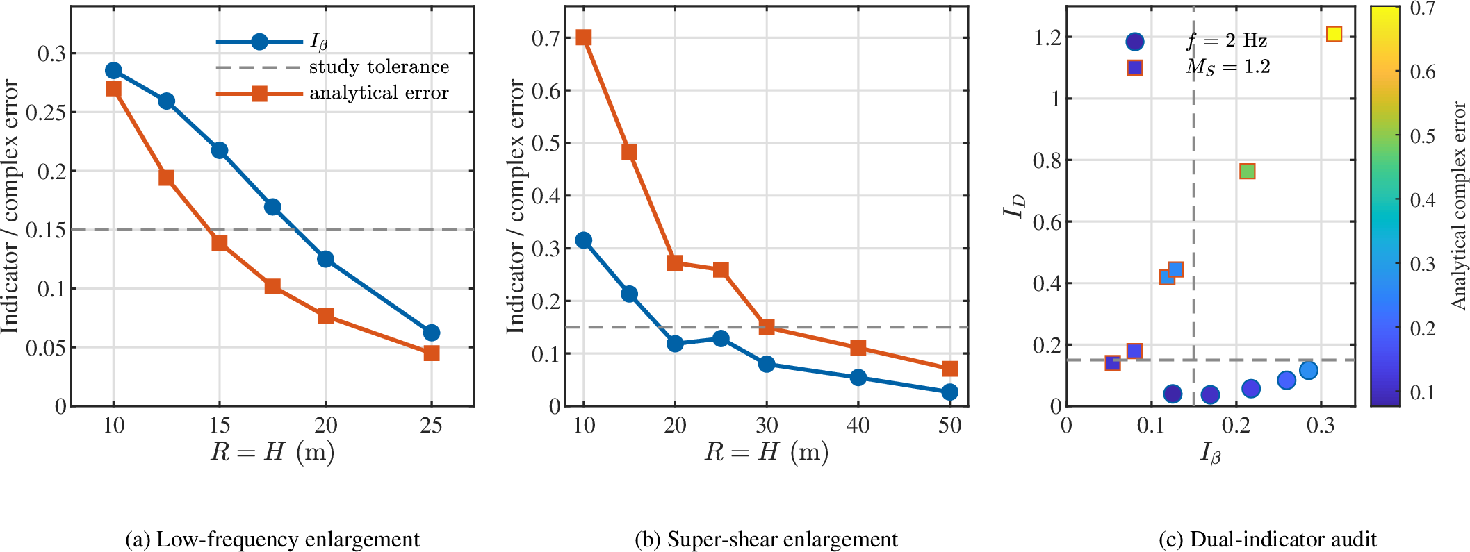
The subscript \(\beta\) indicates that the sensitivity is evaluated by perturbing \(\beta_S\); \(I_{\beta}\) is not a material or infinite-element parameter. A small value shows that the response is stationary with respect to a finite perturbation of the radial decay. A second, independent check complements this decay-parameter test by comparing two successive near-field domains \(D_j\) and \(D_{j+1}\) while preserving the physical receiver locations and the resolution per unit length. Here \(\mathbf{u}_{D_j}\) has exactly the component ordering and receiver coordinates in Eq. 72 , is evaluated with \(\beta_S=1\), and differs only through the domain \(D_j\): \[I_D^{(j)} = \frac{\|\mathbf{u}_{D_{j+1}}-\mathbf{u}_{D_j}\|_2}{\|\mathbf{u}_{D_{j+1}}\|_2}. \label{eq:domain95change95indicator}\tag{74}\] Neither \(I_{\beta}\) nor \(I_D\) uses the analytical solution. The working value \(0.15\) is applied to both indicators in the present screening study and is audited below against the true complex displacement error. The two tests answer different questions: \(I_{\beta}\) detects decay-parameter sensitivity on a fixed domain, whereas \(I_D\) detects residual dependence on boundary placement even when the response happens to be stationary with respect to \(\beta_S\).
Table 1 establishes parameter robustness of the all-S model, but parameter robustness is not equivalent to accuracy. The indicator pair is therefore calibrated against the closed-form half-space solution using ordered domain-enlargement sequences at low frequency, at super-shear speed, and for the lower-boundary depth. The analytical response is used only in this audit and is not used to choose \(\beta_S\), \(I_{\beta}\), or \(I_D\).
| Case and successive domains | \(I_{\beta}^{(j)}\) | \(I_D^{(j)}\) | \(e_j\) | \(e_{j+1}\) | Indicator result at \(D_j\) |
|---|---|---|---|---|---|
| \(f=2\) Hz, \(R_j/R_{j+1}=10/12.5\) m | 0.2853 | 0.1164 | 0.2700 | 0.1941 | enlarge |
| \(f=2\) Hz, \(R_j/R_{j+1}=20/25\) m | 0.1251 | 0.0400 | 0.0765 | 0.0450 | dual screen met |
| \(M_S=1.2\), \(R_j/R_{j+1}=10/15\) m | 0.3153 | 1.2096 | 0.7007 | 0.4825 | enlarge |
| \(M_S=1.2\), \(R_j/R_{j+1}=20/25\) m | 0.1186 | 0.4191 | 0.2721 | 0.2594 | enlarge by \(I_D\) |
| \(M_S=1.2\), \(R_j/R_{j+1}=40/50\) m | 0.0544 | 0.1400 | 0.1109 | 0.0712 | dual screen met |
| \(H_j/H_{j+1}=10/12.5\) m | 0.0825 | 0.0109 | 0.0612 | 0.0541 | dual screen met |
4pt
Figure 9 and Table 2 demonstrate why both checks are retained. In the 2-Hz sequence, \(I_{\beta}\) and the true error decrease together from \((0.2853,0.2700)\) at \(R=10~\mathrm{m}\) to \((0.0624,0.0450)\) at \(R=25~\mathrm{m}\). The super-shear case supplies the more demanding counter-test: at \(R=20~\mathrm{m}\), \(I_{\beta}=0.1186\) alone would indicate apparent stability although the true error remains \(0.2721\); the large value \(I_D=0.4191\) identifies this false acceptance. For the successive domains \(R_j=40~\mathrm{m}\) and \(R_{j+1}=50~\mathrm{m}\), the indicators are \(I_{\beta}=0.0544\) and \(I_D=0.1400\), while the corresponding analytical errors are \(0.1109\) and \(0.0712\). Across the tested enlargement sequences, cases satisfying both \(I_{\beta}\leq0.15\) and \(I_D\leq0.15\) have a current-domain analytical error no larger than \(0.1109\), while the enlarged-domain error is no larger than \(0.0712\). The value \(0.15\) is therefore used as an empirically audited boundary-sensitivity screening level for this study, with the tested dual-pass cases reaching approximately \(11\%\) or smaller analytical error on the current domain.
The all-S workflow is consequently staged but reference free: compute the fixed \(\beta_S=1\) response and its three-point perturbation, then repeat the final candidate on one enlarged domain. The boundary placement is classified as insensitive under the present screen only when both Eqs. 73 and 74 satisfy the study values; otherwise, the near field is enlarged without reference-based retuning. This dual check preserves the simplicity of the all-S realization while guarding against a radial family that is insensitive to \(\beta_S\) but still affected by boundary placement. Accuracy is established separately by an analytical benchmark or conventional discretization refinement whenever such evidence is available.
4.1.2.2 Controlled mixed-wave calibration
To quantify the additional accuracy that radial calibration can provide in a compact domain, the mixed-wave calibration developed in this work is retained as a controlled secondary experiment. It assigns Rayleigh- and S-wave-informed radial functions to the surface-adjacent and remaining exterior segments, respectively, and scales their reference decay coefficients by \(\beta_R^{\mathrm{cal}}(\eta_S)\) and \(\beta_S^{\mathrm{cal}}(\eta_S)\). Frequency-by-frequency minimization of the sign-aligned complex displacement error in the homogeneous reference model is summarized by \[\beta_R^{\mathrm{cal}}(\eta_S)= \begin{cases} 0, & 0.314\leq\eta_S<0.628,\\ \max\!\left(0,-0.0644\eta_S^2+0.8014\eta_S-0.5029\right), & 0.628\leq\eta_S\leq5.027, \end{cases} \label{eq:betaR95calibrated}\tag{75}\] and \[\beta_S^{\mathrm{cal}}(\eta_S)= \begin{cases} 2.364\eta_S-0.0105, & 0.314\leq\eta_S<0.628,\\ 0.0206\eta_S^3-0.2028\eta_S^2+0.9636\eta_S+0.9325, & 0.628\leq\eta_S\leq5.027. \end{cases} \label{eq:betaS95calibrated}\tag{76}\] These curves compactly represent the calibration model and are not additional constitutive parameters of NBIEM. At the two diagnostic points with \(\eta_S>5.027\), the polynomial branches are evaluated by direct continuation solely to inspect behavior beyond the calibration interval; their range of claimed validity is not extended.

Figure 10 compares the absolute complex errors of the two radial treatments. Both improve rapidly as \(\eta_S\) increases and reach errors of order \(10^{-2}\) near the upper part of the calibration interval. The calibrated rule provides an additional reduction in the compact-domain low-frequency cases, whereas the separation between the curves becomes small once the all-S response is already weakly dependent on radial decay. The zero-frequency endpoint is represented numerically by the lowest positive frequency sample and is used only to close the discrete spectrum. The calibration is therefore retained as an optional accuracy enhancement within its declared model, rather than as a replacement for the transferable all-S workflow.
4.1.2.3 Controlled hybrid time reconstruction
The practical time-domain influence of the low-frequency radial treatment is assessed using controlled inverse reconstructions over \(0\)–\(200~\mathrm{Hz}\) and \(0\)–\(400~\mathrm{Hz}\). Within the nominal \(0\)–\(8~\mathrm{Hz}\) interval, the computed all-S and calibrated mixed-wave NBIEM spectra are retained, whereas both reconstructions use the same analytical half-space spectrum at higher frequencies. At the zero-frequency endpoint, the lowest positive frequency sample supplies the numerical endpoint value. This construction directly isolates whether the low-frequency radial-rule difference remains significant in conventional broadband ground-response reconstructions. The common cutoff is increased from \(20\) to \(400~\mathrm{Hz}\) to examine convergence with reconstruction bandwidth.
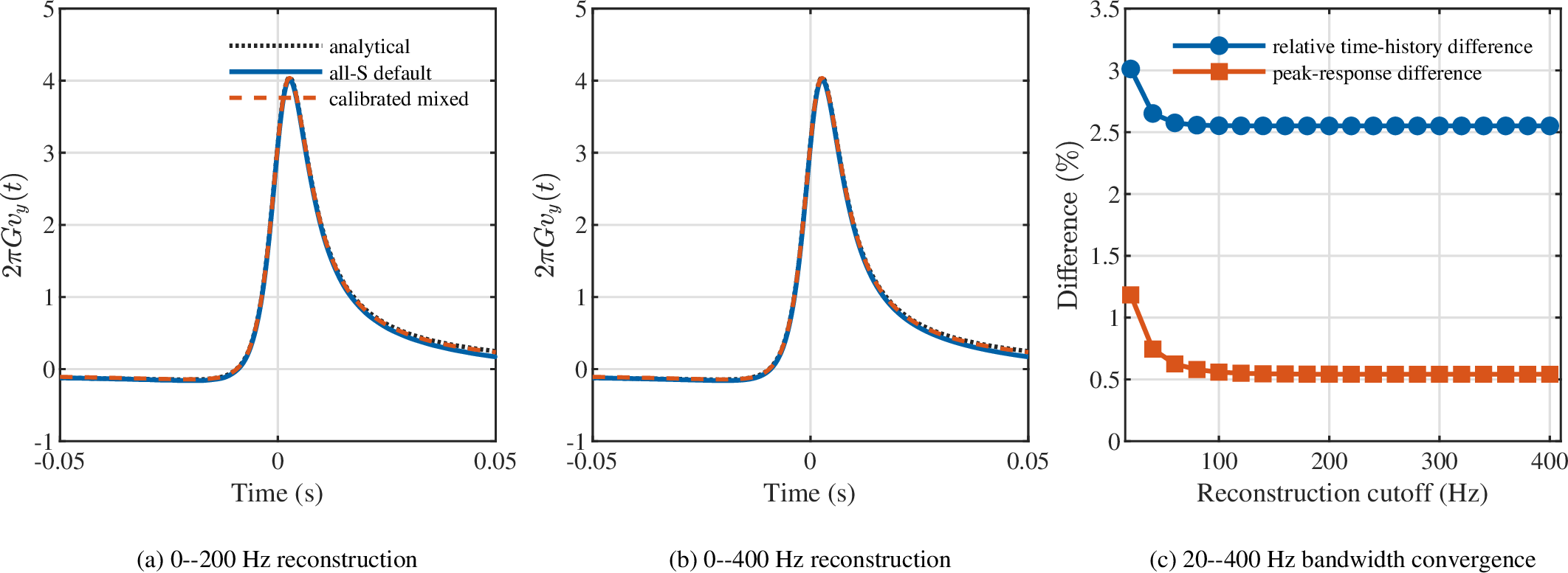
Figure 11 (a)–(b) shows that the all-S and calibrated mixed-wave histories are nearly coincident in both broadband reconstructions. For the reconstruction with a \(200\)-Hz cutoff, their relative time-history difference is \(2.55\%\), the peak-response difference is \(0.54\%\), the maximum pointwise difference is \(1.60\%\), and the correlation coefficient is \(0.9999\); the corresponding \(400\)-Hz-cutoff values are unchanged to the reported precision. Figure 11 (c) further shows that the difference measures become essentially stationary once the reconstruction bandwidth exceeds approximately \(80~\mathrm{Hz}\).
A separate direct same-model Fourier-grid test holds each radial treatment fixed and compares its reconstructed history with the \(\Delta f=0.05~\mathrm{Hz}\) result. Every NBIEM value on the requested grids within \(0\)–\(8~\mathrm{Hz}\) is solved directly; no interpolated value is introduced as a new NBIEM sample. For \(\Delta f=0.25\), \(0.125\), and \(0.10~\mathrm{Hz}\), the all-S grid errors are \(1.03\%\), \(0.39\%\), and \(0.26\%\), while the calibrated mixed-wave grid errors are \(1.75\%\), \(0.65\%\), and \(0.44\%\). These are same-model spectral-sampling errors of the controlled hybrid reconstruction, unlike the all-S/mixed-wave differences shown in Fig. 11. Thus, within the present controlled hybrid reconstructions, the calibrated rule improves the complex low-frequency response in Fig. 10, but its influence on the broadband histories is limited; the fixed all-S realization preserves the principal waveform and peak response without calibration-dependent boundary partitioning.
The calibration and robustness results serve different purposes. Figure 10 establishes the accuracy gain attainable when a trusted reference is available, whereas Fig. 9 supports the complementary reference-free checks used when transferring the method to new configurations. The calibrated rule is therefore retained as a controlled enhancement within its declared envelope, while the all-S setting and Eqs. 73 –74 define the transferable default workflow.
4.1.2.4 High-frequency phase and spectral audits
Where an analytical response is available, accuracy is reported using the vertical displacement and a sign-aligned horizontal displacement. The analytical horizontal component follows the opposite transverse-axis convention to the numerical model; this deterministic coordinate transformation is applied before any combined norm or phase comparison. The resulting evidence is organized by error source in Table 3, rather than summarized by a single undifferentiated displacement error.
The amplitude-weighted phase error used here and in the following subsection is \[e_{\phi} = \left[ \frac{ \displaystyle\sum_{m\in\mathcal{M}}\sum_{r\in\mathcal{S}} w_{mr}\left(\phi^{\mathrm{num}}_m(\mathbf{x}_r)-\phi^{\mathrm{ana}}_m(\mathbf{x}_r)\right)^2 }{ \displaystyle\sum_{m\in\mathcal{M}}\sum_{r\in\mathcal{S}}w_{mr} } \right]^{1/2}, \qquad w_{mr}=\left|\tilde{u}^{\mathrm{ana}}_m(\mathbf{x}_r)\right|^2, \label{eq:method95phase95error}\tag{77}\] where \(\phi=\operatorname{unwrap}(\arg\tilde{u})\) is evaluated separately for each displacement component along the ordered receiver profile before the component vectors are stacked. The weighting suppresses ill-conditioned phases near zeros of the analytical response.
The high-frequency discretization is audited independently over \(10\)–\(32~\mathrm{Hz}\) using five frequencies and three meshes that maintain approximately 8, 12, and 16 points per S wavelength. Figure 12 shows that the finest-mesh amplitude error is \(0.87\%\) at \(10~\mathrm{Hz}\) and below \(0.2\%\) from \(15\) to \(32~\mathrm{Hz}\), whereas the amplitude-weighted phase error increases with frequency and changes little under proportional mesh refinement. This pattern is consistent with the acoustic IGA literature on pollution-type phase accumulation and high-frequency wave behavior [20], but the audit does not uniquely separate that contribution from residual exterior-model error, radial approximation, systematic phase offset, or receiver-distance effects. It therefore provides a high-frequency phase diagnostic rather than a single-cause attribution, and prevents the \(2\)–\(8~\mathrm{Hz}\) method comparison from being used as the sole evidence for high-frequency behavior.

For inverse reconstruction, frequency and longitudinal-wavenumber sampling are not independent because Eq. 40 gives \[\Delta k=\frac{\Delta\omega}{c_{\mathrm{load}}} =\frac{2\pi\Delta f}{c_{\mathrm{load}}}. \label{eq:wavenumber95sampling}\tag{78}\] Thus every frequency-grid refinement reported above simultaneously refines the moving-load wavenumber grid; a separate \(k\) quadrature is not used for a single moving harmonic component.
| Numerical contribution | Isolation strategy | Numerical evidence | Assessment used in this work |
|---|---|---|---|
| Cross-sectional discretization | Repeat the baseline case with coarse, reference, and fine NURBS meshes at fixed exterior model. | Total sign-aligned errors \(0.0637\), \(0.0612\), and \(0.0613\) demonstrate mesh stationarity of the reported response measure. | Resolve the minimum wavelength and verify nested-mesh stationarity. |
| Spline degree and boundary quadrature | Elevate the quadratic trace to cubic and repeat the cubic result with 3, 4, and 5 Gauss points per knot span. | Degree-elevation errors are \(0.0611907\) and \(0.0612118\); the cubic response and \(I_{\beta}\) change by less than \(1.1\times10^{-9}\) from 3 to 5 points. | Use \(n_g=\max(3,p_b+1)\) in production and confirm degree robustness. |
| Radiation boundary | Perturb \(\beta_S\) and independently enlarge the bounded domain, then audit both indicators against the analytical error. | The \(R=20\) m super-shear apparent pass by \(I_{\beta}\) is rejected by \(I_D=0.4191\); for \(R_j/R_{j+1}=40/50\) m, the error falls from \(0.1109\) to \(0.0712\). | Apply both \(I_{\beta}\) and \(I_D\) for the sensitivity screen; verify accuracy separately. |
| Radial integration | Compare Eq. [eq:radial95moment95exact] and its derivative-moment matrix with direct adaptive complex integration on \([0,\infty)\). | No finite cutoff or user variable transform; relative/absolute tolerances \(10^{-12}/10^{-14}\) give maximum mass/stiffness residuals \(1.58\times10^{-16}/1.42\times10^{-16}\). | Production radial moments are analytical; audit residuals use the relative Frobenius norm. |
| High-frequency phase behavior | Maintain 8, 12, and 16 points per wavelength over five frequencies from 10 to 32 Hz. | Finest-mesh amplitude error is \(0.12\)–\(0.87\%\); phase growth is weakly affected by proportional mesh refinement. | Treat the result as consistent with, but not a unique identification of, accumulated phase pollution. |
| Spectral sampling | Directly solve every low-frequency NBIEM node on each fixed-model grid and map it to \(k\) through Eq. [eq:wavenumber95sampling]. | Against \(\Delta f=0.05\) Hz, all-S errors at \(0.25/0.125/0.10\) Hz are \(1.03/0.39/0.26\%\); mixed-wave errors are \(1.75/0.65/0.44\%\). | Verify direct same-model \(\Delta f\) convergence; \(\Delta k\) follows simultaneously. |
3pt
The assessment results support a reproducible operational hierarchy. The fixed all-S setting is used without reference-based tuning, and candidate boundary placements are screened through both decay-parameter stability and domain-enlargement stability. This separates the transferable workflow from the calibrated mixed-wave accuracy enhancement while leaving the NURBS-trace coupling unchanged.
4.1.3 Comparison with alternative boundary treatments↩︎
To further assess the proposed NBIEM, its accuracy is compared with two boundary-treatment strategies that are closest to the present formulation. The conventional finite/infinite element formulation (FEM/IEM) is selected as the classical 2.5D moving-load reference because it uses the same finite/infinite-element radiation philosophy on a low-order finite-element trace [8]. The scaled-boundary isogeometric analysis formulation (IGA/SBIGA) is selected as the spline-based reference because it represents the NURBS-based counterpart of the FEM–SBFEM route for 2.5D train-induced vibration problems [26]. Perfectly matched layers provide another important family of artificial boundaries, and displacement-based 2.5D PML formulations have also been developed [17]. A PML baseline is not used here because its accuracy depends on absorbing-layer thickness, stretching or attenuation functions, and layer discretization, whereas the present comparison focuses on boundary-attached exterior discretizations coupled directly to the boundary trace. The selected cases sample the low-to-intermediate frequency band in which the artificial-boundary treatment remains visible; at higher frequencies, the dependence on the particular admissible boundary treatment decreases and the response becomes increasingly governed by the near-field discretization. The comparison is conducted under matched physical cross-sectional partitions. The resulting difference in global degrees of freedom is an intrinsic consequence of the respective approximation spaces and is therefore retained as part of the performance assessment.
This subsection compares both accuracy and the core cost of the unbounded-domain treatment. Accuracy is assessed over five matched refinement levels, whereas the timing sweep uses a dense sequence of meshes and supplemental large-mesh points so that the cost growth is represented directly rather than inferred from a few widely separated partitions. The reference-free all-S realization is adopted throughout the cross-method comparison and the subsequent engineering applications, without frequency-by-frequency optimization.
The displacement accuracy is first measured by the normalized complex \(L_2\) error \[e_{L_2} = \left[ \frac{ \displaystyle\sum_{m\in\mathcal{M}}\sum_{q\in\mathcal{S}} \left| \tilde{u}^{\mathrm{num}}_m(\mathbf{x}_q) - \tilde{u}^{\mathrm{ana}}_m(\mathbf{x}_q) \right|^2 }{ \displaystyle\sum_{m\in\mathcal{M}}\sum_{q\in\mathcal{S}} \left| \tilde{u}^{\mathrm{ana}}_m(\mathbf{x}_q) \right|^2 } \right]^{1/2}, \label{eq:method95L295error}\tag{79}\] where \(\mathcal{M}\) denotes the selected displacement components and \(\mathcal{S}\) denotes the sampling points along the verification profiles. Since the responses are complex-valued frequency-response functions, Eq. 79 accounts for both real and imaginary parts. The metric is a discrete relative \(\ell_2\) error over the receiver samples, denoted by \(e_{L_2}\) for consistency with the figures; no quadrature weights are introduced in this profile-based comparison.
For wave-propagation problems, phase accuracy is assessed with the amplitude-weighted metric \(e_{\phi}\) defined previously in Eq. 77 .
Fig. 13 shows a smooth improvement of NBIEM as the dimensionless frequency increases. In this comparison, NBIEM uses the reference-free fixed all-S radial realization described in the preceding boundary-assessment study. At the representative matched partition \(N_e=144\), NBIEM reduces the \(2\)-Hz displacement error from \(0.3642\) for FEM/IEM to \(0.2913\), while IGA/SBIGA gives \(e_{L_2}=0.0261\). At \(6~\mathrm{Hz}\), NBIEM further reduces the FEM/IEM error from \(0.0854\) to \(0.0458\) and approaches the IGA/SBIGA value of \(0.0357\). The NBIEM and IGA/SBIGA curves then become nearly coincident: at \(8~\mathrm{Hz}\) the errors are \(0.0407\) for NBIEM, \(0.0398\) for IGA/SBIGA, and \(0.1167\) for FEM/IEM, while at \(12~\mathrm{Hz}\) NBIEM and IGA/SBIGA both give approximately \(0.0480\), compared with \(0.0685\) for FEM/IEM. The refinement curves therefore show that NBIEM provides a favorable displacement accuracy–cost balance from the intermediate-frequency cases onward, while retaining a simpler far-field construction.
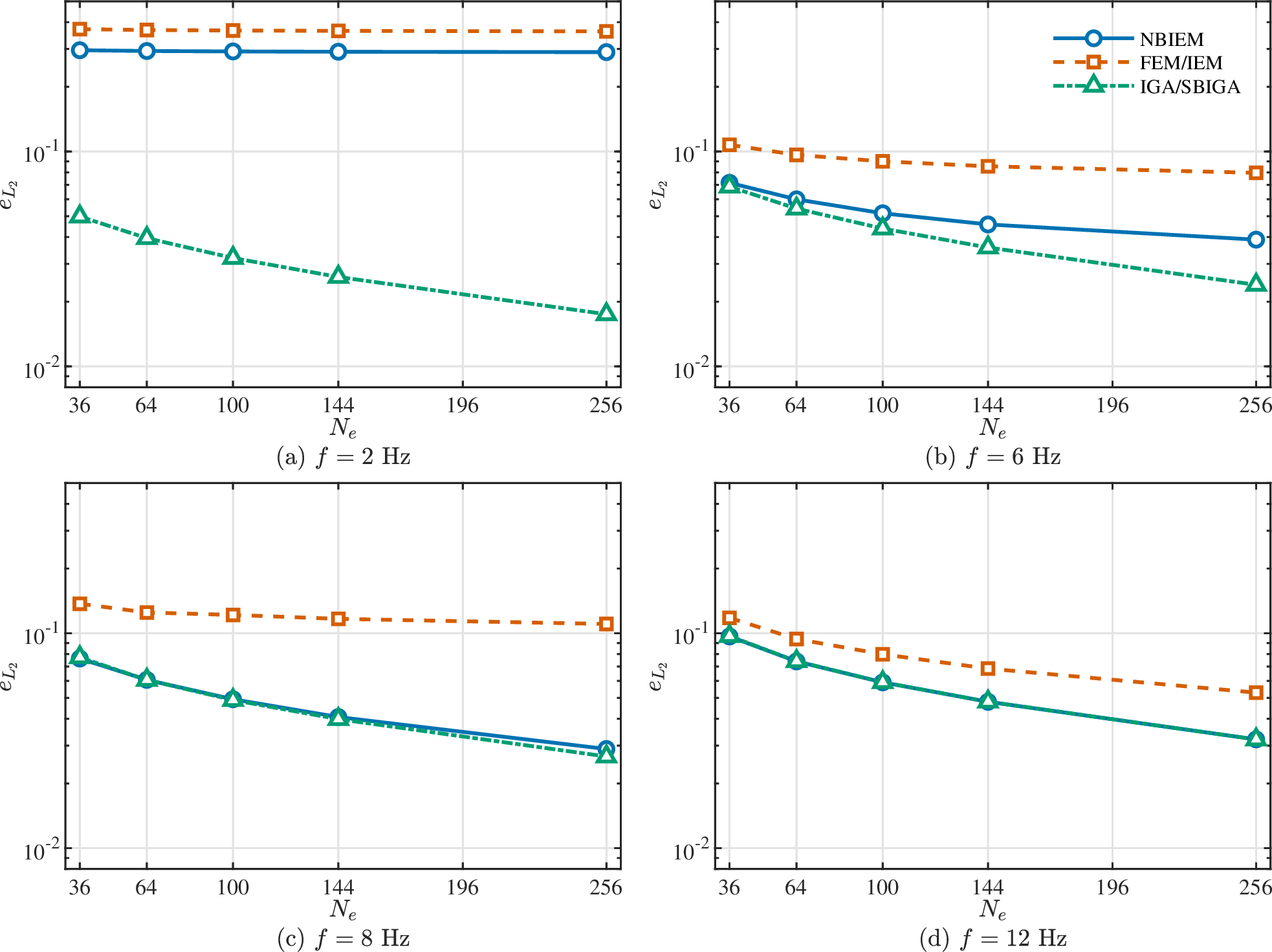
The phase comparison in Fig. 14 confirms the frequency-dependent improvement of NBIEM over the investigated range. At \(N_e=144\), the \(2\)-Hz NBIEM phase error is \(14.48^{\circ}\), while FEM/IEM and IGA/SBIGA give \(10.63^{\circ}\) and \(0.28^{\circ}\), respectively. As the frequency increases, NBIEM rapidly approaches the IGA/SBIGA result and improves on the conventional FEM/IEM exterior treatment. At \(6~\mathrm{Hz}\), NBIEM reduces the FEM/IEM phase error from \(3.03^{\circ}\) to \(0.86^{\circ}\) and follows the IGA/SBIGA value of \(0.46^{\circ}\). At \(8~\mathrm{Hz}\), the corresponding errors are \(0.61^{\circ}\), \(4.55^{\circ}\), and \(0.54^{\circ}\) for NBIEM, FEM/IEM, and IGA/SBIGA, respectively. At \(12~\mathrm{Hz}\), all three methods show small phase errors, with \(0.72^{\circ}\) for NBIEM, \(0.95^{\circ}\) for FEM/IEM, and \(0.69^{\circ}\) for IGA/SBIGA. The combined amplitude and phase results therefore support a frequency-aware accuracy–cost interpretation: at \(2~\mathrm{Hz}\), NBIEM improves the combined displacement error relative to FEM/IEM but remains more phase-sensitive and less accurate than IGA/SBIGA; from \(6~\mathrm{Hz}\) onward, its phase response approaches the IGA/SBIGA result while retaining a substantially simpler and less expensive far-field construction.
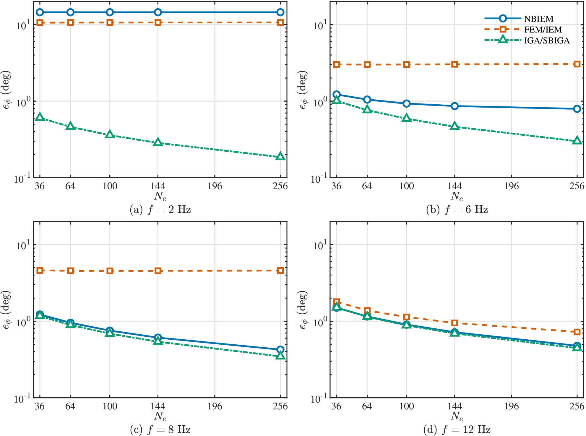
Table 4 gives a representative equal-partition comparison at \(8~\mathrm{Hz}\). At the same physical partition \(N_e=144\), NBIEM and IGA/SBIGA have the same number of global displacement degrees of freedom and nearly the same displacement and phase errors, while the NBIEM wall-clock core time is much lower because no scaled-boundary far-field dynamic stiffness is solved. FEM/IEM uses more degrees of freedom under the same partition and remains less accurate for this case.
| Method | \(N_{\mathrm{dof}}\) | \(e_{L_2}\) | \(e_{\phi}\) (deg) | Core wall-clock time (s) |
|---|---|---|---|---|
| FEM/IEM | 1443 | 0.1167 | 4.55 | 0.140 |
| NBIEM | 588 | 0.0407 | 0.61 | 0.023 |
| IGA/SBIGA | 588 | 0.0398 | 0.54 | 168.1 |
The computational cost of the three methods is further compared in Fig. 15. The timings were obtained from the same MATLAB implementation using tic/toc measurements and sparse direct
linear solves. To isolate the cost most directly affected by the unbounded-domain formulation, the reported core wall-clock time includes exterior-matrix construction, dynamic-system solution, and response extraction. Geometry and mesh generation,
analytical-reference evaluation, and near-field matrix assembly are excluded from all three curves. All methods were evaluated in the same computational environment, and the reported wall-clock times are intended for relative performance comparison.
As shown in Fig. 15, FEM/IEM is inexpensive for relatively small meshes, but its computational cost increases rapidly as the mesh is refined. This is mainly due to the faster growth of the global degrees of freedom and the resulting increase in linear-solve cost. IGA/SBIGA provides a strong low-frequency comparison baseline, but it requires a much higher computational cost even for moderate mesh sizes because the scaled-boundary far-field dynamic stiffness has to be constructed and solved. In contrast, NBIEM maintains a much lower wall-clock time over the tested mesh range. In particular, at larger element counts, NBIEM remains substantially faster than FEM/IEM, while also avoiding the high boundary-assembly cost of IGA/SBIGA.
At \(N_e=144\), NBIEM uses 588 degrees of freedom, approximately \(40.7\%\) of the 1443 degrees of freedom in FEM/IEM, and its measured core wall-clock time is \(0.023~\mathrm{s}\), compared with \(0.140~\mathrm{s}\) for FEM/IEM and \(168.1~\mathrm{s}\) for IGA/SBIGA. At \(N_e=256\), the respective times are \(0.049\), \(0.485\), and \(761.6~\mathrm{s}\). The supplemental large-mesh timing sweep gives the same growth trend: at matched partitions with \(N_e=400\) and \(576\), the NBIEM core wall-clock times remain \(0.132\) and \(0.200~\mathrm{s}\), whereas FEM/IEM increases to \(0.901\) and \(2.209~\mathrm{s}\); at the largest FEM/IEM timing point, \(N_e=900\), the corresponding core wall-clock time reaches \(6.588~\mathrm{s}\). On the present implementation and hardware, NBIEM is therefore already about one order of magnitude faster than FEM/IEM at moderate-to-large partitions, while also avoiding the iterative far-field dynamic-stiffness construction that dominates IGA/SBIGA. Together with the low-to-intermediate-frequency accuracy results, these measurements establish the principal advantage of the proposed formulation: a frequency-dependent accuracy–cost balance for repeated frequency-domain simulations, with clear low-frequency sensitivity and behavior close to IGA/SBIGA from the representative medium-frequency cases onward.

This section verifies the proposed 2.5D NURBS-trace infinite-element formulation through comparisons with closed-form solutions over a range of moving-load speeds, including cases with a nonzero self-oscillation frequency. The displacement and stress results show that the formulation reproduces both primary response quantities and derivative-dependent fields in the tested settings. Under matched cross-sectional partitions, NBIEM gives a frequency-dependent accuracy–cost trade-off: it improves the displacement error relative to classical FEM/IEM and approaches IGA/SBIGA from the intermediate-frequency cases onward, while using substantially fewer globally independent degrees of freedom than the corresponding FEM/IEM discretization. Compared with IGA/SBIGA, it retains the NURBS-based near-field discretization but avoids the repeated construction of a scaled-boundary far-field dynamic stiffness, leading to a lower-cost exterior-domain treatment in the reported implementation. Unlike PML-based formulations, NBIEM does not require an additional absorbing layer or associated layer-parameter tuning, and unlike FE–BE coupling, it does not rely on problem-specific Green’s functions or boundary-integral evaluation. The assessed all-S realization is therefore adopted in the subsequent single-frequency parametric and engineering-oriented investigations.
4.2 Effect of treated depth \(h\) in a soft-interlayer subgrade: comparison between the coupled pavement-subgrade model and the overall layered model↩︎
The proposed computational framework is applied to the dynamic analysis of layered pavement systems. For pavements constructed on a zero-fill foundation, many numerical studies adopt an overall layered model in which the pavement and supporting ground are treated as laterally unbounded. This representation is convenient for model construction and solution, while the coupled model introduced below represents the finite pavement width explicitly. In the present study, two structural representations are considered and their applicability is distinguished by their geometric description. As illustrated in Fig. 16, the overall layered model (Fig. 16 (a)) neglects the finite pavement width, whereas the coupled model (Fig. 16 (b)) explicitly incorporates the actual pavement width and therefore provides a more faithful description of the cross-sectional geometry.
This section compares the two models in terms of the dynamic responses under different transverse load locations across the pavement width. In addition, the influence of a soft interlayer embedded in the foundation is examined for both modeling strategies to assess its effect on the coupled pavement–subgrade response. The material properties of each layer are summarized in Table 5.


Figure 16: Isogeometric discretizations of the two modeling strategies. (a) Overall layered model; (b) Coupled pavement-subgrade model. Blue circles denote control points and black lines indicate NURBS elements..
| Layer | \(E\) (MPa) | \(\rho\) (kg/m\(^{3}\)) | \(\nu\) (-) | \(\zeta\) (-) |
|---|---|---|---|---|
| Surface layer | 3450 | 2000 | 0.25 | 0.05 |
| Base layer | 1000 | 2000 | 0.25 | 0.05 |
| Compacted subgrade | 60 | 1500 | 0.40 | 0.05 |
| Homogeneous foundation soil | 50 | 1400 | 0.30 | 0.05 |
| Soft interlayer | 10 | 1200 | 0.35 | 0.05 |
A vertical moving line load with amplitude \(P=50~\mathrm{kN}\) and speed \(c_{\mathrm{load}}=45~\mathrm{m/s}\) is applied on the pavement surface. This comparison is evaluated at a single analysis frequency \(f=32~\mathrm{Hz}\) with \(f_0=0\), so that \(\omega=2\pi f\) and the longitudinal wavenumber is \(k=(\omega-\omega_0)/c_{\mathrm{load}}\). The pavement surface layer and base layer are assigned fixed thicknesses of \(0.2~\mathrm{m}\) and \(0.4~\mathrm{m}\), respectively. The compacted subgrade layer is taken as \(1.4~\mathrm{m}\) thick, and the remaining depth is modeled as homogeneous foundation soil. The displacement magnitudes are extracted from the complex frequency-domain solution at the excitation angular frequency \(\omega\) and are reported as \[U_y=\big|\tilde{u}(\mathrm{i}\omega)\big|,\qquad V_y=\big|\tilde{v}(\mathrm{i}\omega)\big|,\qquad W_y=\big|\tilde{w}(\mathrm{i}\omega)\big|.\] Here the subscript \(y\) denotes the \(y\)-directed moving load, while \(u\), \(v\), and \(w\) denote the displacement components along the \(x\)-, \(y\)-, and \(z\)-directions, respectively. The amplitude profiles are evaluated along the transverse direction \(x\) at three representative depths, \(y=0.2\), \(0.6\), and \(1.0~\mathrm{m}\). Figs. 17–19 compare the coupled model with the conventional overall layered model for three load locations, \(x_0=1.0~\mathrm{m}\), \(3.5~\mathrm{m}\), and \(4.0~\mathrm{m}\). For all load positions, the \(V_y\) profiles (left panels) exhibit a distinct near-field maximum in the vicinity of \(x=x_0\), followed by a rapid decay with increasing distance from the load. The depth dependence is consistent across cases: the largest amplitudes occur at \(y=0.2~\mathrm{m}\) and decrease as the observation depth increases to \(y=0.6\) and \(1.0~\mathrm{m}\). This behavior is consistent with a surface moving load, which primarily induces vertical deformation and concentrates stress and displacement gradients near the surface.
In contrast, the depth dependence of the longitudinal response \(W_y\) (right panels) is non-monotonic. The largest amplitudes occur at \(y=0.6~\mathrm{m}\), whereas the responses at \(y=0.2~\mathrm{m}\) and \(y=1.0~\mathrm{m}\) are smaller. Within this study’s layered linear-viscoelastic framework, the location of the maximum is not incidental: \(y=0.6~\mathrm{m}\) coincides with the base–subgrade interface (Table 5). This alignment indicates that the longitudinal motion induced by a \(y\)-directed load is controlled by interfacial interaction in addition to geometric attenuation.
A stiffness and impedance contrast across the interface is present. Partial reflection and mode conversion are therefore expected, and energy can be redistributed between vertical and longitudinal responses. Under such conditions, \(W_y\) may be locally amplified in the vicinity of the interface even though \(V_y\) remains dominated by the shallow zone. The same observation is also consistent with an increased interfacial strain demand. In particular, interface-adjacent stresses depend on displacement gradients (e.g., \(\partial w/\partial y\) and related shear terms), and these gradients tend to intensify near material discontinuities. Accordingly, the peak of \(W_y\) at the base–subgrade interface can be interpreted as a kinematic indicator associated with elevated interface shear-demand levels, which motivates closer attention to interface-response metrics in the subsequent parametric study.


Figure 17: Amplitude distributions of the vertical and longitudinal displacements under a single moving line load (\(P=50~\mathrm{kN}\), \(c_{\mathrm{load}}=45~\mathrm{m/s}\), \(f=32~\mathrm{Hz}\), \(f_0=0\)) with the load position at \(x_0=1.0~\mathrm{m}\). The horizontal axis represents the transverse coordinate \(x\), and the vertical axis shows the displacement magnitudes (a) \(|V_y|\) and (b) \(|W_y|\) extracted from the complex solution. Results from the coupled pavement–subgrade model and the overall layered model are compared at \(y=0.2\), \(0.6\), and \(1.0~\mathrm{m}\)..


Figure 18: Amplitude distributions of (a) \(|V_y|\) and (b) \(|W_y|\) under a single moving line load (\(P=50~\mathrm{kN}\), \(c_{\mathrm{load}}=45~\mathrm{m/s}\), \(f=32~\mathrm{Hz}\), \(f_0=0\)) with the load position at \(x_0=3.5~\mathrm{m}\). The horizontal axis is \(x\), and the vertical axis denotes the displacement magnitudes extracted from the complex solution. Curves correspond to the coupled model and the overall layered model evaluated at \(y=0.2\), \(0.6\), and \(1.0~\mathrm{m}\). As the load approaches the coupling interface, small but visible differences between the two modeling strategies start to emerge, especially in the near-field region..


Figure 19: Amplitude distributions of (a) \(|V_y|\) and (b) \(|W_y|\) under a single moving line load (\(P=50~\mathrm{kN}\), \(c_{\mathrm{load}}=45~\mathrm{m/s}\), \(f=32~\mathrm{Hz}\), \(f_0=0\)) with the load position at the coupling interface (\(x_0=4.0~\mathrm{m}\)). The displacement magnitudes are plotted along the \(x\)-direction for \(y=0.2\), \(0.6\), and \(1.0~\mathrm{m}\). Compared with the overall layered model, the coupled model predicts a noticeably different near-field response, indicating that the finite-width and coupling effects become important when the load is applied in the vicinity of the interface..
In both modeling strategies, a soft interlayer of identical depth is introduced beneath the pavement system. The foundation soil below \(y=7.5~\mathrm{m}\) (measured from the free surface) is assumed to be normal soil. The objective is to examine whether the influence of the underlying soft interlayer diminishes as the treated subgrade depth \(h\) increases, and to identify the range over which further increases in \(h\) produce only diminishing response changes within the present linear model. Fig. 20 shows the isogeometric discretizations for the case \(h=1.5~\mathrm{m}\), where the light-gray region denotes the soft interlayer.
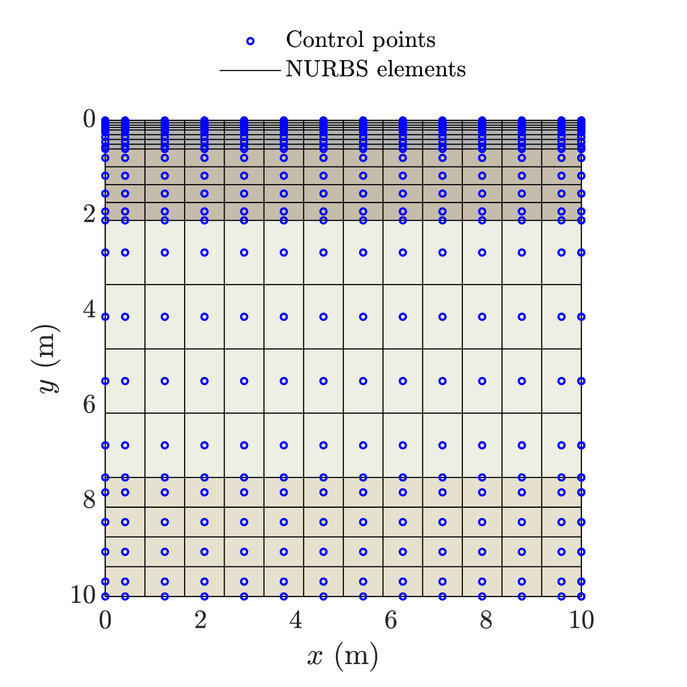

Figure 20: Isogeometric meshes for the two modeling strategies with a soft interlayer, shown for the treated depth \(h=1.5~\mathrm{m}\). (a) Overall layered model; (b) Coupled pavement–subgrade model. Blue circles denote control points and black lines indicate NURBS elements; the light-gray region represents the soft interlayer..
Figs. 21 and 22 show the amplitude of the vertical displacement, denoted by \(V_y\), for different treated depths \(h\). In this parametric study, a transversely concentrated vertical moving load with amplitude \(P=100~\mathrm{kN}\) is applied at \(x_0=3~\mathrm{m}\). The load speed is set to \(c_{\mathrm{load}}=30~\mathrm{m/s}\), and the single-frequency response is evaluated at \(f=10~\mathrm{Hz}\) with \(f_0=0\). This loading configuration is adopted to approximate the effective action range of heavy-vehicle loading in typical service conditions, so that the evaluated sensitivity to \(h\) is of practical relevance. The top of the soft interlayer is located at \[\label{eq:y95int95def} y_{\mathrm{int}} = 0.6 + h,\tag{80}\] where \(0.6~\mathrm{m}\) is the total thickness of the surface and base layers (Table 5).
Fig. 21 presents the free-surface response, i.e., the distribution of \(V_y(x,y=0)\) along the transverse coordinate \(x\). For each treated depth \(h\), results from the overall layered model and the coupled pavement–subgrade model are compared. All curves exhibit a dominant peak near the loading position (\(x\approx x_0\)) and decay rapidly away from it, indicating that the response is mainly governed by a localized near-field zone. With increasing \(h\), both the peak amplitude and the post-peak tail decrease, and the two-model predictions become closer. This behavior indicates that a deeper treated layer reduces the influence of the underlying soft interlayer on the surface motion and weakens the model discrepancy induced by the coupling effect.

Fig. 22 plots the depth-wise variation beneath the load, i.e., \(V_y(x=x_0,y)\) versus depth \(y\). The amplitude decays quickly with depth, and the displacement becomes very small once \(y\) exceeds approximately \(2~\mathrm{m}\). This confirms that, under a vehicle-representative moving load, the effective displacement response is mainly confined to the shallow subgrade. Within this effective range, the influence of \(h\) is most pronounced: the curves separate clearly in the shallow-to-intermediate depths and their relative ordering changes around \(y\approx y_{\mathrm{int}}\), which shifts downward as \(h\) increases. This trend indicates that the impedance contrast across the soft-interlayer interface modifies the wave-field partition and the interference between downward-propagating and reflected components, thereby altering the near-field depth profile.
From a mechanical viewpoint, the interface-sensitive change of \(V_y\) around \(y\approx y_{\mathrm{int}}\) suggests that the interlayer stress response is most pronounced near the soft-interlayer top boundary. Because stresses are governed by spatial derivatives of displacement, a material discontinuity can intensify the local gradients in the vicinity of the interface. Therefore, increasing \(h\) not only reduces the free-surface displacement level, but also shifts the stress-sensitive zone associated with the soft interlayer to a greater depth, weakening its impact on the upper pavement structure.

To further relate the displacement trends to cracking-related indicators, the tensile strain amplitudes at the bottom of the surface layer (\(y=0.2~\mathrm{m}\)) are examined. Fig. 23 shows the distributions of \(\varepsilon_{xx}\) and \(\varepsilon_{zz}\) along the transverse coordinate \(x\) for different treated depths \(h\), with the overall layered model and the coupled model plotted together for each \(h\).
For both components, the response is dominated by a pronounced near-field peak around the loading position (\(x\approx x_0\)), followed by a rapid decay away from the load. Compared with \(\varepsilon_{zz}\), \(\varepsilon_{xx}\) exhibits a more concentrated peak and a stronger sensitivity to \(h\) in the near-field region, indicating that the transverse tensile demand at the surface-layer bottom is more affected by the stiffness change induced by subgrade treatment. A second key feature is observed near the coupling boundary at \(x=4~\mathrm{m}\), where the two modeling strategies start to diverge. In particular, \(\varepsilon_{zz}\) from the overall layered model increases again for \(x\gtrsim 4~\mathrm{m}\), whereas the coupled-model response remains much smaller in the same region. By contrast, \(\varepsilon_{xx}\) shows a sharper, more abrupt change near the coupling boundary and then decays rapidly, indicating a more localized sensitivity to the boundary-induced disturbance. These different patterns suggest that the coupling boundary and the underlying soft interlayer affect the two tensile strain components through different mechanisms: \(\varepsilon_{zz}\) is more influenced by reflected and redistributed wave components that can rebuild the tensile demand away from the load, while \(\varepsilon_{xx}\) is dominated by localized curvature changes and interface-induced strain concentration. Mechanically, these strain patterns imply that subgrade treatment does not only reduce the displacement level, but also redistributes the deformation demand in the surface layer. Increasing \(h\) suppresses the interface-related response near the coupling boundary, while the enhanced near-field concentration of \(\varepsilon_{xx}\) suggests a potential increase in local curvature of the surface layer.

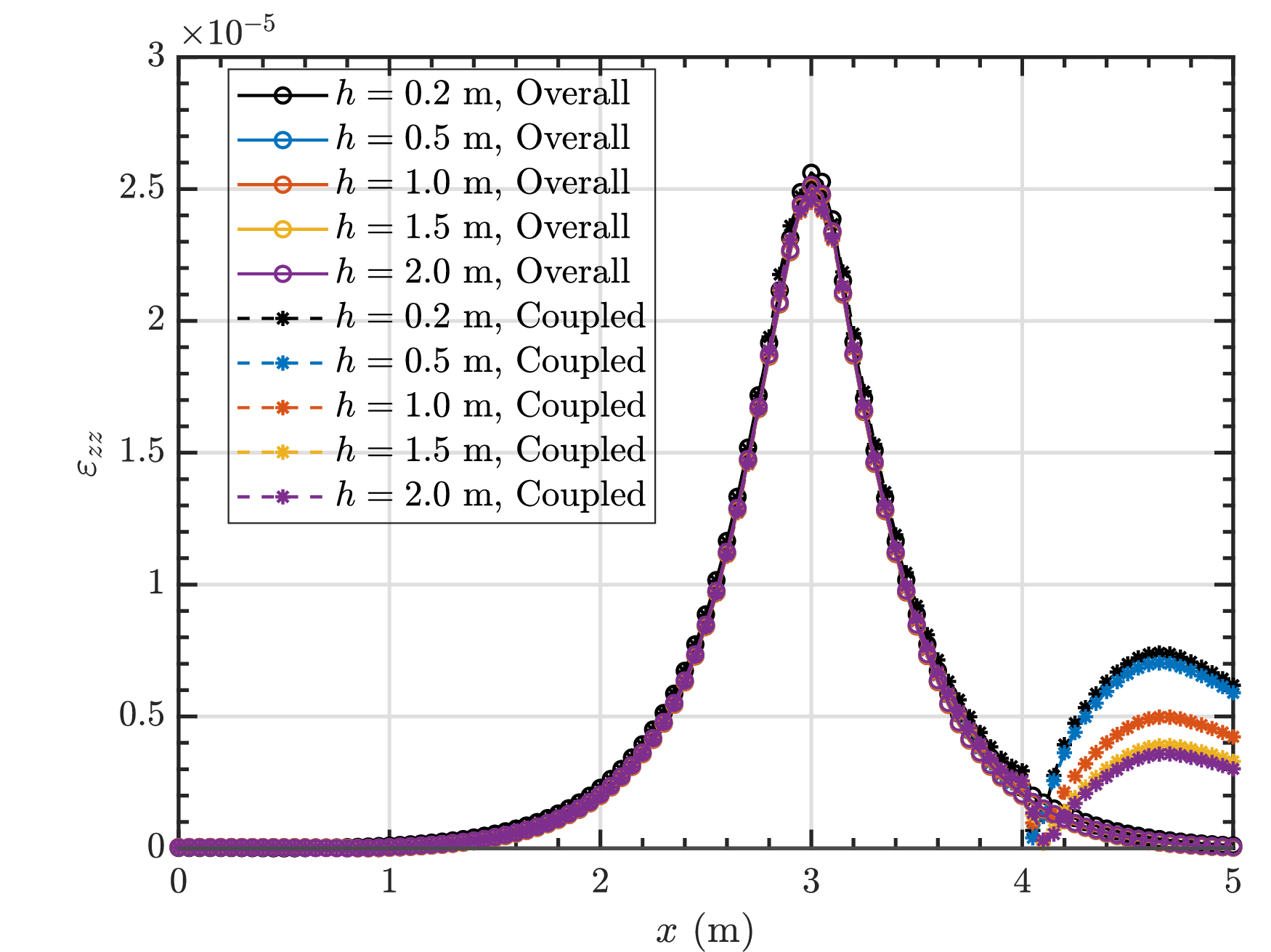
Figure 23: Tensile strain amplitudes at the bottom of the surface layer (\(y=0.2~\mathrm{m}\)) along the transverse coordinate \(x\) under a transversely concentrated moving load (\(P=100~\mathrm{kN}\), \(c_{\mathrm{load}}=30~\mathrm{m/s}\), \(f=10~\mathrm{Hz}\), \(f_0=0\)) applied at \(x_0=3~\mathrm{m}\). Results for different treated depths \(h\) are compared between the overall layered model and the coupled pavement–subgrade model: (a) \(\varepsilon_{xx}\); (b) \(\varepsilon_{zz}\)..
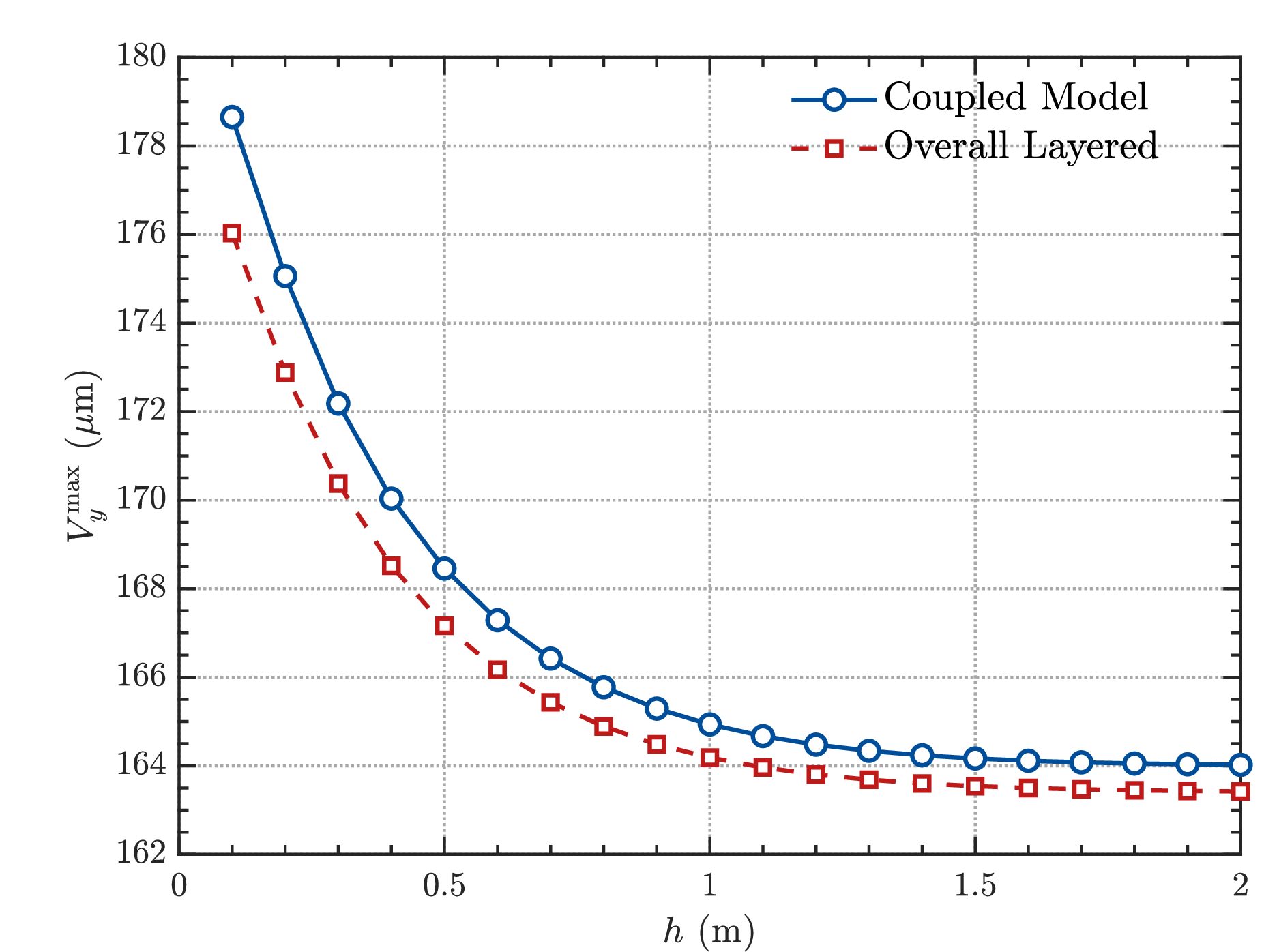
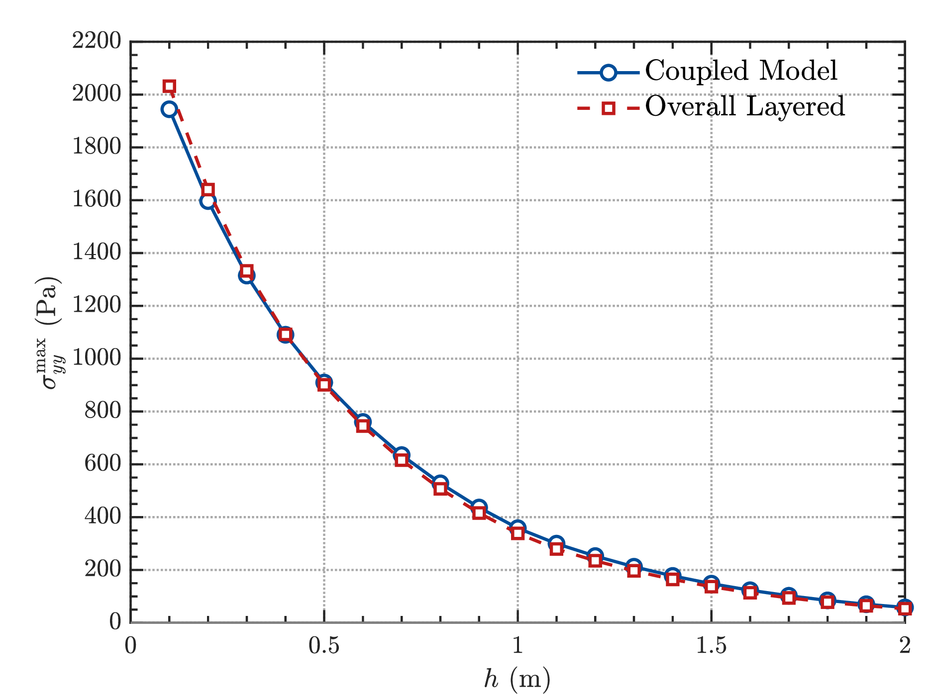
Figure 24: Influence of treated depth \(h\) on rutting-related response indicators. (a) Maximum amplitude of the surface vertical displacement \(V_y^{\max}\); (b) Maximum amplitude of the vertical normal stress at the top of the soft interlayer, \(\sigma_{yy}^{\max}(y=y_{\mathrm{int}})\), where \(y_{\mathrm{int}}=0.6+h\). Results from the coupled model and the overall layered model are compared..
Fig. 24 summarizes two rutting-related indicators as functions of the treated depth \(h\), namely the maximum free-surface vertical displacement amplitude \(V_y^{\max}\) and the maximum vertical normal stress at the top of the soft interlayer, \(\sigma_{yy}^{\max}(y=y_{\mathrm{int}})\) (in Pa). Both indicators decrease monotonically as \(h\) increases, and the reduction is most pronounced for shallow treatment depths. When \(h\) exceeds approximately \(1.2\)–\(1.5~\mathrm{m}\), the curves gradually level off, indicating diminishing marginal benefit from further increasing the treated depth. In addition, the coupled model predicts consistently larger \(V_y^{\max}\) than the overall layered model, especially for small \(h\), whereas the two models give nearly identical predictions for \(\sigma_{yy}^{\max}(y=y_{\mathrm{int}})\) over the full range of \(h\).
Together with the tensile-strain results at the surface-layer bottom, these trends show that the treated depth \(h\) affects several response measures simultaneously within the present linear frequency-domain model. A larger \(h\) reduces the surface displacement and the compressive stress transmitted to the soft interlayer, while also changing the strain concentration pattern in the surface layer. The displacement, stress, and tensile-strain quantities should therefore be interpreted as response indicators rather than as direct rutting or cracking predictions. For the present configuration, increasing \(h\) up to about \(1.2\)–\(1.5~\mathrm{m}\) provides substantial reductions in both \(V_y^{\max}\) and \(\sigma_{yy}^{\max}(y=y_{\mathrm{int}})\), while further deepening yields limited additional improvement. For the present parameters, the response reduction becomes progressively smaller beyond this treatment-depth range, indicating diminishing marginal benefit within the linear dynamic model considered here.
4.3 Speed-dependent responses of ballastless track models under moving line loads: embankment versus cutting↩︎
This example assesses the applicability of the proposed NBIEM to representative ballastless-track cross-sections involving multiple material regions, geometric transitions, and localized wave-field gradients. In contrast to the preceding verification examples, the focus here is not only on the response induced by different moving-load speeds, but also on the ability of the proposed NBIEM discretization to represent practical track-subgrade configurations through a multi-patch layout with compatible patch-wise refinement.
Two typical ballastless-track configurations are considered, as illustrated in Fig. 25: an embankment-type section and a cutting-type section. The model includes all structural components except the rails and is partitioned into four material regions: the track slab, the subgrade surface layer, the subgrade bottom layer, and the underlying embankment. The rails are omitted, and the excitation is represented as moving line loads applied to the track slab, allowing the comparison to focus on the influence of the ground configuration and load speed on the 2.5D wave field. The material properties are summarized in Table 6.


Figure 25: Schematic of the high-speed railway ballastless track cross-sections considered in this study: (a) Cutting section; (b) Embankment section. The model includes the track slab, subgrade surface layer, subgrade bottom layer, and the underlying foundation/ground (rails are not modeled)..
| Material region | \(E\) (GPa) | \(\rho\) (kg/m\(^{3}\)) | \(\nu\) (-) | \(\zeta\) (-) |
|---|---|---|---|---|
| Track slab | 32.5 | 2500 | 0.20 | 0.05 |
| Subgrade surface layer | 0.12 | 2200 | 0.30 | 0.05 |
| Subgrade bottom layer | 0.07 | 1900 | 0.30 | 0.05 |
| Underlying embankment/ground | 0.05 | 1400 | 0.35 | 0.05 |
To represent the cutting- and embankment-type ballastless-track subgrades with sufficient geometric fidelity, the domain is constructed using a multi-patch isogeometric discretization. This strategy enables an accurate partition of the model into subregions with different materials and geometric features, while maintaining an analysis-suitable NURBS parameterization.
The main technical challenge lies in the patch construction and refinement. The geometry includes sharp changes in the surface profile and a sloped transition zone, which require careful patch layout to avoid excessive element distortion. Moreover, local \(h\)-refinement must be performed in a compatible manner across patch interfaces. This demands consistent knot insertion and interface matching so that field continuity and numerical stability are preserved when control points are densified in selected regions. Fig. 26 illustrates the IGA meshes for the two configurations, together with the corresponding locally refined discretizations.


Figure 26: Multi-patch isogeometric meshes for the ballastless-track subgrade models. (a) and (b) show the baseline discretizations for the cutting- and embankment-type configurations, respectively. (c) and (d) show the corresponding locally \(h\)-refined meshes. Blue markers denote control points and black lines denote NURBS elements..
In this example, two rail lines are located at \(x=1.75\) and \(x=3.25~\mathrm{m}\), where moving line loads of amplitude \(75~\mathrm{kN}\) are applied. For each train speed, a single analysis frequency is used according to \(f=c_{\mathrm{load}}/1.5\), where \(1.5~\mathrm{m}\) is the representative sleeper spacing; thus \(c=180\), \(270\), and \(360~\mathrm{km/h}\) correspond to \(f=33.3\), \(50.0\), and \(66.7~\mathrm{Hz}\), respectively, with \(f_0=0\). As a result, the transverse distributions of \(V_y(x)\) in Fig. 27 exhibit a characteristic two-peak pattern at shallow depths, reflecting the superposition of the two rail excitations. With increasing depth, the profiles become broader and smoother, indicating progressive load spreading and wave-field redistribution in the layered subgrade.
A key observation is that the influence of the train speed depends strongly on depth. At the slab bottom (\(y=0.2~\mathrm{m}\), Fig. 27a), the curves for different speeds are close to each other, and the difference between the cutting and embankment configurations is negligible. This suggests that the response at this shallow level is mainly governed by the stiffness and load-spreading capacity of the upper track structure, which tends to attenuate the sensitivity to speed. As the depth increases into the subgrade (\(y=0.6\) and \(1.0~\mathrm{m}\), Fig. 27b–c), the speed effect becomes more visible, while the cutting–embankment discrepancy remains minor throughout. The profiles still retain a clear two-peak shape, implying that the transverse response at these depths is largely controlled by the geometric positions of the rails and the layered transmission of the near-field wave components.
At the deepest interface (\(y=2.9~\mathrm{m}\), i.e., the bottom of the subgrade bottom layer and the top of the underlying embankment/ground, Fig. 27d), the response becomes distinctly speed-dominated. For the low-speed cases (\(c=180\) and \(270~\mathrm{km/h}\)), the magnitude has already decayed to an almost negligible level. In contrast, the high-speed case (\(c=360~\mathrm{km/h}\)) exhibits an order-of-magnitude jump in amplitude, accompanied by a clear change in spatial pattern: the shallow two-peak, rail-localized response transitions into a smoother, wide-hump distribution. This behavior indicates that, under the selected high-speed excitation, a larger portion of the wave field reaches the deeper layers and modifies the response around the subgrade-bottom interface. The observed amplification is consistent with a reduced separation between the moving-load speed and the characteristic wave speeds of the layered ground, although a full critical-speed assessment would require a separate dispersion or velocity-ratio analysis. Consequently, the subgrade-bottom interface should be included when assessing deeper vibration and stress-related responses under high-speed operation, even when the surface-structure responses appear only weakly speed-dependent.


Figure 27: Vertical displacement amplitude \(V_y\) along the \(x\)-direction at four representative depths for the cutting- and embankment-type ballastless-track subgrades under moving-load speeds \(c=180\), \(270\), and \(360~\mathrm{km/h}\). (a) Slab bottom, \(y=0.2~\mathrm{m}\); (b) Bottom of the subgrade surface layer, \(y=0.6~\mathrm{m}\); (c) Mid-depth of the subgrade bottom layer, \(y=1.0~\mathrm{m}\); (d) Bottom of the subgrade bottom layer (top of the underlying embankment/ground), \(y=2.9~\mathrm{m}\)..
Fig. 28 shows the depth-wise profile of the vertical displacement amplitude \(V_y\) at \(x=2.5~\mathrm{m}\), i.e., the mid-point between the two rail load lines (\(x=1.75\) and \(3.25~\mathrm{m}\)). A pronounced near-surface response is observed even though no load is applied directly at \(x=2.5~\mathrm{m}\), which indicates a slab bending/warping effect: the two rail excitations activate a flexural deformation mode of the concrete track slab, leading to a noticeable mid-span vertical motion.
The speed effect is clear. As the speed increases from \(180\) to \(360~\mathrm{km/h}\), the \(V_y\) amplitude increases and its decay with depth becomes slower, indicating enhanced dynamic energy transmission into the subgrade under high-speed excitation. For all speeds, the response attenuates rapidly and becomes very small beyond approximately \(y\approx 2~\mathrm{m}\), suggesting that the deformation demand is mainly concentrated within the upper \(1\)–\(2~\mathrm{m}\) of the foundation in this case. The cutting and embankment curves remain very close over the entire depth range, implying that the depth-wise response at this mid-point is primarily speed-dominated for this metric.


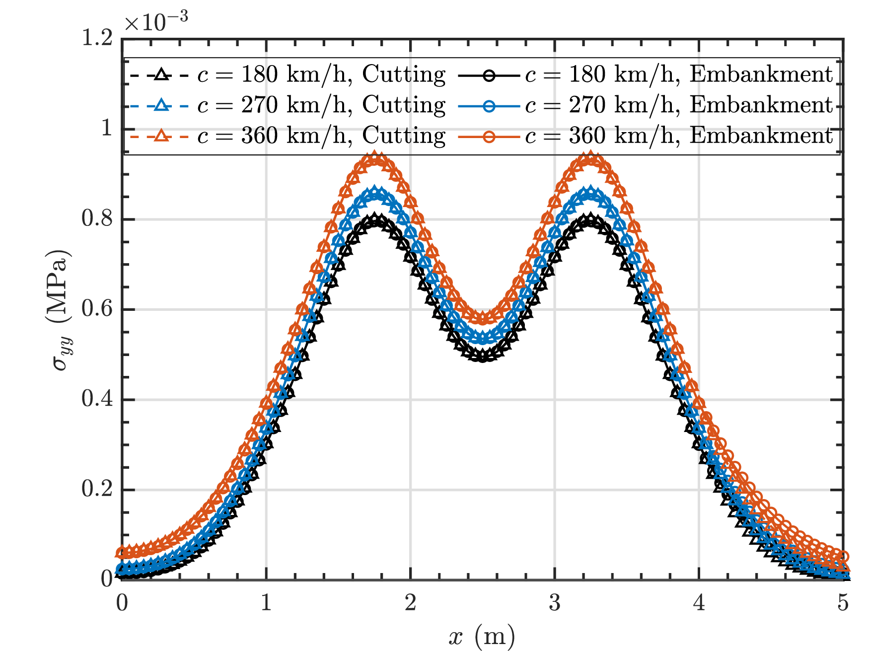

Figure 29: Distributions of the normal stress components at depth \(y=1~\mathrm{m}\) along the transverse coordinate \(x\) for the cutting and embankment track sections under different train speeds (\(c=180\), \(270\), and \(360~\mathrm{km/h}\)).. a — \(\sigma_{xx}\), b — \(\sigma_{yy}\), c — \(\sigma_{zz}\)
Fig. 29 compares the three normal-stress components at \(y=1~\mathrm{m}\) as functions of the transverse coordinate \(x\). All curves exhibit a clear two-peak pattern with a trough in between, consistent with the dual-rail excitation: the two maxima are aligned with the rail load lines, whereas the stress level reduces in the mid-span region. As the train speed increases from \(180\) to \(360~\mathrm{km/h}\), both peak and trough values are amplified while the peak locations remain essentially unchanged, indicating that the speed effect mainly scales the response amplitude at this depth rather than altering the spatial footprint. The differences between the cutting and embankment configurations are minor for all three components, suggesting that the response at \(y=1~\mathrm{m}\) is predominantly speed-controlled under the present layering. In terms of magnitude, \(\sigma_{yy}\) is the dominant component, followed by \(\sigma_{zz}\), whereas \(\sigma_{xx}\) is the smallest. Moreover, \(\sigma_{xx}\) shows a flatter crest and smoother transitions around the two peaks than \(\sigma_{yy}\) and \(\sigma_{zz}\), implying weaker localization due to transverse confinement and redistribution in the layered system.
To complement these line profiles, contour maps of the displacement components \((U,V,W)\) and the normal stresses \((\sigma_{xx},\sigma_{yy},\sigma_{zz})\) are presented in Figs. 30 and 31 for the representative case \(c=270~\mathrm{km/h}\), corresponding to \(f=50~\mathrm{Hz}\) and \(f_0=0\). The plotted fields correspond to the real part of the complex frequency-domain solution at the selected analysis frequency, i.e., \(\Re{\tilde{U}}\), \(\Re{\tilde{V}}\), \(\Re{\tilde{W}}\), and \(\Re{\tilde{\sigma}_{ii}}\). For a harmonic response, the physical field can be written as \(\Re{\tilde{q}(\omega)\exp(\mathrm{i}\omega t)}\); therefore, \(\Re{\tilde{q}}\) represents the in-phase component (the \(t=0\) snapshot up to a phase reference). This visualization provides a consistent view of the spatial redistribution with depth and highlights geometry-related effects near interfaces and slope transitions, while the amplitude information is reported through the line profiles and peak-amplitude comparisons.
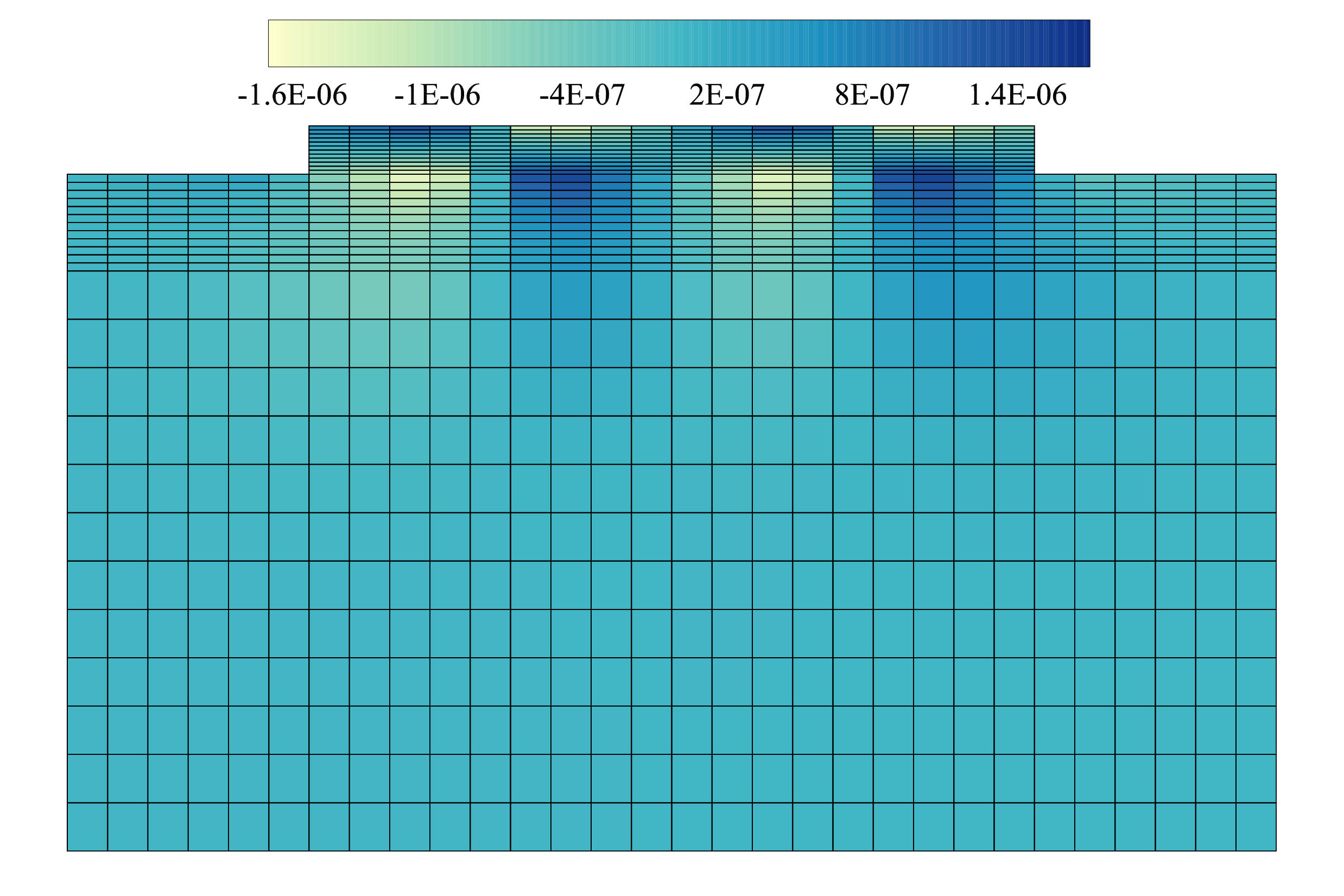
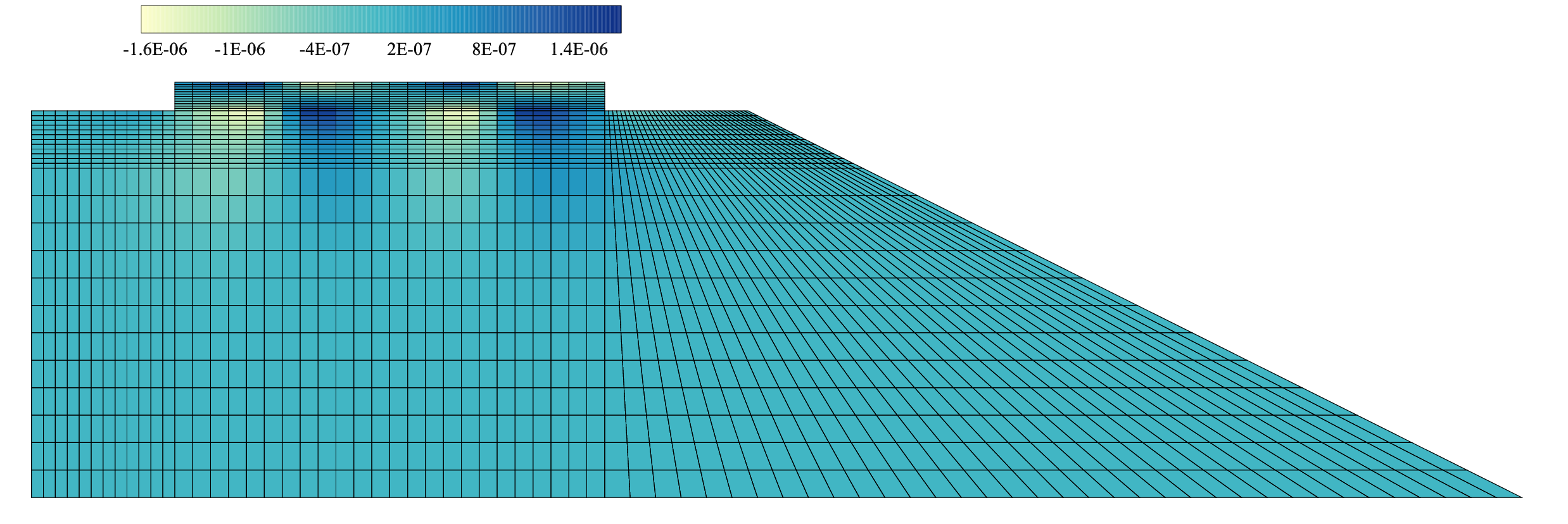

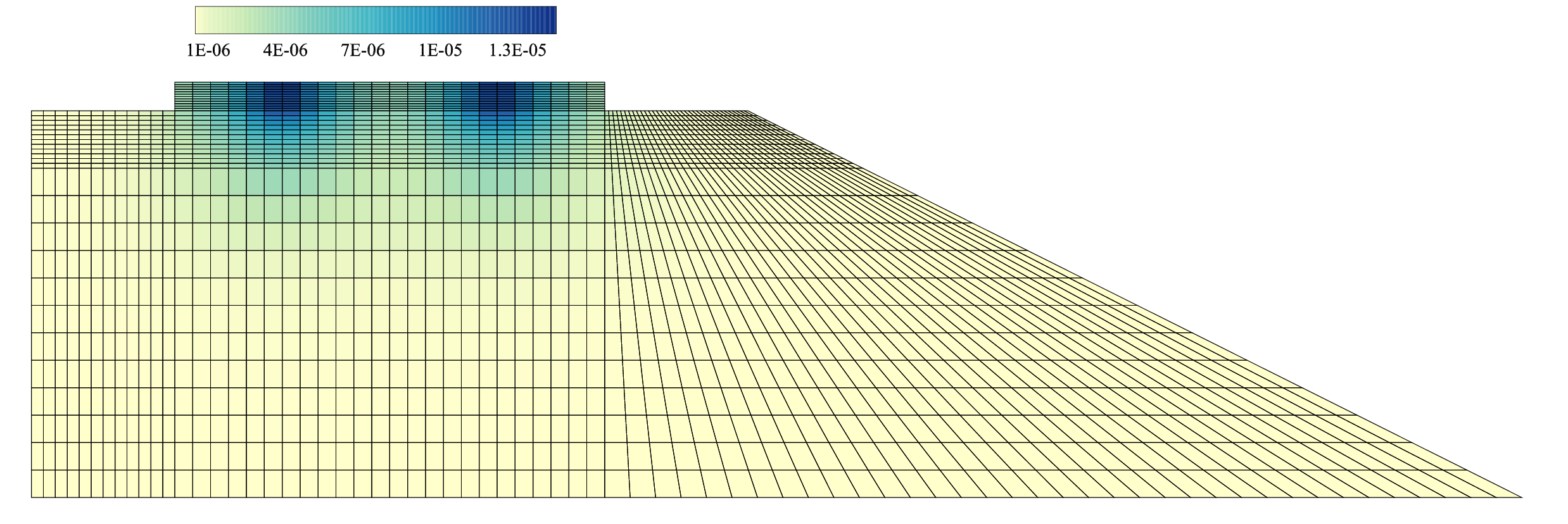

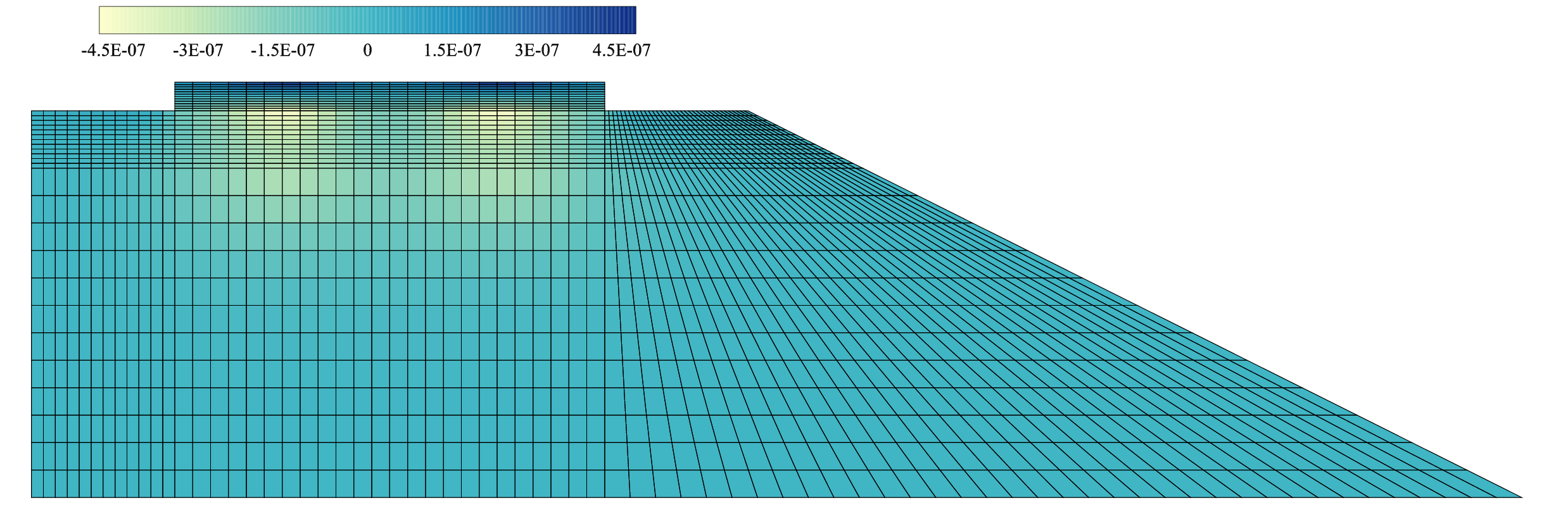
Figure 30: Real-part contour plots of the displacement responses \((U_y,V_y,W_y)\) induced by a \(y\)-directed moving line load for the cutting (left column) and embankment (right column) configurations at \(c=270~\mathrm{km/h}\), \(f=50~\mathrm{Hz}\), and \(f_0=0\)..
The contour plots further confirm that the displacement field is primarily localized in the near-field region beneath the two rail loads, with a clear attenuation trend into the subgrade. Although the cutting and embankment cases exhibit highly consistent overall patterns, subtle geometry-related differences can be observed near the slope transition and layer interfaces, where the wave paths are locally perturbed and the gradients become more concentrated. These full-field visualizations complement the one-dimensional profiles by illustrating how the speed-amplified response is redistributed spatially and where potential interface-sensitive regions may occur.


Figure 31: Real-part contour plots of the normal stresses \((\sigma_{xx},\sigma_{yy},\sigma_{zz})\) induced by the \(y\)-directed moving line loads for the cutting (left column) and embankment (right column) trackbed configurations at \(c=270~\mathrm{km/h}\), \(f=50~\mathrm{Hz}\), and \(f_0=0\). Stress values are reported in Pa..
The stress contours provide a two-dimensional view of how the load-induced response redistributes with depth and across geometric transitions. In all cases, \(\sigma_{yy}\) exhibits the most pronounced concentration beneath the two rail lines and is the dominant compressive component transmitted into the subgrade, whereas \(\sigma_{zz}\) remains appreciable and follows a similar two-lobe footprint, and \(\sigma_{xx}\) is comparatively smoother due to transverse constraint and redistribution. Consistent with the one-dimensional comparisons, the embankment and cutting configurations show only minor differences in the near-track region, while geometry-related effects, when present, become more visible around the slope-transition zone where the stress field spreads and attenuates along the ground surface.
4.4 Cover-depth-dependent wave attenuation in layered ground containing a buried tunnel↩︎
To quantify the influence of tunnel burial depth on load-induced wave attenuation, this example considers a circular metro tunnel embedded in layered ground and subjected to a vertical surface moving load applied directly above the tunnel axis (at \(x=8~\mathrm{m}\) in the cross-sectional coordinate system). The tunnel configuration is sampled from Zhengzhou Metro Line 1. As illustrated in Fig. 32, the underground structure is represented by a reinforced-concrete segmental lining together with the surrounding grouting layer outside the lining, while the geological profile is represented as a two-layer soil deposit consisting of silty clay over silt. The single-frequency response is evaluated for a nominal surface load amplitude \(P=150~\mathrm{kN}\), \(f=10~\mathrm{Hz}\), \(f_0=0\), \(c_{\mathrm{load}}=35~\mathrm{m/s}\), and \(k=(\omega-\omega_0)/c_{\mathrm{load}}\). In this setting, the burial depth controls the propagation and attenuation of vibration energy from the ground surface to the tunnel level. The loading and exterior-boundary construction are kept fixed to provide a consistent comparison of the cover-depth trends within the selected computational configuration.
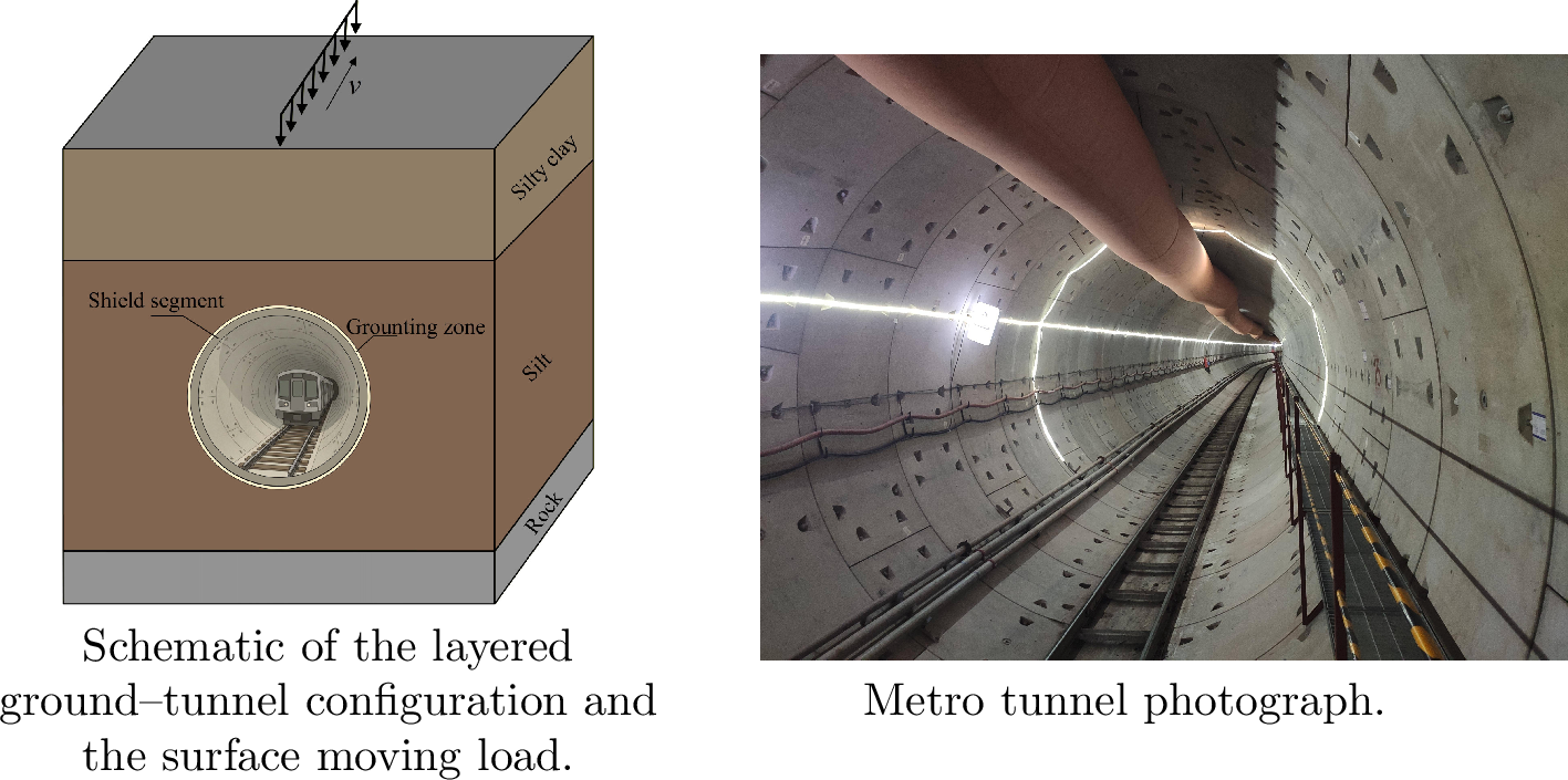
Fig. 32 summarizes the ground–tunnel configuration adopted for the burial-depth study. The bounded near-field domain is 15 m wide in the transverse direction and 25 m deep, and the tunnel axis is located 8 m from the left boundary so that the surface moving load can be applied directly above the tunnel centerline at the same transverse location. This depth keeps the grouting-zone invert inside the bounded near field before the lower infinite boundary is attached; in the deepest case, the grouting-zone invert is located at \(h_e+D_{\mathrm{grout}}=19.6~\mathrm{m}\), leaving a 5.4 m clearance to the lower near-field boundary. The ground is represented as a two-layer profile representative of Zhengzhou Metro Line 1, consisting of an upper silty-clay stratum with a fixed thickness of 6.8 m overlying a silt stratum, and the tunnel is embedded in the silt layer. The burial depth is characterized by the crown cover depth, defined as the vertical distance from the ground surface to the tunnel crown. Four burial-depth cases are considered, with crown cover depths of 8 m, 10 m, 12 m, and 14 m, which form the basis of the subsequent comparisons. The underground structure is modeled using a reinforced concrete segmental lining surrounded by a grouting zone. The lining inner diameter is taken as 5.4 m, the lining outer diameter as 5.5 m, and the grouting-zone diameter is \(D_{\mathrm{grout}}=5.6~\mathrm{m}\).
The corresponding IGA discretization is shown in Fig. 33, where a multi-patch construction is used to represent the circular interfaces accurately and to maintain a conforming connection between the lining, the grouting zone, and the surrounding ground. Local h-refinement is introduced in the near-field region, particularly along the surface load path and around the tunnel boundary, to resolve the strong displacement gradients and stress concentration induced by the moving excitation. Away from the tunnel, a coarser discretization is adopted to control the total degrees of freedom. The material parameters are summarized in Table 7, covering the silty-clay and silt strata, the shield segments, and the grouting region. Unless otherwise stated, the same viscoelastic damping setting as in the previous examples is used so that the parametric comparisons remain consistent across all cases.
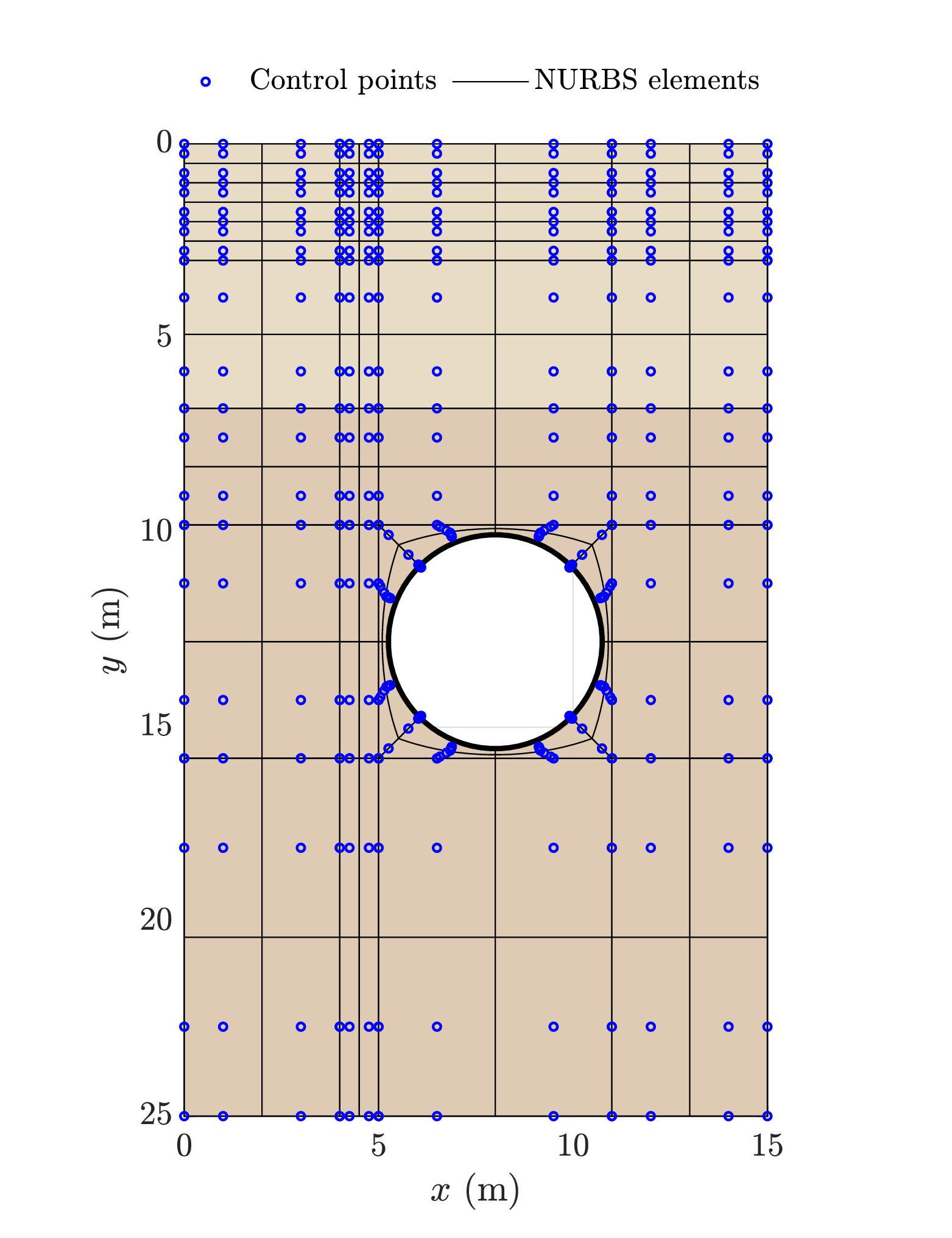

Figure 33: IGA discretizations for the tunnel example. Blue dots denote control points and black lines denote NURBS elements. (a) Baseline multi-patch mesh used to represent the circular tunnel boundary and the surrounding ground. (b) Locally \(h\)-refined mesh with increased resolution around the tunnel lining and in the near-surface region along the load path to capture strong displacement/stress gradients..
| Layer/Region | \(E\) (MPa) | \(\rho\) (kg/m\(^{3}\)) | \(\nu\) (-) | \(\zeta\) (-) |
|---|---|---|---|---|
| Silty clay | 23 | 2143 | 0.30 | 0.05 |
| Silt | 17 | 1959 | 0.30 | 0.05 |
| Shield segment | 30000 | 2551 | 0.20 | 0.05 |
| Grouting zone | 500 | 2245 | 0.30 | 0.05 |
Here \(x\) denotes the transverse coordinate in the cross-section, and the tunnel axis is located at \(x=8~\mathrm{m}\) so that the surface line load is applied directly above the tunnel centerline. The crown cover depth is denoted by \(h_e\), defined as the vertical distance from the ground surface to the tunnel crown. To examine the attenuation of the surface-load-induced response in the soil above the tunnel, response profiles are extracted at several elevations above the crown, quantified by \(\Delta y\). Specifically, a profile with a given \(\Delta y\) corresponds to the horizontal line located at the depth \(y=h_e-\Delta y\) in the adopted coordinate system (positive \(y\) downward).
Figs. 34 and 35 show the transverse distributions of \(U_y\) and \(V_y\) along \(x\) at four elevations above the tunnel crown, \(\Delta y=2\), \(3\), \(4\), and \(5~\mathrm{m}\), for different crown cover depths \(h_e=8\), \(10\), \(12\), and \(14~\mathrm{m}\). For all cases, the responses are concentrated around the loading position (\(x=8~\mathrm{m}\)), and the amplitude decays rapidly away from the load, indicating a localized near-field influence in the transverse direction. As \(h_e\) increases, both \(U_y\) and \(V_y\) decrease systematically at all considered \(\Delta y\) levels, and the curves become progressively closer to the zero baseline, which demonstrates that a larger cover depth promotes stronger attenuation before the vibration field reaches the region above the tunnel crown. The dependence on \(\Delta y\) is also clear: larger \(\Delta y\) values correspond to shallower monitoring lines closer to the surface load and therefore produce larger displacement amplitudes and broader influence zones. Monitoring lines closer to the tunnel crown, corresponding to smaller \(\Delta y\), exhibit weaker responses because of the longer propagation distance from the surface excitation.
From an engineering perspective, these trends indicate that increasing the crown cover depth reduces both the intensity and the spatial extent of the displacement disturbance reaching the crown-adjacent soil region. For the deeper configurations (e.g., \(h_e=12\)–\(14~\mathrm{m}\)), the responses extracted above the crown become markedly smaller than those for the shallow case (\(h_e=8~\mathrm{m}\)), and the incremental reduction from \(h_e=12\) to \(14~\mathrm{m}\) appears more limited, suggesting a tendency toward convergence in the attenuation effectiveness. Under the selected material, loading, and geometric conditions, these trends indicate that increasing cover depth can reduce the vibration disturbance transmitted to the ground above the tunnel, with a smaller incremental change for the deeper cases.


Figs. 36 and 37 report the distributions of the normal stresses \(\sigma_{xx}\) and \(\sigma_{yy}\) along the transverse coordinate \(x\) at a set of monitoring lines located \(\Delta y=2\)–\(5~\mathrm{m}\) above the tunnel crown, for four cover depths \(h_e=8\), \(10\), \(12\), and \(14~\mathrm{m}\). Here \(\Delta y\) denotes the vertical distance from the tunnel crown to the monitoring line, so a larger \(\Delta y\) corresponds to a shallower observation line closer to the ground surface. For each \(h_e\), both stress components exhibit a single dominant peak centered at \(x\approx 8~\mathrm{m}\), which coincides with the surface load position directly above the tunnel axis. The peak location remains essentially unchanged across all \(h_e\) and \(\Delta y\), indicating that, within the present parameter range, the geometry primarily modulates the response magnitude and the lateral spreading rather than shifting the stress concentration zone in plan.
The influence of \(\Delta y\) is systematic and can be read directly from the curve ordering. For all \(h_e\), the stress amplitude increases monotonically with \(\Delta y\), with the \(\Delta y=5~\mathrm{m}\) curve consistently being the largest and the \(\Delta y=2~\mathrm{m}\) curve the smallest. In addition to the peak height, the peak width also expands as \(\Delta y\) increases, and the post-peak tails decay more slowly, implying a broader lateral influence range at shallower depths. This behavior is consistent with depth-dependent attenuation and load-spreading in layered media. At smaller \(\Delta y\) the observation line is closer to the tunnel and deeper in the soil deposit, whereas at larger \(\Delta y\) the monitoring line approaches the near-surface region where the stress path is shorter and the wave field has undergone less geometric attenuation, leading to higher stress levels and a wider footprint.
The cover depth \(h_e\) produces an even stronger effect in terms of amplitude scaling. From \(h_e=8~\mathrm{m}\) to \(10~\mathrm{m}\) the peak level decreases markedly, and further increases to \(h_e=12\) and \(14~\mathrm{m}\) drive the stress curves into progressively smaller orders of magnitude, as reflected by the changing axis scales in the subpanels. Meanwhile, the overall curve shapes remain similar, suggesting that increasing \(h_e\) mainly enhances the attenuation between the surface excitation and the crown-adjacent region, rather than altering the fundamental load-transfer pattern. Practically, this indicates a rapid reduction of the computed stress response in the soil mass above the tunnel once the cover depth becomes sufficiently large, after which the marginal benefit of further burial becomes limited.
Comparing the two stress components, \(\sigma_{yy}\) is consistently larger than \(\sigma_{xx}\) for all \(h_e\) and \(\Delta y\), and its peak is sharper with steeper flanks. In contrast, \(\sigma_{xx}\) shows a flatter crest and smoother transitions. This contrast is physically expected. \(\sigma_{yy}\) is more directly aligned with the dominant vertical transmission path of the surface load and therefore retains stronger localization. \(\sigma_{xx}\) is governed by transverse confinement and lateral redistribution, which act as a spatial smoothing mechanism and weaken the peak effect. The combined observation implies that the crown-above soil region is primarily driven by vertical compression demand, while transverse normal stress plays a secondary role and is less sensitive to local concentration.
Under the present ground profile and structural configuration, the dynamic stress disturbance above the tunnel becomes substantially weaker once \(h_e\) reaches about \(12~\mathrm{m}\), because both \(\sigma_{xx}\) and \(\sigma_{yy}\) at \(\Delta y=2\)–\(5~\mathrm{m}\) above the crown have already dropped to very small levels and the curves become less distinguishable. This trend should be interpreted as a model-based indication of diminishing cover-depth sensitivity for the selected stratified ground rather than as a general design threshold.

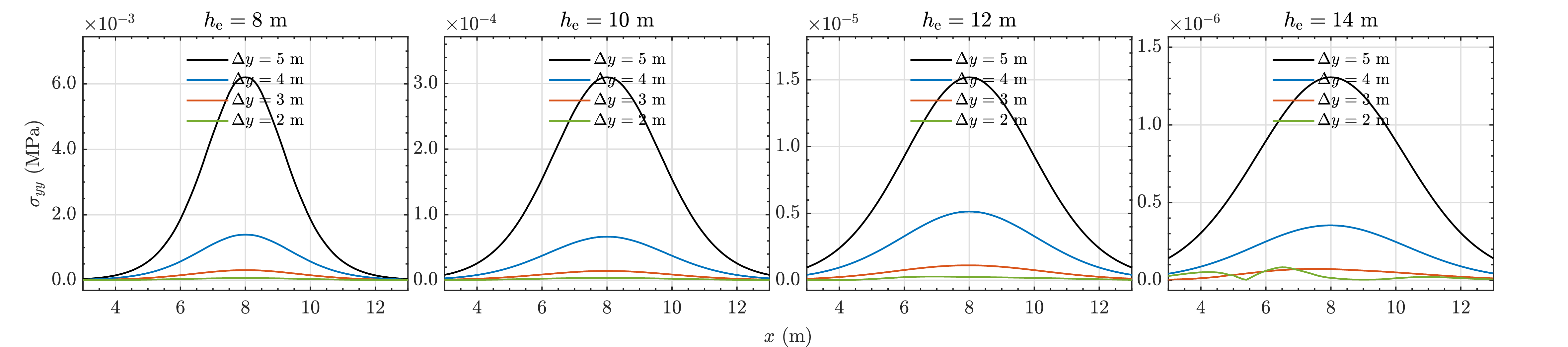
5 sec:Discussion↩︎
The numerical results position NBIEM as an efficient boundary-attached exterior formulation for repeated frequency-domain analyses of wave propagation in semi-infinite ground. Under matched physical cross-sectional partitions, the different approximation spaces lead to different global numbers of degrees of freedom, and these differences are retained as part of the performance assessment. From the intermediate-frequency cases onward, the proposed formulation provides a favorable balance between displacement and phase accuracy and computational cost. Relative to IGA/SBIGA, the semi-infinite exterior is represented directly through far-field stiffness and mass contributions assembled on the shared NURBS trace, without constructing a separate scaled-boundary dynamic-stiffness system.
The formulation also provides a distinct alternative to other exterior treatments used in geotechnical wave analysis. PML formulations typically represent the exterior through an absorbing layer and coordinate stretching, whereas FE–BE formulations describe radiation through problem-specific fundamental solutions and boundary-integral evaluation. In NBIEM, the exterior response is represented through outgoing or evanescent radial functions attached to the artificial boundary, and the associated radial moments are evaluated in closed form. The resulting construction preserves the geometric representation and approximation continuity of the bounded IGA domain while maintaining a compact exterior discretization.
For engineering applications, the all-S realization provides a consistent and explicitly defined default setting. Its decay parameter is determined from the exterior material properties and the declared geometric scale of each boundary segment, without frequency-by-frequency optimization or access to an analytical reference response. The indicators \(I_{\beta}\) and \(I_D\) complement this setting by quantifying the response sensitivity to the radial decay parameter and to the artificial-boundary location. The calibrated mixed-wave realization further demonstrates, in the benchmark setting, how additional wave information can improve low-frequency agreement.
The engineering examples focus on controlled single-frequency configurations so that the influence of material layering, structural geometry, moving-load speed, treatment depth, and tunnel cover depth can be examined within clearly defined configurations. The multi-patch construction accommodates material interfaces and curved internal boundaries while retaining a common NURBS-based representation. These examples demonstrate how the proposed exterior treatment can be integrated into layered-ground, track–subgrade, and buried-structure models without changing the basic near–far-field coupling procedure.
The present framework also provides several directions for further development. Richer radial approximation spaces may extend the frequency range of the exterior representation, while nonlinear or coupled constitutive models, interface interaction, and more detailed vehicle–track loading descriptions would broaden the range of geotechnical applications. Further comparisons with field measurements, established benchmark datasets, and large-scale three-dimensional simulations would provide additional physical assessment of the method.
6 sec:Conclusions↩︎
This study developed a three-component 2.5D formulation that couples a bounded isogeometric near field to NURBS-trace infinite elements for moving-load wave propagation and dynamic soil–structure interaction in semi-infinite geotechnical media. The bounded isogeometric domain and the semi-infinite exterior share the same discrete NURBS trace and boundary control-point unknowns, providing a direct and geometrically consistent near–far-field coupling. For the selected outgoing or evanescent exponential radial functions, the radial moments entering the far-field stiffness and mass matrices are evaluated in closed form, without introducing a finite radial truncation or radial numerical quadrature.
Analytical half-space benchmarks confirm that the formulation reproduces displacement and stress responses of a viscoelastic half-space over different moving-load speed regimes. The numerical studies characterize the working behavior of the exterior approximation over different frequencies, radial settings, and artificial-boundary configurations. The sensitivity indicators \(I_{\beta}\) and \(I_D\) provide practical diagnostics for assessing the selected exterior setting, while the method comparisons demonstrate the computational potential of the formulation for repeated frequency-domain analyses.
The engineering examples further demonstrate the applicability of the method to layered ground, track–subgrade systems, and buried structures involving material interfaces, compatible multi-patch discretizations, and curved boundaries. Overall, the results identify NBIEM as an efficient and geometry-consistent computational framework for 2.5D frequency-domain analyses of wave propagation and dynamic soil–structure interaction in semi-infinite ground.
Acknowledgements↩︎
Bei Zhang acknowledges financial support from the National Natural Science Foundation of China (Grant No. 52478477). Yanhui Zhong acknowledges financial support from the National Natural Science Foundation of China (Grant No. 52578540) and the Henan Provincial Natural Science Foundation (Grant No. 252600421827). Quansheng Zang acknowledges financial support from the China Postdoctoral Science Foundation (Grant No. 2024M752937), the Henan Provincial Science and Technology Research Project (Grant No. 262102221015), and the Key Research Projects of Higher Education Institutions in Henan Province (Grant No. 25A560006). Hao Hong acknowledges financial support from the Zhengzhou University Young Student Basic Research Projects (PhD Students) (Grant No. ZDBJ2026065).