A JoLT for the KV Cache:
Near-Lossless KV Cache Compression via Joint Tucker and JL-Residual Allocation for LLMs
July 14, 2026
Abstract
The key-value (KV) cache has become the dominant memory cost of transformer inference. It grows with batch size, context length, and depth, and at long context it, rather than the model weights, sets the ceiling on throughput. Two families of methods reduce it. Low-rank methods factor two-dimensional slices of the cache, either per-head matrices or cross-layer feature blocks, and quantization methods lower the bit-width of every entry. Neither family exploits the fact that the cache at a layer is naturally a third-order tensor whose three axes, the heads, the tokens, and the features, carry very different amounts of redundancy. We take this tensor view directly. Our method, JoLT, applies a partial Tucker decomposition that compresses only the token and feature axes while leaving the head and layer axes intact, and then restores the energy that truncation discards with a Johnson-Lindenstrauss (JL) rotated low-bit residual. A single Lagrangian dual allocates the Tucker ranks and the residual bit-widths together, per layer group and separately for keys and values, under one byte budget. The result is a near-lossless \(2\)–\(3\times\) compression: perplexity, GSM8K accuracy, and RULER needle-in-a-haystack retrieval all stay at or within statistical noise of the uncompressed baseline on both a grouped-query-attention model (Mistral-7B-v0.3) and a multi-head-attention model (LLaMA-2-13B). At \(2\times\), JoLT reconstructs the cache to relative Frobenius error \(0.009\) (K) and \(0.006\) (V) on both architectures, roughly an order of magnitude below cross-layer SVD and 4-bit quantization. A randomized-SVD variant, FlashJoLT, delivers a \(5\)–\(13\times\) compression-time speedup at matched quality.
1 Introduction↩︎
Every step of autoregressive transformer inference reuses the key and value projections of all previous tokens, so an implementation caches them at every layer rather than recomputing them [1]. This KV cache grows as \(O(\text{batch} \times T \times L \times n_h \times d_h)\), and once the context is long or the batch is large it, not the model weights, becomes the memory bottleneck and the binding constraint on throughput. Shrinking the cache without hurting model quality is therefore a direct lever on how cheaply a model can serve long contexts, which is the problem we study.
Two families of methods address this bottleneck, and each commits early to a particular view of the cache. Low-rank methods treat the cache as a collection of matrices and factor those matrices: Palu projects the per-head key and value matrices onto low-rank subspaces [2], while xKV factors stacked cross-layer feature blocks [3]. Quantization methods instead keep the full cache but lower the bit-width of every entry [4], [5]. Both families are effective, yet both leave structure on the table. A two-dimensional factorization must commit to one axis of redundancy and ignore the others, and a fixed-bit-width quantizer cannot reach the modest, intermediate compression ratios where quality is still free, because its smallest setting already overshoots them. What is missing is a view of the cache that sees all of its axes at once and spends a shared budget across them.
We take that view by treating the cache at a layer as a third-order tensor \(K_l \in \mathbb{R}^{n_h \times T \times d_h}\) and asking, empirically, which of its axes actually carry compressible structure. The answer is uneven: the head and layer axes are essentially incompressible, while the token and feature axes hold almost all of the redundancy, and within those the values(cache) are consistently harder to compress than the keys. This observation motivates our method, JoLT (Joint Tucker and JL-residual allocation). Rather than compress every axis, JoLT applies a partial Tucker decomposition that truncates only the token and feature axes and leaves the head and layer axes intact, and it then restores the energy that truncation discards with a JL-rotated low-bit residual. Because keys and values have different spectra, a single Lagrangian dual allocates the Tucker ranks and the residual bit-widths jointly, per layer group and separately for keys and values, under one byte budget. The method works because it places the budget exactly where the redundancy is and lets the dual move bits between ranks and residual, and between keys and values, instead of fixing that split in advance.
Our contributions are the following.
A spectral analysis of real KV caches (Section 3) that locates the compressible structure: the head and layer axes are incompressible, the token and feature axes carry the redundancy, and values are \(2\)–\(3\times\) harder than keys. This is what motivates a partial decomposition with separate key and value budgets, rather than a full tensor factorization.
JoLT (Section 4), which couples a partial Tucker backbone with a JL-rotated residual and allocates ranks and residual bits through a single Lagrangian dual per (layer group, K/V). The joint allocation is what turns a lossy backbone into a near-lossless one in a \(2\)–\(3\times\) free zone.
FlashJoLT (Section 5), a randomized-SVD variant with tail-mass accounting that preserves free-zone quality while cutting compression time \(5\)–\(13\times\), which keeps the method practical at the long contexts where the cache matters most.
An empirical study on a GQA and an MHA model (Sections 6–8) that establishes the free zone, surfaces a sharp GQA-versus-MHA split beyond it, and isolates each design choice through ablations.
2 Related Work↩︎
2.0.0.1 Low-rank KV compression.
The closest line of work compresses the cache by exploiting low-rank structure, and existing methods differ mainly in which two-dimensional slice they factor. Palu factorizes the key and value projection weights by SVD and stores a low-rank latent cache that it reconstructs at attention time [2], whereas xKV extracts aligned singular vectors across layers and factors grouped cross-layer keys and values onto a shared low-rank subspace [3]. Both are matrix methods: they commit to one axis of redundancy and never see the cache as a single object across heads, tokens, and features. Our spectral analysis shows why this matters, since the right place to put low-rank structure is the token and feature axes jointly while the head and layer axes stay intact, and since reaching near-lossless fidelity additionally requires a residual term that pure low-rank factorization does not provide. Eviction methods, which drop low-importance tokens rather than compress them, are orthogonal and can be combined with ours [6]–[8].
2.0.0.2 Quantization.
A second family keeps the full cache and lowers the bit-width of each entry. KIVI applies tuning-free asymmetric 2-bit quantization [4], per-token 4-bit quantization is a common strong baseline, and TurboQuant is a near-optimal-distortion vector quantizer [5]. These methods are strong at their native bit-rates, but a fixed-bit-width scheme saturates at a corresponding compression floor; a 4-bit scheme, for instance, cannot reach below roughly \(4\times\). JoLT instead targets intermediate budgets continuously across \(2\)–\(10\times\), which includes the \(2\)–\(3\times\) band that a fixed 4-bit quantizer simply cannot express. We therefore see quantization as complementary rather than as a direct competitor in that band.
2.0.0.3 Tensor decompositions.
JoLT builds on classical multilinear algebra. Tucker [9], [10], CP [11], tensor-train [12], and t-SVD [13] are the standard formats for third-order tensors, and we use a partial Tucker decomposition chosen for the cache’s specific mode structure, paired with a JL residual [14] and, in the fast variant, a randomized SVD [15]. The partial form is not an arbitrary choice: a full multilinear comparison (Appendix 11.2) shows Tucker is the best of these formats at every ratio on both architectures, and that compressing the index-like head and layer axes is what hurts.
3 Spectral Motivation↩︎
Before designing a compressor, we measure where the redundancy in a KV cache actually lives. We unfold the cache of Mistral-7B layer 15 (\(T{=}1024\)) along each of its three axes and take the singular values of each unfolding; the full table is in Appendix 10, and three facts stand out.
First, the head axis is essentially incompressible. The ratio of largest to smallest singular value across heads is only about \(1.5\) for keys and \(1.4\) for values, which means every KV head carries roughly the same energy and none can be dropped cheaply. This is expected for a grouped-query model, where GQA [16] has already merged redundant heads upstream, and it tells us not to spend budget on this axis. Second, the token axis is where most of the opportunity lies, but keys and values behave very differently along it: the key unfolding reaches \(10\%\) error at rank \(228\) of \(1024\), whereas the value unfolding needs rank \(563\). Third, the feature axis is compressible for keys but nearly isotropic for values, with a singular-value ratio of \(27.4\) for keys against only \(2.7\) for values.
These measurements expose a robust asymmetry that drives the rest of the design: values are \(2\)–\(3\times\) harder to compress than keys at every ratio and for every format we tested (Appendices 11.2 and 11.1). The mechanism is the projection geometry. The value projection \(W_V\) spreads energy across feature directions so that the weighted sum preserves content, whereas the key projection \(W_K\) concentrates energy into the few directions that decide the softmax score, leaving the value spectrum flat and the key spectrum sharply decaying. Two design consequences follow directly. Because compressing the head axis is always a loss, and likewise the small, semantically distinct layer axis (Appendix 11.1), we pin both and truncate only the token and feature axes. And because keys and values sit at opposite ends of the compressibility scale, they must receive separate rank and bit budgets rather than a shared one.
4 Method: Joint Tucker and JL Allocation (JoLT)↩︎
JoLT compresses the cache in two stages and decides how hard to push each stage with one optimizer. We first partition the \(L\) layers into \(G\) contiguous groups and, within each group \(g\), treat the keys and the values as separate compression targets \(t \in \{\mathrm{K}, \mathrm{V}\}\). For each pair \((g, t)\) we apply a partial Tucker decomposition that truncates only the token and feature axes, encode the resulting truncation residual with a JL-rotated low-bit code, and let a single Lagrangian dual choose the Tucker ranks and the residual bit-width that meet a global byte budget. The three components below correspond to these stages, and we present each as motivation, design, and the advantage it buys.
4.0.0.1 Partial Tucker backbone.
The role of the backbone is to remove the redundancy the spectral analysis identified, and only that redundancy. For a grouped tensor \(X \in \mathbb{R}^{|g| \cdot n_h \times T \times d_h}\), the partial Tucker approximation \(\tilde{X}(r_T, r_d)\) truncates the token mode to rank \(r_T\) and the feature mode to rank \(r_d\) through their mode-\(k\) singular vectors, using the sequentially truncated higher-order SVD (ST-HOSVD) [17], while keeping identity factors on the head and layer modes. Pinning those two modes is not a heuristic shortcut but the empirically optimal choice: when we instead give a full four-mode allocator freedom over all axes, it drives the head and layer ranks back to their full size on every group and ratio we tested, producing byte-identical output (Appendix 11.2). Decomposing only the token and feature modes is therefore lossless relative to the full search, and it runs \(2.4\)–\(3.0\times\) faster than full HOOI at identical error.
4.0.0.2 JL residual.
A pure low-rank backbone cannot reach near-lossless fidelity on its own, because truncation discards real energy, and on the flat value spectrum that energy is large. The residual recovers it. We take the truncation residual \(R = X - \tilde{X}(r_T, r_d)\), apply a Johnson-Lindenstrauss random rotation, and quantize the rotated residual uniformly at \(b \in \{0, 2, 4, 8\}\) bits per entry, where \(b{=}0\) means no residual is stored [14]; decoding simply inverts the rotation. This residual is the lever that turns a lossy backbone into a near-lossless one at low ratio, and it is especially valuable on the values, whose flat spectrum makes residual bits far more productive than additional rank.
4.0.0.3 Joint Lagrangian allocation.
The two stages compete for the same bytes, so we allocate across them jointly rather than fixing the split in advance. Consider a single (layer group, tensor) cell \((g, t)\), write \(m = |g|\, n_h\) for its merged head-and-layer count, and let \(c\) be the bytes per stored scalar. A choice of token rank \(r_T\), feature rank \(r_d\), and residual width \(b\) then costs \[s_{g,t}(r_T, r_d, b) \;=\; \underbrace{\big( m\, r_T r_d + T r_T + d_h r_d \big)\, c}_{\text{Tucker core and factors}} \;+\; \underbrace{\tfrac{b}{8}\, m\, T\, d_h}_{\text{packed JL residual}} \label{eq:bytes}\tag{1}\] bytes, up to a negligible per-row scale term, and it incurs a reconstruction error we model as \[e_{g,t}(r_T, r_d, b) \;\approx\; \varepsilon^2(b)\,\cdot\,\tau_{g,t}(r_T, r_d) . \label{eq:err}\tag{2}\] Here \(\tau_{g,t}(r_T, r_d)\) is the relative Frobenius mass that the partial Tucker truncation discards at ranks \((r_T, r_d)\), and \(\varepsilon^2(b)\) is the fraction of that discarded mass the JL-rotated \(b\)-bit residual fails to recover, calibrated once on a Gaussian round-trip with \(\varepsilon^2(0){=}1\) and \(\varepsilon^2\) decreasing in \(b\). This factorization is what makes the two stages comparable in one budget: rank buys a smaller truncation tail \(\tau\), while bits buy a smaller residual factor \(\varepsilon^2(b)\), and Equation 2 prices both on the same error scale.
Given a total byte budget \(B\), JoLT minimizes the summed error subject to the summed cost, \[\min_{\{(r_T, r_d, b)_{g,t}\}} \; \sum_{g,t} e_{g,t}(r_T, r_d, b) \quad \text{s.t.} \quad \sum_{g,t} s_{g,t}(r_T, r_d, b) \le B . \label{eq:problem}\tag{3}\] We solve this through its Lagrangian relaxation, \[\mathcal{L}(\lambda) \;=\; \sum_{g,t} \Big[\, e_{g,t}(r_T, r_d, b) + \lambda\, s_{g,t}(r_T, r_d, b) \,\Big], \label{eq:lagrangian}\tag{4}\] which separates across cells. For a fixed multiplier \(\lambda\) each cell is minimized independently over its finite \((r_T, r_d, b)\) grid, and a single bisection on \(\lambda\) drives the total cost to the budget \(B\). This joint solve is the design advantage over per-tensor heuristics: a greedy or rank-only allocator cannot move bits between keys and values, or between ranks and residual, whereas the dual in Equation 4 does both at once, funding the value residual heavily and pulling key residual bits down to exploit the asymmetry of Section 3. The ablations in Section 7 confirm that this freedom is what separates JoLT from its alternatives. In the free zone the allocator meets each target ratio to three decimal places; at high compression (\(R \ge 7\)) both it and the exact baseline undershoot the target slightly, because per-group rank and bit-width floors begin to bind.
5 Fast Variant: FlashJoLT↩︎
The exact token-mode SVD dominates compression time and scales poorly with context length, which is a problem at exactly the long contexts where the cache matters most. FlashJoLT removes this cost while leaving the rest of JoLT unchanged. It replaces the exact token-mode SVD with a randomized low-rank SVD [15] that computes only the top \(q_{\mathrm{cap}}\) token-mode directions, keeps the feature-mode SVD exact, and reuses the same joint allocator. The one subtlety is that the randomized SVD discards the spectral tail past \(q_{\mathrm{cap}}\), which would mislead the allocator about how much energy a given rank captures; we correct for this by adding the omitted Frobenius mass back as a single synthetic residual singular value, an accounting step we call tail-mass accounting.
5.0.0.1 Cap selection.
The cap \(q_{\mathrm{cap}}\) must be large enough to preserve quality yet small enough to be fast, and it should grow with context. We set it by the context-aware policy \(\min(\max(q_{\min}(R), \lceil T/32 \rceil), 512)\), with \(q_{\min}{=}32\) for ratio \(R \le 4\) and \(64\) for \(R \ge 5\). The policy is a no-op for \(T \le 1024\), so every short-context number in this paper is unchanged by it, and it grows the cap only sublinearly beyond that. A real-KV calibration sweep on Mistral confirms the policy is safe in the free zone: for \(R \le 5\) it passes a \(\Delta_K \le 0.025\), speedup \(\ge 3\times\) gate at every context from \(512\) to \(8192\), and the token-mode effective rank is found to grow sublinearly in \(T\) rather than proportionally (Appendix 13).
5.0.0.2 Speedup.
The result is a large speedup at no measurable quality cost in the free zone. On Mistral at \(T{=}1024\), FlashJoLT compresses \(5.25\)–\(13.57\times\) faster than the exact backbone, with a headline of \(9.30\times\) at \(R{=}3\), and it is \(5.2\)–\(10\times\) faster on LLaMA, while its reconstruction error matches the exact method to within \(|\Delta_K|, |\Delta_V| \le 0.0033\) across the free zone (full tables in Appendix 13). Because of this, FlashJoLT is the default for every experiment that follows, and the exact backbone is retained only as a reproducibility reference.
6 Experiments↩︎
6.0.0.1 Setup.
We evaluate on two models that bracket the architecture axis we care about: Mistral-7B-v0.3 (grouped-query attention, GQA [16]; \(n_{kv}{=}8\), 32 layers) and LLaMA-2-13B (multi-head attention, MHA [1]; \(n_{kv}{=}40\), 40 layers), both in bf16 on an A100-40GB with float32 decomposition numerics. Calibration and perplexity use a mixture of WikiText-2 [18] and C4 [19], reconstruction error is the mean relative Frobenius error over all layers, and perplexity is averaged over seeds \(\{0,1,2\}\). Across-seed standard deviation is at most \(0.009\) PPL on every cell, so the error bars sit within the last reported digit and we omit them from the tables. The experiments answer three questions in turn: does compression preserve quality (the free zone), which design choices produce that result (ablations), and what does it cost at decode time (efficiency).
6.0.0.2 The near-lossless free zone.
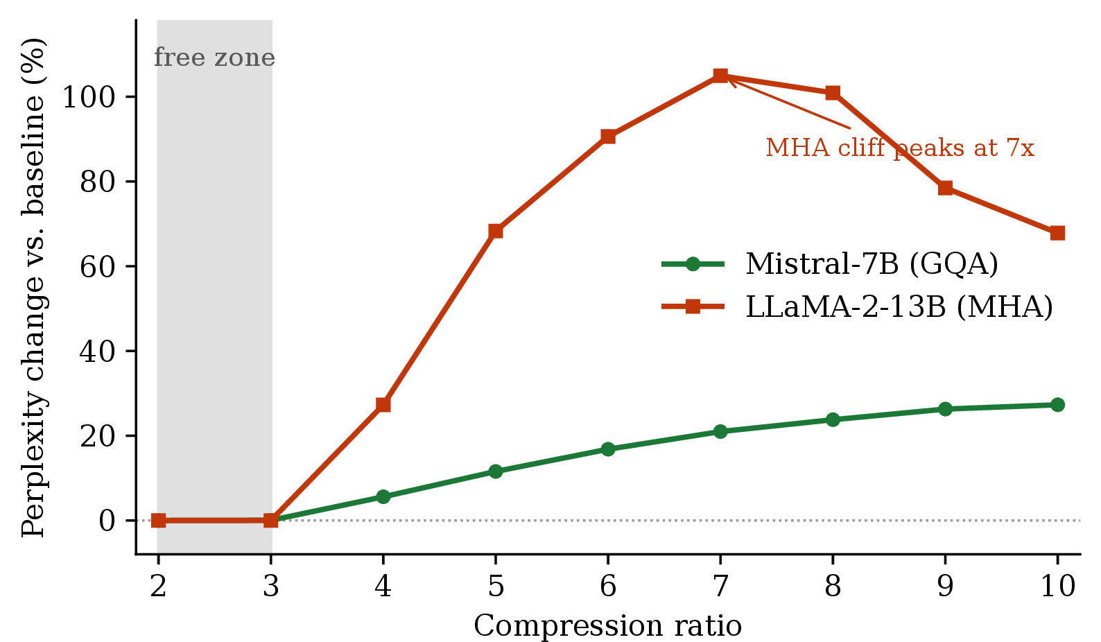
Our central claim is that a \(2\)–\(3\times\) cache is essentially free, and Figure 1 together with Table 1 shows it for perplexity. At \(2\)–\(3\times\) the drift stays within noise on both architectures at context lengths 512 and 1024; the only exception is the MHA model at ctx-2048, where \(2\)–\(3\times\) sits about \(2.5\%\) above baseline (Appendix 14). Beyond the free zone the two architectures part ways. Mistral degrades gracefully, losing roughly \(4\%\) perplexity per integer ratio step from \(4\times\) on, whereas LLaMA degrades sharply between \(4\times\) and \(5\times\). We return to this split repeatedly, because it is the main caveat on an otherwise architecture-agnostic result.
| Model | baseline | \(2\times\) | \(3\times\) | \(4\times\) | \(5\times\) |
|---|---|---|---|---|---|
| Mistral-7B (GQA) | 6.28 | 6.28 (\(-0.02\%\)) | 6.29 (\(+0.04\%\)) | 6.64 (\(+5.58\%\)) | 7.01 (\(+11.56\%\)) |
| LLaMA-2-13B (MHA) | 5.39 | 5.39 (\(-0.01\%\)) | 5.39 (\(-0.01\%\)) | 6.86 (\(+27.28\%\)) | 9.07 (\(+68.30\%\)) |
6.0.0.3 Reconstruction fidelity.
The free zone is so flat because JoLT reconstructs the cache far more faithfully than the baselines at the same budget. Table 2 reports relative Frobenius error at \(2\times\), where JoLT reaches \(0.009\) on keys and \(0.006\) on values, identically on both architectures and roughly an order of magnitude below both 4-bit quantization and cross-layer SVD. We stress that this error is small but nonzero everywhere, which is why we describe the regime as near-lossless rather than lossless.
| Mistral-7B (GQA) | LLaMA-2-13B (MHA) | |||
| Method | K | V | K | V |
| JoLT (ours) | 0.009 | 0.006 | 0.009 | 0.006 |
| int4 per-token | 0.080 | 0.131 | 0.077 | 0.123 |
| xKV (cross-layer SVD) | 0.077 | 0.237 | 0.087 | 0.224 |
6.0.0.4 Downstream tasks.
Low reconstruction error is only useful if it survives to task accuracy, so we evaluate the free zone end to end with the production fast method. On GSM8K [20], [21], scored with 8-shot chain-of-thought and exact match, every compressed cell at \(2\)–\(3\times\) lands within the Wilson \(95\%\) confidence interval of its baseline on both models: Mistral moves from \(40.56\%\) to \(39.04\%\) at \(2\times\) and \(38.44\%\) at \(3\times\) (full test set, \(n{=}1319\)), and LLaMA from \(28.13\%\) to \(29.04\%\) at \(2\times\) (\(n{=}1319\)). On RULER [22] single-needle retrieval (250 tasks per cell), Mistral holds exactly \(100\%\) at \(2\times\) and \(3\times\), and LLaMA matches its own ctx-4096 ceiling of \(84.8\%\) at \(2\times\) and \(83.6\%\) at \(3\times\). The architecture split reappears above the free zone, and it is starker for reasoning than for retrieval: LLaMA GSM8K falls to \(18.5\%\), \(6.0\%\), and \(1.5\%\) at \(4\times\), \(6\times\), and \(8\times\) (Appendix 15), the downstream face of its perplexity degradation, whereas Mistral RULER retrieval matches the full-KV baseline out to 16K context, at \(100\%\) at 8K and \(99.2\%\) at 16K.
7 Ablations↩︎
We now isolate the design choices behind the free zone. All ablations are on Mistral, with perplexity averaged over seeds \(\{0,1,2\}\) at \(T{=}1024\); the full grids over context lengths \(\{512, 1024, 2048\}\) are in Appendix 16, and the headline cells appear in Table 3.
The first question is whether the residual and the joint allocation matter, or whether a simpler scheme would do. They do matter. Removing the residual entirely, so that only Tucker ranks are allocated, costs about \(0.4\)–\(1.0\) PPL across the grid (for example \(7.27\) against \(6.54\) at \(2\times\)), which confirms that the residual is what makes the backbone near-lossless. Replacing the joint dual with a greedy allocator, which spends each marginal byte on whichever group offers the largest error reduction per byte but has no global multiplier to rebalance across keys and values, is more competitive at low ratio, where the two are within noise, but the joint solve pulls clearly ahead in the high-compression regime, for example \(7.92\) against \(8.36\) at \(8\times\) and \(T{=}512\), precisely where the freedom to move budget between keys and values is most valuable.
The second question is whether ranks should vary per group or be shared. Per-group allocation wins at every cell, by as much as \(0.97\) PPL at \(R{=}4\) and \(T{=}512\); the advantage shrinks at long context but never reverses, which tells us that different layer groups genuinely want different ranks.
The third question is how many residual bits are needed. Quality saturates at four bits: moving from \(0\) to \(2\) to \(4\) bits closes nearly all of the gap to near-lossless, while moving from \(4\) to \(8\) buys nothing measurable (\(6.537\) against \(6.536\) PPL at \(2\times\)). Since an 8-bit residual also cannot fit the byte budget above \(2\times\), four bits is both the quality knee and the only feasible default, which is why JoLT fixes the residual at four bits and lets the allocator decide only whether to spend them.
| \(2\times\) | \(4\times\) | \(8\times\) | |
|---|---|---|---|
| A1: allocation strategy | |||
| Joint (ours) | 6.54 | 6.93 | 8.14 |
| Greedy | 6.54 | 6.72 | 8.42 |
| Rank-only (no residual) | 7.27 | 7.95 | 8.65 |
| A5: rank allocation | |||
| Joint (per-group) | 6.54 | 6.93 | 8.14 |
| Uniform rank | 6.70 | 7.47 | 8.68 |
| Bit-grid: residual bits at \(2\times\) (0 / 2 / 4 / 8 bit) | |||
| PPL | \(7.27 \;/\; 6.63 \;/\; 6.537 \;/\; 6.536\) | ||
Two further ablations sit in the appendix because they confirm rather than establish design choices: the parity between the fast and exact backbones (Appendix 13), and the pre- versus post-RoPE capture point for keys (Appendix 12).
8 Memory Efficiency↩︎
The memory win is the persistent KV footprint, which shrinks to exactly the target ratio: on Mistral at ctx-2048 the cache drops from \(268.4\) MB to \(134.6\), \(89.6\), \(67.1\), and \(33.7\) MB at \(2\times\), \(3\times\), \(4\times\), and \(8\times\). Peak process memory, by contrast, is bounded by the model weights and activations and barely moves with the ratio, holding around \(16.5\) GB at ctx-2048. The footprint that shrinks is therefore the persistent state, which is exactly what matters for prompt-caching deployments that keep many cached prefixes resident at once. Decode reconstructs the compressed cache from its Tucker factors at each step, an arithmetic cost that today’s attention kernels are not built to absorb; a fused kernel that runs attention directly on the factors, without materializing the cache, is the natural route to decode parity and the main systems direction we leave open.
9 Conclusion↩︎
We presented JoLT and FlashJoLT, a KV-cache compressor that treats the cache at a layer as a third-order tensor, compresses only the token and feature axes that carry redundancy, and restores the rest with a JL-rotated low-bit residual, allocating ranks and residual bits jointly per layer group and per key/value through one Lagrangian dual. The central empirical result is a near-lossless \(2\)–\(3\times\) free zone that holds across perplexity, GSM8K, and RULER on both a GQA and an MHA model, supported at the representation level by an order-of-magnitude reduction in reconstruction error over strong baselines, and the fast variant FlashJoLT makes the method practical by cutting compression time \(5\)–\(13\times\) at matched quality.
Two boundaries scope these results and point to the next steps. First, the method is bounded by architecture at high ratio: grouped-query attention degrades gracefully past the free zone, but multi-head attention degrades sharply above \(4\times\) in both reconstruction and reasoning, so the safe, model-agnostic recommendation is the \(2\)–\(3\times\) band, and pushing MHA further will require an architecture-aware backbone. Second, the method is bounded by deployment cost: decode reconstructs the cache from its factors at each step, so a fused reconstruction-and-attention kernel that avoids materialization is the gap between a storage win and a deployable inference path, and the most important direction for future work. Two further caveats are worth stating directly. The compressed LLaMA RULER setting does not fit in 40GB because of the transient reconstruction copy and was run on larger hardware, a cost the same fused kernel would remove; and our byte accounting uses an fp16 serialization convention for the low-rank factors and idealized bit-packed bytes for the quantization baselines, so rankings within a class are exact while cross-class achieved ratios are convention-based. Validating calibration robustness across text domains is in progress, and the long-context cap policy is currently validated to 8192 tokens. Finally, this study was conducted under a single-GPU (A100-40GB) compute budget; broader sweeps, larger models, and the harder multi-needle long-context regime are left to future work with more compute.
10 Spectral structure (full)↩︎
Mistral-7B layer 15, \(T{=}1024\), mode-\(k\) SVD of each unfolding.
| Tensor | Mode | \(\sigma_1/\sigma_{\min}\) | \(r\) for \(\le 10\%\) | \(r\) for \(\le 20\%\) |
|---|---|---|---|---|
| K | heads (8) | 1.5 | 8/8 | 8/8 |
| K | tokens (1024) | 412 K | 228/1024 | 92/1024 |
| K | features (128) | 27.4 | 101/128 | 70/128 |
| V | heads (8) | 1.4 | 8/8 | 8/8 |
| V | tokens (1024) | 957 K | 563/1024 | 368/1024 |
| V | features (128) | 2.7 | 126/128 | 117/128 |
11 Mode pinning: per-head SVD and format comparison↩︎
11.1 Tucker vs.per-head SVD↩︎
On Mistral, over all layers at \(T{=}1024\) and matched storage, Tucker beats per-head SVD only when the head mode is left untruncated (\(r_1{=}n_{kv}\)).
| Ratio | K Tucker | K SVD | V Tucker | V SVD |
|---|---|---|---|---|
| 1.9\(\times\) | 0.081 | 0.130 | 0.260 | 0.400 |
| 3.8\(\times\) | 0.143 | 0.225 | 0.424 | 0.574 |
| 5.1\(\times\) | 0.241 | 0.267 | 0.606 | 0.638 |
| 9.8\(\times\) | 0.269 | 0.349 | 0.667 | 0.750 |
On LLaMA, configurations that compress the head mode (\(r_1 < n_{kv}\)) lose to per-head SVD, which confirms that the 3D advantage comes from sharing bases across heads rather than from reducing head-mode dimensionality. The layer mode behaves the same way: ablating the cross-layer rank to \(r_L \in \{2, 3\}\) below the layer count is catastrophic, raising key error \(2.5\)–\(11\times\), which is why the method pins both modes.
11.2 Multilinear format comparison↩︎
The mean relative Frobenius error over all layers and three seeds shows Tucker is the best multilinear format at every ratio on both architectures.
| Tucker | CP | t-SVD | TT | |||||
| Ratio (Mistral) | K | V | K | V | K | V | K | V |
| 2\(\times\) | 0.087 | 0.279 | 0.098 | 0.301 | 0.147 | 0.427 | 0.224 | 0.552 |
| 3\(\times\) | 0.125 | 0.381 | 0.155 | 0.436 | 0.204 | 0.543 | 0.303 | 0.674 |
| 5\(\times\) | 0.176 | 0.503 | 0.224 | 0.574 | 0.268 | 0.655 | 0.387 | 0.779 |
The ordering is Tucker \(<\) CP \(<\) t-SVD \(<\) TT on Mistral, and Tucker \(<\) t-SVD \(<\) TT on LLaMA, where CP is computationally intractable on the larger MHA tensor. Even the best multilinear format reaches value error around \(0.28\) at \(2\times\), far above JoLT’s \(0.006\), which is direct evidence that decomposing the small index-like modes is intrinsically lossy and that the win comes from the partial decomposition plus residual. Consistently, the full four-mode allocator, given complete freedom, reproduces the partial method byte for byte by driving the head and layer ranks to full size, which confirms the mode-pinning design.
12 RoPE pre vs.post on K↩︎
With the same groups and two compression passes (Mistral, \(T{=}1024\)), post-RoPE keys are uniformly harder to compress.
| Ratio | pre err\(_K\) | post err\(_K\) | gap % |
|---|---|---|---|
| 2\(\times\) | 0.0095 | 0.0162 | \(+70\%\) |
| 3\(\times\) | 0.0379 | 0.0489 | \(+29\%\) |
| 4\(\times\) | 0.1413 | 0.1861 | \(+32\%\) |
| 6\(\times\) | 0.2452 | 0.3140 | \(+28\%\) |
| 8\(\times\) | 0.2725 | 0.3543 | \(+30\%\) |
RoPE smears key energy off the top components in both the token and feature modes, dropping the group-0 top-8 feature-mode energy share from \(73.4\%\) to \(48.4\%\). The penalty replicates on LLaMA at \(+22\)–\(44\%\), which is why JoLT decomposes keys before RoPE and re-applies the rotation at decode time.
13 Fast variant: speedup and cap calibration↩︎
13.0.0.1 Compression-time speedup (Mistral, \(T{=}1024\), \(q_{\mathrm{cap}}{=}32\)).
| Target \(R\) | 2 | 3 | 4 | 5 | 6 | 7 | 8 | 10 |
|---|---|---|---|---|---|---|---|---|
| speedup | 8.87\(\times\) | 9.30\(\times\) | 5.25\(\times\) | 7.76\(\times\) | 6.87\(\times\) | 13.57\(\times\) | 7.57\(\times\) | 12.86\(\times\) |
LLaMA gives \(5.24\)–\(9.97\times\) at \(T{=}1024\), and the fast-versus-exact reconstruction parity in the free zone is \(|\Delta_K| \le 0.0093\) and \(|\Delta_V| \le 0.0011\) at \(2\)–\(3\times\).
13.0.0.2 Cap calibration gate (Mistral, real KV).
The policy passes the \(\Delta_K \le 0.025\), speedup \(\ge 3\times\) gate across the free zone (\(R \le 5\)) at every context from 512 to 8192. The token-mode effective rank grows sublinearly in \(T\), with the key rank-to-\(T\) fraction falling from \(0.355\) at \(T{=}512\) to \(0.066\) at \(T{=}8192\) and the value fraction from \(0.722\) to \(0.219\), so the feared eff-rank-proportional-to-\(T\) regime does not hold for real KV and the linear cap is a safe over-provision. The remaining failures are confined to small \(T\) at high ratio (\(R \ge 6\)), outside the free zone, where no reachable cap helps because the limit is high-ratio residual lossiness rather than cap size.
14 Full perplexity grids↩︎
Production fast method, multi-seed; \(\Delta\%\) is relative to the uncompressed baseline.
| Ratio | ctx=512 | ctx=1024 | ctx=2048 |
|---|---|---|---|
| baseline | 6.96 | 6.28 | 6.01 |
| 2\(\times\) | 6.96 (\(+0.07\%\)) | 6.28 (\(-0.02\%\)) | 5.98 (\(-0.42\%\)) |
| 3\(\times\) | 6.97 (\(+0.11\%\)) | 6.29 (\(+0.04\%\)) | 5.99 (\(-0.34\%\)) |
| 4\(\times\) | 7.26 (\(+4.37\%\)) | 6.64 (\(+5.58\%\)) | 6.26 (\(+4.21\%\)) |
| 5\(\times\) | 7.78 (\(+11.80\%\)) | 7.01 (\(+11.56\%\)) | 6.50 (\(+8.27\%\)) |
| 8\(\times\) | 8.54 (\(+22.69\%\)) | 7.78 (\(+23.77\%\)) | 7.10 (\(+18.23\%\)) |
| 10\(\times\) | 8.93 (\(+28.36\%\)) | 8.00 (\(+27.29\%\)) | 7.41 (\(+23.38\%\)) |
| Ratio | ctx=512 | ctx=1024 | ctx=2048 |
|---|---|---|---|
| baseline | 5.95 | 5.39 | 5.19 |
| 2\(\times\) | 5.95 (\(+0.04\%\)) | 5.39 (\(-0.01\%\)) | 5.32 (\(+2.54\%\)) |
| 3\(\times\) | 5.96 (\(+0.08\%\)) | 5.39 (\(-0.01\%\)) | 5.32 (\(+2.58\%\)) |
| 4\(\times\) | 6.78 (\(+13.94\%\)) | 6.86 (\(+27.28\%\)) | 6.44 (\(+24.17\%\)) |
| 5\(\times\) | 10.76 (\(+80.70\%\)) | 9.07 (\(+68.30\%\)) | 7.82 (\(+50.84\%\)) |
| 7\(\times\) | 13.28 (\(+123.10\%\)) | 11.04 (\(+104.94\%\)) | 8.53 (\(+64.41\%\)) |
| 10\(\times\) | 11.34 (\(+90.47\%\)) | 9.04 (\(+67.82\%\)) | 7.17 (\(+38.32\%\)) |
15 Downstream details↩︎
15.0.0.1 GSM8K degradation past the free zone (LLaMA-2-13B, fast method).
The baseline is \(28.13\%\) (\(n{=}1319\)) and \(2\times\) holds at \(29.04\%\) (\(n{=}1319\)), while \(4\times\), \(6\times\), and \(8\times\) fall to \(18.50\%\), \(6.00\%\), and \(1.50\%\) (\(n{=}200\) each). At \(2\times\) accuracy matches the baseline within noise; above the free zone it collapses, which is the downstream face of the MHA perplexity degradation.
15.0.0.2 Long-context RULER (Mistral, fast method).
Single-needle retrieval stays at \(100\%\) at \(2\times\) and \(3\times\) for ctx-8192 and at \(99.20\%\) for ctx-16384, matching the full-KV baseline at each context, where the \(0.8\)pp dip at 16K is present in the baseline as well. Achieved ratios land exactly on target.
16 Full ablation grids↩︎
A1 (joint / greedy / rank-only) and A5 (joint / uniform) report mean PPL over 3 seeds across all contexts; the joint, greedy, rank-only, and uniform allocators are defined in Section 7.
| ctx, ratio | joint | greedy | rank-only |
|---|---|---|---|
| 512, 2\(\times\) | 6.532 | 6.534 | 7.412 |
| 512, 8\(\times\) | 7.917 | 8.362 | 8.463 |
| 1024, 2\(\times\) | 6.536 | 6.535 | 7.269 |
| 1024, 4\(\times\) | 6.928 | 6.717 | 7.946 |
| 1024, 8\(\times\) | 8.145 | 8.418 | 8.649 |
| 2048, 2\(\times\) | 5.981 | 5.981 | 6.394 |
| 2048, 8\(\times\) | 7.102 | 7.057 | 7.388 |
| ctx, ratio | joint | uniform |
|---|---|---|
| 512, 2\(\times\) | 6.532 | 6.843 |
| 512, 4\(\times\) | 6.777 | 7.749 |
| 1024, 2\(\times\) | 6.536 | 6.702 |
| 1024, 8\(\times\) | 8.144 | 8.680 |
| 2048, 2\(\times\) | 5.981 | 6.059 |
| 2048, 8\(\times\) | 7.102 | 7.185 |