Symbolic Weak-form Recovery of 2-D Stochastic Generators
July 14, 2026
Abstract
Recovering two-dimensional Itô generators from trajectory data is difficult because drift increments have low signal-to-noise, bivariate weak designs can be ill-conditioned, and unconstrained tensor estimates need not be positive semidefinite. We study WG-SINDy estimator combining covariance-shaped spatial kernels, a ridge-stabilized local-polynomial projection, adaptive-LASSO/STLSQ selection, one in-sample per-component feasible diagonal GLS pass, and a PSD projection–Cholesky read-out with mild isotropic shrinkage. The released estimator uses a data-dependent full-cloud smoother and one in-sample per-component feasible diagonal GLS pass; accordingly, we do not claim exact finite-sample martingale cancellation or a feasible-GLS efficiency theorem for the reported implementation. We evaluate the estimator on 29 synthetic two-dimensional systems: 19 meet their declared per-system recovery contracts, eight are retained as named limits, and two remain scoped reviews. Across the 19 PASS rows, the median central-grid drift metric is 0.204 and the median tensor error is 0.0397. Among the six systems with a finite, non-degenerate off-diagonal target, the median \(a_{12}\) cosine is 0.997. Positive-semidefinite validity is imposed by construction. These results are synthetic, in-sample sampled-region diagnostics and do not establish universal or real-data recovery.
1 Introduction↩︎
A central problem across quantitative finance, molecular dynamics, neuroscience, and climate modelling is the inverse problem for stochastic dynamics: given a discretely sampled trajectory of a system, reconstruct the stochastic differential equation that generated it. The object that fully characterises a diffusion’s local dynamics is its infinitesimal generator \(\mathcal{L}f = b\!\cdot\!\nabla f + \tfrac{1}{2}\,a\!:\!\nabla^2 f\), encoding drift \(b\) and diffusion tensor \(a= \sigma\sigma^\top\). Recovering \(\mathcal{L}\) symbolically (rather than as a black-box surrogate) exposes spectral gaps, escape rates, leverage correlations, and drift-curl diagnostics directly.
The weak-form spatial-kernel estimator of Eshwar and Honnavar [1] addresses this problem in one dimension. For fixed or independently constructed spatial weight functions, projecting increments onto functions of the current state preserves the usual martingale cancellation: the weight evaluated at \(X_{t_n}\) is \(\mathcal{F}_{t_n}\)-measurable, so its product with the next Brownian increment has mean zero. The released estimator additionally learns its normalization, centres, bandwidths, and local-polynomial projection from the sampled state cloud; exact finite-sample cancellation is therefore not asserted for that data-dependent smoother.
Extending this to genuinely two-dimensional, coupled, non-diagonal diffusions is harder than it looks. A component-wise port of the 1D estimator to 2D (the “naive port” any reader would try first) fails on three fronts: the design matrix built from raw bivariate monomials over a scale-disparate, localised state cloud is severely ill-conditioned; the unweighted normal equations are statistically inefficient at low drift signal-to-noise; and the recovered diffusion tensor need not be positive semidefinite. We show these failures explicitly (4.2) and address them with targeted modifications.
1.0.0.1 Contributions
(i) Our algorithm is a weak-form 2D generator estimator that recovers both drift components and all three independent entries of the diffusion tensor symbolically inside the declared scope (3). (ii) We separate the fixed-weight spatial martingale identity from the released estimator, whose standardization, kernel geometry, local-polynomial projection, and feasible diagonal GLS weights are learned from the sampled state cloud. An independently constructed smoother-and-weight variant would recover exact cancellation, but that variant is not used in the reported experiments. (iii) The ablation identifies strong in-scope contributions from pooling, feasible GLS, and local-polynomial smoothing; the remaining components provide structural guarantees or protection in stress regimes (4.3). (iv) We evaluate the frozen estimator on 29 2D systems with per-system datasheets (¿sec:app:datasheets?) and an explicit falsification boundary.
1.1 Scope of claims↩︎
We claim recovery over a broad class of identifiable 2D Itô diffusions: those whose drift and diffusion lie in the chosen feature library, whose trajectories cover the state space, and whose design matrix has full column rank. We do not claim universal 2D recovery. We name, and do not paper over, the limits where recovery fails: the risk-neutral log-price drift \(\mu-\tfrac12 v\) of stochastic-volatility models (a low per-step signal whose squared signal-to-noise can be near \(10^{-4}\) in the simulated regime), near-singular and rank-deficient diffusion tensors, Feller-violating boundaries, non-spanning libraries, and under-covered state spaces. The diffusion tensor (not \(\sigma\) itself) is the identifiable object, since \(\sigma\) and \(\sigma O\) for any orthogonal \(O\) produce the same \(a=\sigma\sigma^\top\).
1.2 Code and data availability↩︎
The repository contains the estimator, experiment code, checked-in aggregate CSVs, and manuscript assets. Full raw campaign outputs and the external baseline snapshot are not included in this release; consequently, the current package supports audit of the checked-in aggregates but not bit-for-bit regeneration of every historical result. The repository is available at:
https://github.com/Sathvik-Gullipalli/Symbolic-Weak-form-Recovery-of-2-D-Stochastic-Generators.
2 Background↩︎
2.1 Itô stochastic differential equations↩︎
We consider a two-dimensional state \(X_t = (X_t^{(1)}, X_t^{(2)})^\top \in \mathbb{R}^2\) evolving as an Itô diffusion, \[\mathrm{d}X_t = b(X_t)\,\mathrm{d}t + \sigma(X_t)\,\mathrm{d}W_t, \label{eq:ito95sde}\tag{1}\] where \(b:\mathbb{R}^2\to\mathbb{R}^2\) is the drift vector, \(\sigma:\mathbb{R}^2\to\mathbb{R}^{2\times m}\) is the noise-loading matrix, and \(W_t\) is an \(m\)-dimensional Brownian motion. The drift governs the average direction of motion; the diffusion part controls the random fluctuations around it.
The local noise covariance is the diffusion tensor \(a(x) = \sigma(x)\sigma(x)^\top\), which in two dimensions is the symmetric matrix \[a(x) = \begin{pmatrix} a_{11}(x) & a_{12}(x) \\ a_{12}(x) & a_{22}(x) \end{pmatrix}.\] The diagonal entries \(a_{11}\), \(a_{22}\) are the local variances of the two coordinates. The off-diagonal entry \(a_{12}\) measures instantaneous coupling between the two noise shocks; in a stochastic volatility model it carries the leverage dependence between return and variance shocks.
Recovering the system from trajectory data means identifying five scalar functions: \(b_1\), \(b_2\), \(a_{11}\), \(a_{12}\), and \(a_{22}\).
2.2 From one-dimensional to two-dimensional SDEs↩︎
In one dimension the recovery problem has only two unknowns: a scalar drift \(b(x)\) and a local variance \(a(x) = \sigma^2(x)\). The two-dimensional case is structurally different. The drift becomes a vector of two functions, each potentially depending on both state variables, so the motion of one coordinate can influence the other. The noise becomes a full \(2\times 2\) tensor rather than a scalar.
The off-diagonal entry \(a_{12}\) has no analogue in scalar SDEs and cannot be recovered from marginal variances alone. A method that works for a 1D SDE does not automatically handle the 2D problem: the estimator must recover multiple drift components, cross-variation terms, and a diffusion tensor that qualifies as a covariance object.
2.3 The infinitesimal generator↩︎
The infinitesimal generator of 1 acts on smooth test functions \(f:\mathbb{R}^2\to\mathbb{R}\) by \[\mathcal{L}f = b_1\partial_1 f + b_2\partial_2 f + \tfrac{1}{2} \bigl( a_{11}\partial_{11}f + 2a_{12}\partial_{12}f + a_{22}\partial_{22}f \bigr). \label{eq:generator}\tag{2}\] The first-order terms are controlled by the drift; the second-order terms by the diffusion tensor. Recovering \(\mathcal{L}\) symbolically means identifying which candidate library functions \(\{\theta_k\}\) appear in each coefficient, under a sparsity assumption on those coefficients.
2.4 Why direct increment regression is difficult↩︎
The natural approach is to regress increments \(\Delta X_n / \Delta t\) directly on library features. The problem is that the Brownian noise term scales as \(1/\sqrt{\Delta t}\), so a single increment is a very noisy observation of the drift, and the noise grows as the sampling interval shrinks. Products of increments, used for the diffusion tensor, carry similar bias from finite-step effects and observation noise.
Weak-form methods avoid this by averaging many increments against spatial test functions. A properly chosen spatial weight reduces the martingale noise while preserving the identity linking averaged increments to the drift and diffusion coefficients.
2.5 The 1D weak-form spatial-kernel estimator↩︎
The estimator of [1] places Gaussian kernels \(K_j\) over the observed state range. Each kernel acts as a soft local bin, weighting increments by proximity to its centre. Drift and diffusion coefficients are then recovered by solving a shared linear system built from these weighted sums.
The reason this works is adaptedness: \(K_j(X_{t_n})\) depends only on information up to time \(t_n\) and is \(\mathcal{F}_{t_n}\)-measurable. The future Brownian increment is independent of \(\mathcal{F}_{t_n}\), so \[\mathbb{E}\!\left[ K_j(X_{t_n})\sigma(X_{t_n})(W_{t_{n+1}}-W_{t_n}) \,\middle|\, \mathcal{F}_{t_n} \right] = 0. \label{eq:tower95property}\tag{3}\] This martingale cancellation removes the Brownian noise without the bias that arises when test functions depend on future path values. In practice, finite-step bias correction and lag-one observation-noise correction are also applied.
2.6 What changes in two dimensions↩︎
Extending to two dimensions is not simply running the same regression twice. The off-diagonal coefficient \(a_{12}\) controls instantaneous cross-noise coupling and is invisible to methods that estimate only marginal variances. A valid extension must preserve the martingale identity 3 , recover all five generator coefficient fields, and return a diffusion tensor that is positive semidefinite.
Our algorithm keeps the spatial weak-form identity and extends the regression target to the full two-dimensional tensor, remaining derivative-free, sparse, symbolic, and generator-based.
2.7 Related methods↩︎
Sparse equation discovery is closely associated with SINDy, which uses sparse regression over a candidate function library to identify parsimonious governing equations [2]. Our regression stage also uses sequential thresholding and adaptive \(\ell_1\) regularization; the latter follows the adaptive-LASSO principle of assigning coefficient-specific penalty weights from an initial estimate [3], [4]. The local-polynomial projection used to reduce boundary bias is related to classical local-polynomial regression and smoothing [5].
For stochastic systems, Kramers–Moyal and stochastic-SINDy estimators use conditional increment moments to estimate drift and diffusion [6]. These estimators provide natural local-moment baselines, although single-step drift targets remain noisy because the Brownian contribution dominates the \(O(\Delta t)\) drift signal at small sampling intervals. Weak SINDy reduces derivative sensitivity through weak formulations [7], but its standard formulation was developed for deterministic dynamics and does not directly impose the geometry of a full two-dimensional diffusion tensor.
Extended dynamic mode decomposition and generator-EDMD methods approximate Koopman or generator action on a chosen dictionary [8]. Their primary target is an operator representation rather than a jointly sparse symbolic drift vector and positive-semidefinite diffusion tensor. The present method instead targets the five generator coefficient fields while imposing a PSD tensor read-out.
The comparisons reported below use lightweight in-repository implementations of these methodological families. They are diagnostic baseline proxies, not reproductions certified by the original authors, and their trajectory budgets are not identical. Consequently, the comparisons indicate where the proposed estimator is competitive under the shipped configurations; they do not establish universal method-level superiority.
3 Methodology↩︎
We develop a weak-form estimator for two-dimensional Itô generators that extends the spatial-kernel construction of [1] from scalar diffusions to coupled, non-diagonal diffusion tensors. The method is motivated by the martingale identity obtained for fixed or independently constructed spatial weights. In the released implementation, however, the smoother is estimated from the full sampled state cloud, so exact finite-sample adaptedness and unbiasedness are not claimed. The principal two-dimensional challenge is the simultaneous recovery of five coefficient fields, \[b_1,\qquad b_2,\qquad a_{11},\qquad a_{12},\qquad a_{22},\] under scale disparity, heteroscedastic drift noise, finite-step bias, and the positive-semidefiniteness constraint on \(a=\sigma\sigma^\top\).
Throughout this section, we observe \(R\) independent trajectories \(\{X^{(r)}_{t_n}\}_{n=0}^{N}\) of the diffusion \[\mathrm{d}X_t = b(X_t)\,\mathrm{d}t + \sigma(X_t)\,\mathrm{d}W_t, \qquad X_t\in\mathbb{R}^2, \label{eq:method95sde}\tag{4}\] at uniform step size \(\Delta t\), where \[a(x)=\sigma(x)\sigma(x)^\top = \begin{pmatrix} a_{11}(x) & a_{12}(x)\\ a_{12}(x) & a_{22}(x) \end{pmatrix}.\] The infinitesimal generator is \[\mathcal{L}f(x) = b_1(x)\partial_1 f(x) + b_2(x)\partial_2 f(x) + \frac{1}{2} \left[ a_{11}(x)\partial_{11}f(x) + 2a_{12}(x)\partial_{12}f(x) + a_{22}(x)\partial_{22}f(x) \right]. \label{eq:method95generator}\tag{5}\] The target is not \(\sigma\) itself, which is identifiable only up to orthogonal rotation, but the tensor \(a=\sigma\sigma^\top\) and the drift vector \(b\).
We assume a sparse library representation. Let \[\Theta(x)= \bigl[\theta_1(x),\ldots,\theta_K(x)\bigr]\in\mathbb{R}^{1\times K}.\] For each drift component and tensor entry, \[b_i(x)=\Theta(x)c^{(i)},\qquad i\in\{1,2\}, \label{eq:drift95library}\tag{6}\] and \[a_{ij}(x)=\Theta(x)d^{(ij)},\qquad 1\leq i\leq j\leq2. \label{eq:tensor95library}\tag{7}\] The coefficient vectors are sparse. Recovery therefore reduces to estimating the five sparse coefficient vectors \[c^{(1)},\quad c^{(2)},\quad d^{(11)},\quad d^{(12)},\quad d^{(22)}.\]
3.1 Standing assumptions↩︎
The analysis is stated under the following conditions.
Assumption 1 (Identifiable two-dimensional diffusion).
**Ergodicity.* The diffusion 4 admits a unique stationary measure \(\mu\) and is ergodic with finite mixing time relative to the observation horizon \(N\Delta t\).*
**Regularity.* The drift \(b\) and noise loading \(\sigma\) are locally Lipschitz with at most linear growth. The library functions \(\theta_k\) and spatial kernels used below are bounded on the sampled region and sufficiently smooth for the Taylor expansions used in the local-polynomial projection.*
**Library realizability.* The true drift and diffusion tensor entries lie in the span of the chosen library as in 6 –7 . If this fails, the estimator returns the best weak-projection approximation in the chosen library, not the exact generator. The PSD Cholesky read-out in 3.7 additionally requires library-spanned Cholesky factor fields for exact symbolic read-out through that stage; otherwise the final tensor should be interpreted as a PSD approximation in the induced product library.*
**Coverage.* Each normalized smoother row receives non-vanishing effective horizon: \[T_{\mathrm{eff},j} = \frac{\Delta t}{\sum_{r,n}(\Pi_{j n}^{(r)})^2} \to\infty, \qquad \max_{r,n}|\Pi_{j n}^{(r)}|\to0 .\]*
**Full rank.* The population weak design matrix \[\bar A_{jk} = \int \pi_j(x)\theta_k(x)\,\mathrm{d}\mu(x)\] has full column rank on the active library support, where \(\pi_j\) denotes the population limit of the \(j\)th normalized local-polynomial intercept row.*
**Tensor consistency.* The first-pass tensor estimator satisfies \[\|\hat{a}-a\|_{\infty}=o_p(1).\]*
These assumptions define the population identifiability, coverage, and library envelope under which the weak system has a unique symbolic target. They do not, by themselves, establish exact finite-sample unbiasedness or consistency for the released data-dependent full-cloud smoother. The reported recovery evidence is therefore empirical and restricted to the declared sampled-region benchmark setting.
3.2 Why the naive 1D-to-2D port fails↩︎
The scalar estimator of [1] uses spatial Gaussian kernels to build a weak design matrix and then solves two sparse systems: one for the drift and one for the scalar diffusion. A direct 2D port would simply solve five independent systems over a bivariate library: \[b_1,\;b_2,\;a_{11},\;a_{12},\;a_{22}.\] This direct port fails for three structural reasons.
First, the raw bivariate design is ill-conditioned. If the two coordinates have aspect ratio \(\kappa\), then polynomial columns of degree \(d\) can differ in scale by \(O(\kappa^d)\). In stochastic-volatility data, for example, the log-price coordinate may be \(O(1)\)–\(O(10)\) while the variance coordinate may be \(O(10^{-2})\)–\(O(10^{-1})\). The resulting normal equations are unstable.
Second, the drift target is heteroscedastic across kernels. For Euler-generated benchmarks the sampled increment is \[\Delta X_n = b(X_{t_n})\Delta t + \sigma(X_{t_n})\Delta W_n, \label{eq:euler95increment}\tag{8}\] the drift signal scales as \(\Delta t\) while the Brownian noise scales as \(\sqrt{\Delta t}\). Kernels located in high-diffusion regions therefore carry much larger noise variance than kernels in low-diffusion regions. Ordinary least squares treats these rows as equally reliable.
Third, an unconstrained regression for \(a_{11},a_{12},a_{22}\) does not guarantee \[\hat{a}(x)\succeq0.\] A fitted tensor with negative eigenvalues cannot be interpreted as a local covariance. This is not cosmetic: it breaks the leverage read-out \(a_{12}/\sqrt{a_{11}a_{22}}\) and invalidates the generator as a diffusion generator.
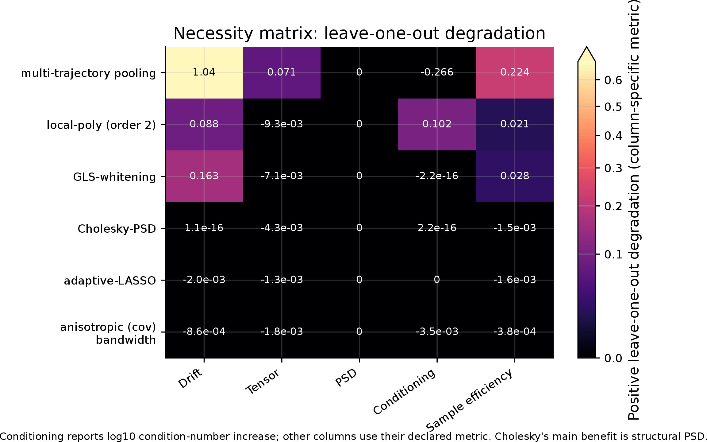
On top of the base weak-form construction (coordinate standardization, spatial Gaussian kernels, and the finite-step drift-square correction), the estimator adds six mechanisms, each targeting one of the failure modes above: (i) anisotropic covariance-shaped kernels, (ii) an order-2 local-polynomial weak projection, (iii) adaptive-LASSO sparsification, (iv) feasible generalized-least-squares drift reweighting, (v) a PSD Cholesky diffusion read-out, and (vi) multi-trajectory pooling. These six ingredients are examined through the cumulative-graft and leave-one-out analyses of 4.3. Pooling, feasible diagonal GLS, and local-polynomial smoothing show clear degradation when removed on the reported in-scope summary. The PSD Cholesky read-out, adaptive sparsification, and anisotropic bandwidths primarily provide structural validity or protection in stress regimes; the leave-one-out matrix does not establish that each is individually necessary for the in-scope median score.
3.3 Weak-form moment equations↩︎
For a smooth observable \(\phi\), Dynkin’s formula gives \[\mathbb{E}\!\left[ \phi(X_{t_{n+1}})-\phi(X_{t_n}) \,\middle|\, \mathcal{F}_{t_n} \right] = (\mathcal{L}\phi)(X_{t_n})\Delta t + O(\Delta t^2). \label{eq:dynkin95method}\tag{9}\] For Euler–Maruyama trajectories the sampled increment is exactly \[\Delta X_n = b(X_{t_n})\,\Delta t + \sigma(X_{t_n})\,\Delta W_n, \qquad \Delta W_n\sim\mathcal{N}(0,\Delta t\,I_m)\perp\mathcal{F}_{t_n}. \label{eq:euler95exact95method}\tag{10}\] Because the drift and noise loading are frozen at \(X_{t_n}\) over the step, the first two conditional moments are then exact. Taking \(\phi(x)=x^{(p)}\), \[\mathbb{E}\!\left[ \Delta X_n^{(p)} \,\middle|\, \mathcal{F}_{t_n} \right] = b_p(X_{t_n})\,\Delta t, \qquad p=1,2, \label{eq:drift95moment95method}\tag{11}\] and taking \(\phi(x)=x^{(p)}x^{(q)}\), using \(\mathbb{E}[\Delta W_n^{(k)}\Delta W_n^{(\ell)}\mid\mathcal{F}_{t_n}]=\delta_{k\ell}\Delta t\) and the mean-zero cross term, \[\mathbb{E}\!\left[ \Delta X_n^{(p)}\Delta X_n^{(q)} \,\middle|\, \mathcal{F}_{t_n} \right] = a_{pq}(X_{t_n})\,\Delta t + b_p(X_{t_n})b_q(X_{t_n})\,\Delta t^2 . \label{eq:diffusion95moment95method}\tag{12}\] Both identities are exact for Euler–Maruyama data. For a general continuous Itô diffusion sampled at spacing \(\Delta t\), or for exact-transition simulators such as the OU and GBM families used in the benchmark, they hold up to the corresponding finite-step conditional-moment remainder; for clipped or projected stress systems they describe the declared sampled process only on the retained sampled region. The estimator treats the Euler increment as the working model. The drift is therefore read from first increments, and the tensor from quadratic increments once the drift-square term \(b_pb_q\Delta t^2\) is removed (3.6).
Let \(\Pi\in\mathbb{R}^{J\times RN}\) denote the normalized spatial smoother matrix whose \(j\)th row locally averages quantities around centre \(c_j\). Let \(\Theta\in\mathbb{R}^{RN\times K}\) be the library matrix evaluated at all sampled states. The shared weak design matrix is For drift component \(p\), define \[B^{(p)} = \Pi\!\left(\frac{\Delta X^{(p)}}{\Delta t}\right). \label{eq:drift95target95method}\tag{14}\] For diffusion entry \((p,q)\), define the corrected pointwise target \[q_n^{(pq)} = \frac{1}{\Delta t} \left[ \Delta X_n^{(p)}\Delta X_n^{(q)} - \hat{b}_p(X_{t_n})\hat{b}_q(X_{t_n})\Delta t^2 \right], \label{eq:q95target95method}\tag{15}\] and smooth it: \[Q^{(pq)}=\Pi q^{(pq)}. \label{eq:tensor95target95method}\tag{16}\] The weak systems are then \[B^{(p)}\approx A c^{(p)}, \qquad Q^{(pq)}\approx A d^{(pq)}. \label{eq:weak95systems95method}\tag{17}\] Both drift and diffusion use the same \(A\). This is important: the method learns a single symbolic generator, not separate unrelated regressions.
3.4 Spatial weak rows and the dependence caveat↩︎
The spatial weak construction is motivated by a standard martingale identity. For one Euler-generated trajectory and one component, \[\Delta X_n^{(p)} = b_p(X_{t_n})\Delta t + \sum_{\ell}\sigma_{p\ell}(X_{t_n})\Delta W_n^{(\ell)}.\] Let \(\pi_j\) be a fixed deterministic spatial weight function. The corresponding martingale contribution is \[M_j^{(p)} = \sum_n \pi_j(X_{t_n}) \sum_{\ell} \sigma_{p\ell}(X_{t_n})\Delta W_n^{(\ell)}.\] Because \(\pi_j(X_{t_n})\sigma_{p\ell}(X_{t_n})\) is \(\mathcal{F}_{t_n}\)-measurable, \[\mathbb{E}\!\left[ \pi_j(X_{t_n}) \sigma_{p\ell}(X_{t_n}) \Delta W_n^{(\ell)} \,\middle|\, \mathcal{F}_{t_n} \right] = 0.\] Thus a fixed or independently constructed spatial weight preserves the usual martingale cancellation.
The released smoother is more data-dependent than this idealized calculation. Coordinate standardization, \(k\)-means centres, covariance-shaped bandwidths, and the local-polynomial Gram matrices are estimated from the full sampled state cloud. Consequently, a finite-sample entry \(\Pi_{jn}\) need not be \(\mathcal{F}_{t_n}\)-measurable, because it can depend on states observed after \(t_n\). The preceding tower-property calculation therefore motivates the population weak identity but does not establish exact finite-sample cancellation for the released full-cloud smoother.
An exactly cross-fitted construction would estimate all nuisance objects—standardization, centres, bandwidths, local-polynomial Gram matrices, the resulting spatial weight functions, and the first-pass diffusion field—using trajectories other than the trajectory on which the weak row is evaluated. The resulting weight function would then be fixed relative to the evaluated trajectory. This fully cross-fitted construction is not used in the reported experiments, so no numerical result in this paper is presented as evidence for such a theorem.
3.5 Standardization, anisotropic kernels, and local-polynomial projection↩︎
3.5.0.1 Standardization.
The states are standardized coordinate-wise before constructing kernels or libraries: \[z_n = S_{\mathrm{std}}^{-1}(X_{t_n}-\bar X), \qquad S_{\mathrm{std}}=\operatorname{diag}(s_1,s_2), \label{eq:standardization95method}\tag{18}\] where \(\bar X\) is the empirical mean and \(s_1,s_2\) are empirical marginal standard deviations. The library is evaluated in \(z\)-coordinates. After recovery, coefficients may be mapped back to physical coordinates by the exact polynomial change of variables induced by \[z=S_{\mathrm{std}}^{-1}(x-\bar X).\] This removes the axis-scale disparity that causes the raw bivariate monomial design to become ill-conditioned.
3.5.0.2 Kernel centres and bandwidth.
Centres \(\{c_j\}_{j=1}^{J}\) are placed by \(k\)-means on the standardized cloud \(\{z_n\}\). In the frozen implementation, \(J=64\). The covariance-shaped bandwidth is \[\Sigma_{\mathrm{bw}} = h_0^2 \frac{\widehat{\operatorname{Cov}}(z)}{\operatorname{tr}\widehat{\operatorname{Cov}}(z)/2} + 10^{-8}I, \qquad h_0 = 1.5\, \operatorname{median}_j \min_{j'\neq j}\|c_j-c_{j'}\|. \label{eq:bw95method}\tag{19}\] The unnormalized spatial kernel is \[w_{jn} = \exp\!\left[ -\frac{1}{2} (z_n-c_j)^\top \Sigma_{\mathrm{bw}}^{-1} (z_n-c_j) \right]. \label{eq:kernel95weight95method}\tag{20}\] Unlike an isotropic kernel, this kernel adapts to residual covariance structure in the standardized cloud.
3.5.0.3 Order-2 local-polynomial smoother.
A local-constant Nadaraya–Watson estimate at centre \(c_j\) is \[\hat{g}_{\mathrm{NW}}(c_j) = \frac{\sum_n w_{jn}g(z_n)}{\sum_n w_{jn}}. \label{eq:nw95method}\tag{21}\] Taylor expansion gives \[\mathbb{E}[\hat{g}_{\mathrm{NW}}(c_j)] = g(c_j) + \nabla g(c_j)^\top\nu_j + \frac{1}{2} \operatorname{tr} \left( \nabla^2 g(c_j)\Sigma_{\mathrm{bw}} \right) + O(h_0^4), \label{eq:nw95bias95method}\tag{22}\] where \[\nu_j=\mathbb{E}_{w_j}[z-c_j].\] In the interior \(\nu_j=0\), but near the boundary the kernel is truncated and \(\nu_j\neq0\), producing a first-order boundary bias.
To remove this leading bias, we use an order-2 local-polynomial projection. Let \[\delta_{jn}=z_n-c_j,\] and define the quadratic local basis \[r(\delta) = \begin{bmatrix} 1& \delta_1& \delta_2& \delta_1^2& \delta_1\delta_2& \delta_2^2 \end{bmatrix}^{\top}. \label{eq:local95poly95basis95method}\tag{23}\] For each centre \(c_j\), construct \[R_j = \begin{bmatrix} r(\delta_{j1})^\top\\ \vdots\\ r(\delta_{j,RN})^\top \end{bmatrix}, \qquad W_j=\operatorname{diag}(w_{j1},\ldots,w_{j,RN}).\] The local-polynomial fit for a target vector \(g\) solves \[\hat{\beta}_j(g) = \arg\min_{\beta} \sum_n w_{jn} \left[ g(z_n)-r(\delta_{jn})^\top\beta \right]^2 + \varepsilon_j\|\beta\|_2^2, \label{eq:local95poly95fit95method}\tag{24}\] where \(\varepsilon_j=10^{-8}\,\overline{\operatorname{diag}}(R_j^\top W_j R_j)\) is a small ridge scaled to the local Gram magnitude, present only for numerical stability. The estimate at the centre is the intercept: \[\hat{g}(c_j)=e_1^\top\hat{\beta}_j(g).\] Equivalently, the smoother row is \[\Pi_{j\cdot} = e_1^\top \left(R_j^\top W_j R_j+\varepsilon_j I\right)^{-1} R_j^\top W_j. \label{eq:smoother95row95method}\tag{25}\] Without the ridge term, the order-2 local-polynomial intercept reproduces all quadratic polynomials exactly and removes the first-moment and curvature terms in 22 . The stabilized implementation uses the nonzero ridge in 24 ; this adds a regularization bias controlled by \(\varepsilon_j\) that vanishes as the ridge scale tends to zero under stable local conditioning. Thus the projection bias is \(O(h_0^4)\) plus the ridge-induced term, not a pure \(O(h_0^4)\) bound at fixed ridge.
3.6 First-pass drift and finite-step tensor correction↩︎
The first-pass drift solves \[\hat{c}^{(p)}_{\mathrm{OLS}} = \arg\min_c \|B^{(p)}-Ac\|_2^2 + \lambda\|c\|_2^2, \qquad p=1,2, \label{eq:first95pass95drift95method}\tag{26}\] or the corresponding sparse version described in 3.9. This gives \[\hat{b}_p(x)=\Theta(x)\hat{c}^{(p)}.\]
The diffusion target must be corrected because quadratic increments contain a drift-squared finite-step contribution. For Euler-generated data, 12 gives the exact conditional identity \[\mathbb{E}\!\left[ \Delta X_n\Delta X_n^\top \,\middle|\, \mathcal{F}_{t_n} \right] = a(X_{t_n})\Delta t + b(X_{t_n})b(X_{t_n})^\top\Delta t^2. \label{eq:outer95expansion95method}\tag{27}\] For a continuously sampled Itô diffusion rather than an Euler benchmark, the same displayed expression carries the weak \(O(\Delta t^2)\) conditional-moment remainder from 9 . Therefore, for each tensor entry, \[q_n^{(pq)} = \frac{ \Delta X_n^{(p)}\Delta X_n^{(q)} - \hat{b}_p(X_{t_n})\hat{b}_q(X_{t_n})\Delta t^2 }{\Delta t}. \label{eq:finite95step95method}\tag{28}\] The smoothed tensor target is \[Q^{(pq)}=\Pi q^{(pq)}.\] Then \[\hat{d}^{(pq)} = \arg\min_d \|Q^{(pq)}-Ad\|_2^2 + \lambda\|d\|_2^2. \label{eq:tensor95ridge95method}\tag{29}\]
3.6.0.1 Optional observation-noise correction.
If observations are contaminated by additive noise, \[\widetilde{X}_n=X_n+\eta_n, \qquad \mathbb{E}[\eta_n]=0, \qquad \operatorname{Cov}(\eta_n)=\Sigma_{\eta},\] then lag-zero quadratic variation is inflated by \(2\Sigma_\eta\), while \[\mathbb{E}[ \Delta\widetilde{X}_n \Delta\widetilde{X}_{n+1}^{\top} ] = -\Sigma_\eta + o(1).\] Thus \(\Sigma_\eta\) can be estimated from the lag-one outer product and subtracted from the raw quadratic increment before division by \(\Delta t\): \[q_n = \frac{ \Delta\widetilde{X}_n\Delta\widetilde{X}_n^\top -2\hat{\Sigma}_\eta -\hat{b}(X_{t_n})\hat{b}(X_{t_n})^\top\Delta t^2 }{\Delta t}. \label{eq:obs95noise95corrected95target95method}\tag{30}\] In the reported clean synthetic benchmarks this correction is disabled to avoid adding unnecessary variance. For pooled trajectories, the lag-one estimator must be applied trajectory-aware so that artificial cross-trajectory pairs are not used.
3.7 PSD Cholesky diffusion read-out↩︎
A direct linear fit for \(a_{11},a_{12},a_{22}\) does not guarantee \(\hat{a}(x)\succeq0\). We therefore recover the tensor through a Cholesky read-out. The released implementation does not solve a nonlinear alternating least-squares problem directly in the Cholesky coefficients. Instead, it uses a three-stage procedure: first fit the unconstrained tensor entries, then project the pointwise tensor estimates to the PSD cone, and finally regress the corresponding Cholesky factor fields on the same library.
First, the unconstrained entrywise tensor estimate is evaluated at the data: \[\hat{a}_{\mathrm{lin}}(X_{t_n}) = \begin{pmatrix} \Theta(X_{t_n})\hat{d}^{(11)} & \Theta(X_{t_n})\hat{d}^{(12)} \\ \Theta(X_{t_n})\hat{d}^{(12)} & \Theta(X_{t_n})\hat{d}^{(22)} \end{pmatrix}.\] Each pointwise matrix is projected to the PSD cone by eigenvalue clipping: \[\hat{a}_{\mathrm{PSD}}(X_{t_n}) = \sum_{k=1}^{2} \max(\lambda_k,10^{-10})v_kv_k^\top, \label{eq:psd95projection95method}\tag{31}\] where \((\lambda_k,v_k)\) are the eigenpairs of \(\hat{a}_{\mathrm{lin}}(X_{t_n})\).
Next compute the pointwise Cholesky fields \[\begin{align} \ell_{11}(X_{t_n}) &= \sqrt{\hat{a}_{\mathrm{PSD},11}(X_{t_n})}, \tag{32}\\ \ell_{21}(X_{t_n}) &= \frac{ \hat{a}_{\mathrm{PSD},12}(X_{t_n}) }{ \ell_{11}(X_{t_n}) }, \tag{33}\\ \ell_{22}(X_{t_n}) &= \sqrt{ \hat{a}_{\mathrm{PSD},22}(X_{t_n}) - \ell_{21}(X_{t_n})^2 }, \tag{34} \end{align}\] with denominators and radicands floored at \(10^{-10}\).
Each Cholesky factor field is then weak-regressed against the same library: \[\ell_{ab}(x)=\Theta(x)\beta^{(ab)}, \qquad (a,b)\in\{(1,1),(2,1),(2,2)\}. \label{eq:chol95library95method}\tag{35}\] The coefficient vectors are obtained from \[\hat{\beta}^{(ab)} = \arg\min_{\beta} \|\Pi\ell_{ab}-A\beta\|_2^2 + \lambda\|\beta\|_2^2. \label{eq:chol95fit95method}\tag{36}\]
At read-out, define \[\hat{L}(x) = \begin{pmatrix} \hat{\ell}_{11}(x) & 0\\ \hat{\ell}_{21}(x) & \hat{\ell}_{22}(x) \end{pmatrix}.\] The recovered tensor is \[\hat{a}(x) = \hat{L}(x)\hat{L}(x)^\top, \label{eq:chol95tensor95method}\tag{37}\] or explicitly \[\begin{align} \hat{a}_{11}(x) &= \hat{\ell}_{11}(x)^2, \tag{38}\\ \hat{a}_{12}(x) &= \hat{\ell}_{11}(x)\hat{\ell}_{21}(x), \tag{39}\\ \hat{a}_{22}(x) &= \hat{\ell}_{21}(x)^2+\hat{\ell}_{22}(x)^2. \tag{40} \end{align}\] Thus \(\hat{a}(x)\succeq0\) for every \(x\) by construction. This stage is a PSD Cholesky read-out/approximation unless the Cholesky factor fields themselves are spanned by the chosen library. After expansion 38 –40 , the tensor entries belong to the induced product library, not necessarily to the original linear entrywise library.
Finally, the read-out tensor is mildly shrunk toward its isotropic part: \[\hat{a}(x) \leftarrow (1-\rho)\hat{a}(x) + \rho\, \frac{1}{2} \operatorname{tr}\bigl(\hat{a}(x)\bigr)I, \qquad \rho=0.05. \label{eq:isotropic95shrink95method}\tag{41}\] This stabilizes near-singular and low-coverage regimes while leaving well-identified tensor fields essentially unchanged.
3.8 Feasible generalized-least-squares drift reweighting↩︎
The first-pass drift weak system has the form \[B^{(p)}=Ac^{(p)}+M^{(p)}, \label{eq:drift95noise95model95method}\tag{42}\] where \(M^{(p)}\) is a martingale noise term. Although \(\mathbb{E}[M^{(p)}]=0\), its variance is not constant across kernel rows: rows centred in high-diffusion regions are noisier. The frozen estimator corrects this with a per-component diagonal feasible GLS pass, using the first-pass diffusion diagonal \(\hat{a}_{pp}\) to build the row weights. For row \(j\), the diagonal proxy for the drift-noise variance is \[V_j^{(p)} = \frac{1}{\Delta t} \sum_n \Pi_{jn}^2 \hat{a}_{pp}(X_{t_n}). \label{eq:noise95var95method}\tag{43}\] Rows in high-diffusion regions have larger \(V_j^{(p)}\) and should be down-weighted.
The feasible GLS row multiplier is \[s_j^{(p)} = \operatorname{clip}_{[0.05,\,20]} \left( \frac{(V_j^{(p)})^{-1/2}}{\operatorname{median}_{j'}(V_{j'}^{(p)})^{-1/2}} \right). \label{eq:gls95weight95method}\tag{44}\] Let \[W_p=\operatorname{diag}\left((s_1^{(p)})^2,\ldots,(s_J^{(p)})^2\right).\] The drift is re-estimated by \[\hat{c}^{(p)}_{\mathrm{GLS}} = (A^\top W_p A)^{-1}A^\top W_pB^{(p)}. \label{eq:gls95estimator95method}\tag{45}\] Equivalently, rows of \(A\) and \(B^{(p)}\) are scaled by \(s_j^{(p)}\) before solving. In the frozen configuration this reweighting is run for a single pass, and the clip in 44 caps the influence of extreme rows. The normal-equation weight is \(W_p\), so the row multiplier \(s_j^{(p)}\) corresponds to a squared weight in the GLS objective. The weights use only the diagonal \(\hat{a}_{pp}\), so they are diagonal GLS-style weights for the per-component heteroscedastic model rather than a full cross-component whitening; a full-tensor whitening variant, which also uses \(\hat{a}_{12}\), is available but is not part of the default stack.
3.8.0.1 Status of feasible diagonal GLS.
The released estimator performs one in-sample per-component feasible diagonal GLS pass. Its row weights are plug-in functions of the first-pass diffusion estimate and the data-dependent spatial projection. The pass is intended as a variance-stabilizing numerical reweighting and is evaluated through the ablation study. We do not claim exact finite-sample unbiasedness, asymptotic equivalence to oracle GLS, or attainment of oracle efficiency for this released implementation. Establishing those properties would require a fully independent or predictable construction of both the smoother and the GLS weights, together with additional rate and stochastic-equicontinuity conditions.
3.9 Adaptive LASSO, debiasing, and multi-trajectory pooling↩︎
Every weak system above is solved using the same sparse selection routine. First, the design columns are \(\ell_2\)-normalized. An initial ridge estimate \(\hat{c}^{\mathrm{init}}\) is computed, and adaptive penalty weights are set as \[\omega_k= \max\!\bigl(|\hat{c}_k^{\mathrm{init}}|,\,\epsilon_0\bigr)^{-\gamma}, \qquad \gamma=1, \qquad \epsilon_0=10^{-3}, \label{eq:adaptive95weights95method}\tag{46}\] where the floor \(\epsilon_0\) keeps the weight of a vanishing pilot coefficient finite. The penalty parameter \(\alpha\) is chosen by cross-validation. When trajectory identifiers are supplied, this cross-validation is grouped by trajectory; otherwise the implementation falls back to pseudo-block cross-validation over the projected weak rows. The adaptive-LASSO problem is \[\hat{c} = \arg\min_c \left\{ \frac{1}{2}\|y-Xc\|_2^2 + \alpha\sum_{k=1}^{K}\omega_k|c_k| \right\}. \label{eq:adaptive95lasso95method}\tag{47}\] Large pilot coefficients are penalized lightly; near-zero pilot coefficients are penalized heavily. This reduces the common failure mode of uniform LASSO: overshrinking true dominant terms while retaining small spurious terms.
After selection, the active support \[\hat{S}=\{k:\hat{c}_k\neq0\}\] is refit by ordinary least squares: \[\hat{c}_{\hat{S}}^{\mathrm{debias}} = \arg\min_u \|y-X_{\hat{S}}u\|_2^2, \qquad \hat{c}_{\hat{S}^c}^{\mathrm{debias}}=0. \label{eq:debias95method}\tag{48}\] A sequentially-thresholded least-squares pruning step then removes terms whose absolute coefficient is below a fixed relative threshold of the largest retained coefficient for that target, refitting after each pruning step. In the frozen estimator this internal threshold is \[\tau_{\mathrm{STLSQ}}=0.12.\] This \(12\%\) rule is the estimator’s actual sparsification threshold. It should be distinguished from the smaller \(10^{-3}\) threshold used later only for reporting whether a coefficient was nonzero in the coefficient-recovery table.
For multi-trajectory pooling, independent trajectories are pooled by stacking their weak rows. When trajectory identifiers are supplied to the estimator, each trajectory is smoothed separately, producing trajectory-specific rows \[A^{(r)},\quad B^{(r,p)},\quad Q^{(r,pq)}.\] The pooled systems are stacked: \[A_{\mathrm{pool}} = \begin{bmatrix} A^{(1)}\\ \vdots\\ A^{(R)} \end{bmatrix}, \qquad B_{\mathrm{pool}}^{(p)} = \begin{bmatrix} B^{(1,p)}\\ \vdots\\ B^{(R,p)} \end{bmatrix}. \label{eq:pooling95method}\tag{49}\] The same construction is used for \(Q^{(pq)}\). In this trajectory-aware mode, cross-validation is grouped by trajectory, so folds hold out whole trajectories rather than individual kernel rows.
The main coefficient-recovery rerun uses the same statistical idea of multi-trajectory pooling, but the released script stacks the \(R=32\) trajectories as a single pooled state-increment cloud before calling the estimator. Since that script does not pass trajectory identifiers, the sparse-selection routine uses its pseudo-block cross-validation fallback rather than one-fold-per-trajectory cross-validation. Thus the coefficient table should be read as evidence for the effect of pooled trajectory coverage and sample size, not as a trajectory-held-out CV experiment.
3.10 Symbolic generator read-out↩︎
The final recovered drift is \[\hat{b}(x) = \begin{pmatrix} \Theta(x)\hat{c}^{(1)}\\ \Theta(x)\hat{c}^{(2)} \end{pmatrix}.\] The final recovered diffusion tensor is the Cholesky read-out \[\hat{a}(x)=\hat{L}(x)\hat{L}(x)^\top.\] The symbolic generator is therefore \[\hat{\mathcal{L}}f(x) = \hat{b}_1(x)\partial_1 f(x) + \hat{b}_2(x)\partial_2 f(x) + \frac{1}{2} \left[ \hat{a}_{11}(x)\partial_{11}f(x) + 2\hat{a}_{12}(x)\partial_{12}f(x) + \hat{a}_{22}(x)\partial_{22}f(x) \right]. \label{eq:estimated95generator95method}\tag{50}\]
Three physically meaningful quantities are read directly from this generator: \[\begin{align} \text{leverage}(x) &= \frac{\hat{a}_{12}(x)}{\sqrt{\hat{a}_{11}(x)\hat{a}_{22}(x)}}, \tag{51}\\ \text{fluctuation fields}(x) &= \bigl(\hat{a}_{11}(x),\hat{a}_{22}(x)\bigr), \tag{52}\\ \text{drift curl}(x) &= \frac{1}{2} \left( \partial_1\hat{b}_2(x) - \partial_2\hat{b}_1(x) \right). \tag{53} \end{align}\] The implementation also reports the antisymmetric-drift field \(x\mapsto x\,\operatorname{anti}(\nabla\hat{b}(x))^\top\) as a directional diagnostic. In the isotropic rotational OU case this diagnostic is analytically aligned with the stationary current direction. For state-dependent diffusion or general nonlinear systems it is not the full stationary Fokker–Planck current \(J=b\pi-\tfrac12\nabla\cdot(a\pi)\), which would require density estimation and the diffusion-divergence term.
3.11 Metrics and support rule↩︎
All reported field errors are equal-weight relative \(L^2\) errors on a Cartesian grid \(\mathcal{G}\) spanning the coordinatewise 2nd–98th percentiles of the trajectories used for fitting. They are in-sample, sampled-region diagnostics rather than stationary-measure-weighted or held-out errors. For a scalar field \(g\), \[\operatorname{err}_{\mathcal{G}}(\hat{g},g) = \left[ \frac{\sum_{x\in\mathcal{G}}(\hat{g}(x)-g(x))^2}{\sum_{x\in\mathcal{G}}g(x)^2} \right]^{1/2}, \qquad \|h\|_{\mathcal{G}}^2 = \sum_{x\in\mathcal{G}} h(x)^2. \label{eq:l295metric95method}\tag{54}\] The joint drift metric implemented in the reported code is \[E_b = \left[ \frac{ \sum_{x\in\mathcal{G}}\|\hat{b}(x)-b(x)\|_2^2 }{ \sum_{x\in\mathcal{G}}\|b(x)\|_2^2 } \right]^{1/2}. \label{eq:drift95metric95method}\tag{55}\] The tensor error is the Frobenius relative error \[E_a = \frac{ \left( \sum_{x\in\mathcal{G}} \|\hat{a}(x)-a(x)\|_F^2 \right)^{1/2} }{ \left( \sum_{x\in\mathcal{G}} \|a(x)\|_F^2 \right)^{1/2} }. \label{eq:tensor95metric95method}\tag{56}\] The off-diagonal cosine is \[\cos_{12} = \frac{ \sum_{x\in\mathcal{G}}\hat{a}_{12}(x)a_{12}(x) }{ \left(\sum_{x\in\mathcal{G}}\hat{a}_{12}(x)^2\right)^{1/2} \left(\sum_{x\in\mathcal{G}}a_{12}(x)^2\right)^{1/2} }. \label{eq:offdiag95cosine95method}\tag{57}\] The PSD-valid fraction is \[\operatorname{PSD} = \frac{1}{|\mathcal{G}|}\sum_{x\in\mathcal{G}}\mathbb{1}\{\hat{a}(x)\succeq0\}. \label{eq:psd95metric95method}\tag{58}\] Because the final tensor is constructed through the Cholesky read-out and isotropic shrinkage, PSD validity is a structural validity check rather than independent evidence of tensor-entry accuracy. The generator-action error compares \(\hat{\mathcal{L}}f\) and \(\mathcal{L}f\) on the monomial test set \[f\in\{x_1,x_2,x_1^2,x_1x_2,x_2^2\}.\]
Support is scored as stable projected support. The estimator performs sparse selection internally through adaptive LASSO, OLS debiasing, and relative STLSQ pruning with \(\tau_{\mathrm{STLSQ}}=0.12\), while the final PSD tensor is the expanded and isotropically shrunk Cholesky read-out. For reporting, the final drift fields and expanded tensor entries are projected back into the declared library for the two drift components \(b_1,b_2\) and the three tensor entries \(a_{11},a_{12},a_{22}\). The resulting count is therefore a stable projected-support false-positive count, not a direct comparison of sparse Cholesky-factor coefficients.
The paper-level stable-support filter is deliberately conservative. A truth term is active only if its magnitude is at least 2% of the target scale. A seed-level recovered term is selected only if its magnitude is at least 20% of the recovered target scale. A recovered inactive term is counted as a stable projected false positive only if it recurs in at least 80% of seeds, the corresponding truth-active recurrence is at most 20%, and the recovered median magnitude is at least 5% of the system-wide maximum recovered magnitude. Using the corresponding 80% recurrence threshold for true active terms, the reported ledger recovers 104 of 134 stable active terms. Thus the support result is a statement about no large recurring projected false positives under this post-processing rule, not perfect symbolic recall.
For the coefficient-recovery table, we use a separate reporting convention across seeds. A term is counted as selected in seed \(s\) when its recovered coefficient is numerically nonzero at the reporting threshold \[|\hat{c}_{k,s}|>10^{-3}. \label{eq:reporting95selection95threshold95method}\tag{59}\] The selection rate of term \(k\) is then \[\rho_k = \frac{1}{S} \sum_{s=1}^{S} \mathbb{1}\{|\hat{c}_{k,s}|>10^{-3}\}, \label{eq:selection95rate95method}\tag{60}\] and the reported coefficient is the conditional median over selecting seeds: \[\hat{c}_k = \operatorname{median} \{\hat{c}_{k,s}:|\hat{c}_{k,s}|>10^{-3}\}. \label{eq:conditional95median95method}\tag{61}\] This reporting threshold is intentionally much smaller than the internal \(\tau_{\mathrm{STLSQ}}=0.12\) pruning threshold. It is used only to summarize whether a term survived in a fitted seed, not to choose the model during fitting. A false positive is a reported selected projected-support term whose corresponding true coefficient is zero under the declared library support.
For descriptive cross-method summaries we use the composite score \[S=0.38\left[1-\frac{\min(E_b,2)}{2}\right]_+ +0.34\left[1-\frac{\min(E_a,1.5)}{1.5}\right]_+ +0.16\,\operatorname{PSD} +0.12\,C_{12}, \label{eq:composite95score95method}\tag{62}\] where \(C_{12}=1\) when \(a_{12}\) is not applicable and otherwise \(C_{12}=\operatorname{clip}((\cos_{12}+1)/2,0,1)\). Raw field errors, PSD validity, and support counts are the primary evidence; the composite score is only a compact descriptive summary.
3.12 Algorithmic summary↩︎
Given trajectories \(\{X^{(r)}_{t_n}\}\), step size \(\Delta t\), library \(\Theta\), and kernel count \(J\), the estimator proceeds as follows.
Standardize all states using 18 .
Place \(J=64\) centres by \(k\)-means in standardized coordinates.
Construct the order-2 local-polynomial smoother \(\Pi\) using 24 –25 .
Form the shared weak design \(A=\Pi\Theta\).
Estimate the first-pass drift from \(B^{(p)}=\Pi(\Delta X^{(p)}/\Delta t)\).
Form the finite-step-corrected tensor targets \(q^{(pq)}\) using 28 .
Estimate the unconstrained tensor entries, project pointwise to the PSD cone, and refit through the Cholesky factor fields using 31 –37 .
Compute kernel-local drift-noise variances \(V_j^{(p)}\) using 43 .
Apply adaptive LASSO, debiasing, and sequential thresholding using 47 –48 ; the frozen internal STLSQ threshold is \(\tau_{\mathrm{STLSQ}}=0.12\).
Pool independent trajectories by stacking weak rows. When trajectory identifiers are supplied, sparse-penalty selection can use trajectory-grouped cross-validation; when they are not supplied, the implementation uses pseudo-block cross-validation on the pooled weak rows.
Return the symbolic generator \(\hat{\mathcal{L}}\) in 50 , together with leverage, fluctuation, rotational-drift, PSD, field-error, and support metrics.
4 Results↩︎
4.1 Generator recovery across the benchmark zoo↩︎
4.1.0.1 Experimental protocol.
Table 1 combines two frozen synthetic campaigns. The main v6 campaign contains 13 systems with \(R=16\) trajectories, seeds 9101–9110, 1600 steps for most systems and 2600 steps for
financial/Heston cases. The v6.2 additions contain 16 systems with \(R=16\) trajectories and seeds 9601–9610; their system-specific step counts and \(\Delta t\) values are recorded in
v6_2_extra_summary_raw.csv. Field errors use the fitting-trajectory central grid defined in 3.11; there is no held-out system or held-out evaluation trajectory. Hyperparameters were frozen after
development on an overlapping synthetic zoo, so the results are descriptive benchmark diagnostics, not independent generalization estimates. A row is eligible for PASS only when it belongs to the predeclared in-scope class and its declared recovery
contract satisfies drift \(<0.80\), tensor \(<0.45\), PSD \(\ge0.99\), and off-diagonal cosine \(>0.85\) when
applicable. Predeclared stress and limit rows retain their limit designation even when their realized numerical metrics happen to satisfy these gates. In particular, the non-polynomial-drift and too-large-\(\Delta t\) rows
remain named stress tests rather than being reclassified after observing their results. The two Heston PASS rows are scoped-target rows outside the stationary-theory envelope for the price/log-price coordinate: their declared drift metric is the
variance-component \(b_2\) error, while the low-SNR price/log-price drift \(b_1\) is excluded from the PASS contract and remains a reported null. The Heston and SABR benchmark definitions
follow [9] and [10],
respectively.
The experiments ask whether the lifted weak-form estimator recovers the full two-dimensional generator, not just separate scalar moment fits. The object being judged is the five-field tuple \((b_1,b_2,a_{11},a_{12}, a_{22})\). 1 is the navigation layer: each row reports drift error, diffusion-tensor error, off-diagonal cosine when \(a_{12}\) is present, PSD validity, stable projected-support false-positive count, and a verdict.
We evaluate the frozen estimator on 29 synthetic two-dimensional systems: 19 meet their predeclared in-scope recovery contracts, eight are retained as predeclared stress or named-limit rows, and two remain scoped reviews. Across the 19 PASS rows, the median central-grid drift metric is \(0.204\), the median tensor error is \(0.0397\), and the median finite, non-degenerate off-diagonal cosine is \(0.997\). The recovered tensor is PSD at all reported grid points by construction of the Cholesky read-out. Under the declared stable projected-support filter, no large recurring false positives are counted; using the corresponding recurrence threshold, 104 of 134 stable active terms are recovered. The scoped-review and limit rows are retained to mark cases where data or library information is missing: near-singular tensors, boundary concentration, non-polynomial drift, poor coverage, or coarse sampling that stresses plug-in drift correction and recovery.
| System | Family/Tier | Drift | Tensor | off-diag. cosine | PSD | FP | Verdict |
|---|---|---|---|---|---|---|---|
| Linear Ornstein–Uhlenbeck | |||||||
| Independent OU | linear/1 | 0.098 | 0.033 | – | 1.00 | 0 | \(✔\) |
| Correlated OU | linear/1 | 0.136 | 0.051 | 1.000 | 1.00 | 0 | \(✔\) |
| Coupled OU | linear/1 | 0.214 | 0.028 | – | 1.00 | 0 | \(✔\) |
| Two-factor Vasicek | linear/9 | 0.350 | –\(^\dagger\) | – | 1.00 | 0 | \(\circ\) |
| Rotational / non-reversible | |||||||
| Rotational OU | rotational/2 | 0.058 | 0.038 | – | 1.00 | 0 | \(✔\) |
| Spiral sink + corr.noise | rotational/2 | 0.078 | 0.043 | 1.000 | 1.00 | 0 | \(✔\) |
| Non-gradient drift-curl | rotational/3 | 0.239 | 0.024 | – | 1.00 | 0 | \(✔\) |
| Bistable / gradient | |||||||
| Double well + transverse | bistable/3 | 0.226 | 0.024 | – | 1.00 | 0 | \(✔\) |
| Gradient potential | bistable/3 | 0.246 | 0.024 | – | 1.00 | 0 | \(✔\) |
| Maier–Stein | bistable/8 | 0.235 | 0.038 | – | 1.00 | 0 | \(✔\) |
| Duffing oscillator | bistable/8 | 0.240 | 0.031 | – | 1.00 | 0 | \(✔\) |
| Müller–Brown | bistable/8 | 1.826 | 0.075 | – | 1.00 | 0 | \(\times\) |
| Multiplicative / state-dependent diffusion | |||||||
| Diagonal multiplicative | multipl./4 | 0.200 | 0.112 | – | 1.00 | 0 | \(✔\) |
| Non-diagonal Cholesky | multipl./4 | 0.204 | 0.079 | 0.988 | 1.00 | 0 | \(✔\) |
| Near-singular tensor | multipl./4 | 0.870 | 1.505 | 0.724 | 1.00 | 0 | \(\times\) |
| Financial / stochastic volatility | |||||||
| Log-Heston | financial/5 | 0.143 | 0.054 | 0.999 | 1.00 | 0 | \(✔\) |
| Heston \((S,V)\) | financial/5 | 0.273 | 0.089 | 0.993 | 1.00 | 0 | \(✔\) |
| CIR pair | financial/5 | 0.393 | 0.116 | 0.995 | 1.00 | 0 | \(✔\) |
| SABR | financial/9 | –\(^\ddagger\) | 0.195 | 0.990 | 1.00 | 0 | \(\times\) |
| Correlated 2D GBM | financial/9 | 2.49 | 0.096 | 0.997 | 1.00 | 0 | \(\circ\) |
| Stochastic limit cycles | |||||||
| Van der Pol | limit-cycle/7 | 0.066 | 0.040 | – | 1.00 | 0 | \(✔\) |
| FitzHugh–Nagumo | limit-cycle/7 | 0.205 | 0.040 | – | 1.00 | 0 | \(✔\) |
| Stuart–Landau | limit-cycle/7 | 0.126 | 0.018 | – | 1.00 | 0 | \(✔\) |
| Brusselator | limit-cycle/7 | 0.013 | 0.067 | – | 1.00 | 0 | \(✔\) |
| Honest limits (named, reported) | |||||||
| Underdamped Langevin | limit/6 | 0.157 | 0.563 | – | 1.00 | 0 | \(\times\) |
| Near-boundary Heston | limit/6 | 1.413 | 0.267 | 0.982 | 1.00 | 0 | \(\times\) |
| Non-polynomial drift | limit/6 | 0.210 | 0.037 | – | 1.00 | 0 | \(\times\) |
| Bad coverage | limit/6 | 0.815 | 0.784 | – | 1.00 | 0 | \(\times\) |
| Too-large \(\Delta t\) | limit/6 | 0.098 | 0.119 | – | 1.00 | 0 | \(\times\) |
\(^\dagger\) Constant tiny tensor: relative-\(L^2\) is degenerate; absolute error is small (see datasheet). \(^\ddagger\) SABR is driftless (\(b\equiv0\)); the central-grid drift metric is undefined while tensor and leverage are recovered. For the two Heston rows, the declared drift metric is the variance-component \(b_2\) error; the
low-SNR price/log-price drift \(b_1\)
is excluded from the PASS contract and remains a reported null.
4.2 The 1D method fails in 2D↩︎
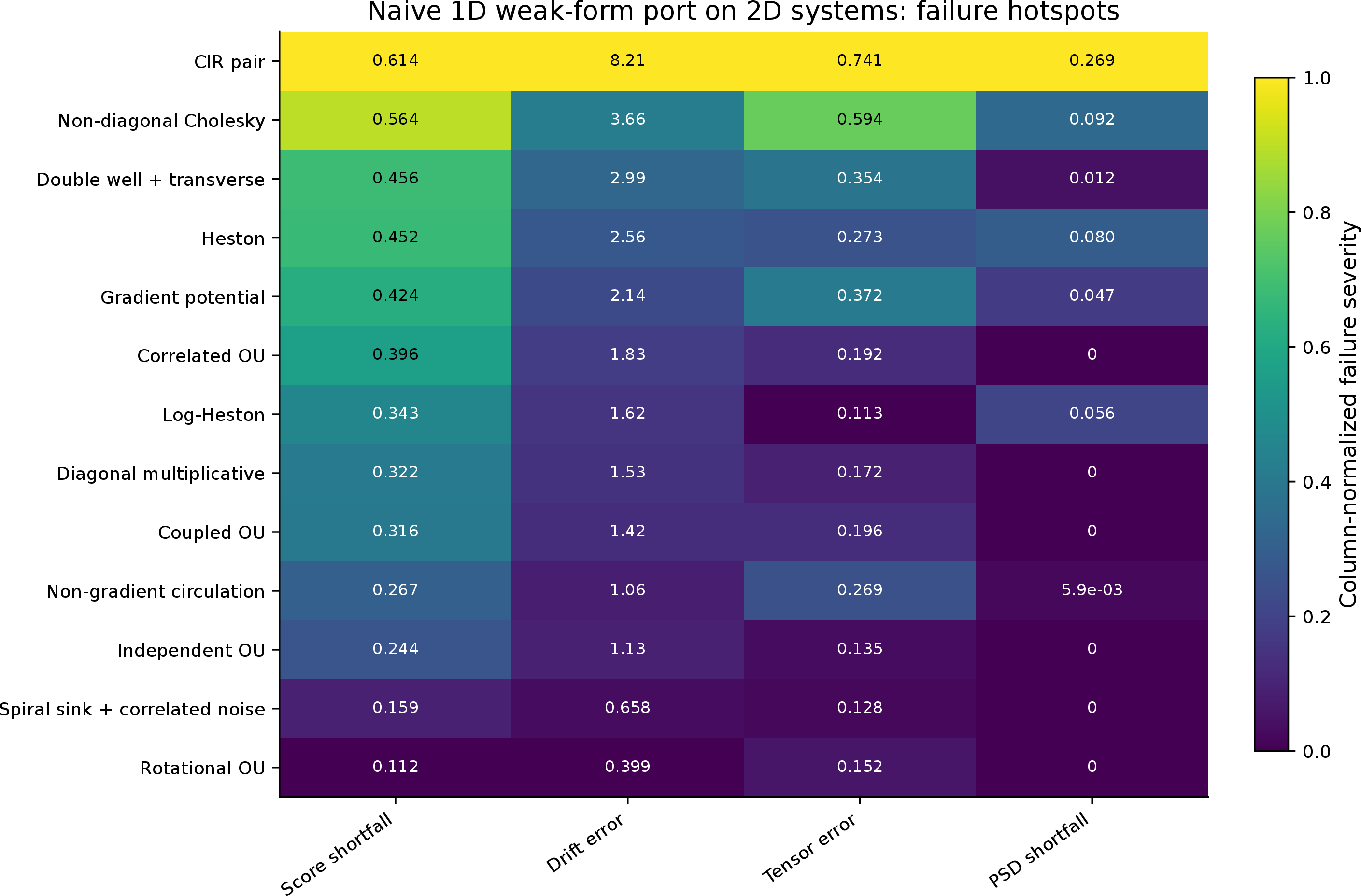
The natural first baseline is to run the one-dimensional estimator component by component on \(b_1\), \(b_2\), \(a_{11}\), \(a_{12}\), and \(a_{22}\). This keeps the adapted spatial-kernel identity but not the geometry needed in two dimensions: raw bivariate monomials are ill-conditioned on anisotropic state clouds, drift rows have unequal noise levels, and independently fitted tensor entries need not form covariance matrices. 1 shows that the dominant failure is drift in low-SNR or scale-disparate systems, with tensor and PSD failures appearing where the scalar fits ignore covariance structure.
4.3 Ablation: mechanism contributions↩︎
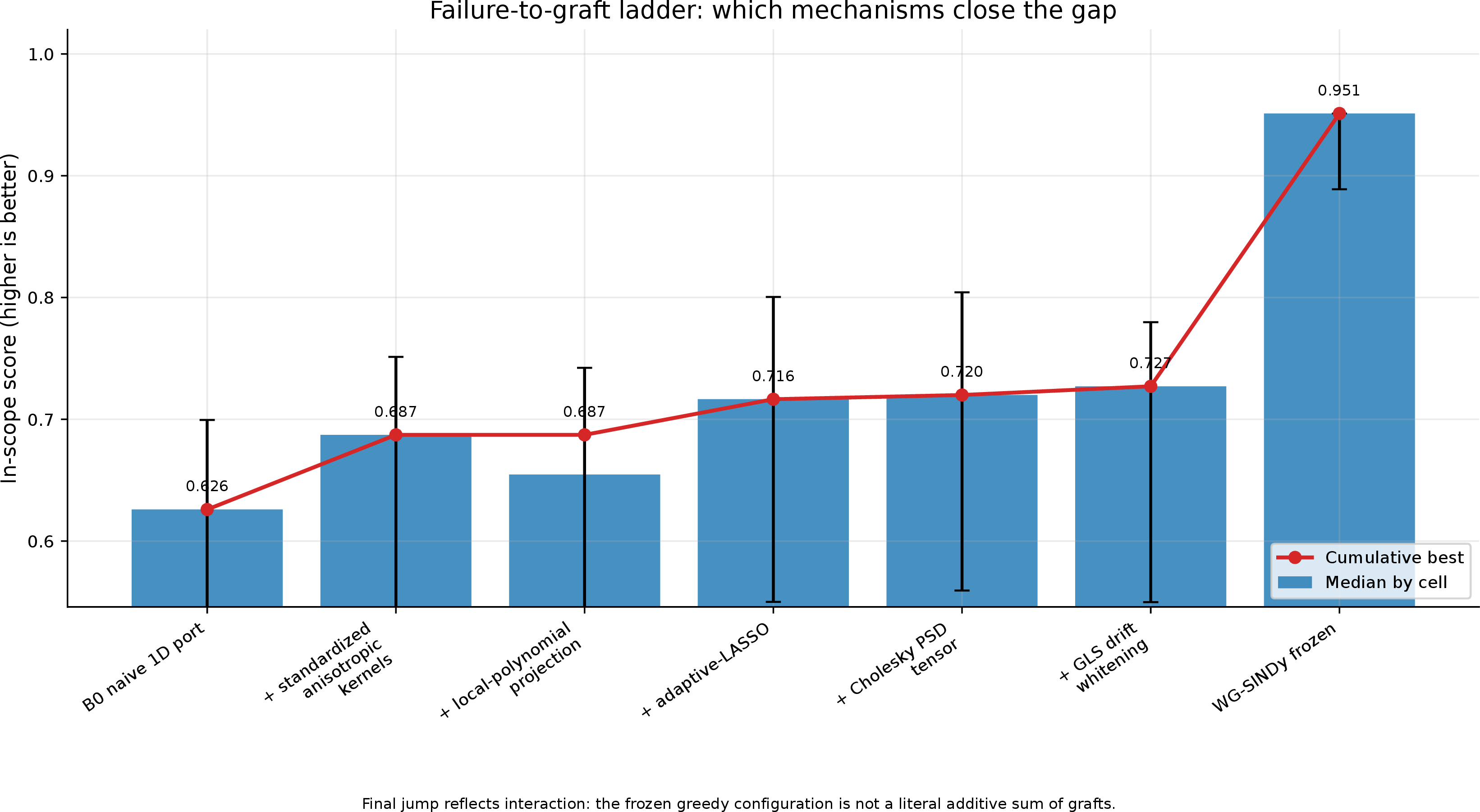
2 adds the mechanisms in the order used by the estimator: standardized anisotropic kernels, local-polynomial projection, adaptive sparsification, Cholesky tensor recovery, GLS drift whitening, and pooled trajectory selection. The score rises from the naive port to the frozen method, with the final jump reflecting interaction among jointly tuned components. 3 gives the leave-one-out view. Pooling, feasible GLS, and local-polynomial smoothing have clear in-scope effects in the checked-in necessity matrix. Cholesky recovery, adaptive LASSO, and anisotropic bandwidths are important structural or stress-regime safeguards, but this matrix does not by itself establish that each is empirically necessary on the in-scope median score.
4.4 Descriptive comparison with in-repository baseline proxies↩︎
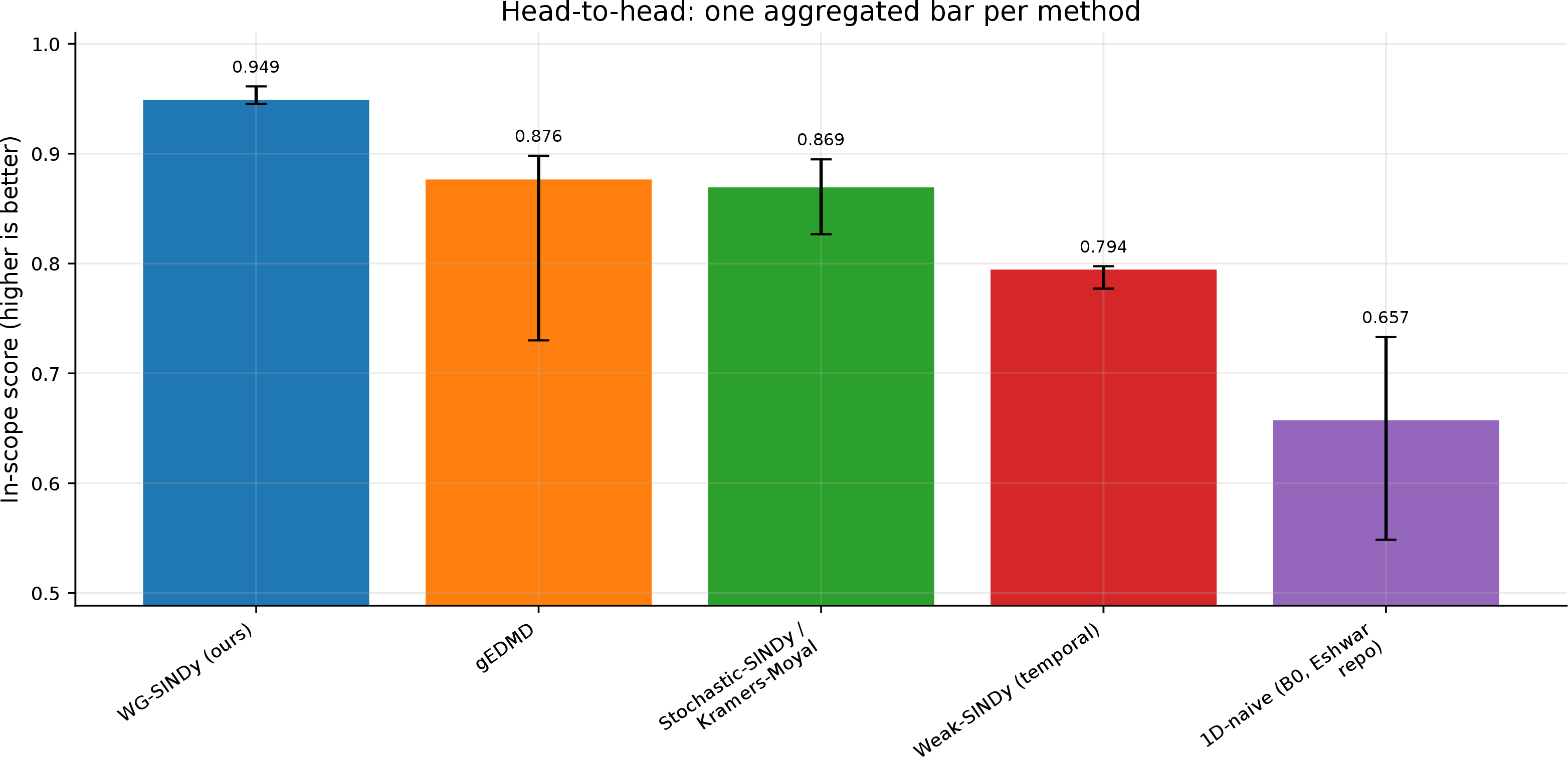
4 compares WG-SINDy with four lightweight in-repository baseline proxies: a local Kramers–Moyal/stochastic-SINDy moment estimator, a temporal Weak-SINDy proxy, a dense generator-EDMD proxy, and the naive one-dimensional weak-form port. These are method-family diagnostics rather than certified reproductions of the original published implementations. The data budgets are also unequal: WG-SINDy and the generator-EDMD proxy use \(R=16\), the local-moment and temporal-weak proxies use \(R=4\), and the naive port uses \(R=1\). The resulting scores are therefore descriptive and should not be interpreted as a controlled ranking of the underlying published methods.
4.5 Per-system baseline-proxy comparison↩︎
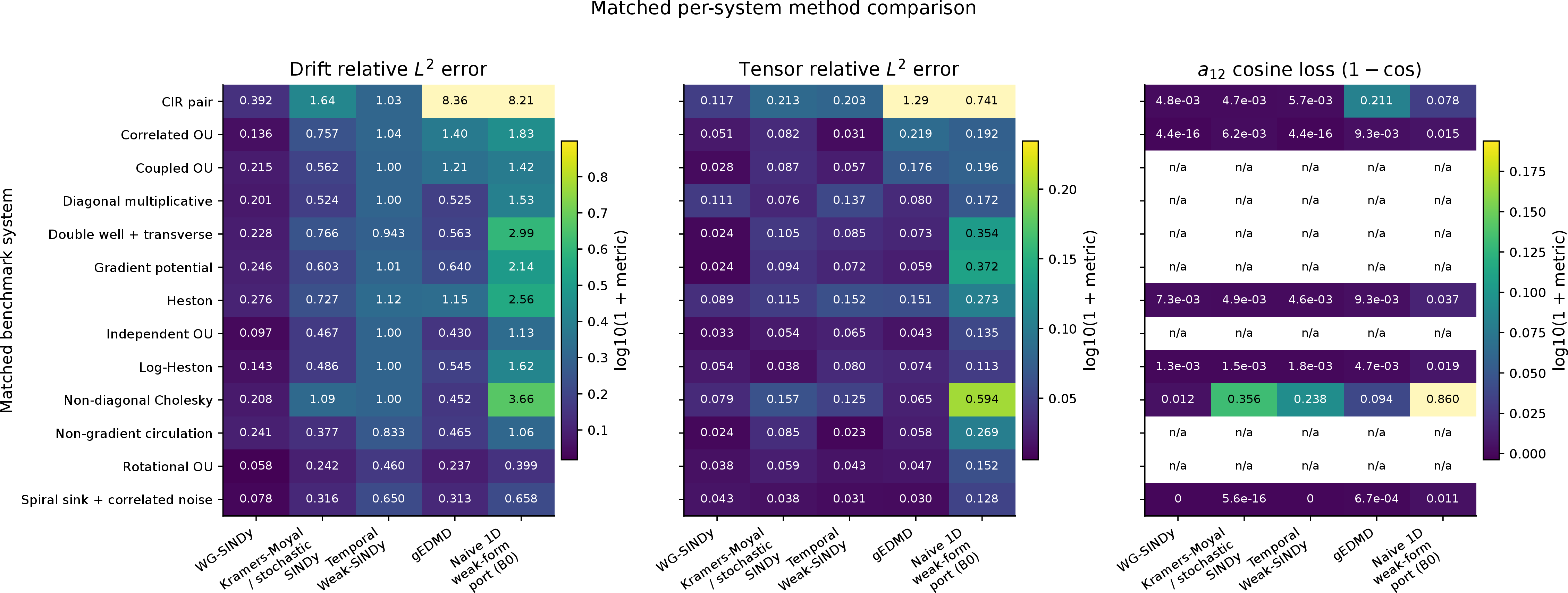
5 reports the same in-repository proxy comparison system by system. Cell values are the raw common metrics available from the shipped outputs. The colour transformation is used only for readability. Because these are proxy implementations with unequal trajectory budgets, the panel should be read as a failure-mode diagnostic rather than as evidence that one published method universally outperforms another.
4.6 The three read-outs↩︎
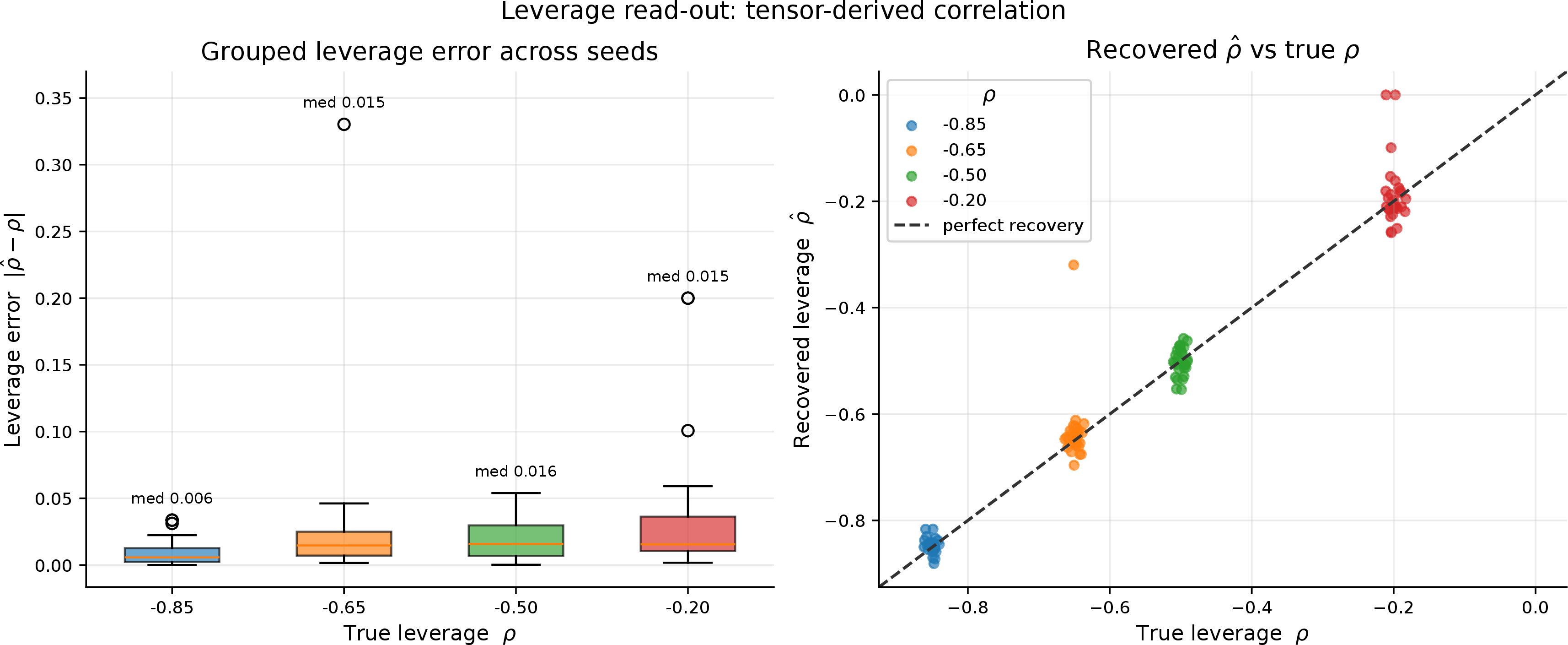
Once the generator is recovered, physical summaries become read-outs rather than separate fits. Normalizing \(\hat{a}_{12}\) by the diagonal tensor entries gives the instantaneous shock correlation, and 6 shows that its sign and magnitude are preserved across leverage regimes. The antisymmetric part of the recovered drift gives a drift-curl diagnostic; in the isotropic rotational OU case this diagnostic agrees with the stationary-current direction, while for nonlinear systems it is reported only as an antisymmetric-drift direction. The full tensor field provides the third read-out: local fluctuation geometry, shown in the datasheets.

4.7 Convergence and honest nulls↩︎
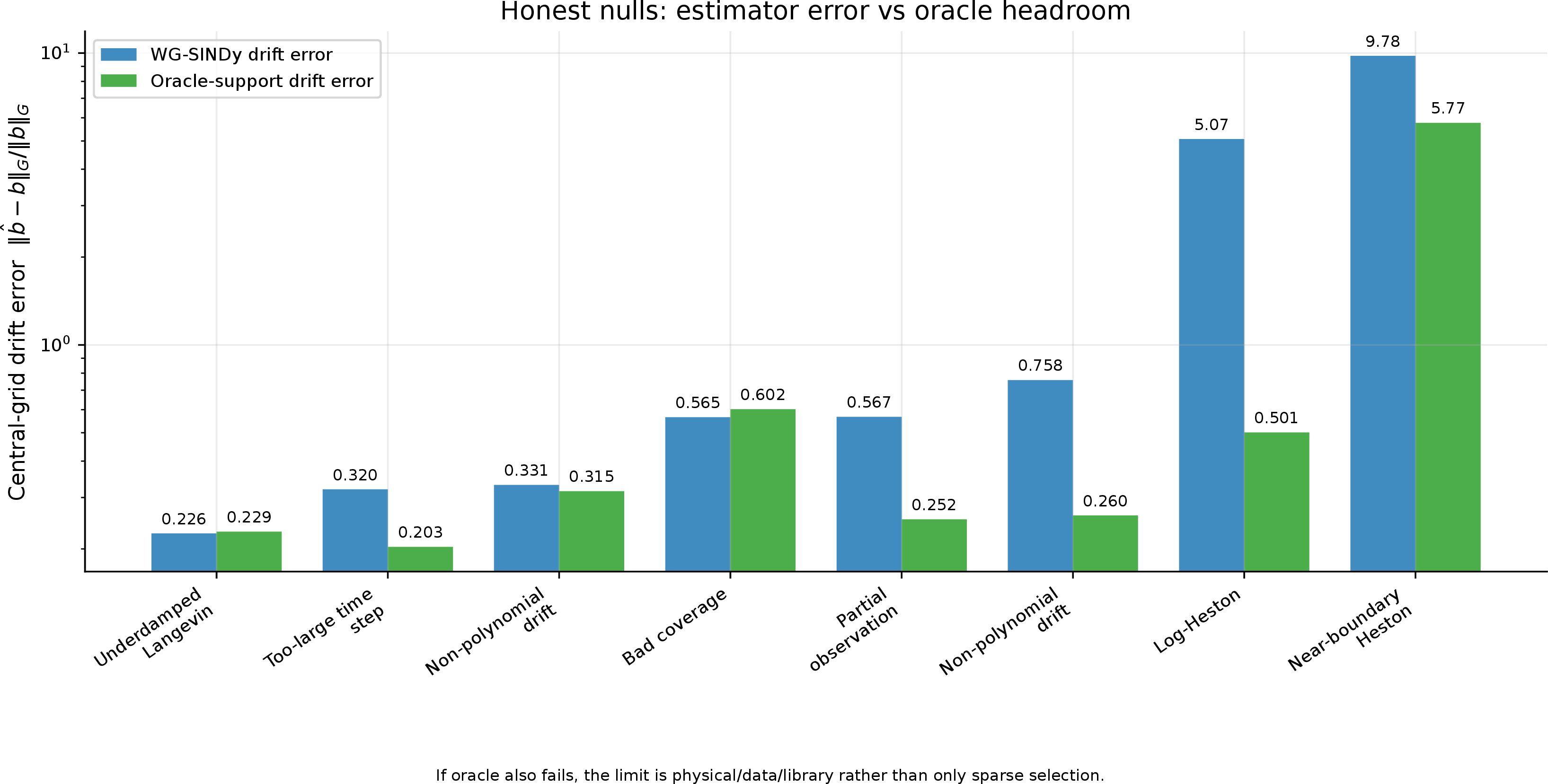
8 checks that errors decrease with effective horizon when the problem is identifiable, until finite-step, library, or conditioning floors dominate. 9 gives the complementary check by comparing WG-SINDy with an oracle-support solve on systems that violate recovery conditions. When the oracle also has large error, the failure is not sparse selection alone. The panel names the limiting axis—low drift SNR, near-singular tensors, boundary concentration, missing library terms, partial observation, insufficient coverage, or too-large \(\Delta t\)—so the method reports when the data do not identify the claimed symbolic generator.

5 Discussion and Limitations↩︎
5.0.0.1 How to read the relative errors.
The errors in 1 are generator-recovery diagnostics, not claims of sub-percent parametric precision. A useful recovery must select the right terms, suppress spurious ones, match the fields on the sampled region, recover the off-diagonal tensor direction when present, and return a valid covariance matrix. This is why field errors, support counts, off-diagonal cosines, and PSD fractions are reported separately.
The main limitation is the information content of the paths. The weak form removes derivative estimation and reduces martingale noise, but it cannot excite unvisited state regions, detect terms below the weak-row noise floor, or span a generator outside the library. Tensor and leverage terms in stochastic-volatility models are recoverable because they enter quadratic variation, while log-price drift is an \(O(\Delta t)\) signal hidden under \(O(\sqrt{\Delta t})\) fluctuations. Thus the method should be used with coverage, conditioning, support, and PSD diagnostics: when those checks fail, the sampling regime or library must change before a symbolic generator claim is defensible.
6 Conclusion↩︎
We extended weak-form spatial-kernel generator recovery from scalar diffusions to two-dimensional Itô systems. The extension is motivated by the adapted fixed-weight spatial identity used in the one-dimensional construction, while adding the machinery needed in two dimensions: standardized anisotropic kernels, local-polynomial weak projection, sparse adaptive selection, feasible GLS drift reweighting, a PSD Cholesky read-out, and trajectory pooling. Because the released smoother is estimated from the full sampled state cloud, the present paper treats this identity as population motivation rather than as an exact finite-sample unbiasedness theorem for the implemented estimator. The resulting frozen estimator recovers both drift components and the full symmetric diffusion tensor inside the declared identifiability envelope, including off-diagonal noise correlation, while returning a positive-semidefinite tensor by construction. The benchmark shows useful recovery across 19 in-scope systems and also identifies 10 systems where the data, library, or sampling regime do not support a stronger symbolic recovery claim.
Supplementary Material: per-system datasheets↩︎
The following per-system datasheets are supplementary. The main-text claims rest on the flagship examples (4.6) and the navigation index 1; each datasheet below gives the SDE, its analytic generator, the recovered symbolic coefficients, the recovered-vs-true fields, the quantitative verdict (with the failing axis named for limit cases, per 3.11), and a discussion. Systems are grouped by family.